
3
Processes That Cause Abrupt Climate Change
Weather changes abruptly from day to day, and there is no basic difficulty in understanding such changes because they involve a “fast” and easily observed part of the climate system (e.g., clouds and precipitation). But mechanisms behind abrupt climate change must surmount a fundamental hurdle in that they must alter the working of a “slow” (i.e., persistent) component of the climate system (e.g., ocean fluxes) but must do so rapidly. Two key components of the climate system are oceans and land ice. In addition, the atmospheric response is a crucial ingredient in the mix of mechanisms that might lead to abrupt climate change because the atmosphere knits together the behavior of the other components. The atmosphere potentially also gives rise to threshold behavior in the system, whereby gradual changes in forcing yield nearly discontinuous changes in response.
A mechanism that might lead to abrupt climate change would need to have the following characteristics:
-
A trigger or, alternatively, a chaotic perturbation, with either one causing a threshold crossing (something that initiates the event).
-
An amplifier and globalizer to intensify and spread the influence of small or local changes.
-
A source of persistence, allowing the altered climate state to last for up to centuries or millennia.
As discussed in Chapter 2, the Younger Dryas is the most studied example of an abrupt change and provides insights about possible mechanisms. In many ways the Younger Dryas serves as a defining event that embodies the notion of abrupt climate change. Heinrich and Dansgaard/Oeschger events are generally thought to be governed by physical laws that are closely related to those involved in the Younger Dryas; indeed, many consider the Younger Dryas to be just an unusually big Heinrich or Dansgaard/Oeschger event. However, there are potentially many types of abrupt change, as described in Chapter 2, so we need to consider the full array of possible processes, rather than only those currently in favor for explaining the Younger Dryas and Dansgaard/Oeschger events. Other major events of interest in the paleoclimatic records include decadal Holocene droughts, the dry-moist cycles of North Africa, the Little Ice Age, and the cooling event that occurred about 8,200 years ago (the “8.2K event”). Abrupt shifts in the dominant modes of the modern climate are also being documented, and the active mechanisms in these shifts might be relevant to larger abrupt changes in the distant past or in the future.
AN OVERVIEW OF MECHANISMS
Understanding and simulating abrupt climate change poses special challenges in climate science. Many climate changes are well described as relatively small deviations from a reference state, often assumed to be in equilibrium with external forcing. Powerful simplified conceptual approaches (“linearizations”) are therefore appropriate and can explain many features in a faithful way. In a linear model, doubling the forcing doubles the response. The linear approach does not hold for abrupt climate change, in which a small forcing can cause a small change or a huge one, so fully nonlinear and transient considerations and simulations are required. In particular, transitions between qualitatively different climate states, as are seen in the paleoclimatic records, require abandoning the “time-slice” perspective in which equilibrium runs of climate models under different forcings are used to try to infer the path of climate change.
Three past classical model types have been important in this context because of their ability to simulate paleo abrupt climate change either spontaneously or in response to changes in controlling parameters or external forcing. These are the two-box Stommel model (1961), simple energy-balance models such as that of Sellers (1969), and the Lorenz models (1963, 1990).
Using a two-box model of the thermohaline circulation (THC) of the ocean, Stommel (1961) showed that the different response times of the ocean surface to heat and freshwater perturbations give rise to multiple equilibria of the THC with very different characteristics. This implies that forcing and other conditions do not uniquely define the state of the climate system and that perturbations beyond thresholds can trigger transitions to other equilibrium states. The model presents some fundamental concepts and demonstrates the major sources of uncertainty in simulating abrupt climate change caused by a change in the THC. Multiple equilibria, however, would not occur if all processes were linear. The nonlinearity of the Stommel model arises because the flow field of ocean water transporting heat and salt is itself a function of temperature and salinity. Nonlinearities and multiple equilibria are the fundamental concepts behind the simulation of abrupt climate change.
Simple models of the energy balance of the atmosphere exhibit multiple equilibria. The model of Sellers (1969) is a typical case: a given amount of solar irradiation allows either a cold or a warm planet in equilibrium. The nonlinearity here is introduced by a special formulation of the snow-albedo feedback, which is operative only in a particular range of temperatures. A cold earth is snowy, and snow reflects sunlight and keeps the earth cold. A warmer earth has less snow, absorbs more sunlight, and so stays warmer. Abrupt change can be triggered by variations in total solar output or other parameters that influence the radiative balance, such as snow cover.
The Lorenz models (Lorenz, 1963, 1990) provide a highly simplified description of atmospheric circulation. In addition to multiple equilibria in particular ranges of parameters, these models exhibit self-sustained oscillations and chaotic behavior. A system oscillates near one of two preferred centers; abrupt change occurs when the system switches from one mean of oscillation to the other. In a Lorenz model, these transitions occur spontaneously.
These examples suggest that abrupt climate change can occur in (at least) three fundamentally different ways:
-
Abrupt climate change can be the response to a rapidly varying external parameter or forcing. If one views only the atmosphere-ocean system, massive sudden discharges of freshwater from disintegrating ice sheets on land would be an example of a sudden external influence. Nonlinearity
-
in the atmosphere-ocean system is not a prerequisite for such behavior, whose time scale is dictated essentially by that of the forcing.1
-
Slow changes in forcing can induce the crossing of a threshold and result in the transition to a second equilibrium of the system. The evolution of such a change would be governed by the system dynamics rather than by the external time scale of the slow change. In considering the whole earth system rather than just the oceans and atmosphere, massive discharges of freshwater from disintegrating ice sheets would be a result of threshold-crossing. Slow melting at the end of the last ice age produced ice-marginal lakes. When the ice margin reached a particular location, such as the path of a former river that the ice had dammed, a threshold was crossed, the ice dam broke, and the water was released rapidly (Broecker et al., 1988).
-
Regime transitions can occur spontaneously in a chaotic system. In this case, external triggers for transitions are not required, so a series of regime changes could continue indefinitely or until slow changes in external forcing or system dynamics removed the chaotic behavior.
Oceans
Changes in ocean circulation, and especially THC in the North Atlantic, have been implicated in abrupt climate change of the past, such as the Younger Dryas and the Dansgaard/Oeschger and Heinrich/Bond oscillations (Broecker et al., 1988; Alley and Clark, 1999; Stocker, 2000). Today, relatively warm waters reach high latitudes only in the North Atlantic. The high salinity of the Atlantic waters allows them to sink into the deep ocean when they cool, and warmer waters flowing along the surface then replace them. This yields a net heat transport into the high northern latitudes of the Atlantic and northward heat transport throughout the South Atlantic, carrying heat into the North Atlantic (Ganachaud and Wunsch, 2000; see also Plate 4b.)
Outburst floods, which would have freshened the North Atlantic and reduced the ability of its waters to sink, immediately preceded the coolings of the Younger Dryas and the short cold event about 8,200 years ago (Broecker et al., 1988; Barber et al., 1999); this suggests causation. Evidence of reduction or elimination of northern sinking of waters during cold times (Sarnthein et al., 1994; Boyle, 2000) provides further support, as does
the see-saw relation between Greenland and Antarctic temperatures on millennial scales (Blunier and Brook, 2001; see also Plate 2), which suggests that reduction in heat transport to the north allowed that heat to remain in the south.
Those and other considerations focus attention on changes in the THC as one cause of abrupt climate change. However, additional processes presumably were active in the past abrupt changes exemplified by the Younger Dryas, as indicated by the difficulty of fully explaining the paleoclimatic data on the basis of the single mechanism of North Atlantic THC changes. Therefore, the ocean’s role in climate is developed more fully in the following.
Water has enormous heat capacity—oceans typically store 10-100 times more heat than equivalent land surfaces over seasonal time scales, and the solar input to the ocean surface for a year would warm the upper kilometer only 1 degree—so the oceans exert a profound influence on climate through their ability to transport heat from one location to another and their ability to sequester heat away from the surface. The deep ocean is a worldwide repository of extremely cold water from the polar regions. If much of this water were brought to the surface in temperate or tropical regions, it could cause substantial cooling that, although transient, could last for centuries. It is not easy to bring cold water to the surface against a stable gradient, though, and this can happen only in special circumstances. Such localized change could, however, have a wider impact through atmospheric teleconnections. Fluctuations in ocean heat transport can also affect climate; for example, an increase in equator-to-pole heat transport would warm the polar regions (melting ice) and cool the tropics.
The implications of fluctuation in heat transport by the Atlantic THC have received particular attention, especially as a mediator of Younger Dryas and Dansgaard/Oeschger abrupt change. Deep water forms only in the North Atlantic and around the periphery of Antarctica, where extremely cold, dense waters occur. There is no deep-water formation in the North Pacific, because the salinity is too low to allow high enough density to drive deep convection, despite the low temperatures. By analogy, change in the freshwater balance of the North Atlantic, which might be caused by glacial discharge or warming of the planet through increases in carbon dioxide, potentially can act as a trigger to turn the THC on or off. In contrast, it is not thought that future climate change could turn on deep-water formation in the North Pacific, although there is evidence that at times during ice ages
the intermediate waters of the Northern Hemisphere Pacific were more ventilated than they are now (Behl and Kennett, 1996).
The threshold for deep-water formation cannot be thought of apart from the general circulation of the world ocean, because the density required for North Atlantic surface waters to sink is determined in relation to the “prevailing” deep-water density of the rest of the ocean. This density is determined globally and is intimately linked to processes in the Southern Ocean. Furthermore, the density of surface waters in the North Atlantic is not determined by purely local processes, in as much as the North Atlantic salinity is affected by mixing with transported subtropical Atlantic waters, whose salinity in turn is affected by tropical winds, which can systematically transport moisture out of the Atlantic basin. The freshwater balance of the Atlantic is further affected by melting of glaciers, transport of freshwater by sea ice, and land-surface processes that determine runoff patterns.
Several ocean heat-transport mechanisms other than the THC are in operation today. In particular, wind-driven ocean circulation dominates ocean heat transport in the North Pacific (Bryden et al., 1991) and the Indian Ocean (Lee and Marotzke, 1997). Results from relatively simple models suggest that in the absence of a vigorous THC, wind-driven heat and salt transports increase, making up at least in part for the loss of the THC as a transport agent (Marotzke, 1990; Winton and Sarachik, 1993).
Cryosphere
Land glaciers and sea ice enter into abrupt change mechanisms in many ways. The accumulation of ice on land and the associated ice-albedo feedback are probably too slow to be involved in abrupt climate change. However, because a glacier that is frozen to its substrate can surge if the basal temperature of the ice is raised to the melting point, glacial discharge and decomposition can be rapid (MacAyeal, 1993a,b; Alley and MacAyeal, 1994). Ice-sheet surging certainly would affect sea level, as noted in Chapter 4 with regard to the West Antarctic ice sheet. Surging also may affect the atmospheric flow pattern by changing the elevation of parts of the continental ice sheets (Roe and Lindzen, 2001). Furthermore, rapid glacial discharge can release armadas of icebergs into the ocean, which serve as an important indicator of abrupt climate change; increases in ice-rafted debris are the defining feature of Heinrich events (Broecker, 1994). More importantly, glacial discharge abruptly increases the delivery of freshwater to the ocean (to the North Atlantic, in the case of Heinrich events), with the po-
tential of modifying the THC. Another class of catastrophic event associated with land glaciers is the formation of large lakes of meltwater, held back only by fragile ice dams. The breaking of an ice dam can lead to the sudden delivery of massive amounts of freshwater to the ocean. As noted above, it is believed that the draining of an ice-dammed lake (Agassiz) was at least partly involved in the initiation of the Younger Dryas event and was most likely responsible for the event about 8,200 years ago (Barber et al., 1999; Broecker et al., 1988; Teller, 1990; Teller, in press).
Sea ice, which forms by freezing of ocean water, is an important amplifier of climate forcing. When sea ice forms, it increases the planetary albedo, enhancing cooling. Sea ice also insulates the atmosphere from the relatively warm ocean, allowing winter air temperatures to decline precipitously (as much as tens of degrees C, compared to conditions over open water), and reducing the supply of moisture to the atmosphere, which in turn reduces precipitation downwind. The rectifying and amplifying effects of sea ice are important in connection with changes in the location of North Atlantic deep-water formation. The site of North Atlantic deep-water formation is roughly where a substantial fraction of the heat transported northward in the Atlantic Ocean is deposited. Changes in the location affect the sea-ice margin and can have a net effect on the planetary radiation budget.
Formation of sea ice also leads to rejection of very dense brine. This is particularly important around the Antarctic margin. Brine formation there is the major contributor to formation of the world’s deepest ocean water.
Sea ice must be considered dynamically. Its movements are rather like those of a viscous fluid in coexistence with ocean water when viewed over a large enough area, but with brittle behavior in smaller regions. The creation of leads, or cracks, in sea ice affects albedo and air-sea exchange, and the movement of sea ice from one place to another has important effects on the global distribution of ice cover. Similar transport issues arise with regard to transport of icebergs discharged from land glaciers; here, the main interest concerns the distribution of freshwater ultimately delivered by the icebergs.
Snow cover can also serve as an amplifier of climate change and a source of persistence. Snow-covered land maintains cold conditions because of its high reflectivity and because its surface temperature cannot rise above freezing until the snow melts. There are interesting interactions between snow cover and vegetation. A modest snow cover on a flat surface, such as tundra, suffices to cause high albedo. However, in terrain covered with ever-
green trees, snow falls to the surface without completely coating the dark canopy, allowing absorption of much solar radiation.
Atmosphere
The atmosphere is involved in virtually every physical process of potential importance to abrupt climate change. The atmosphere provides a means of rapidly propagating the influence of any climate forcing from one part of the globe to another. Atmospheric temperature, humidity, cloudiness, and wind fields determine the energy fluxes into the top of the ocean, and the wind fields dictate both the wind-driven ocean circulation and the upwelling pattern (of particular interest in the tropics and around Antarctica). Atmospheric moisture transport helps govern the freshwater balance, which plays a crucial role in the THC, and precipitation patterns provide the hydrological driving of glacial dynamics. The atmospheric response to tropical seasurface temperature patterns closes the feedback loop that makes El Niño operate. Atmospheric dust transport can affect the planet’s radiation balance and on longer time scales might affect ocean carbon dioxide uptake via iron fertilization (Mahowald et al., 1999).
How do oceans affect the air-temperature pattern? The primary—although by no means the only—effect of oceans on air temperature derives simply from the heat capacity of the oceans and has little to do with horizontal ocean heat transport. Being composed of a fluid that can mix heat vertically, oceans are slow to cool in winter and slow to warm in summer. Land temperature, in contrast, responds rapidly to adjust to changes in the seasonal cycle of solar radiation. The primary winter pattern of surface air temperature thus consists of warm oceans and cold land (see Plate 5). To some extent, that contrast depends indirectly on ocean dynamics, which affect the upper ocean stratification and so the mixed-layer depth and the amount of seasonal heat storage (Plate 5).
Complete shutdown of the THC would remove about 8 W/m2 from the Northern Hemisphere extratropical heat budget (Pierrehumbert, 2000). To restore balance, the northern atmosphere-ocean system must cool down until the infrared radiation lost to space is correspondingly reduced. On the basis of a conventional sensitivity factor incorporating water-vapor feedback, the perturbation in heat budget implies an extratropical cooling of about 4°C, and growth of sea ice could amplify this cooling. This is roughly the cooling found in simulations (Seager et al., 2001), in which ocean heat transport was suppressed. Because the Northern Hemisphere THC is pri-
marily an Atlantic rather than Pacific phenomenon, the heat transport is focused in the Atlantic. The somewhat greater warmth of European coastal regions than of similar latitudes on the Alaskan coast might well be linked to this THC heat transport (Plate 5), although debate continues about where and by how much ocean heat transport warms the atmosphere, and the extent to which changes in oceanic heat transport would be balanced by changes in atmospheric heat transport.
Popular treatments sometimes imply that the THC is responsible not only for the temperature difference between Europe and Alaska, but also for the larger difference between Europe and the east coast of North America. This is unlikely because the US Pacific Northwest coast is warmer than the east coast of Asia without an active THC in the North Pacific. Two factors appear to provide the large differences between east and west coasts. First, the prevailing westerly winds pick up some heat during winter while blowing over the ocean, spreading the moderating influence of the ocean downwind. Second, and perhaps more important, the planetary wave pattern—the global-scale sinuous bending of the jet stream—brings Arctic air down over the US New England region and the Asian coast of the Pacific and warmer breezes to the US Pacific Northwest and Europe. The pattern is known to be driven primarily by mountains in the winter (Nigam et al., 1988), and is influenced relatively little by land-sea temperature contrasts. An improved quantitative understanding of the east-west (North America to Greenland to Europe) gradient of temperature fluctuations in past abrupt climate changes is crucial to furthering the understanding of mechanisms. On the other hand, the relative warmth of Norway, which is just to the east of the second major center of heat loss in the North Atlantic (the first being in the Gulf Stream off the coast of the United States), is probably due to the THC; the Pacific lacks similar warmth to that off Norway.
A major problem with THC-based theories of the Younger Dryas and Dansgaard/Oeschger events is that atmospheric models yield a predominantly local North Atlantic cooling in response to THC shutdown, with few of the global repercussions that seem to be demanded by the data (see Chapter 2). In fact, the atmosphere alone does not seem able to extend the influence of extratropical influences to the rest of the globe efficiently. Even such a major forcing as the introduction of Northern Hemisphere ice sheets of the last glacial maximum into models has little influence south of the equator (Manabe and Broccoli, 1985; Broccoli and Manabe, 1987). In models generally, North Atlantic cooling affects the strength of the tropical
Hadley circulation, which leads to some temperature change in the northern half of the tropics, and more important precipitation changes.
There have been a number of simulations of the atmospheric response to THC shutdown or to directly imposed North Atlantic sea-surface temperature perturbations. Fawcett et al. (1997) eliminated Nordic sea oceanic heat transport in the GENESIS model and found localized reductions in surface air temperature of as much as 24°C. Even with such an extreme cooling, the temperature perturbation is very localized. It amounts to only 2.8°C over the summit of Greenland versus about 8°C observed (Severinghaus et al., 1998) and 2°C or less over much of Europe, underestimating some changes based on proxy records. As summarized in Ágústsdóttir et al. (1999) and Fawcett et al. (1997), these experiments matched many aspects of changes reconstructed from proxy records (including changes in seasonality of precipitation in central Greenland and other such details) but generally underestimated the magnitude of reconstructed changes except close to the North Atlantic. It is difficult to determine how the oceanic heat transport involved in these experiments compares with the heat carried by the real THC.
Manabe and Stouffer (1988, 2000) carried out experiments with a coupled atmosphere-ocean model in which the THC was largely suppressed by a massive artificial injection of freshwater. They found a more moderate Atlantic surface cooling of 6°C with cooling of 1-4°C over Europe and the greatest coolings confined primarily to coastal areas. The atmospheric-response experiments of Hostetler et al. (1999), forced by imposed sea-surface temperature patterns, yield a quite different impression, as the North Atlantic cooling leads to temperature reductions in excess of 4°C over all of Europe and much of Asia. The general locality of atmospheric response in those simulations does not by any means disprove the THC theory of the Younger Dryas and Dansgaard/Oeschger events. Current atmospheric models might be missing some crucial physical feedbacks that allow the real atmosphere to exhibit such large and widespread responses to THC changes. This is an unsettling possibility, in that it suggests that models could also fail to anticipate the threat of surprising and abrupt changes, which might occur in connection with global warming, as indicated in Plate 7 and discussed extensively in Chapter 4.
Ocean dynamics could help to extend northern extratropical influences to the tropics and to the Southern Hemisphere, and indeed ocean circulation experiments show some global changes in response to North Atlantic freshwater pulses. A full treatment of the role of the oceans must be carried
out with coupled atmosphere-ocean models. There have not yet been any successful simulations of the pattern and magnitude of the Younger Dryas or of recurrent Dansgaard/Oeschger events with coupled ocean-atmosphere general circulation models. And there have not been any integrations of coupled ocean-atmosphere models over sufficiently long time scales to determine the natural level of millennial variability in such models, particularly in glacial conditions. Despite considerable success in modeling some aspects of past abrupt climate changes, there is much work still to be done.
Fluctuations in the atmospheric carbon dioxide concentration (Petit et al., 1999) have played a crucial role in climate change on the glacial-inter-glacial time scale (Pollard and Thompson, 1997). According to general circulation model results (Manabe and Broccoli, 1985), without the reduced greenhouse effect arising from low carbon dioxide in glacial times, the Southern Hemisphere would have experienced little cooling despite the massive growth of Northern Hemisphere ice sheets. However, carbon dioxide fluctuations are not radiatively significant on the time scale of the Younger Dryas or Dansgaard/Oeschger events, and up to industrial times carbon dioxide had only insignificant fluctuations throughout the Holocene. Methane is an important greenhouse gas and did fluctuate markedly in the course of many abrupt-change events, with changes in low-latitude and high-latitude sources (Brook et al., 1999). The low-latitude source changes are generally thought to be indicative of changes in tropical hydrology, so methane serves as an important indicator of the involvement of the tropics in abrupt climate change (Chappellaz et al., 1997). However, the magnitudes of methane changes were too small to yield appreciable radiative forcings, and the observation that temperature changes in Greenland preceded methane changes (Severinghaus et al., 1998) is not generally consonant with driving by a methane greenhouse effect.
Water vapor is an important greenhouse gas, but it is different from carbon dioxide and methane in that its concentration is determined primarily by atmospheric temperature and circulation patterns rather than by sources and sinks (Held and Soden, 2000; Pierrehumbert, 1999). Most of the atmosphere is highly undersaturated in water vapor and thus could hold considerably more than it does at present. The undersaturation is particularly prominent in the tropics, so reorganizations of the atmospheric water-vapor distribution stand as a possibility for amplifying and globalizing abrupt climate change. There are intriguing possibilities for interaction between water-vapor feedback and dust fluctuations, inasmuch as dust and other aerosols can serve as cloud condensation nuclei (Durkee et al., 2000).
By affecting precipitation efficiency, that process can potentially alter the water vapor content of the atmosphere. In addition, dust that absorbs solar radiation can affect precipitation through the circulation that arises in response to such heating.
Mechanisms centered in the tropics, particularly the tropical Pacific, have received increasing attention in recent years. The tropics have a compelling advantage over the North Atlantic as a mediator of global climate change. Because of the relatively weak confining influence of the earth’s rotation at low latitudes, the effect of local changes in sea-surface temperature is communicated almost instantly through the atmosphere to the entire tropical band. This confining influence is due to the earth’s rotation, which causes the well-known Coriolis effect in which all atmospheric and oceanic flows turn relative to the surface beneath them (to the right in the Northern Hemisphere and to the left in the Southern Hemisphere) rather than proceeding directly from regions of high to low pressure. The degree of turning is proportional to the sine of the latitude, so turning disappears at the equator. The strong high-latitude tendency for wind and ocean currents to turn slows the transmission of information through the climate system, whereas the weaker turning tendency near the equator allows rapid communication.
Tropical forcings create circulation patterns that have a major remote impact in the middle-latitude and polar regions, again communicated through the atmosphere. The tropical atmosphere-ocean system offers a rich palette of possible amplifiers and switches that could in principle lead to abrupt climate change. The dominant atmospheric circulation in the tropics is an overturning motion known as the Hadley cell, with air rising in warmer regions near the equator, spreading at high altitude, sinking in the subtropics, and returning along the surface. This circulation has a profound effect on tropical water vapor, cloudiness, and convection, with rain forests under the rising limb and deserts under the descending air. The Coriolis turning of the return flow along the surface yields the surface easterlies that drive the ocean. The upper branch of the circulation affects middle-latitudes through its influence on the upper-level subtropical jet.
Shifts in the position of the rising branch (the intertropical convergence zone, or ITCZ) can lead to major changes in the strength of the circulation (Hou and Lindzen, 1992; Lindzen and Hou, 1988), and it has been suggested that ITCZ shifts could amplify abrupt climate change (Clement et al., 2000). Model results suggest that changes in North Atlantic temperature associated with cutoff of the THC cause substantial changes in the Hadley circulation, propagating the influence of THC shutdown into the
tropics (Manabe and Stouffer, 1988; Fawcett et al., 1997) and causing changes in tropical precipitation. In simulations, imposed North Atlantic cooling causes enhanced wind-driven oceanic upwelling in tropical and extratropical regions, which would bring colder waters to the surface and thus might contribute to additional cooling (Ágústsdóttir et al., 1999). There are many possibilities for regime switches lurking in the collective behavior resulting from coupling the Hadley cell to ocean dynamics.
El Niño is an oscillation of the coupled tropical atmosphere-ocean system. The influence of El Niño extends strongly into the extratropics. How much would El Niño change in a warmer or colder climate? Interest in that question has sharpened because there are indications that the character of El Niño events underwent a shift beginning in the 1970s. Carbon-14 data from corals suggest that changes in upwelling and in the source of subsurface water were involved in the shift (Guilderson and Schrag, 1998). Furthermore, comparisons with prehistoric El Niño records recovered from corals from the Last Glacial Maximum and from the previous major interglacial suggest a systematic relation between global conditions and the temporal character and amplitude of El Niño (Hughen et al., 1999; Tudhope et al., 2001).
Changes in El Niño are important in themselves because El Niño is by far the largest interannual climate signal at present and in the past, but it is possible that such changes might also mediate widespread changes in the global climate regime. Tropical transient motions, including those associated with El Niño, affect the water vapor and cloud distribution and hence the global energy budget (Pierrehumbert and Roca, 1998; Pierrehumbert, 1999). Tropical sea-surface temperature fluctuations, in contrast with those in the middle latitudes, cause variations in deep atmospheric heating, in turn giving rise to waves that powerfully communicate their influence to the rest of the planet. Any change in one part of the tropics tends to drag along the temperature of the entire tropical free troposphere owing to the tight coupling enforced by the Hadley and Walker circulations. The tropics are thus a natural candidate to be a “globalizer” of climate influences. The El Niño cycle might also affect transport of freshwater between the Atlantic and Pacific basins through its influence on low-level wind patterns (Latif et al., 2000; Schmittner et al., 2000). In addition, wind shifts affect the patterns of tropical upwelling and subtropical ocean gyres, possibly leading to changes in heat transport out of the tropical oceans. A treatment of some of the factors governing heat transport within the tropics and subtropics
can be found in Lu et al., (1998), Lu and McCreary (1995), and McCreary and Lu (1994).
Low clouds have an albedo that is not very different from that of sea ice, but they can form almost instantaneously and are very sensitive to the structure of the tropical boundary layer. Increase in low cloud cover has a cooling effect, whereas dissipation of low clouds has a warming effect. The occurrence of low clouds is not solely, or even primarily, a function of temperature. Cloud properties are influenced by dust and aerosols, and an increase in these can make it easier for water to condense into small droplets, yielding brighter clouds and affecting precipitation. All these effects are subject to considerable uncertainties, and they remain as possibilities for mediating abrupt climate change or amplifying effects of THC fluctuations.
Land Surface
Land-surface processes can participate in abrupt climate change in many ways. The albedo of the land surface can change greatly, with fresh snow or ice sheets reflecting more than 90 percent of the sunlight striking them but dense forests absorbing more than 90 percent. Changes in surface type thus can affect solar heating and feed back strongly on climate. Rainfall used by plants and transpired to the atmosphere contributes substantially to local cooling during evaporation, and it supplies clouds and additional rainfall. Rainfall not used by plants typically runs off in rivers to the ocean, freshening surface waters at outflows but leaving low humidity in air over land. Thus, changes in vegetation have effects well beyond localities where the changes occur.
The land surface is the major source of dust, smoke and soot, and a variety of biogenic emissions. These affect cloud formation and albedo, drop size and rainout, and clear-sky radiation. Again, changes in the land surface can feed back on climate. The roles of these and other land-surface processes in causing, amplifying, or allowing the persistence of abrupt climate change are at best poorly understood. Additional work, especially in land hydrology and dust-cloud processes, is warranted.
External Forcings
A few types of forcings external to the climate system could play roles as pacemakers of abrupt climate change. These forcings vary too slowly to be prime movers of abrupt change, but if the climate system exhibits discontinuous response to continuous variations of some forcing parameters,
then the possibility exists that external forcing variations might determine the timing of events.
For example, the earth’s orbital parameters vary over time, affecting the distribution of solar energy delivered to the planet in time and location. The fastest of these variations is the precessional cycle, which takes about 22,000 years to complete and determines when the summer solstice occurs relative to the time of closest approach of the earth to the sun. In the tropics, that yields an 11,000 year half-precessional rhythm, and there are substantial changes in the insolation pattern over as little as 5,000 years. Those changes could have a major impact in the tropics through their effect on the latitudinal excursion of the ITCZ and its consequent effects on the Hadley circulation. The effect of precessional insolation changes on monsoonal circulations has been implicated in the moistening and drying of the Sahara, with strong feedbacks linked to land-surface processes, including changes in vegetation (Kutzbach et al., 1996; Claussen et al., 1999; Carrington et al., 2001). Precessional insolation changes possibly could have large effects on El Niño occurrence (Clement et al., 2000, 2001).
The effects and magnitude of fluctuations in solar output are less well constrained. There is an observable modulation of the sun’s brightness over the 11-year solar cycle, but this is too frequent an effect to alter climate much. On longer time scales, there are no direct observations of the fluctuation of solar output. Observations and proxies for solar activity going back centuries or more do indicate long-term fluctuations in activity, as measured by sunspot number or solar-wind effects; it is not known how much fluctuation in solar brightness goes with such fluctuations in activity. It has been suggested that the solar influence on climate can be mediated directly by the influence of cosmic-ray fluxes (modulated by the solar wind’s effect on the earth’s magnetic field) on cloud formation (Svensmark and FriisChristensen, 1997; Svensmark, 1998), but the magnitude or even sign of the effect has not yet been quantified. Solar influences have been suggested as the cause of the Little Ice Age (Broecker, 1999), and indeed changes in solar activity do seem to line up with some major climate fluctuations. Solar forcing has been tied to drought frequency and effects on Mayan civilization (Hodell et al., 2001).
Exotica and Surprises
In addition to the well-studied mechanisms detailed above, there might be other threshold phenomena in the climate system that are difficult to assess quantitatively. The possibility of catastrophic release of methane by
breakdown of frozen gas-ice compounds (clathrates) in permafrost or the ocean floor is in this category. Methane release has been clearly implicated in the warm event at the end of the Paleocene (Kennett and Stott, 1991; Dickens et al., 1995) (Box 4.1), and it has been argued that some of the Pleistocene methane signal is due to clathrate decomposition (Kennett et al., 2000) rather than tropical or high-latitude hydrological circumstances.
Furthermore, it must be acknowledged that the earth’s climate system has in the more distant past exhibited major switches in mode of operation that are simply not understood. Notably, the past climate has oscillated between hothouse climates lasting tens of millions of years, when there was little or no permanent polar ice, and icehouse climates like those of the present and the Pleistocene. Both states have occurred throughout geological history. The most recent period of increased warmth continued throughout the Cretaceous (65 million years ago) into the Eocene (55 million years ago) and terminated with the onset of major ice ages about 2 million years ago. However, there were also icehouse periods earlier in the earth’s history, including times during the Carboniferous and the Neo-Proterozoic. Although it is generally believed that geochemically mediated changes in atmospheric carbon dioxide played a major role in such transitions, there has been little success in reproducing the key features of hothouse climates by increased carbon dioxide alone. Concentrations of carbon dioxide high enough to prevent permanent polar ice in models generally lead to simulation of tropical oceans warmer than suggested by available data (Manabe and Bryan, 1985); the realism of both the tropical temperatures and the very high carbon dioxide levels are still under debate (Pearson et al., 2001). It had been hoped that better understanding of dynamic ocean heat transport would solve the problem, but recent work on Cretaceous and Eocene ocean dynamics does not support this idea. Moreover, even in simulations with increased carbon dioxide, continental interiors become too cold in the winters to reconcile with the equable climate that the fossil record demands. The problem of hothouse-icehouse transitions underscores that as-yet-unidentified mechanisms for mediating radical changes, some of which could well be abrupt, are lurking in the climate system.
Compounding the mystery of initiation and maintenance of the above “hot” mode of the climate is the growing evidence that the earth has fallen into an extremely cold “snowball-earth” state, in which the entire planet became ice-covered. The most recent occurrence of a snowball state was in the Neo-Proterozoic, about 600 million years ago. The circumstances in which the Snowball can be triggered are hotly debated but almost certainly
involve reduced solar intensity, low carbon dioxide, ocean heat transport, and dynamics of sea ice (Hoffman et al., 1998; Poulsen et al., 2001; Hyde et al., 2000).
ABRUPT CLIMATE CHANGE AND THERMOHALINE CIRCULATION
The previous section explored a variety of mechanisms that might be involved in abrupt climate change. However, because sudden change in the THC stands as the only well-developed theory to explain abrupt climate changes, such as the Younger Dryas and the Dansgaard/Oeschger and Heinrich events, we now investigate this phenomenon in greater detail. This is not intended to imply that other mechanisms in this rapidly evolving field will not be found that could also contribute substantially to abrupt climate change, but only that models for other such mechanisms are not as mature as for THC changes.
Processes Driving the Thermohaline Circulation
The global THC consists of: cooling-induced deep convection, brine rejection, and sinking at high latitudes; upwelling at lower latitudes; and the horizontal currents feeding the vertical flows. Contrary to widespread perception, convection and sinking are neither the same nor co-located (Marotzke and Stott, 1999) because when rotational effects are strong, flow tends to be around a patch of maximal surface density (characterizing convection) rather than into it (Marshall and Schott, 1999). In the North Atlantic, where much of the deep sinking occurs (Gordon, 1986; Ganachaud and Wunsch, 2000), the THC is responsible for the unusually strong northward heat transport; part of this heat is imported from the Southern Hemisphere. Much of this heat is given off to the atmosphere over the Gulf Stream, from where it is transported northeastward by the atmosphere. This part of the heat loss is typical of all subtropical gyres and is not associated with the global overturn (Talley, 1999). The enhanced heat transport has been believed by many to contribute to the relative mildness of western European climate, particularly that of Scandinavia. However, as described earlier in this chapter, the relative contributions to European climate of the THC, the wind-driven ocean circulation, atmospheric transport associated with land/ocean contrasts, atmospheric planetary waves, and so on, remain uncertain.
The THC is maintained by density contrasts in the ocean, which themselves are created by atmospheric forcing (air-sea heat and water fluxes) and modified by the surface circulation. A crucial question is which density contrast one should consider—the one between the equator and the poles, or the one between North and South Atlantic, or perhaps even between North Atlantic and North Pacific. The choice matters in assessing what order of magnitude of change in surface density it might take to change the THC drastically. “Pole-to-pole” density differences are about 1 order of magnitude smaller than “pole-to-equator” ones and hence much more easily influenced.
Surface-density contrasts can be influenced by a wide variety of processes, both internal to the ocean and coupled to the atmosphere. For example, the THC transports relatively warm and salty waters from the subtropical North Atlantic into the convection regions, with opposite effects on density. The import of warm water tends to reduce the density in the high latitudes, and the import of saline water increases density. An indirect effect is associated with evaporation (and later export of water vapor), which occurs preferentially over warm water. Analysis of atmospheric data suggests that the Atlantic drainage basin loses moisture to the Pacific (Warren, 1983; Zaucker and Broecker, 1992). The resulting accumulation of salinity in the Atlantic is compensated for by a net influx of freshwater from the Southern Ocean to the Atlantic. Changes in the water balance of the tropics (for example, changing El Niño patterns) might influence the THC if sustained long enough (Schmittner et al., 2000; Latif et al., 2000). Another important driver is sea ice (Aagard and Carmack, 1989), which is important for the freshwater budget of the North Atlantic convection regions. Thus, the central question in understanding and simulating the role of THC changes in abrupt climate change is: What is the combined effect of all these feedback mechanisms in a climate-change scenario?
An understanding of abrupt climate change thus requires a detailed quantitative knowledge about the various driving processes and their combined effect on the THC. In principle, a change in any of these processes can generate substantial climate change in areas influenced by the THC. However, those climate changes will not necessarily be limited to those areas. Effects could be widespread, and vary from region to region, because of changes in patterns of natural climate variability (such as NAO and ENSO) and their associated teleconnections. This is largely unexplored terrain that needs enhanced research.
A Model Hierarchy to Investigate Abrupt Climate Change
Research by Bryan (1986) marked the beginning of realistic process modeling of the THC. This work showed that the THC in a three-dimensional ocean model can assume multiple equilibria with vastly different locations of deep-water formation. Marotzke and Willebrand (1991) found four qualitatively different equilibrium solutions in an idealized global model of the THC. Common to these models was a special formulation of the surface boundary conditions that took into account the different response characteristics of the sea surface to changes in atmosphere-ocean heat and freshwater fluxes. Multiple equilibrium solutions were reported also in a fully coupled atmosphere-ocean model (Manabe and Stouffer, 1988); thus, the result does not depend on the specific simplifications used in the ocean-only models.
Slow changes of the surface freshwater balance constitute one possible mechanism to induce abrupt change. Using an ocean-only model, Mikolajewicz and Maier-Reimer (1994) demonstrated that switches in the THC occurred if the discharge of freshwater to the Atlantic exceeded a threshold value. Other coupled models used freshwater pulses to disturb the circulation and exhibit responses that range from a large reduction (Manabe and Stouffer, 1997) to a full shutdown of the THC (Mikolajewicz et al., 1997; Schiller et al., 1997).
These models suggest that the large changes observed in the paleoclimatic records were due to rapid changes in the THC. A more systematic investigation, however, was difficult to perform with the models because of their high computational burden. Extensive parameter studies, the basis of the advancement of understanding, are hardly possible. In recent years, simplified climate models—or climate models of reduced complexity—have been developed (Stocker and Marchal, 2001). They contain limited dynamics and have high computational efficiency. This was a crucial step forward in extending the toolbox to investigate abrupt climate change. Such models are also referred to as “earth-system models of intermediate complexity.” There are three strategies for formulating such models:
-
Rigorous reduction of the governing equations of the climate system.
-
Combination of model components of differing complexity.
-
Mathematical linearization of the response of comprehensive climate models to pulse perturbations.
Only strategies 1 and 2 are applicable to the problem of abrupt climate change, because of the nonlinear nature of the phenomenon. Coupled climate models of reduced complexity have been obtained with either strategy. Following the first, by zonally averaging the equations of motion in the ocean (e.g., Marotzke et al., 1988; Wright and Stocker, 1991), a very efficient ocean model component is obtained, which can be coupled to an energy balance model of the atmosphere (Stocker et al., 1992) or a statistical-dynamical model of the atmosphere (Petoukhov et al., 2000). The choice implies that the focus of investigation is restricted to the latitude-depth structure of the flow and to a priori chosen time scales that are accessible with these models. The second strategy was followed when three-dimensional ocean-circulation models were combined with a latitude-longitude energy balance model (Fanning and Weaver, 1997) or with an atmospheric-circulation model of reduced complexity (Opsteegh et al., 1998). Such combinations can be integrated for many thousands of years, thanks to the relative simplicity of the atmosphere.
Overall, models of reduced complexity are highly useful tools in paleoclimate research, and in particular for investigations of abrupt climate change, provided that they are used wisely. Clearly, they cannot replace general circulation models (GCM), because the reduced-complexity models consider only a limited set of constraints that are important in the climate system. The weaknesses of the reduced-complexity models are the incompleteness of dynamics and their often reduced resolution. Their strength is their computational efficiency, which permits extensive sensitivity studies or ensemble or even Monte Carlo simulations. Single simulations with reduced-complexity models are not useful to advance the science even if they happen to agree well with paleoclimatic data. However, these models are key tools in the process of quantitative hypothesis-building and -testing, not only in paleoclimatology but also in climate dynamics in general, because they allow the investigation of some feedback or process in its purest, isolated form. Often, the understanding gained from the reduced model is used to interpret the results from complex models. In addition, results from simple models or conceptual considerations have helped to define the strategy pursued in the use of complex models. In the following section, the committee adopts this approach to investigate the most fundamental questions concerning the stability of the THC and its role in abrupt climate change.
Abrupt Change, Thresholds, and Hysteresis
According to the definition given in Chapter 1, a climatic response faster than a change in forcing would be called abrupt. Such a rapid response would not occur as a result of small perturbations about a reference state, but only if a threshold was crossed; after that, a new state would be rapidly approached. Systems that exhibit such behavior often show hysteresis; that is, even if the perturbation has ceased after leading to the crossing of a threshold, the system does not return to its original state. Box 1.1 showed a
|
Box 3.1 Thresholds and Hysteresis 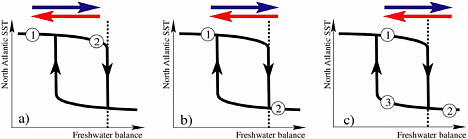 FIGURE 3.1 Many simple physical systems exhibit abrupt change, as demonstrated in the simple diagram presented in Box 1.1. The more complex figure (Figure 3.1 ) provides a schematic view of hysteresis in the thermohaline circulation. The upper branch denotes climate states in which the THC is strong and North Atlantic temperatures are relatively high (similar to present conditions). The lower branch represents a much-reduced or collapsed THC, in which the Atlantic meridional heat flux by the ocean is small. A given perturbation (indicated by the horizontal arrows) in the freshwater balance of the North Atlantic (precipitation plus runoff minus evaporation) first causes transitions from an initial state 1 to state 2. The reverse perturbation then causes a transition back to state 1, or to state 3. Three structurally different responses are possible for the same pair of perturbations, depending on whether threshold values (dashed line) are crossed. This, in turn, depends on where state 1 is, relative to the threshold: a) small, reversible response; b) large, reversible response; c) large, irreversible response (Stocker and Marchal, 2000). |
mechanical analogue of such behavior; Box 3.1 presents a sketch of hysteresis of the THC resulting from perturbations in the freshwater forcing.
The simplest variant of a hysteresis loop is a useful tool to discuss the different possibilities for how the climate system can respond to changes in some controlling variable. More freshwater increases the buoyancy of the surface waters and tends to reduce the strength of the THC; less freshwater makes the THC more stable. This is illustrated by the change in the location of the system on the upper branch of the hysteresis. As long as perturbations do not exceed thresholds, the system response is weak (Figure 3.1a). An abrupt change is triggered on the crossing of a threshold. A small change in forcing can then cause large additional perturbations (Figure 3.1b). If the initial state of the ocean-atmosphere system is a unique equilibrium, the system jumps back to the original state once the perturbation has ceased; the abrupt change is reversible. However, if other equilibria exist, the perturbation can cause an irreversible change (Figure 3.1c), unless a perturbation is applied that has the opposite sense of the original one and is large enough; in Figure 3.1c, state 3 would have to be pushed to the left, beyond the upward-pointing branch.
Experiments with simplified ocean-circulation and climate models have helped to discover the possible hysteresis behavior of the atmosphere-ocean system. As shown in Box 3.1, hysteresis is one manifestation of multiple equilibria in a nonlinear system. The existence of hysteresis for the THC was first shown by Stocker and Wright (1991), who used a simplified model. For some values of the freshwater balance of the North Atlantic, the THC can be either in a strong or in a collapsed state. Numerous studies with a variety of ocean models coupled to simple representations of the atmosphere have demonstrated the existence of hysteresis (e.g., Mikolajewicz and Maier-Reimer, 1994; Rahmstorf and Willebrand, 1995); this is a robust property of such models. Obviously, in more-complex models, the hysteresis can consist of a number of sub-branches nested in a complicated way. However, it is unclear whether the hysteresis behavior would persist in more-realistic coupled models, particularly if the ocean component has spatial resolution believed to be necessary to be quantitatively consistent with observations. Likewise, it is unclear where the climate system is now on the hysteresis curve of the Atlantic THC: What is its structure? Does it have thresholds? If so, how close is the threshold? The following discussion demonstrates how model- and parameter-dependent the answer can be.
Abrupt Climate Change in a Minimal Model of the Thermohaline Circulation
The response of the THC to a perturbation of the surface freshwater balance can be illustrated in the two-box model of Stommel (1961), which is explained in Box 3.2. A new addition to the original system is horizontal diffusion. It reflects the transport of salinity by the ocean gyres, the midlatitude systems of ocean circulation characterized by swift currents near the western boundary (for example, the Gulf Stream) and slower return flows farther eastward, occurring at virtually the same depth. Diffusion has a dramatic influence on the structure of the solutions (Box 3.3). For weak diffusion, the model exhibits hysteresis, which enables the existence of abrupt change in response to slow changes in the forcing; strong diffusion eliminates hysteresis (Plate 6). As shown in Plate 6, from their arbitrary starting point, both models initially migrate toward the steady state for the freshwater forcing H = 0.2, where large H indicates large transfer of freshwater through the atmosphere from the low-latitude to the high-latitude ocean (or its computational equivalent, large transfer of salt through the atmosphere from the high-latitude to the low-latitude ocean). When H is increased slowly, both models follow their equilibrium curves, as indicated by the arrows. The standard model has a threshold at H = 0.3, and an abrupt transition towards the other, “reverse” equilibrium occurs (orange curve). From then on, the model system follows the lower equilibrium curve; the hysteresis is shown by the orange curve remaining on the lower, red branch, even after the freshwater forcing has returned to its original value of 0.2. It would require a reduction of H to below 0.1 to force a return to the upper branch; if H stays above 0.1, changes remain permanent even after the perturbation of H is removed. The response of the diffusive model to changes in H is completely different (green curve). At each instant, the change in the THC scales with the forcing and no abrupt transition is observed. This model version has only one equilibrium solution for any given freshwater flux H, and, in contrast with the version with multiple equilibria, it exhibits only reversible changes (Plate 6).
A different way of illustrating this behavior is depicted in Figure 3.4, which shows the time evolution of the THC in response to a slow increase in freshwater forcing followed by an equally slow decrease. The diffusive model approaches zero THC strength essentially on the time scale of the change in forcing. In contrast, the standard case starts out with a slow
|
Box 3.2 A Minimal Model for the Thermohaline Circulation For many years, the textbook example for explaining multiple states of the THC has been an idealized two-box model confined to a single hemisphere (Stommel, 1961), although a two-hemisphere version (Rooth, 1982) would be more appropriate to describe the Atlantic THC (Marotzke, 2000). Nevertheless, Stommel’s configuration (Figure 3.2) is useful to classify existing simulations of abrupt climate change involving the THC and to identify some crucial open questions concerning the future stability of the Atlantic’s THC. 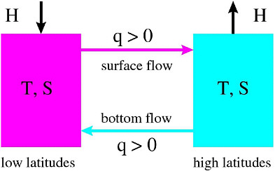 FIGURE 3.2 |
decrease as well but then responds with a sudden transition to the reverse mode. This is an abrupt climate change according to the definition used in this document; the response is considerably faster than the change in forcing.
As for the real Atlantic and climate system, the crucial question is whether the THC is best characterized by the “lower” or by the “upper” case. Is there a possibility that a temporary perturbation in, say, the freshwater forcing can induce a permanent change in the THC? This would
|
Figure 3.2 shows the original set-up of Stommel’s two-box model for the THC. North-south exchange of water between a low-latitude box (left) and a high latitude box (right) is parameterized as a function of the density difference between the two boxes. H denotes the freshwater forcing, the flux of freshwater through the atmosphere from low latitudes to high latitudes or equivalently, as shown here, the flux of salt through the atmosphere from high latitudes to low latitudes. The circulation consists of a volume flux q taken to be proportional to the density difference between high and low latitudes. If q > 0, there is poleward surface flow because high-latitude density is greater than low-latitude density, and vice versa. At low latitudes, the ocean gains heat from and loses freshwater to the atmosphere; the opposite is true at high latitudes. Consequently, both temperature and salinity are higher at low latitudes than at high latitudes. This has opposite effects on density. When q > 0, the temperature difference dominates the density difference and drives the circulation, whereas the salinity difference brakes it, and vice versa. The situation q > 0, with sinking implied at high latitudes, is familiar from the North Atlantic and describes today’s active THC. In a plausible limiting case (Marotzke, 1990), the box temperatures are assumed to be imposed by the atmosphere, as is the surface freshwater exchange. A new addition to the system is horizontal diffusion. It reflects the transport of salinity by the ocean gyres, the systems of ocean circulation characterized by swift currents near the western boundary and slower return flows farther eastward, occurring at virtually the same depth. Understanding the effect of ocean gyres on the stability of the THC is crucial, and the models currently used are likely to distort this influence because of their low spatial resolution. Two cases are considered here. The “standard” case is the classical THC box model with only very weak diffusion; the other case will be designated “diffusive.” In the example shown, the diffusive case has a different proportionality factor relating density differences to flow strength, such that with the same freshwater forcing, the two cases have very similar strengths of the “normal” North Atlantic THC. |
imply that the real THC displays hysteresis and the possibility of abrupt change. Or would any transition be smooth, on the time scale of the forcing change, and be reversible? Simulations with comprehensive three-dimensional GCMs show both types of behavior. An ocean model with relatively large diffusion, caused by the choice of the numerical scheme, exhibits a transient behavior very similar to the upper dashed curve in Figure 3.4 when a slow freshwater flux perturbation is applied to the North Atlantic (Mikolajewicz and Maier-Reimer, 1994). A less-diffusive coupled model
|
Box 3.3 Multiple Equilibria and Model Parameters 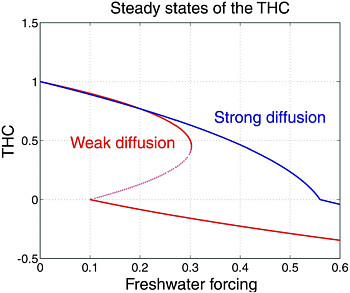 FIGURE 3.3 Steady-state solutions of the two-box model as a function of the atmosphere-ocean freshwater flux H. Depending on the strength of the horizontal mixing (diffusion) the model exhibits multiple eqilibria for a limited range of freshwater fluxes (bottom curve) or, alternatively, a unique solution (top curve). (See plate 6 for more detail.) |
exhibits a permanent change in the THC (Manabe and Stouffer, 1988). This aspect has been associated with the quantitatively different vertical mixing in these models (Manabe and Stouffer, 1999).
The simple box model above demonstrates that the shape and position of the hysteresis in parameter space depend strongly on the model setup and on values of model parameters. Uncertainties in the parameters translate directly into uncertainties in the hysteresis and therefore uncertainties in the likely response of a system to a perturbation. Investigations using simplified models indicate that mixing schemes and values of mixing parameters are crucial in determining the shape of the hysteresis (Knutti and Stocker, 2000; Schmittner and Weaver, 2001). Unfortunately, mixing in the ocean is not well simulated in current-generation climate models, because of poorly parameterized small-scale processes and insufficient resolution. The location of the present, past, and future states of the climate system on the hysteresis curve, and its shape
|
Figure 3.3 (also see Plate 6) shows that the steady states of the two-box model can be calculated analytically and the dependence of the flux q (a measure of the strength of the THC) on the freshwater flux H can be examined. In the standard case (weak diffusion, lower curve), the THC is strongest (value arbitrarily set to 1) when the freshwater flux H vanishes. With higher H, the THC weakens. If H = 0.3, no steady-state solution with q > 0 is possible. However, for H > 0.1, there is a second stable equilibrium, a reverse mode of the THC, with q < 0. This flow pattern strengthens as H increases. For a certain parameter range, here 0.1 < H < 0.3, three equilibria are possible; it is readily shown that the middle one (on the dotted part of the curve) is not a stable solution. In that range of H, the model exhibits hysteresis. The presence of hysteresis is strongly dependent on model parameters. This is shown for a case in which the effect of the horizontal mixing due to gyre transports is increased (strong diffusion). Hysteresis disappears (upper curve); and for progressively increasing freshwater forcing, the THC smoothly approaches zero and—again smoothly—turns into the reverse mode for H = 0.56. For any given freshwater forcing, there is a unique and stable THC. The presence of multiple equilibria of the THC therefore depends strongly on the model formulation, parameterization of processes, and choice of parameter values. |
and complexity, clearly are among the major unsolved problems in climate dynamics. Results that depend crucially on a specific shape of the hysteresis are likely not to be robust findings at this stage.
Whether the nonlinearities giving rise to abrupt change in the simplified models are an artifact of the simplifications or carry over to more complex and realistic systems needs to be investigated. Only more comprehensive and more complete climate models can make a convincing case that the assumptions underlying the nonlinearities in these simple models bear sufficient realism.
Simulation of Past Changes of the Thermohaline Circulation
Earlier, three fundamental ways of causing abrupt climate change were presented; all have been simulated with coupled GCMs. The first category
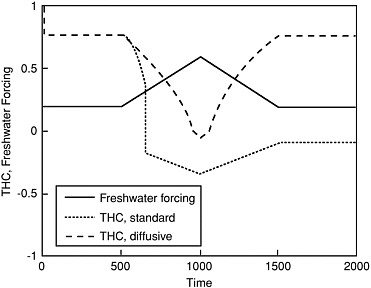
FIGURE 3.4 Response to the thermohaline circulation (THC) to a slow increase and subsequent slow decrease in freshwater forcing for the two cases in Figure 3.3.
concerns the response to a sudden external perturbation, such as a disintegrating ice sheet. Manabe and Stouffer (1995) released a short, strong pulse of freshwater (1 Sv = 106 m3/s for 10 years) into the northern North Atlantic in their coupled model. The THC responded instantaneously with a reduction of almost 70 percent within a decade but recovered to the original strength within less than 200 years. Although the THC shut down almost completely, a threshold was not crossed, and no transition to a new equilibrium was simulated. The model does, however, have a second equilibrium that is achieved if the perturbation is much stronger (Manabe and Stouffer, 1999). It appears, therefore, that the behavior of the model is qualitatively similar to the standard case of the Stommel two-box model (see Plate 6, orange line). Depending on the amplitude of the perturbation, the coupled GCM thus exhibits either a transition to a new stable state or a reversible change (which might still be abrupt and of large amplitude). Manabe and Stouffer (1999) also showed that simply increasing the vertical diffusivity in their model led to a situation with a single equilibrium; this implies that processes other than those discussed above could qualitatively change the hysteresis structure of the model.
Behavior similar to that in Manabe and Stouffer’s (1995) model was observed by Schiller et al. (1997), albeit because of a different forcing. They
forced their model with a freshwater flux qualitatively similar to that in Figure 3.4. This coupled model appears to have a unique equilibrium, and the simulated changes evolve roughly on the time scale of the forcing. Any abruptness in such a model will therefore be generated only through the forcing and not through the dynamics of the model itself. The transient behavior of this complex model is qualitatively comparable with that of the diffusive Stommel model (Figure 3.4, upper dashed curve). The complete, temporary shutdown of the THC causes a massive cooling in the North Atlantic and weak warming in the South Atlantic. The climatic behavior of opposite sign during a full THC shutdown has been termed the bipolar seesaw (Broecker, 1998; Stocker, 1998), and is a phenomenon that was probably active during most of the last glacial period (Blunier and Brook, 2001) (see Plate 2).
The second type of abrupt change in climate models occurs when slow changes in the forcing push the model beyond a threshold and induce a transition to a second equilibrium. This behavior is simulated in ocean-only models that include simplified formulations of the atmosphere (Rahmstorf, 1994, 1995) and in models of reduced complexity (Aeberhardt et al., 2000; Schmittner and Weaver, 2001). Periodic forcing can also trigger abrupt change in a model that has multiple equilibria, provided that the forcing amplitude covers both branches of the hysteresis. Ganopolski and Rahmstorf (2001) showed that weak forcing is sufficient if the model’s hysteresis has a narrow shape. As emphasized earlier, such results are not considered robust, because they depend strongly on the structure of the hysteresis and the location of the initial state on it. Tuning and choices of parameters can strongly influence the transient behavior under a given forcing (Schmittner and Weaver, 2001) (Figure 3.4).
The third possibility for the occurrence of abrupt climate change in model simulations is a spontaneous regime transition similar to the paradigm of the Lorenz (1963) model. This concept has been explored in simplified models (Timmermann and Lohmann, 2000) but was recently also found in a control run of a coupled atmosphere-ocean GCM (Hall and Stouffer, 2001). Annual mean surface air temperature, averaged over a region extending from southwestern Greenland to Iceland, showed natural interannual variability of around ±1°C (Figure 3.5, top). During the 15,000-year integration, one event occurred in which the temperature underwent a rapid decrease of about 4°C within a few decades (Figure 3.5, bottom). The event was triggered by an atmospheric pattern of persistent northwesterly flow in the region. This induced a southwestward Ekman flow in the surface ocean,
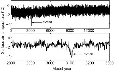
FIGURE 3.5 Model of surface air temperature averaged over an area spanning from southwestern Greenland to Iceland found in a 15,000-year control integration of a coupled atmosphere-ocean Global Circulation Model. The top shows the entire series, while the bottom highlights a 500-year period that contains an abrupt cooling event. (Hall and Stouffer, 2001).
enhanced the East Greenland Current, and brought freshwater into the northern North Atlantic. Only then did the THC respond with a weakening that amplified the initial perturbation. In this example, changes in the THC were a response to rather than a cause of the cooling event. Although the result is intriguing, its robustness is poorly understood; the lack of intermediate-size events during the long integration is a cause for concern.
Some Open Questions
Even if one accepts that the THC played a central role in past abrupt climate change, the above examples of recent studies underline how our understanding of past rapid changes is still limited. In particular, the question of what triggered abrupt climate change, such as the Younger Dryas, has not yet been answered, unless we assume that the climate system essentially exhibits spontaneous regime transitions of the THC. In the following, we attempt to break down that overarching question into smaller, more manageable topics. The problem contains some fundamental aspects, as epitomized by the two different hysteresis structures in Plate 6, indicating that the whole spectrum of approaches—theory, modeling, and observations—will be needed.
The conceptual discussion above has been framed entirely in terms of Stommel’s hemispheric model of the THC, but the likely importance of the bipolar see-saw alone indicates that this view must be broadened. Two seemingly unrelated questions help to focus the discussion: First, what is the role of convective mixing in the THC? Second, if salinity is so important in determining the global THC pattern, why does the North Atlantic gain its high-latitude surface density mainly through heat loss (Schmitt et al., 1989)? The first question is motivated by the strong observational (Munk, 1966; Munk and Wunsch, 1998) and numerical (e.g., Bryan, 1987; Marotzke, 1997) evidence that the strength of the THC is strongly controlled by the vigor of vertical mixing in the stratified regions of the ocean. This is because the deepwater that upwells in these regions must be heated by mixing to maintain the near-surface higher temperatures. In contrast, the THC strength is quite insensitive to the efficiency of convective mixing (that is, the speed with which the ocean eliminates dense water overlying lighter water), and the THC could even be strong in the absence of convective mixing, according to the single-hemisphere GCM of Marotzke and Stott (1999).
The answer to the first question leads the way to answering the second. Marotzke (2000) has argued that the results from single-hemisphere models should be viewed as applying to the global integral of the various THC branches and that the magnitude of the global integral obeys different laws from the distribution of the grand total over various competing deepwater formation sites. A number of idealized and more realistic ocean GCMs have shown that varying the freshwater flux forcing leaves the global integral of deep sinking nearly constant but the strength of North Atlantic sinking considerably changed (Tziperman, 1997; Klinger and Marotzke, 1999; Wang et al., 1999). Hence, a reduction in Northern Hemisphere THC would be associated with an increase in Southern Hemisphere THC. Thus, the globally integrated THC (sum of all branches) is rate-limited by vertical mixing and the gross pole-equator density contrast, which is dominated by the pole-equator temperature contrast (not by salinity). It follows that convection is basically driven by heat loss and that it occurs predominantly at high latitudes.
That so much oceanic deepwater is formed in the North Atlantic, and not in any of the other competing high latitude regions, is determined by the North Atlantic’s high surface salinity and hence high surface density. These, in turn, are strongly influenced by the freshwater flux forcing; moreover,
the deepwater formation is intimately related to the very deep convective mixing occurring there.
This two-step procedure—considering first the global integral of THC strength and then its distribution over different regions—helps to sort out a number of conceptual questions, but others arise. Most important is the role of the Antarctic Circumpolar Current, especially the wind-induced upwelling there (Toggweiler and Samuels, 1995); this has only recently begun to be addressed theoretically (Gnanadesikan, 1999). The interaction of the North Atlantic THC with the other oceans is poorly understood, both conceptually and from observations (e.g., Whitworth et al., 1999).
Extending one’s perspective beyond the Stommel model also calls into question the long-held tenet that freshwater forcing necessarily weakens the THC. Rooth’s (1982) interhemispheric box model suggests that the Atlantic THC actually increases with increased freshwater flux (Rahmstorf, 1996; Scott et al., 1999; Marotzke, 2000). This is confirmed for the Atlantic branch of the THC in an idealized global GCM, as long as one considers the equilibrium response (Wang et al., 1999). Under a faster increase, as would be expected with increased greenhouse gases or might have occurred with outburst floods or ice-sheet surges in the past, the THC did weaken.
If the equilibrium response can be interpreted as reflecting the THC’s response to very slowly varying atmospheric moisture flux, as might plausibly have happened during the glaciations, the assumed overall glacial weakening of the THC, as opposed to the shorter-lived and stronger proposed weakening of the THC in specific events during the glacial, could be explained.
Given confirmation that the North Atlantic surface densities and the resulting convective activity do matter, the question arises whether we understand, and can observe, what they are influenced by. The drivers could be oceanic transports of freshwater (e.g., Aagard and Carmack, 1989) and heat, local surface fluxes, or remote influences, such as the water-vapor transport from the Atlantic to the Pacific (Zaucker and Broecker, 1992; Schmittner et al., 2000; Latif et al., 2000). In addition, one should consider the evolution of surface density in the Southern Ocean, in particular the Weddell Sea, because it is not well observed and the processes that link it with North Atlantic densities are not well understood.
There is a huge gap in our conceptual understanding linking changes in convective activity, in the North Atlantic or elsewhere, to the THC and the northward heat transport. Regionally, changes in properties appear to occur rapidly but are poorly understood (e.g., Sy et al., 1997). On a larger
scale, the THC (and hence heat transport) can respond to changes in external forcing much faster than on the millennial time scale of thermodynamic equilibration of the deep ocean, but it is not clear which of the various plausible, identifiable time scales—ranging from months to decades—is most relevant. The classical picture (Kawase, 1987; Döscher et al., 1994) suggests that the deep circulation is set up through wave processes on time scales of months to a few years, but it has also been argued that advection by the deep western boundary current must be important, and this implies time scales of decades (Marotzke and Klinger, 2000).
The potential predictability and prediction of the THC raise the thorny issue of assessing the quality of numerical simulations of future climate evolution. The fundamental problem is best understood when juxtaposed with daily weather forecasting. Through thousands of forecasts based on model simulations, it has been established that weather predictions have “skill”; that is, they improve upon a naïve baseline. But the time needed to test a weather forecast typically is a day—we will know tomorrow night whether tomorrow’s picnic gets rained out. An analogous accumulation of evidence of forecast skill is impossible when the prediction lead time is decades and more. How, then, can we state with well-defined confidence what is likely in store?
An abrupt THC change is likely to have consequences massive enough that its probability should be estimated, if only crudely. In lieu of establishing true forecast skill, the models used for future climate-change scenarios should pass all the tests posed by available data. For example, one would reasonably have more confidence in climate models of future evolution that were able also to simulate the complicated climate history, including the rapid changes, of the last glacial interval. However, it is difficult to establish the “transferability” of putative modeling success of the past. Although being able to simulate the Younger Dryas is neither strictly necessary nor sufficient for being able to predict the THC’s evolution under global warming, it would enhance confidence considerably. Another strategy would be to simulate an ensemble of possible future climates and ascribe probabilities to them; an example is discussed in Chapter 4. Still, the problem remains of assessing whether the probabilities have the right order of magnitude. A further limit to predictability might arise from chaotic dynamics. In the global model of Wang et al. (1999), the timing and presumably the critical threshold of a THC collapse were fundamentally unpredictable to within a factor of 2. Different realizations of statistically identical random perturbations in the wind field in Wang et al. (1999), mimicking different (unpre-
dictable) weather histories, led to collapse times of that varied between 250 and 500 years. These results have not been confirmed (or challenged) with more sophisticated models, and the random perturbations might have been unrealistically large, but the possibly chaotic nature of THC changes needs to be addressed.
Considering the known limitations of climate models, it is not currently possible to ascribe probabilities to future abrupt climate changes. Given the possible large impacts, simulation of abrupt climate change caused by a collapse in the THC constitutes a “Grand Challenge” problem in computational earth science. A dedicated supercomputer could be used to test whether the THC shows the possibility of threshold behavior, abrupt change, and hysteresis in a climate model that in its ocean components resolves the most important features of the ocean circulation. The conceptual models discussed here demonstrate that the outcome is open: on the one hand, high-resolution models are expected to have stronger gyre transport of heat and salinity, which appears to work in favor of the diffusive paradigm; on the other hand, a high-resolution model would be expected to exhibit a greater degree of internal variability, increasing the chance of self-induced threshold-crossing—if indeed a threshold exists. The need for substantially increased computational resources is clear.


