Making Sense of Complexity: Summary of the Workshop on Dynamical Modeling of Complex Biomedical Systems (2002)

One of the common major goals of the work described in Chapter 2 is the derivation of simple models to help understand complex biological processes. As these models evolve, they not only can help improve understanding but also can suggest aspects that experimental methods alone may not. In part, this is because the mathematical model allows for greater control of the (simulated) environmental conditions. This control allows the researcher to, for example, identify stimulus-response patterns in the mathematical model whose presence, if verified experimentally, can reveal important insights into the intracellular mechanisms.

At the workshop, John Rinzel, of New York University, explained how he had used a system of differential equations and dynamical systems theory to model the neural signaling network that seems to control the onset of sleep. Rinzel’s formulation sheds light on the intrinsic mechanisms of nerve cells, such as repetitive firing and bursting oscillations of individual cells, and the models were able to successfully mimic the patterns exhibited experimentally. More detail may be accessed through his Web page, at <http://www.cns.nyu.edu/corefaculty/Rinzel.html>.

In another approach, based on point processes and signal analysis techniques, Don Johnson, of Rice University, formulated a model for the neural processing of information. When a neuron receives an input (an increase in voltage) on one of its dendrites, a spike wave—a brief, isolated pulse having a characteristic waveform—is produced and travels down the axons to the presynaptic terminals (see Figure 3-1). The sensory information in the nervous system is embedded in the timing of the spike waves. These spikes are usually modeled as point processes; however, these point processes have a dependence structure and, because of the presence of a stimulus, are nonstationary. Thus, non-Gaussian signal processing techniques are needed to analyze data recorded from sensory neurons to determine which aspects of the stimulus correlate with the neurons’ output and the strength of the correlation.

Johnson developed the necessary signal processing techniques and applied them to the neuron spike train (see details in Johnson et al. (2000) and also at <http://www.ece.rice.edu/~dhj/#auditory>). This theory can be extended to an ensemble of neurons receiving the same input, and under some mild assumptions the information can be measured with increasing precision as the ensemble size increases.

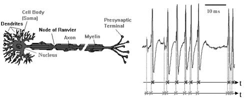
FIGURE 3-1 Neural representation of information. Information is represented by when spikes occur, either in single-neuron responses or, more importantly, jointly, in population (ensemble) neural responses. A theoretical framework is needed for analyzing and predicting how well neurons convey information. Figure courtesy of Don Johnson.

Larry Abbott, of Brandeis University, also explored the characteristics of neuron signals. He presented research on the effect of noise as an excitatory input to obtain a neural response, and his methods took advantage of the difference between in vivo measurements and in vitro measurements. His work counters one of the most widespread misconceptions, that conductance alone changes the neural firing rate. Instead, a combination of conductance and noise controls the rate. As Figure 3-2 shows, although a constant current produces a regular spike train in vitro, this does not happen in vivo, where there is variance in the response, and thus more noise in the signal.

It is of great interest to study the input and output relations in a single neuron, which has more than 10,000 excitatory and inhibitory inputs. Let I denote the mean input current, which measures the difference between activation and inhibitory status, and let σ_I² be the input variance. For an output with a mean firing rate of r hertz, neuroscientists typically study the output’s variance σ_v² and coefficient of variation CV. Abbott also studies how the mean firing rate changes as the mean input current varies; this is labeled as the “gain,” dr/dl, in Figure 3-3. The standard view is as follows:

• The mean input current I controls the mean firing rate r of the output.

• The variance of the input current affects σ_v² and CV.

Abbott disputes the second statement and concludes that the noise channel also carries information about the firing rate r. To examine this dispute, Abbott carried out in vitro and in vivo current injection experiments.

In the first experiment, an RC circuit receiving constant current was studied. Such a circuit can be represented with a set of linear equations that can be solved analytically. The result from this experiment showed that the output variance increases as input variance increases, and that it reaches an asymptote at large σ_I². The firing rate r increases as the input I increases, and the CV decreases as r increases.

Abbott’s second experiment studied real neurons in an artificial environment: Laboratory-generated signals were used as the input to actual neurons in vivo (see Figure 3-4). Both excitatory and

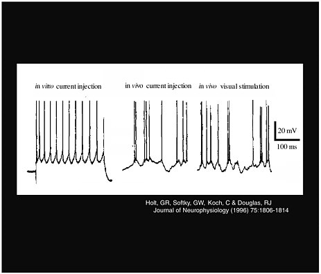
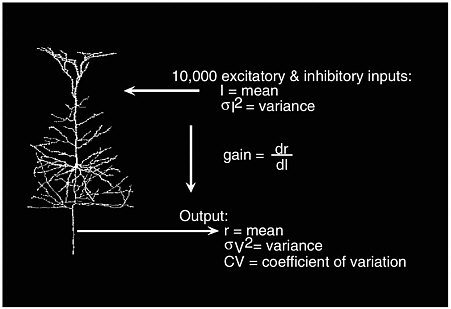
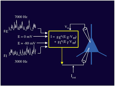
FIGURE 3-4 Neural stimuli. Figure courtesy of Larry Abbott.

inhibitory inputs (g_E and g_I), at different voltages, combine to create the input I that is fed into the neuron (triangle in Figure 3-4). Through this experiment it was shown that the mean of the input affects the rate but that the variance of the input is not correlated with the variance of the output. Instead, the input variance acts more like a volume control for the output, affecting the gain of the response. Dayan and Abbott (2001) contains more detail on this subject.

The workshop’s last foray into neuroscience was through the work of Emery Brown, of the Harvard Medical School, whose goal was to answer two questions:

• Do ensembles of neurons in the rat hippocampus maintain a dynamic representation of the animal’s location in space?

• How can we characterize the dynamics of the spatial receptive fields of neurons in the rat hippocampus?

The hippocampus is the area in the brain that is responsible for short-term memory, so it is reasonable to assume that it would be active when the rat is in a foraging and exploring mode. For a given location in the rat’s brain, Brown postulated that the probability function describing the number of neural spikes would follow an inhomogeneous Poisson process:

Prob(k spikes) = e^-λ(t⁾λ(t) k/k!

where λ(t) is a function of the spike train and location over the time interval (0, t). (Brown later generalized this to an inhomogeneous gamma distribution.) Given this probability density of the

number of spikes at a given location, we next assume that the locations x(t) vary according to a Gaussian spatial intensity function given by

where µ is the center, W is the variance matrix, and exp{α} is a scaling constant.

This model was fit to data, and an experiment was run to see how it performed. In the experiment, a rat that had been trained to forage for chocolate pellets scattered randomly in a small area was allowed to do so while data on spike and location were recorded. The model was then used to predict the location of brain activity and validated against the actual location. The agreement was reasonable, with the Poisson prediction interval covering the actual rate of activation 37 percent of the time and the inhomogeneous gamma distribution covering it 62 percent of the time. Brown concluded that the receptive fields of the hippocampus do indeed maintain a dynamic representation of the mouse’s location, even when the mouse is performing well-learned tasks in a familiar environment, and that the model, using recursive state-space estimation and filtering, can be used to analyze the dynamic properties of this neural system. More information about Brown’s work may be found at <http://neurostat.mgh.harvard.edu/brown/emeryhomepage.htm>.