
A
Statistical Details
MIXTURE MODELS
One can naturally model the unobserved population heterogeneity or extra-population heterogeneity via mixture models. The simplest and most natural occurrence of the mixture model arises when one samples from a super population g which is a mixture of a finite number, say m, of populations (g1,…, gm), called the components of the population. Suppose a sample from a super population g is recorded as data (Yi, J i) for i = 1, …, n, where Yi = yi is a measurement on the ith sampled unit and Ji = ji indicates the index number of the component to which the unit belongs. If sampling is done from the jth component, an appropriate probability model for the sampling distribution is given by
P(Yi = yi|Ji = j) = fj(yi; θj)
The function fj(yi; θj) represents a density function, called the component density for the ith observation yi and the parameter θj![]() Θj
Θj![]()
![]() dj called the component parameter, that describes the specific attributes of the jth component population, gj.
dj called the component parameter, that describes the specific attributes of the jth component population, gj.
We treat the Ji as missing data and define the latent random variable Φ= (Ф1,…, Фn) to be the values of the parameter θ ![]() {θ1, …,θm} corresponding to the sampled components J1, …, Jn; i.e., if the ith observation came from the jth component, then define Фi = θj. Then the Фi are a random sample from the discrete probability measure Q that assigns a positive probability πj to the support point θj for j = 1, …, m. That is, the latent
{θ1, …,θm} corresponding to the sampled components J1, …, Jn; i.e., if the ith observation came from the jth component, then define Фi = θj. Then the Фi are a random sample from the discrete probability measure Q that assigns a positive probability πj to the support point θj for j = 1, …, m. That is, the latent
random variable Φ has a distribution Q, which is called the mixing distribution, defined by P(Φ =θj) = Q({θj }) = πj. Thus the mixing distribution
puts a mass (or weight) of πj on each parameter θj. We thus arrive at the mixture distribution ![]() , or equivalently
, or equivalently
One can find the posterior probability that the ith observation comes from the jth component (i.e, yi![]() Gj) using
Gj) using
In turn, one can assign each yi to the population to which it has the highest estimated posterior probability of belonging; i.e., to gj if τij > τit for t = 1, …, m and t ≠ j.
Estimation of the Parameters and the Mixture Components
One has to estimate the number of subpopulations or number of mixture components m as well as the parameters in the mixture distribution g…). This can be achieved via parametric or non-parametric maximum likelihood estimation (Laird, 1978; Böhning et al. 1992, Pilla and Lindsay, 2001). Laird (1978) considered nonparametric likelihood estimation of a mixing distribution and Lindsay (1983) linked its general theory, developed from a study of the geometry of the mixture likelihood, to the problem of estimating a discrete mixing distribution. One may also use an alternative approach to maximum likelihood for which menu driven software is provided by Böhning et al. (1998).
For a given m, one can estimate the parameters in the mixture distribution via the EM algorithm (Dempster et al. 1977) and several improvements of it which are discussed in McLachlan and Krishnan (1997). Let ![]() = (
= ( ![]() ,
, ![]() ) be the vector of estimated parameters. Once
) be the vector of estimated parameters. Once ![]() has been obtained, estimates of the posterior probability of population membership
has been obtained, estimates of the posterior probability of population membership ![]() ij can be formed for each yi to give a probabilistic clustering.
ij can be formed for each yi to give a probabilistic clustering.
When m, the number of mixtures, is large, the EM algorithm can be excruciatingly slow. In that case, one can use alternative EM methods proposed by Pilla (1997) and Pilla and Lindsay (2001) in the nonparamet-
ric mixture setting. Their approach assumes that the θ’s are known and the goal is to estimate the π’s only. However, by setting up the problem in a nonparametric framework, one may find the maximum likelihood estimator (MLE) quite easily in a high-dimensional problem via Pilla and Lindsay’s method. These methods are especially useful because θ1 < θ2 < …, i.e., the support points are ordered and hence the corresponding nearby densities can be paired to take advantage of the correlated densities.
Mixture Setting for Detecting Spatial Occurrence of Suicide
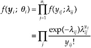
Suppose data are available on the spatial occurrence of suicide in N counties in a state or for the entire country over a five year period. Assume that the counties are a mixture of two groups g1 and g2, corresponding to normal and high risk with respect to suicide, in proportions of π1 and π2 respectively. The number of events yi in the ith county is assumed to have a Poisson distribution with a rate of μj in gj for j = 1, 2; i= 1, …, n. Let ![]() = (μ1, μ2, π1, π2)T and θi = (μ1Ni, μ2Ni)T, where Ni= Miti is the mass of population at risk in the ith county assuming that there are Mi individuals at risk over time ti. In this scenario, the log likelihood becomes
= (μ1, μ2, π1, π2)T and θi = (μ1Ni, μ2Ni)T, where Ni= Miti is the mass of population at risk in the ith county assuming that there are Mi individuals at risk over time ti. In this scenario, the log likelihood becomes
where fj(yi; θi) = exp(–μjNi) (μjNi)yi/yi!. One can use the EM algorithm to find the MLE of the parameters. The complete data log likelihood function becomes
where zij = 1 if yi![]() gj and 0 otherwise. The MLE of the parameters are found iteratively via
gj and 0 otherwise. The MLE of the parameters are found iteratively via
and
where ![]() which is the estimated posterior probability that yi
which is the estimated posterior probability that yi![]() gj.
gj.
Testing for the Number of Components in a Mixture
Testing for the number of components in a mixture is a very hard problem. Consider the problem of testing the hypothesis H0: number of components = m against H0: number of components = m + 1. The likelihood ratio test (LRT) statistic defined as 2 log Ln = 2 [l(![]() m) – l(
m) – l(![]() m+1)], where l(
m+1)], where l(![]() m) is the log likelihood log
m) is the log likelihood log ![]() evaluated at
evaluated at ![]() m, the nonparametric MLE under H0 and similarly l(
m, the nonparametric MLE under H0 and similarly l(![]() m+1) is the nonparametric MLE under H1. The LRT statistic generally has an asymptotic χ2 distribution with d degrees of freedom, where d equals the difference between the number of parameters under the alternative and null hypothesis. However, this theory is known to fail for the mixture problem (Titterington et al., 1985:154). The reason for this is that the null hypothesis does not lie in the interior of the parameter space. The problem is not yet solved except for some special cases. However, the simulations or bootstrap can shed some light on the distributional properties of the LRT. See Lindsay (1995) and Böhning (1999) (including the references therein) for recent developments in theory and methods to test for the number of components in a mixture. There are other techniques for identifying the number of components of a mixing distribution including a variety of graphical techniques (Lindsay and Roeder, 1992).
m+1) is the nonparametric MLE under H1. The LRT statistic generally has an asymptotic χ2 distribution with d degrees of freedom, where d equals the difference between the number of parameters under the alternative and null hypothesis. However, this theory is known to fail for the mixture problem (Titterington et al., 1985:154). The reason for this is that the null hypothesis does not lie in the interior of the parameter space. The problem is not yet solved except for some special cases. However, the simulations or bootstrap can shed some light on the distributional properties of the LRT. See Lindsay (1995) and Böhning (1999) (including the references therein) for recent developments in theory and methods to test for the number of components in a mixture. There are other techniques for identifying the number of components of a mixing distribution including a variety of graphical techniques (Lindsay and Roeder, 1992).
The Choice of Initial Values and Multiple Mode Problem for the EM Algorithm
The continuous EM algorithm that finds the MLE of parameter estimators, for a given m, requires the specification of initial values for the number and location of the support points. Pilla and Lindsay (2001) show that if the number of support points is fixed in advance, then one could have multiple modes whereas the nonparametric ML approach corresponds to a unimodal likelihood. Böhning (1999) illustrates through an example where the choice of initial values is critical; for example, in testing for the number of components in the mixture. Through simulations, he demonstrates the effectiveness of several approaches that combat this problem. His recommendation is to choose the support points as values of certain order statistics of the data (see Böhning, 1999:68–70). In his simulation studies, the gold standard (the grid approach given below) seems to outperform the other methods. The optimization problem solved by the grid-based EM (where the support points are assumed known) proposed by Pilla and Lindsay (2001) has a unique optimum which in turn generates an estimated number of components. However, the continuous EM can converge to the suboptimal mode.
In light of the above characteristics, Pilla and Lindsay (2001) suggest the following: to obtain a continuous solution with a flexible number of support points, first start with one of the fast EM-based algorithms proposed by Pilla and Lindsay on a grid and next use the resulting solution as starting values for the continuous EM. This will protect against using an incorrect number of points or finding suboptimal solutions.
Convergence Criteria
Finding a natural stopping rule for iterative algorithms in the mixture problem when the final log likelihood is unknown is an important problem. In a potentially slow algorithm like EM, a far weaker convergence criterion based on the changes in the log likelihood value or on changes in the parameter estimates between iterations can be very misleading (Titterington et al. 1985:90). See Lindsay (1995:62–63) for further details. The following gradient-based stopping criterion proposed by Lindsay (1995:131–132) can be used to detect the convergence of the EM algorithm: we stop when sup DQ(θ) ≤ ε, with ε = 0.005, where the gradient function DQ(θ) is defined as
then we automatically satisfy the ‘ideal stopping criterion’: |log Lobs(![]() ; y) – log Lobs(
; y) – log Lobs(![]() p; y)| ≤ ε, where
p; y)| ≤ ε, where ![]() p is the estimate at the pth iteration. The gradient function therefore creates a natural stopping rule for iterative algorithms such as the EM when the final log likelihood is unknown, although it is more stringent than the ideal stopping rule.
p is the estimate at the pth iteration. The gradient function therefore creates a natural stopping rule for iterative algorithms such as the EM when the final log likelihood is unknown, although it is more stringent than the ideal stopping rule.
Illustration of Poisson Mixture Model
To illustrate use of the Poisson mixture model we analyzed countylevel suicide data for the US for the time period of 1996–1998. The three year period was used to obtain more stable estimates of the parameters. Application of the Poisson mixture model identified a mixture of four component distributions with proportions of .1125, .4523, .3119, and .1234, and means of 7.5, 10.9, 14.9, and 20.6 suicides per 100,000. Results of classifying counties into component distributions are displayed in Figure 1. Inspection of the map in Figure 1 reveals that those counties classified in the highest component distribution (20.6 suicides per 100,000), are predominantly in the western states with lowest population density, although there are exceptions throughout the country (see Figure A-1). Counties classified in the lowest component distribution (7.5 suicides per 100,000)
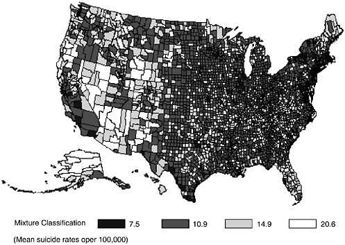
FIGURE A-1 Annual Suicide Rates per 100,000 (1996–1998). The Poisson Mixture Model applied to county-level data.
appear to be clustered in the central United States. Finally, counties classified into the two intermediate groups are largely in the eastern portion of the United States. Unlike the earlier attempt at fitting a mixture distribution to temporal suicide data collected in Cook county (Gibbons et al., 1990) that was designed to identify “suicide epidemics” and failed to do so, the results of this analysis has focused on the spatial distribution of suicide and has identified qualitatively distinct geographic groupings of suicide rates across the United States. Note that this mixture distribution does not adjust for demographic disparity across the counties (e.g., age, sex, race, population density, etc.) that may have produced the mixture distribution in the first place.
POISSON REGRESSION MODELS
In the following sections, we present statistical details of both fixed-effects and mixed-effects Poisson regression models.
Fixed-Effects Poisson Regression Model
In Poisson regression modeling, the data are modeled as Poisson counts whose means are expressed as a function of covariates. Let yi be a response variable and xi = (1, xi1,…, xip)T be a [(p+1) × 1] vector of covariates for the ith individual. Then the Poisson regression model yi is
(2)
where λ i = exp(βTxi) and β = (β0, β1, …, βp)T is a (p+1)-dimensional vector of unknown parameters corresponding to xi. An important property of the Poisson distribution is the equality of the mean and variance:
E(yi) = Var(yi) = λi
(3)
From equation (2) one can write the likelihood and the log likelihood functions for the n independent observations as
and
respectively. The first and second partial derivatives with respect to the unknown parameters β are given by
and
respectively. Since the above equations are not linear, iterative procedures such as the Newton-Raphson algorithm or Fisher’s scoring algorithm are used to obtain the MLE of β, denoted by ![]() . A consistent estimator of the variance-covariance matrix of
. A consistent estimator of the variance-covariance matrix of ![]() , V(
, V(![]() ) is the inverse of the information matrix, I(
) is the inverse of the information matrix, I(![]() ) — which is the negative of inverse of the matrix of second partial derivatives evaluated at the MLE. Inferences on the regression parameter β can be made using V(
) — which is the negative of inverse of the matrix of second partial derivatives evaluated at the MLE. Inferences on the regression parameter β can be made using V(![]() ).
).
Mixed-Effects Poisson Regression Model
When we have a mixture of fixed and random effects, the more general mixed-effects Poisson regression model is used. Suppose that there are n = Σini nonnegative observations yij for i = 1, …, nc clusters and j = 1, …, ni observations and a (p + 1) dimensional unknown parameter vector, β, associated with a covariate vector xij = (1, xij1, …, xijp)T. Further, let the random effect υi be normally-distributed with mean 0 and variance σ2 and independent of the covariate vector xij. Then the conditional density function, f(yi; θi), of the ni suicide rates in cluster i is written as:
(4)
with
λij =exp(βTxij + υi )
=exp(βTxij + σθi ),
where θi = υi/σ such that θi ~N (0,1). Thus the log-likelihood function corresponding to equation 4 becomes
The first and second derivatives of log L with respect to β and σ are
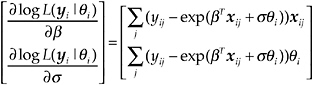
and
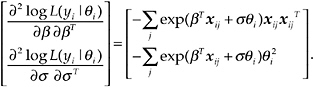
The marginal density of yi can be written as
where g(θ) represents the multivariate standard normal density. One can approximate the above integral via the Gaussian quadrature as
(5)
where λijq = exp(βTxij + σBq), Bq is the quadrature node and A(Bq) is the corresponding quadrature weight. From equation (5), one can obtain the first derivatives of the approximate log likelihood as
and
Solution of the above likelihood equations can be obtained iteratively using the Newton-Raphson algorithm. On the ith iteration, estimates for a parameter vector Θ are given by
(6)
where ![]() is the matrix of second derivatives of the log-likelihood, evaluated at Θi. Alternatively, one can use the Fisher scoring method. This method replaces the matrix of second derivatives in (6) by their expected values:
is the matrix of second derivatives of the log-likelihood, evaluated at Θi. Alternatively, one can use the Fisher scoring method. This method replaces the matrix of second derivatives in (6) by their expected values:
which is equal to the negative of the information matrix. The scoring solution is often used in cases where the matrix of second derivatives is difficult to obtain. Note that when the expected value and the actual value of the Hessian matrix coincide, the Fisher scoring method and the Newton-Raphson method reduce to the same algorithm.
The convergence of the iterative procedure depends on the initial values of the parameters. Good starting values reduce the number of iterations needed to reach the final estimates. It is sometimes possible that a poor choice of starting values may reach some local maximum instead of the global maximum. For this reason, it is often desirable to re-estimate the parameters under a variety of starting values, or to use the EM algorithm to obtain starting values that are reasonably close to the final solution (Hedeker and Gibbons, 1994).
Estimation of Random Effects
Often, it is of interest to estimate values of the random effects θi within a sample. For this purpose the expected “a posteriori” (EAP) or empirical Bayes estimator ![]() i has been suggested by Bock and Aitkin (1981). The estimator
i has been suggested by Bock and Aitkin (1981). The estimator ![]() i given yi for cluster i can be obtained as:
i given yi for cluster i can be obtained as:
Similarly, the variance of the posterior distribution of ![]() i, which may be used to make inferences regarding the EAP estimator (i.e., the posterior variance is an estimate of precision of the estimate of
i, which may be used to make inferences regarding the EAP estimator (i.e., the posterior variance is an estimate of precision of the estimate of ![]() i), is given by
i), is given by
Generalized Estimating Equations - GEE
An alternative approach to the analysis of clustered suicide rate data is based on Generalized estimating equations (GEEs) models, which were introduced by Liang and Zeger (1986) and Zeger and Liang (1986).
Let yij be the jth response for the ith unit (e.g., county ) for i = 1, …, nc and j =1, …, ni observations and xij = (1, xij1, …, xijp ) be a vector of covariates for the ith unit. Let yi be the vector of the responses for the ith unit with corresponding mean vector μi and let Vi be an estimate of the covariance matrix of yi. Then the GEE marginal model for estimating β is given by
(7)
and
g(μij) = g(E(y)) =β'xij
(8)
where g is the link function. Common choice for the link function might be the identity link for continuous data, log link for count data, and logit link for binary data. For example, the link functions for the Poisson and logistic regression models are g(a) = log(a) and g(a) = log(a/(1 – a)), respectively.
In addition to the marginal model, the covariance structure of the correlated observations for a given unit of yi is modeled as
(9)
where Ai is a diagonal matrix of variance functions and R(a) is the working correlation matrix of yi specified by the vector of parameters a. Various types of working correlation structures such as exchangeable or autoregressive can be used in the model.
The maximum likelihood estimator ![]() can be obtained by solving the above estimating equations iteratively:
can be obtained by solving the above estimating equations iteratively:
(10)
Illustration of Poisson Regression Model
Returning to the national suicide data from the previous section, we now illustrate how Poisson regression models can be used to estimate the effects of age, race, and sex on clustered (i.e., within counties) suicide rate data. For the purpose of illustration, we considered the effects of age divided into five categories (5-14, 15-24, 25-44, 45-64, and 65 and older), sex, and race (African American versus Other) in the prediction of suicide rates across the U.S. for the period of 1996-1998. These categories were used so that there would be sufficient sample sizes available to compare observed and expected annual suicide rates for both GEE and mixed-effects (maximum marginal likelihood - MMLE) Poisson regression models. To this end, we fit a Poisson regression model with all main effects and two-way interactions using both GEE and a full likelihood mixed-effects model. Given the large sample sizes almost all terms in the model were statistically significant although of widely varying effect sizes. Table 2 displays a comparison of parameter estimates and standard errors for the GEE and mixed-effects models. In general, the GEE and MMLE parameter estimates were remarkably similar. The only nonsignificant terms were two terms in the race by age interaction. The comparison of rates for ages 5-14 versus 15-24 and 5-14 versus 25-44, did not depend on race.
Based on the parameter estimates in Table A-1, we estimated marginal suicide rates for both GEE and mixed-effects models. Table A-2
TABLE A-1 Comparison of Maximum Marginal Likeihood (MMLE) and Generalized Estimating Equations (GEE) for the Clustered Poisson Regression Model
|
|
MMLE |
GEE |
||||
|
Effect |
Estimate |
SE |
Prob |
Estimate |
SE |
Prob |
|
Intercept |
–4.331 |
0.040 |
<0.0001 |
–4.408000 |
0.048000 |
<0.0001 |
|
Female |
–1.009 |
0.076 |
<0.0001 |
–1.009000 |
0.073000 |
<0.0001 |
|
Black vs Other |
–0.292 |
0.103 |
0.0046 |
–0.279000 |
0.112000 |
0.0127 |
|
15–24 vs 05–14 |
2.788 |
0.041 |
<0.0001 |
2.787000 |
0.043000 |
<0.0001 |
|
25–44 vs 05–14 |
3.030 |
0.040 |
<0.0001 |
3.021000 |
0.043000 |
<0.0001 |
|
45–64 vs 05–14 |
2.971 |
0.041 |
<0.0001 |
2.975000 |
0.046000 |
<0.0001 |
|
65+ vs 05–14 |
3.371 |
0.041 |
<0.0001 |
3.390000 |
0.047000 |
<0.0001 |
|
Female x Black |
–0.345 |
0.036 |
<0.0001 |
–0.345000 |
0.041000 |
<0.0001 |
|
Female x 15–24 |
–0.664 |
0.080 |
<0.0001 |
–0.663000 |
0.077000 |
<0.0001 |
|
Female x 25–44 |
–0.355 |
0.077 |
<0.0001 |
–0.357000 |
0.074000 |
<0.0001 |
|
Female x 45–64 |
–0.223 |
0.077 |
0.0038 |
–0.223000 |
0.075000 |
0.0029 |
|
Female x 65+ |
–0.938 |
0.078 |
<0.0001 |
–0.945000 |
0.078000 |
<0.0001 |
|
Black x 15–24 |
0.065 |
0.106 |
0.5434 |
0.068000 |
0.107000 |
0.5297 |
|
Black x 25–44 |
–0.139 |
0.105 |
0.1829 |
–0.141000 |
0.107000 |
0.1877 |
|
Black x 45–64 |
–0.473 |
0.107 |
<0.0001 |
–0.486000 |
0.111000 |
<0.0001 |
|
Black x 65+ |
–0.740 |
0.112 |
<0.0001 |
–0.748000 |
0.117000 |
<0.0001 |
|
County Variance |
0.280 |
0.003 |
<0.0001 |
|
||
displays observed and expected annual suicide rates for both methods of estimation, broken down by age, sex, and race. Inspection of Table A-2 reveals several interesting results. In general, suicide increases with age, is higher in males, and is lower in African Americans. Black females have the lowest suicide rates across the age range. In white males, the suicide rate is increasing with age whereas in all other groups, the suicide rate either is constant or decreases after age 65. Comparison of the expected frequencies for the GEE and mixed-effects models reveal that they are quite similar and the GEE does a slightly better job of recovering the observed marginal rates.
A special feature of the mixed-effects model is the ability of estimating county-specific rates using empirical Bayes estimates of the random effects as described in the previous section. Using these estimates, we can accomplish two goals. First, we can estimate county-specific expected suicide rates, which directly incorporate the effects race, sex, and age of that county. Table A-3 provides a comparison of observed and expected numbers of suicides (1996-1998) for 100 randomly selected counties. In-
TABLE A-2 Observed and Expected Suicide Rates by Age, Race, and Sex. Data: CMF 1996–1998
spection of Table A-3 reveals remarkably close agreement between observed and expected numbers of suicides.
Second, we can use the Bayes estimates directly to obtain county-level suicide rates adjusted for the effects of race, sex, and age. In the case of a Poisson model, the Bayes estimate for a given county is a multiple of the national suicide rate adjusted for the case mix in that county (i.e., race, sex and age). For example, a Bayes estimate of 1.0 represents an adjusted rate that is equal to the national rate. By contrast, a Bayes estimate of 2.0 represents a doubling of the national rate, and a Bayes estimate of 0.5 represents one-half of the national rate. Figure A-2 displays the Bayes estimates by county across the U.S. Inspection of Figure A-2 reveals that even after accounting for these important demographic variables, considerable spatial variability remains. Again, the highest adjusted rates are typically found in the less densely populated areas of the western U.S.
The map in Figure A-2 also provides a useful tool for qualitative research into the etiology of suicide. A natural approach is to examine the
TABLE A-3 Observed and Expected Number of Suicides for 100 Randomly Selected Counties
|
State |
County |
Observed # of Deaths |
Expected # of Deaths |
State |
County |
Observed # of Deaths |
Expected# of Deaths |
|
56 |
7 |
16 |
10.3 |
51 |
75 |
5 |
5.9 |
|
53 |
63 |
169 |
170.4 |
20 |
159 |
6 |
4.5 |
|
5 |
91 |
14 |
13.6 |
21 |
103 |
14 |
8.7 |
|
47 |
111 |
13 |
9.4 |
40 |
45 |
1 |
1.6 |
|
54 |
93 |
1 |
2.8 |
31 |
61 |
1 |
1.5 |
|
28 |
5 |
9 |
5.5 |
31 |
91 |
0 |
0.3 |
|
27 |
141 |
22 |
21.7 |
40 |
73 |
9 |
6.3 |
|
38 |
47 |
0 |
1.0 |
20 |
203 |
1 |
1.0 |
|
21 |
59 |
25 |
27.5 |
1 |
5 |
8 |
8.2 |
|
48 |
451 |
54 |
50.2 |
38 |
51 |
0 |
1.4 |
|
48 |
87 |
3 |
1.4 |
38 |
39 |
2 |
1.3 |
|
18 |
97 |
391 |
385.3 |
21 |
95 |
11 |
12.0 |
|
35 |
7 |
8 |
6.2 |
48 |
73 |
32 |
25.8 |
|
48 |
383 |
2 |
1.5 |
23 |
11 |
38 |
39.6 |
|
31 |
41 |
3 |
4.3 |
55 |
101 |
58 |
59.5 |
|
18 |
7 |
2 |
3.4 |
17 |
107 |
9 |
10.8 |
|
45 |
61 |
6 |
5.9 |
47 |
127 |
1 |
1.9 |
|
19 |
1 |
4 |
3.4 |
55 |
55 |
28 |
28.1 |
|
8 |
119 |
13 |
9.9 |
21 |
223 |
5 |
3.4 |
|
36 |
3 |
22 |
20.9 |
30 |
97 |
1 |
1.4 |
|
19 |
93 |
2 |
2.9 |
19 |
51 |
2 |
3.0 |
|
12 |
95 |
303 |
314.1 |
47 |
129 |
4 |
6.4 |
|
49 |
49 |
89 |
91.1 |
48 |
9 |
2 |
3.0 |
|
28 |
45 |
30 |
24.1 |
19 |
5 |
9 |
6.7 |
|
18 |
107 |
19 |
16.9 |
28 |
69 |
3 |
3.0 |
|
5 |
1 |
6 |
6.8 |
46 |
19 |
6 |
4.1 |
|
17 |
167 |
64 |
64.8 |
27 |
171 |
31 |
30.8 |
|
39 |
89 |
43 |
44.7 |
28 |
53 |
1 |
2.4 |
|
28 |
1 |
9 |
9.5 |
20 |
31 |
2 |
3.1 |
|
53 |
23 |
0 |
0.9 |
51 |
47 |
18 |
15.0 |
|
48 |
213 |
30 |
28.8 |
46 |
123 |
3 |
2.7 |
|
55 |
107 |
9 |
7.1 |
12 |
81 |
135 |
129.6 |
|
31 |
177 |
6 |
6.7 |
2 |
122 |
22 |
20.4 |
|
17 |
49 |
12 |
12.2 |
21 |
61 |
0 |
3.4 |
|
55 |
75 |
18 |
17.5 |
21 |
25 |
7 |
6.3 |
|
8 |
55 |
3 |
2.7 |
26 |
13 |
6 |
4.0 |
|
29 |
121 |
4 |
5.4 |
18 |
157 |
42 |
44.1 |
|
40 |
125 |
34 |
30.2 |
21 |
165 |
2 |
2.2 |
|
20 |
73 |
3 |
3.2 |
48 |
447 |
2 |
0.8 |
|
21 |
109 |
7 |
5.5 |
13 |
265 |
3 |
0.6 |
|
29 |
197 |
2 |
1.8 |
2 |
100 |
2 |
1.0 |
|
51 |
133 |
7 |
5.0 |
55 |
11 |
4 |
5.2 |
|
29 |
105 |
8 |
10.0 |
48 |
81 |
0 |
1.3 |
|
47 |
181 |
14 |
9.7 |
21 |
229 |
6 |
4.6 |
|
51 |
103 |
9 |
5.5 |
55 |
35 |
32 |
32.3 |
|
16 |
15 |
3 |
2.2 |
39 |
151 |
112 |
113.5 |
|
38 |
55 |
2 |
3.5 |
28 |
89 |
17 |
18.4 |
|
39 |
17 |
91 |
93.6 |
19 |
167 |
4 |
8.2 |
|
55 |
51 |
3 |
2.8 |
23 |
27 |
17 |
15.7 |
|
19 |
119 |
3 |
4.2 |
38 |
1 |
0 |
1.1 |
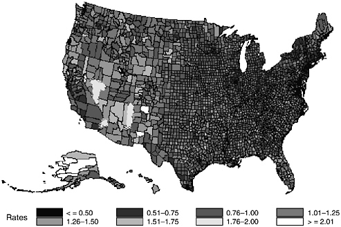
FIGURE A-2 Bayes Estimates of County-Level Deviations from the National Suicide Rates per 100,000 (1996–1998), Adjusted for Age, Sex, and Race.
spatial distribution of Bayes estimates in Figure A-2 for outliers. For example, in the western U.S. and Alaska where suicide rates are typically high there are a few counties that have Bayes estimates that are consistent with the national average. Similarly, in the central U.S. where there is a high concentration of counties with the lowest suicide rates, there are a few counties that exhibit the highest suicide rates. As an example, Table A-4 displays the Bayes estimates, observed and expected numbers of suicides and suicide rates for all counties in Alaska and New Mexico and the 8 counties with estimated adjusted suicide rates less than or equal to half of the national average (national average is 12.33 suicides per 100,000 during the period of 1996–1998). Table A-4 reveals that although there are generally elevated suicide rates in Alaska and New Mexico relative to the national average, there are several counties with low rates, similar to the national average. What are the protective factors that have produced these spatial anomalies? Are these spatial anomalies simply due to reporting bias or some other unmeasured characteristic that has produced the outlying Bayes estimate. Examining these spatial anomalies in greater detail is certainly a fruitful area for further research.
TABLE A-4 Observed and Expected rates per 100,000 for Alaska, New Mexico, and Counties with BE <= 0.50
|
State |
County Name |
Observed # of Suicides |
Expected # of Suicides |
|
ALASKA |
ALEUTIANS EAST |
1 |
0.84 |
|
ALASKA |
ALEUTIANS WEST |
2 |
1.92 |
|
ALASKA |
ANCHORAGE |
118 |
115.66 |
|
ALASKA |
BETHEL |
22 |
10.17 |
|
ALASKA |
BRISTOL BAY |
1 |
0.58 |
|
ALASKA |
DILLINGHAM |
4 |
1.46 |
|
ALASKA |
FAIRBANKS NORTH STAR |
52 |
46.63 |
|
ALASKA |
HAINES |
2 |
0.96 |
|
ALASKA |
JUNEAU |
13 |
11.95 |
|
ALASKA |
KENAI PENINSULA |
22 |
20.38 |
|
ALASKA |
KETCHIKAN GATEWAY |
4 |
4.91 |
|
ALASKA |
KODIAK ISLAND |
5 |
5.17 |
|
ALASKA |
LAKE AND PENINSULA |
4 |
0.63 |
|
ALASKA |
MATANUSKA-SUSITNA |
29 |
25.80 |
|
ALASKA |
NOME |
14 |
5.02 |
|
ALASKA |
NORTH SLOPE |
10 |
3.35 |
|
ALASKA |
NORTHWEST ARCTIC |
15 |
3.87 |
|
ALASKA |
PRINCE OF WALES-OUTER |
3 |
2.64 |
|
ALASKA |
SITKA |
6 |
3.71 |
|
ALASKA |
SKAGWAY-HOONAH-ANGOON |
1 |
1.34 |
|
ALASKA |
SOUTHEAST FAIRBANKS |
6 |
2.69 |
|
ALASKA |
VALDEZ-CORDOVA |
1 |
3.31 |
|
ALASKA |
WADE HAMPTON |
18 |
4.37 |
|
ALASKA |
WRANGELL-PETERSBURG |
8 |
3.73 |
|
ALASKA |
YAKUTAT |
0 |
0.29 |
|
ALASKA |
YUKON-KOYUKUK |
16 |
5.91 |
|
ILLINOIS |
MC LEAN |
17 |
25.62 |
|
NEW JERSEY |
HUNTERDON |
13 |
22.23 |
|
NEW JERSEY |
MORRIS |
80 |
88.20 |
|
NEW JERSEY |
UNION |
80 |
88.66 |
|
NEW MEXICO |
BERNALILLO |
303 |
295.93 |
|
NEW MEXICO |
CATRON |
1 |
1.18 |
|
NEW MEXICO |
CHAVES |
24 |
23.46 |
|
NEW MEXICO |
CIBOLA |
12 |
9.84 |
|
NEW MEXICO |
COLFAX |
8 |
6.16 |
|
NEW MEXICO |
CURRY |
23 |
20.28 |
|
NEW MEXICO |
DE BACA |
2 |
1.05 |
|
NEW MEXICO |
DONA ANA |
63 |
62.45 |
|
NEW MEXICO |
EDDY |
30 |
26.30 |
|
NEW MEXICO |
GRANT |
23 |
17.83 |
|
NEW MEXICO |
GUADALUPE |
2 |
1.64 |
|
NEW MEXICO |
HARDING |
1 |
0.40 |
|
NEW MEXICO |
HIDALGO |
1 |
2.14 |
|
NEW MEXICO |
LEA |
15 |
16.90 |
|
Observed Rate/100,000 |
Expected Rate/100,000 |
Population |
Bayes Estimate |
|
15.66 |
13.08 |
2,128 |
1.01 |
|
16.27 |
15.61 |
4,098 |
1.00 |
|
16.90 |
16.56 |
232,752 |
1.24 |
|
52.75 |
24.37 |
13,902 |
2.58 |
|
26.75 |
15.50 |
1,246 |
1.03 |
|
34.00 |
12.44 |
3,921 |
1.22 |
|
22.51 |
20.19 |
76,998 |
1.50 |
|
32.20 |
15.52 |
2,070 |
1.08 |
|
15.56 |
14.30 |
27,850 |
1.07 |
|
16.65 |
15.43 |
44,035 |
1.11 |
|
10.28 |
12.62 |
12,967 |
0.92 |
|
12.42 |
12.85 |
13,415 |
0.97 |
|
87.45 |
13.69 |
1,524 |
1.31 |
|
19.23 |
17.10 |
50,276 |
1.26 |
|
58.89 |
21.11 |
7,924 |
2.05 |
|
53.11 |
17.80 |
6,276 |
1.70 |
|
87.41 |
22.54 |
5,720 |
2.45 |
|
15.29 |
13.45 |
6,541 |
1.02 |
|
25.55 |
15.80 |
7,827 |
1.19 |
|
9.36 |
12.58 |
3,561 |
0.97 |
|
38.23 |
17.13 |
5,232 |
1.30 |
|
3.47 |
11.51 |
9,597 |
0.82 |
|
105.40 |
25.59 |
5,692 |
3.00 |
|
41.81 |
19.47 |
6,377 |
1.40 |
|
0.00 |
12.45 |
764 |
0.97 |
|
73.37 |
27.08 |
7,269 |
2.24 |
|
4.31 |
6.49 |
131,572 |
0.48 |
|
3.86 |
6.59 |
112,392 |
0.46 |
|
6.27 |
6.91 |
425,476 |
0.49 |
|
5.73 |
6.35 |
465,455 |
0.49 |
|
20.70 |
20.22 |
487,809 |
1.48 |
|
12.76 |
15.02 |
2,613 |
0.98 |
|
13.88 |
13.57 |
57,623 |
1.02 |
|
16.81 |
13.78 |
23,799 |
1.17 |
|
20.83 |
16.03 |
12,799 |
1.15 |
|
17.94 |
15.82 |
42,733 |
1.22 |
|
29.93 |
15.64 |
2,227 |
1.08 |
|
13.81 |
13.69 |
152,009 |
1.02 |
|
20.25 |
17.76 |
49,371 |
1.31 |
|
26.42 |
20.48 |
29,022 |
1.49 |
|
17.59 |
14.42 |
3,790 |
1.02 |
|
38.83 |
15.70 |
858 |
1.05 |
|
5.77 |
12.35 |
5,775 |
0.90 |
|
9.68 |
10.91 |
51,633 |
0.84 |
|
State |
County Name |
Observed # of Suicides |
Expected # of Suicides |
|
NEW MEXICO |
LINCOLN |
17 |
10.72 |
|
NEW MEXICO |
LOS ALAMOS |
8 |
7.68 |
|
NEW MEXICO |
LUNA |
22 |
15.23 |
|
NEW MEXICO |
MC KINLEY |
30 |
25.16 |
|
NEW MEXICO |
MORA |
3 |
2.05 |
|
NEW MEXICO |
OTERO |
16 |
17.58 |
|
NEW MEXICO |
QUAY |
3 |
3.72 |
|
NEW MEXICO |
RIO ARRIBA |
37 |
27.71 |
|
NEW MEXICO |
ROOSEVELT |
7 |
6.83 |
|
NEW MEXICO |
SANDOVAL |
30 |
29.60 |
|
NEW MEXICO |
SAN JUAN |
44 |
40.91 |
|
NEW MEXICO |
SAN MIGUEL |
19 |
14.81 |
|
NEW MEXICO |
SANTA FE |
81 |
75.18 |
|
NEW MEXICO |
SIERRA |
22 |
11.37 |
|
NEW MEXICO |
SOCORRO |
14 |
8.99 |
|
NEW MEXICO |
TAOS |
12 |
10.79 |
|
NEW MEXICO |
TORRANCE |
12 |
7.78 |
|
NEW MEXICO |
UNION |
1 |
1.53 |
|
NEW MEXICO |
VALENCIA |
29 |
26.99 |
|
NEW YORK |
NASSAU |
217 |
225.92 |
|
NEW YORK |
ROCKLAND |
30 |
40.87 |
|
NEW YORK |
WESTCHESTER |
163 |
167.11 |
|
TEXAS |
HIDALGO |
77 |
85.03 |
|
Observed and expected number of suicides : sum of 1996 - 1998 Population = Annual population |
|||
MIXED-EFFECTS ORDINAL REGRESSION MODELS
In motivating probit and logistic regression models, it is often assumed that there is an unobservable latent variable (y) which is related to the actual response through the “threshold concept.” For a binary response, one threshold value is assumed, while for an ordinal response, a series of threshold values γ1, γ 2, …, γ K–1, where K equals the number of ordered categories, γ0 = –∞, and γ K = ∞. Here, a response occurs in category k (Y = k) if the latent response process y exceeds the threshold value γ k–1, but does not exceed the threshold value γ k.
The traditional ordinal regression model is parameterized such that regression coefficients α do not depend on k, i.e., the model asumes that the relationship between the explanatory variables and the cumulative logits does not depend on k. McCullagh (1980) calls this assumption of identical odds ratios across the K – 1 cut-offs, the proportional odds assump-
|
Observed Rate/100,000 |
Expected Rate/100,000 |
Population |
Bayes Estimate |
|
37.89 |
23.88 |
14,955 |
1.64 |
|
15.39 |
14.77 |
17,330 |
1.01 |
|
33.63 |
23.28 |
21,807 |
1.70 |
|
16.60 |
13.92 |
60,256 |
1.44 |
|
22.35 |
15.27 |
4,474 |
1.07 |
|
10.55 |
11.59 |
50,533 |
0.86 |
|
10.51 |
13.03 |
9,516 |
0.93 |
|
36.07 |
27.01 |
34,197 |
2.07 |
|
13.65 |
13.31 |
17,099 |
1.00 |
|
12.85 |
12.68 |
77,840 |
1.00 |
|
15.47 |
14.38 |
94,802 |
1.25 |
|
23.81 |
18.57 |
26,596 |
1.38 |
|
23.93 |
22.20 |
112,852 |
1.58 |
|
70.75 |
36.57 |
10,364 |
2.33 |
|
31.08 |
19.96 |
15,014 |
1.48 |
|
16.35 |
14.70 |
24,469 |
1.08 |
|
29.56 |
19.15 |
13,533 |
1.39 |
|
8.86 |
13.55 |
3,762 |
0.95 |
|
16.84 |
15.67 |
57,397 |
1.15 |
|
5.92 |
6.17 |
1,221,351 |
0.44 |
|
3.86 |
5.25 |
259,392 |
0.40 |
|
6.51 |
6.67 |
834,764 |
0.50 |
|
5.66 |
6.25 |
453,250 |
0.50 |
tion. This assumption implies that the effect of a regressor variable is the same across the cumulative logits of the model, or proportional across the cumulative odds. In the present context, this implies that the effect of an intervention is the same on the shift from no ideation to suicidal ideation, as it is from suicidal ideation to a suicidal attempt, an assumption that is questionable at best. As noted by Peterson and Harrell (1990), hovever, examples of non-proportional odds are not difficult to find. Recently Hedeker and Mermelstein (1998) have described an extension of the random effects proportional odds model to allow for non-proportional odds for a set of explanatory variables. For example, it sems reasonable to assume that the effects of the model covariates on suicidal ideation and suicidal attempts may not be the same. The resulting mixed-effects partial proportional odds model follows Peterson and Harrell’s (1990) extension of the fixed-effects proportional odds model.
Proportional Odds Model
Assuming that there are i = 1, …, N level-2 units and j = 1, …, ni level-1 units nested within the ith level-2 unit. The cumulative probabilities for the k ordered categories (k = 1, … K) are defined for the ordinal outcomes Y as:
Pijk = Pr(Y ≤ k | βi,γk ,α ),
where the mixed-effects logistic regression model for these cumulative probabilities is given as
with K – 1 strictly increasing model intercepts γk (i.e., γ1 > … > γK–1). As before, wij is the p × 1 covariate vector and xij is the design vector for the r random effects, both vectors being for the jth level-1 unit nested within level-2 unit i. Also, α is the p × 1 vector of unknown fixed regression parameters, and βi is the r × 1 vector of unknown random effects for the level-2 unit i. Since the regression coefficients ,α do not depend on k, the model assumes that the relationship between the explanatory variables and the cumulative logits does not depend on k.
As in most mixed-effects models, it is convenient to orthogonally transform the response model. Letting β = Λt, where ΛΛT=Σβ is the Cholesky decomposition of Σβ, the reparameterized model is then written as log
where ti are distributed according to a multivariate standard normal distribution.
Partial-Proportional Odds Model
To allow for a partial proportional odds model the intercepts γk are denoted instead as γ0k, and the following terms are added to the model:
or absorbing γ0k and ![]() into γk′
into γk′
where, uij is a [(h+1) × 1] vector containing (in addition to a 1 for γ0k) the values of observation ij on the subset of h covariates for which proportional odds are not assumed (i.e., uij is a subset of wij). In this model, γk is a (h+1) × 1 vector of regression coefficients associated with the h variables (plus the intercept) in uij. Notice that the effects of these h covariates ![]() vary across the (K – 1) cumulative logits. This extension of the model follows similar extensions of the ordinary fixed-effects ordinal logistic regression model discussed by Peterson and Harrell (1990) and Cox (1995). Terza (1985) discusses a similar extension for the ordinal probit regression model.
vary across the (K – 1) cumulative logits. This extension of the model follows similar extensions of the ordinary fixed-effects ordinal logistic regression model discussed by Peterson and Harrell (1990) and Cox (1995). Terza (1985) discusses a similar extension for the ordinal probit regression model.
There is a caveat in this extension of the proportional odds model. For the explanatory variables without proportional odds, the effects on the cumulative log odds, namely ![]() result in (K – 1) non-parallel regression lines. These regression lines inevitably cross for some values of u*, leading to negative fitted values for the response probabilities. For u* variables contrasting two levels of an explanatory variable (e.g., gender coded as 0 or 1), this crossing of regression lines occurs outside the range of admissible values (i.e., < 0 or > 1). However, if the explanatory variable is continuous, this crossing can occur within the range of the data, and so, allowing for non-proportional odds is problematic. For continuous explanatory variables, other than requiring proportional odds, a solution to this dilemma is sometimes possible if the variable u has, say, m levels with a reasonable number of observations at each of these m levels. In this case (m – 1) dummy-coded variables can be created and substituted into the model in place of the continuous variable u.
result in (K – 1) non-parallel regression lines. These regression lines inevitably cross for some values of u*, leading to negative fitted values for the response probabilities. For u* variables contrasting two levels of an explanatory variable (e.g., gender coded as 0 or 1), this crossing of regression lines occurs outside the range of admissible values (i.e., < 0 or > 1). However, if the explanatory variable is continuous, this crossing can occur within the range of the data, and so, allowing for non-proportional odds is problematic. For continuous explanatory variables, other than requiring proportional odds, a solution to this dilemma is sometimes possible if the variable u has, say, m levels with a reasonable number of observations at each of these m levels. In this case (m – 1) dummy-coded variables can be created and substituted into the model in place of the continuous variable u.
With the above mixed-effects regression model, the probability of a response in category k for the i-th level-2 unit, conditional on γk, α, and t is given by:
where, under the logistic response function,
with ![]() Note that Pj0 and PjK = 1.
Note that Pj0 and PjK = 1.
Estimation of the p covariate coefficients α, the population variance-covariance parameters Λ (with r(r+1)/2 elements), and the (h + 1)(K –1) parameters in γk (k = 1, …, K – 1) is described in detail by Hedeker and Gibbons (1994).
Illustration
To illustrate application of the mixed-effects ordinal logistic regression model, we reanalyzed longitudinal data from Rudd et al. (1996) on suicidal ideation and attempts in a sample of 300 suicidal young adults (personal communication, M.D. Rudd, Baylor University, October 2001). 180 subjects were assigned to an outpatient intervention group therapy condition and 120 subjects received treatment as usual. In this analysis, we used an ordinal outcome measure of 0=low suicidal ideation, 1=clinically significant suicidal ideation, and 3=suicide attempt. Suicidal ideation was defined as a score of 11 or more on the Modified Scale for Suicide Ideation (MSSI; Miller et al., 1986). Model specification included main effects of month (0, 1, and 6) and treatment (0=control, 1=intervention), and the treatment by month interaction. Although data at 12, 18 and 24 months were also available, the drop-out rates at these later months were too large for a meaningful analysis. In addition, to illustrate the flexibility of the model, depression as measured by the Beck Depression Inventory (BDI; Beck and Steer, 1987) and anxiety as measured by the Millon Clinical Multiaxial Inventory (MCMI-A; Millon, 1983) were treated as time-varying covariates in the model, to relate fluctuations in depressed mood and anxiety to shifts in suicidality.
Table A-5 displays the observed proportions in each of the three ordinal suicide categories as a function of month and treatment. Table A-5 reveals that, if anything, the observed rate of attempts is as high or higher in the intervention group than the control group. Note that this is also true at baseline, therefore, these difference may be an artifact of randomization.
Table A-6 displays the model parameter estimates, standard errors, and associated probability estimates. A model with both random intercept and slope (i.e., month) effects failed to converge because the variance component for the intercept was close to zero. In light of this, the model was specified with a single random effect (i.e., a random slope model). Table A-6 reveals that both of the time-varying covariates, depression and anxiety, were significantly associated with suicidality. By contrast, the treatment by time interaction was not significant, indicating that the intervention did not significantly affect the rates suicide ideation or at-
TABLE A-5 Suicide as a Function of Treatment and Time, Observed Frequencies
|
Month |
None |
Ideation |
SuicideAttempt |
Total |
|
|
0 |
Control |
11 |
43 |
66 |
120 |
|
|
9.2% |
35.8% |
55.0% |
|
|
|
|
Active |
11 |
56 |
113 |
180 |
|
|
6.1% |
31.1% |
62.8% |
|
|
|
1 |
Control |
70 |
18 |
2 |
90 |
|
|
77.8% |
20.0% |
2.2% |
|
|
|
|
Active |
96 |
32 |
7 |
135 |
|
|
71.1% |
23.7% |
5.2% |
|
|
|
6 |
Control |
41 |
8 |
1 |
50 |
|
|
82.0% |
16.0% |
2.0% |
|
|
|
|
Active |
61 |
11 |
3 |
75 |
|
|
81.3% |
14.7% |
4.0% |
|
|
TABLE A-6 Mixed-effects Ordinal Regression Model, Suicide Data (Rudd et. al., 1996)
tempts over time. The random month effect was significant, indicating appreciable inter-individual variability in the rates of change over time.
It might be argued, that by including the effects of depression and anxiety in the model, the effect of treatment and the treatment by time interaction may be masked. For example, the intervention may work by modifying depression and anxiety which are in turn related to suicide ideation and attempts. In this case, including depression and anxiety in the model may mask the effect of the intervention. Reanalysis excluding depression and anxiety, however, also yielded nonsignificant treatment related effects, suggesting that this is not the case. Finally, a nonproportional odds model, in which the treatment by time interaction was allowed to be category-specific, also failed to identify any positive treatment related effects on suicide ideation or attempts.
INTERVAL ESTIMATION
Poisson Confidence Limits
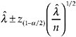
A (1 –α)100% confidence interval for the true suicide rate λ can be approximated as
(11)
where ![]() = y/n, y is the total number of suicides over n time intervals (e.g., months) or geographic areas (e.g. counties), and z is an upper percentage point of the normal distribution. In general, the approximation will work extremely well for y ≥ 20. When y < 20 tabled values are available in Hahn and Meeker (1991).
= y/n, y is the total number of suicides over n time intervals (e.g., months) or geographic areas (e.g. counties), and z is an upper percentage point of the normal distribution. In general, the approximation will work extremely well for y ≥ 20. When y < 20 tabled values are available in Hahn and Meeker (1991).
As an example, consider the case in which after 61 months of observation for a particular county, 123 suicides are recorded; therefore, y = 123 and n = 61. The 95% confidence limit for the population suicide rate λ is therefore
(12)
In light of this, we can have 95% confidence that the true suicide rate is between 1.659 and 2.373 suicides per month.
Poisson Prediction Limits
Cox and Hinkley (1974) consider the case in which y has a Poisson distribution with mean µ. Having observed y their goal is to predict y*, which has a Poisson distribution with mean cµ, where c is a known constant. In the present context, y is the number of suicides observed in n previous time-periods, and y* is the number of suicides observed in a single future time-period, therefore, c = 1/n. Alternatively, for a given time period, n may represent a number of counties, and our inference is to the predicted suicide rate in a single future county for the same length of time.
Following Cox and Hinkley (1974), Gibbons (1987) derived a prediction limit using as an approximation the fact that the left side of:
(13)
is approximately a standard normal deviate, therefore, the 100 (1 –a)% prediction limit for y* is formed from percentage points of the normal distribution. Upon solving for y* the upper limit value is found as the positive root of the quadratic equation:
(14)
Returning to the previous example in which after 61 months of observation for a particular county, 123 suicides are recorded, we have y = 123 and c = 1/61. The 95% confidence Poisson prediction limit is given by
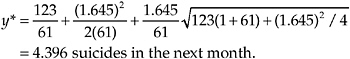
The prediction limit reveals that we can have 95% confidence that no more than four suicides will occur in the next month.
Poisson Tolerance Limits
The uniformly most accurate upper tolerance limit for the Poisson distribution is given by Zacks (1970). In terms of a future time interval, we can construct an upper tolerance limit for the Poisson distribution that will cover P(100)% of the population of future measurements with (1 – a)100% confidence. The derivation begins by obtaining the cumulative probability that a or more suicides will be observed in the next time period:
(15)
which can be approximated by:
Pr(a,μ) = Pr( χ2 [2a+2] ≥ 2μ
(16)
where χ2[f] designates a chi-square random variable with f degrees of freedom. This relationship between the Poisson and chi-square distribution was first described by Hartley and Pearson (1950). Given n independent and identically distributed Poisson random variables the sum
(17)
also has a Poisson distribution. Substituting Tn for μ, we can find the value for which the cumulative probability is 1 – α, that is,
(18)
The P(100)% upper tolerance limit is therefore Pr–1[P; K1–α(Tn)] = smallest j (≥ 0) such that
(19)
The required probability points of the chi-square distribution can be most easily obtained using the Peizer and Pratt approximation described by Maindonald (1984:294).
Returning to the previous example, where after 61 months of observation for a particular county, 123 suicides are recorded, we have, Tn = 123 and n = 61. Furthermore, we require the resulting tolerance limit to have 99% coverage and 95% confidence. The cumulative 95% probability point is
The 99% upper tolerance limit is obtained by finding the smallest nonnegative integer j such that:
Inspection of standard chi-square tables (extracted below for j = 5 to 7) reveals that the value of j that satisfies this equation is 7.
|
6 |
4.6604 |
|
7 |
5.8122 |
Therefore, the P–1 [.99 ; K.95(123)] upper tolerance limit is 7 suicides per month in the example posed.
REFERENCES
Beck AT, Steer RA. 1987. Beck Depression Inventory: Manual. San Antonio, TX: Psychological Corporation.
Bock RD, Aitkin M. 1981. Marginal maximum likelihood estimation of item parameters: an application of the EM algorithm. Psychometrika, 46: 443–459.
Böhning D, Schlattmann P, Lindsay BG. 1992. Computer-assisted analysis of mixtures (C.A.MAN): Statistical algorithms. Biometrics, 48: 283–303.
Böhning D, Dietz E, Schlattmann P. 1998. Recent developments in computer-assisted analysis of mixtures. Biometrics, 54: 525–536.
Böhning D. 1999. Computer-Assisted Analysis of Mixtures and Applications. Meta-Analysis, Disease Mapping and others. Chapman and Hall CRC: Boca Raton.
Cox C. 1995. Location-scale cumulative odds models for ordinal data: A generalized nonlinear model approach. Statistics in Medicine, 14: 1191–1203.
Cox DR, Hinkley DV. 1974. Theoretical Statistics. Chapman and Hall: London.
Dempster AP, Laird NM, Rubin DB. 1977. Maximum likelihood from incomplete data via the EM algorithm (with discussion). Journal of the Royal Statistical Society, Series B, 39: 1–38.
Gibbons RD. 1987. Statistical models for the analysis of volatile organic compounds in waste disposal sites. Ground Water, 25: 572–580.
Gibbons RD, Clark DC, Fawcet J. 1990. A statistical method for evaluating suicide clusters and implementing cluster surveillance. American Journal of Epidemiology, 132 (Suppl 1): S183–S191.
Hahn GJ, Meeker WQ. 1991. Statistical Intervals: A Guide for Practitioners. Wiley: New York.
Hartley HO, Pearson ES. 1950. Tables of the chi-squared integral and of the cumulative Poisson distribution. Biometrika, 37: 313–325.
Hedeker D, Gibbons RD. 1994. A random effects ordinal regression model for multilevel analysis. Biometrics, 50: 933–944.
Hedeker D, Mermelstein RJ. 1998. A multilevel thresholds of change model for analysis of stages of change data. Multivariate Behavioral Research, 33: 427–455.
Laird N. 1978. Nonparametric maximum likelihood estimation of a mixing distribution. Journal of the American Statistical Association, 73: 805–811.
Liang KY, Zeger SL. 1986. Longitudinal data analysis using generalized linear models. Biometrika, 73: 13–22.
Lindsay BG. 1983. The geometry of mixture likelihoods, part I: A general approach. Annals of Statistics, 11: 783–792.
Lindsay BG. 1995. Mixture Models: Theory, Geometry and Applications. NSF-CBMS Regional Conference Series in Probability and Statistics, Vol. 5. Hayward, CA: Institute of Mathematical Statistics.
Lindsay BG, Roeder K. 1992. Residual diagnostics for mixture models. Journal of the American Statistical Association, 87: 785–794.
Maindonald JH. 1984. Statistical Computation. Wiley: New York.
McCullagh P. 1980. Regression models for ordinal data (with discussion). Journal of the Royal Statistical Society, Series B, 42: 109–142.
McLachlan GJ, Krishnan T. 1997. The EM Algorithm and Extensions. New York: Wiley.
Miller IW, Norman WH, Bishop SB, Dow MG. 1986. The Modified Scale for Suicidal Ideation: Reliablity and validity. Journal of Consulting and Clinical Psychology, 54(5):724– 725.
Millon T. 1983. Millon Clinical Multiaxial Inventory Manual. 2nd ed. Minneapolis, MN: National Computer Systems.
Peterson B, Harrell FE. 1990. Partial proportional odds models for ordinal response variables. Applied Statistics, 39: 205–217.
Pilla RS. 1997. Improving the Rate of Convergence of EM in High-Dimensional Finite Mixtures. Ph.D. dissertation, The Pennsylvania State University.
Pilla RS, Lindsay BG. 2001. Alternative EM methods for nonparametric finite mixture models. Biometrika, 88: 535–550.
Rudd MD, Rajab MH, Orman DT, Joiner T, Stulman DA, Dixon W. 1996. Effectiveness of an outpatient problem-solving intervention targeting suicidal young adults: Preliminary results. Journal of Consulting and Clinical Psychology, 64(1):179–180.
Terza JV. 1985. Ordinal probit: A generalization. Communications in Statistical Theory and Methods, 14: 1–11.
Titterington DM, Smith AFM, Makov UE. 1985. Statistical Analysis of Finite Mixture Distributions. New York: Wiley.
Zacks S. 1970. Uniformly most accurate upper tolerance limits for monotone likelihood ratio families of discrete distributions. Journal of the American Statistical Association, 65: 307–316.
Zeger SL, Liang KY. 1986. Longintudinal data analysis for discrete and continuous outcomes. Biometrics, 42: 121–130.


