
4
Overview of Water Use Estimation
Though conceptually appealing, it is impossible to fully account in practice for all the individual decisions and behaviors that constitute the nation’s water use. Nevertheless, statistical sampling and indirect methods can be used to estimate aggregate water use. The diverse goals of water use estimation, and the varied categories and methods used to estimate water use, suggest no single approach can be—or should be—expected to satisfy all the requirements of the National Water-Use Information Program (NWUIP). The challenge of identifying an appropriate methodology—extensive data collection or indirect estimation—is evident in the National Handbook of Recommended Methods for Water Data Acquisition (USGS, 2000):
Water use can be determined either for site-specific facilities or for categories of water use for a given area. Determining site-specific water use involves water withdrawal, delivery, release, and return-flow data. Area estimates are based on coefficients relating water use to another characteristic, such as number of employees, and applying them to an inventory of site-specific users or by measuring a statistical sample of the user population.
Choosing whether to use site-specific data or area estimates to estimate water use will depend on the objective of the water use data collection; availability of statewide reported data; availability of time, manpower, and funds; and the area to be covered. The objective of the water use data collection determines the required degree of accuracy and reliability and identifies individual data elements that are relevant.
In contrast with data collection to compile a complete inventory of national water use, water use estimation requires statistical inference using inherently
mixed-quality data that are inconsistently sampled in time and space. Significant characteristics of water use estimation in the NWUIP include the following:
-
Estimates are necessarily grounded in local, individual data records. Estimates require integrating data of mixed quality that are collected by other agencies for other purposes and that are derived from data collection protocols generally neither controlled nor modifiable by NWUIP.
-
The water use database includes data on individual facilities that can be accurately tallied (such as public wells and permitted intakes), for which the associated water use is variable and uncertain and may be bounded (e.g., by a permit limit or water right).
-
The water use database includes data on diffuse uses that can be identified only through indirect measures (such as number of employees, dollar value of commercial manufacturing, cultivated acreage) and that can vary dramatically with climate variability and national economic trends.
-
Although grounded in local site-specific data, water use estimates must meet broader needs for information at state, regional, watershed, and national scales.
Historically, U.S. Geological Survey (USGS) national water use estimates have not been developed for a distinct client or constituency. Nor have they been developed in response to specific scientific or management goals. The result is a contextual void for evaluating the quality, accuracy, and value of the many data sources and estimation techniques used to populate this unique national database. The requirements for a water use estimation program suggested in this report underscore the need to quantify the accuracy and uncertainty of the national water use estimates.
A variety of methods will be required to populate a national water use database. The choice of estimation methods must balance the quality and availability of data, the information needs, and the available resources. The following section contrasts strengths and limitations of alternative methods for estimating water use.
DIRECT ESTIMATION
Direct estimation methods can be broadly divided into the complete inventory approach and the stratified random sampling approach. A complete inventory of water use seeks to quantify (by direct measurement or secondary records) every water use in a geopolitical or hydrologic region. The complete inventory is conceptually straightforward and has been the idealized model for the USGS water use program for several decades. It is also not possible or cost-effective in many cases, and sampling of a subset of the complete population is often the more reasonable approach.
Complete Inventory
A complete inventory presumes that all water uses can be identified and measured with sufficient resources and effort. Direct measurement reduces the water use estimation problem to a data collection and database management program. To support the conceptual model of a complete inventory of national water use, the USGS has wrestled with fundamental questions of defining water use and has developed a taxonomy of water use categories to support internally consistent accounting, comparison, and aggregation to regional and national scales. Without specific research goals or applications, the water use categories adopted to meet database challenges are intrinsically arbitrary. Indeed, the ambiguity in the purpose and goals of this data collection effort is evidenced by the evolution and redefinition of water use categories and data collections methods and even by the redefinition of water use in each of the Survey’s pentannual water use assessments. Nevertheless, the USGS water use categories provide an internally consistent data structure to formulate and organize water use estimates within each state.
The complete inventory model for national water use has pragmatic limitations. Consistent information collected at monthly, weekly, or daily time intervals would be difficult to compile. Useful ancillary data, such as the price of water, crop type, and soil characteristics, are not usually included in “inventory” datasets. In practice, a truly complete inventory of every national water use is unobtainable. Nevertheless, the diligent effort to scour every source and “all available” information naturally fosters the sense that these estimates must be the “best available,” regardless of the unquantified uncertainty in estimated use. Pragmatically, a complete inventory of all water uses is unachievable.
As a conceptual model, the USGS’s inventory of water use by category is little changed from water use estimation techniques used over 150 years ago (see Box 4.1). The closest example to a complete inventory in the USGS water use program may be the Arkansas water use program. Here, the coincidence of a newly established statewide water use permitting program adopting the USGS water use data management technology resulted in a unique partnership by which USGS provides both technology and database management for the entire permitting system. This cooperative partnership has provided the Arkansas District with one of the most complete and current water use databases in the country. It is important to note that the Arkansas water use database is defined by the state’s permit requirements and therefore emphasizes water use at the point of withdrawal. Water use information relevant for policymaking, such as domestic self-supplied water use, irrigation efficiency, the rate of industrial reuse, magnitude and location of return flows, and total stress on surface and groundwater, all require additional analysis and interpretation.
The complete inventory model is intuitively appealing and may be well suited to specific regulatory functions and permit needs. For example, river
|
BOX 4.1 The common use of a “complete inventory” of water-using activities, combining actual use with “water use coefficients” is neither novel nor unique to the USGS National Water Use Information Program (NWUIP). This intuitive “accounting” for water use is actually little changed (aside from the use of digital data management tools) from the methods used by the city of New York in estimating potential revenues for financing construction of the Croton Reservoir in the first half of the nineteenth century (Koeppel, 2000). “To determine the number of potential water users and how much they might be willing to pay, the commissioners drew a broad statistical portrait of 1835 New York. From information supplied by city surveyor Edwin Smith and others, the commissioners found that below its limits on 21st Street, New York contained 30,000 houses, over 2000 back tenements, 240 boarding houses, and 40 large hotels; 2,646 taverns and 100 victualing and refectory houses; 267 bakehouses, 63 distilleries, 12 breweries, 10 porter cellars, and 70 sugar houses; 178 printing offices, about 60 silversmiths and jewelers, 58 soap and candle factories, 43 marble and stone cutting works, and 10 type foundaries; 73 hatteries and 19 curriers and morocco manufacturers; 5000 horses, 237 butchers, 100 slaughter houses, 86 livery stables, and 1 tanyard; 26 classical schools, 23 primary schools, 22 female boarding schools, 12 public schools, and 7 ‘African free schools’; 60 steam engines (exclusive of those at distilleries, sugar houses, and stone works), 2 gas works, and 1 chemical factory. “Presuming that two-thirds of the houses and all other potential users would immediately sign up for Croton water, and after studying water use information solicited from other cities, the commissioners offer a table of estimated water revenue.” SOURCE: Koeppel (2000). |
basins that are highly regulated may require not only a complete inventory of withdrawals, but of return flows as well, in order to calculate consumptive use. At a larger scale, however, the principal limitation of the complete inventory model is the practical challenge of identifying and sampling every water use relevant for a national information program. When a complete inventory is impractical, water use may be estimated directly using formal sampling techniques, such as those described in Chapter 5.
Stratified Random Sampling
The enormous variation in both the quality of available water use data and the economic and climatic patterns of water use among the states poses substan-
tial challenges to any consistent national estimation framework. A rigorously formulated national sample design offers a practical means for developing consistent national water use estimates with uniformly quantified accuracy and reliability characteristics. One model for consistent national sample design is the Census of Agriculture of the USDA National Agricultural Statistics Service (NASS) (USDA, 1999a).
The Census of Agriculture uses a rigorous stratified sample design, employing both telephone and mail survey instruments, to develop detailed county-level estimates of national agricultural activities. Viewing the Census of Agriculture as a model for nationally consistent county-level stratified random sampling highlights a number of significant features and methodological issues that would be common to the national estimation of water use:
-
The sample design rigorously emphasizes computing the standard error, and hence confidence limits, on all estimates.
-
The program fosters an institutional culture of continuous improvement in sequential estimates. Each cycle of estimation draws upon lessons learned and observed trends from previous surveys, while simultaneously laying the foundation (through additional subsample survey questions) to evaluate emerging trends to be incorporated in future sample design.
-
Core expertise in sampling and research design is integrated with local and regional specialists throughout the states. This structure is suggestively similar to the infrastructure of the state water use specialists working with methodological guidance and statistical expertise found in the Water Resources Division of the USGS.
The culture of a continuously improving estimation process naturally leads to methodological research and evaluation of new techniques to improve accuracy and cost effectiveness. Such techniques include the following:
-
the use of screening models and follow-up surveys to evaluate the probability of membership in the sample population as part of the sampling design,
-
the use of remote sensing and expert systems for crop classification, mapping, and acreage estimation,
-
the use of follow-up evaluations to estimate the completeness of the target population coverage, evaluate nonresponse rates, and identify problems in order to improve future sample designs, and
-
of development techniques to extend survey estimates to nonsurvey years.
Stratified random sampling can optimally allocate limited sampling resources among homogeneous subpopulations, or strata, of a well-defined statistical population. Further, this sampling approach makes no assumptions regarding the probability distribution of the water use within a stratum (i.e., a normal distribu-
tion is not assumed). If reliable population data are available, accurate direct estimates of water use can be obtained with substantially less data collection than that required for complete inventory methods. However, this reduced sampling effort must be accompanied by the additional effort required to maintain current, accurate population information. If reliable population information is not available, their consistent water use estimates can be developed using indirect estimation methods.
INDIRECT ESTIMATION
Where direct sample data are inadequate or unavailable, indirect estimation methods may be used. Although indirect estimation methods can be extremely valuable when direct sample data are limited, these methods nevertheless require sufficient data to support calibration and verification. The following are required for indirect estimation: activity-based water requirements and water use coefficients, correlation-based models estimated with regression techniques, econometric models of water use behavior, materials flow models estimated from macroeconomic national accounts data, system-level models that explicitly optimize water use decision-making, and indirect methods for consumptive use.
Coefficient-Based Methods
Coefficient methods or unit use coefficient methods (including the well-known per capita methods) are widely utilized and are particularly well established in urban and municipal water use planning (Billings and Jones, 1996). Commonly used coefficient methods estimate water use as a constant requirement that scales linearly with a physical unit of activity, a dollar value of output, or the size of the water-using population. A more robust coefficient-based model calculates water use separately for specific categories (e.g., commercial, residential, industrial). When adequate categorical data are available, these estimates can be reaggregated to yield more accurate estimates of total water use.
Coefficient-based methods assume constant water use rates in each category of use. This simplification ignores trends, changes in water use due to conservation, technological change, or economic forces, and the optimal level of disaggregation of water use categories. The accuracy of coefficient-based estimates depends both on the water use coefficient and on the underlying activity assumed to drive water use (see Box 4.2). For example, in estimating future water use for the Washington, D.C., metropolitan area, Mullusky et al. (1995) used water use coefficients for three categories of water users: single-family homes, multiple-family homes, and employment water use. These categories were adopted not because of the a priori quality and accuracy of the water use coefficients, but because the underlying housing and employment data were uniformly and consistently available with high spatial resolution (Woodwell and Desjardin, 1995).
|
BOX 4.2 Coefficient methods estimate water use, W, as the product of a relevant explanatory variable X (number of employees, number of single-family homes, etc.) and a dimensionally consistent water use coefficient C (gallons per employee, gallons per single family home): W = XC. Coefficient or per capita water use estimation implicitly assumes all other explanatory variables either are irrelevant or are perfectly correlated with the single driving variable. A more robust estimation framework incorporates both X and C as random variables, with means μC and μX, standard deviations σC and σX, and correlation ρXC, making the water use estimate a function of these random variables whose properties can be explored. Considering the covariance of X and C (4.1) where the expected value of water use E[W] is given by (4.2) from which it is clear that the naive water use estimator E[W] = μXμC is biased unless X and C are uncorrelated. This simple treatment of uncertainty expands water use science in at least two ways. First, the explicit treatment of randomness in these planning-level estimators identifies a source of bias in the estimate and gives an analytical expression for that bias. Second, this simple analysis shows the importance of correlation between X and C, framing substantive questions for water science research and testable hypotheses that can be evaluated through well designed targeted data collection. For example, Equation 4.2 raises the significant question, “Is a nonzero correlation between X and C plausible?” Consider the simple coefficient estimate of employee water use in which X is the number of employees and C is the peremployee water use. Employee water use is commonly estimated with a water use coefficient, in part because employee data in one form or another are often readily available. It is easy to imagine C varying from establishment to establishment, so treating the water use coefficient as a random variable is fairly intuitive. The randomness in employment (or number of single-family homes, acres, etc.) |
The simple example in Box 4.2 shows how analyzing the properties and error characteristics of water use estimators can help structure hypothesis-driven water use science that can be tested in USGS district water use programs. This science improves our understanding of water use, with immediate returns in improved techniques for water use estimation and uncertainty analysis.
|
may be less intuitive because data such as data on employment often come from published sources as a single value. Nevertheless, recognizing the interpretation of X as a mean level of employment for the estimation period, any single value can only be an estimate of the constantly fluctuating employment base. Is it plausible for these two random variables to be correlated? Consider employment in a high-density office building. One can easily imagine a component of water use that is insensitive to employee numbers, such as water used for landscaping, evaporative cooling, cleaning, and building maintenance. Combining a relatively invariant water use with individual employee use varying linearly with employee numbers, one might reasonably postulate a negative correlation between X and C. This negative correlation immediately suggests a testable hypothesis that can be evaluated with a sound experimental design for data collection. Such applied water use science could be effectively coordinated among district water use programs throughout the country to stratify employee water use data by commercial density, climate zone, domestic product, etc. Indeed, the hypothesis-driven nature of the applied research strongly suggests the type of explanatory variables for which data should be collected in this experiment. The water science results would be expected to resolve the question of correlation between X and C, and to clarify some of the explanatory factors and climatic differences in these correlation patterns. These results would also feed directly back into the rule base for water use estimation as modified rules that now use Equation 4.2 as the improved water use estimator with the correlation, drawn from a database developed through targeted data collection, driven by hypothesis-based water use science. Finally, having resolved this meaningful question of correlation, confidence limits on the coefficient-based estimate can also be computed. Schwartz and Naiman (1999) showed that a distribution free estimate of the standard deviation of equation 4.2 is given by: (4.3) With the stronger assumption that the joint distribution of X and C are lognormal, the standard deviation of the water use estimate is given by: (4.4) where νx and νc are the coefficients of variation of X and C, respectively. |
Multivariate Regression
Multivariate regression methods, such as those described in Chapter 6, systematically utilize the correlation structure of observed water use and explanatory variables under the familiar assumptions of the standard linear model. For example, the regression of crop yields on evapotranspiration is widely used in
irrigation planning (Nielsen, 1995). In general, multivariate regression models are variations of “water requirement” models in which water use is computed at a fixed, activity-specific rate that is estimated statistically from observed data. For example, most of the observed variability in municipal water use can be explained by exogenous variables representing population and meteorology. Ancillary explanatory variables such as disaggregated data on housing price, per capita income, lot size, and water rates can further explain the variance in observed water use, when such data are available. Of course, explanatory variables such as property value do not directly cause water use. Rather, explanatory variables serve as readily available covariates of water-using activities that tend to be strongly correlated with the readily available data such as data on property value.
The most significant issues in modeling water use with multivariate regression are typically (1) selection of the “best” set of explanatory variables, (2) the form of the regression equation, and (3) parameter estimation. The choice of explanatory variables artfully balances plausible causal factors with the observed correlation structure of available data. The well-known challenges of distinguishing correlation and causality particularly apply to water use. Price sensitivity, technological innovation, and scarcity can result in significant changes over time that may easily be misinterpreted as a trend because of their gradual effect and consequent correlation with time. For example, the dramatic increases in manufacturing and industrial water use efficiency over the last 30 years are well documented (see Table 4.1). This “trend” is largely explained as the response to wastewater treatment costs associated with passage of the Clean Water Act in 1972. This historical change in industrial water use would be correlated with a variable representing time. However, a regression model using time as an explanatory variable unrealistically assumes that the dramatic reductions in water use that have resulted from technological process changes and recycling will continue in the future at the same rate.
Similarly, the form of the regression equation should reflect the structural relationship between water use and explanatory variables—not just their linear
TABLE 4.1 Recycling Rates for Various Industries in the U.S.
|
Industry |
1954 |
2000 |
|
Paper |
2.4 |
11.8 |
|
Chemicals |
1.6 |
28.0 |
|
Petroleum |
3.3 |
32.7 |
|
Primary Metals |
1.3 |
12.3 |
|
Manufacturing |
1.8 |
17.1 |
|
SOURCE: Thompson (1999). |
||
correlation. Municipal water use typically correlates to seasonal changes in temperature and precipitation. Hot, dry weather tends to increase water use. However, in comparing municipal water use in Northern Virginia and Los Angeles, Whitcomb (1988) found that the climatic differences between the two systems required fundamentally different water use models. In temperate Northern Virginia, it is uncommon to have more than five consecutive summer days without measurable precipitation. The most parsimonious model for Northern Virginia water use explained increases above the mean seasonal water use by the number of consecutive antecedent dry days. In contrast, during the dry season in Los Angeles, mean seasonal water use is insensitive to the number of antecedent dry days, but unusually cool or wet weather can decrease municipal water use from the seasonal mean. Although meteorological anomalies are generally correlated with water use, model specification for multivariate and time series models must be carefully matched to system characteristics.
Finally, the complex correlation structure of water use and candidate explanatory variables almost always violates the assumptions of the standard linear model, motivating substantial research on alternatives to ordinary least squares for parameter estimation. This becomes necessary when the most highly correlated explanatory variables are themselves both correlated to, and functions of, water use. For example, the Massachusetts Water Authority (MWA) undertook an aggressive conservation program when water use grew to exceed the yield of Quabbin Reservoir. Water use was successfully reduced through a combination of industrial process changes in the metal plating industry, correction of a leak detected in a distribution system with vintage water mains, and residential water audits. The intensity of MWA’s water conservation program (quantifiable by measures such as the annual program budget or the number of water-conserving devices installed) will be correlated with reductions in water use. The intensity of the conservation program will also be a function of water use—with greater water use eliciting greater investment in conservation. The effect of the residential conservation program is further confounded by the fact that water rates dramatically increased at the same time (to finance massive infrastructure investment in wastewater treatment) and are therefore correlated with conservation investment. This complexity, typical in water use estimation, suggests the need to model water use as more than just a material requirement correlated with activity indicators. Water-using behavior is the result of consumer choices and policy interventions that can be understood using econometric methods.
Econometric Methods
Econometric methods also estimate water demand using regression-based techniques. However, an econometric approach to water use estimation implies more than including economic explanatory variables in multivariate regression. An econometric approach to water use estimation starts from the fundamental
premise that the demand function for water is the solution to consumers’ constrained optimization problems and therefore varies with the price both of water and all other goods and services. The economic demand function represents water-consuming behavior. In contrast, water requirement or empirical regression models implicitly treat water as a fixed technical requirement.
The contrast between regression and econometric approaches to water use estimation can be highlighted by considering the choice of explanatory variables used to estimate municipal water use. A typical model of municipal water use might include variables representing population, weather, lot size, household income, and binary “dummy variables” indicating the presence or absence of swimming pools and water-conserving fixtures (Billings and Jones, 1996). A variable such as the price of electricity would be unlikely to appear in such a model. In contrast, the cost of electricity might be a natural variable to include in an econometric model of water use, because water and electricity are both critical inputs to household activities, and their relative prices influence consumption decisions. For example, the peak supply problems affecting the electrical grid in California in 2001 have led to calls for consumers to conserve electricity by only running dishwashers and washing machines with full loads. Such a behavioral change could be expected to result in a marginal decrease in water use. This decrease would be expected not because of collateral stimulation of consumers’ conservation ethic, but rather because water and electricity are complementary inputs to the production of dishwashing and laundry services. Their joint consumption is defined by the “production function” for these activities.
Water and electricity may also be substitutes in providing cooling and air conditioning services. Residential evaporative cooling—commonly used, for example, in the city of Phoenix—requires only a third to a fifth the electricity of air conditioning. This reduced power consumption is associated with substantial—and highly variable—water use requirements, variously estimated between 95 and 200 gallons per day (Karpisack and Marion, 1994). Indeed, the adoption of evaporative cooling (with its associated increase in water use) was promoted as a means of reducing electricity consumption following escalating energy costs in the 1970s. Water is a direct substitute for energy in this application. However, Karpisack and Marion (1994) point out that, indirectly, water and electricity are complementary inputs, because water is used to produce electricity, and electricity is required to treat, pump, and deliver water.
The economic demand function for water may also be derived as the solution to an optimization problem that explicitly incorporates the underlying water-consuming technological choices and economic objectives driving water use decisions (Gisser, 1970). Such explicit optimization approaches have been extensively used in analyzing water use in California’s Central Valley. For example, Howitt et al. (1999) used the Statewide Water Agricultural Production model (SWAP) to quantify the potential gains from exploiting the spatial and temporal differences in the marginal valuation of water. They did this by assess-
ing agricultural users’ willingness to pay for reliable water supply. For 25 regional production areas (including the 21 regions of the Central Valley Production Model plus southern California), water application is determined from the solution of regional constrained optimization problems that allocate land, water, and capital to equate the marginal product and marginal cost of water use (Howitt et al., 1999). The total amount of irrigated land in production varies with both the price and availability of water, reflecting the marginal expansion and contraction of irrigated acres as junior water rights are fulfilled.
National Accounts And Input-Output Modeling
The role of water as a commodity and economic input can be quantified through the system of national industrial accounts maintained by the Bureau of Economic Analysis (BEA). BEA consistently quantifies economic flows appearing as market transactions in the national economy at the county, regional, and national levels (Figure 4.1).
Economic activity is quantified as the dollar value of goods and services supplied to industries and final consumers, disaggregated by Standard Industrial Classification (SIC) Codes—or by the North American Industry Classification System (NAICS). One potential use of this uniformly available data is the estimation of water use through the direct use of economic flows reported from the different industrial uses corresponding to the water industry. SIC codes 4941 and 4971 include water supply and irrigation services, respectively. Clearly, the dollar value of market transactions from these industrial sectors reflects total economic output, not just water use. Moreover, significant nonmarket water uses (such as self-supplied wells and instream flows) are not well documented in these national reports. Nevertheless, it may be possible to derive water use coefficients that apply specifically to SIC codes, having units of gallons per dollar. As with all coefficient methods, the quality of the estimate will depend on the quality of both the derived water use coefficient and the estimated magnitude of the underlying activity (i.e., sales). In this case, the consistent availability of economic activity data by sector may warrant the effort to develop appropriate water use coefficients to exploit this high-quality data source.
The BEA also maintains secondary data that track the changes in economic activity throughout the nation. This activity data may be very useful as direct “explanatory variables” for water use estimation. Of perhaps greater value is the potential use of these data to identify significant structural changes and trends in regional economic activity that will require additional scrutiny and investigation to accurately update regional water use estimates. As a consistent indicator of county-level economic activity, BEA’s regional economic data may be an efficient starting point in the sampling and design of each cycle of national water use estimation. An example in Table 4.2 shows data on county-level employment, which is uniformly available as part of the BEA Regional Accounts Data. These
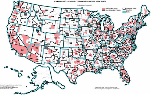
TABLE 4.2 Full-time and Part-time Employment (Number of Jobs) by Industry, Montgomery County, Maryland, 1994–1998
|
|
Number of Jobs |
||||
|
Industry |
1994 |
1995 |
1996 |
1997 |
1998 |
|
Total |
509,120 |
526,404 |
532,652 |
548,047 |
566,575 |
|
Farm |
881 |
876 |
844 |
873 |
784 |
|
Non-Farm |
508,239 |
525,528 |
531,808 |
547,174 |
565,791 |
|
Private (non-farm) |
421,000 |
436,579 |
445,955 |
462,399 |
480,756 |
|
Agriculture |
5,480 |
5,494 |
5,623 |
5,678 |
5,773 |
|
Mining |
605 |
646 |
520 |
566 |
558 |
|
Construction |
28,672 |
28,823 |
28,811 |
29,905 |
30,197 |
|
Manufacturing |
17,947 |
17,700 |
18,549 |
20,131 |
20,428 |
|
Transportation and Public Utility |
15,449 |
15,731 |
14,716 |
14,845 |
16,897 |
|
Wholesale Trade |
15,521 |
16,122 |
15,711 |
15,513 |
15,417 |
|
Retail Trade |
76,421 |
77,764 |
78,454 |
80,777 |
81,640 |
|
Finance, Insurance, Real Estate |
52,269 |
55,899 |
56,776 |
58,474 |
60,688 |
|
Services |
208,636 |
218,400 |
226,195 |
236,510 |
248,558 |
|
Government and Government Enterprises |
87,239 |
88,949 |
86,453 |
84,775 |
85,635 |
|
Federal, civilian |
44,069 |
44,682 |
43,021 |
41,517 |
41,289 |
|
Military |
8,161 |
8,111 |
7,834 |
7,404 |
7,242 |
|
State and Local |
35,009 |
36,156 |
35,598 |
35,854 |
37,104 |
|
State |
1,673 |
1,664 |
1,442 |
1,202 |
1,239 |
|
Local |
33,336 |
34,492 |
34,156 |
34,652 |
35,865 |
|
SOURCE: BEA Regional Accounts Data (http://www.bea.doc.gov/bea/regional/reis/action.cfm). |
|||||
data would naturally support a simple coefficient-based water use estimation model for “employee water use.” The consistent national availability of these county-level data may well justify the effort to refine employee water use coefficient estimates. For example, the pattern and structure of “employee water use” coefficients among the states could be systematically investigated through a series of state-level studies coordinated through the NWUIP, accounting for regional differences in climate and economic trends. The result of these investigations would feed back to the water use program in the form of improved procedures and quantitative uncertainty analysis for national estimation of employee water use with coefficient methods.
INPUT–OUTPUT TABLES AND MATERIALS FLOW ANALYSIS
A disaggregated static “snapshot” of the flows of goods and services in the market economy is also reliably available in national Input-Output (I-O) tables.
I-O tables consist of a matrix showing the interindustry purchases and final sales to users and the commodity inputs required by an industry to produce its output. Detailed I-O tables for the United States are available at several levels of disaggregation, with the most detailed accounting for 490 industrial sectors. At the level of so-called “two-digit” industrial codes, the I-O tables aggregate to 97 distinct industrial sectors. Market transactions related to water use are captured in I-O Industry Code 68C: Water and Sanitary Services.
I-O modeling can capture both direct and induced water uses associated with a unit of production. In this way, I-O analysis allows the total water use inputs to be quantified for a unit of output from every industrial type. For example, water is used directly in manufacturing an automobile (e.g., as both process water and for cooling, drinking, and sanitary services within the plant). Automobile production also uses water indirectly, in the steel, fabric, and other intermediate material inputs to the manufacturing process. Table 4.3 illustrates estimates of embodied water content for various commodities. The I-O table can be used to compute the total (direct and indirect) output required from every industry to produce the disaggregated gross national product of the United States. The I-O tables also represent a set of linear production functions (constraints) for the national economy (under the static assumption of constant technology).
The economic flows quantified in the national I-O tables can also be used to estimate material flows in the economy. Figure 4.2 represents the approach described by Biviano et al. (1999) for estimating the material flows of lead. The methodology draws upon similar efforts by the Department of Defense to estimate strategic material requirements and by the U.S. Bureau of Mines (efforts now conducted by the USGS Minerals Information Team). Similar materials flow analyses have been developed for metals and minerals ranging from arsenic cadmium salt and lead to mercury, zinc, and crushed aggregate for concrete. The approach combines National Accounts Data from I-O tables with available materials requirements by industry. The result integrates industry requirements and macroeconomic feedbacks to estimate the total material flow embodied in the final production of each sector of the economy.
TABLE 4.3 Embodied Water Use for Producing Various Products
|
Product |
Water Use (gallons) |
|
Automobile (1) |
100,000 |
|
Cotton, 1 lb. |
2,000 |
|
Aluminum, 1 lb. |
1,000 |
|
Corn, 1 lb. |
170 |
|
Steel, 1 lb. |
25 |
|
SOURCE: Thompson (1999). |
|
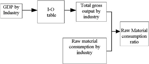
FIGURE 4.2 General methodology for estimating materials flows. GDP is gross domestic product. SOURCE: Biviano et al. (1999).
Although materials flow analysis has primarily focused on minerals, metals, and energy, the combination of BEA economic accounts data and the USGS water use estimates suggests an analogous approach to describing the flow of water through the economy. In the growing field of materials flow analysis and industrial ecology, Wernik and Ausebel (1995) observe that, on a mass basis, the material flow for water is more than 25 times greater than any other material flow in the economy.
Augmented Income and Product Accounts
The existing system of National Income and Product Accounts, along with National Accounts Data and Regional Accounts Data maintained by the BEA, can be an extremely useful source of nationally consistent, county-level data on industry-disaggregated economic activity. The convention that counts only market transactions yields an incomplete representation of national economic activity. For example, cutting both commercially managed and first-growth forests represents drawdowns of national wealth, yet only the former asset loss is recorded in the national accounts. Recognizing the distortions introduced by these conventions, the BEA has begun to develop satellite or “augmented economic accounts” with the goal of accounting for as much economic activity as is feasible, regardless of whether it takes place inside or outside the marketplace (NRC, 1999).
In reviewing the initial and proposed augmentation of the national accounts, the NRC Panel on Integrated Environmental and Economic Accounting found the development of environmental and natural resource accounts to be an essential investment for the nation. The panel concluded that the development of appropri-
ate accounts for the water resources sector should be a high priority. The panel also found that to improve environmental accounting, one must improve the physical measures of stocks and flows on natural resource assets, noting that generally “… there are no routine measures when these flows take place outside of the marketplace” (NRC, 1999). The structure of the USGS water use estimates is particularly well suited to supporting the national accounting for the “near-market” water use services that permeate the economy. Indeed, the USGS water use program was identified as the only source of physical data on water use cited by the panel (NRC, 1999). The panel concluded:
Much of the information needed to construct and maintain environmental accounts would be highly useful to other federal agencies, particularly for natural assets under federal stewardship and for environmental activities for which the federal government has responsibility to undertake benefit-cost analysis. A cooperative and coordinated approach among analytic teams of researchers from different federal agencies and the private sector to collect, analyze, and manage improved natural-resource and environmental data would be valuable not only for developing natural resource and environmental accounts, but also for promoting better monitoring, assessment, and policy making in these areas.
The consistently high-quality data in BEA’s national and regional accounts have great potential to serve as a valuable source of consistent data for both screening, trend identification, and water use estimation. As well, the USGS water use program is a unique source of national data on the nonmarket activities derived from the nation’s water resources as they flow through both the economy and the hydrologic system. There is great potential for cooperation and coordination between the NWUIP and the BEA, galvanized by the mutual interest in “promoting better monitoring, assessment, and policy making” for the nation.
Indirect Estimates of Consumptive Use
Consumptive use is nearly impossible to measure directly on any scale except the experimental scale. Thus, indirect methods are almost always used.
The simplest method, and a commonly used one, is to estimate consumptive use as the residual of other metered or estimated quantities. For example, consumptive use may be estimated as withdrawals minus return flow for a public-supply system. In this case, consumptive use includes such disparate processes as evaporation from reservoirs or canals, leakage from pipes, public use (street cleaning, fire fighting), theft, etc. A similar calculation could be made for irrigation systems, if conveyance losses can be estimated.
Simple coefficient methods are also commonly used. For example, domestic self-supplied consumptive water use (lawn watering, cooking, etc.) is typically estimated as a percentage of water withdrawn. The withdrawals themselves are typically estimated using per capita coefficients that vary by location. A similar methodology may be used for industrial consumptive use, based on SIC code.
These estimates are highly subject to error depending on the age and specific type of the facility.
Physically based estimates are commonly used for irrigation consumptive use. This is a broad and important topic that cannot be treated in detail here; the reader is referred to Allen et al. (1996) and Jensen et al. (1990) for extensive discussions on the subject. Some of the common methods use empirical correlations between evapotranspiration and climatic factors; others use energy- or water-budget approaches. In the last decade, efforts have been under way to construct spatially integrated fluxes of water by combining eddy flux measurements with satellite measurements and various models. Information on FLUXNET, a global network of such micrometeorological sites, is available at http://www.daac.ornl.gov/FLUXNET/fluxnet.html.
Finally, several of these methods may be combined with remote sensing techniques. For example, The Lower Colorado River Accounting System (LCRAS) estimates and distributes consumptive use by vegetation to water users along a sector of the river, as required by the U.S. Supreme Court decree, 1964, Arizona v. California. LCRAS uses a water-budget method to estimate annual consumptive use by vegetation. Then it combines this output with that from digital-image analysis of satellite images, estimated water use rates by vegetation types, and digitized boundaries for diverters (Owen-Joyce and Raymond, 1996).
CONCLUSIONS AND RECOMMENDATIONS
Compiling a complete inventory of all water use in the United States is intuitively appealing, but impractical. This chapter provides an overview of the diverse methods available to estimate water use when direct measurements and observations are unavailable. All of these methods address both the quantitative estimation of water use and the uncertainty of the estimate. No single approach to water use estimation can be expected to satisfy all the requirements for the NWUIP. Nevertheless, rigorous estimation of water use, matching appropriate methods to available data and objectives, should be a fundamental component of the NWUIP.
The committee therefore recommends that the USGS undertake a systematic national comparison of water use estimation methods in order to identify the techniques that are best matched to the requirements and limitations of the NWUIP. The USGS’s structure of state water use specialists and statistical expertise in the National Research Program is ideally suited to this undertaking.
The power of statistical sampling and estimation to rigorously address uncertainty, and to identify and exploit the inherent structure in water use, is illustrated in detail in Chapters 5 and 6.


