
2
Sources of Sound in the Ocean and Long-Term Trends in Ocean Noise
INTRODUCTION
In this chapter the major natural (physical and biological) and anthropogenic contributors to ocean noise are discussed. Gaps in our knowledge or available data are identified that will need to be addressed in future research in order to develop predictive models of the effects of noise on marine mammals. A more thorough description of modeling efforts is contained in Chapter 4.
This chapter focuses on the properties of the sources and does not describe in detail the effects on the environment as the acoustic energy travels away from the vicinity of the sources. Parameters such as source level (in units of dB re 1 µPa at 1 m), source spectral density level (units of dB re 1 µPa2 per Hz at 1 m), and time-integrated source pressure amplitude squared for use with transient signals (units of dB re 1 µPa2 at 1 m) are presented for many of these sources, particularly man-made sources. However, accurate estimation of the source properties for many types of naturally occurring sounds is impossible, given the lack of knowledge of the individual source locations, of the spatial distribution of multiple contributing sources, and of the complex propagation conditions. Therefore, in such situations, the measured properties of the received acoustic field (which are obtained directly and require no additional information, computation, or assumptions, but which contain the effects of propagation) will be presented. The text clearly differentiates between the properties of the sources and those of the received field. The distinction between source level and received level also is discussed both in Chapter 1 and in the Glossary.
In the absence of shipping, natural forces are the dominant sources of the long-term time-averaged ocean noise at all frequencies. In the presence of distant shipping, contributions from natural sources continue to dominate time-averaged ocean noise spectra below 5 Hz and from a few hundred hertz to 200 kHz. The dominant source of naturally occurring noise across the frequencies from 1 Hz to 100 kHz is associated with ocean surface waves generated by the wind acting on the sea surface. Nonlinear interactions between ocean surface waves called microseisms (see the Glossary; referred to as “Surface Waves—Second-Order Pressure Effects” in Plates 1 and 2) are the dominant contributors below 5 Hz, while thermal noise (i.e., the pressure fluctuations associated with the thermal agitation of the ocean medium itself) is the dominant contributor above 100 kHz. Natural biological sound sources make a noticeable contribution at certain times of year. For example, a peak around 20 Hz created by calls of large baleen whales is often present in deep-ocean noise spectra. Groups of whistling and echolocating dolphins can raise the local noise level at the frequencies of their signals. Snapping shrimp are an important component of natural noise from a few kilohertz to above 100 kHz close to reefs and in rocky bottom regions in warm shallow waters. Fish can add to ocean noise in some locales.
Whether intentional or unintentional, anthropogenic noise in the marine environment is an important component of ocean noise. Sound is a widely used tool for a broad range of marine activities. In the search for new hydrocarbon reserves, the rock underlying the seafloor is characterized using air-guns. Marine researchers use sound waves to investigate the properties of seawater both for local and global studies. Sonars used for civilian navigation and defense purposes use sound waves to locate objects under the sea surface. Unintentional contributions to marine noise arise from transiting ships, coastal and marine construction activity, mineral extraction, and aircraft overflights. These anthropogenic sound sources contribute to ocean noise over the complete 1-Hz to 200-kHz band of interest in this report. In the lowest bands, 1-10 Hz, the contributors are ship propellers, explosives, seismic sources, and aircraft sonic booms. In the 10-100 Hz band, shipping, explosives, seismic surveying sources, aircraft sonic booms, construction and industrial activities, and naval surveillance sonars are the major contributors. For the 100-1,000 Hz band, all the sources noted for the 10-100 Hz band still contribute. Also, the noise from nearby ships and seismic air-guns can extend up into the 1,000-10,000 Hz band. This band also includes underwater communication, naval tactical sonars, seafloor profilers, and depth sounders. The 10,000-100,000 Hz band includes the systems listed, in addition to mine-hunting sonars, fish finders, and some oceanographic systems (e.g., acoustic Doppler current profilers). Anthropogenic contributors at and above 100,000 Hz are limited to mine hunting, fish finders, high-resolution seafloor mapping devices
such as side-scan sonars, some depth sounders, some oceanographic sonars, and research sonars for small-scale oceanic features (Table 2-1a and 2-1b).
Prior to considering anthropogenic sources, it is useful to first understand the natural sources that contribute to ocean noise. Presumably, hearing and communication systems of marine organisms are adapted to these natural noises.
NATURAL SOURCES OF OCEAN NOISE
Physical and Geophysical Sources
The ocean is intimately coupled to the solid earth and the atmosphere, and in fact, most of the significant physical sources of natural sound occur at the interfaces among these three media. Additional sound in the marine environment originates in the atmosphere and penetrates the ocean surface. Elastic vibrations in the earth also introduce sound into the underwater acoustic field.
Sources at the Ocean Surface
The dominant physical mechanisms of naturally occurring sound in the ocean occur at or near the ocean surface. Most are associated with wind fields acting on the surface and the resulting surface wave activity. In the absence of man-made, biological, and transient sounds, ambient noise is wind dependent over the band from below 1 Hz to at least 50 kHz. Below 5-10 Hz, the dominant ambient noise source is the nonlinear interaction of oppositely propagating ocean surface waves. These sounds are called microseisms. (The term “microseisms” comes from the fact that they also are the dominant source of noise in high-quality, on-land seismometer measurements; however, the source mechanism for microseisms is unrelated to seismic processes in the solid earth.) Across most of the remainder of this band, the primary sources are bubbles that are oscillating, both individually and collectively in a cloud, in the water column. Several good references on natural physical sources of ocean noise and the properties of the ambient noise field are available (e.g., Urick, 1984; Zakarauskas, 1986; Ross, 1976; Kerman, 1988, 1993; Buckingham and Potter, 1995; Leighton, 1997; Deane, 1999). Only a brief summary of the major contributors to the underwater sound field is given here. However, in some frequency bands such as the band from 10 to 200 Hz, where ambient noise in the northern hemisphere typically is dominated by shipping noise, the dominant source mechanisms have not been identified. Quantification of the relative contributions of the various mechanisms of naturally occurring sound created at the sea surface remains an active area of research.
The average ocean noise spectrum can be empirically described and
TABLE 2-1a Characteristics of Anthropogenic Contributors to Marine Noise
|
SOURCE |
SPATIAL VARIABILITY |
DIRECTIONALITY |
ACTIVITY LEVELS |
|||
|
|
Large Scale Ocean Basin to Global |
Mid Scale 10s of km to Ocean Basin |
Small Scale <1 km to 10s of km |
|
Number of Regional Sources |
Frequency of Activity in Region |
|
Shipping |
Presence is global for all types and limited to the ocean surface |
|
||||
|
Merchant |
Shipping lanes transcend ocean basins and are populated continuously |
|
1-2 |
4-5/hr |
||
|
Utility |
|
Operations are confined to subocean basins and localized areas such as fishing grounds |
|
1-30 |
daily |
|
|
|
|
|
All shipping: Generally considerd to be omnidirectional, but shielding is certainly present in the horizontal plane, especially for the higher frequencies; omnidirectional in the vertical plane. |
|
||
|
Military |
|
Operations are military exercises, war zones |
Extending down to amphibious assault zones, beach heads |
|
6-10 |
bi-monthly |
|
Scientific |
|
Specific sites to observe phenomena of limited spatial scales |
Down to localized phenomena such as “black smokers” |
|
1-2 |
monthly |
|
Recreation |
|
|
Coastal regions, limited range |
|
>10 |
>5/day |
|
Other |
E.g., transoceanic cable laying |
Localized operations |
E.g., drill site |
|
|
>monthly |
|
Seismic exploration |
|
Surveys to >100 km |
Down to 10s of km |
Omnidirectional |
1 |
monthly |
|
Sonars |
Global presence, but variability is defined by sonar use |
|
||||
|
Military |
|
|||||
|
Surveillance |
Ocean basin use |
Down to 10s of km |
|
Omnidirectional |
1 |
monthly |
|
Tactical |
|
10s of km and up, conditions permitting |
|
Horizontal plane, Vertical >100°, Vertical plane <20° |
2-3 |
See host platform data above |
|
Weapon/ Counter Weapon |
|
10 m to >10 km |
Highly directional in both planes (<5°) |
1-2 |
|
|
|
Civilian |
|
|||||
|
Communications |
|
10s of km and up |
Down to >1 km |
Horizontal plane: omni Vertical plane: <10° |
1 |
|
|
SOURCE |
SPATIAL VARIABILITY |
|
DIRECTIONALITY |
ACTIVITY LEVELS |
||
|
|
Large Scale Ocean Basin to Global |
Mid Scale 10s of km to Ocean Basin |
Small Scale <1 km to 10s of km |
|
Number of Regional Sources |
Frequency of Activity in Region |
|
Navigation |
|
<1 km to <10 km |
Omnidirectional |
1 |
|
|
|
Hi-resolution |
|
>10 m to >100 m |
Highly directional (almost all look down or up) |
1-2 |
|
|
|
Marine Research |
Limited ocean basin tests |
Spatial interest to ocean basin dimensions |
Down to sub-meter measurements |
See sonars / military and civilian |
1 |
monthly |
|
Explosions |
|
<1 km |
Omnidirectional |
1 |
seldom |
|
|
Industrial Activity |
Presence is global and limited to near-shore locations/onshore locations |
|
||||
|
Construction |
|
<1 km to 10s of km |
Omnidirectional |
1 |
|
|
|
Dredging |
<1 km to 10s of km |
Omnidirectional |
1 |
|||
|
Power plants |
100s of m |
Omnidirectional |
1 |
|||
|
Factories |
100s of m |
Omnidirectional |
1 |
|||
TABLE 2-1b Characteristics of Anthropogenic Contributors to Marine Noise
|
SOURCE |
TEMPORAL VARIABILITY |
|
SOURCE CHARACTERISTICS |
|
||
|
|
Large Scale wks to mos |
Mid Scale hrs to days |
Small Scale sec(s) to min(s) |
Signal Structure |
Spectral Content |
Source level dB re 1µPa at 1 m |
|
Shipping |
|
See Figure 2-1 for example |
|
|||
|
Merchant |
Constant presence |
|
occasional transient due to operations activity on vessel |
|
160–220 |
|
|
Utility |
On site for wks |
Down to hrs |
|
numerous transients due to nature of operations |
For all shipping, broadband energy from 10 Hz to >1 kHz with spectral lines rising above B/B due to propulsion blades, turbines, generators, etc. |
160−200 |
|
|
Transient additions are broadband and flat from 10 Hz to 1 kHz |
160−200 |
||||
|
Military |
|
On site for hrs to days |
|
general level up and down with exercise/war fighting requirements |
|
160–220 |
|
Scientific |
On site for days |
Down to min(s) |
stop and start behavior driven by data collection schedule |
160–200 |
||
|
Recreation Other |
Wks |
Typically hrs days /hrs |
Or less |
highly variable |
160–190 |
|
|
Seismic exploration |
|
On site for days |
|
Impulsive (see Figure 2-4) |
Broadband |
>240 |
|
Sonars |
|
|||||
|
Military |
|
|||||
|
Surveillance |
On site for wks |
Down to days |
|
Pulsed tones |
<1 kHz |
>230 |
|
Tactical |
|
On site for hrs |
Down to min(s) |
Pulsed tones |
>1 kHz to <10 kHz |
200 to 230 |
|
Weapon/ Counter Weapon |
hrs to ~ a day |
Down to min(s) |
Pulsed tones / Wideband pulses |
>0 kHz to >100 kHz |
190 to 220 |
|
|
SOURCE |
TEMPORAL VARIABILITY |
|
SOURCE CHARACTERISTICS |
|
||
|
|
Large Scale wks to mos |
Mid Scale hrs to days |
Small Scale sec(s) to min(s) |
Signal Structure |
Spectral Content |
Source Level dB re 1 µPa at 1 m |
|
Civilian |
|
|||||
|
Communications |
|
hrs |
To min(s) tones |
CW/Pulsed |
Low kHz to >10 kHz |
180-210 |
|
Navigation |
|
hrs/days |
min(s) |
CW/Pulsed |
Low kHz to >10 kHz |
180-210 |
|
Hi-resolution |
|
min(s) |
Pulsed tones |
>10 kHz to >100 kHz |
160-220 |
|
|
Acoustic |
|
Series of pulses 10-500 msec w/ interpulse periods of 0-10 sec |
5-30 kHz typically |
130-150 |
||
|
Harassment or Deterrent Devices (AHD, ADD) |
|
|||||
|
Marine Research |
|
Down to days/hrs |
|
See military/civilian sonars |
See military/ civilian sonars |
160–220 |
|
Explosions |
|
sec(s) |
Impulsive (see figure) |
Broadband |
>240 |
|
parameterized according to sea state (Knudsen et al., 1948). These Knudsen curves are straight lines of spectral density as a function of frequency when plotted on a logarithmic scale. The parallel nature of the “curves” for various sea states signifies that the noise level increases with increasing sea state by the same amount at all frequencies. Although developed more than a half-century ago, the Knudsen curves continue to be widely used to predict natural ocean noise levels at frequencies from 1 to 100 kHz. The pioneering Knudsen’s curves of noise as a function of sea state have been very useful for many years and are remarkably effective, but it is now well established that the noise is correlated much better with wind speed than with sea state or wave height (correlation of wind speed and sea state only occurs in equilibrium conditions). This correlation with wind speed allows much more effective prediction and forecast (from wind forecasts) than could be obtained from sea state, which is difficult to estimate reliably.
Although open-ocean breaking wave noise is correlated with wind speed, local winds are not required to create the sounds from breaking surf. The sound created by spilling breakers (breaking begins at the wave crest and proceeds down the face of the wave) is primarily at the higher frequencies, whereas that from plunging breakers (the water at the wave crest leaps ahead of the wave in a jet, encompassing a large column of air) is significantly greater in levels and in frequency bandwidth. Plunging surf can raise underwater noise levels by more than 20 dB a few hundred meters outside the surf zone across the band from 10 Hz to 10 kHz (Wilson et al., 1985).
Precipitation on the ocean surface also contributes sound to the ocean. Rain can increase the naturally occurring ambient noise levels by up to 35 dB across a broad range of frequencies extending from several hundred hertz to greater than 20 kHz. For drizzle in light winds, a broad spectral peak 10-20 dB above the background occurs near 15 kHz (Nystuen and Farmer, 1987; measurements made at 7.5 m depth in an 8 m deep spot in a soft-bottom lake, Nystuen, 1986).
Atmospheric Sources
Sounds originating in the atmosphere can couple into the underwater sound field. However, because of the large difference between the speed of sound in air and in water, the received underwater acoustic levels are highly dependent on the position of the underwater receiver relative to the atmospheric source. That is, for a range-independent ocean with a smooth ocean-air interface, only atmospheric sources within a 13° cone about the vertical above the underwater receiver are well coupled into underwater sound fields that can propagate to the receiver. Actual environmental and propagation conditions can complicate this simple picture and may allow sound originating outside the 13° cone to be audible (see Sparrow, 2002, for comments on the relative importance of some of these effects). The
properties of atmospheric sound sources and characteristics of propagation limit their important contributions to the underwater sound field to low and infrasonic frequencies.
Thunder and lightning are one example of a naturally occurring atmospheric source of ocean noise. Underwater recordings of spectra of a received sound of thunder from a storm 5-10 km away show a peak between 50 and 250 Hz up to 15 dB above background levels, with detectable energy down to 10 Hz and up to 1 kHz (Dubrovsky and Kosterin, 1993). When surface ducting conditions exist (i.e., the sound speed increases with depth from the surface), this low-frequency energy can couple into the duct and propagate for very long distances in the ocean.
Other naturally occurring sources are auroras and supersonic and exploding meteoroids (bolides). Rough estimates indicate that at least one bolide event with the equivalent explosive yield of 15 kilotons of TNT occurs in the earth’s atmosphere per year (ReVelle, 2001).
Geologic Sources
Seismic energy created by earthquakes can couple into acoustic waves in the ocean and travel over great distances. All types of tectonic processes, including subduction, spreading, and transform faulting along the midocean ridges and associated earthquake, volcanic, and hydrothermal vent activity, are found below the oceans and along their margins. These processes can make significant contributions to the marine noise field (Box 2-1). At short ranges, underwater sounds from earthquakes can extend to frequencies greater than 100 Hz. The arriving signal can have a very sharp onset, similar to that from an explosion, and can last from a few seconds to a few minutes. T phases, earthquake arrivals whose propagation pathway is predominantly through the ocean, recorded at long distance from the earthquake source region typically contain a broad peak in their pressure spectrum centered around 5 Hz.
Movement of sediment by current flow across the ocean bottom can be a significant source of ambient noise at frequencies from 1 kHz to greater than 200 kHz (Thorne, 1986).
Effects of Ice
An ice cover at the ocean surface radically alters the ocean noise field. The impact varies according to the type and degree of ice cover, whether it is shore-fast pack ice, moving pack ice and ice floes, or at the marginal ice zone (Milne, 1967). The effects of the ice cover also are determined by the mechanical properties of the ice itself, which are dependent on temperature. Shore-fast pack ice can result in a significant decrease in ambient noise levels, 10-20 dB, by isolating the water column from the direct effects of
|
Box 2-1 Underwater earthquakes—How loud are they? The sizes of earthquakes are commonly characterized by magnitude (Richter, 1958). The two types most often used in modern-day earthquake bulletins are the body wave magnitude and the surface wave magnitude (Aki and Richards, 1980). Both involve measuring the ground displacement, A, in microns (equal to one-millionth of a meter) and the period, T (time interval between two peaks or two troughs in the time series), for a specified portion of the recorded signal, and calculating the ratio, A/T. The logarithm to the base 10 then is taken of this ratio, similar to the calculation performed to obtain decibel units in acoustics. Using a simplified approach, earthquake body wave magnitude, mb, can be converted into equivalent decibels of underwater acoustic pressure. mb = log(A/T) + Q, where A is the ground displacement amplitude in microns (10-6 m) of a given arrival and T is its corresponding period in seconds. The quantity Q corrects for the focal depth of the earthquake and its distance from the receiver. The value of Q also contains the definition of an event that has a magnitude of zero at a given reference distance; for 1-s period (i.e., 1-Hz frequency) waves, a zero-magnitude earthquake has a 1-micron amplitude at 100 km from the source. Assuming the ground displacement is measured in the vertical direction at the ocean-bottom interface, the vertical displacement of the ground equals that of the water column. Recognizing that the vertical particle velocity, vz, for a single-frequency arrival is roughly vz = 2π(A/T), and using the relationship of acoustic pressure to acoustic particle velocity for a vertically traveling plane wave, that is p = ρ*c*vz where ρ is the density of the water and c is the speed of sound, then the received level (RL) of sound in the ocean 100 km from an event with body wave magnitude, mb, is RL (dB re 1 µPa) = 139.5 + 20*mb. This equation illustrates the similarity between earthquake magnitude and the decibel scale in acoustics. The actual coupling of earthquake-generated seismic energy into the underwater sound field is too complicated and variable from one earthquake to the next for this equation to apply generally. |
wind, although the sound of wind crossing the ice surface can be transferred to the water column. Decreasing air temperatures can cause thermal stresses and result in tensile cracking of rigid ice, and diurnal variability in air temperatures is sufficient to change received sound levels by 30 dB between 300 and 500 Hz (Urick, 1984). The underwater sound pulses that are emitted typically are a few milliseconds in duration and so have broad spectral content from 100 Hz to 1 kHz. Though sound is created within moving ice packs from the relative motion of adjacent ice blocks, much
higher amplitude sounds are released by cold, rigid ice from mechanical-stress-induced cracking. This cracking, analogous to earthquakes, releases transient signals that are different in character from those resulting from thermal cracking, often lasting a hundred times as long or more. The basin-wide summation of the noise from these fracture mechanisms appears to be the main cause of the broadband peak centered at 10-20 Hz, with spectral density levels of about 90 dB re 1 µPa2/Hz in under-ice ambient noise measurements (Dyer, 1987; Makris and Dyer, 1986). The mechanical stresses involved in glacier calving and ice ridging also create very high levels of underwater sound (e.g., a pressure spectral density level of 97 dB re 1 µPa2/Hz from 10 to 100 Hz was measured at 30 m depth and 100 m from an active ice ridge) (Buck and Wilson, 1986).
Within the marginal ice zone, the underwater noise is determined primarily by ocean surface wave activity (Makris and Dyer, 1991). The interaction of ocean waves with the ice edge creates noise levels 4-12 dB greater at 30 m than those in the open ocean, depending on whether the ice edge is sharp and compact (12 dB) or diffuse (4 dB) (Diachok and Winokur, 1974).
Biological Sources of Underwater Sound
Biological contributions to the underwater sound field are discussed in this section. This discussion is presented not only to help satisfy the committee’s task of evaluating “the human and natural contributions to marine ambient noise” but also to provide an idea of how these sounds are similar to, or different from, natural sounds from physical sources and noise from anthropogenic sources. Once a full characterization of vocalization behavior, character, and distribution in time and space is available, it will provide a baseline for future studies of potential changes that might be indicative of adverse behavioral impacts from human-related stresses on the marine environment, such as chemical pollution, unintended fishing impacts, and coastal development, as well as man-made noise.
Characteristics of Marine Mammal Sound Production
Marine mammal sound production has been reviewed in several places (Watkins and Wartzok, 1985; Richardson et al., 1995; Wartzok and Ketten, 1999) and these reviews will not be repeated extensively here. Although the sounds generated by many marine mammals do not originate in their vocal cords, the term “vocalization” will be used as a generic term to cover all sounds discussed in this report that are produced by marine mammals. Marine mammal vocalizations cover a very wide range of frequencies, from <10 Hz to >200 kHz (Plate 3). Odontocetes, the dolphins and toothed whales, produce broadband clicks that can be characterized by species.
Peak energy is at frequencies between 1 and 200 kHz. Burst pulse click trains also can have peak energy well above 100 kHz and the constant frequency (CF) or frequency-modulated (FM) whistles range from 1 to 25 kHz, with harmonics as high as 100 kHz (Lammers et al., 2003).
Vocalizations of baleen whales (Mysticetes) are significantly lower in frequency than are those of odontocetes; frequencies are rarely above 10 kHz. Although there is a wide range of descriptors assigned to mysticete vocalizations, they can be broadly categorized as low-frequency moans (0.4-40 s with fundamental frequency well below 200 Hz); simple calls (impulsive, narrowband, peak frequency less than 1 kHz); complex calls (broadband pulsatile AM or FM signals); and complex “songs,” in some cases with regional and interannual variations in phrasing and spectra. Infrasonic signals in the 10-20-Hz range are well documented in at least two species, the blue whale, Balaenoptera musculus (Cummings and Thompson, 1971), and the fin whale, B. physalus (Watkins, 1981). Suggestions that these low-frequency signals are used for long-distance communication and topological imaging of their environment are intriguing but have not been definitively demonstrated (Payne and Webb, 1971; Ellison et al., 1987).
The ability to use self-generated sounds to glean information about objects in the environment (echolocation) has been demonstrated in 13 species of odontocetes (Richardson et al., 1995). No odontocete has been shown to be incapable of echolocation. As outlined in the following, strong correlations exist between habitat types, societal differences, and peak spectra (frequencies at which the strongest signals occur) (Gaskin, 1976; Wood and Evans, 1980; Ketten, 1984). Based on their ultrasonic (echolocation) signals, odontocetes fall into two broadly defined acoustic groups: Type I, with peak spectra above 100 kHz, and Type II, with peak spectra below 80 kHz (Ketten and Wartzok, 1990). These categorizations are first-order approximations based on the predominant peak spectra of wild animals in their normal habitat. Several Type II species produce signals with peak energy at higher frequencies, for example, Tursiops truncatus, when tested in a high-noise environment (Au, 1993).
Type I echolocators are inshore and riverine dolphins that operate in acoustically complex waters. Amazonia boutu (Inia geoffrensis) routinely hunt small fish amid the roots and stems choking silted “varzea” lakes created by seasonal flooding. These animals produce signals up to 200 kHz (Norris et al., 1972). Harbor porpoises (Phocoena phocoena), a typical inshore species, use 110- to 140-kHz signals (Kamminga, 1988). Tonal communication signals are rarely observed in most Type I species (Watkins and Wartzok, 1985).
Type II species are nearshore and offshore animals that inhabit low-object-density environments, travel in large pods, engage in conspecific communication, and use lower-frequency echolocation signals. In seven
odontocete species, ranging from the riverine dolphins such as Sotalia fluviatilis, through coastal species such as the bottlenose dolphin (Tursiops truncatus), to offshore species such as the spotted dolphins (Stenella frontalis), there is a negative correlation between body size and the maximum frequency of the whistles (Wang Ding et al., 1995). Many of the odontocete whistles have been described as “signature” calls identifying individuals (Caldwell and Caldwell, 1965), whereas burst-pulse sounds in killer whales are group specific (Tyack, 2000) and click codas in sperm whales are shared among individuals (Moore et al., 1993).
Source levels for cetacean vocalizations have been reported as high as 228 dB re 1 µPa at 1 m for echolocation clicks of false killer whales (Pseudorca crassidens) (Thomas and Turl, 1990) and bottlenose dolphins echolocating in the presence of noise (Au, 1993). The highest-level vocalizations are mature male sperm whale clicks with calculated source levels of 232 dB re 1 µPa at 1 m (Møhl et al., 2000). It is not surprising that the highest source level vocalizations are echolocation clicks since the animal is acoustically imaging its environment using the return echoes from some objects with low target strength. The high-frequency signals, which provide good spatial resolution, are rapidly attenuated as a result of high absorption losses. The short duration of an echolocating click (50-200 µs) (Au, 1993) means that the energy content integrated over time of the clicks is low even though the source levels are high.
Odontocete whistles have much lower source levels than echolocation clicks, ranging from less than 110 dB re 1 µPa at 1 m for spinner dolphins (Stenella longirostris) (Watkins and Schevill, 1974), to 169 dB for bottlenose dolphins (Janik, 2000), to 180 dB re 1 µPa at 1 m for short-finned pilot whales (Globicephala macrorhynchus) (Fish and Turl, 1976). The detection range for most vocalizations is estimated to be on the order of hundreds of meters and usually less than 1 km. Sperm whale vocalizations may be detected at ranges greater than 10 km (Watkins, 1980), and the highest source level, bottlenose dolphin vocalizations, have been estimated to be detectable by other dolphins under ideal conditions (low-frequency whistles, shallow-water spreading, sea state of 0) at ranges over 20 km (Janik, 2000), whereas vocalizations of Peale’s dolphin (Lagenorhynchus australis) (Schevill and Watkins, 1971) can be detected at ranges of only a few tens of meters.
Mysticete vocalizations have the potential to be detected over long distances. Blue whales (Balaenoptera musculus) and fin whales (B. physalus) produce low-frequency (10-25 Hz) moans with estimated source levels up to 190 dB re 1 µPa at 1 m (Cummings and Thompson, 1971; Thompson et al., 1979). Accurate source-level estimates are difficult to make because of uncertainties in localizing the calling animal and in taking account of propagation effects. Source-level estimates of the low-frequency component of blue whale calls recorded in one experiment show a 10 dB
spread about values of 170 dB re 1 µPa at 1 m (Thode et al., 2000). Vocalizations below 1 kHz with estimated source levels above 180 dB re 1 µPa at 1 m have also been recorded from most of the other large mysticetes such as the bowhead whale, the southern right whale, the humpback whale, and the gray whale (Richardson et al., 1995). Fin and blue whale vocalizations have been detected from ranges estimated to be greater than a hundred kilometers (Cummings and Thompson, 1971) to a confirmed range of 600 km for a blue whale using a large-aperture, multielement array (Stafford et al., 1998). Responses of conspecifics to these vocalizations have been observed only occasionally at ranges as great as 20-25 km (Watkins, 1981).
Source levels have been estimated for vocalizations of only a few species of pinnipeds. The highest levels are the underwater trills of Weddell seals (Leptonychotes weddelli), which can reach 193 dB re 1 µPa at 1 m (Thomas and Kuechle, 1982) and are a constant feature during the breeding season near Weddell seal colonies. These calls are easily detected by a hydrophone up to 4 km away, and one seal at an “isolated” man-made hole 4 km from the colony detected the calls, estimated the distance to the vocalizing seals through apparent ranging behavior, and swam the 4 km under ice to the colony where it was relocated (Wartzok et al., 1992).
Marine Mammal Contributions to Ocean Noise
Along the U.S. West Coast, the Navy’s sound surveillance system (SOSUS) has recorded blue whale choruses in September and October that have increased the ambient noise up to 20 dB (Cummings and Thompson, 1994). Other species such as fin, humpback, or sperm whales also have the potential to increase the ambient in regional areas by a similar amount. Curtis et al. (1999) found that a strong annual peak in the 15-22 Hz band, with signal levels up to 25 dB above the baseline ambient noise level, was one of the clearest features in data collected over two years from bottom-mounted receivers at 13 widely distributed locations in the North Pacific. Whale sounds were detected in 43 percent of 170-averaged spectra collected once every five minutes. Contributions of noise by marine mammals can be significant over short periods of time and space in the middle of large assemblages of vocally active animals. Levels of broadband clicks and FM whistles can be so high within an active school of oceanic dolphins that nothing else can be heard. Typically, such conditions last less than an hour at a stationary hydrophone. On the other hand, in limited geographic areas, such as the underwater canyons off Kaikoura, New Zealand, sperm whales are continuously audible and a dominant acoustic feature (Gordon et al., 1992). In most regions, however, the vocalizations of cetaceans above 25 Hz are more transient phenomena, which, averaged over hours or days, do not make major contributions to the ambient noise field.
During breeding season cetacean contributions to marine noise increase substantially. Choruses of singing humpback whales were dominant features in the noise field during the spring breeding season at a single location 0.8 km off the coast of Maui, Hawaii, in 13 m of water (Au et al., 2000a). Highest sound levels were recorded during early March, at frequencies between 100 and 150 Hz, 250 and 350 Hz, and 600 and 650 Hz, coinciding with the peak of the breeding season. Time-averaged peak levels recorded about 2.5 km offshore reached 125 dB re 1 µPa (Au and Green, 2000).
Diurnal variation in vocal output of marine animals is commonly observed. Oceanic dolphins are typically more vocally active at night than during the day (Gordon, 1987; Goold, 2000). Singing male humpbacks were also found to be more vocally active at night than during the day (Au et al., 2000a). However, no evidence of diurnal variation in the vocal behavior of sperm whales has been observed (Gordon, 1987).
In general, pinniped vocalizations show a peak in occurrence during the breeding season. The most distinctive phocid vocalization in the high arctic is that of the bearded seal (Erignathus barbatus), whose song can often be heard on hydrophones when no seals are visible on ice floes. Bearded seal vocalizations may be heard up to 45 km from the source (Stirling et al., 1983).
Vocally active group-breeding pinnipeds, such as the walrus (Odobenus rosmarus), Weddell, and harp seal (Phoca groenlandica), concentrate so many vocalizing animals in a relatively small area that they can add to the local ambient background, although actual values of such increases are rarely reported. Harp seal breeding herds have been detected at over 2 km (Terhune and Ronald, 1986). The social stimulation of vocalizations between the herd and animals approaching the main herd and between the approaching animals and ones farther away leads to a much larger area in which vocalizations of individual harp seals can be detected. Terhune and Ronald (1986) reported hearing some harp seal vocalizations continuously along radii up to 60 km from the herd. The level of vocalizations varies such that fewer vocalizations are recorded on a second hydrophone located only a few hundred meters farther from either harp or Weddell seal herds than are recorded on the closer hydrophone (Terhune et al., 2001).
Other marine mammals such as the eared seals, manatees, dugongs, and sea otters have relatively low-level underwater vocalizations and add little to the acoustic scene. Except for the vocalizations of baleen whales, which can be detected for hundreds of kilometers, the contributions of marine mammals to the ocean sound ambient are localized in space. There is diurnal and seasonal variability in the occurrence of vocalizations, although in some locations marine mammal sounds are consistent features of the ambient. For example, hydrophones north of Oahu, Hawaii, recorded
at least one whale sound on 459 of 578 recording days (Thompson and Friedl, 1982).
Ocean Noise from Fish and Marine Invertebrates
Many species of fish produce sound and use it for communication, and many more species produce sounds incident to other behaviors such as feeding and swimming (Busnel, 1963; Zelick et al., 1999; Box 2-2). The sounds are used in a variety of behavioral contexts, including reproduction, territorial behavior, and aggressive behavior (reviewed by Zelick et al., 1999). Elasmobranchs (sharks and rays) are not known to produce sounds, although they do respond dramatically to the sounds of potential prey (e.g., Myrberg, 1972; Myrberg et al., 1976) and are known to locate objects using sounds from over 1 km (Myrberg et al., 1976).
Well more than 25,000 fish species are in existence today, more than all other vertebrate species combined. The acoustic behavior of perhaps 100 of these species, representing only 0.4 percent, is known to some extent.
Fish produce sounds by a variety of mechanisms. Many of these involve striking two bony structures against one another. The swim bladder, an organ located in the abdominal cavity of most fish that contains air and regulates buoyancy, amplifies the fundamental frequency and matches the impedance of the sound to water (see Glossary for definitions of specific acoustic impedance and characteristic impedance). As a result, sounds produced by fish are pulsed signals with the energy mostly below 1 kHz. The pulses may contain broadband sounds if they are produced when two
|
Box 2-2 Deep, Dark, and Noisy?—Lantern Fish It is likely that many more aquatic species produce and use sounds than currently documented. Indeed, this suggestion is supported by observations on a range of species showing that many have muscles or other structures similar to those known to be used for sound production in other species. One important example of this are the observations of Marshall (e.g., 1962, 1967), who showed that deep-sea fish of the family Myctophidae (lantern fish) have muscles that are connected to the swim bladder, which Marshall suggested are for sound production. Indirect support for such an argument comes from studies of the ears of these species showing that they have highly specialized sound detection systems (Popper, 1980), which could presumably have coevolved with evolution of sound communication. Sounds produced by myctophids may have direct relevance for some marine mammals, since it has recently been shown that these species are a direct part of the food chain for at least one species of Stenella. Although lantern fish make up perhaps the largest portion of fish biomass, their possible use of sound remains speculative at present. |
bones strike one another, or a fundamental frequency and its harmonics when the sounds are produced by a muscle that is amplified by the swim bladder (see reviews by Tavolga, 1971; Demski et al., 1973; Myrberg, 1981; Zelick et al., 1999).
The overall contribution of fish sounds to the ocean noise budget has not been quantified. However, the character of fish sounds in some specific environments has been studied. For example, those in coastal shallow water and coral reef regions off the East Coast (e.g., Loye and Proudfoot, 1946; Fish, 1964; Fish and Mowbray, 1970) and West Coast (e.g., Johnson, 1948; Knudsen et al., 1948; Wenz, 1964; D’Spain et al., 1997) of the United States and around Australia (e.g., Cato, 1978, 1980; McCauley, 2001; McCauley and Cato, 2001). The degree to which these sounds are present varies from one ecosystem to the next and on diurnal and seasonal timescales (Tavolga, 1964). The major contributions are from those species that participate in chorusing behavior. Biological choruses occur when a large number of animals are calling simultaneously. Fish choruses are known to increase the ambient noise levels in certain locations, at certain times of the day, for example, the “sunset chorus” that lasts for a few hours after sundown and at certain times of the year (often the spring and early summer months) by 20 dB or more in the 50-Hz to 5-kHz band over sustained periods of time (see references listed above). Choruses appear to play an important role in spawning behavior in many species (Winn, 1964; Sancho et al., 2000a, b) and may be used by males to attract females to spawning sites (Winn, 1964; Holt, 2002).
While less recognized as sound producers than fish or marine mammals, a number of marine invertebrates produce sound. Some of these species produce choruses with a diurnal variation similar to those of soniferous fish (Fish, 1964). However, the sounds from the best-known sound-producing invertebrate, the snapping shrimp, display little diurnal variability. These animals are from a variety of species of the genera Alpheus and Synalpheus. They generate high levels of sound in the process of creating a focused jet of water by snapping closed their one large major frontal chela (fighting claw) (UC Division of War Research, 1946). The jet of water exits from the chela so quickly that the water is torn apart at the tail of the jet, referred to as cavitation (see Glossary). The subsequent collapse of the surrounding water into the void left by the jet is the source of the snapping sound (Versluis et al., 2000). The jet of water is sufficiently powerful to break standard aquarium glass and is believed to be used mainly for fighting and defense and for stunning and killing prey.
Colonies of one species of snapping shrimp (Synalpheus regalis) that dwell in the interstices of sponges in Caribbean coral reefs recently were discovered as the first marine animals to display eusocial behavior (Duffy, 1996). Eusocial behavior is a highly evolved, cooperative breeding behavior where each colony is centered around a single reproductive female,
much like a beehive or an anthill. A loose analogy can be made between a snapping shrimp’s water jet and the stinger of a bee. The sound produced in the process of creating a jet of water appears only to be a byproduct; no evidence suggests these sounds are used for communication or that snapping shrimp can detect sounds. However, the significant background noises produced by snapping shrimp are known to result in bottlenose dolphins changing the frequency of their echolocation clicks to move them outside the bandwidth of snapping shrimp noise, presumably to prevent the shrimp noise from masking detection of lower-frequency echolocation clicks (e.g., Au, 1993).
Much of the work on the worldwide distribution and underwater acoustics of snapping shrimp was done during World War II because of the impact of these sounds on the performance of military sonars. Results were published in the late 1940s (UC Division of War Research, 1946; Everest et al., 1948; Johnson, 1948). Snapping shrimp are found in shallow (less than 60 m), warm (greater than 11°C year-round) waters between 40° N and 40° S latitudes on stationary, rough ocean bottoms such as those covered by rocks or shells, in coral reefs, along pier pilings and jetties, and other areas where they can be protected (UC Division of War Research, 1946). The spectra of underwater acoustic measurements collected in the vicinity of snapping shrimp colonies show broad peaks in the 2-15 kHz band. Recent work extending the measurements to frequencies above the sonic band (Cato and Bell, 1992; Cato, 1992; Au and Banks, 1998) showed that snapping shrimp sounds contain energy up to 200 kHz and that individual snaps can have peak-to-peak source levels as great as 189 dB re 1 µPa at 1 m. Some additional places where recent studies of snapping shrimp sounds have been conducted are Gladstone, Queensland (Readhead, 1997), San Diego Bay (Epifanio et al., 1999), and Sydney Harbor (Ferguson and Cleary, 2001).
ANTHROPOGENIC CONTRIBUTIONS TO MARINE NOISE
Whether intentional or unintentional, human activity generates noise in the marine environment, and it is an important component of the total oceanic acoustic background. Sound is an important tool and a byproduct of a broad range of marine activities. To catalogue anthropogenic sound sources with their spatial and temporal variability and acoustic source characteristics they have been grouped into six categories: shipping, seismic surveying, sonars, explosions, industrial activity, and miscellaneous.
The extreme range of values of time, space, and signal structure variability make generalizations necessary (Table 2-1).
Vessel Traffic
Especially at low frequencies between 5 and 500 Hz, vessel traffic is a major contributor to noise in the world’s oceans. Distant traffic contributes to the general acoustic environment in this frequency range; very large geographic areas are affected. In distant traffic noise, individual vessels are spatially indiscernible and often indistinguishable by frequency or temporal characteristics. Low-frequency ship noise sources include propeller noise (cavitation, cavitation modulation at blade passage frequency and harmonics, unsteady propeller blade passage forces), propulsion machinery such as diesel engines, gears, and major auxiliaries such as diesel generators (Ross, 1976). Particular vessels produce unique noise source levels with frequency, known as acoustic signatures. Sharp peaks (tones) produced by rotating and reciprocating machinery such as diesel engines, diesel generators, pumps, fans, blowers, hydraulic power plants, and other auxiliaries can be seen in the acoustic signature of a merchant vessel (Figure 2-1). Propeller blade passage tones and their harmonics, as well as propeller blade rate modulation of propeller cavitation, also contribute to the tonal structure of typical ship signatures and are particularly evident at lower ship speeds. With increased ship speed, broadband noise-generating mechanisms, such as propeller cavitation and hydrodynamic flow over the hull and hull appendages, become more important, essentially “masking” the machinery-
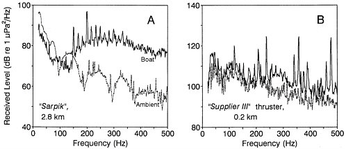
FIGURE 2-1 Received underwater sound spectral densities for two diesel-powered boats: (a) Imperial Sarpik at range 2.8 km, and (b) Canmar Supplier III with 336 kW (450 hp) bow thrusters at 0.2 km. The dotted spectrum is ambient noise before or after boat measurement. Note the different vertical scales in (a) and (b). Reanalyzed from recordings of Greene (1985); analysis bandwidth 1.7 Hz.
SOURCE: Richardson et al., 1995, courtesy of Academic Press.
related tones observed at lower speeds. These spectral characteristics of individual ships and boats can be observed at relatively short ranges and in isolated environments. At distant points, multiple vessels contribute to the background, and it is this superposition of many distant sources that is characterized by broad spectral peaks labeled “usual traffic noise” in the Wenz curves (see Plate 1).
Globally, commercial shipping is not uniformly distributed. The major lanes are great circle routes (unless they extend to very high latitudes) or follow coastlines to minimize the time at sea. Dozens of major ports and several “megaports” handle the majority of the traffic, but in addition there are hundreds of small harbors and ports that host some level of daily seagoing traffic. The U.S. Navy’s Space and Naval Warfare Systems Command defines 521 ports and 3,762 traffic lanes in its efforts to catalogue commercial and transportation marine traffic (Emery et al., 2001).
Other vessels may be found in widely distributed areas of the oceans outside of ports and shipping lanes. These include military craft in fleet exercises, fishing vessels, single vessels such as scientific research ships in a specific location on a one-time basis for measurements, and recreational craft typically near shore.
The contribution from recreational boating to the underwater noise field has not been quantified. Much of this boating activity occurs in shallow coastal waters, environments that are inhabited by many marine mammal species. Information on one aspect of the issue can be obtained from the National Marine Manufacturers Association, which publishes statistics on the number of U.S. boat registrations by state per year and the numbers of boats in various categories (outboard, inboard, sterndrive, personal watercraft, sailboats, and miscellaneous) owned in the United States in a given year (National Marine Manufacturers Association, 2002). For example, the number of boats owned in the United States increased from 15.8 million in 1995 to nearly 17 million in 2001, representing more than a 7 percent increase. Additional information on personal watercraft, a subset of the recreational boating sector, can be obtained from the Personal Watercraft Industry Association (2002). Measurements of the radiated noise from these watercraft are reported, but they pertain to the atmospheric radiated noise because of the potential impact on human coastal communities. Concern for this human impact has led the personal watercraft manufacturers to reduce atmospheric radiated noise levels by 70 percent since 1998. Many of the noise reduction techniques probably also have resulted in a decrease in underwater radiated noise levels. However, some of this 70 percent reduction has been achieved by rerouting the engine exhaust from above the water line to below, so that the overall change in underwater noise is difficult to predict.
Vessel operation statistics are complex to derive because of different criteria for defining ship type in different databases. Indeed, depending on
how different analyses are done, even a single database, such as that produced by Lloyd’s of London, can provide markedly different numbers of ships in the same category. The data mined for Table 2-2 show an increase of the commercial fleet from 72,662 in 1995 to 81,867 in 1999, an increase of 12 percent over four years. The trends all indicate growth consistent with population growth and use of the sea for economic, recreational, and transportation purposes. Economic pressure for oceanic shipping remains strong, and there is no near-term alternative available to move the necessary tonnage of goods and material globally. International economic infrastructure results in more raw materials being exchanged in the trade process. Fishing vessels account for approximately 23,000, or 28 percent of the world fleet. Bulk dry and oil tankers represent nearly 50 percent of the total tonnage but less than 8 percent of the vessel count.
Noise from Individual Ships and Boats
Databases of radiated noise measurements exist for some classes of surface ships. The largest collection of deep-water merchant ship radiated noise measurements probably is the Lloyd’s Registry of London database (Lloyd’s Registry of Shipping; see also Wales and Heitmeyer, 2002). However, limited information is readily available regarding the acoustic signatures of some of the types of commercial vessels listed in Table 2-2. These data often are found in technical memoranda, databases that require international data exchange agreements (e.g., Lloyd’s Registry of Shipping), Navy-related databases, and other sources not readily available to the public and research community.
Every vessel has a unique signature (Figure 2-1), which changes with ship speed, the condition of the vessel, vessel load, the activities taking place on the vessel, and even with the properties of the water through which the ship is traveling (Ross, 1976). However, high-quality shipping noise modeling probably requires only representative source spectra for the different classes of ships (Figure 2-2). Source spectral densities for the five classes of surface ships are used in the ANDES (Ambient Noise Directionality Estimation System) (Renner, 1986a, b; 1988) as well as the RANDI (Research Ambient Noise Directionality) (Wagstaff, 1973; Hamson and Wagstaff, 1983; Schreiner, 1990; Breeding, 1993) models. The curves for the two models differ according to the way the various classes are defined and the modeling approach taken; the levels in ANDES depend solely on the class of ship, whereas ship length and ship speed are used to calculate a scaling factor based on empirically derived power laws in the RANDI model. (The ANDES source spectral densities also are used in the newly developed Dynamic Ambient Noise Prediction System; see Chapter 4). Using the RANDI model, source spectral density levels range from more than 195 dB re 1 µPa2/Hz at 1 m around 30 Hz for fast-moving, large supertankers
TABLE 2-2 Principal Commercial Fleets of the World—by Ship Type Category (GT = gross tons)
|
Ship Type |
No. |
1995 GT |
No. |
1997 GT |
No. |
1999 GT |
|
Liquefied natural gas tanker |
91 |
7,091,934 |
103 |
8,298,330 |
113 |
9,280,153 |
|
Liquefied petroleum gas tanker |
894 |
7,807,087 |
942 |
8,227,819 |
978 |
8,649,191 |
|
Chemical |
2,077 |
12,073,051 |
2,260 |
13,643,913 |
2,456 |
16,310,943 |
|
Crude oil tanker |
1,656 |
118,835,028 |
1,717 |
122,377,669 |
1,782 |
127,875,958 |
|
Oil products tanker |
5,105 |
24,685,537 |
5,216 |
24,729,866 |
5,269 |
26,215,579 |
|
Other liquids |
315 |
415,793 |
347 |
598,154 |
343 |
565,418 |
|
Total |
10,138 |
170,908,430 |
10,585 |
177,875,751 |
10,941 |
188,897,242 |
|
Bulk dry |
4,799 |
128,517,859 |
5,079 |
140,921,192 |
4,881 |
139,408,629 |
|
Bulk dry/oil |
226 |
14,105,815 |
242 |
11,420,914 |
219 |
9,562,092 |
|
Self-discharging bulk dry |
158 |
2,922,535 |
157 |
2,953,916 |
164 |
3,170,689 |
|
Other bulk dry |
982 |
6,148,064 |
1,074 |
6,872,729 |
1,093 |
6,816,236 |
|
Total |
6,165 |
151,694,273 |
6,552 |
162,168,751 |
6,357 |
158,957,646 |
|
General cargo |
17,161 |
56,739,241 |
17,467 |
56,569,318 |
16,880 |
55,981,408 |
|
Passenger/general cargo |
351 |
675,939 |
342 |
602,641 |
348 |
609,892 |
|
Container |
1,763 |
38,742,105 |
2,187 |
48,839,028 |
2,457 |
55,255,401 |
|
Refrigerated cargo |
1,466 |
7,158,402 |
1,443 |
7,145,501 |
7,415 |
7,037,866 |
|
Roll on/roll off cargo |
1,673 |
20,429,523 |
1,742 |
21,978,592 |
1,844 |
25,256,499 |
|
Passenger roll on/roll off cargo |
2,256 |
1,562,021 |
2,425 |
12,121,320 |
2,553 |
12,824,778 |
|
Passenger (cruise) |
287 |
4,979,116 |
328 |
5,877,376 |
345 |
7,194,096 |
|
Passenger ship |
2,236 |
1,190,7921 |
2,500 |
1,239,630 |
2,595 |
1,334,411 |
|
Other dry cargo |
216 |
1,885,770 |
259 |
1,993,038 |
267 |
2,045,037 |
|
Total |
27,409 |
144,080,038 |
28,693 |
156,366,444 |
34,704 |
167,539,388 |
|
Fish catching |
23,111 |
11,005,206 |
22,729 |
10,647,509 |
23,003 |
10,613,938 |
|
Other fishing |
818 |
2,342,715 |
811 |
2,024,838 |
838 |
1,636,874 |
|
Total |
23,929 |
13,347,921 |
23,540 |
12,672,347 |
23,841 |
12,250,812 |
|
Offshore supply |
2,382 |
1,869,241 |
2,370 |
1,960,707 |
2,528 |
2,315,487 |
|
Other offshore |
463 |
2,492,073 |
554 |
3,016,539 |
611 |
4,563,628 |
|
Total |
2,845 |
4,361,314 |
2,924 |
4,977,246 |
3,139 |
6,879,115 |
|
Research |
818 |
1,106,990 |
618 |
1,112,785 |
846 |
1,271,695 |
|
Towing/pushing |
7,721 |
2,085,277 |
8,603 |
2,275,408 |
9,044 |
2,401,953 |
|
Dredging |
1,125 |
1,874,095 |
1,120 |
1,931,933 |
1,121 |
2,279,743 |
|
Other activities |
2,650 |
2,897,862 |
2,659 |
2,746,528 |
2,824 |
2,929,967 |
|
Total |
12,314 |
7,964,224 |
13,000 |
8,066,654 |
13,835 |
8,883,358 |
|
World totals |
72,662 |
321,447,770 |
74,709 |
344,251,442 |
81,876 |
354,510,319 |
|
SOURCE: Lloyd’s Register, Fairplay Ltd., World Fleet Statistics, 2001. |
||||||
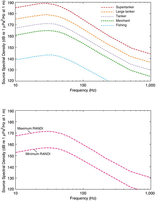
FIGURE 2-2 (a) Modeled surface ship source spectral densities for the five classes of ships used in the RANDI ambient noise model. The curves in each class also are a function of ship length and ship speed; those plotted in the figure pertain to the mean values of ship length and ship speed in each class. (b) A comparison of the maximum and minimum merchant ship source spectral densities from the RANDI model (calculated using the maximum and minimum ship lengths and ship speeds for this class; re Table 2-3). SOURCE: Wagstaff, 1973. Adapted from data from the Naval Undersea Center.
down to 140 dB re 1 µPa2/Hz or less for smaller craft such as fishing vessels (Table 2-3).
Figure 2-2b also shows a comparison of the “merchant” class source spectral densities in RANDI with the mean source spectral density in Wales and Heitmeyer (2002) calculated as the decibel mean over 54 merchant-class source spectral densities. The model of the acoustic source used in Wales and Heitmeyer to derive the source spectral densities from the measured received spectral densities is a vertical line of incoherent point sources, rather than a single-point source, in order to more accurately account for the character of the acoustic source region about the ship propeller. An interesting observation is that the decrease in ship spectral density levels with frequency above 400 Hz has the 5-6 dB/octave dependence as seen in the Knudsen curves for wind-generated noise (see Plate 1). Wales and Heitmeyer also analyzed the variations of individual merchant ship spectra from their mean spectrum; variations are significantly greater below 400 Hz (up to 5.3 dB standard deviation) than above (a standard deviation of about 3.1 dB).
As mentioned previously, ship-generated spectra are composed of a broadband component, predominantly the result of propeller cavitation, and a set of harmonically related tones created both by propeller cavitation (the blade lines) and the machinery on the ship. The broadband and tonal components produced by cavitation account for 80-85 percent of ship-radiated noise power (Ross, 1976). The discussion above pertains to the character of the broadband component. Source-level models also have been developed for the propeller fundamental blade rate line occurring predominantly in the 6-10-Hz band for the world’s merchant fleet (Gray and Greeley, 1980).
Acoustic signature data are available for some oceanographic research ships and boats. Although they may be important locally, noise levels are typically so low they are unimportant in the general acoustic environment of the world’s oceans. There is a significant literature dealing with the effects of fishing vessel noise on fish populations on which marine mammals may depend (Mitson, 1995). Observed responses of marine mammals to boats, not just fishing boats, are discussed in Chapter 3. Signature data are not readily available for most survey or observation vessels, although some examples are presented in Richardson et al. (1995) and as unpublished documents and reports. A sampling of whale-watching boat signatures is available in the published literature (e.g., Richardson et al., 1995; Erbe, 2002).
Extensive acoustic signature data exist for military surface ships. Individual vessel signature data resources are classified and held in government agencies such as the Naval Research Laboratory and cannot be used in this study. The U.S. Navy does post vessel descriptions as well as current deployment numbers on its Web site.
TABLE 2-3 Source Spectral Densities for Commercial Vessels Underway for Several Frequencies
|
|
Source spectral density (dB re 1 µPa2/Hz at 1 m) |
||||||
|
Ship Type |
Length (m) |
Speed (m/s) |
10 Hz |
25 Hz |
50 Hz |
100 Hz |
300 Hz |
|
Supertanker |
244-366 |
7.7-11.3 |
185 |
189 |
185 |
175 |
157 |
|
Large tanker |
153-214 |
7.7-9.3 |
175 |
179 |
176 |
166 |
149 |
|
Tanker |
122-153 |
6.2-8.2 |
167 |
171 |
169 |
159 |
143 |
|
Merchant |
84-122 |
5.1-7.7 |
161 |
165 |
163 |
154 |
137 |
|
Fishing |
15-46 |
3.6-5.1 |
139 |
143 |
141 |
132 |
117 |
|
SOURCE: Adapted from Research Ambient Noise Directionality (model) (RANDI) source-level model in Emery et al. (2001) and Mazzu ca (2001). |
|||||||
Pleasure craft do not contribute significantly to the global ocean acoustic environment but may be important local sources of underwater noise. High-speed ocean yachts are expected to be sources of high noise levels but are sufficiently small in number as to represent significant sources only local to the individual craft. Results from a recent study of source signatures from outboard, inboard-outboard, and inboard powerboats shows that source levels for the largest amplitude narrowband tones typically range between 150 and 165 dB re 1 µPa at 1 m and the broadband radiated energy, which is engine RPM dependent, has maximum source spectral density levels in the 350-1,200-Hz band of 145-150 dB 1 µPa2/Hz (Bartlett and Wilson, 2002). Additional examples of individual ship signatures in these classes can be found in Richardson et al. (1995).
Future Trends in Shipping
Although the number of vessels and tonnage of goods shipped are increasing (e.g., a nearly 30 percent increase in volume shipped by the U.S. fleet over the past 20 years; 1,793.9 million metric tons [mmt] in 1980 to 2,331.6 mmt in 2000) (U.S. Maritime Administration, 2002), the relative distribution of numbers of ships among the various classes is not expected to change remarkably in the future. If dramatic changes are made to the shipping fleet, they likely will be mandated by economic forces such as more efficient or cheaper propulsion systems, faster ships, or hull configurations that allow more bulk tonnage. Any one of these changes could have a significant impact on a ship’s radiated noise characteristics. A discussion of the long-term trends in shipping contributions to ocean noise is presented later in this chapter.
Marine Noise Generated by Oil and Gas Industry Activities
Oil and gas industry activities may be divided into five major categories: (1) seismic surveying, (2) drilling, (3) offshore structure emplacement, (4) offshore structure removal, and (5) production and related activities (including helicopter and boat activity for providing supplies to the drilling rigs and platforms). Offshore seismic surveying, the predominant marine geophysical surveying technique employed by the oil and gas industry, uses intentionally created sound. The last four activities listed create primarily unintentional noise and will be discussed in less detail. The noise levels associated with oil and gas production are typically much lower than those involved in seismic surveying (see Richardson et al., 1995).
Offshore oil industry activities have a patchy distribution along the world’s coastlines, ranging from about 72o N latitude to about 45o S latitude. Seismic surveying activity and oil and gas production have taken place off the coasts of North and South America, Africa, Europe, Asia, and
Australia. Activity levels associated with well drilling and seismic surveying by the oil and gas industry are monitored by various industry trade and database companies and published on a monthly basis in various trade journals, such as Hart’s E&P, Journal of Petroleum Technology, Oil and Gas Journal, Offshore, and World Oil. The companies actually performing the work provide the numbers about these activity levels to the database companies.1
Seismic Reflection Profiling
Seismic reflection profiling encompasses a variety of methods, all of which use sound to relay information about geological structure beneath the surface of the earth. The oil industry relies on the extensive use of seismic reflection profiling to provide unique information about the rocks that extend beneath the seafloor, down to depths exceeding 10 km. Seismic reflection profiling, which includes what is commonly called three-dimensional (3D) seismic, is also used by academic and government groups, as well as the mining, environmental consulting, and other industries, to gather information about subsurface rock properties. The major operational elements in industrial marine 3D seismic reflection surveying are (1) the seismic vessel, typically about 100 m long by 30 m wide; (2) one or two air-gun arrays towed about 200 m behind the seismic vessel; and (3) cables, called streamers, containing large numbers (on the order of a few thousand) of hydrophone sensors towed behind the seismic vessel. Current technology uses streamers up to 12 km long to record the echoes returning from the subsurface (Figure 2-3). In the open marine environment, air-guns are the most commonly used sound source, but explosives buried in drilled holes are used to acquire similar data in waters shallower than about 4 m.
Marine seismic reflection profiling currently relies on the use of arrays of air-guns. These arrays have replaced the explosive charges that previously were used as sources.2 Air-guns release a volume of air under high pressure, creating a sound pressure wave that is capable of penetrating the
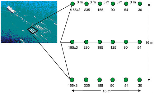
FIGURE 2-3 Schematic diagram of an air-gun array. A total volume of 3,397 cu. in. is shown. This array has three subarrays (each line of circles) and uses 24 air-guns. Each circle represents an air-gun, except for the circles at the head of each array, which represent three-gun clusters. The nearest number represents the volume of air expelled by individual air-guns in cubic inches.
seafloor to determine substrata structure. Each complete air-gun array used in the seismic industry will typically involve 12-48 individual guns. Most of the seismic industry uses air-gun arrays with operating pressures of 2,000 psi (equal to 13.8 million pascals) and are typically about 20 m by 20 m.
The acoustic pressure output of an air-gun array is (1) directly proportional to its operating pressure; (2) directly proportional to the number of air-guns, all else being equal; and (3) proportional to the cube root of the volume. For example, an 8,000-cu.-in. (0.131 m3) array has a 3.4-dB greater output than a 2,500-cu.-in. (0.041 m3) array having the same number of guns.3 The acoustic pressure signal of air-gun arrays is focused vertically, being 12-15 dB stronger or more in the vertical direction for some arrays in use today. The ability to focus the sound output in the vertical direction is a function of the total array aperture in both the fore-and-aft and side-to-side directions and the number of air-guns in the array
(Plate 4). Vertical output can be maximized while minimizing output in the horizontal plane through the use of arrays incorporating more small air-guns rather than fewer larger air-guns.
The literature, including both that published by the seismic exploration industry and by bioacousticians, refers to back-calculated levels of up to 260 dB re 1 µPa at 1 m for the maximum output pressure levels [zero-to-peak, subtract about 10 dB to obtain root mean squared (RMS) value, per W. J. Richardson, personal communication, 2002] of industry air-gun arrays (Richardson et al., 1995; Dragoset, 1990). The back-calculation is valid for point sources, not ones that measure 20 m on a side, so that the 260 dB should be used to calculate sound pressures in the vertical far field. The far-field distance is a function of the array dimensions, the speed of sound in water, and the frequency of the source. The maximum pressure level an animal could experience from an air-gun source in use today in the seismic industry will be in the range of 235-240 dB re 1 µPa (RMS). The location where this level of sound is attained will be vertically beneath the air-gun array, generally near its center, but the exact location and depth beneath the array are dependent on the detailed makeup of the array, the water depth in which the array is operating, and the physical properties of the seafloor above which the array is operating (Dragoset, 2000).
The peak amplitude of an air-gun array is also a function of the frequency (Figure 2-4). The peak pressure levels emitted from commonly used seismic industry air-gun arrays are in the 5-300 Hz range. The guns are towed at a speed around 5 knots (2.6 m/s) and are fired about every 10-12 seconds. A typical seismic operation includes a series of parallel passes by a vessel towing one or two air-gun arrays and 6-10 streamers. Turning typically takes about two hours, and the air-guns are shut down during this maneuver. In addition to this turning period, the air-guns do not operate when the vessel is in transit to and from the survey site, when sufficiently bad weather occurs, when streamers are being deployed or retrieved, or when critical equipment fails. Given these constraints, air-guns are generally firing less than 40 percent of the time the vessel is underway (Philip Fontana, personal communication, 2002).
Marine seismic crews are much more efficient today than they were 10 years ago, since more and longer streamers are towed now than in the past (DeLuca, 2000; Eng, 2001; Maksoud, 2001). The acquisition footprint (0.25 times the total length of the streamer times the total distance from the starboardmost streamer to the portmost streamer) can be as much as 4.24 km2. In other words, a seismic crew can get into and out of a specific area much more quickly than in times past because fewer tracks are required, given the wider coverage (swath) per track. The use of seismic time-lapse monitoring for reservoir management (repeating seismic surveys to monitor changes in a hydrocarbon reservoir over months and years) means that
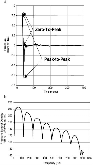
FIGURE 2-4 Acoustic signal of a 4,550 cu. in. air-gun. (a) Typical pulse created by the firing of an air-gun array. The high-amplitude portion of the pulse lasts about 20 ms. (b) An amplitude spectrum of an air-gun signal. This plot shows pressure levels as a function of frequency for a signal generated by a 4,550-cu.-in. air-gun array. Courtesy of Philip Fontana, Veritas DGC.
more seismic surveys are likely to be shot over producing fields than was true in the past.
Noise Generated by Other Hydrocarbon Industry Activities
Drilling techniques employed by the oil and gas industry require a wide variety of equipment (Box 2-3). At any given time, it can be assumed that representatives of each of these types are in use somewhere in the world (Table 2-4). When drilling is taking place, auxiliary noise is generated, created by activities including supply boat and support-helicopter movements. The worldwide offshore mobile rig count can vary over time as a result of business conditions in the oil industry (Figure 2-5). A comparison of rig counts (Table 2-4, Figure 2-5) highlights the differences in reporting from the groups. These graphics illustrate the overall numbers of rigs of all types operating at a given time, an idea of year-to-year variability, and a current distribution of rigs for different areas around the world.
Jack-ups are the most commonly used offshore drilling equipment, followed closely by the use of platform rigs (see the Offshore Rig Locator published monthly by the ODS-Petrodata Group). The sound pressure levels created by the different drilling methods are not well known. Richardson et al. (1995) present a small amount of data, mostly recorded from the monitoring of projects along the North Slope of Alaska and the adjoining coast of Canada. In general, drill ships are the noisiest type of drilling equipment being used, with a maximum broadband source pressure level across the 10-Hz to 10-kHz band of about 190 dB re 1 µPa at 1 m (RMS) (Richardson et al., 1995). Drill ships are expected to be the noisiest
|
Box 2-3 Oil and Gas Extraction Platforms Platform rigs: permanently mounted rigs located on stationary production structures Semisubmersibles: mobile, steel-decked structures whose hollow support structures do not rest on the seafloor Jack-ups and submersibles: mobile, steel-decked structures whose legs or other support structures rest on the seafloor Drill ships: ships with drilling capabilities Drill islands: artificial islands upon which drilling rigs are placed, constructed in areas normally covered by ice substantial portions of the year |
TABLE 2-4 International Offshore Mobile Working Rig Count
|
Location |
January 2002 |
December 2001 |
January 2001 |
|
Canada |
7 |
7 |
6 |
|
Europe |
71 |
61 |
53 |
|
Middle East |
37 |
37 |
30 |
|
Africa |
20 |
18 |
23 |
|
Latin America |
46 |
47 |
45 |
|
Asia Pacific |
61 |
59 |
55 |
|
United States |
126 |
123 |
174 |
|
Total |
368 |
352 |
386 |
|
SOURCE: Hart’s E&P, April 2002. |
|||
because the hull is an efficient transmitter of all of the ship’s internal noises, and the ships do not anchor but use thrusters to remain on location, resulting in propeller noise much of the time during the drilling operation. Research is needed to make accurate measurements of the sound pressure levels generated by various drilling techniques.
The compilation of drilling activity numbers over time with a conventional geographic breakdown as illustrated by Table 2-4 may not be particularly useful to describe the drilling ensonification of the oceans. Neither changes in relative percentages of the different drilling technologies being used nor changes in the distribution of activities between shallow water and
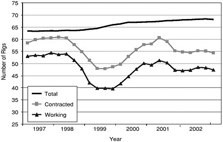
FIGURE 2-5 Worldwide offshore mobile rig numbers from 1997 to present. This figure does not include rigs permanently located on platforms, of which there were 139 contracted as of March 4, 2003. SOURCE: ODS-Petrodata, Houston.
deep water are reflected in general oil rig estimates. Rapid changes in drilling technology and equipment are likely to change the noise generated and are not included. Sound pressure level measurements are needed to conclude how these changes in oil industry techniques affect ocean noise.
Offshore structure emplacement will create some localized unintentional noise for relatively brief periods of time. Because a few large structures that will span relatively great water depths are emplaced each year, extremely powerful vessels are required to transport them from the point of fabrication to the point of emplacement. This activity lasts for a few weeks and currently does not occur more often than 8–10 times per year. The installation of subsea structures, primarily in deep-water sites, is becoming more commonplace. Measurements of the sound pressure levels associated with such activity have yet to be made.
Additional noise is generated during oil production activities, which can include borehole logging, casing, cementing, perforating, pumping, pipe laying, pile driving, ship and helicopter support, and others to support rig and platform work. Impulsive hammering sounds created by installation of conductor pipe resulted in received sound levels of 131-135 dB re 1 µPa recorded 1 km from the source (see Richardson et al., 1995). Assuming transmission loss resulting from spherical spreading, this will translate to 195 dB re 1 µPa at 1 m, with the peak amplitudes occurring at around 40 and 100 Hz.
Oil Industry Noise—Future Trends
Oil and gas industry activities occur along many continental margins between 72° N latitude and 45° S latitude. The major areas of current oil industry activity include northern Alaska and extreme northwest Canada, the east coast of Canada, U.S. Gulf of Mexico, Mexican Gulf of Mexico, offshore Venezuela, offshore Brazil, offshore West Africa, offshore South Africa, North Sea (most sectors), Middle East, northwest Australia, New Zealand, southern China, Vietnam, Malaysia, and Indonesia. It is unlikely that any major shifts in gross patterns of where this industry operates will take place in the near future.
Noise levels associated with new exploration activities may be more noticeable when they occur in relatively quiet areas with little human activity. Recent new exploration areas include the deep-water U.S. Gulf of Mexico and deep-water offshore of West Africa, both of which basically have become active in the past 5-10 years. Local and global economic changes can abruptly modify exploration plans, so noise levels that are affected by exploration activities can change rapidly. How quickly drilling activity is turned off and on depends in large part on which specific oil companies are operating in a particular geologic province or basin. How fast seismic surveying activity is turned off and on depends on global eco-
nomic factors, as well as local economic conditions, and again on which specific oil companies are in a given area.
Oil and gas production is moving into water depths up to 3,000 m. Those depths will require the use of drill ships and most likely require the use of floating production, storage, and off-loading systems that involve the use of oil tankers, most likely on nearly a weekly basis, since high production rates are needed to justify the expense of deep-water fields. Therefore, the deep-water fields may be a source of greater noise than the shallow-water fields have traditionally been, at least in terms of base noise levels. The Minerals Management Service in the United States is now recognizing this as a growing issue.
Sonars
Sonar (sound, navigation, and ranging) systems use acoustic energy to characterize physical properties and locate objects beneath the ocean surface. The wide range of applications requires systems that vary greatly in engineering specifications and deployment strategies. Sonar systems have both military and civilian applications and can be divided into low-frequency (<1 kHz), mid-frequency (between 1 and 10 kHz), and high-frequency (>10 kHz). Generally, military systems exist for all frequency ranges, while civilian systems are confined to the higher frequencies.
Military Sonars
Military sonars are typically operated at higher power levels than civilian sonars and are used for target detection, localization, and classification. Military low-frequency sonars are used for surveillance and are designed to gather information over large areas. If conditions permit, these sonars can collect information over entire ocean basins. The mid-frequency military systems are tactical sonars and are designed to look over tens of kilometers for the localization and tracking of targets. Military high-frequency systems are either weapons (torpedoes and mines) or counterweapons (mine countermeasure systems or antitorpedo devices) and are designed to perform over hundreds of meters to a few kilometers.
Active sonar technology, currently deployed by the navies of the world and undergoing further development, seeks targets by sending out high-energy acoustic pulses and recapturing the echo. Characteristics of the echo provide information on the objects that reflect and scatter the pulses. The class of surveillance sonars presently in the fleet is designed to locate targets, primarily submarines and to some extent surface ships, at tens to hundreds of kilometers away to provide early alerts of potential threats to navy vessels. The U.S. Navy’s Surveillance Towed Array Sensor System Low Frequency Active (SURTASS-LFA) system utilizes a vertical line array
of up to 18 source projectors operating in the frequency range of 100-500 Hz. The source level of each projector is approximately 215 dB re 1 µPa at 1 m (Johnson, 2001). In addition, the U.S. Navy reports that the hull-mounted AN/SQS-53C tactical sonars can generate pulses in the 1-5 kHz band and have been operated at source levels of 235 dB re 1 µPa at 1 m and that the AN/SQS-56 sonars generate pulses in the 5-10 kHz band and have operated at 223 dB re 1 µPa at 1 m source levels (Evans and England, 2001). High-frequency military sonars (above 10 kHz) are used for weapon and counterweapon location at ranges of tens to thousands of meters. The sonars are operated in a variety of modes, different signal types, and different signal lengths and strengths but typically over a relatively narrow frequency range. They can be used to generate broadband signals in which a wide range of frequencies are transmitted simultaneously, but it is not common to do so.
The use of military sonars typically is limited to operational areas, a small portion of the total ocean space (Lloyd’s Register, 2001). If war situations are excluded, the remaining areas of military activity are well defined and the level of activity is also well defined and episodic; typical U.S. Navy individual ship exercises last a few hours to a few days, predeployment and battle group exercises normally last 10-12 days and involve a full carrier battle group or amphibious-ready group, and the duration of large multinational fleet exercises is up to a month, but these occur only every other year or so. The total number of military ships extant on the globe numbers in the thousands, but use of military sonar systems is limited to hundreds.
Other military active sonars include communication sonars for inter-platform information exchange, depth sounders, sidescan sonars for seafloor mapping, and variants of the communication sonar that are used for device activation and event initiation, for example. Mine-hunting systems are high-frequency systems, ranging from tens of kilohertz for detection to hundreds of kilohertz for localization. The systems are highly directional and use pulsed signals.
Commercial Sonars
Commercial sonar systems are designed for special purposes such as depth sounding, fish finding, and obstacle detection. Typically, they operate at higher frequencies, project lower power, and have significant spatial resolution with narrower beam patterns and shorter pulse lengths than military sonars. Characteristics of the underwater transducers used in these commercial sonar systems, as well as in military sonar systems, can be obtained from the transducer manufacturers, including the International Transducer Corporation, Reson, and Massa Products Corporation. Commercial sonars typically operate in a narrow frequency band with a center
frequency between 1 and 200 kHz or more, depending upon the application. The source levels of some of these sonar transducers can reach values of 250 dB re 1 µPa at 1 m (e.g., model TR-208A by Massa Products Corporation) (Massa Products Corp., 2002). These source levels are sufficiently high that sonar performance in shallow water becomes limited by cavitation (Urick, 1975).
Commercial depth sounders and fish finders typically are designed to focus sound in the downward direction, although forward-looking sonars also are available. A common type of fish finder/echosounder (e.g., model LS-6000 from Furuno) operates at two frequencies, 50 kHz and 200 kHz, with output power on the order of 1 kW (201 dB re 1 µPa at 1 m) at a duty cycle of 0.1 percent (0.2 ms pulse every 0.2 s). These frequencies are too high to be audible to fish; however, 50 kHz certainly falls within the range of hearing sensitivity of many marine mammal species. Even if only a small fraction of the 17 million boats owned in the United States in 2001 (National Marine Manufacturers Association, 2002) and the 80,000 vessels in the world’s merchant fleet as of 1999 (Table 2-2) are equipped with commercial sonar systems, the potential exists for these systems to adversely impact the marine environment. Depth sounders typically operate in nearshore and shallow waters. However, fish finders are used in biologically productive areas in both deep and shallow waters that are likely to contain marine mammals.
According to the Pew Oceans Commission (2002), the mortality caused by the unintended capture during commercial fishing operations (“bycatch”) exceeds sustainable levels for 13 of the 44 marine mammal species that suffer high mortality rates as a result of human activities. Low-power acoustic deterrent devices (ADD) are used in some fisheries in attempts to reduce this bycatch. Good evidence exists that these “pingers” are effective, at least for some marine mammal species. High-power ADDs (sometimes called acoustic harassment devices or AHDs) are designed to be sufficiently high level to exclude marine mammals, usually pinnipeds, from areas such as aquaculture sites, sections of river systems where migrating salmonids are vulnerable, and some fishing equipment. Whereas the low-power “pingers” have maximum source levels typically between 130 and 150 dB re 1 mPa at 1 m, the high-power AHDs have source levels in the 190-200 dB re 1 µPa at 1 m range. Both types generate a series of pulses, each lasting from 10 to 500 ms with interpulse periods ranging from negligible (i.e., continuously repeated transmissions) up to 10 s. The signals have frequency content in the 5-30-kHz band and some extend up to 160 kHz, which is sufficiently high to be outside the range of audibility of most species of fish.
In the United States, attention turned to the problem of bycatch more than a decade ago and resulted in an increase in the use of acoustic deterrents. Amendments to the Marine Mammal Protection Act during its reau-
thorization in 1994 included provisions to try to reduce marine mammal bycatch. U.S. fisheries now are placed in one of three categories:
-
those with frequent serious injuries and death of marine mammals,
-
those with occasional serious injuries and death, and
-
those unlikely to cause serious injury or death.
The number of U.S.-registered vessels in each of these categories in each of the various U.S. fisheries is published at least yearly in the Federal Register. The most recent report (McKeen, 2002) shows about 14,300 vessels in category I, with 188 of these off the California and Oregon coasts, about 14,000 in the Atlantic, and 100 or so in the Gulf of Mexico and the Caribbean. The category II vessels number more than 25,300 with 7,364 off the West Coast of the United States, more than 17,950 in the Atlantic, and 50 in the Gulf of Mexico. Fishing boats that are in categories I and II must follow certain procedures, including registering yearly with the National Marine Fisheries Service for authorization to incidentally take marine mammals during fishing activities, allowing designated observers aboard when requested, and following “take reduction” plans developed for that fishery. Take reduction plans for some fisheries were put in place as early as 1997-1998, and some of these plans have included the deployment of low-power ADDs. As a result, the use of these pingers in the U.S. commercial fishing fleet has jumped in the past 4-5 years and continues to change with further development and modification of the various fisheries’ take reduction plans.
Fishing nets with pingers exclude porpoises from their immediate vicinity. Although bycatch is thereby reduced, concerns have arisen that pingers could lead to significant habitat exclusion if used in sufficient numbers. In contrast, AHDs are sufficiently high level that they could actually damage the hearing of marine mammals exposed at close range. Pinnipeds that are highly motivated to prey on the fish being protected are particularly susceptible. In addition, AHDs used at aquaculture facilities have been shown to exclude nontargeted species, especially odontocetes. For example, Olesiuk et al. (2002) have shown that porpoise densities were significantly reduced when ADDs were in operation. No porpoises were found within 400 m of the device, and the sighting rates between 2.5 and 3.5 km were 10 percent of the control rates.
Underwater Sound Sources in Basic Ocean Acoustics Research
This section summarizes the characteristics of underwater sound sources used in basic ocean acoustic and acoustical oceanography research programs in the United States. Basic science programs in seismology that have seagoing experimental components involving the deployment of underwa-
ter seismic sources are not discussed here. Rather, the characteristics of seismic air-guns and air-gun arrays often used in these experiments are discussed under the Seismic Reflection Profiling section.4 In addition, explosive charges used as seismic sources are discussed under the Explosive Sources section in this chapter. Active acoustic experiments, those involving acoustic signal transmissions, in advanced development programs for the operational navy also are not covered here because of their classified nature. They are best considered part of the operational navy activities discussed in the Military Sonars section.
Almost all of the basic ocean acoustics research programs in the United States are sponsored by the Office of Naval Research (ONR). Fewer than a dozen or so experiments are conducted each year and typically last one to three weeks. The sound sources in these experiments primarily are commercially available transducers, sometimes with small changes in design or deployment geometry, but also a few specially designed sonars are used to meet specific research objectives. In addition, sources often are rented from the Underwater Sound Reference Detachment (USRD). For example, a popular sound source from USRD that is used in low-frequency acoustics experiments is a Type J15-1 source. It is a moving coil-type device designed to transmit signals in the 30-900 Hz band with a maximum source level of approximately 170 dB re 1 µPa at 1 m (Ivey, 1991). A wide variety of waveforms are transmitted by these sonars over a wide range of frequency bands, source levels, and duty cycles because of the large number of research questions addressed in these programs. Explosive charges sometimes are deployed, although their use by the research community has been decreasing, partly because of safety and environmental concerns but also because of the lack of control over and the nonreproducible nature of the source waveform and the detonation depth. The spatial extent of the signals transmitted in most of these experiments, other than the basin-scale acoustic tomography experiments discussed below, are local in nature, less than a few tens of kilometers. Although the experiments have been conducted in various parts of the world, U.S. experiments typically occur in U.S. territorial waters.
The most widely known ocean acoustics research program is the Acoustic Thermometry of Ocean Climate (ATOC) program. It has received a high level of attention from regulatory agencies, the public, and the scientific community. The characteristics of the ATOC source signals have been documented in the two previous NRC reports on low-frequency
sound (NRC, 1994, 2000). The source, deployed at a depth greater than 800 m, has a source level of 195 dB re 1 µPa at 1 m. Modern-day ATOC experiments and the few other recent basin-scale acoustic tomography experiments have spatial extents of hundreds of kilometers. These experiments are able to probe the properties of the ocean out to basin-scale ranges to thousands of kilometers because the transmitted signals are long and complex. Therefore, matched filtering of the received signal with the transmitted signal provides significant processing gain (the AG term in Equation 1-3).
Since the start of the ATOC program and the controversy surrounding it, ocean acoustic experimental programs have undergone an increasing degree of scrutiny. The ONR now requires all ONR-sponsored experimental research programs involving underwater acoustic transmissions to follow the planning process specified in the National Environmental Policy Act (NEPA). The purpose of this process is to clearly identify and mitigate against any potential effects of acoustic transmissions, as well as all other experimental activities, on the marine environment and to establish if an environmental impact statement must be prepared. All federal and relevant state environmental laws must be followed, including the Marine Mammal Protection Act, the Endangered Species Act, and the Magnuson-Stevens Fisheries Conservation and Management Act, as well as other laws, regulations, and executive orders.
Future Trends in Sonar Use
Commercial sonars will continue to proliferate in the oceans. Their acoustic characteristics will not change significantly, since absorption limits the frequency at the high end, physical size is a limitation at lower frequencies, and the properties of the water column itself at the very shallow depths of hull-mounted systems limit the maximum acoustic power output as a result of cavitation (Urick, 1975). However, acoustic power output is not a limiting factor for most commercial sonar applications in most environments. Potentially, research to increase the power of military sonars could continue, but operational requirements for higher power will require difficult research. Current materials and structural configurations cannot survive the extreme electric fields and displacements necessary to produce more acoustic power. An alternative approach is to deploy arrays of sources that circumvent these constraints but have limitations of their own, for example, they are difficult to deploy or difficult to maneuver while being deployed.
Perhaps the most uncertain are new applications for sonars. The ocean is still poorly understood, both in economic potential and in its role in the well-being of our planet. As terrestrial resources dwindle, the pressure to
understand, map, and explore the ocean will rise dramatically. A variety of sonar devices provide the most effective methods, so research, development, and increasing use of new sonar tools are likely.
Sonars are designed and built worldwide—their characteristics are well understood and calibrated, and these data are generally available. The impacts on ocean organism populations are unknown. To what characteristics do marine mammals react—are they particularly susceptible to certain parameters such as rise time, power, signal length, particular frequencies, or rate of repetition? These characteristics may be modified to minimize effects on marine life without detracting from the purpose of the tool.
Explosive Sources
Explosive sources are broadband with very high zero-to-peak source levels. In fact, the highest zero-to-peak pressure levels from man-made sources probably were created by the nuclear tests conducted in the ocean, in the atmosphere over the ocean, and on oceanic islands in the past half century. In the case of chemical explosive devices, they are physically small, portable, and easily deployed from a variety of platforms. They have traditionally been used for research purposes and some years ago were incorporated into a naval antisubmarine warfare sensor system. Explosives are also used in construction and removal of unwanted undersea structures. In the past, they were used as sources in seismic exploration, but modern-day surveys employ air-gun arrays. However, a few geophysical research programs continue to use explosives.
Military vessels undergo a series of tests to determine their ability to withstand explosions near the hull. Trials, known as ship shock trials, are carried out on every class of U.S. military vessel hull prior to commissioning. During a ship shock trial, explosives are detonated near the hull and hull stress is measured. While the pressure waves generated by this source are very large, this noise source is extremely episodic, since few ship shock trials are conducted annually. Large explosives are also used occasionally for the “sinkex” (a ship hulk sunk with a torpedo warshot) weapon tests during development and for test firing of operational stores for military readiness exercises.
A significant literature base has resulted from research into the spectral and amplitude characteristics of chemical explosives (Figure 2-6). The source level and spectral structure, which is relatively flat, of an explosive device can be predicted using the charge weight and depth of detonation (Table 2-5). For example, the zero-to-peak source pressure level, SL(0–pk), of the initial shock wave, the largest-amplitude component in the detonation time series created by a high explosive, is given by the formula
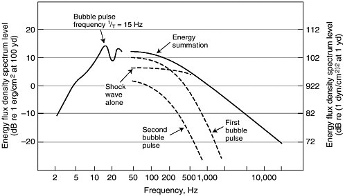
FIGURE 2-6 The spectrum of the acoustic signal from an underwater explosion. The quantity labeled “energy flux density” actually is the instantaneous pressure amplitude squared summed over the duration of the signal, as discussed in the Glossary. To convert the units on the right-hand vertical axis from dB re 1 [(dynes/ cm2)2](sec) at 1 yd into dB re 1 (µPa2)(sec) at 1 m, approximately 100 should be added to the values so that the resulting axis extends from 162 to 222 dB re 1 (µPa2)(sec) at 1 m. These spectral levels pertain to a 1-lb. charge detonated at a depth of 20 fathoms (36.6 m) and are equal to the actual source level at each frequency for a signal of 1-sec duration. The corresponding broadband zero-peak pressure level at 1 m from the source for the initial shock wave from a 1-lb. charge of TNT is 272 dB re 1 µPa at 1 m, as given by Equation 2-1 in the text. The plot shows the addition of the shock-wave and bubble pulse energies at frequencies greater than 1/T, with T equal to the time interval between the shock wave and the first bubble pulse.
SOURCE: Urick, 1975. Reprinted with permission from the Acoustical Society of America.
SL(0–pk)(dB re 1 µPa at 1 m) = 271.8 dB + 7.533*log(w) (2-1)
where w is the charge weight in pounds. The third column of Table 2-5 provides some examples from the use of Equation 2-1.
Industrial and Construction Contributions to Marine Noise
The range of activities in this category is extremely broad, ranging from power plants located near the seaside to pile driving, dredging, shipyards, canal lock structure operations, and general harbor daily functions. The coupling of this energy, which is a combination of terrestrially based to shoreline and nearshore, into the marine environment is poorly understood.
TABLE 2-5 Zero-to-Peak Pressure Level and Spectral Level at 1 kHz of Pressure Amp Squared Times Duration for High Explosive Detonated at 40 m Depth
|
TNT (lb.) |
Spectral Level at 1 kHz of Pressure Amp Squared Time Duration (dB re 1 µPa at 1 m) |
Zero-to-Peak Pressure Level at 1 m (dB re 1 µPa2s at 1 m) |
|
1 |
192 |
272 |
|
10 |
200 |
279 |
|
100 |
207 |
287 |
|
SOURCE: Urick, 1975. Courtesy of McGraw-Hill. |
||
This broad range of activities produces a range of source levels and acoustic patterns:
-
pile driving (impulsive, very high amplitudes),
-
power plants (very strong 60-cycle and harmonics),
-
industrial (tones at frequencies of machinery operating speeds),
-
dredging [both shipborne machinery and mechanical motion (suction and earth-moving devices, possible explosive use)], and
-
power-generating windmills.
A typical spectral structure is broadband with the superposition of a number of lines originating from reciprocating machinery or engines.
Some measurements of the underwater sounds created by these types of sources have been presented in the open literature (e.g., Richardson et al., 1995). Additional measurements are contained in various technical reports and memoranda. It would be useful to gather these measurements together into one easily accessible place (as the committee recommends) for use by the scientific and regulatory communities as well as others. Note, however, that the coupling of land-based vibrations and very nearshore sounds into the offshore underwater acoustic field is highly dependent on the geology, morphology, and length of the land-based portion of the propagation path. Therefore, measurements made in one offshore area are not necessarily applicable to other offshore areas. Numerical modeling of the coupling between land-based vibrations and the ocean acoustic field is a subject of current research. This uncertainty associated with the coupling process makes an assessment of the overall impact of these sounds on the marine environment difficult. However, of greater importance is to understand the potential impact of a given noise source in its actual geological setting on the marine ecosystems that are located nearby. At present, the evaluation for land-based and very nearshore sources probably is best done using actual underwater acoustic measurements in the region of interest.
LONG-TERM TRENDS IN OCEAN NOISE
One of the most important and challenging issues that emerges in an examination of ocean noise and its effects on marine life is the quest to determine any long-term trends in the overall levels of sound in the sea. How has noise in the sea increased with time since the 1850s through increased industrialization and related maritime activities? What parameters, other than direct noise measurements, might be related to the overall sound levels produced by the myriad of sources described? What, if any, modeling capabilities exist to predict ocean noise levels and other noise characteristics in the decades to come? Is there any hope that humans might influence these predicted changes through time by introducing appropriate mitigation measures? Answering these questions holds enormous significance for life in the sea; after all, long-term changes in background noise levels may influence animal behavior and impact the very existence of a particular species. Long-term trends are particularly insidious in that they result from the gradual accumulation of effects over much shorter periods of time for which these effects may appear to be imperceptible.
Although the importance of assessing long-term trends in ocean noise levels is clear, there is a remarkable dearth of theories or data addressing this topic. Commercial shipping noise is apparently the only area in which it is possible to make informed comments concerning long-term trends, and even in that case, the data sets are very limited and the discussion is usually speculative. The focus on shipping implies an emphasis on frequencies of a few hundred hertz and below and a geographical bias toward the northern hemisphere, where most of the dominant shipping lanes exist. In this section, the first attempts to estimate the preindustrial noise background by examining measurements in areas of the South Pacific with extraordinarily low ship traffic are described (Cato, 1997, 2001). The addition of the anthropogenic component of noise during the Industrial Revolution, principally the result of shipping, is reviewed, followed by a summary of existing data on long-term trends in shipping noise levels and a discussion of various indicators for evaluating and predicting shipping noise levels. Finally, speculations on the long-term trends in ocean sounds other than those from shipping are presented. Recommendations for future research to measure and predict long-term trends in ocean noise are listed in Chapter 5.
Preindustrial Noise
One approach to modeling long-term trends is to hypothesize that the overall background noise level remained essentially constant until the onset of the Industrial Revolution in 1850. At that time, land-based industrial activities began to escalate rapidly and resulted in an enormous increase in the use of ships under power to transport goods and provide services over
the oceans. Other related, though less significant, developments were the powering of the world’s naval vessels and the expansion of coastal and offshore construction activities. Additional, though also secondary, sources of anthropogenic noise that emerged much later (primarily during the past 50 years) were those produced by offshore oil exploration and drilling activities, naval sonars, and acoustical oceanographic research. This model is based on the assumption that the noise contributed by natural physically generated and biological sources is independent of time and that human-generated noise prior to the Industrial Revolution was negligible. In fact, this assumption is open to debate, since there is some evidence that global climate change effects have resulted in higher sea states (Bacon and Carter, 1993; Graham and Diaz, 2001); these could potentially cause an increase in the noise levels generated by breaking waves over time. This effect is very likely of secondary importance, however, and therefore the model in which commercial shipping provides the primary time-dependent influence on long-term noise levels is adopted here.
The waters surrounding Australia provide a unique opportunity to estimate preindustrial noise levels. Shipping densities in some areas are extremely low or negligible. This situation provided Cato (1997b, 2001) with the opportunity to determine the “usual lowest ocean noise” level from an extensive suite of measurements (Plate 5). There are several striking features that appear in these data. First, the lowest noise level decreases monotonically from 55 dB re 1 µPa2 per Hz at 10 Hz to 30 dB re 1 µPa2/Hz at 11 kHz. Second, the ship traffic noise data indicate values as high as 80 dB re 1 µPa2/Hz at 20 Hz in the Tasman Sea, “and these approach the traffic noise levels of North American and European waters” (Cato, 2001), consistent with the Wenz curves (cf. Plate 1). In fact, at 20 Hz the ship noise level exceeds Cato’s lowest level by about 25 dB. On the other hand, in the Timor and Arafura seas, the ship noise levels vary from 50 to 58 dB re 1 µPa2 per Hz in the band 20-200 Hz and exceed the lowest level by only a few decibels. Third, Cato (2001) points out that the level of naturally generated noise, both physical and biological, frequently equals or exceeds that produced by ship traffic at 200 Hz and below. Specifically, the Australian data indicate that the wind wave noise continues to increase below 200 Hz, in contrast to the behavior of the deep-water Wenz curves5 for various sea states, which are based on northern hemisphere data. Cato suggests that this is probably due to the difficulty of separating the effects of ships and breaking waves in northern waters.
Postindustrial Noise
With the Cato data providing a glimpse at the preindustrial noise background, it is now appropriate to examine any existing data on long-term trends in noise levels. As mentioned earlier, the paucity of data on this topic is surprising. However, it is encouraging that the few existing data sets are consistent with one another.
First, consider the data and interpretation provided by Ross (1976, 1993). Long-term trends in ambient noise levels can be observed at low frequencies (unspecified, but presumably below 200 Hz) in the East Pacific and East and West Atlantic Oceans (Figure 2-7). Ross (1993) concluded from these data that “low-frequency noise levels increased by more than 10 dB in many parts of the world between 1950 and 1975,” corresponding to about 0.55 dB per year. This increase was attributed to two factors associated with commercial shipping, namely a doubling of the number of ships, which accounts for an increase of 3-5 dB, and greater average ship speed, propulsion power, and propeller tip speed, which are responsible for at least an additional 6 dB. Ross (1976) also speculated that, during the next quarter century, ship noise levels may increase by only about 5 dB because “the number of ships may be expected to increase only about 50 percent and the noise per ship by only a few dB.”
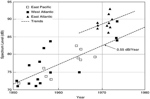
FIGURE 2-7 Long-term trend for low-frequency ambient levels for period 1958– 1975. SOURCE: Ross, 1993, courtesy of Acoustics Bulletin.
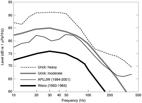
FIGURE 2-8 Point Sur autospectra compared with Wenz (1969). Point Sur data are converted to one-third octave levels and then normalized by the third-octave bandwidths for direct comparison. Shown for reference are the “heavy” and “moderate” shipping average deep-water curves presented by Urick. SOURCE: Andrew et al., 2002. Reprinted with permission of the Acoustical Society of America.
In another attempt to assess long-term trends, Andrew et al. (2002) compared noise measurements made on a receiver on the continental slope of Point Sur, California, from 1994 to 2001 with those collected on the same receiver from 1963 to 1965 (Wenz, 1969). The results of their analysis indicated an increase of approximately 10 dB over 33 years (about 0.3 dB per year) from 20 to 80 Hz (Figure 2-8). Andrew et al. attributed this change principally to increases in the number and gross tonnage of commercial ships, a conclusion consistent with Ross’s results. They indicated that they do not have a satisfactory explanation for the increased noise from 100 to 400 Hz (up to 9 dB) or the minimum increase of 3 dB close to 100 Hz.
Mazzuca (2001) synthesized the results of Ross (1976) and Wenz (1969) to obtain an overall 16-dB increase in low-frequency noise level from shipping during the period 1950-2000. This value corresponds to a rate of increase of 0.32 dB per year, or about 3 dB per decade.
Indicators for Evaluating and Predicting Shipping Noise
How does one quantitatively correlate ocean noise levels with shipping activity and its origins in industrial activities? Efforts to determine the principal sources of noise on ships have constituted an active area of research for quite some time. The classical model, put forward by Ross (1976), states that ship-radiated noise is directly related to ship length and speed. Yet this theory was criticized recently by Wales and Heitmeyer (2002), who contend that there is a “negligible correlation between the source level and the ship speed and the source level and the ship length.” Part of the reason for this lack in correlation may be due to the type of source model used by Wales and Heitmeyer (Heitmeyer, personal communication, 2002). In any case, these observations complicate attempts to determine the principal ship parameters affecting the overall noise levels associated with a large number of ships. Nevertheless, it is possible to make some general well-founded comments regarding ship-radiated noise and shipping traffic and their possible implications for long-term ocean noise levels.
First, there is no doubt that ships generate noise, principally by propeller cavitation and machinery. Second, it is well known that aging ships tend to generate more noise as mechanical and electrical systems deteriorate over time. Third, newer ships have a number of noise-mitigating characteristics, including quieter diesel-electric propulsion systems and deeper propellers that are less prone to cavitation. Fourth, and most important, the number of ships and gross tonnage of the world fleet have increased substantially since 1950 (Figure 2-9) (McCarthy and Miller, 2002). During this period, the number of ships almost tripled (from 30,000 to 87,000 ships), while the gross tonnage increased by a factor of about 6.5 (from 85 to 550 million gross tons). Interestingly, the logarithmic (dB) equivalent of a factor of 6.5 is about 16 dB, exactly corresponding to the observed increase in low-frequency noise levels. These data suggest the following simple relationship between changes in noise levels and gross tonnage:
(2-2)
While Equation 2-2 is highly speculative and its predictive capability must be tested (other parameters, such as changes in ship speed, may need to be included, although they may all be correlated with gross tonnage), there is no doubt that world economic conditions influence shipping activity, which in turn affects overall noise levels in the sea. Westwood et al. (2002) estimate “that over 90 percent of world trade is carried by sea and over the period 1985 to 1999, world seaborne trade increased by 50 percent to
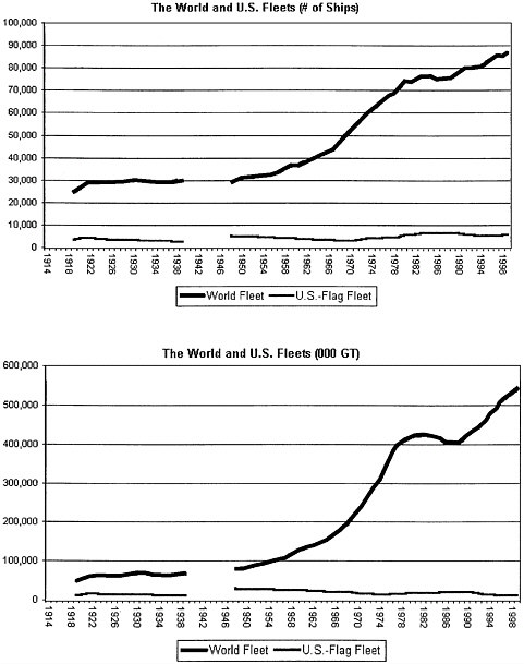
FIGURE 2-9 Global shipping fleet trends, 1914–1998. Only those commercial ships registered in the U.S. (the U.S. flag fleet) are subject to U.S. regulations and laws when operating outside U.S. territorial waters. SOURCE: McCarthy, 2001. Courtesy of http://coultoncompany.com.
about 5 billion tons with the largest increase coming in crude oil and oil products shipments. During 1990-1998 growth averaged 3.2 percent per annum.” The 50 percent trade increase is comparable to the 38 percent increase in gross tonnage during the same period. Applying Equation 2-2 gives a result, 20*log(1.38) = 2.8, which is not much different from the
expected increase in noise levels of 4.5 dB (equal to 0.32 dB/year multiplied by 14 years) for this same time period. Only further study can elucidate whether the similarity in these figures is purely coincidental or scientifically meaningful.
Long-Term Trends in Other Sources of Ocean Noise
No long-term systematic ocean acoustics data set exists to permit a scientific assessment of trends of noise in the ocean. Therefore, the following discussion speculates on possible trends rather than describing any. Although the levels of naturally occurring sound from physical sources (particularly wind-generated and ice-generated noise) may be changing as a result of possible changes in weather patterns associated with global warming, these changes are believed to be dwarfed by other trends. Ocean measurements do exist that demonstrate that ambient sound from some biological sources is increasing in a few locations in the world, for example, sounds produced by humpback whales in the waters around Australia (Cato and McCauley, 2002). The noise associated with whales is expected to asymptote at preexploitation levels as the whale populations return to their preexploitation numbers. However, the overall trend in noise from all biological sources is unknown.
Regarding anthropogenic noise sources, the previous sections of this chapter show that educated speculation (Ross, 1976; Mazzuca, 2001) and measurements at one location (Andrew et al., 2002) suggest that shipping noise at low frequencies (20-80 Hz) has increased by about 10-15 dB over a 25-50-year period. Although the decrease in detection range associated with this increase in noise can be calculated from a sonar systems perspective, the degree to which this change has an adverse impact on the marine environment is unknown. The change in level itself is not a cause of great concern given that naturally occurring processes can change noise levels by 20-30 dB over short periods (e.g., Plate 1). However, other properties of this increase in shipping noise may be biologically important, such as the increase in the prevalence of noise (decrease in time intervals between shipping-noise-dominated periods or increase in the number of locations where shipping noise is a significant contributor), the character of the shipping-generated signals themselves, and so on. Increases in the number and size of commercial and recreational craft have resulted in noise-level increases substantially greater than 10 dB in some areas (e.g., 30 dB or so in the frequency band from 10 to 100 Hz in Singapore Harbor) (Potter and Delory, 1998), but the potential impact on these environments is unknown. This trend has been accompanied by the proliferation of boats and ships equipped with depth sounders and fish finders, which have likely raised the high-frequency (above a few kilohertz) noise in some localized areas. Again, the amount of increase and its potential effects are unknown.
Trends in seismic exploration are much simpler to define in terms of activity than in terms of contribution to the underwater sound field. As discussed previously in this chapter, industry publications periodically report the numbers of surveys presently being conducted in general locations. However, given that exploration methods have been changing, for example, large explosive sources have been replaced by air-guns, which have evolved into air-gun arrays that focus the radiated acoustic energy in the vertical direction, and that undiscovered oil and gas reserves probably are deeper within the earth and/or are to be found in deeper waters, the overall impact of changes on the ocean sound field is difficult to evaluate without a combined ocean noise measurement and numerical modeling effort.
In contrast to focusing of acoustic energy in the vertical by present-day geophysical exploration sources, the newly developing low-frequency navy sonars radiate acoustic energy preferentially in the horizontal direction. Because of the very low absorption of sound in the ocean at low frequencies, these active sonar signals can travel over large distances. Another recent trend in U.S. military sonar has been toward the use of active systems in coastal and shallow-water regions. These sonars have the potential to adversely impact marine mammals; evidence indicates that navy mid-frequency (1-10 kHz) tactical sonars were directly related to the March 2000 mass stranding of marine mammals in the Bahamas (Evans and England, 2001). Other mass strandings have been associated with the transmission of high-level sonar signals, for instance, the May 1996 event in the Mediterranean Sea (D’Amico and Verboom, 1998). Whatever the frequency band, the growth of sonar activity for military purposes started from essentially zero to the present-day levels over just the last half century or so.
The number and type of man-made explosions that affect the world’s oceans also have been changing. The largest of these events is associated with nuclear tests, which have taken place only since 1945 (Lawson, 2002). Many of the early tests by the United States from 1945 to 1962 were atmospheric tests conducted on small islands in the central part of the Pacific Ocean just north of the equator. The energy released during these tests certainly created high-level impulsive ocean acoustic signals that traveled over great distances. Much of the subsequent U.S. testing was done underground, sufficiently far from the coast that little impact on the ocean environment occurred. However, underground tests near coastlines can create high levels of underwater sound. As an illustration, one of the French nuclear tests in 1995-1996 on the Mururoa Atoll in French Polynesia in the South Pacific Ocean generated underwater signals that were recorded by a single omnidirectional hydrophone at a range of 6,670 km with levels 20-45 dB above background noise across the frequency band 2-30 Hz (D’Spain et al., 2001). Given the steady progress since the mid-1990s in the number of nations that have signed, and have ratified, the Comprehensive Nuclear Test Ban Treaty, these tests appear to be increasingly rare.
Long-term trends in the use of chemical explosive devices also may be taking place. Any speculation on these trends must exclude times of war (the underwater noise created by explosions during the great naval battles in World War II must have been extremely high) since the occurrence of war and resulting contributions to the ocean noise field are highly unpredictable and extremely episodic. Long-term trends in the use of smaller explosive devices also may be taking place. As mentioned previously, explosive sources used in seismic exploration are being replaced by air-gun arrays. However, explosives are routinely used to sever abandoned well-heads so that they can be removed and to decommission the rigs themselves. As oil production in a given region matures and declines, the use of explosives in this way increases. The use of explosives in ocean acoustic and geophysical research has decreased, but these sources still are deployed in a few experiments. Military use of explosive charges as the source component in active sonar systems (e.g., SUS; Urick, 1975) appears to be decreasing. Hull shock tests are rare events and do not appear to be changing significantly in frequency of occurrence. The use of seal bombs has been discouraged by U.S. and international regulations and is being replaced by other types of acoustic deterrent devices. Fishing by the detonation of underwater explosives (a technique whose success improves with its increasing adverse impact on the marine environment) is banned but still is practiced in some regions. In any case, one quantitative measure of the long-term change in numbers and spatial distribution of underwater explosions is possible to obtain, at least for the North Pacific Ocean. The number and estimated source locations of detonations recorded over a modern-day period of time could be compared to those recorded by 20 Missile Impact Location System hydrophones over a one-year period from August 1965 to July 1966 (following Spiess et al., 1968). Nearly 20,000 explosions were detected within this one-year period, with the winter rate of occurrence of 300 explosions per month increasing to 4,000 explosions per month in summer. The highest activity was detected off the west coast of North America, in the Gulf of Alaska, north of Hawaii, and seaward of the Japanese and Kuril Islands (Spiess et al., 1968). The significance of any of these possible changes in the occurrence of underwater explosions to the marine environment is unknown.


