
F
Simulating False Match Probabilities Based on Normal Theory1
WHY THE FALSE MATCH PROBABILITY DEPENDS ON ONLY RATIO δ / σ
As a function of δ, we are interesed in P{match on one element is declared | |µx − µy| > δ}, where µx and µy are the true means of one of the seven elements in the melts of the CS and PS bullets, respectively. The within-replicate variance is generally small, so we assume that the sample means of the three replicates are normally distributed; that is,
where “~” stands for “is distributed as.” Thus, the difference in the means is δ. We further assume that the errors in the measurements leading to ![]() and
and ![]() are independent. Based on this specification (or “these assumptions”), statistical theory asserts that
are independent. Based on this specification (or “these assumptions”), statistical theory asserts that
where ![]() and
and ![]() denotes the chi-squared distribution on four degrees of freedom. If σ2 is estimated from a pooled variance on B (more than 2) samples, then
denotes the chi-squared distribution on four degrees of freedom. If σ2 is estimated from a pooled variance on B (more than 2) samples, then ![]() Let v equal the number of degrees of freedom used to estimate σ, for example, v = 4 if
Let v equal the number of degrees of freedom used to estimate σ, for example, v = 4 if ![]()
…+ s2B)/B. The ratio of ![]() to
to ![]() is the same as the distribution of
is the same as the distribution of ![]() namely a Student’s tv (v degrees of freedom), so the two-sample t statistic is distributed as a (central) Student’s t on v degrees of freedom:
namely a Student’s tv (v degrees of freedom), so the two-sample t statistic is distributed as a (central) Student’s t on v degrees of freedom:
The FBI criterion for a match on this one element can be written
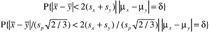
Because E(sx) = E(sy) = 0.8812σ, and E(sp) ≈ σ if v > 60, this reduces very roughly to
The approximation is very rough because E(P{t < S}) ≠ P{t < E(S)}, where t stands for the two-sample t statistic and S stands for ![]() But it does show that if δ is very large, this probability is virtually zero (very small false match probability because the probability that the sample means would, by chance, end up very close together is very small). However, if δ is small, the probability is quite close to 1.
But it does show that if δ is very large, this probability is virtually zero (very small false match probability because the probability that the sample means would, by chance, end up very close together is very small). However, if δ is small, the probability is quite close to 1.
The equivalence t test proceeds as follows. Assume
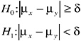
where H0 is the null hypothesis that the true population means differ by at least δ, and the alternative hypothesis is that they are within δ of each other. The two-sample t test would reject H0 in favor of H1 if the sample means are too close, that is, if ![]() where Kα(n,δ) is chosen so that
where Kα(n,δ) is chosen so that ![]() does not exceed a preset per-element risk level of α (in Chapter 3, we used α = 0.30). Rewriting that equation, and writing Kα for Kα(n,δ),
does not exceed a preset per-element risk level of α (in Chapter 3, we used α = 0.30). Rewriting that equation, and writing Kα for Kα(n,δ),
When v is large sp ≈ 0, and therefore the quantity ![]()
That shows that the false match probability depends on δ and σ only through the ratio. (The argument is a little more complicated when v is small, because the ratio ![]() is a random quantity, but the conclusion will be the same.) Also, when v is large, the quantity
is a random quantity, but the conclusion will be the same.) Also, when v is large, the quantity ![]() which is distributed as a standard normal distribution. So the probability can be written
which is distributed as a standard normal distribution. So the probability can be written
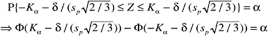
where Φ(·) denotes the standard cumulative normal distribution function (for example, Φ(1.645) = 0.95). So, for large values of v, the nonlinear equation can be solved for Kα, so that the probability of interest does not exceed α. For small values of v, Kα is the 100(1 − α)% point of the non-central t distribution with v degrees of freedom and noncentrality parameter ![]() (Ref. 14).
(Ref. 14).
Values of Kα are given in Table F.1 below, for various values of α (0.30, 0.25, 0.20, 0.10, 0.05, 0.01, and 0.0004), degrees of freedom (4, 40, 100, and 200), and δ / σ (0.25, 0.33, 0.50, 1, 1.5, 2, and 3). The theory for Hotelling’s T2
TABLE F.1 Values of Kα(n,v) Used in Equivalence t Test (Need to Multiply by ![]()
|
α = 0.30, n = 3 |
|||||||
|
(δ / σ) |
|||||||
|
|
0.25 |
0.33 |
0.50 |
1 |
1.5 |
2 |
3 |
|
v = 4 |
0.43397 |
0.44918 |
0.49809 |
0.81095 |
1.35161 |
1.94726 |
3.12279 |
|
40 |
0.40683 |
0.42113 |
0.46725 |
0.77043 |
1.31802 |
1.92530 |
3.13875 |
|
100 |
0.40495 |
0.41919 |
0.46511 |
0.76783 |
1.31622 |
1.92511 |
3.14500 |
|
200 |
0.40435 |
0.41857 |
0.46443 |
0.76697 |
1.31563 |
1.92510 |
3.14734 |
|
α = 0.30, n = 5 |
||||||
|
(δ / σ) |
||||||
|
|
0.25 |
0.33 |
0.50 |
1 |
2 |
3 |
|
v = 4 |
0.44761 |
0.47385 |
0.56076 |
1.11014 |
2.63496 |
4.12933 |
|
40 |
0.41965 |
0.44436 |
0.52681 |
1.07231 |
2.63226 |
4.19067 |
|
100 |
0.41771 |
0.44232 |
0.52445 |
1.06984 |
2.63546 |
4.20685 |
|
200 |
0.41710 |
0.44167 |
0.52370 |
1.06906 |
2.63664 |
4.21278 |
|
α = 0.25, n = 3 |
|||||||
|
(δ / σ) |
|||||||
|
|
0.25 |
0.33 |
0.50 |
1 |
1.5 |
2 |
3 |
|
v = 4 |
0.35772 |
0.37030 |
0.41092 |
0.68143 |
1.19242 |
1.77413 |
2.91548 |
|
40 |
0.33633 |
0.34818 |
0.38655 |
0.64811 |
1.16900 |
1.77305 |
2.98156 |
|
100 |
0.33484 |
0.34664 |
0.38484 |
0.64578 |
1.16765 |
1.77420 |
2.99223 |
|
200 |
0.33437 |
0.34615 |
0.38430 |
0.64503 |
1.16722 |
1.77461 |
2.99595 |
|
α = 0.25, n = 5 |
|||||||
|
(δ / σ) |
|||||||
|
|
0.25 |
0.33 |
0.50 |
1 |
1.5 |
2 |
3 |
|
v = 4 |
0.36900 |
0.39075 |
0.46350 |
0.95953 |
1.70024 |
2.44328 |
3.88533 |
|
40 |
0.34696 |
0.36748 |
0.43648 |
0.92903 |
1.69596 |
2.47772 |
4.02810 |
|
100 |
0.34542 |
0.36586 |
0.43459 |
0.92698 |
1.69672 |
2.48365 |
4.05178 |
|
200 |
0.34493 |
0.36534 |
0.43399 |
0.92633 |
1.69700 |
2.48570 |
4.06021 |
|
α = 0.222, n = 3 |
|||||||
|
(δ / σ) |
|||||||
|
|
0.25 |
0.33 |
0.50 |
1 |
1.5 |
2 |
3 |
|
4 |
0.31603 |
0.32716 |
0.36318 |
0.60827 |
1.09914 |
1.67316 |
2.79619 |
|
40 |
0.29754 |
0.30804 |
0.34207 |
0.57848 |
1.07949 |
1.68119 |
2.88735 |
|
100 |
0.29625 |
0.30670 |
0.34060 |
0.57638 |
1.07834 |
1.68290 |
2.90000 |
|
200 |
0.29584 |
0.30627 |
0.34013 |
0.57571 |
1.07798 |
1.68350 |
2.90436 |
|
α = 0.222, n = 5 |
|||||||
|
(δ / σ) |
|||||||
|
|
0.25 |
0.33 |
0.50 |
1 |
1.5 |
2 |
3 |
|
3 |
0.32601 |
0.34528 |
0.41003 |
0.87198 |
1.60019 |
2.33249 |
3.74571 |
|
40 |
0.30695 |
0.32514 |
0.38655 |
0.84440 |
1.60422 |
2.38467 |
3.93060 |
|
100 |
0.30562 |
0.32374 |
0.38490 |
0.84252 |
1.60548 |
2.39187 |
3.95822 |
|
200 |
0.30520 |
0.32329 |
0.38438 |
0.84192 |
1.60592 |
2.39434 |
3.96795 |
|
(δ / σ) |
||||||
|
|
0.25 |
0.33 |
0.50 |
1 |
2 |
3 |
|
v = 4 |
0.28370 |
0.29370 |
0.32612 |
0.55032 |
1.59066 |
2.69968 |
|
40 |
0.26736 |
0.27680 |
0.30744 |
0.52321 |
1.60451 |
2.80887 |
|
100 |
0.26622 |
0.27561 |
0.30613 |
0.52129 |
1.60656 |
2.82294 |
|
200 |
0.26585 |
0.27523 |
0.30571 |
0.52068 |
1.60725 |
2.82774 |
|
α = 0.20, n = 5 |
||||||
|
(δ / σ) |
||||||
|
|
0.25 |
0.33 |
0.50 |
1 |
2 |
3 |
|
v = 4 |
0.29266 |
0.30999 |
0.36844 |
0.80094 |
2.24256 |
3.63322 |
|
40 |
0.27582 |
0.29219 |
0.34759 |
0.77521 |
2.30710 |
3.84954 |
|
100 |
0.27464 |
0.29094 |
0.34612 |
0.77341 |
2.31517 |
3.88010 |
|
200 |
0.27426 |
0.29054 |
0.34566 |
0.77285 |
2.31790 |
3.89081 |
|
α = 0.10, n = 3 |
||||||
|
(δ / σ) |
||||||
|
|
0.25 |
0.33 |
0.50 |
1 |
2 |
3 |
|
v = 4 |
0.14025 |
0.14521 |
0.16138 |
0.28009 |
1.14311 |
2.19312 |
|
40 |
0.13257 |
0.13726 |
0.15256 |
0.26552 |
1.16523 |
2.36203 |
|
100 |
0.13203 |
0.13670 |
0.15193 |
0.26449 |
1.16738 |
2.38036 |
|
200 |
0.13186 |
0.13653 |
0.15174 |
0.26416 |
1.16808 |
2.38652 |
|
α = 0.10, n = 5 |
||||||
|
(δ / σ) |
||||||
|
|
0.25 |
0.33 |
0.50 |
1 |
2 |
3 |
|
v = 4 |
0.14470 |
0.15332 |
0.18272 |
0.44037 |
1.76516 |
3.05121 |
|
40 |
0.13678 |
0.14493 |
0.17277 |
0.42178 |
1.86406 |
3.39055 |
|
100 |
0.13622 |
0.14434 |
0.17207 |
0.42044 |
1.87408 |
3.43264 |
|
200 |
0.13604 |
0.14416 |
0.17184 |
0.42001 |
1.87741 |
3.44712 |
|
α = 0.05, n = 3 |
||||||
|
(δ / σ) |
||||||
|
|
0.25 |
0.33 |
0.50 |
1 |
2 |
3 |
|
4 |
0.07000 |
0.07241 |
0.08048 |
0.14085 |
0.80000 |
1.82564 |
|
40 |
0.06614 |
0.06847 |
0.07612 |
0.13329 |
0.80877 |
2.00110 |
|
100 |
0.06580 |
0.06812 |
0.07584 |
0.13280 |
0.80951 |
2.01774 |
|
200 |
0.06588 |
0.06822 |
0.07573 |
0.13263 |
0.80976 |
2.02351 |
|
α = 0.05, n = 5 |
||||||
|
(δ / σ) |
||||||
|
|
0.25 |
0.33 |
0.50 |
1 |
2 |
3 |
|
4 |
0.07215 |
0.07645 |
0.09118 |
0.22900 |
1.41106 |
2.64066 |
|
40 |
0.06825 |
0.07232 |
0.08626 |
0.21748 |
1.50372 |
3.02532 |
|
100 |
0.06798 |
0.07203 |
0.08591 |
0.21672 |
1.51184 |
3.06786 |
|
200 |
0.06789 |
0.07194 |
0.08580 |
0.21647 |
1.51462 |
3.08296 |
|
α = 0.01, n = 3 |
||||||
|
(δ / σ) |
||||||
|
|
0.25 |
0.33 |
0.50 |
1 |
2 |
3 |
|
4 |
0.01397 |
0.01447 |
0.01608 |
0.02823 |
0.25124 |
1.21164 |
|
40 |
0.01322 |
0.01369 |
0.01522 |
0.02671 |
0.24129 |
1.33049 |
|
100 |
0.01317 |
0.01364 |
0.01516 |
0.02660 |
0.24062 |
1.34080 |
|
200 |
0.01315 |
0.01352 |
0.01514 |
0.02656 |
0.24040 |
1.34432 |
|
α = 0.01, n = 5 |
||||||
|
(δ / σ) |
||||||
|
|
0.25 |
0.33 |
0.50 |
1 |
2 |
3 |
|
4 |
0.01442 |
0.01528 |
0.01823 |
0.04651 |
0.79664 |
1.98837 |
|
40 |
0.01364 |
0.01446 |
0.01724 |
0.04400 |
0.83240 |
2.35173 |
|
100 |
0.01359 |
0.01440 |
0.01717 |
0.04383 |
0.83521 |
2.38989 |
|
200 |
0.01357 |
0.01438 |
0.01715 |
0.04378 |
0.83616 |
2.40330 |
|
α = 0.0004, n = 3 |
|||||||
|
(δ / σ) |
|||||||
|
|
0.25 |
0.33 |
0.50 |
1 |
2 |
3 |
4.4 |
|
4 |
0.00056 |
0.00058 |
0.00064 |
0.00113 |
0.01071 |
0.34213 |
1.5877 |
|
40 |
0.00053 |
0.00055 |
0.00061 |
0.00107 |
0.01013 |
0.34139 |
1.9668 |
|
100 |
0.00053 |
0.00055 |
0.00061 |
0.00107 |
0.01009 |
0.34133 |
2.0072 |
|
200 |
0.00053 |
0.00055 |
0.00060 |
0.00106 |
0.01008 |
0.34131 |
2.0215 |
is similar (it uses vectors and matrices instead of scalars), and the resulting critical value comes from a noncentral F distribution (Ref. 15).2
ESTIMATING MEASUREMENT UNCERTAINTY WITH POOLED STANDARD DEVIATIONS
Chapter 3 states that a pooled estimate of the measurement uncertainty σ, sp, is more accurate and precise than an estimate based on only sx, the sample SD based on only three normally distributed measurements. That statement follows from the fact that a squared sample SD has a chi-squared distribution; specifically, (n − 1)s2 / σ2 has a chi-squared distribution on (n − 1) degrees of freedom, where s is based on n observations. The mean of the square root of a chi-squared random variable based on v = (n − 1) degrees of freedom is ![]() where Γ(·) is the gamma function. For v = (n − 1) = 2, E(s) = 0.8812σ; for v = 4 (i.e., estimating σ by
where Γ(·) is the gamma function. For v = (n − 1) = 2, E(s) = 0.8812σ; for v = 4 (i.e., estimating σ by ![]() E(s) = 0.9400σ; for v = 200 (that is, estimating σ by the square root of the mean of the squared SDs from 100 bullets), E(s) ≈ σ. In addition, the probability that s exceeds 1.25σ when n = 2 (that is, using only one bullet) is 0.21 but falls to 0.00028 when v = 200. For those
E(s) = 0.9400σ; for v = 200 (that is, estimating σ by the square root of the mean of the squared SDs from 100 bullets), E(s) ≈ σ. In addition, the probability that s exceeds 1.25σ when n = 2 (that is, using only one bullet) is 0.21 but falls to 0.00028 when v = 200. For those
|
2 |
These values were determined by using a simple binary search algorithm for the value α and the R function pf(x, 1, dof, 0.5*n*E), where n = 3 or 5 and E = (δ / σ)2. R is a statistical-analysis software program that is downloadable from http://www.r-project.org. |
reasons, sp based on many bullets is preferable to estimating σ by using only three measurements on a single bullet.
WITHIN-BULLET VARIANCES, COVARIANCES, AND CORRELATIONS FOR FEDERAL BULLET DATA SET
The data on the Federal bullets contained measurements on six of the seven elements (all but Cd) with ICP-OES. They allowed estimation of within-bullet variances, covariances, and correlations among the six elements. According to the formula in Appendix K, now applied to the six elements, the estimated within-bullet variance matrix is given below. The correlation matrix is found in the usual way (for example, Cor (Ag, Sb) = Covariance(Ag,Sb)/[SD(Ag) SD(Sb)]. Covariances and correlations between Cd and all other elements are assumed to be zero. The correlation matrix was used to demonstrate the use of the equivalence Hotelling’s T2 test. Because it is based on 200 bullets measured in 1991, it is presented here for illustrative purposes only.
|
Within-Bullet Variances and Covariances ×105, log(Federal Data) |
||||||
|
|
ICP-As |
ICP-Sb |
ICP-Sn |
ICP-Bi |
ICP-Cu |
ICP-Ag |
|
ICP-As |
187 |
27 |
31 |
31 |
37 |
77 |
|
ICP-Sb |
20 |
37 |
25 |
18 |
25 |
39 |
|
ICP-Sn |
31 |
25 |
106 |
16 |
29 |
41 |
|
ICP-Bi |
31 |
18 |
16 |
90 |
14 |
44 |
|
ICP-Cu |
37 |
25 |
29 |
14 |
40 |
42 |
|
ICP-Ag |
77 |
39 |
41 |
44 |
42 |
681 |
|
Within-Bullet Correlations, Federal Data |
|||||||
|
|
ICP-As |
ICP-Sb |
ICP-Sn |
ICP-Bi |
ICP-Cu |
ICP-Ag |
(Cd) |
|
ICP-As |
1.000 |
0.320 |
0.222 |
0.236 |
0.420 |
0.215 |
0.000 |
|
ICP-Sb |
0.320 |
1.000 |
0.390 |
0.304 |
0.635 |
0.242 |
0.000 |
|
ICP-Sn |
0.222 |
0.390 |
1.000 |
0.163 |
0.440 |
0.154 |
0.000 |
|
ICP-Bi |
0.236 |
0.304 |
0.163 |
1.000 |
0.240 |
0.179 |
0.000 |
|
ICP-Cu |
0.420 |
0.635 |
0.440 |
0.240 |
1.000 |
0.251 |
0.000 |
|
ICP-Ag |
0.215 |
0.242 |
0.154 |
0.179 |
0.251 |
1.000 |
0.000 |
|
(Cd) |
0.000 |
0.000 |
0.000 |
0.000 |
0.000 |
0.000 |
1.000 |
BETWEEN-ELEMENT CORRELATIONS
In Chapter 3, correlations between mean concentrations of bullets were estimated by using the Pearson correlation coefficient (see equation 2). One reviewer suggested that Spearman’s rank correlation may be more appropriate, as it provides a nonparametric estimate of the monotonic association between two variables. Spearman’s rank correlation coefficient takes the same form as Equation 2, but with the ranks of the values (numbers 1, 2, 3, …, n = number of data
pairs) rather than values themselves. The table below consists of 49 entries, corresponding to all possible pairs of the seven elements. The value 1.000 on the diagonal confirms a correlation of 1.000 for an element with itself. The values in the cells on either side of the diagonal are the same because the correlation between, say, As and Sb is the same as that between Sb and As. For these off-diagonal cells, the first line reflects the conventional Pearson correlation coefficient based on the 1,373-bullet subset from the 1,837-bullet subset (bullets with all seven measured elements or with six measured and one imputed for Cd). The second line is Spearman’s rank correlation coefficient on rank(data), again for
|
|
As |
Sb |
Sn |
Bi |
Cu |
Ag |
Cd |
|
As |
1.000 |
0.556 |
0.624 |
0.148 |
0.388 |
0.186 |
0.242 |
|
|
|
0.697 |
0.666 |
0.165 |
0.386 |
0.211 |
0.166 |
|
|
|
0.678 |
0.667 |
0.178 |
0.392 |
0.216 |
0.279 |
|
|
|
1750 |
1,381 |
1742 |
1,743 |
1,750 |
856 |
|
Sb |
0.556 |
1.000 |
0.455 |
0.157 |
0.358 |
0.180 |
0.132 |
|
|
0.697 |
|
0.556 |
0.058 |
0.241 |
0.194 |
0.081 |
|
|
0.678 |
|
0.560 |
0.054 |
0.233 |
0.190 |
0.173 |
|
|
1,750 |
|
1,387 |
1829 |
1,826 |
1,837 |
857 |
|
Sn |
0.624 |
0.455 |
1.000 |
0.176 |
0.200 |
0.258 |
0.178 |
|
|
0.666 |
0.556 |
|
0.153 |
0.207 |
0.168 |
0.218 |
|
|
0.667 |
0.560 |
|
0.152 |
0.208 |
0.165 |
0.385 |
|
|
1,381 |
1,387 |
|
1385 |
1380 |
1387 |
857 |
|
Bi |
0.148 |
0.157 |
0.176 |
1.000 |
0.116 |
0.560 |
0.030 |
|
|
0.165 |
0.058 |
0.153 |
|
0.081 |
0.499 |
0.103 |
|
|
0.178 |
0.054 |
0.152 |
|
0.099 |
0.522 |
0.165 |
|
|
1,742 |
1,829 |
1,385 |
|
1,818 |
1,829 |
857 |
|
Cu |
0.388 |
0.358 |
0.200 |
0.116 |
1.000 |
0.258 |
0.111 |
|
|
0.386 |
0.241 |
0.207 |
0.081 |
|
0.206 |
0.151 |
|
|
0.392 |
0.233 |
0.208 |
0.099 |
|
0.260 |
0.115 |
|
|
1,743 |
1,826 |
1,380 |
1818 |
|
1826 |
855 |
|
Ag |
0.186 |
0.180 |
0.258 |
0.560 |
0.258 |
1.000 |
0.077 |
|
|
0.211 |
0.194 |
0.168 |
0.499 |
0.206 |
|
0.063 |
|
|
0.216 |
0.190 |
0.165 |
0.522 |
0.260 |
|
0.115 |
|
|
1,750 |
1,837 |
1,387 |
1829 |
1,826 |
|
857 |
|
Cd |
0.242 |
0.132 |
0.178 |
0.030 |
0.111 |
0.077 |
1.000 |
|
|
0.166 |
0.081 |
0.218 |
0.103 |
0.151 |
0.063 |
|
|
|
0.279 |
0.173 |
0.385 |
0.165 |
0.251 |
0.115 |
|
|
|
857 |
857 |
857 |
857 |
855 |
857 |
|
the 1,373-bullet subset. The third line is Spearman’s rank correlation coefficient on the entire 1,837-bullet subset (some bullets had only three, four, five, or six elements measured). The fourth line gives the number of pairs in Spearman’s rank correlation coefficient calculation. All three sets of correlation coefficients are highly consistent with each other. Regardless of the method used to estimate the linear association between elements, associations between As and Sb, between As and Sn, between Sb and Sn, and between Ag and Bi are rather high. Because the 1,837-bullet subset is not a random sample from any population, we refrain from stating a level of “significance” for these values, noting only that regardless of the method used to estimate the linear association between elements, associations between As and Sb, between As and Sn, between Sb and Sn, and between Ag and Bi are higher than those for the other 17 pairs of elements.


