
3
Spatial Thinking in Everyday Life, at Work, and in Science
3.1 INTRODUCTION
Literacy in the classically linguistic sense means that someone can read, write, and speak in a language. Those abilities can be seen in all aspects of our existence: in spoken and written communications in everyday life, in the workplace, and in science. Spatial literacy follows a similar pattern: people draw upon their spatial knowledge, their repertoire of spatial ways of thinking and acting, and their spatial capabilities to solve problems in all aspects of their lives.
Section 3.2 explores the ways in which spatial thinking underpins activities that range across the fabric of our everyday lives. For the vast majority of these activities, there is no formal instruction in how to use spatial thinking to solve problems. This lack of formal instruction is in direct contrast to the formal learning that enables the use of spatial thinking in the workplace and science. Section 3.3 illustrates how novices and experts in various crafts and professions use spatial thinking skills in their work. Section 3.4 introduces the fundamental link between doing science and thinking spatially, explaining the parallels among the three disciplines—astronomy, geoscience, and geography—that are the basis for four case studies. The case studies illustrate a set of themes: the role of spatial thinking in historical changes in our most fundamental understandings of the physical world (Section 3.5 on spatial thinking in astronomy), the challenges of learning the component operations of spatial thinking during the novice-to-expert transition in a discipline (Section 3.6 on learning to think spatially in the geosciences), and the role of particularly gifted spatial thinkers in shaping understanding in a discipline (Section 3.7 on Marie Tharp in geoscience and Section 3.8 on Walter Christaller in geography).
3.2 SPATIAL THINKING IN EVERYDAY LIFE
In March 2003, Mark Wegner and Deborah Girasek published a study in Pediatrics on the readability of printed instructions for car safety seat (CSS) installation. They were motivated by a report that 79 to 94 percent of child safety seats were improperly installed, while 46 percent of accident-related deaths among children aged 1 to 14 resulted from motor vehicle collisions.
Our data indicate that CSS instructions in the United States are currently written at a reading level that is too high. Experts in the arena of health literacy recommend that materials be targeted to the fifth- or sixth-grade reading level…. The average readability level of the instruction sets that we tested was 10th grade. Researchers … found that approximately two thirds of parents tested in an outpatient clinic could not read at more than a ninth-grade level…. Because parents would be expected to be the main target for CSS instruction sets, this lends additional evidence that the instruction sets may not be reaching the people most likely to benefit from the message. (Wegner and Girasek, 2003, p. 590)
On the face of it, the study confirms general beliefs about the failure of American education to produce verbally literate people who can read polysyllabic words; the authors used the SMOG (Simple Measure of Gobbledygook) statistic based on the number of three or more syllable words in text samples. They recommended that “manufacturers of CSS rewrite their instruction sets to a fifth-grade reading level. This could be accomplished by using shorter sentences and simpler words” (Wegner and Girasek, 2003, p. 591).
In the committee’s judgment, a second message can be drawn. Wegner and Girasek (2003, p. 590) noted that “[t]his study did not take into account some factors that tend to increase comprehensibility, such as the use of illustrations and empty space …” because “… [p]ictures and diagrams were not considered, neither were captions that stood apart from the rest of the instruction set and applied only to pictures” (Wegner and Girasek, 2003, p. 589).
That many car safety seats are improperly installed should come as no surprise to any adult American. The problem is not simply one of comprehension as a function of word complexity, sentence length, and therefore, verbal literacy. Comprehension is a function of another form of literacy, one that is equally essential but largely overlooked. Spatial literacy lies at the heart of spatial thinking. It was unfortunate that Wegner and Girasek chose not to include the pictures and diagrams because installation instructions are a complex combination of text and graphics.
For anyone who has attempted to assemble a child’s bicycle, a piece of furniture, a stereo system, or a ceiling fan (Figure 3.1), the challenge of language is only part of the problem. Instructions control actions. Words have referents, physical objects, and those referents must be correctly identified, aligned, and brought together. Directions such as up and down, front and back, on top of and behind, and left and right become crucial in establishing relations between parts. Parts must be linked into a working whole. Motions involving clockwise versus counterclockwise turns, through versus over versus under, and push versus pull must be distinguished. The coordination among text, schematic diagram, and required actions is critical to success in the assembly process.
Spatial thinking is so deeply embedded in the activities of daily life and thought that it is difficult to disentangle and appreciate its role. We may not even realize its role, but it is fundamental to many taken-for-granted activities, underpinning their successful performance and sometimes accounting for their spectacular failure. Imagine, therefore, a classic middle-class family with two parents and children of various ages. Imagine a typical day in the life of that family. Imagine solving the problems of everyday life.
A phone call in late August to a daughter on a study-abroad program in Europe requires, among other things, working out the right time to call. This requires an understanding of time zones and the use of daylight saving time. A trip to take a son to college involves packing things into boxes and packing boxes into a car trunk and back seat in the most efficient way such that space use is maximized, nothing gets crushed or broken, and things are easy to remove. Getting to the college town and apartment building involves using a web-based search engine to print a route map, and then following written and map directions. The exercise machine that was disassembled and packed has to be reassembled without, unfortunately, the instructions, which have been lost. The now-assembled bunk bed, desk, and shelves have to be fitted into the room without blocking heating vents, electrical outlets, telephone outlets, and the passage to the window, closet, and door in the

FIGURE 3.1 A set of instructions for installing a ceiling fan. Note the appeal to common sense and caution.
apartment. A trip to a supermarket to stock up on food for the refrigerator requires getting verbal driving directions from a neighbor, remembering and following them, and finding where things are located in a store that is organized in ways subtly different from the one that the family is used to. A written grocery list has to be mapped onto the floor plan of the supermarket in an efficient way. To amuse a younger child on the journey home, someone has to help her to put together pieces of a complex jigsaw puzzle. The journey home is complicated by the need to make a detour around construction that was not marked on the downloaded route map. It is also complicated by a flat tire: replacing it with the spare requires understanding the instructions on the side of the jack, removing the bolts and the wheel, and then tightening the bolts in the correct direction and sequence. Returning home, another son is asked to take over lawn mowing duties and has to find an efficient way to maneuver around flower beds and trees in the garden. The youngest child’s shoelace has come undone and there is yet another lesson in how to tie a shoelace properly, a double knot this time. The costume for the middle daughter’s school play has to be cut from fabric, fitted, and sewn by tomorrow’s dress rehearsal.
Everyday life is impregnated with tasks that, on the surface, are routine and trivial. Viewed as problems requiring solutions, these tasks are far from trivial in nature. All of the tasks involve the
concept of space in general and various spaces in particular: global time-space, car trunk space, neighborhood space, supermarket space, room space, machine space, puzzle space, garden space, the space of shoelaces, and the space of dress patterns. Many of the tasks involve graphic representations: the time zone diagram in the telephone directory, the web search engine map, the floor plan of the supermarket, the grocery list, the picture of the completed jigsaw puzzle, and the dress pattern. All tasks involve complex sequences of operations: finding the clock times of the two places and subtracting the right one to work out the time difference; choosing boxes of the right size for the space available, orienting and rotating them, and stacking them; rotating parts, twisting parts, and tightening fastenings; breaking an operation into discrete parts and demonstrating and explaining the operations; making a loop with one lace, putting the other part of the shoe lace over the top of the loop, and so forth. Some of the tasks can be taught formally, such as map reading, whereas others, such as dress making, are no longer taught formally in schools, and still others, such as tying shoelaces, are learned informally as part of everyday life. There is transfer of learning from one task to another; jigsaw puzzles and exercise machine assembly have things in common.
Tasks can be performed in different ways. The web search engine offers three different representations: lists of text instructions, maps with straight-line segments, and conventional road maps. Strategies for solving jigsaw puzzles differ: some people sort straight edge pieces first, then match by shape. Others use color and patterns to make decisions. Some performance differences are significant and lead to faster and more efficient solutions: others, especially shoelace tying styles, are matters of preference (single versus double knots). There are differences based on age and sex in solving problems. Some people approach the trunk-packing task analytically, gauging the dimensions of boxes and thinking about alternative arrangements; others plunge ahead, using trial and error. For many activities, we are not consciously aware of spatial thinking; in other instances, the challenge is explicit and we monitor our own process.
3.3 SPATIAL THINKING AT WORK
Spatial thinking at work begins before work, during the daily challenge of commuting. Many drivers simplify the complex two-dimensional plane between home and work to a line that contains a sequence of turns at landmarks. The rest of the environmental context is not relevant to the task of commuting and therefore is largely ignored during the commute. The path, specifying where to turn and which direction to take, is crucial. As a consequence, people pay more attention to landmarks that mark changes in direction, and they remember those landmarks better than other places along the route (Tom and Denis, 2004).
The cognitive importance of landmarks and turns is reflected in neurophysiology. Using brain imaging technology, researchers have shown connections between cognitive processes and brain functioning (Aguirre et al., 1998; Maguire et al., 1997). There is a greater neurophysiological response to landmarks signaling turns than to landmarks that are simply en route in those areas of the brain underpinning the construction of mental maps (Janzen and van Turennout, 2003). These areas of the brain are larger in people who are expert at navigation, such as London taxi drivers who undergo considerable training before they are allowed to pursue their profession. Neurophysiological findings suggest that extensive spatial experience may lead to physical changes in the brain that may, in turn, further enhance spatial thinking.
Experienced taxi drivers have more extensive and detailed mental maps of the areas they service than do ordinary residents. Nevertheless, taxi drivers’ mental maps are simplified in the same ways as those of regular commuters. For example, taxi drivers think about the main arteries of a city as being straighter and more aligned with cardinal directions than they actually are. This illustrates an important characteristic of expertise. Expertise draws on the same mechanisms as
normal, everyday cognitive processing; the novice-expert difference is a consequence of the degree and type of practice and experience in a domain.
Getting to work is not the only spatial task shared by different occupations. In order to operate, workers need a mental model of the structure and functioning of the institution: they need to know who to turn to for help on what task. Sometimes information is mentally represented as a spatial network, much like a rudimentary mental map of an environment. In this institutional mental space, links are tasks and nodes are people who perform tasks. Often information is explicitly represented in an organizational chart and depicted as a spatial network that must be “navigated.” Managers must decide how to allocate resources or what new projects to undertake. To do so, they consult charts and graphs of performance. Charts and graphs provide spatial representations of data, but do not in themselves provide solutions to problems. Solutions depend on making inferences from charts and graphs, projections of future sales, changes in personnel and equipment, and more.
Beyond generic problem-solving similarities, many jobs require the use of specific spatial skills. Recognition of complex patterns is required in many professions. Think of the time you saw an X-ray image in a doctor’s office. You could probably pick out bones but little else. In the clouds that X-rays resemble, highly trained radiologists can discern tumors, blood clots, and faulty valves. Recognizing these patterns takes years of training and is by no means perfect (see Ericsson, 1996, for an overview of the literature on expertise; see the November 2003 issue of the Educational Researcher on expertise in the context of education).
Recognition skill does not transfer to other domains. Skilled radiologists are no better than novices at recognizing skin diseases that dermatologists are expert in diagnosing or plant diseases that botanists excel at discerning. Expertise in pattern recognition is domain specific. It requires discerning features characteristic of specific sensory categories. Typically, domain expertise in pattern recognition also requires learning the proper configurations of distinctive features. The practice that polishes this skill requires categorizing many examples of related and different phenomena and getting feedback on the categorization process. Simply seeing examples is not sufficient; to become expert, people must learn to differentiate and discriminate one category from another (Nickerson and Adams, 1979). A classroom demonstration illustrates that seeing, however frequent, is insufficient to ensure learning critical features. Students are asked to name what is shown on both sides of a penny or whether their (analog) watch dial has lines or numbers to mark minutes. Few succeed at the penny task, and many are surprisingly poor at the watch task. Although we “look” at pennies and watches frequently, often many times a day, we do not have to distinguish one penny or watch face from another (Nickerson and Adams, 1979). We do, however, need to distinguish a penny from a nickel or dime, and we do so based on color or shape or size without paying attention to the face of the coin. In watches, we only consult the lengths of hands and their angles. When we need to make fine distinctions, such as those required to differentiating types of tumors or diagnosing skin diseases, we must learn the fine details distinguishing among tumors or skin diseases.
Pattern recognition, then, is a spatial skill demanded by many disciplines. People learn to distinguish critical features in their proper, two-dimensional spatial configurations. Other professions, however, require skill in thinking about three-dimensional configurations, a process especially difficult for the human mind. Although the physical world is (at least) three dimensional, the image captured on the retina and represented topographically in visual areas of the cortex is two dimensional. Thus, the three-dimensional world is a mental construct built from numerous cues to depth as well as experience navigating the world. Experience teaches us how to integrate two-dimensional views into three-dimensional representations. Integration of two-dimensional views can be accomplished by means of features, objects, and landmarks common to different views. Integration of two-dimensional views is also accomplished by means of a frame of reference that is
shared by the views (Tversky, 2003). Expertise in dealing with three-dimensional representations is, like pattern recognition, also domain specific.
Buildings and devices are three-dimensional structures; so architects and product designers face the challenge of three-dimensional thinking. They cope with the challenge by externalizing thought to the sketch-pad or computer screen, working with a series of two-dimensional slices. This is, of course, what radiologists do; they examine two-dimensional images of the human body. For architecture, there is a canonical set of two-dimensional slices: plan, elevation, and cross section. The slices facilitate design by simplifying a three-dimensional problem to a standard set of two-dimensional ones. Each slice serves different functions in the design process (Arnheim, 1977; O’Gorman, 1998). Plans or overviews capture spatial relations among the rooms of a building or among the buildings, open spaces, and paths of a complex. They are important for understanding the functions of the structure because they show the proximity of rooms or buildings to each other and ways to navigate among them. Elevations show how a building or complex will appear; the outside skin establishes the aesthetic value of the building. Finally, cross sections show how the infrastructure—for example, plumbing, heating and air-conditioning systems—interconnects parts of the structure.
Design in architecture is facilitated by partitioning three-dimensional space into two-dimensional representations. Architects typically begin with sketches of plans or overviews of the site. Early in the process, architects like to keep designs sketchy, literally and figuratively. They do not want to commit too soon to specific shapes or exact spatial relations. Sketches are a test bed for architects (Goldschmidt, 1994; Schon, 1983). Architects begin with an idea and turn it into a sketch. When they inspect the sketch, they often see spatial features and relations that they did not explicitly design, but that were a consequence of other design decisions (Suwa et al., 2001). Unintended spatial features and relations have implications that may or may not be desirable. As a consequence of such discoveries, architects revise ideas. They re-sketch the building and critically reexamine the new sketches. Architects interact with the sketches in a kind of conversation that refines their ideas (Goldschmidt, 1994; Schon, 1983). Experienced architects are more expert at this conversation. They get more new ideas from examining sketches than do novice architects. They see more functional implications than do novices (Suwa and Tversky, 1997). For example, experts see functional information such as changes in traffic flow and lighting throughout the day and year. Novice architects are less likely to make functional inferences from sketches. As is true for pattern recognition, considerable experience is needed to “see” behavior or function in sketches. For pattern recognition, the necessary information is in the depiction; experts learn to pay attention to the right features in the right organization. In the case of architecture, information about traffic flow or lighting is not in the depiction; it must be inferred from the depiction. The inference process is analogous to the expertise required to read written text or music. The sounds and meanings of words and notes must be derived from the depictions, and this process requires training and practice.
As architects’ ideas become more refined, sketches become more specific. The three-dimensional task of the architect is, therefore, simplified by the set of two-dimensional layers. It turns out, however, that simplification—division into planes—serves design in another important way because the different planes also correspond to differing sets of design considerations. Plans determine how people will navigate a building; elevations determine how a building will look; cross sections determine how the infrastructure is organized.
Air traffic control is another profession that requires spatial thinking in three dimensions. The process is even more difficult because of the added dimension of time; controllers must operate in three-dimensional space-time. Aircraft are in motion, so controllers must keep track of the changing positions of numerous aircraft at different and changing altitudes, speeds, and directions. As in the case of commuting routes on the ground, the key to success in the air is simplifying the
information in functional ways. Architects slice space into two-dimensional planes. Air traffic controllers slice space into two-dimensional layers and time into slices.
Researchers have investigated how air traffic controllers think about space and time in order to create display systems that conform to the process of spatial thinking (Wickens, 1992, 1998; Wickens and Mayor, 1997). Air traffic controllers think about space as an ordered stack of two-dimensional layers varying in altitude and can deal with each layer separately, turning a three-dimensional task into a series of two-dimensional tasks. This way of thinking has affected the design of visual support systems for air traffic controllers and the way in which flows of incoming and departing aircraft are organized. Aircraft are confined to altitude layers as a function of flight distance and destination. There are complex interactions between the ways in which the mind structures a multifaceted problem and the way in which we design cognitive tools and support systems to facilitate performance.
Earlier, we observed that one hallmark of an experienced architect is the ability to make behavioral or functional inferences from structural spatial information. This ability characterizes expertise in other domains as well. Experts at mechanical thinking, for example, can “see” how a device will behave from its structure (Heiser and Tversky, submitted). They can look at the structure of a bicycle pump or car brake or pulley system and anticipate its operation, understanding how parts move and affect each other to produce desired outcomes. Novices or people low in spatial ability can also understand the structural relations among the parts of a device, but they have difficulty anticipating its behavior or function. Teaching this spatial thinking skill is part of the process of turning novices into experts in everyday life, in the workplace, and in science.
3.4 SPATIAL THINKING IN SCIENCE
The effectiveness of nonverbal processes of mental imagery and spatial visualization … can be explained, at least in part, by reference to the following interrelated aspects of such processes: their private and therefore not socially, conventionally, or institutionally controlled nature; their richly concrete and isomorphic structure; their engagement of highly developed, innate mechanisms of spatial intuition; and their direct emotional impact. (Shepard, 1988, p. 174)
Spatial thinking is deeply implicated in the conduct of science. This is not to argue that science can only be done by means of spatial thinking. It is to argue that many classic discoveries and everyday procedures of science draw extensively on the processes of spatial thinking.
The Executive Summary describes the role of spatial thinking in one of the great discoveries in modern science, Crick and Watson’s double-helix model of the structure of DNA in biochemistry. Chapter 1 illustrates the role of spatial thinking in epidemiology. Here, the committee focuses on spatial thinking in astronomy, geoscience, and geography. These sciences have many things in common. They are Earth-centric. They are empirical sciences that are predominantly nonexperimental in character, relying on interpretation of hard-won observations of existing situations. In recent decades, each has experienced floods of data from newly developed observational technologies: sensors (such as seismographs and high-resolution hydrophones), sampling devices (such as deep sea and ice core drilling technologies), satellites (including multispectral imagery and global positioning systems [GPS]), and platforms (such as the Hubble telescope and the Alvin submersible).
Astronomy, geoscience, and geography have gone from being data impoverished to data enriched, if not data overwhelmed, placing a premium on the ability to manage and interpret data. At the same time, each has developed procedures to deal with data problems: generalization to cope with overspecificity and detail; extrapolation and interpolation to deal with missing data; correction procedures to deal with error and uncertainty. Because of the inherently spatial nature of their
concerns, they have been at the forefront of developing and practicing spatial thinking through the use of root metaphors (e.g., maps), analytic techniques (e.g., trend surface analysis), and representational systems (e.g., spectral diagrams). They show similar sensitivities to the effects of spatial scale and the need for multiscalar analyses, to interrelationships between space and time, to the importance of spatial context, and to the needs for visualization and spatialization (see Chapters 2 and 8).
Four case studies are presented here. The first, from astronomy, is a long-term, historical account of the development of one approach to spatial thinking, astrophysical spatialization, within a discipline. The second, from geoscience, contrasts spatial thinking from two perspectives, that of an expert practicing the craft and that of a novice learning the craft. The third and fourth case studies focus on two scientists whose work exemplifies the power of spatial thinking. The third describes the work of Marie Tharp, a marine geologist, who created a pioneering series of seafloor maps. The last case study analyzes the work of Walter Christaller, a geographer who developed central place theory. The focus in each case study is the way in which spatial thinking is integral to the work of scientists and therefore to scientific discovery and progress.
3.5 SPATIAL THINKING IN ASTRONOMY
3.5.1 From the Celestial Sphere to the Structure of the Universe
The process of moving from the human wonder at the glory of the night sky to a scientific understanding of the structure and evolution of the universe is a remarkable story, made possible to a significant degree by insights and inferences generated by spatial thinkers.
The fundamental problem in astronomy is that it has a limited set of basic measurements from which to work. The measurements are simple. At any position in the sky, and at a particular time and location, we can measure the amount of energy flowing toward the observer as a function of wavelength. As the ancients looked at the sky through the limited window of the visible spectrum, they saw the refracted and reflected light of the Sun, Moon, stars, and planets.
The challenge was to make sense of the colors, patterns, movements, and changes. The basic intellectual structure was spatial, built on primitives and concepts that could be derived from those primitives (this analysis of astronomical primitives is based on Golledge’s 1995 and 2002 articles on geographic primitives). In the sky, they saw objects at particular locations. Those objects were of varying brightness, now referred to as differing relative magnitudes. They gave the brighter of these objects names, labeling, and noticed how the appearance of the sky changed systematically with time. In passing, it is interesting to note that several of our basic time measurements—days, months, and years—are tied to observations of the sky, and that one of the basic functions of astronomers from ancient times until the late twentieth century was time keeping. The ancients used other spatial concepts to describe the objects they saw on the celestial sphere. Very early on they recognized that several objects moved against the background of the stars, the planets, the Moon, and the Sun. Therefore, they employed concepts such as relative direction and orientation. They used another fundamental spatial concept, frame of reference, viewing the “fixed” stars as a background against which other objects moved in terms of relative motion. They also saw patterns of stars or constellations in the sky.
3.5.2 The Structure and Evolution of the Universe
While it is interesting to discuss the relative sophistication of the ancient observations, particularly those associated with time keeping, there are many ways to illustrate the fundamental role of spatial thinking in astronomy. Here the focus is on the astronomical process of the spatialization of
the universe. This is the process by which generations of astronomers have attempted to infer the structure and evolution of the universe from the basic observations, the spatial primitives of astronomy. They did so by converting data about energy into representations, often graphic, that allowed them to draw inferences about the physics of the stars and the cosmos. Spatial thinking is so pervasive in astronomy that in our illustrative story, we will further restrict the discussion to some of the key steps that built up a cosmic distance scale and enabled us to place objects in space, and eventually in time, with increasing precision.
3.5.3 The First Step: The Shape and Size of Earth
The first step in the process involved inferences about the shape and size of Earth. Central to this process were the attempts to measure the size of Earth and, outstanding among those attempts, was the work of Eratosthenes.
Of the remarkable series of polymaths who were librarians of the Great Library in Alexandria, Egypt, none was more remarkable than Eratosthenes of Cyrene (275–194 BC) (see Casson, 2001). Eratosthenes was, among other things, a mathematician, a philosopher, and a geographer. In the last of these avocations, he was a pioneer. He produced a remarkably accurate world map, centered on the “known” world of the Mediterranean Sea. The map was the first to include parallel lines of latitude. He suggested that Africa might be circumnavigated and that the major seas were connected. He calculated the length of the year and proposed adding a leap year to accommodate for the progressive discrepancy between Earth’s orbit and the calendar.
Of his geographic achievements, Eratosthenes is best remembered for his work in geodesy, establishing the scientific grounding for that discipline through a brilliant exercise in spatial thinking. He calculated the circumference of Earth:
He did this by employing a method that was perfectly sound in principle: first ascertaining by astronomical observations the difference between the latitudes of two stations situated on the same meridian, also by terrestrially measuring the distance between the same two stations, and finally, on the assumption that the earth was spherical in shape, by computing its circumference. (Vrettos, 2002, p. 52)
The details of the actual procedure are even more remarkable. It combined knowledge, observation, calculation, inference, and intuition in a way that captures the essence of spatial thinking.
Eratosthenes was aware of the idea, which had been proposed by earlier Greek natural philosophers, that Earth is spherical in shape. When he learned from travelers that at noon on the summer solstice in Syene (modern Aswan) the Sun shone directly into a deep well and its reflection was visible on the surface of the water in the well, he realized that the Sun must be directly overhead at that date and time, so that a gnomon (vertical stick) would cast no shadow. If Earth is indeed spherical, on the same date and time, a gnomon where he lived, in Alexandria, would cast a shadow. A smaller Earth, with a greater curvature, would produce a longer shadow than a larger Earth.
He realized that this general argument could be turned into a quantitative measurement by envisioning a frame of reference with an origin at the center of Earth, and by assuming that the Sun is so far away that its rays would be nearly parallel at Syene and Alexandria (Figure 3.2). In that case, the angle formed by a gnomon and the tip of its shadow in Alexandria, would be the same angular distance between Syene and Alexandria that would be observed from the center of Earth. He measured this angle and found it to be 7 degrees and 12 minutes, or approximately 1/50th of a circle. Since the overland distance between Alexandria and Syene had been measured by travelers (5,000 stade), he multiplied that number by 50 to arrive at a distance for the circumference of Earth.
Starting from the generally accepted belief that Alexandria and Syene (modern Aswan) were on the same meridian and his belief that Earth was spherical, Eratosthenes used a frame of reference
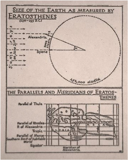
FIGURE 3.2 Eratosthenes’ technique for determining the size of Earth. SOURCE: The Eratosthenes Project, http://www.phys-astro.sonoma.edu/observatory/eratosthenes/#original.
with an origin at the center of Earth and measured the relative orientation of sunlight as it struck Earth. The key to his spatial analysis was the measurement of angles relative to a plane perpendicular to a radius to the center of Earth, an absolute measure of direction (Figure 3.2).
The debates over his data (e.g., the interpretation of the distance of a stade and the accuracy of the distance measurement) and the fact that Alexandria and Syene do not lie on the same meridian are incidental to the magnitude of his achievement. It is the integration of geography and geometry, the use of observation and empirical data, the use of a superb sense of spatial intuition, and the marriage of deduction and calculation that make Eratosthenes’ feat quite remarkable. From a few pieces of data and some beliefs, he used the power of spatial thinking to capture the size of Earth.
3.5.4 The Next Steps: The Spatial Structure of the Solar System
From this work on the shape and size of Earth, the next 2,000 years were marked by a struggle to come to grips with the spatial structure of the solar system. The search was an interesting one from the perspective of spatial thinking. Frequently, this search for an understanding of the structure of the solar system is described as a process of replacing the geocentric view of the universe with a heliocentric view. In a more fundamental spatial view, the search illustrates the power and implications of selecting an appropriate frame of reference.
From the time that individuals began to make systematic observations of the objects in the sky, and until the time of Copernicus, the crucial task of astronomers was predicting the position of the moving celestial bodies as a function of time. These predictions were essential for their primary functions of time keeping, eclipse prediction, and generating horoscopes. The Ptolemaic universe, the dominant geocentric cosmology for many centuries, is a spatialization of a method used to predict the position of various celestial objects, such as the Moon and the planets that appeared to move against the backdrop of the fixed stars. In general, the “fixed stars” tended to retain their positions with respect to one another on an imaginary “celestial sphere,” which appeared to turn slowly around Earth, making one circuit every 24 hours. In contrast, the planets (then taken to be the Sun, Moon, Mercury, Venus, Mars, Jupiter, and Saturn) appeared to move irregularly with respect to the stars. The Sun and Moon always moved in one direction with respect to the stars, while the other planets moved at different speeds and sometimes even moved backwards (retrograde motion). Furthermore, the planets Mercury and Venus were never seen far from the Sun. These features were well known even to the earliest observers, and any explanation of the structure of the solar system had to explain these motions.
The Ptolemaic system, set forth by Claudius Ptolemy in the Almagest around AD 150, was a refinement of earlier ideas. The major feature of the Ptolemaic system was the use of epicycles (Figure 3.3), or circles on circles, as a mathematical device to predict where a planet would be at any given time. The appropriate choice of epicycles could explain why Mercury and Venus were never seen too far from the Sun and could even explain the retrograde motion of the planets. The result was a remarkably good description of the relative motion of the objects in the solar system from the frame of reference of Earth.
The major feature of the Ptolemaic view was the use of epicycles (Figure 3.4) to explain the retrograde motion of the outer planets (Figure 3.5). In essence, however, the result is simply a description of the relative motion of the objects in the solar system from the frame of reference of Earth.
The Copernican cosmology can be viewed as a simple transformation of the motion of the same objects to the frame of reference of a fixed Sun. To the extent that the models of these respective universes are calibrated by observations, they have the same predictive power for a terrestrial observer interested in prediction. However, several steps, theology aside, led to the acceptance of the Copernican model. First, its elegant spatial simplicity was appealing. Next, the laws of planetary motion, derived from the model by Kepler, gave it some deeper appeal. Kepler’s laws were significant spatial generalizations about the relationships between the planets and the Sun. He not only inferred the elliptical nature of the orbits of the planets, but also provided a generalization that explained the orbits of all objects in terms of the period of rotation around the Sun and their distance from the Sun. By adopting elliptical orbits in a heliocentric system, Kepler was the first to be able to explain the retrograde orbit of the outer planets in modern terms (Figure 3.5). Finally, through the application of the theory of gravitation, Newton gave the Copernican system grounding in first principles, assigning primacy to the mass of the Sun as a referent for the entire solar system.
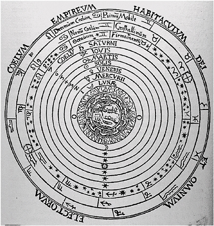
FIGURE 3.3 Ptolemaic system. The basic ordering of the planets around Earth is a feature of the Ptolemaic system. SOURCE: http://abyss.uoregon.edu/~js/glossary/ptolemy.html. Reproduced by permission of the Whipple Library, University of Cambridge.
3.5.5 Next Steps: Distances Beyond the Solar System
The next step in building a picture of the universe depended on creating a distance scale that could accommodate distances beyond the solar system. The key method for doing so involved the concept of astronomical parallax (Figure 3.6). From the perspective of spatial thinking, the measurement of astronomical parallax plays an interesting role in resolving the debate between the geocentric and heliocentric models of the solar system.
The essential challenge of astronomical observation in the middle of the second millennium was the accurate measurement of the position of the planets and the stars. The master of this challenge was Tycho Brahe. At his observatory, Uraniborg, he assembled the most accurate instruments of the day for his observations, observations that made Kepler’s work possible. Tycho, who arguably had the best understanding of the relative positions of the astronomical objects of the time, opposed the Copernican view because he was unable to observe stellar parallax. His observations of stellar positions were by far the most accurate of the time and, therefore, he would have been the
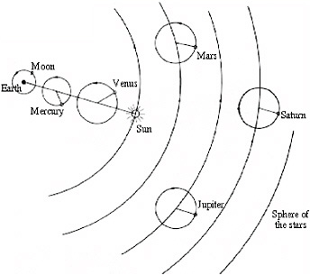
FIGURE 3.4 Epicycles in the Ptolemaic system. SOURCE: http://abyss.uoregon.edu/~js/glossary/ptolemy.html. Reproduced by permission from Dr. Jose Wudka.
FIGURE 3.5 Retrograde motion. In modern heliocentric theory, the relative motions of the planets around the Sun causes the outer planets, those further away from the Sun than Earth, to appear to move backwards relative to the fixed stars on a regular basis. Note also that the inner planets are never seen at a large angular separation from the Sun. These two features were well known even to prehistoric observers, and any explanation of the structure of the solar system had to explain these motions. SOURCE: Abell, 1969.
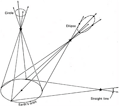
FIGURE 3.6 Astronomical parallax. The measurement of astronomical parallax is a triangulation of the distance to a star, using the orbit of Earth around the Sun as a baseline. A star is said be 1 parsec away if the angle p is 1 second of arc. Tycho’s difficulty with measuring this angle was that it was well below the limit of his ability to detect. The nearest star is Proxima Centauri, 1.3 parsecs away, making the parallax angle less than 1 second. In practice this technique works only for relatively nearby stars, and the parallactic motion is measured against stars much further away that have no detectable parallax. SOURCE: Abell, 1969.
most likely to detect stellar parallaxes. However, the largest observed stellar parallax is less than 1 second of arc and 60 times smaller than the limit of Tycho’s instrumentation of approximately 1 arc minute. The detection of stellar parallax led to the eventual proof that not only was Earth not the center of the universe, but the Sun was just an ordinary star of modest luminosity.
The breakthrough came in 1838 when three astronomers—Bessel, Henderson, and Struve—reported measuring the parallax of three nearby stars, 61 Cygni, Alpha Centuri, and Vega. This measurement served two critical purposes. First, it established the parsec as the basic unit of astronomy. Using the Sun-Earth distance as the baseline, a parsec is defined as the distance at which an object would have a parallax of 1 arc second, a distance equal to 206,265 times the distance of Earth from the Sun. Second, it established the scale of the universe, as then perceived, to be very large. The nearest stars were found to be more than 1 parsec away.
Following the first detection of stellar parallax, astronomers slowly began to build up a picture of the solar neighborhood, the region around the Sun where the parallax of objects could be measured. Edward Hertzsprung in 1911 and, independently, Henry Norris Russell in 1913 gave astronomy its first astrophysical spatialization—the Hertzsprung-Russell (H-R) diagram (Figure 3.7). This diagram plotted absolute magnitude against the newly identified spectral type of nearby stars. Two key concepts were merged in the diagram. The first was that of absolute magnitude,
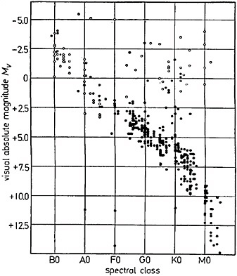
FIGURE 3.7 The Hertzsprung-Russell (H-R) diagram. Developed independently by the two astronomers for whom it is named, the H-R diagram shows absolute magnitude versus spectral type. Since the spectral type is a surrogate for temperature, hot blue stars are found on the left of the diagram and cool red stars on the right. The Sun is a star of intermediate temperature (G spectral type) with an absolute magnitude of approximately 5. The group of stars running from upper left to lower right is called the main sequence and is where most stars are found on the diagram. A simple consideration of the Stefan Boltzman law suggests that a star above the main sequence at the same spectral type (temperature) must be large and one lower is smaller. This led to the designation of the stars in the upper right as red giants and those in the lower left as white dwarfs. Later work showed that the position in the H-R diagram was a product of stellar mass and age. The magnitude scale is a logarithmic scale of luminosity. Stars whose absolute magnitude differs by 5 differ in intrinsic luminosity by a factor of 100. SOURCE: Unsöld, 1969.
which is simply the brightness of a star if it were placed at a standard distance of 10 parsecs. Examining the visible spectrum of a star and classifying it according to the observed distribution of features seen in its spectrum determines the spectral type of the star. Second, as ideas of modern quantum mechanics explained the reason for the existence of different spectral features in stellar spectra, it was realized that the star’s spectral type was a surrogate for temperature, so that the horizontal axis of the H-R diagram ran from hot blue stars on the left to cool red stars on the right. When spectral type and absolute magnitude were plotted, most stars were found to fall on a single broad band, called the main sequence, with some hot dim stars found below the main sequence and some cool bright stars found above. In one diagram, therefore, the concept of red giant and white dwarf stars was given meaning.
Over the next several years, there were two approaches to building a picture of the structure of the universe, as revealed by the distribution of the stars. Both approaches involved the concept of a “standard candle,” thus establishing the absolute brightness (magnitude) of a star by nonparallax means. Using the absolute and the apparent brightness, it was possible to infer the distance of the star. Both methods were tied to stars whose parallax had been measured, but they allowed the extension of the distance scale beyond the solar neighborhood and the reach of the measurement of parallax.
One approach built on the H-R diagram and developed what became known as “spectroscopic parallaxes.” In this approach, the spectrum of a star was examined and then classified. By the time of the development of this method, it had been shown that spectra gave evidence not only of the temperature but also of the luminosity of a star. For example, it was possible from an examination of a star’s spectrum to distinguish between a main sequence star of spectral K0 (Figure 3.7) and a brighter (giant) star of the same temperature. So, by observing a star’s spectrum, we know about how bright it is if seen from a given distance. By comparing its known absolute brightness with its apparent brightness in the sky, we can infer how far away it is. In fact, the classification approach was sufficiently precise that the magnitude of a star’s absolute brightness could be established within approximately 10–25 percent (a few tenths of a magnitude) and the distance inferred to comparable accuracy.
In 1953, Morgan, Whitford, and Code used this technique of spectroscopic parallax to map the spatial distribution of young clusters of stars around the Sun (Figure 3.8). This analysis shows the distribution of these objects forming three distinct arms, and it was a key step in creating a sense of the spatial structure of our galaxy.
The second set of standard candles emerged through yet another astrophysical spatialization, called the period-luminosity diagram (Figure 3.9). This approach was made possible by Leavitt’s observation in 1911 that the period of a particular class of pulsating stars is an excellent predictor of its average absolute magnitude. This class of stars, called Cepheids after the prototype delta Delta Cephei, is also easy to identify from its distinctive light curve (the change in brightness over the period of pulsation) (Figure 3.10). Leavitt made her discovery by observing Cepheid variables in a nearby galaxy, the Small Magellanic Cloud. Because the distance of these variable stars relative to each other was small in comparison to their absolute distance from Earth, the scatter in their distance did not hide the relationship.
In 1924, Edwin Hubble used this new standard candle and the 100-inch telescope on Mount Wilson to identify Cepheids in the Andromeda Nebula (Figure 3.11), establishing once and for all that it was a galaxy like our own.
Hubble went on to extend his system of standard candles and measures to establish the distances to increasingly distant galaxies. In 1929, Hubble made a discovery that opened up the universe even further and thus began the age of modern cosmology. He found that the further a galaxy was from Earth, the faster it was moving away (Figure 3.12).
This led to the idea of an expanding universe, which in turn led to the “Big Bang” theory—that the universe was once all together, in a single place. With the discovery from this picture of an expanding universe, astronomy moved on to concepts such as the Big Bang, the discovery of quasars and other objects moving at very high velocities relative to Earth. The Hubble relationship became not only a map of space, but also a map of time. More distant objects, because of the finite velocity of light, are being observed at an earlier time in the history of the universe, opening up a window into the evolution of galaxies and clusters of galaxies and the “three degree” background radiation.
However, it is interesting to note that the “Hubble Constant,” the quantity that describes the expansion velocity of the universe, has the units of kilometers per second per megaparsec (a million
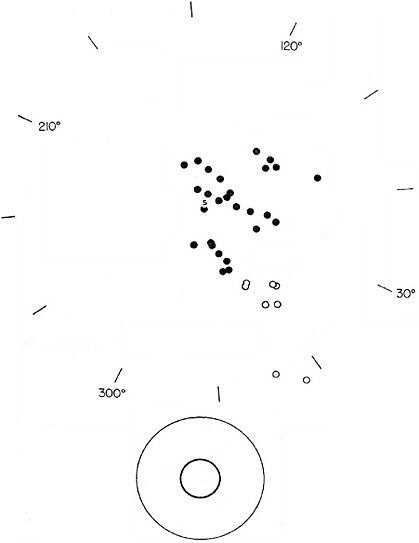
FIGURE 3.8 Map of the solar neighborhood. This diagram projects the position of younger clusters of stars onto the galactic plane. The Sun is denoted by S in the diagram. From observations of external galaxies we know that the spiral arms are apparent largely because of the presence of bright stars in relatively young clusters of stars. In showing the position of these stars near the Sun we can see a similar pattern. Parts of three arms of our galaxy are visible from the diagram. SOURCE: Morgan et al., 1953, p. 318. Reproduced by permission from the American Astronomical Society.
parsecs). So even in our description of the far reaches of the universe, the distance scale is tied to the distance from Earth to the Sun. This distance scale is an appropriate homage to the process of spatial thinking that led from measuring the diameter of Earth to an understanding of some of the most fundamental properties of the universe.

FIGURE 3.9 The period-luminosity diagram for the Cepheids. This diagram shows Henrietta Leavitt’s graph of data for the Small Magellanic Cloud. It illustrates the relationship between the period of a Cepheid variable and its average luminosity. Left: m refers to the average apparent magnitude of the variable as observed; right: M refers to absolute magnitude of the variable stars. SOURCE: http://www.astro.livjm.ac.uk/courses/one/NOTES/Garry%20Pilkington/cepinp1.htm.
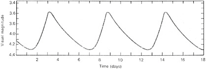
FIGURE 3.10 The characteristic light curve of a Cepheid variable. This star has a period of approximately 5.5 days (log 0.74), which implies that it has an absolute magnitude of approximately −1.5. Recalling from Figure 3.9 that the magnitude scale is a logarithmic scale of luminosity and that stars whose absolute magnitude differs by 5 differ in intrinsic luminosity by a factor of 100, we can calculate the distance to the star. The average apparent magnitude (visual magnitude in the figure) is 3.75, making the difference between absolute and apparent magnitude slightly more than 5. Therefore, the star appears approximately 100 times less luminous than it would if it were at the standard distance of 10 parsecs. Applying the inverse square law (luminosity decreases in proportion to 1/r2), one can infer that this star would be slightly more than 100 parsecs away. SOURCE: Abell, 1969, p. 480.
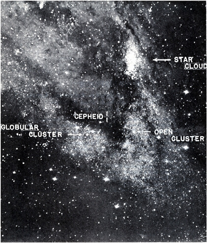
FIGURE 3.11 Cepheids in the Andromeda galaxy. Using the 100-inch Hooker telescope at Mt. Wilson, Hubble managed to measure the light curves of variable stars in the Andromeda galaxy, which he identified as Cepheids, and used to infer the distance to the galaxy. SOURCE: Hubble, 1936.
3.5.6 Thinking Spatially in Astronomy: The Role of Astrophysical Spatialization
Astronomy has at its core a long and powerful practice of spatial thinking. Two factors enabled its advancement: (1) a careful and systematic observation of the heavens and (2) a series of intellectual breakthroughs achieved by some of the finest spatial thinkers in the history of science. Breakthroughs enabled astronomy to build a picture of the universe in space and time, starting from the seemingly simple observation of the apparent position and brightness of celestial objects in the night sky. The boundary of our knowledge of the four-dimensional structure of the universe spread out from Earth like a ripple from a rock thrown in the pond. Eratosthenes’ work provided a baseline, the shape and size of Earth. Kepler used the observations of Brahe to build a rational view of the spatial structure of the solar system and the motion of planets and other objects within it. With time,
FIGURE 3.12 The redshift distance relationship. This diagram shows that galaxies further away are receding from our galaxy at faster rate. The slope of the relationship is given by the Hubble constant (H) measured in kilometers per second per megaparsec. The inverse of the Hubble constant is a simple estimate of the age of the universe. SOURCE: Hubble, 1936.
these efforts created distance scales to accommodate distances beyond the solar system: moving from the solar neighborhood to another spatial context, that of our galaxy, and finally, to a vision of an expanding universe enabled by Edwin Hubble’s work. At this scale, distance becomes time. Thus, spatial thinking brought us not only a picture of the spatial structure of the Universe, but an understanding of its history as well.
3.6 SPATIAL THINKING IN GEOSCIENCE
3.6.1 Thinking Spatially in Geoscience: The Operations
As with any complex scientific practice, it is difficult to identify the component operations and impossible to specify a single sequence in which they are performed. Based on the experience of geoscientists, the committee presents a descriptive catalog of the spatial thinking operations typically performed in the process of doing geoscience. It is based on two categories of thinkers: expert geoscientists, especially those undertaking a spatial challenge that is novel to anyone, and beginning students, undertaking a spatial challenge that is novel to them. Thinking spatially by geoscientists and geoscience students involves, among other things,
-
describing the shape of an object, rigorously and unambiguously;
-
identifying or classifying an object by its shape;
-
ascribing meaning to the shape of a natural object;
-
recognizing a shape or pattern amid a cluttered or noisy background;
-
visualizing a three-dimensional object or structure or process by examining observations collected in one or two dimensions;
-
describing the position and orientation of objects you encounter in the real world relative to a conceptual coordinate system anchored to Earth;
-
remembering the location and appearance of previously seen items;
-
envisioning the motion of objects or materials through space in three dimensions;
-
envisioning the processes by which objects change shape;
-
using spatial thinking to think about time; and
-
considering two-, three-, and four-dimensional systems where the axes are not distance.
Describing the Shape of an Object, Rigorously and Unambiguously
Untold person-lifetimes have been invested in the task of describing natural objects in a way that is rigorous and unambiguous, and attends to all of the important observable parameters. Faced with the huge range of objects found in nature, mineralogists, petrologists, geomorphologists, structural geologists, sedimentologists, zoologists, and botantists had to begin by agreeing upon words, measurements, and concepts with which to describe these natural objects.
Given a collection of objects that intuitively seem related in some way, what should you observe, and what should you measure, in order to capture the shape of each object? After much spatial thinking, crystallographers decided that you should observe how many planes of symmetry the crystal has and whether or not the angles between those planes of symmetry are right angles. Size and color of the crystal are not so important (Figure 3.13). After much spatial thinking, structural geologists decided that you should describe a fold in a sedimentary layer by imagining a plane cutting through the axis of symmetry of the fold, and then measuring the dip and strike of this plane, and the plunge of the intersection between this axial plane and the fold itself (Figure 3.14).
Although this descriptive style of geoscience and biology tends to be disparaged nowadays, the worldwide effort, in the eighteenth through twentieth centuries, to develop methodologies describing the objects of nature was crucial to the success of the discipline.
The processes on the part of expert observers as they develop a new description methodology include (1) careful observation of the shape of a large number of objects; (2) integrating these observations into a mental model of what constitutes the common characteristics among this group of objects; (3) identifying ways in which individual objects can differ while still remaining within the group; and (4) developing a methodical, reproducible set of observation parameters that can describe the range of natural variability within the group, thus defining a class. Step (4) may include developing a lexicon or taxonomy of terms, developing measuring instruments, developing units of
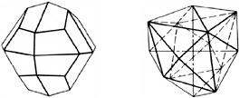
FIGURE 3.13 Describing the shapes of natural objects, rigorously and unambiguously: stereograms of crystals. SOURCE: Hurlbut, 1971. Copyright © 1971 by C. S. Hurlbut. Reproduced by permission of John Wiley & Sons, Inc.
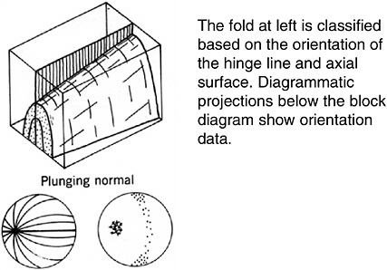
FIGURE 3.14 Describing the shapes of natural objects, rigorously and unambiguously: classification of folds. SOURCE: Hobbs et al., 1976.
measurement, and/or developing two-dimensional graphical representations of some aspect of the three-dimensional objects.
For the novice, developing this descriptive skill involves becoming facile with the terms and techniques used by specialists who have previously studied this class of objects. In some cases, these descriptive techniques call upon projective and Euclidean spatial skills that many learners find extremely difficult. For example, when structural geologists collect data on which to apply their fold classification system, they record the vector that is perpendicular to the surface of the fold at many points on the fold, mentally extend those vectors until they intersect an imaginary hemisphere beneath the fold, and convey this information as points on a lower-hemisphere equal-area projection diagram. Command of projective spatial skills is required either to record or to interpret such data (Figure 3.15).
Similarly, many students have difficulties in spotting the subtle planes of symmetry that are required to make use of the crystallographers’ descriptive methodology. Then, when it comes time to describe the angular relationships between crystal faces (using a system called Miller indices in which the three faces of a cube, for example, are labeled 001, 010, and 100) most students find that their Euclidean spatial ability initially fails them (Figure 3.13).
Identifying or Classifying an Object by Its Shape
Paleontologists or micropaleontologists identify fossils or microfossils according to shape or morphology. A variant of this task is identifying an object according to its shape, texture, and color. Mineralogists or petrologists identify minerals in a hand sample or photomicrograph by their shape, their color (including how their color changes under different lighting conditions), and their texture
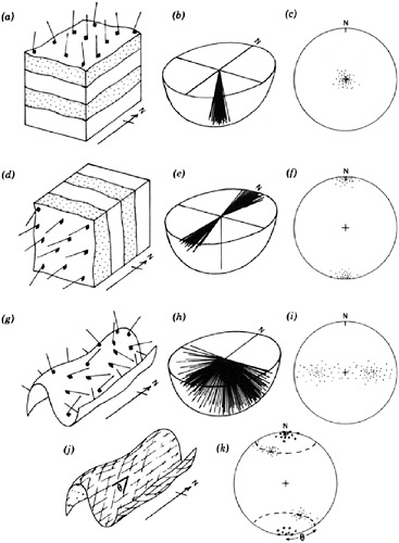
FIGURE 3.15 Diagrammatic representation of equal-area projection of various fabric elements. SOURCE: Hobbs et al., 1976.
(e.g., Does it have stripes? Does it have a shiny surface?). However, individual grains of the same mineralogy and individual fossils of the same species are not identical, but tend to share certain diagnostic properties (e.g., plagioclase grains tend to be much longer than they are wide, whereas olivine grains tend to be roughly as long as they are wide) (Figure 3.16).
Novices learn this identification skill by comparing unknown fossils or minerals against a physical catalog, using the descriptive terms and measurements mentioned above. To become experts, students must construct a mental catalog of the properties of dozens to hundreds of fossils or minerals, and then develop facility at comparing each unknown new mineral or fossil against this mental catalog.
FIGURE 3.16 Flow chart for identifying minerals. SOURCE: Marshak, 2002. Earth Portrait of a Planet, New York, W.W. Norton & Co. Inc., Appendix B-2 Flow Charts for Identifying Minerals.
Ascribing Meaning to the Shape of a Natural Object
The shape of a natural object found in situ (including its size and orientation) carries clues about its history and formative processes.
One of the most famous instances of ascribing meaning to the shape of a natural object is the work of Alfred Wegener (1880–1930). He noted the apparent jigsaw-like fit of the coastlines of Africa and South America, and inferred that the continents were previously connected (Wegener, 1929) (Figure 3.17). James Hutton (1726–1797) noted the contrast in shape and texture of underlying and overlying rocks at his famous Scottish outcrop, and inferred the existence of unconformities and thus the immensity of geologic time (Hutton, 1788) (Figure 3.18). Both instances reflect brilliant spatial thinking.
In everyday practice, micropaleontologists use morphologic clues to make inferences about the geologic age and the paleoenvironment within which planktonic microfossils lived and died (Figure 3.19). One group of diatom (a form of phytoplankton) fossils might have thick silicate shells, whereas another group of diatoms has delicate thin shells. This difference could be attributed to the latter group’s growing in water impoverished in dissolved silicon or it could be an evolutionary difference. The carbonate-shelled microfossils (foraminifera) in a sediment sample might be pitted and lack delicate protruberances (Figure 3.20). This could be attributed to the sediment sample being deposited near the calcite compensation depth, the depth in the ocean below which calcium carbonate dissolves and above which calcium carbonate is preserved in sediment. The observation that a group of microfossils are much smaller than typical for their species could be attributed to their living in a stressed environment, for example a marine species living in brackish water.
Structural geologists look at distortions in the shapes of crystals and fossils to infer the strain (and thereby stress) that a body of rock has undergone (Figure 3.21). Sedimentologists use the presence of ripples and other sedimentary structures to infer that a sedimentary stratum was depos-
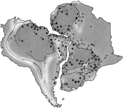
FIGURE 3.17 Ascribing meaning to the shape of a natural object: jigsaw-like fit of the coastlines of Africa and South America. SOURCE: Hamblin, 1994. Reprinted by permission of Pearson Education, Inc., Upper Saddle River, N.J.
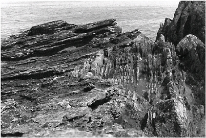
FIGURE 3.18 Ascribing meaning to the shape of a natural object: Siccar Point. SOURCE: Dr. Clifford E. Ford, 2004, http://www.geos.ed.ac.uk/undergraduate/field/siccarpoint/images.htm.
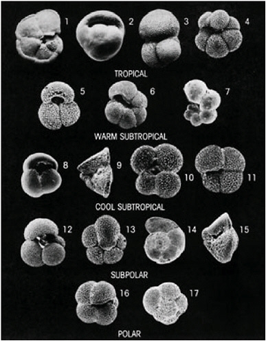
FIGURE 3.19 Ascribing meaning to the shape of a natural object: distribution of modern species of planktonic foraminifera. SOURCE: Kennett, 1982. Reprinted by permission of Pearson Education, Inc., Upper Saddle River, N.J.
ited under flowing water, and they use the orientation and asymmetry of the ripples to determine which way the current was flowing in the ancient body of water. Whether a river is meandering, straight, or braided tells geomorphologists about the energy regime (velocity) of a river. Similarly, the grain-size distribution of sedimentary particles tells sedimentologists about the velocity of an ancient river; it takes a higher energy flow to carry gravel rather than sand.
To summarize from these examples, the shape of a natural object can be influenced by (1) its strain history, (2) the energy regime under which it was formed, (3) the chemical environment under which it formed, and (4) changes in the physical or chemical environments experienced after its initial formation. Geoscientists seek to reason backwards from observing the morphology to
FIGURE 3.20 Ascribing meaning to the shape of a natural object: carbonate-shelled microfossils. SOURCE: Kennett, 1982. Reprinted by permission of Pearson Education, Inc., Upper Saddle River, N.J.
inferring the influencing processes. The key questions are: What processes or forces could have acted upon this mineral, landform, fossil, or organism (the fossil before it died) to cause it to have this shape? What function could this form have served in the life of the organism?
The novice generally begins by applying learned rules of thumb. At the expert level, this thought process involves reasoning from first principles about the connection among form, function, and history and doing so in the context of an expert knowledge base about the normal characteristics of the class of objects under study. Students, as novices however, may misunderstand fundamental processes (Figure 3.22). The ability to reason from first principles well is one of the abilities people have in mind when they say that someone has good “geologic intuition.”
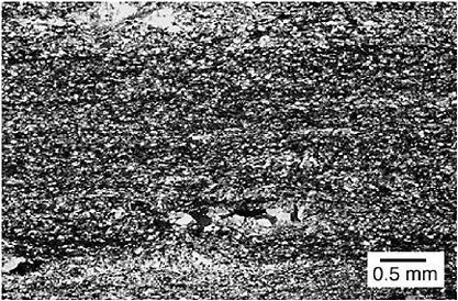
FIGURE 3.21 Ascribing meaning to the shape of a natural object: the shape and orientation of the mineral grain in this photomicrograph are interpreted as evidence that the rock has undergone shearing. SOURCE: The University of North Carolina, Chapel Hill, Department of Geological Sciences.
Recognizing a Shape or Pattern amid a Cluttered or Noisy Background
An experienced interpreter of seismic reflection data can confidently and reproducibly trace seismic reflectors across a graphic profile that looks like uniform gray noise to the untrained eye (Figure 3.23). A gifted paleontologist can stand at an outcrop with a bus full of geologists and spot fossils where others see nothing.
Visualizing a Three-Dimensional Object, Structure, or Process by Examining Observations Collected in One or Two Dimensions
Physical oceanographers measure the temperature and salinity of seawater by lowering an instrument package on a wire vertically down from a ship and recording the temperature, conductivity, and pressure at the instrument. Thousands of vertical conductivity-temperature-depth profiles have been combined to create our current understanding of the three-dimensional interfingering of the water masses of the world’s oceans.
A field geologist examines rock layers and structures where they are exposed at Earth’s surface in outcrop, taking advantage of differently oriented road cuts, stream cuts, wave cuts, or quarries to glimpse the third dimension. From these fragmented surficial views, he or she constructs a mental view of the interior of the rock body or, more commonly, multiple possible views.
The expert’s visualization of the parts of a structure that cannot be seen is guided by more than simple mechanical interpolation between observable sections or profiles. The physical oceanographer’s visualization is, for example, shaped by physics that decrees that lower-density water masses overlie higher-density water masses (Figure 3.24). The field geologist’s visualization is shaped by the understanding that marine sedimentation processes tend to produce layers roughly horizontal and roughly uniform in thickness before deformation. Marie Tharp’s case (see Section 3.7)
FIGURE 3.22 Ascribing meaning to the shape of a natural object: reasoning from first principles. SOURCE: Kusnick, 2002.
is interesting because neither she nor anyone else knew any details about the tectonic and volcanic processes that form the seafloor geomorphology; yet her maps in areas of sparse data (the Southern Oceans, for example) are far better than would have been possible by interpolating from data alone. In these examples, the physical oceanographer and the field geologist are guided by knowledge of the processes that shaped the unseen parts of the puzzle, but in Tharp’s case she seems to have developed a spatial intuition or feel for the nature of the seafloor before the formative processes were understood.
Describing the Position and Orientation of Objects Encountered in the Real World Relative to a Conceptual Coordinate System Anchored to Earth
Learning to measure the dip and strike of a sedimentary strata or other planar surface is a rite of passage for introductory geoscience students (Figure 3.25). This technique requires Euclidean spatial skills (see Appendix C). Many students seem incapable of grasping this technique at any kind of deep or intuitive level; at best, they can learn to memorize a sequence of steps and apply them mechanically.
Until the advent of GPS navigation for research vessels, navigation was a huge issue for seagoing oceanographers. The challenge is to make the most precise seafloor maps, ground-truthed
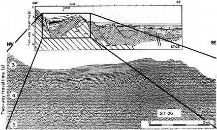
FIGURE 3.23 Recognizing a shape or pattern amid a cluttered, noisy background. Multichannel seismic line ST06 across a small tilted block at the base of the Monte Baronie structure. SOURCE: Rehault et al., 1987.
FIGURE 3.24 Visualizing a three-dimensional object, structure, or process by examining observations collected in one or two dimensions.
with the most precisely located samples, measurements, and photographs. This requires navigational understanding of ships, samples, and towed vehicles. Every navigation technique—dead reckoning, sextant, Loran, doppler satellite navigation, seafloor-based acoustic transponders, or GPS—requires thinking about how angles and/or distances change as a function of the relative motions between objects.
This suite of tasks is difficult because it involves angular estimations. Dealing with angles is a skill that can be improved with practice and lost through disuse. As a result of practice, a marine geologist can learn to estimate a compass course on a map by eye to within better than 5 degrees,
FIGURE 3.25 Describing the position and orientation of objects in the real world relative to a coordinate system anchored to Earth.
changes of heading to within 1 degree, and then mentally integrate the angular effect of wind, current, and wire pull on the ship’s heading.
Learning how to figure out where you are on a topographic map is another rite of passage for geology students. This skill has a real life counterpart in figuring out where you are on a road map. The mental process involves making connections between the three-dimensional, horizontally viewed, infinitely detailed, ever-changing landscape that surrounds you and through which you are moving, and the two-dimensional, vertically viewed, schematic, unchanging representation of that landscape on a little piece of paper. Although navigating through an unfamiliar terrain by referring to a map is probably the most common map-using task for nonprofessional map users, this skill is rarely taught in school.
Remembering the Location and Appearance of Previously Seen Items
The great Appalachian field geologist John Rodgers (Rodgers, 2001) knew the location of every outcrop and every ice cream stand from Maine to Georgia. Students recall that he remembered the salient sedimentary and structural characteristics of every outcrop he had ever seen in any mountain range in the world, and where it was located. His ability to remember the relationships among rock bodies at those outcrops allowed him to construct, over a long lifetime in the field, a mental catalog of occurrences of geologic structures, which he drew on to create a masterful synthesis of how fold-and-faulted mountain ranges form (Rodgers, 1990).
William Smith (1769–1839) made the world’s first geological map (Figure 3.26), a map of England and Wales showing rocks of different ages in different colors (Winchester, 2001). When Smith began his field work, it was not understood that rocks occurred on Earth’s surface in organized spatial patterns; he figured out that the organizing principle was the age of the rocks as recorded in their fossils. As with Marie Tharp, Smith made his map before the causal processes that underlay the observations on his map were understood, and he worked from incomplete data, primarily outcrops revealed in canal cuts. As with Marie Tharp’s map, Smith’s map stands up very well to comparison with modern maps. Many spatial skills must have contributed to Smith’s effort,
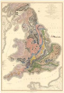
FIGURE 3.26 William Smith’s geological map of England and Wales. SOURCE: Winchester, 2001.
but among them was his ability to remember and organize, aided only by the simplest of paper and pencil records, a huge body of spatially referenced observations. His nephew, John Phillips, wrote of William Smith: “A fine specimen of this ammonite was here laid by a particular tree on the road’s side, as it was large and inconvenient for the pocket, according to the custom often observed by Mr. Smith, whose memory for localities was so exact that he has often, after many years, gone direct to some hoard of nature to recover his fossils.” [emphasis added] (from Memoirs of William Smith by John Phillips cited in Winchester, 2001, p. 270).
Envisioning the Motion of Objects or Materials Through Space in Three Dimensions
Physical oceanographers and marine geochemists envision water moving along the “great ocean conveyor belt” of density-driven ocean currents (Broecker, 1991). Atmospheric physicists envision a spiraling pattern of air currents in latitudinally bounded bands. Geophysicists envision mantle rising beneath ridge crests and sinking at subduction zones. Today’s students have brightly colored textbook drawings and animated web sites to help them visualize these complex three-dimensional flows. The first thinkers to envision these flows, which cannot be seen literally even in part by human eyes, must have made gigantic leaps of spatial thinking.
For these pioneer thinkers, to what extent did the visualization grow from data and to what extent from understanding of causative processes? The simplistic notion is that one collects a mass of data about the distribution of some property or process, combines the data into a mental picture or computer-aided visualization, and then interprets it. This may understate and underestimate the skill of a spatial thinker.
Consider the example of global atmospheric circulation. Certainly, the existence and orientation of trade winds, a fundamental observation, was known from long ago. Yet the northward counterflow at high altitude cannot have been documented observationally by those pioneers; they must have inferred it and included it in their mental picture because the picture did not make physical sense without it. Some of the great leaps of visualization of three-dimensional Earth processes have progressed by a hybrid process, in which the visualization is partly shaped by data and observations and partly by intuitive understanding of driving forces. Modern models of oceanic and atmospheric circulation try to formalize this hybrid cognitive process. The models are built around equations that purport to represent physical forces, and then data are used to “train” the models through a process of “data assimilation.”
Envisioning the Processes by Which Objects Change Shape
Whereas the fluid parts of the Earth system generally respond to imposed forces by moving through space, the solid parts may respond by changing their shape, by deforming, by folding, and by faulting. After struggling to visualize the internal three-dimensional structure of a rock body, the geologist’s next step is often to try to figure out the sequence of folding and faulting events that has created the observed structures. This task may be attacked either forwards or backwards: backwards, by “unfolding” the folds and “unfaulting” the faults; or forwards, by applying various combinations of folds and faults to an initially undeformed sequence of rock layers until you find a combination that resembles the observed structure (Figure 3.27). The forward approach resembles the paper-folding task used by psychologists who study spatial thinking (see Chapter 2).
Elements of solid Earth also change their shape through erosion, through the uneven removal of parts of a whole. Thinking about eroded terrains requires the ability to envision negative spaces, the shape and internal structure of the material that is no longer present.
Using Spatial Thinking to Think About Time
It is common in thinking about Earth to find that variation or progression through space is closely connected with variation or progression through time. For example, within a basin of undeformed sedimentary rocks, the downward direction corresponds to increasing time since deposition. On the seafloor, distance away from the mid-ocean ridge spreading center corresponds to increasing time since the formation of that sliver of seafloor.
As a consequence, geologists often think about distance in space when they really want to think
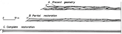
FIGURE 3.27 Mentally manipulating a volume by folding, faulting, and eroding: geometry of the lower duplex at Hénaux. SOURCE: Ramsay and Huber, 1987. Copyright 1987, reprinted with permission from Elsevier.
about duration of geological time. Distance in space is easy to measure, in vertical meters of stratal thickness or horizontal kilometers of distance from ridge crest. Duration in geological time is hard to measure, and subject to ongoing revision, involving complicated forays into seafloor magnetic anomalies, radiometric dating, stable isotope ratios, or biostratigraphy.
In another kind of interaction between space and time, geologists use spatial relationships in rock bodies to figure out the sequence of events. If a volcanic dike cuts across certain layers of sedimentary rocks, then the intrusion of the dike must have happened after the deposition of the sediments. Sediments in a fault-bounded basin that form a wedge, in which the deeper layers dip more steeply than the shallow layers, are interpreted as “syn-rift” sediments, sediments deposited during the interval of time when the basin’s bounding normal faults were slipping.
Considering Two-, Three-, and Four-Dimensional Systems Where the Axes Are Not Distance
Specialists within different branches of geosciences have a tendency to use “space” as a metaphor for variation in observable but nonspatial parameters of natural systems. For example, petrologists visualize a tetrahedron, in which each corner is occupied by a chemical element or by a mineral of pure composition (e.g., one end member of a solid solution). Any given rock can be placed at a point within the tetrahedron according to the concentration of each of the components in the rock. To communicate this tetrahedron to colleagues, they project the data down onto one of the sides of the tetrahedron, where it appears on the page as a triangle, with each rock sample appearing as a dot.
Igneous petrologists deal in “pressure-temperature space.” The pressure dimension of this space is something like distance beneath Earth’s surface, but it is denominated in units of downwardly increasing pressure rather than in units of distance. The temperature dimension is also related to distance beneath Earth’s surface, with temperature increasing downwards. The chemical composition of an igneous rock depends in part on where in pressure-temperature space the initial melt separated out of the mantle.
Physical oceanographers deal in “T-S” diagrams, where T is the temperature and S the salinity of water mass. Temperature and salinity together control the density of the water mass, and density in turn controls whether the water mass will sink relative to other water masses in the same ocean. Water samples that share a common history will likely cluster together in T-S space, and water masses with different histories of formation will usually occupy different areas of T-S space.
The processes for thinking about these non-distance-denominated “geospaces” feel similar to the processes for thinking about the distribution of objects and their movement through “regular” distance space. A clue is that the vocabulary is the same. Two water masses are “close together” or “far apart” in T-S space. A body of rock in the mantle “moves” through pressure-temperature space on a “trajectory.”
This habit of mind of using spatial representations for nonspatial observables seems particularly common among geoscientists. People trained in other disciplines tend to use statistics, equations, or verbal descriptions to describe variability in the objects or systems they study, rather than the visually displayed, spatially based approaches so common in the geosciences.
3.6.2 Thinking Spatially in Geoscience: The Processes
Given this depiction of some of the operations of spatial thinking in geoscience, we can characterize spatial thinking as consisting of five major processes. These linked operations begin with observing, describing, recording, classifying, recognizing, remembering, and communicating the two- or three-dimensional shape, internal structure, orientation, and/or position of objects,
properties, or processes. The next step involves mentally manipulating those shapes, structures, orientations or positions—for example, by rotation, translation, deformation, or partial removal. The third step involves making interpretations about what caused the objects, properties, or processes to have those particular shapes, structures, orientations, and/or positions. With this understanding in mind, it is possible to make predictions about the consequences or implications of the observed shapes, internal structures, orientations, and/or positions. Finally, geoscientists can use spatial thinking processes as a short-cut, metaphor, or mental crutch to think about processes or properties that are distributed across some dimension other than physical space.
3.7 THINKING SPATIALLY IN GEOSCIENCE: THE SEAFLOOR MAPS OF MARIE THARP
3.7.1 Introduction: Seafloor Mapping
Marie Tharp (1920–) is a marine cartographer who made some of the first maps of the seafloor between the 1950s and the 1970s (Figure 3.28). With kilometers of water obscuring her direct vision, she was able to visualize and depict the shapes of terrain that no human eye had ever seen.
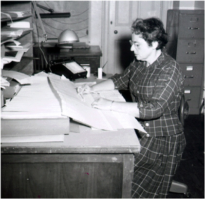
FIGURE 3.28 Marie Tharp in 1960. SOURCE: Columbia University, Earth Institute. World Ocean Floor, Bruce C. Heezen and Marie Tharp. Copyright by Marie Tharp 1977/2003. Reproduced by permission of the Marie Tharp Oceanographic Cartography, One Washington Ave., South Nyack, New York 10960.
Her maps have stood the test of time amazingly well when compared against modern maps made with sophisticated swath-mapping and satellite-based mapping systems.
She created the maps using sparse and flawed echograms based on echo sounder data and her remarkable capacity for spatial thinking. Tharp’s decades-long effort involved synthesizing vast amounts of spatial data, visualizing what was previously unseen, and interpreting spatial observations in terms of causal processes.
Marie Tharp worked at the Lamont-Doherty Earth Observatory of Columbia University in the research group of Professor Bruce Heezen. Earlier accounts (e.g., Menard, 1986) tended to give all or most of the intellectual credit to Heezen, recognizing Tharp only as the person who plotted the echograms. More recently, however, Tharp has been given credit for discovering the mid-Atlantic rift valley, correlating the rift valley and earthquake locations, and insisting on the validity of this as evidence for seafloor spreading at a time and place when this was considered to be heresy (Lamont-Doherty Earth Observatory, 2001).
3.7.2 The Nature of What Tharp and Heezen Did
Measure Water Depths from Precision Data Recorders (PDRs). Echo sounders measure the depth of the water beneath a ship by measuring the travel time of an electronic ping of sound as it travels from the ship to the seafloor and back. In Tharp’s era, the state of the art was the precision depth recorder, as refined by the U.S. Navy during World War II. The echoes from the seafloor were recorded as burn marks on a roll of paper by a stylus that swept across the paper once per second. Tharp and her assistants manually converted the location of these burn marks into water depths, measuring a water depth for each 5 minutes of time along the track of a ship’s travel.
Reconcile and Plot Navigation. Ship’s tracks were plotted by hand on table-sized plotting sheets at a scale of 4 inches to a degree of longitude, based on celestial navigation and dead reckoning by the ship’s officers. (On a modern research vessel, a navigation fix would be taken from the GPS every minute, the navigation would be logged by computer, and the ship’s track would be plotted automatically in real time.)
Plot Soundings on Navigation Plots. Water depths were written by hand onto plotting sheets, alongside the ship’s track.
Make Profiles and Contour Maps. Contours were drawn by hand on overlays of the plotting sheets. Profiles were made along azimuths that seemed interesting, sometimes combining segments of several different ship tracks to make a composite track (Figure 3.29). At this point we can begin to appreciate Tharp’s skill as a spatial thinker. Profiles and contour maps require judgments as to what is or is not interesting—which tracks to include or to discount.
Plot Complementary Data at the Same Scale. Earthquake epicenter location and sediment data were plotted, by hand, at the same scale as the bathymetric data. This strategy revealed that earthquakes and thin sediment cover occurred along the axis of the mid-Atlantic ridge.
Convert Profiles and Contours into Physiographic Diagrams. Heezen and Tharp’s most famous products are physiographic diagrams, scaled drawings or paintings of the seafloor as though all of the water had been drained away. Given the large gaps between track lines (tens to hundreds of kilometers even in the best covered areas; see Figure 3.30), creating a continuous physiographic diagram required substantial interpolation. Tharp gained a feel for the fabric or texture of the seafloor in areas of more abundant data and then used that “feel” to guide her mapping in the areas of less abundant data. We should note that this feeling was spatial or visual and intuitive, rather than being grounded in an understanding of the processes that formed the seafloor features because no-one understood those processes during the early years of Tharp’s mapping career.
The decision to use physiographic diagrams was initially motivated by the U.S. Navy’s classification and hence restriction of use of quantitative bathymetric data such as contours (Lawrence,
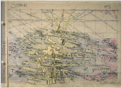
FIGURE 3.29 Tharp’s original hand contouring of a portion of the mid-Atlantic ridge. In the background, you can discern the tracklines with hand-written bathymetric sounding data points along them. Despite the sparseness of the tracklines, Tharp detected and depicted the rift valley along the axis of the mid-Atlantic ridge, which was one of the early lines of evidence for seafloor spreading. Tharp’s map also shows clearly the fabric of transform faults and fracture zones (the roughly east-west trends), although it was many years before an explanation of transform faults emerged. SOURCE: Library of Congress, http://www.loc.gov/exhibits/treasures/trr078.html.
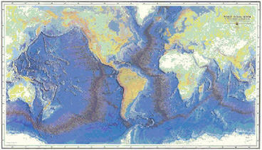
FIGURE 3.30 World ocean floor panorama. SOURCE: Heezen and Tharp, 1977. Copyright by Marie Tharp 1977/2003. Reproduced by permission of the Marie Tharp Oceanographic Cartography, One Washington Ave., South Nyack, New York 10960.
1999, 2002; Menard, 1986). In fact, however, the physiographic diagram approach proved to be a powerful visualization tool that probably facilitated the interpretation of morphology in terms of the formative processes. The physiographic diagrams foreshadowed the modern shaded-relief displays of digital elevation models.
Find Trends, Patterns, Consistencies, and Symmetries in the Data. The most famous example of this process was Tharp’s realization that the mid-Atlantic ridge has a deep, symmetrical, steep-sided valley running down its center. Heezen was at first unwilling to accept the existence of this valley, dismissing it as “girl talk” (Wertenbaker, 1974, p. 144), but after additional patient work, they were able to construct a compelling case for the widespread existence of this valley (Heezen and Tharp, 1956).
Interpret Physiographic Diagrams and Profiles in Terms of Formative Processes. The symmetrical, steep-sided valley in the mid-Atlantic ridge was reminiscent of the rift valleys of Africa that were formed by extensional tectonics. Extensional tectonics in the center of the ocean would be compatible with the then-new and controversial hypothesis of seafloor spreading. After some apparent mental struggles, Heezen and Lamont Director Maurice Ewing presented the mid-Atlantic rift valley as evidence of seafloor spreading (Ewing and Heezen, 1956; Menard, 1986; Lawrence, 2002).
The seafloor mapping task was a signal achievement in spatial thinking. As with any process of science, it combined remarkable patience and dedication over long periods of time, scrupulous care and meticulous accuracy, trial and error, the willingness to make interpretative leaps, and relentless determination. It also exemplified some of the component skills of spatial thinking. The supports were, by modern standards, primitive. Data were managed in paper records, graphics were produced by hand, the demands on eyes and hands and minds were intense. Nowadays, such tasks would be supported by a tool such as GIS.
3.7.3 The Importance of Marie Tharp’s Work
Prior to the work of Heezen, Tharp, and a handful of contemporaries at other major oceanographic institutions, most geoscientists did not think at all about the seafloor. If they did do so, considered it to be a muddy plain, the dumping ground for sediments eroded from the continents.
After the seafloor mapping activities of the 1950s and 1960s, much of educated humanity appreciated that the seafloor was as complicated—and interesting—as the continents. Geoscientists knew that the seafloor was shaped by an almost totally different set of processes than those which shape continental geomorphology. The concept of seafloor spreading—centered about the rift valley on the axis of the mid-Atlantic ridge—became a cornerstone of the hypothesis of plate tectonics, which in turn revolutionized almost all of our thinking about the physical workings of planet Earth.
3.7.4 The Nature of the Challenge
Tharp, Heezen, and their colleagues faced a set of challenges that were physical, technical, and intellectual. The entire process, whose outcomes could not have even been guessed in advance, took many person-years of detailed, patient work. Significant spatial patterns emerged slowly, and it must have been difficult to see the forest amid so many trees.
The raw data posed a set of interrelated challenges. They were discontinuous, subject to recording error, potentially confounded in terms of angle, based on unsystematic sampling grids, and locationally inaccurate. Many of the echo sounders of Tharp’s era did not present a straightforward profile of the bathymetry beneath the ship. Every time the water depth changed by 400 fathoms (1 second of two-way travel time, ship to bottom and back, or approximately 750 m), there
was a tear in the continuity of the profile. For an area of rugged terrain therefore, Tharp could not see the shape of the seafloor by looking directly at the shipboard data.
The actual display on the graphic recorded in the ship showed the fractional part of the acoustic travel time in seconds. The integer part of the travel time was not displayed directly, but had to be “book-kept” by keeping track of the upward and downward changes of sweep. In other words, every 0.5 second of travel time (200 fathoms) looks in the shipboard data exactly like 1.5 seconds of travel time (600 fathoms) and 2.5 seconds (1,000 fathoms). If the shipboard watchstanders did not bookkeep accurately, the water depth could easily be off by 400, 800, or more fathoms.
To ensure that some of the outgoing acoustic energy traveled downwards toward the seafloor despite the rolling and pitching of the ship, echo sounders of Tharp’s era emitted a 60 degree wide cone of sound, rather than a narrowly focused beam. In steep terrain such as a mid-ocean ridge crest, the first returning echo might be from a point off to the side of the ship rather than directly beneath the ship. In that case a mass of overlapping “side echoes” could partially or totally obscure the vertical seafloor echo on the data record.
The ship tracks that Tharp worked with were irregularly spaced opportunistic crossings of the central Atlantic rather than the results of a systematic survey. The gaps between ship tracks were often large (hundreds of kilometers) relative to the size of the features being mapped, requiring rather bold interpolation between tracklines. The ships’ navigation was by celestial navigation and dead reckoning. The charted positions of the ships could be off by miles in any direction. Consequently, the bathymetric data on crossing tracks often did not agree.
The intellectual challenge was in one sense the problem to be solved. There was no conceptual framework with which to guide the eye toward detecting spatial patterns in the data. There were few expectations as to what might or even could exist. The processes by which seafloor morphology is formed were almost completely unknown. There was no way of knowing, at the beginning of the work, where or when the process would end, and there were few guides as to where to begin looking for pattern and meaning. One obvious source, continental geomorphology, was in fact misleading. As it turned out, seafloor morphology is shaped by quite different processes than those that dominate in continental settings, and as a result, there are no familiar land surface analogues for many seafloor bathymetric features.
3.7.5 Marie Tharp: A Skillful Spatial Thinker at Work
In creating maps of the seafloor, Marie Tharp epitomizes the skillful spatial thinker at work. We can see many of the dimensions of skilled performance. In doing so, it is important to reemphasize the extent to which she worked with limited technological support. Many of the tasks that she undertook with paper and pencil would today be supported by technology.
A skilled spatial thinker is capable of detecting spatial patterns and regularities from a sparse, discontinuous, and error-laden data set. Even today, it would be a challenge for a geoscientist, knowledgeable about the processes that shape seafloor morphology, to generate sensible seafloor contours from the scattered ship tracks that Tharp had available. A skilled spatial thinker can depict and interpret spatial information despite noisy, ugly data. Tharp literally saw through the masses of side echoes and navigation errors in her data set.
Part of her success is a reflection of another component of spatial thinking. She could shift easily back and forth among different vantage points and representations of spatial data. Tharp’s raw data were profiles; her intermediate products were lines of tiny handwritten numbers; and her final products were maps and paintings.
A skilled spatial thinker is also creative in terms of using or, more significantly, creating new representational modes to convey spatial data. When the U.S. Navy prohibited Heezen and Tharp
from publishing their data in the form of contour maps, they developed the physiographic diagram technique (Menard, 1986).
A skilled spatial thinker can combine multiple kinds of spatial and nonspatial information. By having one of her helpers plot earthquake epicenter locations at the same spatial scale as her bathymetric maps, Tharp was able to extrapolate the location of the mid-ocean ridge axis to regions for which there was no bathymetric coverage available.
A skilled spatial thinker must be capable of holding large amounts of spatial information in mind at one time and browsing through these data. The rolls of PDR data from which Tharp worked eventually filled every room of a very large house, but it seemed that she could remember what bathymetric features she had seen and, of equal importance, where she had seen them (M. Tharp, March 2001 interview, Oral History Project of the John Heinz III Center for Science, Economics and the Environment).
The ultimate power of spatial thinking enables one to see connections between observable or inferred spatial patterns and distributions, on the one hand, and those processes that may have caused those patterns to come into existence, on the other. Tharp recognized that a continuous, symmetrical, steep-sided valley, co-located with abundant earthquakes, could be formed by rifting (extensional tectonics) as predicted by the then-new and controversial theory of seafloor spreading.
In Marie Tharp, all of these skills were intertwined with a passion and determination to solve a problem that many of her colleagues did not even recognize. Spatial thinking is not the only characteristic that accounts for Marie Tharp’s success, but it is fundamental to the successful mapping of the seafloor.
3.8 THINKING SPATIALLY IN GEOGRAPHY: WALTER CHRISTALLER’S DISCOVERY OF CENTRAL PLACE THEORY
3.8.1 The German Tradition of Location Theory
Throughout the nineteenth century and during the first half of the twentieth century, Germany was a—if not the—center of geographical scholarship. As a respected discipline, geography was strongly entrenched in the German university system. A long tradition of German scholars had defined many of the key ideas in the discipline: Alexander von Humboldt and the science of exploration; Carl Ritter and the concept of the region; Friedrich Ratzel and the study of anthropogeography; and Alfred Hettner and the idea of chorology (or regional differentiation).
One branch focused on the idea of location theory. At its simplest, location theory asked: Why are things located where they are? It sought to answer the question by finding general laws that would explain spatial patterns of such things as agricultural production, based on Johann Heinrich von Thunen’s (1826) model of agriculture, and manufacturing, based on Alfred Weber’s (1909) theory of industrial location.
In 1933, Walter Christaller (1893–1969) published a doctoral dissertation that added another strand to location theory, accounting for settlement patterns with his central place theory (Figure 3.31). The echoes of that remarkable discovery still play a role in geography, sociology, and planning today. For some, central place theory is emblematic of the spatial analysis approach to geography, an approach that seeks to understand and model the processes that give rise to patterns on Earth’s surface.
For all scholars, however, the discovery of central place theory is an illustration of the power of spatial thinking in geography. This analysis draws heavily on an autobiographical essay written in 1955 (translated and reprinted in Christaller, 1972): “How I Discovered the Theory of Central Places: A Report About the Origin of Central Places.”
FIGURE 3.31 Diagram of central places in southern Germany. SOURCE: Baskin, 1957.
3.8.2 The Roots of Walter Christaller’s Work
Three sets of formative influences shaped Christaller’s work: those derived from his childhood, from his career, and from the intellectual context in which he worked.
One of the formative influences in his childhood was the gift of an atlas from an aunt, a gift suggested by Christaller’s mother: “My aunt was quite disappointed that she ‘just’ sent a ‘useful’ gift, and not something to play with, which would really make one happy” (Christaller, 1972, p. 601).
Reflecting a view that would be echoed by many geographers, Christaller saw the atlas in a different light: “The atlas then became a plaything, not only something to look at and study. I drew in new railroad lines, put a new city somewhere or other, or changed the borders of nations, straightening them out or delineating them along mountain ranges” (Christaller, 1972, p. 601).
The world is not a given to be captured and frozen, as is, on the map: a world is but one possible world to be depicted, as we choose to imagine it, on a map. To a geographer, human patterns are contingent possibilities, not necessities entailed and determined by environmental constraints. Christaller was visualizing and drawing hypothetical worlds, albeit worlds that had to conform to some geographical rationale. There is a logic to placing borders along the mountain ranges that separate groups of people or to dividing human systems on the basis of physical systems, in this case watersheds. The playfulness of this activity is crucial: the map was the inspiration for possible worlds.
Another childhood formative influence is what Christaller (1972, pp. 601–602) called “statistics”:
I designed new administrative divisions and calculated their populations—because I also had a passion for statistics. When I found a statistical handbook advertised for about two marks, I pleaded with my father to buy it for me. He, who was only interested in literature, tried to dissuade me. From disappointment, I broke into tears, and then, nevertheless, was given the statistical handbook.
We would refer to statistics as data, although the calculation of the population of administrative divisions is close to a modern approach to statistical analysis. We can also see this as a passion for collecting and using geospatial data.
The third childhood formative influence that Christaller (1972, p. 602) reports is the deliberate fostering of an inquiring mind as a result of active field work:
In school in Darmstadt I had an excellent geography teacher. Often we went with him through the woods and fields; suddenly he stood still and asked: What do you see here? We discovered, more or less, that the beech tree branches on one side were green with lichens, and not on the other side. And we found the explanation: on the moist windward side the lichens can grow, but on the dry lee side they cannot. Our geography teacher Völsing taught us to observe and look for causes.
The young Christaller exemplifies the development of a spatial thinker: he was fascinated by maps and data and patterns, emboldened to imagine and depict alternative worlds, grounded in the description and explanation of actual worlds, and prompted to ask questions about existing patterns and relationships.
His career shows both the power of these childhood formative influences and the effects of persistence, constraint, and opportunity. He began to study the idea of national economy at university, but those studies were interrupted by World War I. Even here, the passions of his childhood came through strongly:
When I was wounded in the First World War at Stralsand and put in a military hospital, and my mother asked me what I would like sent to me, I wrote: a Perth Pocket Atlas. In my bed I completely painted this atlas, and I always took it with me, when I was cured and returned to the front. (Christaller, 1972, p. 602)
World War I was followed by marriage, a family, and the need to earn money. This led to a career in city planning, particularly in Berlin, work whose connection with spatial thinking is clear. The third set of formative influences come from the intellectual context in which Christaller worked. In 1930, he returned to university at Erlangen, working on a doctorate in economics: “Due to personal interest, I … went to lectures of Robert Gradmann. My old love for geography awoke in all its force and drew me, as … almost a forty-year-old man, completely under its power” (Christaller, 1972, p. 602).
Christaller includes an extended passage from a seminar paper that he wrote for Gradmann, commenting on two articles. In this passage, we can see some of the intellectual roots of his thinking, views that shaped his dissertation research. Christaller wrote about the nature of spaces (abstract and concrete); about the search for “laws, causalities, and functional relations”; about location theory; and about the evolution of spatial patterns—all of which underpinned his discovery of central place theory.
3.8.3 The Discovery of Central Place Theory
Christaller was determined to solve an age-old problem in human geography: how to explain the fundamental properties (size, number, and location) of settlements. Prior accounts had approached explanations in terms of geographic necessity: a city “had” to be here, not there, because of something particular about the site. It could be on a promontory near a river or at the intersection of several transportation routes. Such explanations failed because there were often comparable sites at which cities had not developed, and the transportation route explanation failed on grounds of cause and effect. Which came first? Which accounted for which? Historical studies of the formation, growth, and demise of particular cities were rich, fascinating accounts that described what happened in a particular place, but even if such accounts were obtained for all cities, it was not clear that any general rules would emerge. Statistical accounts could describe patterns and develop classifications, but not necessarily generate the rules or laws that Christaller sought.
Christaller brought these three streams of scholarship—necessity, history, and statistics—to bear on the problem of settlements. On the one hand, he was a theoretician, interested in explanations drawn from the intersections of geography, history, economics, and statistics and from the generalities of space. In so doing, he described himself as an “outsider” to all of these disciplines. On the other hand, he was an empiricist, drawn to the details of maps and regional landscapes, to the particularities of places (in this case, southern Germany in the 1930s).
What distinguished his particular approach was the interplay between theory and observation, driven by a remarkable capacity for spatial thinking. In his work, we can see a variety of complementary approaches: space as in graphics, space as in the description and analysis of patterns, space as in a structure for a model, and space as in algebraic relations in the form of hierarchies.
The observational component drew on the formative influences of his childhood. As he reports:
I continued my games with maps: I connected cities of equal size by straight lines, first of all, in order to determine if certain rules were recognizable in the railroad and road network, whether regular traffic networks existed, and, second of all, in order to measure the distances between cities of equal size. (Christaller, 1972, p. 607)
Maps again become tools for experimentation, the basis of a search for regularity, pattern, and rules. In this stage, Christaller was successful, identifying latticework patterns of spatial relationships that have become iconic and, to some geographers, beautiful: “Thereby, the map became filled with triangles, often equilateral triangles (the distances of cities of equal size from each other were thus approximately equal), which then crystallized as six-sided figures (hexagons)” (Christaller, 1972, p. 607).
He also identified a previously known spatial relationship whereby small towns were “… very frequently and very precisely 21 kilometers apart from each other.” The accepted explanation was based on a day’s travel by cart, the small towns serving as stopover points for travel between major cities. Understanding the reasons for the geometric pattern and this spacing regularity was the result of his theorizing, a step that took only nine months (see Figure 3.32).
The key to this step was an imaginative leap out of the real space of southern Germany into an abstract economic model of space: “a symmetrical plain, without obstructions such as rivers or mountain ranges, with a uniformly distributed population, in order to then determine where, under such conditions, the site of a central city or market would form” (Christaller, 1972, p. 608).
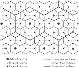
FIGURE 3.32 Diagram of a classic central place system (market areas: a K = 3 hierarchy). SOURCE: de Souza, 1990, p. 258.
Christaller understood the power of this model of an economic landscape (now referred to as an isotropic plane):
This model is “correct” in itself, even if it is never to be found in the reality of settlement landscape in pure form: mountain ranges, variable ground; but also variable density of population, variable income ratios and sociological structure of the population, historical developments and political realities bring about deviations from the pure model. (Christaller, 1972, p. 608)
In effect, the model allows Christaller to separate the signal (pattern) from the noise (deviations) and, at the same time, to offer explanations for both signal and noise. He also recognized the link between space and time, pattern and change:
I thus did not satisfy myself with setting up a model for an invariable and constant economic landscape (thus, for a static condition)—but instead I also tried to show how the number, size and distribution of the central places change, when the economic factors change…. (Christaller, 1972, p. 608)
The explanations were built on the concept of a central place. Christaller saw settlements of all sizes as serving functions (commercial, governmental, educational, recreational, medical, etc.) for themselves and for a surrounding population. To use this conceptual building block, Christaller had to find a way of measuring the quality of centrality, and to do so, he used the number of telephone connections as an indicator, scaled to the population size of the place. Here we can see echoes of his childhood preoccupation with “statistics.”
According to Christaller (1972, p. 609), given this connection indicator: “I was able to assign all central places in South Germany value indication numbers from 1 to 2825 (Munich).” After arraying the values into size classes: “I was able to mark in the central places in South Germany, according to their significance as central places, on a map, to measure the distances among them, and to determine their rank in the hierarchy of their ‘complementary areas’ which belonged to them (i.e., of their surrounding territory).”
At this point, the mapped patterns and the theoretical patterns intersect in a brilliant exercise in spatial thinking. Settlements are scaled by size—and therefore distance—classes, and these classes are organized into a hierarchy that captures size, number, spacing, and spatial arrangements. Different types of hierarchy arranged settlements on the basis of different logics of grouping and dependency: K-3 for efficiency or markets, K-4 for optimal traffic flows, and K-7 for efficiency of administration:
… the lowest ranked central places have a surrounding territory with a radius of 4–5 kilometers, and an average population of 3,000 (in the central place and surrounding territory) and their distances from the nearest central places, which according to the model lie within hexagonal (six-sided) connections, amount to seven kilometers. Within the completely regular hexagonal system of central places, the distances of all higher ranked central places can be derived, inasmuch as one multiplies the distance of the next lowest ranking central place by √3; the sequence of distances is thus: 7–12–21–36–62–108–185 … km. (Christaller, 1972, p. 609)
Christaller had explained the size, number, and distribution of settlements in one theoretical structure that has both an economic and a geographic rationale to it. It has both an algebraic and a geometrical interpretation. It is both static and dynamic. It is both abstract and concrete: “Thus, I was able to find surprising concurrences between geographical reality and the abstract schema of the central places (the theoretical model) especially in the predominantly agrarian areas of North and South Bavaria” (Christaller, 1972, p. 609).
The process of development of this intellectual structure also showed echoes of Christaller’s youth:
On Sundays, or also Saturday and Sunday, I used to hike around in the beautiful landscapes of
the Frankish Alps. While hiking, I mentally developed the progress of my work…. Thus, many an idea which helped me progress … gave me the happiness of a discoverer; it was connected in my memory to some forest path or other, just where I was, where the sun cast its light patches through the foliage onto the earth…. (Christaller, 1972, p. 609)
Christaller’s thinking was grounded in space, it was about space, and it was captured in spatial diagrams.
3.8.4 Walter Christaller as a Spatial Thinker
To many geographers in the decades between the 1950s and 1970s, Christaller’s work was an inspiration, a model to be applied literally and to be followed metaphorically. It was one of the cornerstones of the spatial analysis approach to geography. It was tested in many places, adapted, and rejected by some. It served as a planning tool in many parts of the world. For later generations of geographers, it became an emblem.
Whatever one’s judgment of the theory, the discovery itself was an extended exercise that shows the power and process of spatial thinking:
If I may very briefly once again describe my methodology: first of all play, paint on the maps, draw in lines and points, but in a very playful fashion—then problems suddenly emerge. Then I tried, while hiking, to elucidate them, to solve them, while hiking the thoughts are shaken back into their proper places. And, last of all, comes the completion and formulation. Thereby, the language should be of a sort that chimes, that is audible, and not just something for reading. In general, the opinion predominates that creative scholarly work is born at the desk. It must not be so. Mine was created while hiking, in nature. I, moreover, am glad to consider myself a geographer. (Christaller, 1972, p. 610)
As William Bunge (1966, p. 133) wrote: “With the possible exception of cartography, this author is of the opinion that the initial and growing beauty of central place theory is geography’s finest intellectual product and puts Christaller in a place of great honor.”
3.9 CONCLUSION
As the examples in this chapter illustrate, there are different levels of performance in spatial thinking as a function of age and experience, and there are different modes of performance in spatial thinking in different contexts. Marie Tharp and Walter Christaller exemplify the power of spatial thinking in the process of scientific discovery. Some geoscience students never seem to master the relations between dip and strike in rock formations. An air traffic controller may not be any more effective at assembling a child’s toy than an artist. A child who has learned to tie a shoelace may not yet be able to tie a necktie. For some of these activities, years of formal training are required. For others, learning is informal and unstructured.
There are three messages about the role of spatial thinking in everyday life, at work, and in science. The first is the pervasiveness, power, and flexibility of the process of spatial thinking: successful problem solving in many contexts depends to a significant degree upon spatial thinking. The second is the extent to which there are significant variations in how and how well the process is executed: there is no single “best” way of thinking spatially. The third is the importance of meeting the challenge of formal training in spatial thinking: workplace-relevant skills require considerable investment of individual and societal resources. Although some learning occurs informally, much depends upon the formal education system. Chapter 4 considers the teaching and learning of spatial thinking skills: How do people acquire the spatial knowledge, spatial ways of thinking and acting, and spatial capabilities that are increasingly important in an information technology-driven society and economy?


