
Appendix I
Cost-Effectiveness Analyses of Colorectal Cancer Screening: Results from a Pre-conference Modeling Exercise Michael Pignone, M.D., M.P.H.
SLIDE 1
SLIDE 1 NOTES: I would like to thank the following people for their work and advice on this exercise or on a previous review conducted for the US Preventive Services Task Force: Judy Wagner, Louise Russell, Martin Brown, Somnath Saha, Jeanne Mandelblatt, Tom Hoerger, Steve Teutsch, and all of the modelers who participated in this exercise.
SLIDE 2
SLIDE 2 NOTES: The aims of the pre-Workshop modeling exercise, as I see it, were two-fold: The first was to compare the several different cost-effectiveness analyses of colorectal cancer screening. Such a comparison has three motivations: to gain insight into reasons for different results; to determine areas for future research focus; and potentially to learn something about how different screening strategies stack up against one another. The last motivation, however, is less important than the first two.
The second objective is to use insights from this exercise to better inform future modeling and direct future CRC research efforts. The exercise should lead to better understanding of our parameters, better models, and an identification of questions or issues that need to be incorporated into the models.
SLIDE 3

SLIDE 3 NOTES: As with some other cancers, colorectal cancer is, of course, an important disease that is amenable to screening. However, unlike many conditions amenable to preventive interventions, there are several different screening tests available, each supported by its own body of evidence on effectiveness, risks and costs. In other areas of cancer screening there is usually one dominant modality. With CRC screening, several modalities are available.
Also, unlike many other areas, there are several recent high-quality published cost-effectiveness analyses which reached different conclusions about the relative merits of alternative screening strategies. That fact provides an interesting opportunity, because it offers us a chance to explore how that variation might arise, and whether the variation is there for good reasons, or whether we should try to reduce the variation through standardization of methods and assumptions.
SLIDE 4
SLIDE NOTES 4: A precursor to this exercise was the work my colleagues and I did for the US Preventive Services Task Force in 2000 (Pignone et al., 2002). At that time, we reviewed seven published models. All seven found that any of the main screening strategies for colorectal cancer were cost-effective compared with no screenings. The cost-effectiveness of any screening strategy compared with doing nothing was generally below $30,000 per year of life added across all models.
The models, however, did reach some different results as to the most effective and most cost-effective strategies. Some of those results were surprising to us.
We also concluded that the variations were likely due to differences and uncertainties in input parameters, but it was impossible to sort out these factors from the published studies. We called for an exercise similar to the one undertaken for this workshop.
SLIDE 5
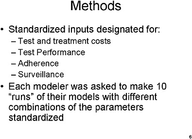
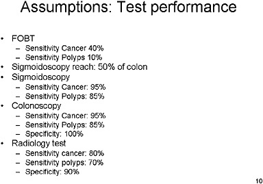
SLIDE 5 NOTES: Here is a brief description of the methods used in the pre-workshop modeling exercise.
Each modeler was asked to analyze 5 screening strategies, as well as no screening, as listed above.
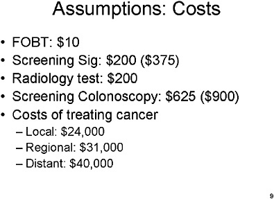
The prototype radiological screening test was defined to have characteristics somewhere in between barium enema, which is relatively inexpensive, and virtual colonoscopy, which is more sensitive but more expensive.
SLIDE 7
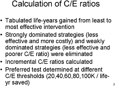
SLIDE 7 NOTES: For each run, we did the following: We ordered the years of life saved for every strategy from lowest to highest. We identified the strongly dominated strategies—those which were both less effective and more costly than at least one other strategy. Strongly dominated strategies were eliminated. Of the remaining strategies, we identified those that were weakly dominated—they were both less effective and their costs per year of life added were higher than at least one other strategy. The remaining strategies constitute the undominated set.
We then calculated the incremental cost-effectiveness ratio: the incremental costs per incremental year of life added by moving from the least (undominated) strategy to the next least (undominated) strategy, and so on.
We designated a “preferred strategy” for any cost-effectiveness limit as the one with the highest effectiveness (years of life added) whose incremental cost-effectiveness ratio meets a given limit.
SLIDE 12
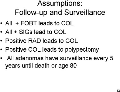
SLIDE 12 NOTES: All patients with positive FOBT tests would receive a follow-up colonoscopy.
All patients with positive sigmoidoscopy would receive a follow-up colonoscopy.
All patients with positive radiology test would receive a follow-up colonoscopy
All patients with a polyp found on colonoscopy screening would have the lesion removed as part of that procedure.
All patients with adenomas found on screening and removed in screening or followup would be entered into a surveillance program requiring a full colonoscopy every 5 years until death or until the patient reaches age 80.
SLIDE 13
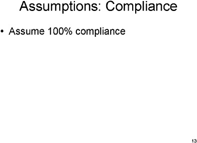
SLIDE 13 NOTES: When we standardized on assumptions about compliance, we asked modelers to assume that all individuals would be fully compliant with all screening, follow-up and surveillance tests. That assumption is a poor description of reality, but it provided a level playing field for all procedures.
SLIDE 14
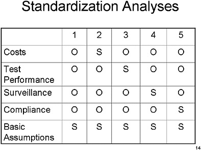
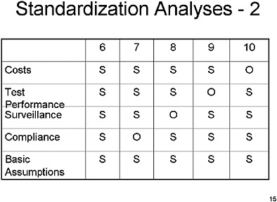
SLIDE 14 NOTE: In this and the next chart, the rows depict the different assumptions and the columns depict the specific run. “S” means that the parameters in a specific run and input group (for example, in run number 2, and the “Cost” assumptions) were set to the standardized values we specified. “O’ means that the parameters in a specific run and input group (for example, in run number 3 and the “Cost” assumptions) were set to the values in the modeler’s originally published or current version of the model.
Run number 1 represents the original assumptions across all four parameter areas.
SLIDE 16
SLIDE 16 NOTES: Now for the results of the exercise.
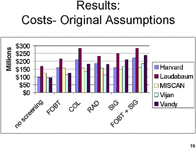
The current chart shows—for the original assumptions (Run 1)—the lifetime cost in a population of 100,000 50-year old individuals of screening, follow-up, surveillance and treatment of CRC in millions of dollars. That value is shown for each of the five screening strategies and no screening.
Within each screening test, there is fairly substantial variation under the original assumptions about the costs of screening.
SLIDE 17
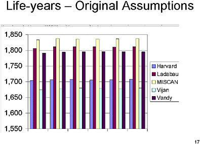
SLIDE 17 NOTES: This chart shows—for the original assumptions—the years of life lived in a population of 100,000 50-year old individuals.
Here, too, there is a substantial variation between the different models in terms of the number of years of life that would be generated through running the model under each of the different modelers’ assumptions.
SLIDE 18
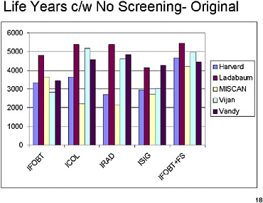
SLIDE 18 NOTES: This slide shows the years of life added, compared with the no-screening strategy, under the original assumptions (Run 1).
Although the metric has changed (from total number of years of life lived to additional years of life lived), the same pattern is replicated across the models. Substantial differences exist between models.
SLIDE 19
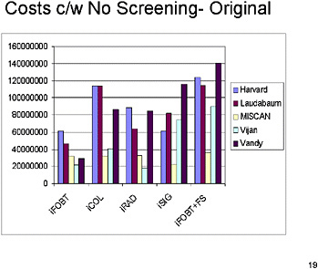
SLIDE 19 NOTES: This chart shows extra lifetime costs compared with the no-screening strategy, under the original assumptions (Run 1). Substantial differences in cost persist across models for each of the different screening strategies, a full colonoscopy every 5 years until death or until the patient reaches age 80.
SLIDE 20
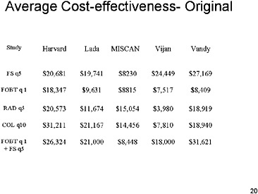
SLIDE 20 NOTES: Here are the average cost-effectiveness ratios under the original assumptions (Run 1). By average, I mean the ratio of additional costs to additional effectiveness when each strategy is compared with no screening.
A quick scan of these results shows that almost all of the strategies have cost-effectiveness ratios of less than $30,000, regardless of the model used. The cost-effectiveness ratios tend to vary between $10,000 and $30,000 both across screening strategies and across models.
SLIDE 21
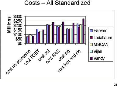
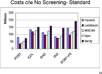
SLIDE 21 NOTES: This and subsequent slides provide results under the fully standardized assumptions (Run 6). All four parameter groups are standardized in this run.
The current slide shows—for the standardized assumptions (Run 6)—the lifetime cost of screening, follow-up, surveillance and treatment of CRC in millions of dollars. That value is shown for each of the five screening strategies and no screening.
Now there is much less variation across the models once assumptions have been standardized.
SLIDE 22
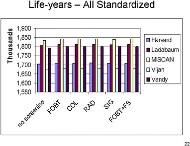
SLIDE 22 NOTES: This chart shows the years of life lived in a population of 100,000 50-year old individuals under the standardized assumptions.
Rough visual inspection suggests that there is probably a little less variation than there was under the original assumptions. Still, substantial variation exists in the number of years of life lived across models.
Interestingly, there appears to be more variation among the different models than there is among the different tests. These differences across models may reflect different assumptions about the natural history of CRC. Note that neither natural history nor model structure have been standardized.
SLIDE 24

SLIDE 24 NOTES: This slide shows the years of life added, compared with the no-screening strategy, under the standardized assumptions (Run 6). Variation across models is now somewhat reduced, probably because some of the differences in assumptions about natural history wash out when the metric is years of life added compared with no screening. Nevertheless, substantial differences remain across models.
SLIDE 25
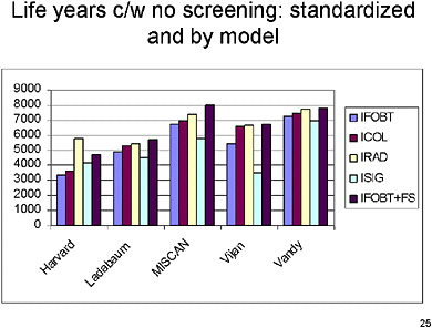
SLIDE 25 NOTES: In this chart and the next, the same results are grouped by model instead of by strategy. You can see that there is some variation in terms of life years saved within each model by the different strategies, suggesting that the strategies have different levels of effectiveness.
SLIDE 26
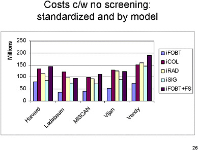
SLIDE 26 NOTES: This slide groups lifetime costs by model. There are now some differences across strategies for all models, but they are relatively small across different tests, with FOBT generally less costly in each model than the other screening strategies. The relative costs across strategies tend to follow pretty much the same pattern across the different models.
SLIDE 27
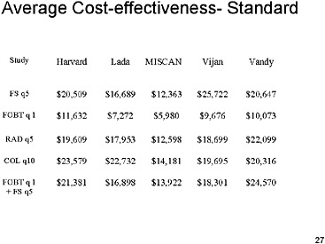
SLIDE 27 NOTES: Here is the average cost-effectiveness under the standardized assumptions (Run 6). The results are quite similar to what was seen under the original assumptions for average cost-effectiveness. The results here vary from about $6,000 per life-year saved to about $25,000 per life-year saved. It appears from visual inspection that there is slightly less overall variation than we had under the original assumptions.
SLIDE 28

SLIDE 28 NOTES: The rest of this presentation is about incremental cost-effectiveness ratios (as opposed to average cost-effectiveness ratios) and preferred strategies.
Recall that the incremental cost-effectiveness ratio (ICER) is calculated by eliminating all strongly and weakly dominated strategies and then sorting the remaining strategies in ascending order according to years of life added compared with no screening. The incremental ratio is calculated for each strategy as the extra costs incurred per extra year of life added by moving from each strategy to the next most effective strategy.
SLIDE 29
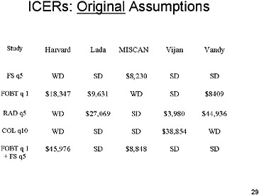
SLIDE 29 NOTES: Here are the ICERs under the original assumptions (Run 1). There are definite differences across models in which strategies are dominated and which are not.
For example, flexible sigmoidoscopy every five years is dominated in all but the Miscan model.
In four of the five models, colonoscopy is either weakly or strongly dominated by other tests. In the Vijan model it has a cost-effectiveness ratio of $38,000 per year of life added.
SLIDE 30
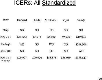
SLIDE 30 NOTES: This chart shows the ICER’s under the standardized assumptions (Run 6). With assumptions standardized, the first four models get very similar results. Under the specific set of standardized assumptions made about each strategy, FOBT screening generally had ICER’s between $5,000 and $12,000 per year of life saved, while flexible sigmoidoscopy every five years was dominated in all models.
Radiology and colonoscopy were dominated in most models. When they were not, they had a high incremental cost-effectiveness ratio.
Finally, annual FOBT plus flexible sigmoidoscopy under these particular standardized assumptions produced additional life years at a fairly high additional cost. The highest estimate was from the Vanderbilt model, with over $350,000 per additional life year saved. Those results merit more discussion.
SLIDE 31
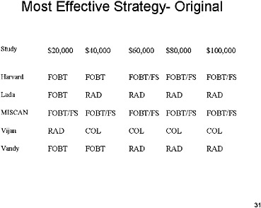
SLIDE 31 NOTES: This slide shows—for the original assumptions—the most effective strategy (i.e., the strategy that produces the largest number of additional years of life among all non-dominated strategies) under given incremental cost-effectiveness thresholds. So, for example, the Harvard model predicts that annual FOBT is the most effective strategy among all strategies whose ICER is $20,000 or less.
There is a great deal of variation across models in which strategy is preferred at any cost-effectiveness threshold.
SLIDE 32

SLIDE 32 NOTES: This chart is the same as the previous chart, except that the assumptions are fully standardized (Run 6). Here, almost all of the differences across models disappear. The most effective strategy at any different threshold is the same. In fact, the only difference is the threshold level at which the FOBT with FSIG overtakes FOBT alone as the preferred strategy.
SLIDE 33

SLIDE 33 NOTES: This exercise had several limitations. Some were a function of the limited time we had to design and conduct the exercise and the amount of effort that the modelers could realistically expect to make to support the exercise.
The exercise did not examine the effect of different assumptions about the natural history of colorectal cancers.
The modelers were provided with only one set of standard values for assumptions. Those standard values were not all realistic; many were selected because they would require the least amount of model redesign. True values of such parameters might be quite different, and another exercise would be warranted for such parameters.
The effects of standardizing assumptions might differ with other sets of screening strategies. It might be useful, for example, to do an exercise that includes more complex screening strategies such as one that begins with one screening test and transitions over time to another as individuals age.
Finally, there was no accounting for uncertainty in estimates. There is a method of doing sensitivity analysis, and we did not do Monte Carlo simulations to generate confidence intervals around some of our parameters. So we are dealing with point estimates here.
SLIDE 34

SLIDE 34 NOTES: In this chart and the next, the same results are grouped by model instead of by strategy. You can see that there is some variation in terms of life years saved within each model by the different strategies, suggesting that the strategies have different levels of effectiveness.
SLIDE 35
SLIDE 35 NOTES: Here are some preliminary thoughts about implications of this exercise. First, it would certainly be a good idea to establish some standard cost inputs, to eliminate this major source of variation across models.
We also need additional research in modeling compliance. I believe we are still missing some of the key input parameters that would help us to more effectively and accurately model what actually happens in terms of compliance.
Finally, I would like to see this process be applied in a number of different health areas. This kind of exercise can teach us a great deal, and I hope that this can be a model for future meetings or group projects. Not only can we understand better why results differ, but we may also advance the field of modeling itself.
REFERENCES
Ness RM, Holmes A, Klein R, Greene J, Dittus R. 1998. Outcome states of colorectal cancer: Identification and description using patient focus groups. Am J Gastroenterol 93(9):1491–1497 .
Pignone M, Saha S, Hoerger T, Mandelblatt J. 2002. Cost-effectiveness analyses of colorectal cancer screening: a systematic review for the U.S. Preventive Services Task Force. Ann Intern Med. 137(2):96–104.


