
Appendixes D-Q
Introduction
Appendixes D-Q contain the slide presentations of 14 speakers who were invited to address the workshop on specific topics. The presentations are reprinted here as they were presented to workshop participants, with little editing except format changes to permit printing and the addition of text summarizing accompanying remarks or clarification not shown on the slide. The original PowerPoint presentations are available on the Institute of Medicine website at http://www.iom.edu/crcworkshop.
Appendix D
Overview of Harvard Model Karen M.Kuntz, ScD.
SLIDE 1
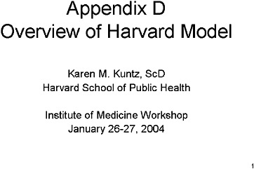
SLIDE 1 NOTES: The “Harvard Model” described here is the one presented in Frazier and colleagues (Frazier et al., 2000). That model was used to produce the results of the Pre-workshop Exercise described elsewhere in the workshop summary.
SLIDE 2
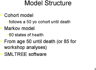
SLIDE 2 NOTES: The model is a Markov design, programmed in SMLTREE™, a decision analysis software package. It follows a cohort of 50-year-old persons until death. (For the pre-workshop exercise, individuals were followed through age 85.) Sixty states of health track different underlying disease states, such as whether a person has a low-risk or high-risk polyp, and the location of that polyp, whether there is an undiagnosed or diagnosed cancer, and the stage of that diagnosis.
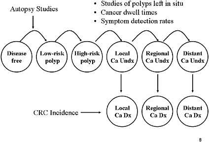
SLIDE 3
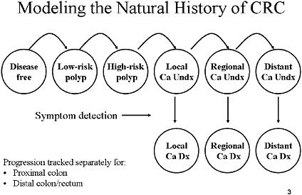
SLIDE 3 NOTES: This slide lays out a very simple diagram of the various states of health in which an individual can reside. Some states of health are free of any polyps or cancer in the colorectal tract. Each year there is a chance that a polyp will develop. Polyps then can progress to undiagnosed cancer. Cancers are staged using the NCI SEER nomenclature: localized, regional and distant. Every year, there is a chance that a cancer will be diagnosed as a result of symptoms. The probability of such detection varies with the stage of the patient.
The progression described above is tracked separately for the distal and proximal colon. Thus, the model can determine whether a particular polyp or cancer is in the part of the colorectal tract that is reachable by sigmoidoscopy. We assumed that all cancers arise from polyps, but not all polyps are destined to become cancers.
Definitions: Low-risk polyp=an adenomatous polyp smaller than 10 cm and with tubular histology. High-risk polyp=an adenoma greater than or equal to 1 cm or containing villous histology. Ca=cancer. Undx=undiagnosed. Dx=diagnosed.
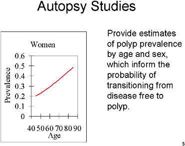
SLIDE 4
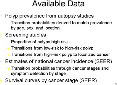
SLIDE NOTES 4: We estimated age- and sex-specific prevalence of adenomatous polyps using a weighted logistic regression analysis of results from 6 autopsy studies. We then derived transition probabilities to low-risk adenoma such that the model reproduced the age- and sex-specific prevalence.
Polyps were distributed across proximal colon, distal colon/rectum, or both sites based on data from autopsy studies and screening studies. We used screening studies to estimate the proportion of adenomas that are high risk.
The transition probability from low-risk to high-risk adenoma was estimated from studies of small polyps left in situ and reexamined annually. The transition probability from high-risk adenoma to invasive localized cancer was estimated from a study of patients who refused resection of high-risk polyp.
We varied the estimates of cancer progression and symptom detection across clinically plausible ranges so that the stage distribution and cancer incidence was similar to those reported by the National Cancer Institute’s SEER system.
SLIDE 6
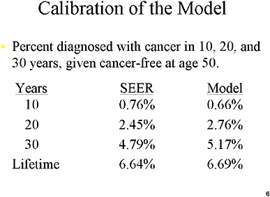
SLIDE 6 NOTES: We adjusted the transition probabilities from normal status to polyps, from polyps to undiagnosed cancer, and from undiagnosed to diagnosed caner until we achieved reasonable agreement with available data on cancer incidence. To do this, we used DevCan, a feature of the NCI SEER database which estimates the probability of developing cancer in one’s lifetime. We used DevCan data from the late 1970’s to predict cancer rates for a population that would not routinely receive screening. (Probabilities for recent years have most likely been affected by the rapid increase in the utilization of colorectal screening tests)
Here is an example of how our resulting model performed in predicting cancers in a cohort of men who were cancer free at age 50.
How close is close enough? At the time we published our paper, we used informal comparisons (i.e., the model predictions and the SEER predictions were “reasonably” close by visual inspection). Today, we are in the process of developing more sophisticated techniques, specifically statistical likelihood-based techniques to calibrate our models. Those improvements are not reflected in the modeling exercise we undertook for this workshop.
SLIDE 7
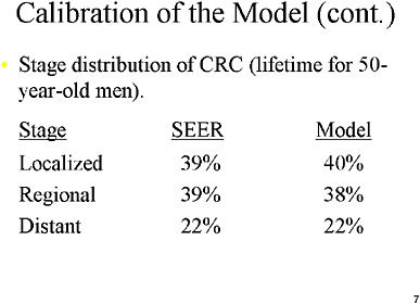
SLIDE 7 NOTES: We also calibrated the stage-distributions predicted in the model (in the absence of screening) with stage distributions reported in the NCI SEER database. We used data from the few studies that followed the progression of polyps not removed on first detection, estimates of the dwelling time of cancer by stage, estimates of symptom detection rates, to guide our initial model assumptions, and we ultimately adjusted those assumptions to reach reasonable agreement with the SEER data.
SLIDE 9
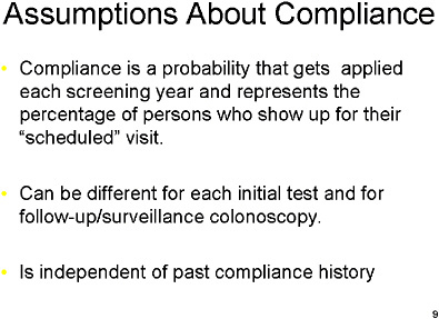
SLIDE 9 NOTES: For example, if a screening strategy involves an annual FOBT test, and if we are assuming a 60 percent compliance rate, then each individual has a 60 percent chance of actually getting an FOBT in each year. The compliance in any particular year is independent of past compliance history.
We also assume that the compliance rate might differ for each screening technology and for follow-up colonoscopies. For example, the compliance rate could be 60 percent for FOBT, but 80 percent for colonoscopy scheduled following a positive screen.
SLIDE 10
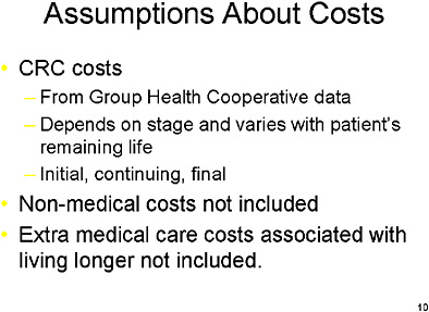
SLIDE 10 NOTES: The source of screening procedure and CRC treatment costs was the Group Health Cooperative of Puget Sound (Taplin et al., 1995a; Taplin et al., 1995b). That study reported on the net costs of the initial treatment for CRC, a monthly cost of continuing care, and a final cost associated with the last year in which the patient lives. Thus, the longer a patient lives, the more CRC treatment costs he or she will incur. Procedure costs were obtained from the same source through personal communication.
We did not include non-medical costs or the extra medical care costs associated with living longer.
SLIDE 11
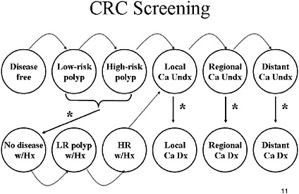
SLIDE 11 NOTES: To model a screening strategy, we superimposed a screening mechanism on the natural history model (the effects of screening are indicated by the asterisks). We modeled a screening, follow-up and surveillance strategy as follows: If a person has an underlying polyp and is screened, there is a chance (based on the sensitivity of the test) that the polyp will be found and removed. The person is now “disease free” but the model keeps track of whether that person had a low-risk or high-risk polyp (as indicated by “w/Hx”). Those with high-risk polyps can be entered into a surveillance protocol consisting of periodic colonoscopy. For the pre-workshop exercise, however, all individuals with polyps were assumed to undergo periodic surveillance. If a person has undiagnosed cancer and is screened, there is a chance that the cancer will become detected.
We assumed that recurrence rates of low-risk polyps after polypectomy were higher for individuals with a history of a high-risk polyp diagnosis compared with a prior diagnosis of low-risk polyp and that the risk was higher in the first year following polyp removal compared with subsequent years.
SLIDE 12
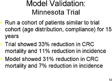
SLIDE 12 NOTE: We validated the model against the results of the Minnesota trial of bi-annual FOBT (Mandel et al., 1999; Mandel et al., 2000). We entered a cohort of patients similar to those who participated in the trial and used the compliance rates observed in that trial. We ran our model for 15 years, the duration of the Minnesota trial. The screened individuals in the trial showed a 33 percent reduction in cancer mortality and an 11 percent reduction in cancer incidence. In comparison, our model showed a 31 percent reduction in cancer mortality and a 7 percent reduction in incidence. So, our model was reasonably consistent with the results of that trial.
SLIDE 13
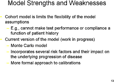
SLIDE 13 NOTES: The model presented here has certain limitations that restrict our flexibility in altering model assumptions. It is difficult with a Markov structure to maintain detailed information on each individual’s history over time, because each additional piece of information requires another set of health states, and the number of health states quickly multiplies. For example, it would be prohibitively complex to make test performance or compliance a function of patient history.
We are currently testing a new version, which is a Monte Carlo design. In such models, it is easy to keep each patient’s history as he or she ages. The new model also incorporates eight new risk factors which alters the underlying progression of disease.
Finally, we are taking a more formal approach to calibrating our model assumptions. We are using statistical maximum likelihood methods to optimize our natural history assumptions.
The new model is a precursor to one of several collaborating as part of the NCI’s CISNET program, which is discussed in Dr. Rocky Feuer’s presentation later in this workshop.
REFERENCES
Frazier AL, Colditz GA, Fuchs CS, Kuntz KM. 2000. Cost-effectiveness of screening for colorectal cancer in the general population. JAMA. 284(15):1954–1961.
Mandel JS, Church TR, Bond JH, Ederer F, Geisser MS, Mongin SJ, Snover DC, Schuman LM. 2000. The effect of fecal occult-blood screening on the incidence of colorectal cancer. N Engl J Med. 343(22):1603–1607.
Mandel JS, Church TR, Ederer F, Bond JH. 1999. Colorectal cancer mortality: Effectiveness of biennial screening for fecal occult blood. J Natl Cancer Inst. 91(5):434–437.
Taplin SH, Barlow W, Urban N. 1995a. Erratum: Stage, age, comorbidity, and direct costs of colon, prostate, and breast cancer care. J Natl Cancer Inst. 87(8):610.
Taplin SH, Barlow W, Urban N, Mandelson MT, Timlin DJ, Ichikawa L, Nefcy P. 1995b. Stage, age, comorbidity, and direct costs of colon, prostate, and breast cancer care. J Natl Cancer Inst. 87(6):417–426.


