
12
Estimating Cancer Risk
INTRODUCTION
This chapter presents models that allow one to estimate the lifetime risk of cancer resulting from any specified dose of ionizing radiation and applies these models to example exposure scenarios for the U.S. population. Models are developed for estimating lifetime risks of cancer incidence and mortality and take account of sex, age at exposure, dose rate, and other factors. Estimates are given for all solid cancers, leukemia, and cancers of several specific sites. Like previous BEIR reports addressing low-LET (linear energy transfer) radiation, risk models are based primarily from data on Japanese atomic bomb survivors. However, the vast literature on both medically exposed persons and nuclear workers exposed at relatively low doses has been reviewed to evaluate whether findings from these studies are compatible with A-bomb survivor-based models. In many cases, results of fitting models similar to those in this chapter have been published.
Risk estimates are subject to several sources of uncertainty due to inherent limitations in epidemiologic data and in our understanding of exactly how radiation exposure increases the risk of cancer. In addition to statistical uncertainty, the populations and exposures for which risk estimates are needed nearly always differ from those for whom epidemiologic data are available. This means that assumptions are required, many of which involve considerable uncertainty. Risk may depend on the type of cancer, the magnitude of the dose, the quality of the radiation, the dose-rate, the age and sex of the person exposed, exposure to other carcinogens such as tobacco, and other characteristics of the exposed individual. Despite the abundance of epidemiologic and experimental data on the health effects of exposure to radiation, data are not adequate to quantify these dependencies precisely. Uncertainties in the BEIR VII risk models are discussed, and a quantitative assessment of selected sources of uncertainty is made.
In recent years, several national and international organizations have developed models for estimating cancer risk from exposure to low levels of low-LET ionizing radiation. These include the work of the BEIR V committee (NRC 1990), the International Commission on Radiological Protection (ICRP 1991), the National Council on Radiation Protection and Measurements (NCRP 1993), the Environmental Protection Agency (EPA 1994, 1999), the United Nations Scientific Committee on the Effects of Atomic Radiation (UNSCEAR 2000b), and the National Institutes of Health (NIH 2003). The approaches used in these past assessments are described in Annex 12A.
DATA EVALUATED FOR BEIR VII MODELS
As in earlier BEIR reports addressing health effects from exposure to low-LET radiation, the committee’s models for risk estimation are based primarily on the Life Span Study (LSS) cohort of survivors of the atomic bombings in Hiroshima and Nagasaki. As discussed in Chapter 6, the LSS cohort offers several advantages for developing quantitative estimates of risk from exposure to ionizing radiation. These include its large size, the inclusion of both sexes and all ages, a wide range of doses that have been estimated for individual subjects, and high-quality mortality and cancer incidence data. In addition, because the exposure was to the whole body, the LSS cohort offers the opportunity to assess risks for cancers of a large number of specific sites and to evaluate the comparability of site-specific risks.
Another consideration in the choice of data was that it was considered essential that the data used by the committee eventually be available to other investigators. The Radiation Effects Research Foundation (RERF) has developed a policy of making summarized data available to those who request it, thus enabling other investigators to analyze data used by the BEIR VII committee. This is not the case for data sets on most other radiation-exposed cohorts.
Although the committee’s models have been developed from A-bomb survivor data, attention has been given to their compatibility with data from other cohorts. Fortunately, for
most cohorts with suitable data for developing quantitative risk models, analyses based on models similar to those used by the committee have been conducted and published. This facilitated the committee’s evaluation of data from other studies. Pooled analyses of thyroid cancer risks (Ron and others 1995a) and of breast cancer risks (Preston and others 2002a) were especially helpful in this regard, as were several meta-analyses by Little and colleagues. In addition, the many published analyses based on A-bomb survivor data have guided and facilitated the committee’s efforts in its choice of models. The committee notes particularly the main publications on mortality (Preston and others 2003) and incidence data (Thompson and others 1994) and the models developed by UNSCEAR (2000b) and NIH (2003).
The use of data on persons exposed at low doses and low dose rates merits special mention. Of these studies, the most promising for quantitative risk assessment are the studies of nuclear workers who have been monitored for radiation exposure through the use of personal dosimeters. These studies, which are reviewed in Chapter 8, were not used as the primary source of data for risk modeling principally because of the imprecision of the risk estimates obtained. For example, in a large combined study of nuclear workers in three countries, the estimated relative risk per gray (ERR/Gy) for all cancers other than leukemia was negative, and the confidence interval included negative values and values larger than estimates based on A-bomb survivors (Cardis and others 1995).
Since the publication of BEIR V, data on cancer incidence in the LSS cohort from the Hiroshima Tumor Registry have become available, whereas previously only data from the Nagasaki Tumor Registry were available. Thus, the committee could use both incidence and mortality data to develop its models. The incidence data offer the advantages of including nonfatal cancers and of better diagnostic accuracy. However, the mortality data offer the advantages of covering a longer period (1950–2000) than the incidence data (1958–1998) and of including deaths of LSS members who migrated from Hiroshima and Nagasaki to other parts of Japan.
MEASURES OF RISK AND CHOICE OF CANCER END POINTS
To express the health impact of whole-body exposures to radiation, the lifetime risk of total cancer, without distinction as to site, is usually of primary concern. Estimates of risk for both mortality and incidence are of interest, the former because it is the most serious consequence of exposure to radiation and the latter because it reflects public health impact more fully. The time or age of cancer occurrence is also of interest, and for this reason, estimates of cancer mortality risks are sometimes accompanied by estimates of the years of life lost or years of life lost per death. Because leukemia exhibits markedly different patterns of risk with time since exposure and other variables, and also because the excess relative risk for leukemia is clearly greater than that for solid cancers, all recent risk assessments have provided separate models and estimates for leukemia.
For exposure scenarios in which various tissues of the body receive substantially different doses, estimates of risks for cancers of specific sites are needed. Adjudication of compensation claims for possible radiation-related cancer, which is usually specific to organ site, also requires site-specific estimates. Furthermore, site-specific cancers vary in their causes and baseline risks, and it might thus be expected that models for estimating excess risks from radiation exposure could also vary by site. For this reason, even for estimating total cancer risk, it is desirable to estimate risks for each of several specific cancer sites and then sum the results.
The development of site-specific models is limited by data characteristics. For A-bomb survivor data on solid cancers, parameter estimates based on site-specific data are less precise than those based on all solid cancers analyzed as a group, particularly for less common cancers. It is especially difficult to detect and quantify the modifying effects of variables such as sex, age at exposure, and attained age for site-specific cancers. It was for these reasons that the BEIR V committee provided estimates for only five broad cancer categories.
In addition to statistical uncertainties, it has recently been recognized that estimates of the modifying effects of age at exposure based on A-bomb survivor data can be influenced strongly by secular trends in Japanese baseline rates (Pierce 2002; Preston and others 2003). This occurs because age at exposure in the LSS cohort is confounded with birth cohort, making it impossible to estimate their separate effects without additional information on the relation of baseline and radiation-related risks. (See Annex 12B for further discussion of this issue.) Japanese rates for several cancer sites changed over the period 1950–1998 as Japan became more Westernized, including rates for cancers of the stomach, colon, lung, and female breast. A related problem is that baseline risks for the United States and Japan differ substantially for many cancer sites, and it is unclear how to account for these differences in applying models developed from A-bomb survivor data to estimate risks for the U.S. population.
Pierce and colleagues (1996) and, more recently, Preston and colleagues (2003) found little evidence of heterogeneity among excess relative risk (ERR)1 models developed for several specific cancer sites. Although these authors caution that this finding should be taken mainly as a warning against overinterpreting apparent differences in sites, some grouping of cancers seems justified. In developing its models, the committee has tried to strike a balance between allowing for differences among cancer sites and statistical precision. As discussed later in this chapter, most of the committee’s mod-
els for site-specific cancers make use of data on all solid cancers to estimate the modifying effects of age at exposure and attained age, but make use only of data for the site of interest to estimate the overall level of risk.
Considerations in deciding on the sites for which individual estimates should be provided are whether or not the cancer has been linked clearly with radiation exposure and the adequacy of the data for developing reliable risk estimates. On the first point, it can be argued that the range of uncertainty for risk of a particular cancer is of interest regardless of whether or not a statistically significant dose-response had been observed, a position taken by NIH (2003). Cancers of the salivary glands, stomach, colon, liver, lung, breast, bladder, ovary, and thyroid and nonmelanoma skin cancer have all been linked clearly with radiation exposure in A-bomb survivor data, with evidence somewhat more equivocal for a few additional sites such as esophagus, gall bladder, and kidney. Other studies support many of these associations, and bone cancer has been linked with exposure to α-irradiation from 224Ra. Leukemia has been strongly linked with radiation exposure in several studies including those of atomic bomb survivors.
Another consideration in selecting sites for evaluation is the likelihood of exposure scenarios that will irradiate the site selectively. Here it is noted that inhalation exposures will selectively irradiate the lung, exposures from ingestion will selectively irradiate the digestive organs, exposure to strontium selectively irradiates the bone marrow, and exposure to uranium selectively irradiates the kidney.
Based on these considerations, the committee has provided models and mortality and incidence estimates for cancers of the stomach, colon, liver, lung, female breast, prostate, uterus, ovary, bladder, and all other solid cancers. Incidence estimates are also provided for thyroid cancer.
The inclusion of cancers of the prostate and uterus merits comment because these cancers are not usually thought to be radiation-induced and have not been evaluated separately in previous risk assessments. However, the committee did not want to include these cancers in the residual category of “all other solid cancers,” particularly since prostate cancer is much more common in the United States than in Japan.
THE BEIR VII COMMITTEE’S PREFERRED MODELS
Approach to Analyses
This section describes the results of analyses of data on cancer incidence and mortality in the LSS cohort that were conducted by the committee with the help of RERF personnel acting as agents of the National Academies. Analyses of cancer incidence were based on cases diagnosed in the period 1958–1998. Analyses of cancer mortality from all solid cancers and from leukemia were based on deaths occurring in the period 1950–2000 (Preston and others 2004), whereas analyses of mortality from cancer of specific sites were based on deaths occurring in the period 1950–1997 (Preston and others 2003). Both excess relative risk models and excess absolute risk (EAR)2 models were evaluated. Methods were generally similar to those that have been used in recent reports by RERF investigators (Pierce and others 1996; Preston and others 2003) and were based on Poisson regression using the AMFIT module of the software package EPICURE (Preston and others 1991). Additional detail is given in Annex 12B.
All analyses were based on the newly implemented DS02 dose estimates. Doses were expressed in sieverts, with a constant weighting factor of 10 for the neutron dose; that is, the doses were calculated as γ-ray absorbed dose (Gy) + 10 × neutron absorbed dose (Gy). The DS02 system provides estimates of doses to several organs of the body. For site-specific estimates, the committee used dose to the organ being evaluated, with colon dose used for the residual category of “other” cancers. The weighted dose, d, to the colon was used for the combined category of all solid cancer or all solid cancers excluding thyroid and nonmelanoma skin cancer. Additional discussion of the doses used in the analyses is given in Annex 12B.
Models for All Solid Cancers
Risk estimates for all solid cancers were obtained by summing the estimates for cancers of specific sites. However, the general form of the model and the estimates of the parameters that quantify the modifying effects of age at exposure and attained age were (with some exceptions) based on analyses of data on all solid cancers. Such analyses offer the advantage of larger numbers of cancer cases and deaths, which increases statistical precision.
As discussed in Chapter 6, most recent analyses of data on the LSS cohort have been based on either ERR models, in which the excess risk is expressed relative to the background risk, or EAR models, in which the excess risk is expressed as the difference in the total risk and the background risk. With linear dose-response functions, the general models for the ERR and EAR are given below:
or
where λ(c, s, a, b) denotes the background rate at zero dose, and depends on city (c), sex (s), attained age (a), and birth cohort (b). The terms βs ERR(e, a) and βs EAR(e, a) are, respectively, the ERR and the EAR per unit of dose expressed in sieverts, which may depend on sex (s), age at exposure (e), and attained age (a).
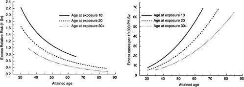
FIGURE 12-1A Age-time patterns in radiation-associated risks for solid cancer incidence excluding thyroid and nonmelanoma skin cancer. Curves are sex-averaged estimates of the risk at 1 Sv for people exposed at age 10 (solid lines), age 20 (dashed lines), and age 30 or more (dotted lines). Estimates were computed using the parameter estimates shown in Table 12-1.
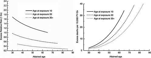
FIGURE 12-1B Age-time patterns in the radiation-associated risks for all solid cancer mortality. Curves are sex-averaged estimates of the risk at 1 Sv for people exposed at age 10 (solid lines), age 20 (dashed lines), and age 30 or more (dotted lines). Estimates were computed using the parameter estimates shown in Table 12-1.
The most recent analyses of A-bomb survivor cancer incidence and mortality data (e.g., Preston and others 2003, 2004) are based on models in which ERR (e, a) and EAR (e, a) are of the form below:
(12-1)
The parameters γ and η quantify the dependence of the ERR or EAR on e and a. These models, with dependence on both age at exposure and attained age, were chosen because of difficulties in distinguishing the fits of models with only one of those variables and because, with the incidence data, analyses of all solid cancers indicated dependence on both variables.
The committee’s models were developed from analyses of both LSS incidence and LSS mortality data. Analyses of incidence data were based on the category consisting of all solid cancers excluding thyroid and nonmelanoma skin cancers. These exclusions were made because both thyroid cancer and nonmelanoma skin cancer exhibit exceptionally strong age-at-exposure dependencies that do not seem typi-
cal of cancer of other sites (Thompson and others 1994). Because the most recent mortality data (1950–2000) available to the committee did not include site-specific solid cancers and because thyroid cancer and nonmelanoma skin cancer are rarely fatal, analyses of mortality data were based on the category of all solid cancers. The committee’s preferred models for estimating solid cancer risks are similar to the RERF model, except that the ERR and EAR depend on age at exposure only for exposure ages under 30 years and are constant for exposure ages over 30. That is,
(12-2)
where e is age at exposure in years, e* is equal to e − 30 when e < 30, and equal to zero when e 30, and a is attained age in years.
Figure 12-1A shows plots of the ERR and EAR for incidence of all solid cancers excluding thyroid cancer and nonmelanoma skin cancer as a function of exposure age and attained age using the BEIR VII model. Figure 12-1B shows similar plots for mortality from all solid cancers. Although the ERR and EAR models have the same form, the values and interpretation of the parameters are different. In particular, the ERR shows a decrease with attained age, whereas the EAR shows a strong increase with attained age. Both the ERR and the EAR decrease with increasing age at exposure for those exposed under age 30.
The committee chose the model shown in Equation (122) because it fitted both incidence and mortality data on all solid cancers excluding thyroid cancer and nonmelanoma skin cancer slightly better than the RERF model shown in Equation (12-1). There was no indication of a continued decrease with exposure age in the ERR or EAR after exposure age 30, and there was even a suggestion of an increase at older ages. Further discussion of the rationale for choosing the Equation (12-2) model, including a detailed description of analyses that were conducted by the committee, can be found in Annex 12B. In that annex, the committee evaluates several alternative model choices, including models that allow for dependence on age at exposure alone, on attained age alone, and on time since exposure instead of attained age. Also evaluated are models that use different functional forms to express the dependence on exposure age, attained age, or time since exposure. Although several alternative models provided reasonable descriptions of the data, the BEIR VII preferred model shown in Equation (12-2) provided the best fit.
Table 12-1 shows estimates of the parameters of the ERR and EAR models obtained from analyses of LSS incidence data (1958–1998) for all solid cancers excluding thyroid and nonmelanoma skin cancers and of LSS mortality data (1950–2000) for all solid cancers. Further description of these results and how they were obtained can be found in Annex 12B.
TABLE 12-1 ERR and EAR Models for Estimating Incidence of All Solid Cancers Excluding Thyroid and Nonmelanoma Skin Cancers and Mortality from All Solid Cancersa,b
|
ERR Models |
No. of Cases or Deaths |
ERR/Sv (95% CI) at Age 30 and Attained Age 60 |
Per-Decade Increase in Age at Exposure Over the Range 0–30 Yearsc (95% CI), γ |
Exponent of Attained Age (95% CI), η |
|
|
Males (βM) |
Females (βF) |
||||
|
Incidenced |
12,778 |
0.33 (0.24, 0.47) |
0.57 (0.44, 0.74) |
−0.30 (−0.51, −0.10) |
−1.4 (−2.2, −0.7) |
|
Mortalitye |
10,127 |
0.23 (0.15, 0.36) |
0.47 (0.34, 0.65) |
−0.56 (−0.80, −0.32) |
−0.67 (−1.6, 0.26) |
|
EAR Models |
|
EAR per 104 PY-Sv (95% CI) |
|
||
|
Males (βM) |
Females (βF) |
||||
|
Incidenced |
12,778 |
22 (15, 30) |
28 (22, 36) |
−0.41 (−0.59, −0.22) |
2.8 (2.15, 3.41) |
|
Mortalitye |
10,127 |
11 (7.5, 17) |
13 (9.8, 18) |
−0.37 (−0.59, −0.15) |
3.5 (2.71, 4.28) |
|
NOTE: Estimated parameters with 95% CIs. PY = person-years. aThe ERR or EAR is of the form βsD exp (γe*) (a / 60)η, where D is the dose (Sv), e is age at exposure (years), e* is (e − 30) / 10 for e < 30 and zero for e 30, and a is attained age (years). bThe committee’s preferred estimates of risks from all solid cancers are obtained as sums of estimates based on models for site-specific cancers (see Table 12-2 and text). cChange in ERR/Sv or EAR per 104 PY-Sv (per-decade increase in age at exposure) is obtained as 1 − exp (γ ). dBased on analyses of LSS incidence data 1958–1998 for all solid cancers excluding thyroid and nonmelanoma skin cancer. eBased on analyses of LSS mortality data 1950–2000 for all solid cancers. |
|||||
Models for Site-Specific Solid Cancers Other Than Breast and Thyroid
Although the committee provides risk estimates for both cancer incidence and mortality, models for site-specific cancers were based on cancer incidence data. This was done primarily because site-specific cancer incidence data are based on diagnostic information that is more detailed and accurate than death certificate data and because, for several sites, the number of incident cases is considerably larger than the number of deaths (see annex Table 12B-2). However, models developed from incidence data were checked for consistency with mortality data. Since there is little evidence that radiation-induced cancers are more rapidly fatal than cancer that occurs for other reasons, ERR models based on incidence data can be used directly to estimate risks of cancer mortality, whereas EAR models require adjustment. (See “Method of Calculating Lifetime Risks” for a description of how the models are used to estimate risks of cancer incidence and mortality.)
Models for estimating risks of solid cancers of specific sites other than breast and thyroid were also of the form shown in Equation (12-2). The committee’s approach to quantifying the parameters γ and η was to use the estimates obtained from analyzing incidence data on all solid cancers excluding thyroid and nonmelanoma skin cancers (shown in Table 12-1) unless site-specific analyses indicated significant departure from these estimates. This approach is similar to that used by UNSCEAR (2000b) except that the committee estimated the parameters βM and βF separately for each site of interest.
The committee’s preferred ERR and EAR models for site-specific cancer incidence and mortality are shown in Table 12-2. The estimates of βM and βF are for a person exposed at age 30 or older at an attained age of 60. Models for breast and thyroid cancer were based on published analyses that included data on medically exposed persons as discussed in the next two sections. For other sites, common values of the parameter γ indicating dependence on age at exposure could be used in all cases. With the ERR models, common values of the parameter indicating the dependence of risks on attained age (η) could be used in all cases except the category “all other solid cancers.” With the EAR models, it was necessary to estimate the attained-age parameter, η, separately for cancers of the liver, lung, and bladder, which may reflect variation in the pattern of increase with age for site-specific baseline rates.
The committee emphasizes that there is considerable uncertainty in models for site-specific cancers. Statistical uncertainty in the estimates of the main effect parameter βs is
TABLE 12-2 Committee’s Preferred ERR and EAR Models for Estimating Site-Specific Solid Cancer Incidence and Mortalitya
Cancer Site | No. of Cases | ERR Models | EAR Models | ||||||
βMb (95% CI) | βFb (95% CI) | γc | ηd | βMe (95% CI) | βFe (95% CI) | γc | ηd | ||
Stomach | 3602 | 0.21 (0.11, 0.40) | 0.48 (0.31, 0.73) | −0.30 | −1.4 | 4.9 (2.7, 8.9) | 4.9 (3.2, 7.3) | −0.41 | 2.8 |
Colon | 1165 | 0.63 (0.37, 1.1) | 0.43 (0.19, 0.96) | −0.30 | −1.4 | 3.2 (1.8, 5.6) | 1.6 (0.8, 3.2) | −0.41 | 2.8 |
Liver | 1146 | 0.32 (0.16, 0.64) | 0.32 (0.10, 1.0) | −0.30 | −1.4 | 2.2 (1.9, 5.3) | 1.0 (0.4, 2.5) | −0.41 | 4.1 (1.9, 6.4) |
Lung | 1344 | 0.32 (0.15, 0.70) | 1.40 (0.94, 2.1) | −0.30 | −1.4 | 2.3 (1.1, 5.0) | 3.4 (2.3, 4.9) | −0.41 | 5.2 (3.8, 6.6) |
Breast | 952 | — | 0.51 (0.28, 0.83) | 0 | −2.0 | — | 9.9f (7.1, 14) | −0.51 | 3.5, 1.1g |
Prostate | 281 | 0.12 (<0, 0.69) | — | −0.30 | −1.4 | 0.11 (<0, 1.0) | — | −0.41 | 2.8 |
Uterus | 875 | — | 0.055 (<0, 0.22) | −0.30 | −1.4 | — | 1.2 (< 0, 2.6) | −0.41 | 2.8 |
Ovary | 190 | — | 0.38 (0.10, 1.4) | −0.30 | −1.4 | — | 0.70 (0.2, 2.1) | −0.41 | 2.8 |
Bladder | 352 | 0.50 (0.18, 1.4) | 1.65 (0.69, 4.0) | −0.30 | −1.4 | 1.2 (0.4, 3.7) | 0.75 (0.3, 1.7) | −0.41 | 6.0 (3.1, 9.0) |
Other solid cancers | 2969 | 0.27 (0.15, 0.50) | 0.45 (0.27, 0.75) | −0.30 | −2.8 (−4.1, −1.5) | 6.2 (3.8, 10.0) | 4.8 (3.2, 7.3) | −0.41 | 2.8 |
Thyroidh |
| 0.53 (0.14, 2.0) | 1.05 (0.28, 3.9) | −0.83 | 0 |
| |||
NOTE: Estimated parameters with 95% CIs. PY = person-years. aThe ERR or EAR is of the form βsD exp (γ e*) (a / 60)η, where D is the dose (Sv), e is age at exposure (years), e* is (e − 30) / 10 for e < 30 and zero for e 30, and a is attained age (years). Models for breast and thyroid cancer are based on e instead of e*, although γ is still expressed per decade. bERR/Sv for exposure at age 30+ at attained age 60. cPer-decade increase in age at exposure over the range 0–30 years (γ). dExponent of attained age (η). eEAR per 104 PY-Sv for exposure at age 30+ and attained age 60; these values are for cancer incidence and must be adjusted as described in the text to estimate cancer mortality risks. fBased on a pooled analysis by Preston and others (2002a). See text for details. Unlike other EAR (βF) shown in this table, the estimate of 9.9 is for exposure at age 25 and attained age 50. The ERR estimate of 0.51, however, is for an attained age of 60 and applies to all exposure ages since γ=0. gThe first number is for attained ages less than 50; the second number is for attained ages 50 or greater. hBased on a pooled analyses by Ron and others (1995a) and NIH (2003). Confidence intervals are based on standard errors of non-sex-specific estimates with allowance for heterogeneity among studies. | |||||||||
often large. Although the common values of the parameters γ and η that have been used to quantify the modifying effects of age at exposure and attained age are compatible with site-specific data, estimates of these parameters based on site-specific data are often quite different from the common values. Annex 12B shows the site-specific estimates of γ and η.
Models for Female Breast Cancer
The committee’s preferred models for estimating breast cancer incidence and mortality are those developed by Preston and colleagues (2002a) from analyses of combined data on breast cancer incidence in several cohorts including the LSS. The LSS data used in these analyses were for the period 1958–1993, whereas the committee’s analyses included data through 1998. Although these models were developed for estimating breast cancer incidence, they may also be used to estimate breast cancer mortality using the same approach as that for other site-specific solid cancers.
Preston and colleagues (2002a) found that common models could be used to describe data from the LSS cohort, the original Massachusetts tuberculosis fluoroscopy cohort and an extension of this cohort (Boice and others 1991b), and the Rochester infant thymus irradiation cohort (Hildreth and others 1989). Models for both the ERR and the EAR were developed for these cohorts. The ERR model was as follows:
where a is attained age. With this model, it was necessary to estimate β separately for the LSS and the remaining U.S. women. Parameter estimates were β = 1.46 for the LSS and 0.51 for the remaining U.S. cohorts. The committee’s preferred ERR model for estimating risks for U.S. women uses β = 0.51. In the formulation above, the committee has parameterized the model so that β indicates the ERR at an attained age of 60 instead of 50 as given in Preston and colleagues. The pooled EAR model from Preston and colleagues (2002b) was as follows:
where e is exposure age and a is attained age (years); η = 3.5 for a a ≥ 50. For the EAR, a common value of the overall level of risk (9.9) could be used for all four cohorts.
Although the committee calculates lifetime risk estimates based on both the ERR and the EAR models described above, its preferred estimates are based on the EAR model. With this model the estimated main effect is more stable because it is based on both LSS and U.S. women. In addition, this model includes both age at exposure and attained age as modifying factors and is thus more comparable to models used for other sites.
Model for Thyroid Cancer
The committee’s preferred model for estimating thyroid cancer incidence is based on a pooled analysis of data from seven thyroid cancer incidence studies conducted by Ron and colleagues (1995a). The NIH (2003) adapted the results of data from five cohorts of persons exposed under age 15 to develop a thyroid cancer incidence model. The five studies were the A-bomb survivors (including only those exposed under age 15; Thompson and others 1994), the Rochester thymus study (Shore and others 1993b), the Israel tinea capitis study (Ron and others 1989), children treated for enlarged tonsils and other conditions (Pottern and others 1990; Schneider and others 1993), and an international childhood cancer study (Tucker and others 1991). Ron and colleagues found that the ERR/Gy for females was about twice that for males although the difference was not statistically significant. Although the NIH (2003) used a non-sex-specific model, for consistency with the treatment of cancers of other sites, the committee has used a sex-specific model. From data presented in NIH (2003, Table IV.D.8), it can be determined that the model takes the form ERR/Gy = 0.79 exp [−0.083 (e − 30)], where e is exposure age in years. The BEIR VII model is as follows:
and
The estimate of the ERR per Gy given by Ron and colleagues was 7.7 (95% CI 2.1, 29) in a model without modification by age at exposure. With the committee’s model, this would be the ERR/Gy, averaged over the two sexes, for exposure at about 2.5 years of age, which was about the average exposure age in the data analyzed by Ron and colleagues.
Ron and colleagues (1995a) did not present results for ERR or EAR models that allowed for modification by both age at exposure and attained age.
Model for Leukemia
The committee’s models for estimating leukemia risks were based on analyses of LSS leukemia mortality data for the period 1950–2000 (Preston and others 2004). The quality of diagnostic information for the non-type-specific leukemia mortality used in these analyses is thought to be high. Data on medically exposed cohorts have indicated that chronic lymphocytic leukemia (CLL) is not likely to be induced by radiation exposure (Boice and others 1987; Curtis and others 1994; Weiss and others 1995), but CLL is extremely rare in Japan. Details of the committee’s leukemia analyses are given in Annex 12B.
Models used for estimating leukemia risks in the past have expressed the ERR (NRC 1990; NIH 2003) or EAR (ICRP 1991; UNSCEAR 2000b) as a linear-quadratic function of dose and have allowed for dependence on sex, age at exposure, and time since exposure. Both categorical and continuous treatments of age at exposure and time since exposure have been used. The BEIR VII committee models also express the ERR or EAR as a linear-quadratic function of dose with allowance for dependencies on sex, age at exposure, and time since exposure. The committee’s preferred models are of the following form:
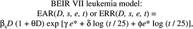
(12-3)
where D is dose (Sv), s is sex, and e* is (e − 30) / 10 for e < 30 and 0 for e 30 ( e is age at exposure in years). Table 12-3 shows the parameter estimates, and Figure 12-2 depicts the dependence of the ERR or EAR on age at exposure and time since exposure. The parameter θ indicates the degree of curvature, which does not depend on sex, age at exposure, or time since exposure; βM and βF represent the ERR/Sv or the EAR (expressed as excess deaths per 104 PY-Sv, where PY = person-years), for exposure at age 30 or more at 25 years following exposure. This model was found to fit the data better than analogous models using e instead of e*, or using t instead of log (t), and nearly as well as models with a
TABLE 12-3 Committee’s Preferred ERR and EAR Models for Estimating Leukemia Incidence and Mortalitya,b,c
|
Parameter |
ERR Model |
EAR Model |
|
βM |
1.1 per Sv (0.1, 2.6) |
1.62 deaths per 104 PY-Sv (0.1, 3.6) |
|
βF |
1.2 per Sv (0.1, 2.9) |
0.93 deaths per 104 PY-Sv (0.1, 2.0) |
|
γ |
−0.40 per decade (−0.78, 0.0) |
0.29 per decade (0.0, 0.62) |
|
δ |
−0.48 (−1.1, 0.2) |
0.0 |
|
|
0.42 (0.0, 0.96) |
0.56 (0.31, 0.85) |
|
θ |
0.87 per Sv (0.16, 15) |
0.88 Sv−1 (0.16, 15) |
|
NOTE: Estimated parameters with 95% CIsd based on likelihood ratio profile. aThe ERR or EAR is of the form βs(D + θ D2) exp [γ e* + δ log (t / 25) + bBased on analyses of LSS mortality data (1950–2000), with 296 deaths from leukemia. cThese models apply only to the period 5 or more years following exposure. dConfidence intervals based on likelihood ratio profile. |
||
categorical treatment of age at exposure. It was also found to be necessary to allow the dependence on time since exposure to vary by age at exposure by including the term e* log (t / 25). For the EAR model, there was no need to include a term for the main effect of time since exposure; note that with this parameterization, there is no decrease with time since exposure for those exposed at age 30 or more. For application of these models, the reader should consult the section “Use of the Committee’s Preferred Models to Estimate Risks for the U.S. Population.”
USE OF THE COMMITTEE’S PREFERRED MODELS TO ESTIMATE RISKS FOR THE U.S. POPULATION
To use models developed primarily from Japanese A-bomb survivor data for the estimation of lifetime risks for the U.S. population, several issues must be addressed. These include determining approaches for estimating risks at low doses and low dose rates, projecting risks over time, transporting risks from the Japanese to the U.S. population, and estimating risks from exposure to X-rays. This section describes the approach for addressing each of these issues, as well as the methodology used to estimate lifetime risk. More detailed discussion of some of the issues is given in Chapter 10, and the approach for quantifying the uncertainties associated with some of these issues is discussed later in this chapter.
Estimating Risks from Exposure to Low Doses and Low Dose Rates
The BEIR VII risk models have been developed primarily from analyses of data on the LSS cohort of Japanese A-bomb survivors. Although more than 60% of the exposed members of this cohort were exposed to relatively low doses (0.005–0.1 Sv), survivors who were exposed to doses exceeding 0.5 Gy are still influential in estimating the ERR/Sv. In addition, exposure of A-bomb survivors was at high dose rates, whereas exposure at low dose rates is of primary concern for risk assessment. Based on evidence from experimental data, ICRP (1991), NCRP (1993), EPA (1999), and UNSCEAR (2000b) recommended reducing linear estimates based on A-bomb survivor (or other high-dose-rate) exposure by a dose and dose-rate reduction factor (DDREF) of 2.0.
In Chapter 10, both data on solid cancer risks in the LSS cohort and experimental data pertinent to this issue are evaluated by the committee. Based on this evaluation, the committee found a believable range of DDREF values (for adjusting linear risk estimates based on the LSS cohort) to be 1.1 to 2.3. When a single value is needed, 1.5 (the median of the subjective probability distribution for the LSS DDREF) is used to estimate risk for solid tumors. To estimate the risk of leukemia, the BEIR VII model is linear-quadratic, since this model fitted the data substantially better than the linear model.
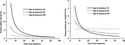
FIGURE 12-2 Age-time patterns in radiation-associated risks for leukemia mortality. Curves are sex-averaged estimates of the risk at 1 Sv for people exposed at age 10 (solid lines), age 20 (dashed lines), and age 30 or more (dotted lines). Estimates were computed using the parameter estimates shown in Table 12-3.
Projection of Risks over Time
The LSS cohort has now been followed for more than 50 years, so that lifetime follow-up is nearly complete for all but the youngest survivors (under age 20 at exposure). Although the extrapolation involved in estimating lifetime risks based on limited follow-up has been a major source of uncertainty in past risk assessments, it is now much less so. The BEIR VII models allow for dependencies of both the ERR and the EAR on attained age, and it is assumed that the identified patterns persist until the end of life for the youngest survivors. Additional discussion of this issue is found in Chapter 10.
For leukemia, the early years of follow-up also must be addressed. Ascertainment of leukemia cases for the LSS cohort did not begin until 1950, while data on medically exposed cohorts have demonstrated that excess leukemia cases can occur as early as a year or two after exposure (Boice and others 1987; Curtis and others 1992, 1994; Inskip and others 1993; Weiss and others 1994, 1995). In several of these studies, relative risks were highest in the period 1–5 years after exposure. In addition, a recent analysis of data on Mayak workers found that leukemia risks 3–5 years following external radiation exposure were more than an order of magnitude higher than risks for later periods (Shilnikova and others 2003). The UNSCEAR (2000b) committee addressed this problem by assuming that excess risks for the first 5 years after exposure were half those observed 5 years after exposure. The BEIR VII committee has instead assumed that excess absolute risk in the period 2–5 years following exposure is equal to that observed 5 years after exposure. Clearly there is uncertainty in the magnitude of the risk during the initial years following exposure.
Transport of Risks from a Japanese to a U.S. Population
Baseline risks for many site-specific cancers are different for the United States and Japan. For example, baseline risks for cancers of the colon, lung, and female breast are higher in the United States, whereas baseline risks for cancers of the stomach and liver are much higher in Japan. The BEIR V committee based its estimates on relative risk transport, where it is assumed that the excess risk due to radiation is proportional to baseline risks; that is, the ERR is the same for the United States and Japan. However, the BEIR III committee based its estimates on absolute risk transport, where it is assumed that the excess risk does not depend on baseline risks; that is, the EAR is the same for the United States and Japan. The EPA (1994) used the geometric mean of the two estimates, whereas UNSCEAR (2000b) presented estimates based on both approaches without indicating a preference. Estimates based on relative and absolute risk can differ substantially. For example, the UNSCEAR stomach cancer estimates for the U.S. population based on absolute risk transport are nearly an order of magnitude larger than those based on relative risk transport.
For breast and thyroid cancer, the committee’s models are based on combined analyses that include Caucasian subjects. For other solid cancer sites including leukemia, the committee has calculated risks using both relative and absolute risk transport, which provides an indication of the uncertainty from this source. The recommended point estimates are weighted means of estimates obtained under the two models (adjusted by a DDREF of 1.5 as discussed above). For sites other than breast, thyroid, and lung, a weight of 0.7 is used for the estimate obtained using relative risk transport and a weight of 0.3 for the estimate obtained using absolute
risk transport, with the weighting done on a logarithmic scale. This choice was made because, as discussed in Chapter 10, there is somewhat greater support for relative risk than for absolute risk transport. In addition, the ERR models used to obtain relative risk transport estimates may be less vulnerable to possible bias from underascertainment of cases. For lung cancer, the weighting scheme is reversed, and a weight of 0.7 is used for the absolute risk transport estimate and a weight of 0.3 for the relative risk transport estimate. This departure was made because of evidence that the interaction of radiation and smoking in A-bomb survivors is additive (Pierce and others 2003). Although it is likely that the correct transport model varies by cancer site, for sites other than breast, thyroid, and lung the committee judged that current knowledge was insufficient to allow the approach to vary by cancer site.
Transport has not generally been considered an important source of uncertainty for estimating leukemia risks. The committee has nevertheless developed both ERR and EAR models for leukemia and obtained estimates based on both relative and absolute risk transport. As shown later, the EAR model leads to substantially lower lifetime risks than the ERR model (Table 12-7). Since there is no reason to suspect underascertainment of leukemia deaths, apparently this comes about because baseline risks in the LSS cohort are different than those for a modern U.S. population. Because of the small number of deaths in the early period among those who were unexposed, it might be thought that the uncertainty in the estimated ERR/Sv would be large; however in fact, it is only slightly larger than that for the EAR model (Table 12-3).
Relative Effectiveness of X-Rays and γ-Rays
Risk estimates in this report have been developed primarily from data on A-bomb survivors and are thus directly relevant to exposure from high-energy photons. However, the report is concerned with low-LET radiation generally, which includes γ-rays, X-rays, and fast electrons. There is no principal difference between the action of these different types of radiation, because they all work through fast electrons that either are incident on the body or are released within the body by electrons or photons. The various types of low-LET radiation vary in their ability to penetrate to greater depths in the body. The more penetrating, high-energy radiation tends to produce electrons with linear energy transfer less than 1 keV / μm, while the softer X-rays release slower electrons with linear energy transfer up to several kiloelectronvolts per micrometer.
With regard to setting dose limits in radiation protection, γ-rays, fast electrons, and X-rays are all given the radiation weighting factor 1; that is, an absorbed dose of 1 Gy of these radiations is taken to be equal to the effective dose 1 Sv (ICRP 1991), which expresses the fact that the differences of effectiveness between different photon radiations are not considered of sufficient consequence to require explicit accounting in radiation protection regulations. However, the significant difference between the (dose average) unrestricted LET of 60Co (about 0.4keV / μm) or 137Cs γ-rays (about 0.8keV / μm) and that of 200 kVp X-rays (about 3.5keV / μm) makes it clear that the relative biological effectiveness (RBE) at low doses can differ appreciably for γ-rays and X-rays. For actual risk estimates it is, therefore, necessary to consider these differences in terms of the radiobiological findings, the dosimetric and microdosimetric parameters of radiation quality, and the radioepidemiologic evidence.
As discussed in ICRP (2004) and in Chapters 1 and 3 of this report, there is evidence based on chromosomal aberration data and on biophysical considerations that, at low doses, the effectiveness per unit absorbed dose of standard X-rays may be about twice that of high-energy photons. The effectiveness of lower-energy X-rays may be even higher. How this translates into risks of late effects in man is an open question. Estimates based on studies of persons exposed to X-rays for medical reasons tend to be lower than those based on A-bomb survivors (Little 2001; ICRP 2004), but a number of other differences may confound these comparisons. In addition, doses in many medically exposed populations are higher than those at which the energy of the radiation (based on biophysical considerations) would be expected to be important.
Because of the lack of adequate epidemiologic data on this issue, the committee makes no specific recommendation for applying risk estimates in this report to estimate risk from exposure to X-rays. However, it may be desirable to increase risk estimates in this report by a factor of 2 or 3 for the purpose of estimating risks from low-dose X-ray exposure.
Relative Effectiveness of Internal Exposure
Internal exposure through inhalation or ingestion is also of interest. For example, internal exposure to 131I, strontium, and cesium may occur from atmospheric fallout from nuclear weapons testing. Epidemiologic studies involving these exposures are reviewed in Chapter 9. Studies of thyroid cancer in relation to 131I include those of persons exposed to atmospheric fallout in Utah, to releases from the Hanford plant, and as a result of the Chernobyl accident. There are also studies of persons exposed to cesium and strontium from releases from the Mayak nuclear facility in Russia into the Techa River. To date, these studies are not adequate to quantify carcinogenic risk reliably as a function of dose. Although there are no strong reasons to think that the dose-response from internal low-LET exposure would differ from that for external exposure, there is additional uncertainty in applying the BEIR VII risk models to estimate risks from internal exposure.
Method of Calculating Lifetime Risks
Several measures of lifetime risk have been used to express radiation risks and are discussed by Vaeth and Pierce (1990), Thomas and colleagues (1992), UNSCEAR (2000b), and Kellerer and colleagues (2001). The BEIR VII committee has chosen to use what Kellerer and coworkers refer to as the lifetime attributable risk (LAR), which was earlier called the risk of untimely death by Vaeth and Pierce (1990). The LAR is an approximation of the risk of exposure-induced death (REID), the measure used by UNSCEAR (2000b), which estimates the probability that an individual will die from (or develop) cancer associated with the exposure. Although the nomenclature is recent, the LAR was used by the BEIR III committee (1980b) and by the EPA (1994).
The LAR and the REID both differ from the excess lifetime risk (ELR) used by the BEIR V committee in that the former include deaths or incident cases of cancer that would have occurred without exposure but occurred at a younger age because of the exposure. As noted by Thomas and colleagues (1992) and earlier by Pierce and Vaeth (1989), the ratio of ELR to REID is approximately 1 − Qc where Qc is the lifetime risk of dying from the cause of interest. For example, the ELR for all cancer mortality would be about 20% lower than the REID. The LAR differs from the REID in that the survival function used in calculating the LAR does not take account of persons dying of radiation-induced disease, thus simplifying the computations. This difference may be important for estimating risks at higher doses (1+ Sv), but not at the low doses of interest for this report. Kellerer and colleagues show that the REID and the LAR are nearly identical at low doses and discuss other aspects of the LAR compared to the REID.
The LAR for a person exposed to dose D at age e is calculated as follows:
(12-4)
where the summation is from a = e + L to l00, where a denotes attained age (years) and L is a risk-free latent period (L = 5 for solid cancers; L = 2 for leukemia). The M(D, e, a) is the EAR, S(a) is the probability of surviving until age a, and S(a)/S(e) is the probability of surviving to age a conditional on survival to age e. All calculations are sex-specific; thus, the dependence of all quantities on sex is suppressed.
The quantities S(a) were obtained from a 1999 unabridged life table for the U.S. population (Anderson and DeTurk 2002). Lifetime risk estimates using relative risk transport were based on ERR models. For these calculations,
for cancer incidence, and
for cancer mortality. The ERR(D, e, a) was obtained from models shown in Tables 12-1, 12-2, and 12-3. The λIc(a) represents sex- and age-specific 1995–1999 U.S. cancer incidence rates from Surveillance Epidemiology, and End Results (SEER) registries, whereas the λMc (a) are sex- and age-specific 1995–1999 U.S. cancer mortality rates (http://seer.cancer.gov/csr/1975_2000), where c designates the cancer site or category. These rates were available for each 5-year age group with linear interpolation used to develop estimates for single years of age. With the exception of the category “all solid cancers,” the same ERR models were used to estimate both cancer incidence and mortality.
Lifetime risk estimates using absolute risk transport were based on EAR models (see “Transport of Risks from a Japanese to a U.S. Population”). For estimating cancer incidence, M(D, e, a) is taken to be the EAR(D, e, a) based on the models shown in Tables 12-1, 12-2, and 12-3. For estimating mortality from all solid cancers, the EAR mortality model shown in Table 12-1 was used directly. For estimating site-specific cancer mortality, it was necessary to adjust the EAR(D, e, a) from Tables 12-2 and 12-3 by multiplying by λMc (a)/λIc (a), the ratio of the sex- and age-specific mortality and incidence rates for the U.S. population. That is, for site-specific mortality,
Leukemia merits special comment. The approach for deriving incidence and mortality estimates based on relative and absolute risk transport is the same for leukemia as for other site-specific cancers, despite the fact that leukemia models were developed from LSS mortality data rather than incidence data as for other sites. This is because LSS leukemia data were obtained at a time when this disease was nearly always rapidly fatal, so that estimates of leukemia mortality should closely approximate those for leukemia incidence. In the last few decades, however, marked progress has been made in treating leukemia, and the disease is not always fatal. Thus, the committee has used the EAR model shown in Table 12-3 to estimate leukemia incidence, but has adjusted the EAR(D, s, e, a) from Table 12-3 in the manner described above to obtain estimates of leukemia mortality. In all cases, the U.S. leukemia baseline rates were for all leukemias excluding CLL.
Models for leukemia differ from those for solid cancers in that risk is expressed as a function of age at exposure (e) and time since exposure (t) instead of age at exposure and attained age (a). Since t = a − e, ERR(D, e, a) or EAR(D, e, a) is obtained by substituting a − e for t in the models presented in Table 12-3. Note further that for the period 2–5 years after exposure, the EAR is assumed to be the same as that at 5 years after exposure. That is, for a = e + 2 to e + 5, M(D, e, a) = M(D, e, e + 5).
The approach described above for obtaining estimates based on absolute transport differs from that used by UNSCEAR (2000b) and NIH (2003), where M(D, e, a) for
absolute risk transport was calculated by multiplying the ERR(D, e, a) estimated from LSS data by sex- and age-specific baseline risks for the 1985 population of Japan. Because Japanese rates for cancer of several sites changed in the period 1950–1985 (becoming more similar to U.S. rates), the committee’s approach may reflect risks more truly in the LSS cohort than do 1985 baseline rates for Japan.
Another difference between the committee’s approach and that of UNSCEAR is that for estimating cancer incidence, UNSCEAR lifetime risk calculations counted only first cancers. That is, once a person was diagnosed with cancer (baseline or radiation induced), that person was removed from the population at risk. By contrast, the committee’s calculations count all primary cancers including those in persons previously diagnosed with another primary cancer.
To obtain estimates of risk for a population of mixed exposure ages, the age-at-exposure-specific estimates in Equation (12-4) were weighted by the fraction of the population in the age group based on the U.S. population in 1999 (http://wonder.cdc.gov/popu0.shtml). Estimates of chronic lifetime exposure are for a person at birth, with allowance for attrition of the population with age. These estimates are obtained by weighting the age-at-exposure-specific estimates by the probability of survival to each age, that is, S(e). Similarly, estimates for chronic occupational exposure are for a person who enters the workforce at age 18 and continues to be exposed to age 65, again with allowance for attrition of the population with age. These estimates are obtained by weighting the age-at-exposure-specific estimates by the probability of survival to each age conditional on survival to age 18, that is, S(e)/S(18).
QUANTITATIVE EVALUATION OF UNCERTAINTY IN LIFETIME RISKS
Because of the various sources of uncertainty it is important to regard specific estimates of LAR with a healthy skepticism, placing more faith in a range of possible values. Although a confidence interval is the usual statistical device for doing so, the approach here also accounts for uncertainties external to the data, treating subjective probability distributions for these uncertainties as if they resulted from real data. The resulting range of plausible values for lifetime risk is consequently labeled a “subjective confidence interval” to emphasize its dependence on opinions in addition to direct numerical observation. Similar logic has been used in other uncertainty analyses (NCRP 1997; EPA 1999; UNSCEAR 2000b).
The quantitative analysis focuses on the three sources that are thought to matter most: (1) sampling variability in risk model parameter estimates from the LSS data, (2) the uncertainty about transport of risk from a Japanese (LSS) to a U.S. population (i.e., whether ERR or EAR is transportable), and (3) the uncertainty in the appropriate value of a DDREF for adjusting low-dose risks based on linear-in-dose risk models estimated from LSS data. The approach used is a conventional one that finds a variance for the estimated LAR (on the log scale) induced by the variances of these three sources. The computational approach for the subjective confidence intervals is detailed in Annex 12C. Additional sources of uncertainty that have not been quantified are discussed later in the chapter. For site-specific cancers other than leukemia, the assessment of sampling variability did not include uncertainty in the parameters quantifying the modifying effects of age at exposure and attained age. Although estimates of solid cancer risks are obtained as the sum of site-specific risks, the uncertainty in these estimates was evaluated using models for all solid cancers.
RESULTS OF RISK CALCULATIONS
Lifetime Risk Estimates for the U.S. Population
In this section, the committee’s preferred estimates of the LAR are presented for several cancer categories. Estimates of the numbers of excess cancers or deaths due to cancer in a population of 100,000 exposed to 0.1 Gy are emphasized and are intended to apply to a population with an age composition similar to the 1999 U.S. population. In addition, estimates for all solid cancers and for leukemia are presented for three specific exposure ages (10, 30, and 50 years), for a population that is exposed throughout life to 1 mGy per year, and for a population that is exposed to 10 mGy per year from age 18 to 65. Additional examples are found in Annex 12D.
For perspective, Table 12-4 shows lifetime risks of cancer incidence and mortality in the absence of exposure. For
TABLE 12-4 Baseline Lifetime Risk Estimates of Cancer Incidence and Mortality
|
Cancer site |
Incidence |
Mortality |
||
|
Males |
Females |
Males |
Females |
|
|
Solid cancera |
45,500 |
36,900 |
22,100 (11) |
17,500 (11) |
|
Stomach |
1,200 |
720 |
670 (11) |
430 (12) |
|
Colon |
4,200 |
4,200 |
2,200 (11) |
2,100 (11) |
|
Liver |
640 |
280 |
490 (13) |
260 (12) |
|
Lung |
7,700 |
5,400 |
7,700 (12) |
4,600 (14) |
|
Breast |
— |
12,000 |
— |
3,000 (15) |
|
Prostate |
15,900 |
— |
3,500 (8) |
— |
|
Uterus |
— |
3,000 |
— |
750 (15) |
|
Ovary |
— |
1,500 |
— |
980 (14) |
|
Bladder |
3,400 |
1,100 |
770 (9) |
330 (10) |
|
Other solid cancer |
12,500 |
8,800 |
6,800 (13) |
5,100 (13) |
|
Thyroid |
230 |
550 |
40 (12) |
60 (12) |
|
Leukemia |
830 |
590 |
710 (12) |
530 (13) |
|
NOTE: Number of estimated cancer cases or deaths in population of 100,000 (No. of years of life lost per death). aSolid cancer incidence estimates exclude thyroid and nonmelanoma skin cancers. |
||||
nearly all sites other than breast, ovary, and thyroid, risks are higher for males than females, with especially large differences for cancers of the liver and bladder. In males, prostate cancer accounts for more than a third of the incident cases. In females, breast cancer accounts for about a third of the incident cases.
Tables 12-5A and 12-5B show estimates of the LAR for a population with an age composition similar to that of the U.S. population exposed to 0.1 Gy. Estimates of cancer incidence (Table 12-5A) and mortality (Table 12-5B) are shown for several site-specific solid cancers. The committee’s preferred estimates are those in the third and sixth columns. These were obtained by calculating a weighted mean (on a logarithmic scale) of linear estimates based on relative and absolute risk transport (also shown) and then reducing them by DDREF of 1.5 as described earlier. The subjective confidence intervals reflect uncertainty due to sampling variability, transport, and DDREF. For most sites, these intervals cover at least an order of magnitude. For many sites, statistical uncertainty alone is large (see Table 12-2). For cancers of the stomach, liver, lung (females), prostate, and uterus, estimates based on relative and absolute risk differ by a factor of 2 or more, contributing substantially to the uncertainty in estimates for these sites. It is perhaps surprising that the LAR for lung cancer is nearly twice as high for females as males even though the baseline risks show a reverse pattern. It is possible that this and other patterns for site-specific cancers reflect statistical anomalies or other biases in LARs estimated with high uncertainty.
The committee’s preferred estimates for risk of all solid cancers can be obtained as the sums of the site-specific estimates and are shown in the next-to-the-last line of Tables 12-5A and 12-5B. These estimates are higher for females than males, even though the reverse is true for baseline risks (Table 12-4), a finding that comes about primarily because of the contribution of breast cancer and lung cancer (as noted above). For cancer mortality, the years of life lost per death are also of interest. For the sum of sites estimates, this was 14 per death for males and 15 per death for females.
The LAR for all cancer incidence is about twice that for cancer mortality. However, this ratio varies greatly by cancer site. The largest contribution to cancer incidence in males is from the residual category of “other solid cancers” followed by colon and lung cancer. These three categories are also the most important contributors to cancer mortality. Cancers of the lung, and breast and other solid cancers con-
TABLE 12-5A Lifetime Attributable Risk of Solid Cancer Incidence
|
Cancer Site |
Males |
Females |
||||
|
LAR Based on Relative Risk Transporta |
LAR Based on Absolute Risk Transportb |
LAR Based on Relative Risk Transporta |
LAR Based on Absolute Risk Transportb |
|||
|
Incidence |
||||||
|
Stomach |
25 |
280 |
34 (3, 350) |
32 |
330 |
43 (5, 390) |
|
Colon |
260 |
180 |
160 (66, 360) |
160 |
110 |
96 (34, 270) |
|
Liver |
23 |
150 |
27 (4, 180) |
9 |
85 |
12 (1, 130) |
|
Lung |
250 |
190 |
140 (50, 380) |
740 |
370 |
300 (120, 780) |
|
Breast |
|
510 Not used |
460 |
310 (160, 610) |
||
|
Prostate |
190 |
6 |
44 (<0, 1860) |
|
||
|
Uterus |
|
19 |
81 |
20 (<0, 131) |
||
|
Ovary |
66 |
47 |
40 (9, 170) |
|||
|
Bladder |
160 |
120 |
98 (29, 330) |
160 |
100 |
94 (30, 290) |
|
Other |
470 |
350 |
290 (120, 680) |
490 |
320 |
290 (120, 680) |
|
Thyroid |
32 |
No model |
21 (5, 90) |
160 |
No model |
100 (25, 440) |
|
Sum of site-specific estimates |
1400 |
1310e |
800 |
2310f |
2060e |
1310 |
|
All solid cancer modelg |
1550 |
1250 |
970 (490, 1920) |
2230 |
1880 |
1410 (740, 2690) |
|
NOTE: Number of cases per 100,000 persons of mixed ages exposed to 0.1 Gy. aLinear estimate based on ERR models shown in Table 12-2 with no DDREF adjustment. bLinear estimate based on EAR models shown in Table 12-2 with no DDREF adjustment. cEstimates obtained as a weighted average (on a logarithmic scale) of estimates based on relative and absolute risk transport. For sites other than lung, breast, and thyroid, relative risk transport was given a weight of 0.7 and absolute risk transport was given a weight of 0.3. These weights were reversed for lung cancer. Models for breast and thyroid cancer were based on data that included Caucasian subjects. The resulting estimates were reduced by a DDREF of 1.5. dIncluding uncertainty from sampling variability, transport, and DDREF. Sampling uncertainty in the parameters that quantify the modifying effects of age at exposure and attained age is not included except for the all solid cancer model. eIncludes thyroid cancer estimate based on ERR model. fIncludes breast cancer estimate based on EAR model. gEstimates based on model developed by analyzing LSS incidence data on all solid cancers excluding thyroid cancer and nonmelanoma skin cancer as a single category. See Table 12-1. |
||||||
TABLE 12-5B Lifetime Attributable Risk of Solid Cancer Mortality
|
Cancer Site |
Males |
Females |
||||
|
LAR Based on Relative Risk Transporta |
LAR Based on Absolute Risk Transportb |
LAR Based on Relative Risk Transporta |
LAR Based on Absolute Risk Transportb |
|||
|
Stomach |
14 |
150 |
19 (2, 190) |
19 |
190 |
25 (3, 220) |
|
Colon |
130 |
89 |
76 (32, 180) |
78 |
50 |
46 (16, 130) |
|
Liver |
16 |
120 |
20 (3, 150) |
8 |
84 |
11 (1, 130) |
|
Lung |
240 |
200 |
140 (52, 380) |
620 |
340 |
270 (110, 660) |
|
Breast |
|
110 Not used |
110 |
73 (37, 150) |
||
|
Prostate |
35 |
1 |
9 (<0, 300) |
|
||
|
Uterus |
|
4 |
24 |
5 (<0, 38) |
||
|
Ovary |
37 |
34 |
24 (6, 98) |
|||
|
Bladder |
34 |
31 |
22 (7, 73) |
45 |
36 |
28 (10, 81) |
|
Other |
180 |
190 |
120 (54, 280) |
200 |
180 |
132 (61, 280) |
|
Sum of site-specific estimates |
650 |
780 |
410 |
1120e |
1050 |
610 |
|
All solid cancer modelf |
760 |
650 |
480 (240, 980) |
1200 |
940 |
740 (370, 1500) |
|
NOTE: Number of deaths per 100,000 exposed persons of mixed ages exposed to 0.1 Gy. aLinear estimate based on ERR models shown in Table 12-2 with no DDREF adjustment. bLinear estimate based on EAR models shown in Table 12-2 with no DDREF adjustment. cEstimates obtained as a weighted average (on a logarithmic scale) of estimates based on relative and absolute risk transport. For sites other than lung, breast, and thyroid, relative risk transport was given a weight of 0.7 and absolute risk transport was given a weight of 0.3. These weights were reversed for lung cancer. Models for breast and thyroid cancer were based on data that included Caucasian subjects. The resulting estimates were reduced by a DDREF of 1.5. dIncluding uncertainty from sampling variability, transport, and DDREF. Sampling uncertainty in the parameters that quantify the modifying effects of age at exposure and attained age is not included except for the all solid cancer model. eIncludes breast cancer estimate based on EAR model. fEstimates based on model developed by analyzing LSS mortality data on all solid cancers as a single category. See Table 12-1. |
||||||
tribute about equally to cancer incidence in females. Lung cancer is the most important contributor to cancer mortality in females.
Although the committee’s preferred estimates for all solid cancers are the sums of the site-specific estimates, for comparison the last line of Tables 12-5 shows estimates based on models developed by analyzing LSS data incidence and mortality data on all solid cancers as a single category (see Table 12-1). These estimates are generally about 20% higher than those obtained using the sum-of-sites approach, a difference that comes about in part because of the weighting scheme used to combine estimates based on relative and absolute risk transport (particularly the greater weight given to absolute risk transport for lung cancer) and because of the use of the model developed by Preston and colleagues (2002a) for breast cancer, similar to assuming absolute risk transport for this site.
Table 12-6 shows estimates of the all solid cancer LARs for several exposure scenarios. In each case, these were obtained as the sum of the site-specific estimates. Additional detail is given in Annex 12D. Because models for most cancers allow for a decrease in both the ERR and the EAR with increasing age at exposure, estimates for persons exposed at age 10 are more than twice those for persons exposed at ages 30 or 50. However, because models allow for no further decrease after age 30, the difference in lifetime risk estimates for persons exposed at ages 30 and 50 is not as great. Also shown are estimates of the LAR for chronic lifetime exposure to 1 mGy per year and of the LAR for an occupational scenario of exposure to 10 mGy per year from ages 18 to 65.
Table 12-7 shows estimates of the LARs for leukemia incidence and mortality for several exposure scenarios. The number of years of life lost per death was estimated to be 20 years for males and 21 years for females, values that are greater than those for solid cancers. Although the transport model has not been considered a major source of uncertainty in leukemia risk estimates (UNSCEAR 2000b; NIH 2003), Table 12-7 shows that LAR estimates based on relative risk transport are higher than those based on absolute risk transport, with the ratio ranging from about 1 to 3. This is not due to the contribution of CLL since that was excluded from the baseline rates used to calculate LARs based on relative risk transport. The committee’s preferred estimates are based on a weighted mean of LAR estimates obtained from the two transport models as with most site-specific solid cancers, and the subjective confidence intervals include transport uncertainty. Unlike solid cancer models, the leukemia models (Table 12-3) are based on linear-quadratic functions of dose, so there is no need for further reduction by a DDREF. Uncertainty calculations include sampling uncertainty in both the linear coefficient and the curvature parameter. Previous risk assessments have considered leukemia incidence and
TABLE 12-6 Committee’s Preferred Estimates of Lifetime Attributable Risk (LAR) of Solid Cancer Incidence and Mortalitya (with 95% subjective CIs)b
|
Exposure Scenario |
Incidence |
Mortality |
||
|
Males |
Females |
Males |
Females |
|
|
0.1 Gy to population of mixed ages |
800 (400, 1590) |
1310 (690, 2490) |
410 (200, 830) |
610 (300, 1230) |
|
0.1 Gy at age 10 |
1330 (660, 2660) |
2530 (1290, 4930) |
640 (300, 1390) |
1050 (470, 2330) |
|
0.1 Gy at age 30 |
600 (290, 1260) |
1000 (500, 2020) |
320 (150, 650) |
490 (250, 950) |
|
0.1 Gy at age 50 |
510 (240, 1100) |
680 (350, 1320) |
290 (140, 600) |
420 (210, 810) |
|
1 mGy per year throughout life |
550 (280, 1100) |
970 (510, 1840) |
290 (140, 580) |
460 (230, 920) |
|
10 mGy per year from ages 18 to 65 |
2600 (1250, 5410) |
4030 (2070, 7840) |
1410 (700, 2860) |
2170 (1130, 4200) |
|
NOTE: Number of cases or deaths per 100,000 exposed persons. aThese were obtained as the sum of site-specific LAR estimates. The site-specific estimates were obtained as a weighted average (on a logarithmic scale) of estimates based on relative and absolute risk transport. For sites other than lung, breast, and thyroid, relative risk transport was given a weight of 0.7 and absolute risk transport was given a weight of 0.3. These weights were reversed for lung cancer. Models for breast and thyroid cancer were based on data that included Caucasian subjects. The resulting linear estimates were reduced by a DDREF of 1.5. bIncluding uncertainty from sampling variability, transport, and DDREF. The uncertainty evaluation was based on evaluation of estimates based on analyses of LSS cohort data on all solid cancers analyzed as a single category as described in Annex 12C. |
||||
TABLE 12-7 Lifetime Attributable Risk of Leukemia Incidence and Mortalitya
|
Exposure Scenario |
Males |
Females |
||||
|
LAR Based on Relative Risk Transportb |
LAR Based on Absolute Risk Transportc |
LAR Based on Relative Risk Transportb |
LAR Based on Absolute Risk Transportc |
|||
|
Incidence |
||||||
|
0.1 Gy to population of mixed ages |
120 |
64 |
100 (33, 300) |
94 |
38 |
72 (21, 250) |
|
0.1 Gy at age 10 |
140 |
85 |
120 (40, 360) |
110 |
50 |
86 (25, 300) |
|
0.1 Gy at age 30 |
87 |
77 |
84 (31, 230) |
69 |
49 |
62 (22, 170) |
|
0.1 Gy at age 50 |
110 |
45 |
84 (24, 290) |
84 |
30 |
62 (16, 230) |
|
1 mGy per year throughout life |
83 |
40 |
67 (19, 230) |
68 |
26 |
51 (13, 200) |
|
10 mGy per year from ages 18 to 65 |
430 |
240 |
360 (110, 1140) |
340 |
160 |
270 (79, 920) |
|
Mortality |
||||||
|
0.1 Gy to population of mixed ages |
88 |
40 |
69 (22, 220) |
71 |
25 |
52 (14, 190) |
|
0.1 Gy at age 10 |
88 |
42 |
70 (21, 240) |
71 |
26 |
53 (13, 210) |
|
0.1 Gy at age 30 |
70 |
53 |
64 (23, 180) |
59 |
36 |
51 (17, 150) |
|
0.1 Gy at age 50 |
93 |
37 |
71 (20, 250) |
74 |
26 |
54 (14, 210) |
|
1 mGy per year throughout life |
62 |
25 |
47 (13, 180) |
53 |
17 |
38 (9, 160) |
|
10 mGy per year from ages 18 to 65 |
350 |
170 |
290 (84, 970) |
290 |
120 |
220 (61, 820) |
|
NOTE: Number of cases or deaths per 100,000 exposed persons. aAll estimates are based on linear-quadratic model. bBased on ERR model shown in Table 12-4. cBased on EAR model shown in Table 12-4. dObtained as a weighted mean (on a logarithmic scale) with weights of 0.7 for the relative risk transport estimate and a weight of 0.3 for the absolute risk transport estimate. eIncluding uncertainty from sampling variability and transport. Sampling uncertainty includes uncertainty in both the linear and the quadratic terms of the dose-response. |
||||||
mortality to be very similar, and this was likely the case at the time many of the LSS leukemia data were obtained. However, currently leukemia is not always rapidly fatal, and the committee has thus reduced estimates based on the LSS cohort for estimating leukemia mortality (see “Methods of Calculating Lifetime Risks”). For a single exposure of a population of mixed ages to 0.1 Gy, leukemia mortality estimates are about 30% lower than those for leukemia incidence.
Detailed tables showing lifetime risk estimates are found in Annex 12D. Annex 12D also gives examples of the use of these tables to obtain risk estimates for specific exposure scenarios.
Comparison of BEIR VII Risk Estimates with Those from Other Sources
Tables 12-8 and 12-9 compare the BEIR VII committee’s lifetime risk estimates with estimates recommended by other organizations in recent years. A description of the ap
TABLE 12-8 Comparison of BEIR VII Lifetime Cancer Mortality Estimates with Those from Other Reports
|
Cancer Category |
BEIR Va (NRC 1990) |
ICRPb (1991) |
EPAb (1999) |
UNSCEARc (2000) |
BEIR VIId |
|
|
Leukemiae |
95 50 |
56 |
50 |
|
|
61 |
|
All cancer except leukemia (sum) |
700 (460) |
450 |
520 |
|
||
|
All solid cancers (sum) |
|
510 |
||||
|
Digestive cancers |
230 (150) |
|
||||
|
Esophagus |
|
30 |
12 |
30, 60 |
(25) |
|
|
Stomach |
110 |
41 |
15, 120 |
(18) |
22 |
|
|
Colon |
85 |
100 |
160, 50 |
(75) |
61 |
|
|
Liver |
15 |
15 |
20, 85 |
(20) |
16 |
|
|
Respiratory cancer |
170 (110) |
|
||||
|
Lung |
|
85 |
99 |
340, 210 |
(160) |
210 |
|
Female breastg |
35 (23) |
20 |
51 |
280, 65 |
(43) |
37 |
|
Bone |
|
5 |
1 |
— |
|
|
|
Skin |
|
2 |
1 |
— |
|
|
|
Prostateg |
|
5 |
||||
|
Uterusg |
3 |
|||||
|
Ovaryg |
|
10 |
15 |
|
|
12 |
|
Bladder |
30 |
24 |
40, 20 |
(22) |
25 |
|
|
Kidney |
— |
5 |
— |
|
||
|
Thyroid |
8 |
3 |
— |
|||
|
Other cancers or other solid cancersh |
260 (170) |
50 |
150 |
280, 180 |
(160) |
130 |
|
NOTE: Excess deaths for population of 100,000 of all ages and both sexes exposed to 0.1 Gy. aAverage of estimates for males and females. The measure used was the excess lifetime risk; unlike other estimates in this table, radiation-induced deaths in persons who would have died from the same cause at a later time in the absence of radiation exposure are excluded. The estimates are not reduced by a DDREF, but parentheses show the result that would be obtained if the DDREF of 1.5, used by the BEIR VII committee, had been employed. bExcept for the EPA breast and thyroid cancer estimates, the solid cancer estimates are linear estimates reduced by a DDREF of 2. cAverage of estimates for males and females. Except where noted otherwise, estimates are based on the attained-age model. The first estimate is based on relative risk transport; the second on absolute risk transport. The estimate in parentheses is a combined estimate (using the same weights as used by the BEIR VII committee applied on a logarithmic scale) reduced by a DDREF of 1.5, although these were not recommendations of the UNSCEAR committee. dAverage of the committee’s preferred estimates for males and females from Table 12-5B. eEstimates based on a linear-quadratic model. fEstimates based on age-at-exposure model. gThese estimates are half those for females only. hThese estimates are for the remaining solid cancers. |
||||||
proaches used to obtain these earlier risk estimates is given in Annex 12A. The ICRP and EPA solid cancer estimates include reduction by a DDREF of 2 (except for the EPA estimates for breast and thyroid cancers, where linear estimates were used without reduction). Neither BEIR V nor UNSCEAR made specific recommendations regarding reduction of risks at low doses and low dose rates. Estimates from these organizations are shown with no reduction and, to facilitate comparison with BEIR VII estimates, are reduced by a DDREF of 1.5 with the latter shown in parentheses. UNSCEAR presents estimates for site-specific solid cancers based on both relative and absolute risk transport models without expressing a preference. Again to facilitate comparison, the UNSCEAR estimates in parentheses combine these estimates using the same approach adopted by the BEIR VII committee and reducing them by a DDREF of 1.5.
BEIR VII, BEIR V (NRC 1990), and UNSCEAR (2000b) present estimates that are sex-specific, whereas ICRP (1991) and EPA (1999) present a single estimate for both sexes.
TABLE 12-9 Comparison of BEIR VII Lifetime Sex-Specific Cancer Incidence and Mortality Estimates with Those from Other Reports
|
Cancer Category |
Males |
Females |
||||
|
BEIR Va |
UNSCEARb |
BEIR VIIc |
BEIR Va |
UNSCEARb |
BEIR VIIc |
|
|
Incidence |
||||||
|
Leukemiad |
NA |
50 |
100 |
NA |
50 |
72 |
|
All solid cancer |
NA |
800 |
NA |
1310 |
||
|
Mortality |
||||||
|
Leukemiad |
110 |
50 |
69 |
80 |
60 |
52 |
|
All cancer except leukemia (sum) |
660 (440) |
|
|
730 (490) |
|
|
|
All solid cancers (sum of sites) |
|
410 |
|
610 |
||
|
NOTE: Excess deaths for population of 100,000 of all ages exposed to 0.1 Gy. aThe measure used was the ELR; unlike other estimates in this table, radiation-induced deaths in persons who would have died from the same cause at a later time in the absence of radiation exposure are excluded. The estimates are not reduced by a DDREF, but parentheses show the result that would be obtained if the DDREF of 1.5, used by the BEIR VII committee, had been employed. bExcept where noted otherwise, estimates are based on the attained-age model. The first estimate is based on relative risk transport; the second on absolute risk transport. The estimate in parentheses is a combined estimate (using the same weights as used by the BEIR VII committee applied on a logarithmic scale) reduced by a DDREF of 1.5, although these were not recommendations of the UNSCEAR committee. cEstimates are from Tables 12-6 and 12-7, and are shown with 95% subjective confidence intervals. dEstimates based on a linear-quadratic model. eEstimates based on age-at-exposure model. |
||||||
Table 12-8 addresses comparisons that include cancer mortality estimates developed by the ICRP and EPA. Thus, the estimates in this table from BEIR V, UNSCEAR (2000b), and BEIR VII are averages of estimates for males and females. The BEIR V leukemia estimates are higher than the other leukemia estimates presented, possibly because chronic lymphatic leukemia was included in applying its ERR model. Only BEIR VII adjusted the LSS data to account for the fact that leukemia is not always rapidly fatal. The estimates of mortality from all solid cancers are very similar if a DDREF of 1.5 is applied to the BEIR V and UNSCEAR estimates. The BEIR VII estimate is also similar to the ICRP and EPA estimates even though different DDREFs were used. BEIR V estimated the ELR, which can be expected to be smaller than estimates of REID or LAR; the all solid cancer ELR would be expected to be about 20% smaller than the REID or LAR.
There are several factors that account for variation in estimates for site-specific cancers, which include differences in the choice of transport model and differences in the data that were evaluated. Estimates by BEIR V, ICRP, and EPA were based mainly on LSS mortality data from 1950 to 1985. UNSCEAR evaluated LSS mortality data through 1990 and LSS cancer incidence data through 1987, whereas BEIR VII evaluated site-specific mortality data through 1997 and cancer incidence data through 1998. ICRP estimates were intended to be relevant for a world population, whereas the other estimates were specifically for the U.S. population. To some extent, the variation in estimates of site-specific cancers simply reflects the general uncertainties in this process.
Table 12-9 shows the sex-specific estimates for cancer incidence and mortality recommended by BEIR V, UNSCEAR (2000b), and BEIR VII. BEIR V did not present lifetime cancer incidence estimates, although models were developed for estimating breast and thyroid cancer incidence. Sex-specific comparisons for cancer mortality follow the same patterns as the non-sex-specific estimates shown in Table 12-8, with similar estimates provided a DDREF is applied to BEIR V and UNSCEAR. The BEIR VII leukemia incidence estimates are larger than those of UNSCEAR. This is probably due primarily to the fact that the BEIR VII estimates are a weighted mean of estimates based on relative and absolute risk transport (using both ERR and EAR models), whereas UNSCEAR estimates are based entirely on absolute risk transport. The BEIR VII all solid cancer estimate for females is larger than the UNSCEAR estimate that would have been obtained if the same approach to transport and DDREF had been applied. Examining the site-specific incidence estimates (not shown) indicates that lung cancer and the residual category of other solid cancers are the strongest contributors to this difference. The committee notes
once again that BEIR VII cancer incidence estimates were based on LSS data that included 11 more years of follow-up than the data analyzed by the UNSCEAR committee.
UNCERTAINTIES IN LIFETIME RISK ESTIMATES
As noted early in this chapter, quantitative estimates of cancer risk are subject to several sources of uncertainty, which come about because of limitations in epidemiologic data and because the populations and exposures for which risk estimates are needed nearly always differ from those for which epidemiologic data are available. Several organizations have conducted detailed uncertainty assessments, which are described in Annex 12A. The NCRP (1997) evaluated uncertainties in the lifetime risk of total cancer mortality, and EPA (1999) provides extensive discussion of sources of uncertainty and gives example quantitative evaluations for lung cancer and leukemia. The NIH (2003) conducted a comprehensive evaluation of uncertainty in the excess relative risk used to calculate the assigned share, and it would be possible to extend this to lifetime risk estimates.
Quantitative Evaluation of Uncertainty
The lifetime risk estimates shown in Tables 12-5, 12-6, and 12-7 are accompanied by subjective confidence intervals that quantify the most important uncertainty sources: (1) sampling variability in risk model parameter estimates from the LSS data, (2) the uncertainty about transport of risk from a Japanese (LSS) to a U.S. population, and (3) the uncertainty in the appropriate value of a DDREF for adjusting low-dose risks based on linear-in-dose risk models estimated from the LSS data. This section gives more details on the allocation of uncertainty by source and discusses sources of uncertainty that were not included in the committee’s quantitative assessment.
As an example, Table 12-10 displays the estimated lifetime attributable risks of cancer incidence for various sites shown in Table 12-5A, corresponding to a population of persons of mixed ages exposed to 0.1 Gy. The confidence intervals in Table 12-5A were constructed from the standard error of the estimated logarithm of LAR. This standard error is conveyed in Table 12-10 as the coefficient of variation, which is the standard error of LAR as a percentage of the
TABLE 12-10 Estimated Lifetime Attributable Risks of Solid Cancer Incidencea for a Population of Mixed Ages Exposed to 0.1 Gy (Corresponding to Table 12-5A)
|
Site |
LAR (per 105) |
CV (%) |
Variance of log (LAR) |
Variance (Percentage) Due to |
||
|
Estimation |
Transport |
DDREF |
||||
|
Males |
||||||
|
Stomach |
34 |
176 |
1.41 |
0.10 (7) |
1.22 (86) |
0.09 (6) |
|
Colon |
154 |
46 |
0.19 |
0.15 (40) |
0.08 (13) |
0.09 (47) |
|
Liver |
27 |
127 |
0.96 |
0.14 (15) |
0.73 (76) |
0.09 (9) |
|
Lung |
138 |
55 |
0.26 |
0.16 (60) |
0.01 (5) |
0.09 (34) |
|
Bladder |
98 |
69 |
0.39 |
0.28 (72) |
0.02 (5) |
0.09 (23) |
|
Other solid |
285 |
46 |
0.19 |
0.09 (45) |
0.02 (8) |
0.09 (46) |
|
All solid |
669 |
36 |
0.12 |
0.02 (18) |
0.01 (8) |
0.09 (74) |
|
Leukemia |
101 |
61 |
0.32 |
0.23 (72) |
0.09 (28) |
— |
|
Females |
||||||
|
Stomach |
43 |
161 |
1.28 |
0.05 (4) |
1.14 (89) |
0.09 (7) |
|
Colon |
96 |
57 |
0.28 |
0.15 (54) |
0.04 (14) |
0.09 (32) |
|
Liver |
12 |
184 |
1.48 |
0.31 (21) |
1.08 (73) |
0.09 (6) |
|
Lung |
304 |
51 |
0.23 |
0.04 (16) |
0.10 (44) |
0.09 (39) |
|
Breast |
462 |
36 |
0.12 |
0.03 (25) |
0.00 (0) |
0.09 (75) |
|
Ovary |
60 |
85 |
0.54 |
0.42 (79) |
0.02 (5) |
0.09 (17) |
|
Bladder |
94 |
63 |
0.34 |
0.19 (58) |
0.05 (15) |
0.09 (27) |
|
Other solid |
288 |
45 |
0.19 |
0.06 (32) |
0.04 (20) |
0.09 (48) |
|
All solid |
1048 |
34 |
0.11 |
0.01 (11) |
0.006 (6) |
0.09 (83) |
|
Leukemia |
72 |
71 |
0.41 |
0.24 (58) |
0.17 (42) |
— |
|
NOTE: Number of excess cases per 100,000 exposed. aAlso shown are the coefficients of variation (estimated standard deviation as a percentage of the estimated LAR value) and the variance of log (LAR) due to each of the three sources considered: sampling variability in the parameter estimates, uncertainty in the transport model (ERR or EAR), and presumed uncertainty in the DDREF. The approach for obtaining a single LAR and its uncertainty is detailed in Annex 12C. |
||||||
quantity it estimates. Also shown are the contributions to the variance of the estimated LAR (on a log scale) due to each of the three sources considered: (1) the variability due to uncertain parameter estimates from LSS risk models, (2) the uncertainty due to choice of transport model, and (3) the uncertainty in the appropriate DDREF for low-dose adjustment. The percentages of overall uncertainty due to each of these three component sources are shown in parentheses. The effective value of the DDREF for values in Table 12-10 is 1.5, so unadjusted lifetime risks can be calculated by multiplying the second column by 1.5.
Uncertainty is largest for cancers of the stomach and liver, where the main contribution is from transport. Cancers of the bladder and ovary also have large uncertainties, but in this case the main contribution is from estimation (sampling variability). Female breast cancer and the combined category of all solid cancer (excluding thyroid and nonmelanoma skin cancer) have the least uncertainty. In both cases, the main contribution is from the DDREF. For leukemia, the variance due to estimation includes uncertainty in both the linear coefficient and the curvature parameter (Table 12-3) and, thus, can be considered as including uncertainty resulting from use of the LSS data for estimating risks at low doses and low dose rates.
Sources of Uncertainty Not Included in the Quantitative Assessment
Uncertainty sources that were not included in the quantitative assessment are discussed next. In general, sources of uncertainty can be broadly categorized as uncertainties in the estimated parameters that derive from limitations in the epidemiologic data, uncertainties in the models used to describe the LSS data, and uncertainties in applying these models to estimate risks from exposures at low doses and low dose rates to the U.S. population.
Uncertainties in Parameter Estimates Derived from Data on the LSS Cohort
The estimated parameters shown in Tables 12-1, 12-2, and 12-3 are subject to sampling variation that can be quantified objectively, and the above tables include confidence intervals. The lifetime risk estimates shown in Tables 12-5, 12-6, and 12-7 are also accompanied by subjective confidence intervals that include uncertainty from sampling variation.
Uncertainty in parameter estimates may also come about because of errors in the basic epidemiologic data used, including dose estimation errors and errors in disease detection and diagnosis. No epidemiologic study is free of such errors. For the LSS cohort, efforts have been made to quantify random errors in dose estimates, and analyses have been adjusted to account for these errors (Pierce and others 1990). However, there is uncertainty from this source because the nature and magnitude of the random error are not known with certainty. Preston and colleagues (2004) acknowledge that the adjustments that have been used to account for random error in DS86 dose estimates may require modification for application to DS02 estimates.
Errors in disease detection and diagnosis can also bias parameter estimates, although this is probably not a serious source of uncertainty in risk estimates. Although a major strength of the LSS cohort is that mortality ascertainment is virtually complete, assignment of cause of death is not always accurate. Misclassification of cancer as noncancers will lead to underestimation of the EAR but should not bias estimates of the ERR since an RERF autopsy study by Sposto and coworkers (1992) found no evidence that ascertainment depends on dose. By contrast, misclassification of noncancers as cancers will lead to underestimation of the ERR but should not affect the EAR. Based on the study by Sposto and coworkers (1992), Pierce and colleagues (1996) estimate that the EAR for cancer mortality should be adjusted upward by about 16% to reflect errors in diagnostic misclassification, whereas the ERR for cancer mortality should be adjusted upward by about 12%. These results pertain to analyses of all cancer mortality. The magnitude of bias resulting from diagnostic misclassification undoubtedly varies by cancer site.
Cancer incidence data are probably much less subject to bias from underascertainment or from misclassification, and this was an important reason for the committee’s decision to base models for site-specific cancers on incidence data. However incidence data are not available for survivors who migrated from Hiroshima and Nagasaki. Adjustments have been made to account for this (Sposto and others 1992), but there is likely some uncertainty in the adequacy of these adjustments.
A further source of uncertainty in parameter estimates arises because epidemiologic studies are not controlled experiments and thus are subject to potential bias from unmeasured factors that may differ by the level of exposure or dose. The LSS cohort is probably less subject to such bias than most other exposed cohorts since a primary determinant of dose is distance from the hypocenter, with a steep gradient of dose as a function of distance.
Uncertainty in the Selected Model for the Excess Relative Risk or Excess Absolute Risk
The committee has based its risk estimates for all solid cancers and for cancers of specific sites on models of the form shown in Equation (12-2). Although this model was chosen because it fitted the LSS cancer incidence and mortality data better than several alternative models that were evaluated, other models also fitted the data reasonably well. With mortality data, for example, a model in which the ERR or EAR depended only on age at exposure and not on attained age fitted the data nearly as well as the selected model (see annex Table 12B-2). Alternative models can lead to dif-
ferent lifetime risk estimates, particularly for persons exposed early in life. Furthermore, it was not feasible to evaluate all possible models that might be used to describe the LSS data.
The form of the model is particularly uncertain for cancers of specific sites. In most cases, the parameters that quantify the effects of age at exposure and attained age (see Equation 12-2) were taken to be those estimated in analyses of all solid cancers as a single outcome. However, for most sites, data were consistent with a wide range of values for these parameters. Even the form of the model might vary by cancer site. Although this was not investigated by the committee, it is doubtful that data for most specific sites would allow one to distinguish among various models. Finally, once again it should be noted that because all members of the LSS cohort were exposed at the same time, effects of age at exposure are confounded with secular trends (discussed further above and in Annex 12B).
Models based on either the ERR or the EAR as a function of dose, sex, age at exposure, and attained age can provide reasonable descriptions of the data, and the committee has presented risk estimates based on both choices. In its application, the differences in lifetime risks obtained for the two choices largely reflect differences in the method of transport to the U.S. population as discussed above. However, the two models could give somewhat different risk estimates even if applied to the LSS cohort. Preston and colleagues (1991) present lifetime risk estimates for solid cancer mortality in the LSS cohort. Estimates based on ERR and EAR models were similar for those exposed at ages of 30 or more, but for those exposed as children, estimates based on the EAR model were about 25% lower for men and 25% higher for women than estimates based an ERR model. (NOTE: The model used by Preston and others is the RERF model shown in Equation (12-2).)
Uncertainties in Use of the Model to Estimate Risks for the U.S. Population
The above section “Use of the Committee’s Preferred Models to Estimate Risks for the U.S. Population” describes the committee’s choices regarding several issues. Since data are inadequate to indicate clearly the correct choices, all are sources of uncertainty. The committee has quantified the uncertainty from its choice regarding transport of risks from a Japanese population to a U.S. population and from its choice regarding the DDREF for estimating risks from exposure to low doses and low dose rates. Additional sources of uncertainty which have not been quantified, are projection of risks over time, which is primarily important for persons exposed early in life, and estimating risks from low-energy X-rays, which is of importance in estimating risks from diagnostic medical procedures (for a discussion of this subject, see Chapter 1, “Different Effectiveness of γ-rays and X-rays”).
COHERENCE OF MODELS WITH OTHER STUDIES
Comparison with Studies of Persons Exposed for Medical Reasons
Although the committee has analyzed only data from the LSS cohort, consideration has been given to published analyses of data from several medically exposed cohorts. For breast and thyroid cancers, the committee’s recommended models are based on published analyses of pooled data from the LSS and from medically exposed persons. This section briefly describes results from relevant medical studies and their compatibility with BEIR VII models.
A number of studies involving radiation exposure for medical reasons are described and discussed in Chapter 7. Although these studies have increased our general knowledge of radiation risks, not all of them are suitable for quantitative risk assessment. Many studies lack the sample size and high-quality dosimetry that are necessary for precise estimation of risk as a function of dose, a point that is illustrated by the large confidence intervals for many of the risk estimates shown in Tables 7-2 to 7-6. Studies of therapeutic exposures often involve very large doses (5 Gy or more) where cell killing may lead to underestimation of the risk per unit dose. In addition, the presence of disease may modify radiation-related risk especially for organs directly affected by the disease, such as the lung in tuberculosis fluoroscopy patients and the breast in benign breast disease patients. Furthermore, studies frequently include only a limited range of exposure ages and thus provide little information on the modifying effect of this variable. For example, studies of persons treated with radiation for solid cancers are often limited to persons exposed at older ages; by contrast, most studies of thyroid cancer risk from external exposure involve exposure in childhood (Ron and others 1995a).
Often there is interest in comparing results from different studies to gain information on the modifying effects of factors that may differ among studies. For example, Chapter 10 (“Transport of Risks”) discusses estimates from medical studies from the standpoint of comparing risks for cancer sites where baseline risks differ greatly for Japanese and Caucasian subjects. Most medically exposed cohorts differ in more than one way from the LSS cohort (e.g., baseline risks, size of doses, dose fractionation, age at exposure), making it difficult to interpret risk estimate comparisons. It must be acknowledged that data are inadequate to develop models that take account fully of the many factors that may influence risks. This is illustrated effectively in analyses by Preston and colleagues (2002a) of breast cancer incidence in eight cohorts, where it was not possible to find a common model that adequately described data from all eight cohorts.
In the material below, findings from selected studies are discussed that were not used in developing the BEIR VII models. The material is organized by cancer categories.
Breast Cancer
The BEIR VII committee’s recommended model for breast cancer is the EAR model developed by Preston and colleagues (2002a), who found it possible to use a common model to describe data from female atomic bomb survivors, two cohorts of Massachusetts tuberculosis fluoroscopy patients, and the Rochester infant thymus irradiation cohort. Preston and colleagues (2002a) also analyzed data from additional cohorts: the New York acute postpartum mastitis cohort (Shore and others 1986), the Swedish benign breast disease cohort (Mattsson and others 1993), and two Swedish skin hemangioma cohorts exposed in infancy (Lundell and Holm 1996). These cohorts all exhibited patterns that were not compatible with the models noted in the previous paragraph and adopted by the committee. The reader should consult Preston and colleagues (2002a) for details on the differences, but they include lower risks for the skin hemangioma cohorts (possibly due to the lower dose rates at which they were exposed) and different age at exposure and attained age patterns for the New York postpartum mastitis and Swedish benign breast disease cohorts (possibly due to the existence of breast disease in these cohorts). The reasons for these differences are not understood, but remind us that our understanding of radiation risks is incomplete and that models used to describe radiation risks are likely to be oversimplifications.
Another study that was not used in the BEIR VII committee’s breast cancer model is the Canadian tuberculosis fluoroscopy cohort, where breast cancer mortality has been evaluated. Howe and McLaughlin (1996) conducted combined analyses of this cohort and female atomic bomb survivors, and found it possible to describe both cohorts with common models, although it was necessary to exclude Nova Scotia women, who had risks (both ERR and EAR) that were much higher than non-Nova Scotia women. This study is also discussed in Chapter 10.
Thyroid Cancer
The committee’s model for thyroid cancer risks was based on analyses of data from five studies of persons exposed under age 15 (Ron and others 1995a), as described earlier in this chapter. Although the pooled analyses did not include all studies addressing thyroid cancer risks from external radiation exposure, it included those considered most informative by the authors, who reviewed published studies of thyroid cancer and external radiation. Specifically, the analyses included cohort studies with at least 1000 irradiated subjects who had individual estimates of radiation dose to the thyroid and case-control studies with at least 20 thyroid cancer cases and adequate dose information.
Shore and Xue (1999) summarized data from several studies of thyroid cancer risks in persons exposed in childhood that were not included in the analyses by Ron and colleagues and found that the combined estimate of the ERR/Gy from these studies was similar to that obtained by Ron and colleagues. Shore and Xue also summarized data from studies involving adult exposure and confirmed the finding from A-bomb survivors that risks are much lower (and possibly nonexistent) among persons exposed as adults.
Site-Specific Solid Cancers Other Than Breast and Thyroid
Most medical exposure results in nonuniform doses to various organs of the body; thus, only site-specific estimates can be compared. As noted earlier, not all studies involving medical exposure have adequate dosimetry or sample sizes to obtain informative quantitative risk estimates. Furthermore, doses are often at a level where cell killing is likely to have reduced the risk per gray. Table 12-11 summarizes risk estimates for selected sites from six medically exposed cohorts where doses for individuals were estimated. The studies included are those of women treated for cervical cancer (Boice and others 1988), women treated for uterine bleeding with intrauterine radium capsules (Inskip and others 1990a) or X-irradiation (Darby and others 1994), ankylosing spondylitis patients (Weiss and others 1994), people treated for peptic ulcer (Carr and others 2002), and tuberculosis fluoroscopy patients (Howe 1995). The table is limited to sites for which (1) the BEIR VII committee provides lifetime risk estimates, (2) the investigators present estimates of the ERR/Gy (usually based on regression analyses), (3) the mean dose to the organ of interest is less than 4 Gy, and (4) the estimate is based on at least 30 cases. Further information on these studies is given in Chapter 7.
Also shown in Table 12-11 are BEIR VII sex-specific estimates of the ERR/Gy based on incidence data from the LSS cohort and taken from Table 12-2. Because the ankylosing spondylitis and peptic ulcer patients were predominantly male (sex-specific estimates were not presented), Table 12-11 compares estimates from these studies with those of male LSS cohort members. The estimates from medical studies can be considered an average over the exposure and attained ages of the study cohorts; in all cases, exposure occurred in adulthood. The LSS estimates are for exposure at age 30 or older at attained age 60, ages that seem likely to be reasonably appropriate for comparison with the medical studies.
In most cases, estimates from the medical studies are similar to those from the LSS cohort, especially if one considers statistical uncertainties reflected in the confidence intervals. The studies with mean organ doses exceeding 2 Gy (stomach cancer in ankylosing spondylitis patients and colon cancer in the U.K. uterine bleeding study) included many subjects with considerably higher doses, and this might have affected results. The colon cancer estimate based on women in the United Kingdom given X-ray therapy for uterine bleeding (Darby and others 1994) is lower than that for LSS females, but the two estimates are not significantly different. The estimate for women treated in the United States for this
TABLE 12-11 Comparison of the Estimated ERR/Gy from Selected Medical Studies to the ERR/Gy Used in the Committee’s Preferred Models for Estimating Site-Specific Solid Cancer Incidence and Mortality
|
Cancer Sitea |
Medical Study |
Sex |
Mean Organ Dose (Gy) |
Number of Exposed Cases |
ERR/Gy Based on Medical Study (95% CI) |
Comparable ERR/Gy from LSS Cohortb (95% CI) |
|
Stomach |
Cervical cancerc |
Females |
2 |
348 |
0.54 (0.05, 1.5) |
0.48 (0.31, 0.73) |
|
Stomach |
Ankylosing spondylitisd |
Males (83%) |
2.5 |
127 |
−0.004 (< 0, 0.05) |
0.21 (0.11, 0.40) |
|
Colon |
Uterine bleeding (US)e |
Females |
1.3 |
75 |
0.51 (<0, 5.6) |
0.43 (0.19, 0.96) |
|
Colon |
Uterine bleeding (UK)f |
Females |
3.2 |
47 |
0.13 (0.01, 0.26) |
0.43 (0.19, 0.96) |
|
Lung |
Peptic ulcerg |
Males (80%) |
1.8 |
125 |
0.24 (0.07, 0.44) |
0.32 (0.15, 0.70) |
|
Lung |
Fluoroscopyh |
Males |
1.0 |
347 |
0.02 (< 0, 0.11) |
0.32 (0.15, 0.70) |
|
Lung |
Fluoroscopyh |
Females |
1.0 |
108 |
−0.06 (< 0, 0.07) |
1.40 (0.94, 2.1) |
|
Prostate |
Ankylosing spondylitisd |
Males (83%) |
1.5 |
88 |
0.14 (0.02, 0.28) |
0.12 (<0, 0.69) |
|
Bladder |
Ankylosing spondylitisd |
Males (83%) |
1.5 |
71 |
0.24 (0.09, 0.41) |
0.50 (0.18, 1.4) |
|
NOTE: Estimated parameters with 95% CIs. aSites had to meet the following criteria: (1) the BEIR VII committee provides lifetime risk estimates, (2) the study investigators present estimates of the ERR/Gy, (3) the mean dose to the organ of interest is less than 4 Gy, and (4) the estimate is based on at least 30 exposed cases. bFor the LSS, estimates are sex-specific estimates from Table 12-3 (for the sex indicated in column 3) and are for exposure at age 30 at attained age 60. cBoice and others (1988). dWeiss and others (1994). eInskip and others (1990b). fDarby and others (1994). gCarr and others (2002). hHowe (1995). |
||||||
TABLE 12-12 Comparison of Estimated ERR/Gy from Selected Worker Studies with the ERR/Gy Used in the Committee’s Preferred Models for Estimating Solid Cancer and Leukemia Mortality
|
|
Age at Exposure |
||
|
|
All Ages ERR per Gy (95% CI) |
30+ ERR per Gy |
20 ERR per Gy |
|
All solid cancers (or all cancers but leukemia) |
|||
|
Estimate from 3-country studya |
−0.07 (−0.29, 0.30) |
|
|
|
Estimate from NRRWb |
0.09 (−0.28, 0.52) |
||
|
BEIR VII estimatec reduced by a DDREF of 1.5 |
|
||
|
Attained age 50 |
|
0.17 |
0.31 |
|
Attained age 60 |
0.15 |
0.27 |
|
|
Leukemia excluding CLL |
|||
|
Estimate from 3-country studya |
2.2 (0.1, 5.7) |
|
|
|
Estimate from NRRWb |
2.6 (−0.03, 7.2) |
||
|
BEIR VII estimated based on linear-quadratic function |
|
||
|
Time since exposure 5 years |
|
2.4 |
6.4 |
|
Time since exposure 15 years |
1.4 |
2.4 |
|
|
Time since exposure 25 years |
1.1 |
1.6 |
|
|
Time since exposure 35 years |
0.9 |
1.1 |
|
|
NOTE: Estimated parameters with 95% CIs. aCardis and others (1995). bMuirhead and others (1999). cBased on ERR model for cancer mortality in males shown in Table 12-1. dBased on ERR model for leukemia mortality in males shown in Table 12-3. |
|||
disorder (Inskip and others 1990a) is higher and closer to that for LSS women. The most striking discrepancies are for stomach cancer in ankylosing spondylitis patients (Weiss and others 1994) and lung cancer in tuberculosis fluoroscopy patients (Howe 1995). In both cases, there is little evidence of risk in the medically exposed cohorts and estimates appear incompatible with those based on the LSS cohort. The stomach cancer discrepancy is especially striking if one considers that the baseline risk is much higher in the LSS cohort. Howe found no evidence of bias from several potential sources that were investigated in the fluoroscopy study and attributed this finding to the fractionated nature of the exposure. Nevertheless, modification of radiation-induced risk by the presence of lung disease (tuberculosis) in this cohort seems a reasonable and perhaps likely possibility.
Little (2001) has also made relevant comparisons. He compared estimates of the ERR/Gy from 65 studies of persons treated with radiation therapy for benign and malignant disease with estimates from LSS incidence (Thompson and others 1994) and mortality data (Pierce and others 1996). Little (2001) expanded on an earlier study by Little and colleagues (1999b). To address differences in ages at exposure and length of follow-up, Little derived estimates using only the portion of the LSS cohort corresponding to the age and follow-up period for each of the individual studies evaluated. A total of 116 cancer site-specific estimates were derived, including estimates for cancers of the salivary glands, esophagus, stomach, colon, rectum, liver, pancreas, larynx, lung, bone, nonmelanoma skin cancer, female breast, uterus, and ovary.
Little found that estimates of the ERR/Gy based on the medical studies were generally lower than those based on the LSS, although in most cases the differences were not statistically significant. He also found that the ratio of the medical and LSS results decreased with increasing dose and concluded that cell sterilization largely accounts for the discrepancy between estimates based on the LSS and the medical studies. Dose fractionation and differences in baseline risks were noted as additional contributing factors. The data used by Little included cancer cases through 1987 and cancer deaths through 1990, in contrast to 1995 for incidence data and 1998 for mortality data used by the BEIR VII committee. Also, using only subsets of the LSS data may result in less stable estimates than modeling age at exposure and time since exposure or attained age.
In addition to the overall level of risk, medical studies can potentially inform us regarding patterns of risk by sex, age at exposure, and time since exposure. However, many of the relevant studies (such as those included in Table 12-11) were primarily single-sex studies involving exposure in adulthood, thus providing little information on the modifying effects of these factors. Several studies have confirmed the persistence of excess risk 30 or more years after exposure. The study of ankylosing spondylitis patients (Weiss and others 1994) is noteworthy in that there is no evidence of excess lung cancer risk 25 years or more after exposure. Other cancers in this cohort also exhibited a decline in risk with time since exposure, although there was still evidence of risk at a reduced level after 25 years. Little and colleagues (1998) used data on cancer incidence in the LSS cohort and in five studies of patients exposed for medical reasons in childhood to investigate the pattern of risk with time since exposure. They found no evidence of heterogeneity in the magnitude of the decrease in relative risk with time since exposure.
Leukemia
Little (2001) found particularly striking differences between LSS-based estimates of the ERR/Gy for leukemia and those based on medically exposed persons. In all 17 studies evaluated, the estimated ERR/Gy was lower than that based on a comparable subset of the LSS, and for many of the studies, the differences were statistically significant. He also found that the ratio of the LSS and medical study estimates showed a strong decrease with increasing dose. Little conducted additional analyses that took account of curvature in the dose-response, cell sterilization, and fractionation of dose. When these variables were accounted for, the differences in the LSS and medical study estimates largely disappeared. Little concluded that cell sterilization is the primary reason for differences in estimates of the ERR/Gy that do not account for this factor.
In an earlier paper, Little and colleagues (1999c) evaluated patterns in the ERR/Gy for leukemia with age at exposure, time since exposure, and attained age in the LSS cohort, women treated for cervical cancer, and patients treated for ankylosing spondylitis. They found that patterns varied by leukemia subtype. Preston (1995) also found evidence of heterogeneity among subtypes based on LSS leukemia incidence data alone, although these analyses were based on the EAR rather than the ERR. Within each type of leukemia, Little and colleagues found no indication that patterns varied among the three cohorts. However, analyses treating all non-CLL leukemia as a single category showed patterns that were cohort dependent. A limitation of these analyses was that interactions of age at exposure with time since exposure or attained age were not investigated, whereas analyses by Preston (1995; Preston and others 2003) and by the BEIR VII committee of the LSS data indicate a need to include such interactions. There also was no evaluation of the comparability of the EAR among studies and subtypes of leukemia.
The committee’s leukemia models are based on combined analyses of all types of leukemia within the LSS cohort. This was done both to yield more stable risk estimates and because updated leukemia incidence data (which would allow distinctions by subtype) were not available. It is acknowledged that subtype-specific models might have advantages, particularly if the relative frequencies of leukemia subtypes differed for the LSS cohort and the general U.S. population.
Conclusions
For the most part, data from medically exposed cohorts support the BEIR VII models. Although there are a few estimates from medical studies that seem incompatible with BEIR VII estimates, the evidence is not sufficiently compelling and consistent to provide a basis for modifying models.
Comparison with Studies of Nuclear Workers Exposed at Low Doses and Low Dose Rates
As discussed in Chapter 8, the most promising studies for direct assessment of risk at low doses and low dose rates are those of nuclear workers who have been monitored for radiation exposure through the use of personal dosimeters. Currently, the most informative risk estimates based on workers are those from a combined analysis of workers in three countries (IARC 1995) and from an analysis of workers in the National Registry of Radiation Workers (NRRW) in the United Kingdom (Muirhead and others 1999). Estimates from these studies are summarized in Table 8-7. Table 12-12 compares worker-based estimates of the ERR/Gy with estimates that form the basis of BEIR VII models. Specifically, the BEIR VII estimates for all solid cancers are based on the ERR mortality model shown in
Table 12-1. The BEIR VII estimates for leukemia are based on the ERR model shown in Table 12-3. Table 12-12 shows estimates of the ERR/Gy for males because workers studies have involved predominantly male exposure. Because the BEIR VII models allow for dependencies on age at exposure, attained age (solid cancer model), and time since exposure (leukemia model), estimates for several values of these variables that might be typical of workers are shown. It would be expected that the average age of exposure for workers would be 30 or more, but BEIR VII values for persons exposed at age 20 are also shown. The average time since exposure for workers is likely to exceed 15 years. The only BEIR VII estimates that are outside the confidence intervals for the worker studies are those for exposure at age 20 and, for leukemia, 5 years after exposure. Although the comparison is not precise, the estimates from the three-country study and the NRRW seem reasonably compatible with BEIR VII models for solid cancer mortality among males, especially when the wide confidence intervals for the worker-based estimates are considered.
SUMMARY
As in past risk assessments, the LSS cohort of survivors of the atomic bombings in Hiroshima and Nagasaki plays a principal role in developing the committee’s recommended cancer risk estimates. In contrast to previous BEIR reports, data on both cancer mortality and cancer incidence (from the Hiroshima and Nagasaki tumor registries) were available to the BEIR VII committee. This made it possible to give much more detailed attention to cancer incidence (including nonfatal cancers) than in past evaluations. It also made it possible to develop more reliable estimates for site-specific cancers due to the higher-quality diagnostic information compared with that based on death certificates. The cancer incidence data analyzed by the committee included nearly 13,000 cases occurring in the period 1958–1998. In addition, the committee evaluated data on approximately 10,000 cancer deaths occurring in the period 1950–2000, in contrast to fewer than 6000 cancer deaths available to the BEIR V committee. The longer follow-up period and larger number of cancer deaths and cases allowed more precise evaluation of risk and also more reliable assessment of the long-term effects of radiation exposure.
Although the committee did not conduct its own analyses of data from studies other than the LSS, for most studies with suitable data the results of analyses based on models similar to those used by the committee were available and evaluated by the committee. For cancers of the breast and thyroid, several medically exposed groups offer quantitative data suitable for risk assessment, and the committee’s recommended models for these sites are those developed in published combined analyses of data from the relevant studies. For other cancer sites, data suitable for quantitative risk assessment were limited; for example, medical exposures often involve large therapeutic doses.
To use models developed primarily from the LSS cohort to estimate lifetime risks for the U.S. population, it was necessary to make several assumptions. Because of inherent limitations in epidemiologic data and in our understanding of radiation carcinogenesis, these assumptions involve uncertainty. Two of the most important sources of uncertainty are (1) the possible reduction in risk for exposure at low doses and low dose rates (i.e., the DDREF), and (2) the transport of risk estimates based on Japanese atomic bomb survivors to estimate risks for the U.S. population. With regard to the first issue, the committee evaluated both data on solid cancer risks in the LSS cohort and experimental animal data pertinent to this issue. Based on this evaluation, the committee concluded that linear risk estimates obtained from the LSS cohort should be reduced by a factor in the range 1.1 to 2.3 for estimating risks at low doses and low dose rates, and a value of 1.5 was used to estimate solid cancer risks. For estimating the risk of leukemia, the BEIR VII model is linear-quadratic, since this model fitted the data substantially better than the linear model. The use of data on Japanese A-bomb survivors for estimating risks for the U.S. population (transport of risks) is especially problematic for sites where baseline risks differ greatly between the two countries. For cancer sites other than breast and thyroid (where data on Caucasian subjects are available), the committee presents estimates based on the assumption that the excess risk due to radiation is proportional to baseline risks (relative risk transport) and also presents estimates based on the assumption that the excess risk is inde-
pendent of baseline risks. As a central estimate, the committee recommends a weighted estimate of these two results with the ratio of the two used to reflect the uncertainty in transporting risks. For most sites, a weight of 0.7 is used for relative transport and a weight of 0.3 is used for absolute transport; the weighting is reversed for lung cancer.
The committee provides estimates of lifetime risks of both cancer incidence and mortality for leukemia, all solid cancers, and cancers of several specific sites (stomach, colon, liver, lung, female breast, prostate, uterus, ovary, bladder, and all other solid cancers). The committee’s recommended models provide the basis for sex-specific estimates for exposure scenarios including single exposures at various ages, chronic exposure throughout life, or occupational exposure from age 18 to 65.
As an example, Table 12-13 shows the estimated number of incident cancer cases and deaths that would be expected to result if a population of 100,000 persons with an age distribution similar to that of the entire U.S. population were each exposed to 0.1 Gy, and also shows the numbers that would be expected in the absence of exposure. Results are shown for all solid cancers and for leukemia. The estimates are accompanied by 95% subjective confidence intervals that reflect the most important sources of uncertainty, namely, statistical variation, uncertainty in the factor used to adjust risk estimates for exposure at low doses and low dose rates, and uncertainty in the method of transport. Consideration of additional sources of uncertainty would increase the width of these intervals. Mortality estimates are reasonably compatible with those in previous risk assessments, particularly if uncertainties are considered. Previous risk assessments have paid much less attention to cancer incidence.
The committee also presents estimates for each of several specific cancer sites and for other exposure scenarios, although they are not shown here. For many cancer sites, uncertainty is very large, with subjective 95% confidence intervals covering greater than an order of magnitude.
TABLE 12-13 Committee’s Preferred Estimates of Lifetime Attributable Risk of Incidence and Mortality for All Solid Cancers and for Leukemia
ANNEX 12A: PREVIOUS MODELS FOR ESTIMATING CANCER RISKS FROM EXPOSURE TO LOW LEVELS OF LOW-LET IONIZING RADIATION
This annex briefly reviews models that have been used in recent years to estimate risks of cancer. All details of these models are not given, but the general approaches that have been used are described. The committee begins with mention of the BEIR IV model for estimating lung cancer risks from exposure to radon, which is important because it was the first major radiation risk assessment based on modeling ERR (NRC 1988). Specifically, the BEIR IV committee analyzed data on four cohorts of underground miners and developed expressions for the ERR of lung cancer as a function of working level months, time since exposure, and attained age.
BEIR V
The BEIR V committee (NRC 1990) used the same general approach initiated in BEIR IV and analyzed data to develop expressions for the ERR for estimating risks from low-LET radiation. At the time the BEIR V committee began its work, the analyses needed for ERR-based risk modeling were not available, so it was necessary for the committee to rely extensively on its own analyses. The BEIR V committee models express the ERR as a function of radiation dose, sex, age at exposure, and time since exposure. Separate models were developed for mortality from leukemia, breast cancer, respiratory cancer, digestive cancer, and all other cancers. With the exception of breast cancer, the BEIR V mortality models were derived from analyses of A-bomb survivor mortality data for the period 1950–1985 (Shimizu and others 1990). The model for breast cancer mortality was based on both A-bomb survivor data and Canadian fluoroscopy patients. Models were also developed for breast and thyroid cancer incidence, although no lifetime risk estimates based on these models were presented. The breast cancer incidence model was based on data from A-bomb survivors,
Massachusetts fluoroscopy patients (Hrubec and others 1989), and New York postpartum mastitis patients (Shore and others 1986). The thyroid cancer incidence model was based on children in the Israel Tinea Capitis Study (Ron and Modan 1984) and the Rochester Thymus Study (Hempelmann and others 1975).
For leukemia, the ERR was found to depend on a linear-quadratic function of dose with modification by age at exposure ( 20 and >20 years) and time since exposure (2–15 and 15–25 years for exposure under age 20; 2–25 and 25–30 years for exposure over age 20). For female breast cancer mortality, the ERR was expressed as a linear function of dose with modification by time since exposure (risks increase, then decrease) and age at exposure, with a decline starting at age 15. For digestive cancers, the ERR was expressed as a linear function of dose with modification by sex and age at exposure ( 25, 25–35, >35 years), with risks decreasing with increasing exposure age. For respiratory cancer, the ERR was expressed as a linear function of dose with modification by sex and time since exposure, with risks decreasing with increasing time since exposure. For the residual category of all other cancers, the ERR was expressed as a linear function of dose with modification by age at exposure, with a decline starting at age 10.
To estimate risks at low doses and low dose rates, BEIR V used a linear-quadratic model for leukemia, which reduced effects at low doses by a factor of 2 over estimates that would have been obtained from a linear model. For cancers other than leukemia, a linear model was used with a nonspecific recommendation to reduce the estimates obtained through linear extrapolation by a factor between 2 and 10 for doses received at low dose rates.
Demographic data for the 1980 U.S. population were used to calculate lifetime risk estimates. These estimates were based on a multiplicative transportation model in which relative risks were assumed to be the same for the U.S. population and for Japanese A-bomb survivors. The risk measure used was the excess lifetime risk, which excludes radiation-induced deaths in persons who would have died from the same cause at a later time in the absence of radiation exposure. The BEIR V report provides estimates for excess mortality from leukemia and all cancers except leukemia expected to result from a single exposure to 0.1 Sv, from continuous lifetime exposure to 1 mSv per year, and from continuous exposure to 0.01 Sv per year from age 18 until age 65 with separate estimates for males and females. Estimates of the number of excess deaths (with confidence intervals), the total years of life lost, and the average years of life lost per excess death were given. For the single exposure scenario, separate estimates were presented for leukemia, breast cancer, respiratory cancer, digestive cancer, and other cancers, with each presented for both sexes and nine age-at-exposure groups.
BEIR V used Monte Carlo simulations to evaluate statistical uncertainties in its lifetime risk estimates for leukemia and all cancer excluding leukemia. Statistical uncertainties in ERR/Sv for specific disease categories were also shown for various ages at exposure, for time since exposure, and for the two sexes. In addition, BEIR V discusses several other sources of uncertainty and shows risk estimates based on alternative models.
ICRP
The ICRP (1991) reviewed estimates provided by UNSCEAR (1988) and by BEIR V (NRC 1990) and recommended the UNSCEAR estimates. The UNSCEAR (1988) report gave several estimates, but those recommended by the ICRP were obtained by applying a model developed from A-bomb survivor mortality data for the period 1950–1985 (Shimizu and others 1990) to demographic data for the 1982 population of Japan. The lifetime risk measure used was the risk of exposure-induced death.
The ICRP recommended estimate for leukemia was based on a model in which the EAR depended on age at exposure (separate estimates for three categories: 0–9, 10–19, and 20+ years) and in which risks were assumed to persist for 40 years after exposure. The recommended estimate for all cancers other than leukemia was based on a model in which the ERR depended on age at exposure (same three categories as for leukemia) and remained constant from 10 years after exposure to the end of life. The ICRP also recommended that for exposures below 0.2 Gy or below 0.1 Gy / h, the linear risk estimates obtained from high-dose data be reduced by a DDREF of 2. Based on this approach, about 500 cancer deaths would be predicted from exposure of 0.1 Gy to a population of 100,000 persons of all ages (5.0 × 10⁻² Sv−1). For a working population (excluding children), about 400 cancers would be predicted (4.0 × 10⁻² Sv−1).
The ICRP was especially concerned with developing weighting factors to indicate the relative sensitivity for different cancer sites. Although a major objective in developing these weighting factors was to estimate the detrimental effects of radiation exposures that deliver nonuniform doses to various organs of the body, they can also be used to obtain lifetime risks for site-specific cancers. This is done by multiplying these factors by the lifetime risk estimates for all cancers. To develop these weighting factors, ICRP made use of risk calculations by Land and Sinclair (1991), which were conducted specifically for the ICRP. Land and Sinclair estimated lifetime risks for several types of cancer using age-specific risk coefficients from Japanese A-bomb survivors (taken from Shimizu and others 1990). Because the ICRP wanted its factors to be useful for a world population, separate calculations were made for five reference countries (Japan, United States, United Kingdom, Puerto Rico, and China) and were based on three sets of assumptions for projecting risks over time and for transporting risks across countries. Final recommendations were based on results obtained by averaging results over countries and over two of the mod-
els: the relative model in which relative risks were assumed to be constant both over time and among populations, and the so-called NIH model in which relative risks were assumed to be constant over time, but absolute risks were assumed to be constant among populations. These two models represent relative and absolute transportation models. For cancers of the thyroid, bone surface, skin, and liver, the ICRP 60 considered sources of data other than the A-bomb survivors to determine estimates.
Although uncertainties were not addressed by the ICRP, a later report by the NCRP (1997) discusses sources of uncertainty in detail and quantifies uncertainties in the ICRP lifetime risk estimate for all fatal cancers. This is accomplished by specifying uncertainty distributions for each of several sources and then combining these distributions using Monte Carlo simulations.
NCRP
The NCRP (1993) undertook its own review of risk models provided in UNSCEAR (1998), and by the BEIR V committee. This review resulted in the NCRP’s supporting the ICRP recommendations.
EPA
The EPA (1994, 1999) also reviewed the models noted above and, in addition, reviewed models provided by the National Radiological Protection Board (NRPB) in the United Kingdom (Strather 1988) and by the U.S. Nuclear Regulatory Commission (Gilbert 1991). For most cancers, the EPA used results from Land and Sinclair (1991); specifically, EPA used the geometric mean of lifetime risk estimates based on the relative and absolute transportation models for the U.S. population. An exception was breast cancer, where EPA used the NRC model, which was developed from data on Massachusetts fluoroscopy patients (Hrubec and others 1989) and New York postpartum mastitis patients (Shore and others 1986). The EPA developed its own estimate for kidney cancer based on A-bomb survivor data and made use of published results on studies other than A-bomb survivors for its estimates of mortality from cancers of the liver, bone, thyroid, and skin. The EPA accepted the ICRP recommendation of a DDREF of 2, except for breast cancer where it recommended a DDREF of 1.
UNSCEAR
The UNSCEAR (2000b) report presents lifetime risk estimates for mortality and incidence for leukemia; all solid cancer; cancers of the esophagus, stomach, colon, liver, lung, breast, bladder, and thyroid (incidence only); and all remaining solid cancers. The leukemia model was that developed by Preston and colleagues (1994) and based on A-bomb survivor leukemia incidence data for the period 1950–1987. This model allows the EAR to vary as a linear-quadratic function of dose and allows both the overall level of risk and the dependence on time since exposure to vary by sex and age at exposure. That is,
where d is dose in sieverts, s is sex; e is an index for three age-at-exposure categories: 0–19, 20–39, and 40+ years; and t is time since exposure in years. The parameter θ indicates the degree of curvature, which does not depend on sex or age at exposure; βe is the EAR for males exposed at various ages 25 years following exposure; δe indicates the dependence on time since exposure for males exposed at various ages; and γfemale and εfemale express the dependence of these parameters on sex and do not vary by age at exposure. The parameter estimates were as follows: βe = 0.33, 0.48, and 1.31 for the three respective age-at-exposure categories; θ = 0.79; γfemale = 0.69; δe = −0.17, −0.13, and −0.03 for the three respective age-at-exposure categories; and εfemale = 0.10. Preston and colleagues (1994) note that allowing overall modification by sex and age at exposure in an EAR model did not significantly improve the fit once time since exposure was included in the model, but that these factors significantly modified the effects of time since exposure. Specifically, risks for those exposed early in life decreased more rapidly than the risk for those exposed later, and the decrease was less rapid for women than for men. For the UNSCEAR (2000b) application, excess risks for the first 5 years after exposure were assumed to be half of those observed 5 years after exposure.
The UNSCEAR (2000b) models for solid cancer mortality were based on A-bomb survivor mortality data for the period 1950–1990 (Pierce and others 1996), and the models for solid cancer incidence were based on A-bomb survivor incidence data for 1958–1987 (Thompson and others 1994). Risk estimates based on the following two models were presented:
and
where d is dose, s is an indicator variable for sex, e is age at exposure, and a is attained age. The attained-age model generally gives lower lifetime risks because of the attenuation of risks as people age.
To obtain estimates of the parameters quantifying the modifying effects of sex (![]() ), age at exposure (γ), and attained age (η), an approach described by Pierce and colleagues (1996) was used. With this approach, the parameters
), age at exposure (γ), and attained age (η), an approach described by Pierce and colleagues (1996) was used. With this approach, the parameters ![]() , γ, and η were set equal to those for all solid cancers unless there was evidence of significant departure from these values. Even though there was little evidence of heterogeneity
, γ, and η were set equal to those for all solid cancers unless there was evidence of significant departure from these values. Even though there was little evidence of heterogeneity
in the main effect parameters (β) by site, the individual estimates were retained.
UNSCEAR (2000b) presented lifetime risk estimates based on demographic data for the populations of China, Japan, Puerto Rico, the United Kingdom, and the United States. Estimates based on both relative and absolute transportation models were presented. With the absolute risk model, the absolute magnitude of the radiation risk is assumed not to depend on the baseline risk, whereas with the relative risk model, the magnitude of the radiation risk is assumed to be proportional to the baseline risk. No recommendations were made as to which approach is preferred. Because baseline risks for site-specific cancers vary considerably from country to country, estimates based on the two models can differ substantially. For leukemia, only absolute transportation was used, since differences in the two approaches were trivial. Table 12A-1 summarizes lifetime risk estimates from the reports discussed above.
TABLE 12A-1 Lifetime Risk Estimates from Several Reports
|
Cancer Category |
BEIR V (1990)a |
ICRP (1991)b |
EPA (1999)b |
UNSCEAR (2000)c |
|
|
Mortality |
Incidenced |
||||
|
Leukemiae |
95 |
50 |
56 |
60 |
50 |
|
All cancer except leukemia |
695 |
900 |
|
||
|
All solid cancers |
|
|
985 |
||
|
1430 |
|
||||
|
Digestive cancers |
230 |
|
|||
|
Esophagus |
|
60 |
23 |
30, 60 |
15, 30 |
|
Stomach |
220 |
81 |
15, 115 |
20, 170 |
|
|
Colon |
170 |
208 |
160, 50 |
185, 160 |
|
|
Liver |
30 |
30 |
20, 85 |
15, 320 |
|
|
Respiratory cancer |
170 |
|
|||
|
Lung |
|
170 |
198 |
335,205 |
635, 150 |
|
Female breastg |
35 |
40 |
51 |
280, 65 |
785, 260 |
|
Bone |
|
10 |
2 |
— |
— |
|
Skin |
4 |
2 |
— |
— |
|
|
Ovaryg |
20 |
30 |
— |
— |
|
|
Bladder |
60 |
48 |
40, 20 |
75, 80 |
|
|
Kidney |
— |
10 |
— |
— |
|
|
Thyroid |
16 |
3 |
— |
50, 55 |
|
|
Other cancers or other solid cancersh |
260 |
100 |
299 |
275, 175 |
500, 205 |
|
NOTE: Excess deaths for population of 100,000 of all ages and both sexes exposed to 0.1 Gy. Estimates are based on linear models with no modification for low doses and low dose rates, although in some cases reduction by a factor of 2 or so was recommended. aEstimates are the average of estimates for males and females. The measure used was ELR; unlike other estimates in this table, radiation-induced deaths in persons who would have died from the same cause at a later time in the absence of radiation exposure are excluded. bExcept for leukemia (see footnote e) and the EPA breast and thyroid cancer estimates, these estimates would be reduced by about a factor of 2 for exposures at low doses and low dose rates. No specific recommendations for such modification were made for BEIR V and UNSCEAR estimates. cAverage of estimates for males and females. Except where noted otherwise, estimates are based on the attained-age model. The first estimate is based on relative risk transportation; the second on absolute risk transportation. dExcess cases instead of excess deaths. eEstimates based on a linear-quadratic model and would not be further reduced for exposures at low doses and low dose rates. fEstimates based on age-at-exposure model. gEstimates are half those for females only. hEstimates are for remaining cancers; the group differs for the various reports. |
|||||
NIH Radioepidemiologic Tables
The NIH was mandated in 1983 to “devise and publish radioepidemiologic tables that estimate the likelihood that persons who have or have had any of the radiation-related cancers and who have received specific doses prior to the onset of such disease developed cancer as a result of these doses.” The mandate included a provision for periodic updating of the tables. The first NIH radioepidemiologic tables were published in 1985, and they have been updated recently (NIH 2003). Although these efforts were not directly addressed at estimating lifetime risks, developing estimates of the so-called probability of causation, more correctly referred to as the “assigned share,” requires modeling the ERR as a function of dose and other factors. Specifically,
Thus, the models developed for the NIH report could be used to estimate lifetime risks.
Most NIH models were developed by analyzing A-bomb survivor cancer incidence data for the period 1958–1987 (Thompson and others 1994). Exceptions were thyroid cancer, where models were based on a pooled analysis of data from six different study populations by Ron and colleagues (1995a). Nonmelanoma skin cancer risks were estimated from a special A-bomb survivor data set used by Ron and colleagues (1998a). Models for leukemia were based on data from Preston and coworkers (1994).
Because adjudication of compensation claims for possibly radiation-related cancer is almost always specific to organ site, the list of sites for which models were provided was more extensive than most previous risk assessments. The NIH developed models for all sites with 50 or more incident cases among A-bomb survivors exposed to at least 5 mSv and, unlike most previous assessments, included site-specific cancers that have not been clearly linked with radiation exposure. The rationale for this was that the range of uncertainty is of interest regardless of whether or not a statistically significant dose-response association has been observed.
Although most previous leukemia models have been based on the EAR, NIH models were based on the ERR. Separate models were developed for leukemias of all types and for specific types of leukemia (acute lymphocytic leukemia, acute myelogenous leukemia, and chronic myelogenous leukemia) with different dependencies of the ERR on sex, age at exposure, and time since exposure. All leukemia models were based on a linear-quadratic function of dose, with equal contributions of the linear and quadratic terms.
For solid cancers other than thyroid and nonmelanoma skin cancer, the following linear dose-response function was used to model the ERR:
where D is dose in sieverts; Is(sex) = 1 for females and = 0 for males; e is age at exposure in years; a is attained age in years; f and g are specified functions of e and a, respectively; and β, N, and O are unknown parameters. The choice of a model that included both age at exposure and attained age was based in part on the knowledge that models being applied at RERF to updated mortality and incidence data include both variables. Several specifications for the functions f(e) and g(a) were evaluated, with final models based on
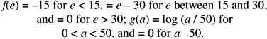
This model has the property that for fixed attained age, the ERR/Sv is constant (at different levels) for exposure ages less than 15 years and greater than 30, but decreases between ages 15 and 30; the estimated ERR/Sv for ages less than 15 years is about 2.2 times that for ages greater than 30. For fixed exposure ages, the ERR/Sv declines up to an attained age of 50 and then remains constant; the ERR/Sv for attained age 30 is about 2.3 times that at attained age 50 or more. This model was chosen because it provided a slightly better fit to the data than a model that allowed risks to vary over the full range of exposure and attained ages [i.e., f(e) = e − 30; g(a) = log (a / 50)] and because it allowed more statistically stable estimates at the extremes of the exposure ages and attained ages.
The parameters ![]() , γ, and η were estimated from an analysis of all solid cancers excluding thyroid and nonmelanoma skin cancer, although cancers that occur in only one sex were excluded in estimating N; the estimated values of
, γ, and η were estimated from an analysis of all solid cancers excluding thyroid and nonmelanoma skin cancer, although cancers that occur in only one sex were excluded in estimating N; the estimated values of ![]() , γ, and η were, respectively, 0.84, −0.053, and −1.63. For cancer of a specific site, only data for that site were used to estimate β, and an approach similar to that used by Pierce and colleagues (1996) and by UNSCEAR (2000b) was used to estimate the parameters
, γ, and η were, respectively, 0.84, −0.053, and −1.63. For cancer of a specific site, only data for that site were used to estimate β, and an approach similar to that used by Pierce and colleagues (1996) and by UNSCEAR (2000b) was used to estimate the parameters ![]() , γ, and η. With this approach, the common values noted above were used unless there was evidence that the site-specific values differed significantly from these common values. In the NIH application, the common values of γ and 0 were used for all specific sites other than lung and the category female genital cancers other than ovary, where these parameters were set equal to zero. The common value for
, γ, and η. With this approach, the common values noted above were used unless there was evidence that the site-specific values differed significantly from these common values. In the NIH application, the common values of γ and 0 were used for all specific sites other than lung and the category female genital cancers other than ovary, where these parameters were set equal to zero. The common value for ![]() was used for all sites except liver cancer, where the ERR/Sv for the two sexes was assumed to be equal; this choice was based on an analysis of liver cancer by Cologne and colleagues (1999). The assessment of uncertainty in the estimated parameters, some of which were site-specific and some of which were common to several sites, was complex and made use of an approach known as joint analysis (Pierce and Preston 1993); joint analysis allows some parameters to depend on cancer site whereas others are assumed to be common to several sites.
was used for all sites except liver cancer, where the ERR/Sv for the two sexes was assumed to be equal; this choice was based on an analysis of liver cancer by Cologne and colleagues (1999). The assessment of uncertainty in the estimated parameters, some of which were site-specific and some of which were common to several sites, was complex and made use of an approach known as joint analysis (Pierce and Preston 1993); joint analysis allows some parameters to depend on cancer site whereas others are assumed to be common to several sites.
Although the models for solid cancer ERRs were based on linear dose-response functions, these estimates were reduced by a DDREF for estimating risks at low doses and low dose rates. Uncertainty in the DDREF was reflected in distributions that included values ranging from 0.5 to 5; different distributions were used for breast and thyroid cancer (more weight was given to linearity for these cancers). The DDREF is applied to all chronic exposures, whereas for acute exposures, the DDREF is phased in as the dose is decreased.
The NIH undertook a comprehensive uncertainty assessment. In fact, uncertainty was a fundamental part of the process in that the emphasis was not on determining single point estimates, but on estimating the uncertainty distribution. Uncertainty distributions for each of several sources were developed and Monte Carlo simulations were carried out to obtain overall uncertainty distributions for both the estimated ERR and the assigned share. A software tool Interactive RadioEpidemiological Program (IREP) was developed to carry out the simulations. Output from IREP gives several percentiles of the distribution for both the ERR and the assigned share. The following uncertainty sources were in-
cluded: sampling variability in the estimated ERRs (including uncertainty in parameters expressing modification by age at exposure, sex, etc.), correction for random and systematic errors in A-bomb survivor dosimetry, extrapolation of risk from high to low doses and low dose rates (expressed as uncertainty in the DDREF), transfer of risk estimates from A-bomb survivors to a U.S. population, and modification by smoking history (lung cancer only). With the exception of sampling variability, the uncertainty distributions for the individual sources were based on informed but nevertheless subjective judgments.
ANNEX 12B: COMMITTEE ANALYSES OF DATA ON THE LSS COHORT TO DEVELOP BEIR VII MODELS FOR ESTIMATING CANCER RISKS
Chapter 12 describes models that were used by the committee to estimate cancer risks. These models were based primarily on analyses of A-bomb survivor cancer incidence data (1958–1995) and, to a lesser extent, mortality data (1950–1997), with consideration of published analyses of data from selected studies involving medical exposures. This annex presents details of analyses of data from the LSS cohort of atomic bomb survivors that were conducted to develop these models. Analyses of cancer mortality data were conducted by the committee. Because the most recent cancer incidence data were not yet available outside of RERF, analyses of these data were conducted under the direction of the committee by RERF investigators who served as agents of the Academy.
The committee’s selected models for estimating solid cancer risks allow the ERR or EAR to depend on both age at exposure and attained age. Both the ERR and the EAR decline with increasing age at exposure. The ERR also declines with increasing attained age, while the EAR increases with increasing attained age. The BEIR VII models are similar to the model used in recent analyses of atomic bomb survivor data by RERF investigators, except that with the BEIR VII model, the ERR and EAR decrease with age at exposure only over the range 0–30 years with no further decrease after age 30. The material that follows describes analyses that were conducted to evaluate several possible models for solid cancer risks, including models that allow for dependence on age at exposure alone, on attained age alone, on time since exposure instead of attained age, and on the use of different functional forms to express these dependencies. Also evaluated are several models for leukemia risks.
Aproach to Analyses
Analyses of cancer incidence were based on cases diagnosed in the period 1958–1998. Analyses of mortality from all solid cancers and from leukemia were based on deaths occurring in the period 1950–2000 (Preston and others 2004), whereas analyses of mortality from cancer of specific sites were based on deaths occurring in the period 1950–1997 (Preston and others 2003). Both ERR models and EAR models were evaluated. Methods were generally similar to those used in recent reports by RERF investigators (Pierce and others 1996; Preston and others 2003) and were based on Poisson regression using the AMFIT module of the software package EPICURE (Preston and others 1991). Confidence intervals (95%) were usually calculated as the estimate plus and minus 1.96 times the standard error. For estimates of linear coefficients of dose, these were calculated on a logarithmic scale. Occasionally (as noted) confidence intervals were calculated using the likelihood profile. All p-values were based on chi-square approximations of likelihood ratio tests. These are based on differences in the maximized log likelihood statistics, often referred to as deviances.
To fit ERR models, baseline risks were handled by stratifying on gender, city of exposure (Hiroshima or Nagasaki), age at exposure, and attained age as described by Pierce and colleagues (1996). To fit EAR models, baseline risks were modeled using the parametric model described by Preston and coworkers (2003). For leukemia, the parametric model is that described by Preston and coworkers (2004). The risk of radiation-induced cancer was modeled as described in the sections that follow.
All analyses were based on newly implemented DS02 dose estimates. Doses were expressed in sieverts with a constant weighting factor of 10 for the neutron dose; that is, the doses were calculated as γ-ray absorbed dose (grays) + 10 × neutron absorbed dose (grays). Analyses were adjusted for random errors in doses using an approach described by Pierce and colleagues (1990) and developed from DS86 dose estimates. Preston and colleagues (2004) note that it has not yet been determined if modification of these methods is needed for DS02 dose estimates. Unless stated otherwise, doses are truncated to correspond to the 4 Gy kerma level.
The DS02 system provides estimates of doses to several organs of the body. For site-specific cancers the committee used dose to the organ being evaluated, with colon dose used for the residual category of “other” cancers. The weighted dose, d, to the colon was used for the combined category of all solid cancers or all solid cancers excluding thyroid and nonmelanoma skin cancer. This choice was made to achieve comparability with analyses by RERF investigators. Reference to an average organ dose—approximated, say, by the dose to the liver—might be more realistic for the analysis of solid cancers combined and would likely lead to about a 10% increase in the values of the weighted dose, d, and thus a reduction of about 10% in the risk coefficients (Kellerer and others 2001). However, the committee’s estimates of the risk for all solid cancers are obtained by summing estimates for individual organ sites (based on doses to these organs), and thus should not be subject to this bias.
It has also been suggested that a weighting factor of roughly 30 for the neutron absorbed dose might be a better
choice than 10. The higher value corresponds more closely to the radiation weighting factor recommended by the ICRP (1991) for fission neutrons. However, with the higher value it becomes critical that the weighting factor stands for the neutron low-dose RBE (i.e., the ratio of the linear coefficients in the dose relations for neutrons and for γ-rays). The weighted dose, d, is then relevant only to the linear term in the dose-effect relation, while the dose-square term, which corresponds to a DDREF, has to contain the γ-ray absorbed dose alone. This change in the analysis might, in the case DDREF = 1, reduce the estimated ERR/Sv by roughly another 15% (Kellerer and others 2001).
General Considerations in Describing Dependencies of Solid Cancer Risks on Exposure Age and Attained Age
A decline in the solid cancer ERR with increasing exposure age has been demonstrated in several epidemiologic studies (UNSCEAR 2000b), and most models for estimating risks of solid cancers in the last decade have included a term that allowed for such a decline. Analyses of A-bomb survivor incidence and mortality data from the recent past (Thompson and others 1994; Pierce and others 1996) emphasized models of the form
(12B-1)
where D is dose in sieverts, βM and βF are sex-specific estimates of the ERR/Sv for exposure at age 30, and e is age at exposure in years. This model is often parameterized so that the βs are the risks at an exposure age of 30, that is, by replacing e by (e − 30).
Although allowing for dependence of the ERR on exposure age seems appropriate, quantifying this dependence is subject to considerable uncertainty, especially for cancers of specific sites. Most medically exposed cohorts involve limited ranges of exposure age, and there is no medically exposed cohort that covers the full range of exposure ages from early childhood to old age. Thus, statistical power for evaluating the effects of exposure age within any single cohort is usually low.
The LSS cohort of Japanese A-bomb survivors is unique in providing data on persons exposed at all ages and, for this reason, has been used in many past risk assessments to quantify the effects of age at exposure (BEIR V, UNSCEAR). Reasonably precise estimates can be obtained when all solid cancers are analyzed as a single outcome. However, sample sizes for individual cancer sites are usually too small to quantify the effects of exposure age precisely. Estimates of the parameter γ vary widely among sites, but it is not possible to determine the extent to which this variation reflects real differences and the extent to which it reflects statistical variation.
An additional problem in quantifying the effect of age at exposure is that since all A-bomb survivors were exposed at the same time, the effects of exposure age are confounded with birth cohort effects. Japanese baseline rates for cancers of many specific sites show strong secular trends, which probably result at least in part from changes in life-style that have come about with the Westernization of Japan. For example, baseline rates for cancers of the colon, lung, and female breast have increased over the past 50 years so that early birth cohorts have lower baseline risks than later birth cohorts. This means that the appropriate way to estimate the effects of exposure age depends on how the factors responsible for secular trends affect radiation risks. If these factors increase or decrease radiation risks to the same extent that they increase or decrease baseline risks (a multiplicative relationship), then estimation of the effect of age at exposure should be based on modeling the ERR. However, if the factors responsible for secular trends in baseline risks have no effect on radiation risks (an additive relationship), then estimation of the effects of age at exposure should be based on modeling the EAR. If the chosen model is not correct, then estimated exposure age effects may be influenced by secular trends in Japanese baseline rates and may not be applicable to populations other than the LSS cohort. Further discussion of secular trends and their influence on estimating the effects of age at exposure can be found in Preston and colleagues (2003).
With the Equation (12B-1) model, the ERR is assumed to be constant over the follow-up period for fixed exposure age. (This is likely to be an oversimplification since Little and others 1991, Thompson and others 1994, and Pierce and others 1996 have all demonstrated that the ERR declines with increasing attained age, or time since exposure, at least for those exposed early in life [under age 20]). In addition, it is now recognized that some and perhaps all of the decline in the ERR with exposure age can also be described as a decline in the ERR with attained age (Kellerer and Barclay 1992; Preston and others 2002a). Pierce (2002) describes the age-time patterns in A-bomb survivor cancer incidence data and discusses difficulties in interpreting them. He also discusses a possible biological rationale for a model in which the ERR decreases with attained age.
As noted in Annex 12A, UNSCEAR (2000b) provided two solid cancer models—one based on age at exposure (as shown by Equation (12B-1)) and one based on attained age. The UNSCEAR attained-age model is of the form
(12B-2)
where D is dose in sieverts, βM and βF are sex-specific estimates of the ERR/Sv, and a is attained age in years. This model is often parameterized so that βs represents the ERR/Sv at attained age 60, that is, by replacing a by (a / 60).
Even when the exposure-age and attained-age models provide comparable fits to the data, estimated lifetime risks based on the two models are not the same, especially for specific age-at-exposure groups such as persons exposed
early in life. For example, UNSCEAR estimates for persons exposed at age 10 based on the exposure-age model are about twice those based on the attained-age model.
The most recent analyses of A-bomb survivor incidence (R13 incidence report) and mortality data (Preston and others 2003) have emphasized models that allow the ERR to depend on both age at exposure and attained age. That is,
(12B-3)
This choice was made in part because of difficulties in distinguishing the fits of the two models above and because, with the incidence data, analyses of all solid cancers indicated a need for modification by both exposure age and attained age. It is expected that analyses of updated cancer incidence data will allow for dependencies on both exposure age and attained age.
Recent A-bomb survivor reports also show results based on models for the EAR. These models are of the same form as given above, although the parameters have different interpretations. In particular, the parameter that quantifies the dependence on attained age describes the strong increase in excess risk with this variable.
The models developed in the following two sections allow for dependencies on both exposure age and attained age. Although the RERF model is evaluated, consideration has also been given to other forms for the dependencies on exposure age and attained age. Both ERR and EAR models are evaluated. Because sample sizes for individual cancer sites are usually too small to quantify precisely the effects of either age at exposure or attained age, the parameters that quantify these effects are in most cases obtained from analyses of all solid cancers. As shown later, with ERR models there are few instances in which the site-specific estimates of these parameters differ significantly from the common values. However, with EAR models there is evidence that the dependence on attained age varies by site.
In the material that follows, the committee first describes analyses conducted to determine the basic form of the preferred model. It then describes analyses of site-specific cancers that were used to confirm the committee’s model choice and to evaluate the appropriateness of using common parameters.
Analyses of Incidence Data on All Solid Cancers Excluding Thyroid and Nonmelanoma Skin Cancer and of Mortality Data on All Solid Cancers
The analyses of cancer incidence data described in this section were based on the category of all solid cancers excluding thyroid cancer and nonmelanoma skin cancer. These exclusions were made primarily because both thyroid cancer and nonmelanoma skin cancer exhibit exceptionally strong age dependencies that do not seem to be typical of cancers of other sites (Thompson and others 1994). With the incidence data, there were 12,778 solid cancer cases occurring in the periods 1958–1998 after the exclusion of 401 thyroid cancers and 275 nonmelanoma skin cancers. Because the most recent mortality data (1950–2000) available to the committee did not include site-specific solid cancer, analyses of mortality data were based on all solid cancers (including thyroid and nonmelanoma skin cancer). There were 10,127 solid cancer deaths occurring in the period 1950–2000. The number of thyroid and nonmelanoma skin cancers included in this group is likely to have been small. Of the 9399 solid cancer deaths occurring in the period 1950–1997 (Preston and others 2003), only 64 (0.7%) were due to thyroid cancer and 32 (0.3%) to nonmelanoma skin cancer. Table 12B-1A shows the distribution of cases (1958–1998) and deaths (1950–2000) by sex and dose category. Table 12B-1B shows the distribution of site-specific cancers by sex, with the num-
TABLE 12B-1A Number of Incidence Cases of Solid Cancer Excluding Thyroid and Nonmelanoma Skin Cancer and Number of Deaths from Solid Cancer by Sex and Colon Dose
|
Colon Dose (Sv) |
No. of Cases (1958–1998) |
No. of Deaths (1950–2000) |
||||
|
Males |
Females |
Total |
Males |
Females |
Total |
|
|
< 0.005 |
2,504 |
2,855 |
5,359 |
2,089 |
2,181 |
4,270 |
|
0.005–0.1 |
1,900 |
2,295 |
4,195 |
1,603 |
1,784 |
3,387 |
|
0.1–0.2 |
379 |
547 |
926 |
307 |
425 |
732 |
|
0.2–0.5 |
473 |
602 |
1,075 |
379 |
436 |
815 |
|
0.5–1.0 |
294 |
348 |
642 |
241 |
242 |
483 |
|
1.0–2.0 |
199 |
219 |
418 |
160 |
166 |
326 |
|
2.0 + |
74 |
89 |
163 |
51 |
63 |
114 |
|
Total |
5,823 |
6,955 |
12,778 |
4,830 |
5,297 |
10,127 |
TABLE 12B-1B Number of Incidence Cases and Number of Deaths by Cancer Site and Sex
|
Cancer Site |
No. of cases (1958–1998) |
No.of Deaths (1950–1997) |
||||
|
Males |
Females |
Total |
Males |
Females |
Total |
|
|
Stomach |
1,899 |
1,703 |
3,602 |
1,555 |
1,312 |
2,867 |
|
Colon |
547 |
618 |
1,165 |
206 |
272 |
478 |
|
Liver |
676 |
470 |
1,146 |
722 |
514 |
1,236 |
|
Lung |
770 |
574 |
1,344 |
716 |
548 |
1,264 |
|
Breast |
7 |
847 |
854 |
3 |
272 |
275 |
|
Prostate |
281 |
0 |
281 |
104 |
0 |
104 |
|
Ovary |
0 |
190 |
190 |
0 |
136 |
136 |
|
Uterus |
0 |
875 |
875 |
0 |
518 |
518 |
|
Bladder |
227 |
125 |
352 |
83 |
67 |
150 |
|
Other solid |
1,416 |
1,553 |
2,969 |
1,036 |
1,175 |
2,211 |
|
Total |
5,823 |
6,955 |
12,778 |
4,425 |
4,814 |
9,239 |
ber of deaths based on the period 1950–1997 rather than 1950–2000, the period used in Table 12B-1A.
The following general linear dose-response function was used to model the ERR or EAR:
(12B-4)
where D is dose in sieverts, βM and βF are sex-specific estimates of the ERR/Sv, e is age at exposure in years, and a is attained age in years. The function h includes parameters to be estimated. Most commonly, h is of the form
(12B-5)
As noted above, recent analyses by RERF investigators of A-bomb survivor solid cancer mortality (Preston and others 2003) and incidence data have taken f(e) = e and g(a) = log a; note that exp (η log a) = aη. Others (Kellerer and Barclay 1992) have developed models with g(a) = a.3 Some past risk assessments (BEIR V) have taken h to be a function of sex, age at exposure, and time since exposure (t). Note that any two of the variables e, a, and t determine the third (t = a − e) so models based on e and t are included in the equation (12B-4) specification.
In recent analyses conducted for the purpose of updating radioepidemiologic tables (NIH 2003), the NIH evaluated models of the form indicated above, but the ERR was allowed to vary over only a limited range of exposure ages or attained ages. The models evaluated by the NIH included those in which the ERR varied with age at exposure only over the ranges 0–30 and 15–30 years, and in which the ERR varied with attained age only over the range 0–50 years. Stated mathematically, these models for age at exposure are as follows:
where min = minimum and max = maximum. Note that the variable e_u30 is equal to e − 30 for e < 30, and equal to zero for older ages. That is, it allows for modification of the ERR for exposure ages between 0 and 30, but allows no further modification after age 30. The variable e_15to30 allows the ERR to change over the interval 15–30 years, whereas the ERR is constant (at different levels) for exposure ages under 15 or over 30. As seen later, e_u30 is selected for use in the committee’s preferred models. Thus, the simpler notation e* = e_u30 is introduced.
The alternative for attained age was
The variable log (a)_u50 allows for modification of the ERR for attained ages under 50, but allows no further modification after age 50. The final model used in the NIH report (2003) was based on e_15to30 and log (a)_u50. With the LSS cancer incidence data available at the time (1958–1987), these choices gave a slightly better fit to the data than the alternatives that were evaluated.
To decide on the preferred BEIR VII model, the committee evaluated several alternative choices for f(e) and g(a) using data both on incidence of all solid cancers excluding thyroid cancer and nonmelanoma skin cancer and on mortality from all solid cancers. The committee conducted a series of analyses of all solid cancers excluding thyroid cancer and nonmelanoma skin cancer with several alternative choices for f(e) and g(a); it also evaluated models based on time since exposure instead of attained age. As noted earlier, in fitting ERR models, baseline risks were handled by stratifying on sex, city of exposure (Hiroshima or Nagasaki), age at exposure, and attained age as described by Pierce and colleagues (1996). More limited analyses were conducted using an EAR model with the same form as the ERR model. To fit the EAR models, it was necessary to use a parametric baseline. The committee used a similar parametric model to that described by Preston and colleagues (2003). To evaluate comparability with stratified results, a limited number of parametric ERR models were also fitted.
Table 12B-2 shows the drop in deviance for each of the models compared to a model with no modification by age at exposure, attained age, or time since exposure; such a model is not realistic but facilitates comparison among models. The deviance differences, which follow (approximately) chi-square distributions with the number of degrees of freedom indicated, can be regarded as a measure of the improvement in fit brought about by use of the indicated function of e, a, and t. In general, the greater the deviance difference, the better is the fit of the model. Comparison of these deviance differences is most appropriate among models based on the same data and of the same type (e.g., comparisons among stratified ERR models for incidence data).
All models were of the form indicated in Equation (12B-5), and most (models 1–13) were ERR models with a stratified background. Model 1 is the RERF model given by Equation (12B-3), while models 2 and 3 included only one of the variables e or log (a). With the incidence data, the RERF model fitted the data significantly better than model 2 with only e (p < .001) or model 3 with only log (a) (p = .013). With the updated incidence data, models that include only exposure age (or a function of exposure age) or only attained age (or a function of attained age) do not provide an adequate fit to the data. With the mortality data, the RERF model fitted the data slightly better than model 2 with only e (p = .08), and much better than model 3 with only log (a) (p < .001).
Models 4–6 were addressed at evaluating alternative choices for f(e) and g(a), specifically the alternatives that
TABLE 12B-2 Comparison of Fits of Several Models (As Measured by the Deviance): Estimated Parameters and Deviances for Several Models Expressing Dependence of Risk of Solid Cancer Incidence and Mortality on Age at Exposure (e), Attained Age (a), and Time Since Exposure (t)a
|
Model Number |
Model Typeb |
f(e) |
g(a) or g(t) |
Difference in Deviance for This Model and Model with No Modifiers (degrees of freedom) |
|
|
Incidence Datac |
Mortality Datad |
||||
|
1-RERF |
ERR-S |
e |
log (a) |
50.2 (2) |
37.2 (2) |
|
2 |
ERR-S |
E |
None |
32.9 (1) |
34.2 (1) |
|
3 |
ERR-S |
None |
log (a) |
44.0 (1) |
17.5 (1) |
|
4–BEIR VII |
ERR-S |
e*e |
log (a) |
53.1 (2) |
40.2 (2) |
|
5 |
ERR-S |
e* |
None |
39.4 (1) |
38.1 (1) |
|
6 |
ERR-S |
e_15to30f |
log (a) |
48.1 (2) |
33.8 (2) |
|
7 |
ERR-S |
e* |
log (a)_u50g |
49.2 (2) |
39.1 (2) |
|
8 |
ERR-S |
e* |
a |
51.4 (2) |
40.2 (2) |
|
9 |
ERR-S |
e* |
t |
51.1 (2) |
39.4 (2) |
|
10 |
ERR-S |
e* |
log (t) |
49.1 (2) |
38.5 (2) |
|
11 |
ERR-S |
e |
a |
48.2 (2) |
37.1 (2) |
|
12 |
ERR-S |
e |
t |
48.2 (2) |
37.1 (2) |
|
13 |
ERR-S |
e |
log (t) |
46.3 (2) |
35.6 (2) |
|
1B-RERF |
ERR-P |
e |
log (a) |
50.55h (2) |
37.0i (2) |
|
4B-BEIR VII |
ERR-P |
e* |
log (a) |
53.85 (2) |
41.1 (2) |
|
1C-RERF |
EAR-P |
e |
log (a) |
80.34h (2) |
113.0i (2) |
|
4C-BEIR VII |
EAR-P |
e* |
log (a) |
84.21 (2) |
115.5 (2) |
|
aBased on models in which the ERR or EAR is given by βsD exp [γ e* + η log (a / 60)]. bERR-S: stratified excess relative risk model; ERR-P: parametric excess relative risk model; EAR-P: parametric excess absolute risk model. cBased on analyses of solid cancers excluding thyroid and nonmelanoma skin cancers, 1958–1998 (12,778 incident cases). dBased on analyses of all solid cancers, 1950–2000 (10,127 deaths). ee* is (e − 30) / 10 for e < 30 and zero for e 30, where e is age at exposure in years. fe; e_15to30 is −1.5 for e < 15, (e − 30) / 10 for e between 15 and 30, and 0 for e 30, where e is exposure age in years. glog (a)_u50 = log (a / 50) for a < 50 and 0 for a 50, where a is attained age in years. hThe deviance based on incidence data for model 4B was 20,377.0; that for model 4C was 20,388.3. iThe deviance based on incidence data for model 4B was 13,766.8; that for model 4C was 13,769.0. |
|||||
were evaluated by NIH (2003). Of these choices, model 4 resulted in the best fit (greatest deviance difference) for both incidence and mortality data, although differences between models 1 and 4 were not great. This model allows for variation in the ERR with age at exposure only over the range 0 to 30 years, but allows for variation in attained age over the full range. The model, which is as follows,
(12B-6)
is referred to as the BEIR VII ERR model. With the incidence data, the BEIR VII ERR model fitted the data significantly better than model 3 with only log (a) (p = .0025) or model 5 with only e* (p < .001). With the mortality data, this model fitted the data much better than model 3 with only log (a) (p < .001), and slightly better than model 5 with only e* (p = .15). With both incidence and mortality data, the BEIR VII model fitted the data somewhat better than the RERF model. Comparison of the BEIR VII model with model 6 indicates that e* is a better choice than e_15to30 (particularly for the mortality data), whereas comparison with model 7 indicates that log (a) is a slightly better choice than log (a)_u50. However, the fits of models 1, 4, and 7 do not differ greatly.
The committee also evaluated the use of a, t, and log (t) as substitutes for log (a) in models that also included e* (respectively, models 8, 9, and 10) or that also included e30 (models 11, 12, and 13). None of these models fitted the data as well as the BEIR VII model, although the differences were not great. Models 11 and 12 are different parameterizations of the same model.
For reasons that are discussed later in this annex, the committee fitted models that added exposure age variables e_over30 = max (0, e − 30) and e_over55 = max (0, e − 55). When e_over30 was added to the BEIR VII model, the estimated coefficients were positive. There was little evidence of improvement in fit (p > .50 for both incidence and mortality data), but this shows that there is no evidence of a decline in risk after age 30. However, with the incidence data, when e_over55 was added to the BEIR VII model, the p-value for improvement in fit was .044; when added to the RERF
model, the p-value was .015. The e_over55 parameter was positive, indicating an increase in risks for those exposed at older ages. This finding is discussed later in this section. For now, note only that there is no evidence that risks continue to decline for exposure ages greater than 30; thus, the BEIR VII model seems a better choice than the RERF model. With mortality data, there was little indication that adding e_over55 improved the fit (p = .46).
The committee also evaluated whether using sex-specific estimates of the modifying effects of e*_u30 or log (a) would substantially improve the fit of the BEIR VII model. There was no evidence of improvement in fit with the sex-specific model (p > .5 for both incidence and mortality) resulting in a deviance of 11,825.63, only slightly lower than model 1 (difference in deviances = 1.10; p > .5).
Models 1B and 4B were comparable to models 1 and 4 except that they were based on parametric modeling of the baseline risks. The estimated coefficients were similar to those obtained for the comparable models 1 and 4 based on stratified ERR models. These analyses also support the use of e* instead of e.
Models 1C and 4C are EAR models. Model 1C has the same functional form as the RERF model shown in Equation (12B-3), whereas model 4C has the same functional form as the BEIR VII model shown in Equation (12B-6). The same variables were used to model the baseline risk as in respective models 1B and 4B. Again, model 4C (with e*) provides a somewhat better fit than does model 1C (with e). The deviances for the ERR models are slightly lower than the corresponding EAR models. Model 1C is subsequently referred to as the “RERF ERR model,” and model 4C as “the BEIR VII EAR model.”
As another approach to evaluating alternative models, separate ERRs per sievert and EARs per 104 PY-Sv were estimated for each of five groups defined by age at exposure (<15, 15–30, 30–45, 45–60 and 60+ years). That is, the following model was fitted:
(12B-7)
where j indexes the five age-at-exposure categories. The estimated βjs, averaged for the two sexes, are shown in Table12B-3. For both incidence and mortality data, we see the expected decline in risk for exposure ages under 60, with a stronger decline for mortality data than for incidence data. Somewhat surprisingly, the estimates for the 60+ exposure age group are three to four times those in the next-oldest age group for the incidence data, and about twice those in next-oldest age group for the mortality data. The difference between the coefficients βj for the two oldest age-at-exposure groups was statistically significant for the incidence data (p = .04 for the ERR model; p = .03 for the EAR model) but not for the mortality data (p > .3). Because there was not an a priori hypothesis that the ERR/Sv would increase for the oldest exposure age category, a more appropriate test may be to compare the deviance for the BEIR VII model shown in Equation (12B-6) to that of the model shown below:
(12B-8)
in which the single parameter β is replaced by five separate parameters for the five age-at-exposure categories. This four-degree-of-freedom test resulted in p-values that exceeded .15 for the incidence data and exceeded .45 for the mortality data.
Further exploration of the cancer incidence data revealed that the elevation of both ERR and EAR for the oldest exposure age category was strongest for stomach and liver cancers; for these cancers, βjs for the 60+ exposure age group
TABLE 12B-3 Sex-Averaged Estimates of ERR/Sv and EAR per 104 PY-Sv by Age-at-Exposure Categories for All Solid Cancers Excluding Thyroid and Nonmelanoma Skina
|
Data Used |
Age at Exposure |
||||
|
<15 years |
15–30 years |
30–45 years |
45–60 years |
60+ years |
|
|
Incidence datab |
|||||
|
Number of cases |
2044 |
3465 |
4417 |
2526 |
326 |
|
ERR/Sv (95% CI) |
0.78 (0.58, 1.06) |
0.63 (0.49, 0.81) |
0.42 (0.28, 0.62) |
0.43 (0.23, 0.79) |
1.7 (0.76, 3.8) |
|
EAR per 104 PY-Sv (95% CI) |
57 (43, 76) |
40 (30, 48) |
23 (16, 33) |
20 (11, 36) |
67 (35, 131) |
|
Mortality datac |
|||||
|
Number of deaths |
1220 |
2188 |
3679 |
2572 |
468 |
|
ERR/Sv (95% CI) |
1.12 (0.80, 1.58) |
0.63 (0.46, 0.84) |
0.35 (0.22, 0.55) |
0.25 (0.10, 0.55) |
0.55 (0.19, 1.7) |
|
EAR per PY-Sv (95% CI) |
29 (21, 39) |
18 (14, 25) |
12 (7.9, 19) |
8.4 (3.7, 19) |
17 (6.1, 45) |
|
aBased on models in which the ERR or EAR is of the form βj [1 + θ s] D exp [η log (a)], where j indexes age-at-exposure categories, s is sex, and a is attained age in years. bBased on solid cancers excluding thyroid and nonmelanoma skin cancers, 1958–1998. cBased on all solid cancers, 1950–2000. |
|||||
were more than eight times those for the 45–60 exposure age group (p = .02), while for the remaining solid cancers this ratio was less than 2 and did not differ significantly from unity (p > .5).
The increased ERR/Sv and EAR per 104 PY-Sv for the oldest age-at-exposure group was one of the reasons the committee selected the BEIR VII model with no decline with exposure age after age 30 in preference to the RERF model with a decline throughout the entire range of exposure age. The committee notes particularly that stomach and liver cancers, for which this effect was strongest, are far more prevalent in Japan than in the United States. With the incidence data, about 37% of the cancers in the solid cancer category that the committee analyzed were cancers of the stomach and liver; by contrast, SEER data for the United States (see Table 12-3) indicate that only about 3% of incident cancers are of these types. Furthermore, risks for stomach and liver cancers may be affected by infectious agents such as Helicobacter pylori for stomach cancer and the hepatitis virus for liver cancer (Parsonnet and others 1994; Aromaa and others 1996; Goldstone and others 1996). Infection rates might differ by birth cohort (and thus exposure age), which could affect risks due to radiation in ways that are not currently understood. Although the reason for the relatively high ERR/Sv among those exposed at older ages is not fully understood the committee does not think that this effect is likely to generalize to a modern U.S. population.
Based on the analyses of A-bomb survivor data described above, the committee has selected the model shown in Equation (12B-6) as its preferred model for estimating solid cancer risks. However, several alternative choices, including the RERF model shown in Equation (12B-3), fitted the data nearly as well and would also have been reasonable choices. Both ERR and EAR models are evaluated. Table 12B-4 shows the estimated parameters (with 95% confidence intervals) for ERR and EAR models obtained from both incidence and mortality data. With the ERR models, the effect of exposure age is stronger for mortality than for incidence data, while the effect of attained age is weaker. The two EAR models show similar exposure age effects, but the rate of increase with attained age is greater for the mortality data than for the incidence data.
The committee also evaluated mortality data on all solid cancers to compare the use of 5- and 10-year minimal latent periods. This was done by fitting the BEIR VII ERR model, and estimating the ERR/Sv separately for the period 5–9 years following exposure and for the period 10 or more years following exposure. Although the estimate for the 5–9-year period was not quite statistically significant with a two-sided test (p = .10), there was no evidence that it differed from the estimate for the later follow-up period (p = .44). The committee accordingly has used a minimal latent period of 5 years in its calculations of lifetime risks.
TABLE 12B-4 ERR and EAR Models for Estimating Incidence of All Solid Cancers Excluding Thyroid and Nonmelanoma Skin Cancers and Mortality from All Solid Cancersa,b
|
ERR Models |
No. of Cases or Deaths |
ERR/Sv (95% CI) at Age 30 and Attained Age 60 |
Per-Decade Increase in Age at Exposure Over the Range 0–30 Yearsc (95% CI), γ |
Exponent of Attained Age (95% CI), η |
|
|
Males (βM) |
Females (βF) |
||||
|
Incidenced |
12,778 |
0.33 (0.24, 0.47) |
0.57 (0.44, 0.74) |
−0.30 (−0.51, −0.10) |
−1.4 (−2.2, −0.7) |
|
Mortalitye |
10,127 |
0.23 (0.15, 0.36) |
0.47 (0.34, 0.65) |
−0.56 (−0.80, −0.32) |
−0.67 (−1.6, 0.26) |
|
EAR models |
|
EAR per 104 PY-Sv (95% CI) |
|
||
|
Males (βM) |
Females (βF) |
||||
|
Incidenced |
12,778 |
22 (15, 30) |
28 (22, 36) |
−0.41 (−0.59, −0.22) |
2.8 (2.15, 3.41) |
|
Mortalitye |
10,127 |
11 (7.5, 17) |
13 (9.8, 18) |
−0.37 (−0.59, −0.15) |
3.5 (2.71, 4.28) |
|
NOTE: Estimated parameters with 95% CIs. PY = person-years. aThe ERR or EAR is of the form βsD exp (γe*) (a / 60)η, where D is the dose (Sv), e is age at exposure (years), e* is (e − 30) / 10 for e < 30 and zero for e 30, and a is attained age (years). bThe committee’s preferred estimates of risks from all solid cancers are obtained as sums of estimates based on models for site-specific cancers (see Table 12-2 and text). cChange in ERR/Sv or EAR per 104 PY-Sv (per-decade increase in age at exposure) is obtained as 1 − exp (γ). dBased on analyses of LSS incidence data 1958–1998 for all solid cancers excluding thyroid and nonmelanoma skin cancer. eBased on analyses of LSS mortality data 1950–2000 for all solid cancers. |
|||||
Analyses of Incidence and Mortality Data on Site-Specific Solid Cancers
Although the committee provides risk estimates for both cancer incidence and mortality, models for site-specific cancers were based mainly on cancer incidence data. This was done primarily because site-specific cancer incidence data are based on diagnostic information that is more detailed and accurate than death certificate data and because, for several sites, the number of incident cases is considerably larger than the number of deaths. For cancers of the colon, breast, prostate, and bladder, the number of cases in the LSS cohort is more than double the number of deaths (Table 12B-1B). In addition, mortality data may be more subject than incidence data to changes over time brought about because of improved survival. Models developed from incidence data were however evaluated for consistency with mortality data. Since there is little evidence that radiation-induced cancers are more rapidly fatal than cancer that occurs for other reasons, ERR models based on incidence data can be used directly to estimate risks of cancer mortality. EAR models require adjustment as discussed in the chapter.
Models for site-specific cancers were based on the BEIR VII model indicated by Equation (12B-6). The committee’s approach to quantifying the parameters γ and η was to use the estimates obtained from analyzing incidence data on all solid cancers excluding thyroid and nonmelanoma skin cancers unless site-specific analyses indicated significant departure from these estimates. Table 12B-5A shows the results of fitting ERR site-specific models to the incidence data. Results are shown for a model in which all four of the parameters βM, βF, γ, and η were estimated and are also shown for a model in which the parameters quantifying the modifying effects of age of exposure and attained age γ and η were set equal to the values obtained from analysis of the category all solid cancers excluding thyroid and nonmelanoma skin cancers; these values are referred to subsequently as the “common values.” The final column gives the deviance difference between the two models and the resulting p-value based on a two-degree-of-freedom test comparing the fits of the two models. This test does not take account of uncertainty in the estimates of the common values of γ and η. In addition, the committee fitted models in which just one of the parameters γ and η was fixed, with the other estimated allowing a one-degree-of-freedom test for each of the parameters.
The only sites with even modest evidence (p < .10) of departure from the fixed values of γ and η were cancer of the uterus and the category “all other solid cancers.” For cancer of the uterus, the estimated ERR/Sv was very small and nonsignificant so that it was not possible to obtain stable estimates of the modifying parameters; thus the common values were used. For other solid cancers, a test for the parameter η alone resulted in a p-value of .025; thus, results are also
TABLE 12B-5A Results of Fitting Stratified ERR Models to Site-Specific Cancer Incidence Data Using the Model ERR(D, s, e, a) = βsD exp [γ e* + η log (a / 60)]a
|
Cancer Site |
No. of Cases |
All Parameters Estimated |
Fixed Parameters: γ = −0.30; η = −1.4 |
Deviance Differenceb (p-value) |
||||
|
βM |
βF |
γ |
η |
βM |
βF |
|||
|
Solid cancerc |
12,778 |
0.33 |
0.57 |
−0.30 |
−1.4 |
0.33 |
0.57 |
|
|
Stomach |
3602 |
0.25 |
0.54 |
−0.13 |
−1.9 |
0.21 |
0.48 |
0.5 (> 0.5) |
|
Colon |
1165 |
0.72 |
0.54 |
−0.16 |
−3.1 |
0.63 |
0.43 |
1.0 (> 0.5) |
|
Liver |
1146 |
0.40 |
0.36 |
−0.15 |
−1.5 |
0.32 |
0.32 |
0.2 (> 0.5) |
|
Lung |
1344 |
0.39 |
1.68 |
0.05 |
−1.1 |
0.32 |
1.40 |
2.9 (0.23) |
|
Breast |
847 |
— |
1.19 |
−0.04 |
−2.0 |
— |
0.91 |
2.4 (0.34) |
|
Prostated |
281 |
— |
— |
— |
— |
0.12 |
— |
— |
|
Uterus |
875 |
— |
0.027 |
−2 |
5.6 |
— |
0.055 |
5.8 (0.055) |
|
Ovary |
190 |
— |
0.47 |
−0.13 |
−1.6 |
— |
0.38 |
0.05 (> 0.5) |
|
Bladder |
352 |
0.51 |
1.62 |
−0.04 |
0.28 |
0.50 |
1.65 |
2.7 (0.26) |
|
Other solid cancers |
2969 |
0.27 |
0.45 |
−0.29 |
−2.8 |
0.33 |
0.51 |
5.0 (0.081) |
|
Other solid cancers (alternative) |
2969 |
0.27 |
0.45 |
Fixed at −0.30 |
−2.8 |
|
|
0.003e (>0.5) |
|
aD is dose (Sv); e* = (e − 30) / 10 for e < 30, where e is age at exposure (years); e* = 0 for e 30; and a is attained age (years). βM and βF are the ERR/Sv for males and females exposed at age 30 at attained age 60, γ is expressed per decade increase in age at exposure over the range 0–30 years, and a is the exponent of attained age. bDifference in deviance for model shown in columns 7 and 8 and model shown in columns 3–6. cSolid cancer excluding thyroid and nonmelanoma skin cancers. dModel with all parameters estimated would not converge. eDifference in deviance for this model and that shown in columns 3–6 in the row immediately above. |
||||||||
shown for an alternative model with η estimated separately for this category.
Table 12B-5B shows results based on mortality data on site-specific cancers. As in Table 12B-5A, columns 3–6 show results with all four of the parameters βM, βF, γ, and η estimated using data on that site alone. Columns 7 and 8 show the results of testing the compatibility of these models with models developed from the incidence data with γ and η fixed as indicated in columns 7 and 8 of Table 12B-5A. Column 7 is based on analyses in which γ was set equal to −0.30 per decade and η was set equal to −1.4, and the parameters βM and βF were estimated, and thus tests whether the fixed values of data γ and η are compatible with the mortality data. Column 8 is based on analyses in which all four of the parameters βM, βF, γ and η were set equal to the values estimated from the incidence data (Table 12B-5A). The alternative model for “all other solid cancers,” based on the incidence data, was also evaluated. Because of difficulties in fitting four-parameter models for cancers of the prostate and uterus, these sites are not shown in Table 12B-4B. Only for colon cancer and for all other solid cancers was there a suggestion (p < .10) that the models based on incidence data did not fit the mortality data. Because there was no evidence against using the common values of η and γ for colon cancer based on the incidence data, the committee chose to use the common values for this site. For all other solid cancers, the alternative model developed from the incidence data was also more compatible with the mortality data, and this was chosen as the preferred model.
Table 12B-5C shows results of fitting EAR models to the cancer incidence data and is analogous to Table 12B-5A for the ERR models. There is clear evidence that common values of the parameters γ and η are not appropriate for cancers of lung, breast, and bladder. For all three of these sites, and also for liver cancer (see below), alternative models in which η was estimated and γ was set at the common value (−0.41) provided acceptable fits.
For breast cancer, the committee fitted additional EAR models with separate parameters for attained ages under 50 and over 50, similar to the model used by Preston and colleagues (2002a) in a pooled analysis of breast cancer incidence data from several cohorts including the LSS data. This model (labeled alternative 2) provided a significantly better fit (p < .001) than did the model with a single parameter for attained age. As discussed in this chapter, the committee’s preferred models for breast cancer were based on pooled analyses by Preston and colleagues (2002a). However, it was of interest to compare these results with those obtained from models based on the same approach as most other cancer sites.
Table 12B-5D shows results of fitting EAR models to the mortality data. All but the last column are analogous to those in Table 12B-4C for the ERR models. The last column of Table 12B-5D shows the deviance differences for models based on the mortality data and the alternative models shown in Table 12B-5C. Only for cancers of the liver, lung, breast, and bladder was there evidence (p < .10) of departure from the main incidence models. However, for these sites, there
TABLE 12B-5B Results of Fitting Stratified ERR Models to Site-Specific Cancer Mortality Data Using the Model ERR(D, s, e, a) = βsD exp [γ e* + η log (a / 60)]a
|
Cancer Site |
No. of Deaths |
All Parameters Estimated |
Fixed Parameters γ = −0.30; η = −1.4 |
||||||
|
βM |
βF |
γ |
η |
βM |
βF |
Deviance Difference for Testing γ and ηb (p-value) |
Deviance Difference for Testing βM, βF, γ, and η (p-value)c |
||
|
Stomach |
2,867 |
0.11 |
0.41 |
−0.65 |
0.29 |
0.14 |
0.46 |
2.6 (0.28) |
3.3 (>0.5) |
|
Colon |
478 |
0.65 |
0.79 |
−0.19 |
−5.3 |
0.68 |
0.68 |
4.8 (0.09) |
5.8 (0.22) |
|
Liver |
1,236 |
0.23 |
0.25 |
−0.51 |
0.82 |
0.28 |
0.29 |
1.8 (0.40) |
2.0 (>0.50) |
|
Lung |
1,264 |
0.36 |
0.80 |
−0.36 |
0.34 |
0.45 |
0.93 |
3.0 (0.23) |
6.6 (0.16) |
|
Breast |
272 |
— |
0.56 |
−0.72 |
−1.5 |
— |
0.94 |
1.9 (0.38) |
2.0 (>0.5) |
|
Ovary |
136 |
— |
0.34 |
−0.10 |
−5.1 |
— |
0.65 |
1.3 (> 0.5) |
2.1 (>0.5) |
|
Bladder |
150 |
1.27 |
1.65 |
0.10 |
−0.65 |
0.90 |
1.18 |
3.3 (0.20) |
3.8 (0.44) |
|
All other solid cancers |
2,211 |
0.24 |
0.30 |
−0.68 |
−1.7 |
0.35 |
0.53 |
5.1 (0.079) |
5.1 (0.28) |
|
All other solid cancer (alternative) |
|
Fixed at −0.30 |
Fixed at −2.8 |
0.32 |
0.44 |
3.3 (0.20) |
3.5 (0.48) |
||
|
aD is dose (Sv); e* = (e − 30) / 10 for e < 30, where e is age at exposure (years); e* = 0 for e 30; and a is attained age (years). βM and βF are the ERR/Sv for males and females exposed at age 30 at attained age 60, γ is expressed per decade increase in age at exposure over the range 0–30 years, and η is the exponent of attained age. bDifference in deviance for model shown in columns 7 and 8 (with γ = −0.30 and η = −1.4) and model shown in columns 3–6 (2 degrees of freedom). cDifference in deviance for model shown in columns 7 and 8 of Table 12B-5A and model shown in columns 3–6 of this table (4 degrees of freedom for cancers occurring in both sexes; 3 degrees of freedom for cancers of the breast, prostate, uterus, and ovary). |
|||||||||
TABLE 12B-5C Results of Fitting Parametric EAR Models to Site-Specific Cancer Incidence Data Using the Model EAR(D, s, e, a) = βsD exp [γ e* + η log (a / 60)]a
|
Cancer Site |
No. of Cases |
All Parameters Estimated |
Fixed Parameters: γ = −4.1; η = 2.8 |
Deviance Differenceb (p-value) |
||||
|
βM |
βF |
γ |
η |
βM |
βF |
|||
|
Solid cancerc |
12,778 |
22 |
28 |
−0.41 |
2.8 |
22 |
28 |
|
|
Stomach |
3,602 |
7.0 |
7.1 |
0.002 |
1.8 |
4.9 |
4.9 |
3.4 (0.18) |
|
Colon |
1,165 |
2.2 |
0.84 |
−1.0 |
5.7 |
3.2 |
1.6 |
4.0 (0.14) |
|
Liver |
1,146 |
1.8 |
0.81 |
−0.64 |
4.8 |
1.9 |
0.83 |
1.9 (0.39) |
|
Liverd (alternative) |
1,146 |
2.2 |
1.0 |
Fixed at −0.41 |
4.1 |
|
|
0.3e (> 0.5) |
|
Lung |
1,344 |
3.1 |
4.6 |
−0.3 |
4.4 |
1.5 |
3.3 |
15.4 (<0.001) |
|
Lung (alternative) |
1,344 |
2.3 |
3.4 |
Fixed at −0.41 |
5.2 |
|
|
2.0e (0.16) |
|
Breast |
847 |
— |
5.6 |
−0.51 |
1.5 |
— |
6.3 |
16.5 (<0.001) |
|
Breast (alternative 1) |
847 |
— |
6.1 |
Fixed at −0.41 |
1.3 |
|
|
0.42e (> 0.5) |
|
Breast (alternative 2) |
847 |
— |
5.9 |
Fixed at −0.41 |
3.4, −2.4f |
|
|
−13.9g (<0.001) |
|
Prostateh |
281 |
— |
— |
— |
— |
0.11 |
— |
— |
|
Uterus |
875 |
— |
0.28 |
−1.6 |
6.3 |
— |
1.2 |
2.7 (0.27) |
|
Ovary |
190 |
— |
0.50 |
−0.66 |
2.7 |
— |
0.7 |
1.2 (> 0.5) |
|
Bladder |
352 |
1.3 |
0.88 |
−0.23 |
5.6 |
1.1 |
0.62 |
6.4 (0.04) |
|
Bladder (alternative) |
352 |
1.2 |
0.75 |
Fixed at −0.41 |
6.0 |
|
|
0.1e (>0.5) |
|
Other solid cancers |
2,969 |
5.1 |
4.2 |
−0.39 |
1.9 |
6.2 |
4.8 |
3.1 (0.22) |
|
aD is dose (Sv); e* = (e − 30) / 10 for e < 30, where e is age at exposure in years; e* = 0 for e 30; and a is attained age in years. βM and βF are the number of excess cases per 104 PY-Sv for males and females exposed at age 30 at attained age 60, γ is expressed per decade increase in age at exposure over the range 0–30 years, and a is the exponent of attained age. bDifference in deviance for model shown in columns 7 and 8 and model shown in columns 3–6. cSolid cancer excluding thyroid and nonmelanoma skin cancers. dThis alternative was developed to obtain a model that was consistent with mortality data. eDifference in deviance for this model and that shown in columns 3–6 in the row immediately above. fThe first coefficient is for attained age under 50; the second coefficient is for attained age over 50. gDifference in deviance for alternative 1 breast model and this model. hModel with all parameters estimated would not converge. |
||||||||
was no evidence of departure from the alternate incidence models. In fact, the alternative liver cancer model was developed because of the large attained age effect identified in the mortality data. In general, the numbers of excess deaths per 104 PY-Sv would be expected to be less than the numbers of excess cases; thus, it was not sensible to evaluate the compatibility of the estimated βM and βF as was done for the ERR models. However, for sites common to both sexes, the committee tested whether or not the ratio βF / βM estimated from the mortality data was compatible with that estimated from the incidence data (with the latter treated as a fixed value). The p-values for the sites tested, based on a single-degree-of-freedom test, were as follows: stomach (p = .19), colon (p = .35), liver (p > .5), lung (p = .28), and all other solid cancers (p > .5).
The analyses of site-specific cancer presented in the last few paragraphs address the use of common parameters to quantify the modifying effects of age at exposure and attained age, but do not address the possibility of common parameters for the overall level of the ERR or EAR (βM and βF). Because at least some of the variation among cancer sites in these estimated parameters is due to sampling variation, one might consider using common parameters for sites where there is no evidence of statistical differences. The committee chose not to use such an approach because it seems likely that there are true differences among the sites and because it was considered desirable to use site-specific data to reflect the uncertainty in site-specific estimates. A promising approach for the future is to use methods that draw both on data for individual sites and on data for the combined category of all solid cancers. With this approach, the variance of the site-specific estimate and the degree of deviation from the all-solid-cancer estimate are considered in developing site-specific estimates that draw both on data for the specific individual site and on data for all solid cancers. The National Research Council (2000) gives a simple il-
TABLE 12B-5D Results of Fitting Parametric EAR Models to Site-Specific Cancer Mortality Data Using the Model EAR(D, s, e, a) = βsD exp [γ e* + η log (a / 60)]a
|
Cancer Site |
No. of Deaths |
All Parameters Estimated |
Fixed Parameters: γ = −4.1; η = 2.8 |
|||||
|
βM |
βF |
γ |
η |
βM |
βF |
Deviance Differenceb (p-value) |
||
|
Stomach |
2867 |
2.6 |
4.3 |
0.008 |
2.7 |
1.4 |
2.8 |
2.8 (0.25) |
|
Colon |
478 |
0.82 |
0.66 |
−0.66 |
3.6 |
0.96 |
0.83 |
0.6 (> 0.5) |
|
Liver |
1236 |
0.61 |
0.30 |
−1.2 |
7.9 |
1.1 |
0.56 |
6.9 (0.033) |
|
Liver (alternative) |
|
Fixed at −0.41 |
4.1 |
1.7 |
0.72 |
3.0 (0.23) |
||
|
Lung |
1264 |
2.1 |
1.8 |
−0.36 |
6.1 |
1.2 |
1.4 |
19.3 (<0.001) |
|
Lung (alternative) |
|
Fixed at −0.41 |
Fixed at 5.2 |
2.1 |
1.9 |
1.8 (0.41) |
||
|
Breast |
272 |
— |
0.90 |
−0.90 |
2.8 |
— |
1.5 |
5.1 (0.077) |
|
Breast (alternative 2) |
|
— |
2.0 |
−0.60 |
6.5, −2.9c |
— |
2.0 |
3.2d (0.36) |
|
Ovary |
136 |
— |
0.78 |
−0.19 |
2.0 |
0.66 |
0.2 (> 0.5) |
|
|
Bladder |
150 |
0.76 |
0.21 |
0.76 |
6.7 |
0.20 |
< 0 |
6.6 (0.037) |
|
Bladder (alternative) |
|
0.53 |
0.13 |
Fixed at −0.41 |
Fixed at 6.0 |
2.7 (0.26) |
|
|
|
All other solid cancers |
2211 |
2.2 |
2.0 |
−0.61 |
2.9 |
2.9 |
2.6 |
0.8 (>0.5) |
|
aD is dose (Sv); e* = (e − 30) / 10 for e < 30, where e is age at exposure (years); e* = 0 for e 30; and a is attained (years). βM and βF are the number of excess cases per 104 PY-Sv for males and females exposed at age 30 at attained age 60, γ is expressed per decade increase in age at exposure over the range 0–30 years, and η is the exponent of attained age. bDifference in deviance for models shown in columns 7 and 8 (with γ = −0.41 and η = 2.8) and model shown in columns 3–6 (2 degrees of freedom). cThe first parameter is for attained age under 50; the second coefficient is for attained age over 50. dDifference in deviance for alternative 2 breast model with γ = −0.41 and the two attained age parameters set at the values shown in Table 12B-5C and the model shown in columns 3–6 of this table (3 degrees of freedom). |
||||||||
lustration of this approach, using methods described in DerSimonian and Laird (1986) for estimating site-specific excess relative risks for the purpose of developing radioepidemiologic tables.
The committee’s preferred models for estimating site-specific cancer incidence and mortality are summarized in Table 12-2. With the exception of the category of all other solid cancers, the ERR models are based on common values of the parameters γ and η that quantify the modifying effects of age at exposure and attained age. For the EAR models, the preferred models are based on site-specific estimates of η for cancers of the liver, lung, and bladder; for the remaining sites (other than breast), common values of γ and η were used. For breast and thyroid cancers, models developed by Preston and colleagues (2002a) and by Ron and coworkers (1995a) are used as discussed in this chapter. The EAR coefficients βM and βF shown in Table 12-2 can be used directly only for cancer incidence and must be adjusted as described in this chapter for cancer mortality.
As stated earlier, the committee’s models for mortality from all solid cancers were based on mortality data. An alternative might have been to use incidence data for this purpose as was done for site-specific cancers. However, the two main reasons for using incidence data for estimating mortality from site-specific data were the better diagnostic quality and the larger number of cases for several cancer sites. These considerations do not apply when evaluating risks for the broad category of all solid cancers. In addition, the mix of cancers is different for incidence and mortality data so that one might expect greater differences than for site-specific data as evidenced from the parameter estimates shown in Table 12B-4. Nevertheless, the committee conducted analyses of the solid cancer mortality data with parameters set equal to the estimates obtained from the incidence data (as in columns 7 and 8 of Tables 12B-5B and 12B-5D). With the solid cancer ERR model, a joint test of γ = −0.30 per decade and η = −1.4 (the values from the incidence data) resulted in a p-value of .06. However, there was no evidence of further differences when main effects parameters βM and βF were set equal to those for the incidence data (βM = 0.33; βF = 0.57).
With EAR models, the estimated main effects (βM and βF) based on the incidence data were about twice those based on mortality data, reflecting the fact that not all cancers are fatal. The estimates of γ, the parameter quantifying the effects of age at exposure, were similar, whereas the increase with attained age (quantified by η) was stronger for the mortality data than for the incidence data. When mortality data
were analyzed with the parameters γ and η set equal to the values estimated from incidence data, the joint test resulted in a p-value of .041; the evidence for differences came about mainly from differences in the attained age parameter η (p = .047) with little evidence of differences in the exposure age parameter γ (p > .5).
Analyses of Data on Leukemia
The committee’s model for estimating leukemia risks is based on analyses of LSS leukemia mortality data for the period 1950–2000. Recent LSS leukemia incidence data based on DS02 doses are not yet available. The quality of diagnostic information for non-type-specific leukemia mortality is thought to be much better than for most site-specific solid cancers. Although Preston and colleagues (1994) used incidence data to develop separate models for all types of leukemia—acute lymphocytic leukemia, acute myelogenous leukemia, chronic myelogenous leukemia, and other leukemias—in Hiroshima, the models in most past risk assessments (NRC 1990; ICRP 1991; UNSCEAR 2000b) have been based on leukemias of all types, and the BEIR VII committee has followed the same practice. Data on medically exposed cohorts indicate that CLL is not likely to be induced by radiation exposure (Boice and others 1987; Curtis and others 1994; Weiss and others 1995) but CLL is rare in Japan.
The committee began by considering the model used in a recent report on cancer mortality (Preston and others 2004). This model allows the EAR to vary as a linear-quadratic function of dose and allows both the overall level of risk and the dependence on time since exposure to vary by age at exposure:
(12B-9)
where D is dose in sieverts; s is sex; e is an index for three age-at-exposure categories: 0–19, 20–39, and 40+ years with γ20–39 fixed at 0; and t is time since exposure in years. The parameter θ indicates the degree of curvature, which does not depend on sex or age at exposure; βM and βF are the EAR at exposure ages 20–39 and 25 years following exposure (expressed as excess deaths per 104 PY-Sv for males and females, respectively); and δe indicates the dependence on time since exposure for each of the three age groups. Parameter estimates for this model are given by Preston and colleagues (2002b).
The committee also considered the UNSCEAR (2000) model, which was developed by Preston and colleagues (2004) and based on A-bomb survivor leukemia incidence data for the period 1950–1987. This model, which is described in Annex 12A, and is similar to the RERF model above except that t − 25 replaces log (t / 25) and the parameters δe are allowed to depend on sex.
Although the committee could have used the RERF or the UNSCEAR model, it was judged desirable to develop alternative models with the EAR and ERR expressed as continuous functions of age at exposure and without dependence of the modifying effect of time since exposure on sex (as in the UNSCEAR model). The committee thus analyzed the same leukemia mortality data (1950–2000) used by Preston and colleagues (2004), using the same model for baseline leukemia rates, and evaluated models of the following form:
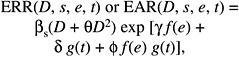
(12B-10)
where e is age at exposure in years and t is time since exposure in years. The functions of age at exposure evaluated were f(e) = e; f(e) = e* = (e − 30) / 10 for e < 30, and 0 for e 0; and the RERF model in which f(e) was an indicator for one of the three categories: e < 20, 20 e < 40, and e 40. The functions of time since exposure evaluated were g(t) = log (t) and g(t) = t. The committee also fitted ERR models for leukemia of the form shown in Equation (12B-10).
Table 12B-6 shows the drop in deviance (compared to a model with no modification by e or t) for both the EAR and the ERR models. For comparisons among different models of the same type (EAR or ERR), the greater the drop in deviance, the better is the fit. Because it is not meaningful to compare the drop in deviance for an EAR model to that for an ERR model, the total deviances are also shown. In general, models in which age at exposure was treated as a continuous variable fitted the data nearly as well even though they have fewer parameters. Comparing the use of e and e* in models that are otherwise the same resulted in very similar fits, with slightly better fits with e*. The use of log (t) resulted in better fits that the use of t.
For the EAR models using e* and log (t) (models 5–7), the interaction term [e* × log (t)] was clearly needed (p < .001), but the main effect for log (t) was not (p > .5). With the main effect for log (t) in the model (model 5), the EAR decreases with time since exposure for those exposed under about age 25, but increases slightly with time since exposure at older exposure ages. Without the main effect (model 7), the EAR remains constant with time since exposure for those exposed over age 30 and decreases with time since exposure for those exposed under age 30, with a stronger decrease at the youngest ages. The latter model is the committee’s preferred EAR model for estimating leukemia risks. With this model, there was no need for an interaction of sex and time since exposure (p = .23), which was included in the UNSCEAR (2000b) leukemia model.
The committee’s preferred ERR leukemia model is model 5. With this model, the ERR decreases with time since exposure regardless of age at exposure, although the decrease is not as strong at older ages. Again, there was no strong evidence of a need for an interaction of sex and time since expo-
TABLE 12B-6 Comparison of Fits of Several Models (as Measured by the Deviance) Expressing the Dependence of Risk of Leukemia Mortality on Age at Exposure (e) and Time Since Exposure (t)a
|
Model Number |
Age at Exposure (e), f(e) |
Time Since Exposure (t) or Attained Age (a), g(t) or g(a) |
Difference in Deviance for This Model and Model with No Modification by e or t (degrees of freedom) |
Deviance |
||
|
EAR Model |
ERR Model |
EAR Model |
ERR Model |
|||
|
1 |
Categoricalb |
log (t): full model |
21.3 (5) |
21.4 (5) |
2254.9 |
2258.7 |
|
2 |
e − 30 |
log (t): full model |
20.1 (3) |
22.5 (3) |
2256.1 |
2257.6 |
|
3 |
e − 30 |
log (t): main effect only ( |
9.4 (2) |
20.2 (2) |
2266.8 |
2259.8 |
|
4 |
e − 30 |
log (t): interaction only (δ = 0) |
19.5 (2) |
13.3 (2) |
2256.7 |
2266.8 |
|
5 |
e*c |
log (t): full model |
21.1 (3) |
24.9 (3) |
2255.1 |
2255.1 |
|
6 |
e* |
log (t): main effect only ( |
9.4 (2) |
21.9 (2) |
2266.9 |
2258.2 |
|
7 |
e* |
log (t): interaction only (δ = 0) |
20.4 (2) |
22.9 (2) |
2255.8 |
2257.2 |
|
8 |
Categorical |
t |
17.7 (5) |
19.9 (5) |
2258.5 |
2260.2 |
|
9 |
e − 30 |
t: full model |
15.9 (3) |
21.0 (3) |
2260.3 |
2259.1 |
|
10 |
e* |
t: full model |
18.2 (3) |
23.9 (3) |
2258.1 |
2256.1 |
|
aBased on analyses of leukemia mortality (1950–2000) using models in which the EAR or ERR is given by βs(d + θd2) exp [γ f(e) + δ g(t) + iconid=pphi f(e) g(t)]. bSeparate estimates for e < 20, 20 e < 40, e 40. ce* is min[(e − 30) / 10, 0], where e is age at exposure in years. |
||||||
sure (p = .15). The total deviances for the preferred EAR and ERR leukemia models were nearly identical.
Thus, the committee’s preferred models for the EAR and the ERR are as follows, with δ = 0 for the EAR model:
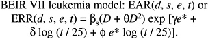
(12B-11)
The parameter estimates for the committee’s preferred leukemia models are listed in Table 12-3 in the main chapter. Figure 12-2 shows both the ERR and the EAR as a function of time since exposure for exposure ages of 10, 20, and 30+ years. The ERR model is similar to that used for all leukemia by NIH (2003), although its leukemia model was based on e instead of e*, and on t instead of log (t), and did not allow for the dependence of the ERR on sex. Although there was no indication that the ERR depended on sex, this was included for compatibility with models for site-specific solid cancers.
ANNEX 12C: DETAILS OF LAR UNCERTAINTY ANALYSIS
Uncertainty Due to Sampling Variability
The approximate variance of the estimated LAR due to the uncertainty in LSS estimated linear models can be derived with the “delta method” (Feinberg 1988). As an example, the estimated LAR based on relative risk transport for solid cancer (for males or females) is calculated as
(12C-1)
where e* = e − 30 if e (exposure age) is less than 30 years and 0 otherwise; B(a) is the age-specific baseline rate at age a for the cancer of interest; S(a) is the probability of survival (in the 1999 U.S. population) to age a; and the Greek letters with hats represent the estimated coefficients in the excess relative risk model. The logarithm of Equation (12C-1) gives
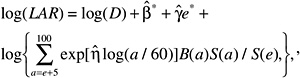
where ![]() .
.
The result of a first-order Taylor’s approximation about ![]() is
is
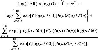
so that the estimate of log (LAR) is a constant plus ![]() , where
, where
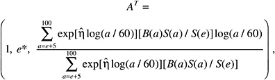
and ![]() . Then var[log(LAR)] may be estimated by
. Then var[log(LAR)] may be estimated by
(12-C2)
where V is the estimated variance-covariance matrix of ![]() , which is available as a component of the output from the computer program used to estimate the risk models. The standard error of the log of estimated LAR is the square root of the estimate of this variance. A 95% confidence interval for log (LAR) is obtained as the estimate of log (LAR) plus and minus 1.96 times the standard error, and the confidence interval for LAR is obtained by taking the antilogarithm of these end points.
, which is available as a component of the output from the computer program used to estimate the risk models. The standard error of the log of estimated LAR is the square root of the estimate of this variance. A 95% confidence interval for log (LAR) is obtained as the estimate of log (LAR) plus and minus 1.96 times the standard error, and the confidence interval for LAR is obtained by taking the antilogarithm of these end points.
The LAR based on absolute risk transport is
The issues and computations involve only slight modifications of what has been described above. For scenarios that involve a weighted average of different ages at exposure and for relative and absolute risk models for leukemia, which involve quadratic-in-dose terms and different modifiers including interactions, the computations differ but the ideas behind the delta method calculations are the same as above.
The confidence intervals in Tables 12-5A and 12-5B for risks of cancer incidence and mortality at specific sites were based on the same procedure as above, but without accounting for the uncertainty in γ and η, since, with a few exceptions, these quantities were fixed at their values estimated from all solid cancers combined (although the values of γ and η used in site-specific models were compatible with data for each site, the fixed values cannot be considered unbiased estimates of the correct values). For most sites, uncertainty in the estimated coefficient of dose (β) is quite large and is expected to dominate the uncertainty in the estimated LAR.
Combining Several Sources of Uncertainty
A single estimate of LAR is obtained from estimates based on ERR and EAR transport models as a combination on the log scale: log (LAR) = [p (log (LARERR) + (1 − p) log (LAREAR)], where LARERR and LAREAR are the estimates based on ERR and EAR transport, respectively, and p is a number between 0 and 1, reflecting the relative strength of belief in the two transport models. For most cancers, a value of .7 was taken for p. Exceptions were lung cancer, where p = .3, and thyroid cancer, where only an ERR model developed from data on Caucasian women was available. A further adjustment to the single estimate of LAR, due to the presumed curvature in the dose-response, is obtained by dividing this combined estimate by the presumed DDREF. A value of 1.5 was used for DDREF, which is an estimate of the median of the Bayesian posterior probability distribution for DDREF, as discussed in the chapter.
The uncertainty analysis here arrives at an approximate variance for log (LAR), emanating from the individual variances in LARERR and LAREAR (sampling variability from the LSS risk model estimation, as discussed above), p (uncertainty in the knowledge of whether absolute risk or excess risk is transportable from Japanese A-bomb survivors to the U.S. population), and DDREF (uncertainty in estimating dose-response curvature from animal studies and uncertainty with which the animal curvature applies to humans).
To accomplish this, the model above is written more formally as depending on four sets of unknown quantities: θR, the parameters in the relevant ERR model; θA, the parameters in the EAR model; IR, an indicator variable that takes on the value 1 if the ERR model is the correct one for transport and 0 if the EAR model is the correct one; and θDDREF, the unknown DDREF. The LAR associated with an acute radiation dose D at age e may be written as
where LARR(e, D; θR) and LARA(e, D; θA) are the LARs based on EAR and ERR transport, prior to DDREF adjustment, and θDDREF is the correct DDREF value. Notice that if the ERR model is the correct one for transport, then IR is 0 and the LAR expression above reduces to LARA(e, D; θA / θDDREF. Similarly, if the relative risk model is the correct one for transport, then the LAR expression reduces to the excess relative risk LAR with DDREF adjustment.
The estimated LAR can be expressed by the same formula, but with the known parameters replaced by their estimators: ![]() , where
, where ![]() and are parameter estimates for the ERR and EAR models;
and are parameter estimates for the ERR and EAR models; ![]() is the (subjective) probability that the relative risk model is the correct one for transport; and
is the (subjective) probability that the relative risk model is the correct one for transport; and ![]() is the (subjective) estimate of DDREF. Every quantity with a “hat” on it is an uncertain estimator and has a variance associated with it. The variance in the estimated LAR, consequently, is that which is propagated by the variances of these estimators.
is the (subjective) estimate of DDREF. Every quantity with a “hat” on it is an uncertain estimator and has a variance associated with it. The variance in the estimated LAR, consequently, is that which is propagated by the variances of these estimators.
Statistically, it is best to consider this propagation on the log scale:

With the simplifying approximation that the “hats” can be dropped from ![]() and
and ![]() in the middle term and the assumption that the uncertainties due to risk model estimation, subjective assessment of DDREF, and subjective as-
in the middle term and the assumption that the uncertainties due to risk model estimation, subjective assessment of DDREF, and subjective as-
sessment of transport model are independent of one another, the variance of the log of the estimated LAR is the sum of three pieces:
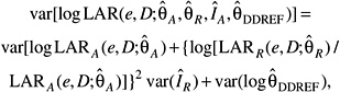
which are due, respectively, to the variability in the parameter estimators in the EAR model, the uncertainty in the transport model, and the uncertainty in the DDREF. It is a fairly simple matter to estimate the variance of the log (LAR) from these quantities. The variance of log (LAR), with a normal approximation to the sampling distribution of log (LAR), leads directly to the coefficient of variation in Table 12-10 and the subjective confidence intervals in Tables 12-6 and 12-7.
The simplifying approximation mentioned above amounts to assuming that ![]() log and log
log and log ![]() have equal variances and a correlation of 1 or, in other words, that the variance of an average of these two quantities is the same as the variance of either one individually. The effect of inaccuracies in this assumption is expected to be small relative to the overall variability. Furthermore, because the first term in the variance expression represents the variance of the estimated LAR for either transport model, a weighted average of
have equal variances and a correlation of 1 or, in other words, that the variance of an average of these two quantities is the same as the variance of either one individually. The effect of inaccuracies in this assumption is expected to be small relative to the overall variability. Furthermore, because the first term in the variance expression represents the variance of the estimated LAR for either transport model, a weighted average of ![]() and
and ![]() is used to estimate it (with the weight corresponding to the strength of belief in the relative risk transport model).
is used to estimate it (with the weight corresponding to the strength of belief in the relative risk transport model).
The approach for estimating the variances of the sampling distributions of the estimated LARs is discussed in the first section of this annex. The variance of ![]() is taken to be Bernoulli variance. If, for example, the probability that the relative risk transport is correct is taken to be .7, then the variance of
is taken to be Bernoulli variance. If, for example, the probability that the relative risk transport is correct is taken to be .7, then the variance of ![]() is .7 × 0.3. The Bernoulli variance tends to be larger than a variance from a uniform distribution (for a model in which the correct transport is some completely unknown combination of relative and absolute risk) or from a beta distribution (for a model in which the correct transport is some unknown combination, but with more specific information about the possible combination). In the absence of any real knowledge about which of these is correct, the committee has elected to use the more conservative approach, which leads to somewhat wider confidence intervals.
is .7 × 0.3. The Bernoulli variance tends to be larger than a variance from a uniform distribution (for a model in which the correct transport is some completely unknown combination of relative and absolute risk) or from a beta distribution (for a model in which the correct transport is some unknown combination, but with more specific information about the possible combination). In the absence of any real knowledge about which of these is correct, the committee has elected to use the more conservative approach, which leads to somewhat wider confidence intervals.
As discussed in Annex 11B, the DDREF analysis is necessarily rough and the variance of the uncertainty distribution described there is, if anything, misleadingly small. For the uncertainty analysis considered here, therefore, the variance representing the uncertainty in log (DDREF) was inflated by 50%, using 0.09 as the variance of ![]() , rather than the derived posterior variance 0.06.
, rather than the derived posterior variance 0.06.
ANNEX 12D: ADDITIONAL EXAMPLES OF LIFETIME RISK ESTIMATES BASED ON BEIR VII PREFERRED MODELS
Tables 12D-1 and 12D-2 show lifetime risk estimates for cancer incidence and mortality resulting from a single dose of 0.1 Gy at several specific ages. Estimates are shown for all cancer, leukemia, all solid cancer, and cancer of several specific sites. Table 12D-3 shows analogous lifetime risk estimates for exposure to 1 mGy per year throughout life and to 10 mGy per year from ages 18 to 65. The examples below illustrate how these tables may be used to obtain estimates for other exposure scenarios. For clarity of presentation, the committee has generally shown more decimal places than are justified.
Example 1: A 10-year-old male receives a dose of 0.01 Gy (10 mGy) to the colon from a computed tomography (CT) scan. Table 12D-1 shows the estimated lifetime risk of being diagnosed with colon cancer for a male exposed to 0.1 Gy at age 10 as 241 per 100,000. The estimate for a male exposed at 0.01 Gy is obtained as (0.01 / 0.1) × 241 = 24.1 per 100,000 (about 1 in 4000). An estimate of the lifetime risk of dying of colon cancer can also be obtained using Table 12D-2, and is (0.01 / 0.1) × 117 = 11.7 per 100,000 (about 1 in 8500).
Example 2: A 45-year-old woman receives a dose of 0.001 Gy (1 mGy) to the breast from a mammogram. Table 12D-1 shows an estimated lifetime risk of being diagnosed with breast cancer for a female exposed to 0.1 Gy at age 40 as 141 per 100,000; the comparable estimate for exposure at age 50 is 70 per 100,000. Using linear interpolation, the risk from exposure to 0.1 Gy at age 45 is (141 + 70) / 2 = 105.5 per 100,000. The risk from exposure to 0.001 Gy is estimated as (0.001 / 0.1) × 105.5 = 1.055 per 100,000. A rough estimate of the risk from repeated annual mammograms could be obtained by adding estimates obtained from receiving a mammogram at ages 45, 46, 47, 48, and so forth. For most purposes, such an estimate will be reasonable, although this approach does not account for the possibility of dying before subsequent doses are received.
Example 3: A female is exposed to high natural background of 0.004 Gy (4 mGy) per year throughout life. Lifetime risk estimates for exposure to 0.001 Gy (1 mGy) per year throughout life are shown in columns 2 (incidence) and 4 (mortality) of Table 12D-3. To obtain estimates for exposure to 4 mGy throughout life, these estimates must be multiplied by 4. For example, the estimated risk of a female being diagnosed with a solid cancer would be 3872 (4 × 968), per 100,000 whereas the risk of being diagnosed with leukemia would be 204 (4 × 51) per 100,000, yielding a total risk of being diagnosed with cancer of 4076 per 100,000 (about 1 in 25). The risk of dying of cancer can be obtained in a similar manner and would be 1988 per 100,000 (about 1 in 50).
TABLE 12D-1 Lifetime Attributable Risk of Cancer Incidencea
TABLE 12D-2 Lifetime Attributable Risk of Cancer Mortalitya
TABLE 12D-3 Lifetime Attributable Risk of Solid Cancer Incidence and Mortalitya


