
Appendix A
Modeling Methods
In Chapter 2, we define models and describe the distinguishing features that could be considered for staffing models for the Federal Aviation Administration’s (FAA) aviation safety inspectors (ASIs). We note that predictive, stochastic models, designed as decision support tools, that assist with both allocation and sufficiency decisions, are most appropriate for the FAA’s staffing models. We briefly note the distinction between process models and statistical models and conclude that a process-modeling approach may be superior in the FAA’s context because it is more easily adapted during environmental changes of the type that characterize today’s aviation landscape. The purpose of this appendix is to more precisely describe those two approaches, to emphasize the crucial role that parameter estimation plays in either modeling approach, and to note that statistical procedures are often used to estimate the parameters in process models.
Process Modeling
Process models take many forms, from simple flowcharting to more complex discrete-event simulation. In this discussion, we focus on discrete-event simulation as a more robust form of process modeling that permits prediction of complex system behavior as a result of system design. In this case, the system to which we refer is the FAA regulatory and oversight system that employs ASIs to ensure aviation safety. System design includes all of the factors that drive staffing demand as well as the supply and work capacity of ASI inspectors. In this discussion, we as-
sume that one wants to determine through the use of process models how the two are interrelated, so that reasonable inferences can be drawn regarding the relationship between staffing system design and staffing system performance.
The specific approach we use to illustrate process modeling is known as task network modeling. In a task network model, system functions (e.g., performing all the required inspections in a region) are decomposed into a series of subfunctions, which are then decomposed into tasks. This is, in engineering terms, a task analysis. The sequence of tasks is defined by constructing a task network .
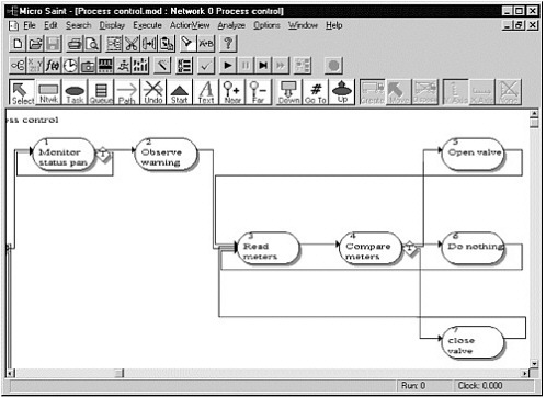
This concept is illustrated in Figure A-1, which shows a sample task network for a simple procedure—responding to a warning indication. The appropriate level of system decomposition and the portion of the system that is simulated depend on the particular problem. Staffing models have been developed that examine human behavior at the molecular level (e.g., detailed individual user interaction with the human-computer interface) and at a much more aggregated level (e.g., at which the task-level behaviors take hours or days).
In the ASI staffing context, the model might be at a gross level of granularity, since it need only represent inspectors or groups of inspectors as “busy” or “available.” The details of what they are doing are important only to the extent that they relate to factors that drive work demand and capacity.
The task network must also represent in some way the dynamics and dependencies of each task. Such factors include time to perform each task (possibly means and standard deviations), conditions that must be met for the task to start (e.g., available inspector resources, completion of a prerequisite task), and how performance of a given task interacts with other parts of the system.
Every time more than one path out of a task is defined in the network, a decision must be made by a human or other system element on what potential course of action should be followed, and the decision rules must be included in the model. The branching probabilities or decision logic can be represented by numbers, equations, algorithms, and logic of any complexity. In an ASI staffing model, the decision rules would reflect such factors as ASI task prioritization (e.g., required, planned, or demand work).
The paragraphs above describe the essential information that must be defined to adequately represent the relationships underlying a complex process such as the ASI staffing system. However, before a model can be useful in making predictions, it must be capable of accepting and processing changes in its inputs. In particular, the model must be able to accept and process a changing set of demands on the system (e.g., changing the
number, location, and mix of carriers, aircraft, and other elements that generate demand for ASI services) as well as a changing supply of ASIs (e.g., changing the number, type, and location of ASI inspectors in the part of the ASI system being modeled). When the staffing model is capable of accepting and processing changes to inputs, decision makers can use the model to estimate resulting changes in outputs. Those outputs can be as varied as the systems they represent. Typical outputs for staffing process models fall into two general categories: measures of personnel utilization (e.g., how busy will each type of ASI be at each location?) and estimates of delays in work completion associated with the unavailability of staff to perform the work. Such outputs allow users to estimate the effectiveness with which ASI staffing resources are used and their ability to meet work demand. There are many ways to express and quantify such information, and a model can be designed to provide the most appropriate and usable output to serve the needs of its users.
Statistical Modeling
A statistical model is based on observed empirical relationships—in this instance, the relationship between workload and the staffing necessary to accomplish the workload. The relationships are specified initially in mathematical form; the parameters or coefficients of the model are then estimated statistically from the data. Repeated observations that pair the workload accomplished with the staff hours expended to accomplish the workload are the minimum data necessary. Other variables should be added if they affect the relationship between workload and staffing; these might include location-specific factors. For example, some locations may require far more staff hours to accomplish a set of inspections when those inspections require extensive travel time by the ASI; in this case, a location factor that accounted for the relatively lower productivity of ASIs in certain locations would need to be included in the model.
An advantage of this statistical (or empirical) approach is that it does not require a detailed understanding of the process by which the work is accomplished. It does require, however, an understanding of the factors that may differentially affect productivity across work centers, so that the effects of these factors can be captured in the relationship. The process model approach breaks down the work tasks to the fundamental elements and models those elements. The statistical approach, in general, models the aggregate relationship. Under the statistical approach, one does not require an understanding of the detailed steps to estimate the aggregate relationship and apply those estimates in a staffing model.1
Methods used in estimating relationships in the model include ordinary least squares regression, nonlinear least squares regression, and maximum likelihood methods. The relationship in its most general form is given by:
where y is staffing, measured in hours, days, or full-time equivalents (FTE), and the Xs are workload and factors affecting the staffing-workload relationship. A multivariate model, in which all important observable factors affecting productivity are captured, will provide the best estimates of prediction.
If the functional form or mathematical relationship specified were linear, then the model would be of the form:
where the parameters (α, β) are estimated from the data using, for example, ordinary least squares regression.
Because the statistical model uses the empirically observed relationship between staffing and workload, actual productivity is embedded in the model. The estimated relationship is usually based on the average observed productivity. It is also possible to estimate a “frontier” production function that provides the maximum (rather than the average) workload that can be accomplished (see, for example, Greene, 2002).
A major limitation of the statistical approach is that when processes or productivity changes, the previously observed statistical relationship is no longer valid. New data, generated under the new conditions, must be used to re-estimate the relationship. Thus, if it is known that the existing relationships between staffing and workload are not the relationships that will govern future staffing, then a process model approach would be more appropriate. With a process model approach, when a process changes, the model must also be modified to reflect the change. The difference is that, for a process model, the new process may be simulated, perhaps based on analysis and expert judgment, without waiting for new data to be generated.
Finally, it is important to recognize that the dichotomy drawn here between a process simulation model and a statistical model may be overstated. A process model may use statistical methods to estimate some or all of its parameters, while a statistical model may include relationships between workload or intermediate output at fine levels of detail, similar to the tasks and steps of the process model.
Parameter Estimation
Regardless of the type of model—process simulation, statistical model, or another type of model—values must be obtained for the key parameters of the model. These parameters provide the relationship between input variables or factors and intermediate or final output.
In the statistical model, by its nature, the key parameters are estimated statistically using actual data from observations or records of the key relationships. Hence, the parameter estimates are objective and empirically based. Moreover, the standard error of the parameter estimates can be calculated, using standard statistical methods. This provides an estimate of the accuracy of the parameter estimates.2
In the process model, there will also be parameters that must be estimated. In general, because a process model attempts to capture all or most of the key steps or processes in the staffing-workload relationship, there are likely to be more parameters to be estimated than in the statistical model.
Methods of estimating the parameters may include the same statistical methods as the statistical models themselves. That is, if the process model requires an estimate of the time required to make a certain type of inspection, one way to estimate this is through statistical estimation using data on actual inspection times, perhaps including other factors affecting the inspection time.
A second way to estimate parameters is through calibration. If one has data on the outcomes and basic inputs, one can calibrate the model by running it with a set of parameters specified using judgment. The model’s outcomes are compared with actual outcomes, and the parameters adjusted in directions anticipated to improve the fit or agreement between the simulated outcome and the actual outcome. The process is repeated until a satisfactory set of parameters—one that yields a satisfactory fit—is obtained. The calibration process is similar to statistical estimation, but less formal. Because of its informal nature, the properties of the parameter estimates are not formally established. However, it does have the advantage of being empirically based.
Finally, expert judgment can serve as the basis for determining key
relationships between staffing and workload or intermediate steps in the process. While expert judgment can be useful, it must ultimately be validated by the accuracy of the predictions that are made with the model using the judgment-based parameters. Because expert judgment is subjective, it risks rapid loss of credibility without such validation.


