Procedures and Standards for a Multipurpose Cadastre (1983)

A base map is the graphic representation at a specified scale of selected fundamental map information; used as a framework upon which additional data of a specialized nature may be compiled (American Society of Photogrammetry, 1980). Within the multipurpose cadastre, the base map provides a primary medium by which the locations of cadastral parcels can be related to the geodetic reference framework; to major natural and man-made features such as bodies of water. roads, buildings, and fences; and to municipal and political boundaries. The base map also provides the means by which all land-related information may be related graphically to cadastral parcels.

Good planning and engineering practice dictate the preparation of large-scale maps as a basis for sound community development and redevelopment. In urban areas. and particularly in growing urban areas, such large-scale maps are currently being compiled at an unprecedented rate by photogrammetric methods. Relatively simple changes in the specifications governing these photogrammetric mapping opcrations can make the resulting maps not only more effective planning and engineering tools but can, at relatively little additional cost, lay the foundation for the eventual creation of a multipurpose cadastre.

There are three fundamental forms that may be used to represent map information: (1) line map. (2) photographic or orthophotographic map, and (3) digital map. The conventional line map is a line and symbol representation of natural and selected

man-made features on a coordinate reference system. Different line, symbol, and area colors are used to aid in distinguishing between water features. man-made objects, wooded areas, and contours, A line map is produced from scribed, inked, or pasted-on line copy. A photographic map is a photograph or assembly of photographs on which descriptive cartographic data, marginal information, and a coordinate reterence system have been overprinted. The photographs may be uncontrolled, nominally vertical aerial photographs, or they may be rectified photographs, with image displacements due to camera tilt removed. An orthophotographic map is similar to a photographic map with the exception that, in generating the orthophotographs from conventional aerial photographs, image displacements caused by both camera tilt and terrain relief are removed. Photographic images on an orthophotographic map are therefore in their correct orthographic map position. Digital maps have evolved in recent years with the development of powerful data-processing systems that have made it possible to collect and store digitized map data. Manipulation and merging of the digitized data and selective retrieval of desired levels of map information, either in graphic form as a plot or a printout or in numerical form as a body of data, make the digitized representation of map information (virtual map) a very flexible form (Thompson, 1979).

Each of the forms of map information (line map, photographic map, and digital map) has its advantages and disadvantages as candidates for a base-mapping medium in a multipurpose cadastre. The majority of map-producing organizations today are producing line maps. To a considerable extent, a line map can selectively control the type and amount of information to be shown on the base map. However, line maps are the most difficult and expensive to update in a timely fashion. Photographic maps can be readily updated with the collection and processing of new photography, and they contain a large amount of terrain surface detail. As a base map, however, the photographic map may have more detail than desired, without the possibility for control of the type and amount of information to be shown. Image displacements in the photographic map due to camera tilt and terrain relief are removed in the orthophotographic map, with the additional expense of the differential rectification process necessary to produce the orthophotograph. With the development of the techniques of automated cartography, digital mapping promises to be the form most responsive to the requirements for flexible selection of type and amount of base-map information and for regular base-map updating. Only in this form can map information that has been collected at different scales and in different formats be efficiently merged, digitally, and displayed together. Necessary digital mapping standards will evolve as this new technology matures in future production mapping environments. Their development is being advanced currently by a Committee on Digital Cartographic Data Standards organized in 1982 by the American Congress on Surveying and Mapping, with the sponsorship of the U.S. Geological Survey (Mocllering, 1982).

There are three alternatives to be considered when evaluating the source materials to be used for base maps in a multipurpose cadastre: (1) existing maps (line, photographic, or digital), (2) existing maps updated with new map information during the course of the cadastre operation, and (3) new maps. The tradeoffs among the alternatives are map uniformity and accuracy versus the cost of new mapping.

Unless there has been a consolidation and standardization of the mapping effort within the various departments to a single, unified mapping activity, and a recent large-scale mapping program completed, existing maps for a given county or municipality are likely to be incomplete, out of date, or otherwise less than ideal for use as a mapping base for the cadastral overlay. The basic mapping functions in a typical local government environment, at the county level for example, are generally spread among a number of departments or divisions, primarily (1) assessment, (2) public works, and (3) planning. The base-map requirements for each of these departments vary, especially with regard to map scale, format, and content. This situation fosters a general lack of coordination among departments, duplication of effort, and often an absence of adequate, professional mapping personnel (Archer, 1980). The accuracy of the existing maps may be unknown or not adequate for present-day urban requirements. The cost of immediate new mapping, on the other hand, may appear to be prohibitive. Thus the need to consider the alternatives.

Substantial savings can be realized by adapting a new map system to existing base maps, if they are adequate. For example, in Prince William County, Virginia, a new Mapping Division was created as a consolidation of the mapping efforts of the Finance and Assessments Division, the Public Works Department, and the Planning Office. The division developed a unified mapping program using 1:2400-scale base maps, with 320 maps covering the 345 square miles of the county. Prior to consolidation, the property identification maps alone numbered 597. These maps originally included 197 at a scale of 1:4800 and 400 at a scale of 1:1200. In preparation for the 1:2400 base-map scale, the property identification maps are being photomechanically reduced or enlarged and then digitized so that computer plotted overlays can be drawn at the base-map scale and any other scale desired. A cost analysis of the Prince William County system indicates that $158,000 was being expended annually, prior to consolidation of the mapping program, to maintain the separate mapping efforts. With an anticipated increase in the number of larger-scale property identification maps, this $158,000 was expected to increase to $178,000. It was estimated that complete coverage of the county at the 1:2400 base-map scale would cost $350,000, which reduces to about $1000 per square mile. However, since the Public Works Department’s topographic maps at the 1:2400 scale were found to be of high quality, cost of completion of the base mapping was only $150,000, or $435 per square mile. With the significantly reduced number of maps, the annual maintenance cost for the unified mapping program is $75,000, less than half of the cost before program consolidation (Archer, 1980).

The state of Missouri is taking the approach of a new, statewide comprehensive mapping program. The State Tax Commission supported a study in late 1979 by GRW Consulting Engineers, Inc., of Lexington, Kentucky, to assist in the design and development of a new statewide base-mapping program. The state has a land area of approximately 69,000 square miles, with 2,300,000 land parcels administered in 115 assessment jurisdictions. Recommendations for mapping bases included photographic maps using aerial photographs, orthophotographic maps, and planimetric line maps. Rectified photographic maps would be used at 1:2400 and 1:4800 scales where relief was not excessive. Orthophotographic maps would be used at 1:2400 and 1:4800 scales where topography was excessive and for all maps at a 1:1200 scale. The planimetric line map would be used where 1:600-scale base maps are required. Of the 115 assessment jurisdictions, 109 counties covering an area of 66,437 square miles required the full mapping program. The six jurisdictions excluded were those in the Kansas City and St. Louis areas, containing over half of the state population.

The base-map needs and costs projected in 1980 by the consulting engineers for

this new statewide program appear in Table 3.1. In the initial stages of this program, which are just recently under way. orthophotography is being used as the standard base-map system, at a cost that is ranging between $250 and $500 per square mile.

Design of the base-mapping data content and structure must be flexible enough to allow a variety of users to relate the cadastral parcels to specific types of base information. This objective can readily be achieved by creating and maintaining the base-mapping data in a coordinated series of different levels or overlays. Photographic and orthophotographic base maps at a minimum contain the complete photographic image of the terrain surface covered. to which other levels or overlays may be added to create the complete base map.

The primary base-map datum is the geodetic reference framework used to cstablish the location of all other features. The following reference systems are in current use throughout the United States:

1. Geographic Coordinates (latitude and longitude)

2. Universal Transverse Mercator (UTM) rectangular coordinates

3. State Plane Coordinates

Geographic coordinates provide the principal system used for computation of geodetic control-point positions. The UTM rectangular coordinate system is a metric worldwide system of predominate use in federal mapping environments. State Plane Coordinates are most commonly used at the state and local levels, currently defined in English units but with metric units also widely available with completion of the National Geodetic Survey readjustment of the North American Horizontal Datum in 1983. Because of the greater familiarity with their use at the local level, State Plane Coordinates are normally used as the geodetic reference framework in current implementation projects and are recommended for local multipurpose cadastres (see Section 2.2.2).

Natural and cultural features that are relatable to a cadastral parcel form the next most important levels of base-map data. One of these levels includes all streets, roads, railroads, and airports, with their associated names. Another level includes all permanent buildings and other structures greater than a specified size. A third level includes all water features such as perennial and intermittent streams, natural and man-made lakes and ponds, reservoirs, canals, and aqueducts and their associated names. A fourth level includes boundaries of civil (governmental) jurisdictions at all levels: state, county, city, and township. Other secondary levels of natural and cultural features, such as contours. floodplains, wetlands, vegetation cover, land use, and utility lines, may be included selectively in the base-map composite.

Use of a number of different levels or overlays of base-map data is essential to provide flexibility in meeting the different requirements of different map users. Drafted overlays must be precisely registered in position to each other as illustrated in Figure 3.1 (Archer, 1980). A planner may desire, for example, to use as a working base a composite of the land-use, floodplain, and base-map overlays. The greatest flexibility in base-map content, to satisfy user requirements, is in digital mapping. Map information can be separated digitally into a maximum number of data levels, updated most efficiently, and plotted precisely on a single base sheet using any specified number of data levels as required. At the same time, standards and procedures must yet be established to control the level of map content detail as map scale is changed over wide ranges.

Overall, the base map that supports a multipurpose cadastre must provide as a minimum enough planimetric detail for locating ownership boundaries referenced to natural features, such as stream and lake shorelines, or to man-made features not as yet tied to the coordinate system, such as highways and railroads. Desirably, it should

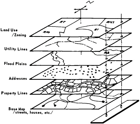
FIGURE 3.1 A registered overlay system.

show all objects related to the location of real-property boundaries, such as fences or driveways, at reasonably frequent intervals.

Accuracy of the horizontal and vertical position information on the base map is fundamentally a function of the map scale and contour interval, respectively. National Map Accuracy Standards (Appendix B) have long been used as the primary standard to control the accuracy of plotted map information. For scales larger than 1:20,000, which include essentially all base maps that would be used to support a cadastral overlay, standards for horizontal accuracy specify that 90 percent of the points tested shall be plotted on the map within 1/30 inch of their true position. Standards for vertical accuracy specify that 90 percent of the points tested shall be shown in elevation within one half of the contour interval used on the map.

The Photogrammetry for Highways Committee of the American Society of Photogrammetry has prepared specifications for large-scale mapping for highways, with a horizontal accuracy requirement that 90 percent of all planimetric features be plotted within 1/40 inch of their true position (U.S. Department of Transportation, 1968). This is a more stringent requirement than the comparable 1/30 inch required by National Map Accuracy Standards and has also been suggested by the Task Committee for Photogrammetric Standards of the American Society of Photogrammetry in their recently proposed Accuracy Specifications for Large Scale Line Maps. Either the 1/30-inch or 1/40-inch requirements have been adopted by nearly all users in their base-mapping specifications for large-scale property-ownership maps.

The requirement that the base map of a local record system be compiled according to National Map Accuracy Standards (Appendix B) is primarily due to the need for the base map to satisfy the engineering needs of public works departments. When accurate information is necessary, specific boundary lengths would come from a recorded plat, boundary description, or other report of survey, not from scaling the cadastral overlay on the base map. A new Engineering Map Accuracy Standard has been proposed by the Committee on Cartographic Surveying of the Surveying and Mapping Division of the American Society of Civil Engineers (ASCE). These standards are intended to provide a clearer communication of accuracy requirements between those having the need for the map and those preparing the map. Also included are specific field-testing procedures to assess the compliance of the map with the standards.

Whatever standard is agreed on, the need exists for quality control within a basemapping program to verify conformance of the mapping to standards. An accuracycheck ground survey is necessary to determine the ground positions of checkpoints for comparison with their corresponding mapped position. Evaluation of the checkpoint results, using the National Map Accuracy Standard, can be accomplished by

first computing the standard error, σ=[Σ,x_i²/(n − 1)] ¹². where x₁, x₂,…x_n are the errors observed at the n checkpoints. Assuming a normal distribution for the checkpoint errors, the 90 percent error can then be computed as 1.645σ and then compared with the accuracy standard. Care must be taken to ensure that the map position of checkpoints has not been deliberately altered to accommodate standard map symbolization. The proposed ASCE Engineering Map Accuracy Standards specify the use of 20 well-defined and widely distributed points for determination of the checkpoint discrepancies. At least 15 percent of the checkpoints shall appear in each quadrant of the map. The accuracy-check ground survey shall be at least of an order of accuracy equal to that of the control survey on which the map is compiled. This proposed standard would not identify specific error values (such as 1/30 inch or one-half contour interval as cited in the National Map Accuracy Standards) but rather leaves those values for negotiation between the engineering client and the cartographic engineer. Evaluation of the accuracy-check ground survey is made by computing limiting standard errors in each of the X, Y, and Z positions, for comparison with the values specified during negotiation, and also computing limiting mean absolute errors in each of the X, Y, and Z positions, again for comparison with the values specified (American Society of Civil Engineers, in preparation).

The scale of the cadastral map system is principally a function of the size of the predominant land parcel. This criterion generally corresponds to the level of land value or degree of urbanization. Listed in Table 3.2 are the scales that have been selected almost universally for each type of area. In the Missouri Tax Mapping Project, for example, the scale of the base maps varied with lot frontage, indicated in the second column in this table.

Contours may only need to be included on the base map for specific users with a requirement for topographic detail. The added expense is substantial. Contour interval would be selected in conjunction with the map scale, the terrain relief, and the elevation information requirements. Typical combinations are listed in Table 3.3.

Typical mapping cameras with nominal 6-inch focal-length lenses are flown at altitudes below 25,000 ft above mean terrain for the collection of aerial photography. With the increasing usefulness of orthophotographic maps. interest has grown in high-altitude photography using cameras with focal lengths of 6, 12, 24, and 36 inches. The higher the altitude, with the same focal-length camera, the smaller the relief displacement that must be corrected in the photograph for a given amount of terrain relief on the ground. Availability of modified commercial jet aircraft with pressurized cabins has increased the operational flight altitude to 50,000 ft above mean sea level.

Since 1978, the U.S. Geological Survey (USGS) has been developing a National High-Altitude Photography program consisting of both black-and-white panchromatic and color infrared 9-inch×9-inch photographs taken at a flight altitude of 40.000 ft above mean sea level. The black-and-white photographs are taken with an aerial camera with a focal length of 6 inches, resulting in a photo scale of 1:80,000, each frame representing nearly 130 square miles on the ground. The color infrared photographs are taken by a camera with a focal length of 8.25 inches, resulting in a photo scale of 1:58,000, each frame covering nearly 68 square miles. Standard enlargements are 2×, 3×, and 4×. With flight lines running in a north-south direction, the black-and-whitc camera exposes a photograph over the center of each USGS 7 1/2-minute mapping quadrangle. The color infrared photographs are particularly useful in resource inventories, agricultural monitoring, and pollution detection.

The NASA U-2 aircraft, based at the NASA Ames Research Center, have a maximum operating altitude of from 65,000 to 70,000 ft above mean sea level. The ground resolution of U-2 imagery collected at 65,000 ft above mean terrain

varies from 0.1 to 20 m (0.3 to 65 ft) as shown in the tabulation of camera configurations in Table 3.4 (National Aeronautics and Space Administration, 1978). While being used primarily in water-resource and land-use management studies, and in providing ground-truth support for satellite imagery investigations (e.g., Landsat), high-altitude photography has definite potential as a data source for base-map information both as a photograph map and in digital form. Two NASA U-2 aircraft are available on a cost-reimbursable basis for collection of high-altitude photography. Over one third of the United States already has U-2 photographic coverage available, with primary concentrations of coverage over the eastern and western regions of the country.

With the launching in July 1972 of the Earth Resources Technology Satellite (ERTS1), later renamed Landsat 1, concentration by NASA on gathering information from the Earth’s surface began, nearly 15 years after Sputnik 1 in 1957. The success that Landsat has enjoyed is generally attributed to its long life and its repeated coverage of the same regions, rather than to its ability to produce images of high resolution. Landsat 1 was followed by Landsat 2 in 1975 and Landsat 3 in 1978. The technical characteristics of these satellite systems, and others, are presented in Table 3.5 (American Society of Photogrammetry, 1980). The low resolution of Landsat— 1:1,000,000 and 1:500,000 scales with 79- and 40-m-square ground-resolution picture elements or “pixels” (that is, about 260 or 130 ft square)—precludes the recording of small cultural features. The positional accuracy of well-defined points on a multispectral scanner (MSS) frame has been reported by Colvocoresses (1975) to be as good as 50 m (164 ft). Landsat images have typically been enlarged by some users by four times, to a scale of 1:250,000. The USGS has compiled and printed blackand-white and color image maps from Landsat frames, at scales ranging from 1:250,000 to 1:1,000,000. Map and chart revision has been accomplished successfully on selected features such as bodies of water, vegetation, and bold cultural objects with scales in some cases as large as 1:50,000. A study in Prince Georges County, Maryland, used the Landsat image to determine the area of various census tracts. Table 3.6 has the comparison of the Landsat results with the Metropolitan Council of Governments’ (COG) values. While the direct application of Landsat imagery to support cadastral base mapping is limited, Landsat data can be interpreted to differentiate among a broad variety of surface features. This information can be put to practical use in such applications as agricultural crop forecasting, rangeland and forest management, mineral and petroleum exploration, land-use management. water-quality evaluation, and disaster assessment. Map information from these applications can ultimately be merged with the cadastral base map and overlay to relate the information to the land parcel. Use of Landsat imagery is important because of the large volume of frames available and the continuance of the project with Landsat D. While future

satellite systems are scheduled to carry sensors with a reported 10-m ground resolution, only after the resulting materials have been evaluated will their increased usefulness to cadastral base mapping be known.

The advantages resulting from the collection, storage, and manipulation of base-map information in digital form have been presented earlier. The flexibility of being able to assemble a composite map of different levels of digital map data. and update and extract those levels in a timely manner as new information becomes available. is only possible with an interactive graphics system working with the map information in digital form.

Digital data acquisition may be from previously existing maps, from new mapping. from photogrammetric stercomodels, from ground surveys. or from other terrain information data sources. The usual method of data collection from maps is by manually following the map feature lines on a digitizer table, a tedious operation with a high probability of errors, caused by either duplicating or omitting information. Automatic line-following instruments, usually with the assistance of an operator, improve the accuracy of the data collection. A second approach to automatic data acquisition from maps is to use a scanning device with either a single-element detector or a linear array. Working with the separate overlays (levels) of the map information, this procedure requires a significant amount of computer time to identify and connect together the individual segments of lines in the required “vector” format.

Direct digitizing from photogrammetric stereomodels is facilitated by the use of linear or rotary encoders on the axes of the photogrammetric plotting instruments. Either stereomodel coordinates or photographic image coordinates are recorded in-

itially, with computer program processing transforming the positions into the ground reference coordinate system. The direct link between the stereocompiler and the digital storage eliminates the usual intermediate manuscript preparation stage and subsequent digitizing from the manuscript. This methodology yields a reduction in human intervention and results in ultimately higher accuracies on the digital map (Delaware Valley Regional Planning Commission, 1980). Elevation data can be formatted either as contour lines, profiles with elevations recorded at regular intervals or at breaks in terrain slope, or as geomorphic points along drainage lines or hillcrests, for example. Some photogrammetric instruments are equipped with automatic image correlators that produce a high density of elevation data points.

Each level of map information is stored in its own “layer,” in conjunction with other like elements, in the manner depicted in Figure 3.1. This allows for retrieval of any desired combination of levels, such as roads and contours or buildings and property lines. The layering also provides the greater flexibility in producing maps and in an easier update process.

It is essential that the cadastral parcel layer of a digital map system contain complete topological references. That is, each property-line segment in the cadastral overlay must have its own unique identifier and a record that includes the identifiers of its end points as well as the parcels that it bounds. Each end point of propertyline segments also must have a unique identifier and a record identifying the line segments and the parcels that meet there. Attached to these point and line records should be other information on their locations. the date and accuracy of the location measurements, and how the points can be relocated in the field. Only with such complete topological and survey data can a digital cadastral overlay be a “living map” that is readily updated as conditions change and that submits readily to automated tests for its completeness and consistency. The same is true for any other overlay intended to be a complete and up-to-date public record, e.g., of a utility system.

The initial interactive graphics task is usually data editing. While data editing may be done by producing a graphic plot on a digitally controlled plotting table, the typical procedure would be to display the data on a digitally controlled cathode-ray tube (CRT). The operator can then determine overlapping, erroneous, or missing data and either make the corrections on the CRT or request a redigitization of the manuscript or stereomodel.

Raw digital data are rarely in form for immediate use, and extensive computer preprocessing is typically required to arrange the data in an appropriate format. This preprocessing may include coordinate transformation from stereomodel coordinates to the ground reference system such as Universal Transverse Mercator Coordinates or State Plane Coordinates. Most data-acquisition schemes acquire far more data than are actually required in the final data files. Therefore, techniques of data compression must be employed to reduce the amount of data to a manageable quantity. Another requirement of the preprocessing system is format conversion, to convert

elevation data, for example, interchangeably between contours, profiles, and regular grids of recorded elevation.

Storage of the enormous amounts of digital map data requires an organized system for retrieval. For most modern systems, magnetic tape is the basic storage medium. Header information on each tape will identify the map area, the type of information, and the format in which it is recorded. If digital map data are to be transferable from one facility to another, format standards must be established and used. One such standard has been prepared for data exchange between graphic data bases (American Public Works Administration Research Foundation, 1979b).

Digital map data are being collected in increasingly massive volumes. The Defense Mapping Agency has digitized the contour data on the 1:250,000-scale maps of the entire United States. These data have been turned over to the USGS for storage maintenance and dissemination to users. The USGS has a long-range objective of producing a digital cartographic data base that will contain essentially all of the information now shown on the existing 1:24,000-scale topographic quadrangle maps, both elevation information and planimetric data. This data base will initially contain 11 types of base-map data as follows:

1. Reference Systems—geographic and other coordinate systems except the Public Land Survey System.

2. Hypsography—contours, elevations, and slopes.

3. Hydrography—streams and rivers, lakes and ponds, wetlands, reservoirs. and shorelines.

4. Surface Cover—woodland, orchards, and vineyards.

5. Nonvegetative Features—lava rock, playas, dunes, slide rock, and barren waste areas.

6. Boundaries—political jurisdictions, national parks and forests, and military reservations.

7. Transportation Systems—roads, railroads, trails, canals, pipelines, transmission lines. bridges, and tunnels.

8. Other Significant Man-Made Structures—buildings, airports, and dams.

9. Geodetic Control, Survey Monuments, Landmark Structures.

10. Geographic Names.

11. Orthophotographic Imagery.

Other national mapping organizations in Canada, Great Britain, and Australia are also producing digital cartographic data bases.

Within the private sector, digital data bases are being collected in a number of industries, notably those in petroleum, mining, timber, and public utilities. Four companies with extensive digital data bases across the United States are Phillips Petroleum Company, Tobin Research, Inc., Petroleum Information, Inc., and Stratigraphic Services Company. Much of the data base collected includes digitized section

corners of the Public Land Survey System. The digital maps created are exploration maps and lease and ownership maps. These vary in scales from 1:24,000 to 1:1200.

The interactive graphics system is the working tool for digital data storage and manipulation. The hardware and software elements work together in the following functions:

1. Creation of a digital map data base including textual, numeric, and graphic information on geographic facilities and statistical data;

2. Editing of a digital map data base;

3. Selective retrieval of various subsets of data from the data base for presentation on graphic displays and alphanumeric displays and for making digital maps;

4. Producing data tapes in a standard interchange format containing selected subsets of the digital data base;

5. Producing reports from various subsets of data in tabular form.

A procurement specification for an interactive graphics system has been prepared under the Computer Assisted Mapping and Records Activity System (CAMRAS) program by the American Public Works Administration Research Foundation (1979a).

Implementation of the digital-mapping capabilities described above has expanded enormously over the past 10 years, with hundreds of systems currently in place. The

typical system consists of a mainframe minicomputer, disk and magnetic tape units, station interface hardware, graphics software. graphics work stations, and a plotter. Other optional peripherals such as line printers, hard-copy units, alphanumeric terminals, and on-line stereoplotters may also be a part of the system. Acquisition of the interactive graphics capability may occur in one of a number of ways, from the complete development of the entire hardware/software components to the purchase of a “turnkey” hardware/software system to the purchase of the capability as a service. The advantages and disadvantages of the possible approaches are presented in Table 3.7 (Dangermond and Smith, 1980).