
1
Projected World Energy Consumption
HARRY PERRY and HANS H. LANDSBERG
Resources for the Future, Inc.
1.1
INTRODUCTION
Basic to any evaluation of the potential impact of man’s use of energy resources on climate are estimates of how much energy will be consumed at various locations, which resources, and how much of each will be used to supply the demand, how much will be converted to other energy forms before use, and what pollutants and how much of each will be emitted as a result of use of the projected mix of fuel forms.
Climatic effects from energy consumption may occur as the result of either heat that is released (over that incident upon the earth from the sun) or the effect that pollutants may have on both the amount of solar energy that reaches the earth and the amount that is radiated from the earth to space.
In the following sections, energy consumption and pollution emissions are estimated for eleven geographic regions and for four different years, the last year being 2025. Section 1.2 presents best estimates of energy resources for the world and for component parts, separately for nonrenewable and renewable sources, paying particular attention to the recoverability factor, i.e., how much of the resource in place can be mobilized for use. Section 1.3 presents estimates of energy demand, based upon projections of population and Gross National Product (GNP). A detailed exposition of the merits precedes the estimates. Section 1.4 gives estimates of the heat, carbon dioxide, and particulates that can be expected to be released by energy use.
1.2
WORLD ENERGY SUPPLIES
NONRENEWABLE WORLD ENERGY RESOURCES
Table 1.1 lists the currently used nonrenewable world energy resources by fuel form and by two categories of resource availability. The “proved recoverable” category is the quantity of each resource whose existence is known with some relatively high degree of precision and that can be produced using currently available extraction technologies at current costs. The “estimated total remaining recoverable” category is that quantity of each fuel that is thought to be included in the earth’s crust, will be discovered, and will be recover-
TABLE 1.1 World Developed Nonrenewable Energy Resources, 1972a
|
|
Proved Recoverable, Btu × 1018 (J × 1021) |
Estimated Total Remaining Recoverable, Btu × 1018 (J × 1021) |
||
|
Coal |
24.0 |
(25.3) |
168.0 |
(177.2) |
|
Crude oil and natural gas liquids |
3.5 |
(3.7) |
12.0 |
(12.7) |
|
Natural gas |
2.0 |
(2.1) |
11.0 |
(11.6) |
|
Oil shale and tar sands |
2.0 |
(2.1) |
15.8c |
(16.7) |
|
U3O8b |
1.3 |
(1.4) |
2.5 |
(2.6) |
|
|
32.8 |
(34.6) |
209.3 |
(220.8) |
|
aSources: World Energy Conference, Survey of Energy Resource, 1974; World Power Conference, Survey of Energy Resources, 1965; H. R. Linden and J. D. Parent, “Analysis of World Energy Supplies,” Survey of Energy Resources, 1974; Senate Committee on Interior and Insular Affairs, U.S. Energy Resources: A Review As Of 1972, Part I, Committee Print 93–40 (92–75) (U.S. Govt. Printing Office, Washington, D.C., 1974); Oil and Gas J., Dec. 31, 1973, p. 86. bAssuming 1.5 percent efficiency use of the U3O8 and cost cutoff level of $10 and $15 per pound of U3O8 for “proved” and “remaining,” respectively. For characterization of these highly restrictive assumptions, see text. cAssuming use of oil shale containing 15 or more gallons/ton (51.5 liters per metric too or more) this number would exceed 50 × 1018 Btu (52.8 × 10²¹ J). The 15.8 × 10¹⁸ was derived by using the lowest value for oil shale and tar sands as reported in the WEC. |
||||
able using current or new technology that might be developed and at prices that may prevail in the future. The category includes four types of resource: proved resources; those that have been discovered and cannot now be produced at current prices with current technology but could be with improved technology or higher prices; those that would now be commercially producible but have not yet been found; and those that, if found now, would not be commercially producible with present technology at present prices but would be expected to be recoverable in the future with new technology and at future prices.
The accuracy of information even about “proved and currently recoverable resources” is quite variable since the precision of these estimates is different for each country. As a result, a variety of values for “proved recoverable” resources can be found in published literature for the various fuel forms. The spread in the published values for the “estimated total remaining recoverable” category is usually much wider, since such estimates involve a much higher degree of judgment about what new resources will be found, what new technologies will be developed, and what the future prices of the various energy resources will be.
The basic sources used in preparing Table 1.1 were World Energy Conference (WEC), Survey of Energy Resources, 1974; World Power Conference, Survey of Energy Resources, 1965; H. R. Linden and J. D. Parent, “Analysis of World Energy Supplies,” Survey of Energy Resources, 1974 (World Energy Conference, 1974); Senate Committee on Interior and Insular Affairs, U.S. Energy Resources, A Review As Of 1972, Part I, Committee Print 93–40 (92–75), 1974; and Oil and Gas Journal, December 31, 1973, p. 86.
Table 1.1 indicates the “best” estimate* for each category and for each fuel. The “best” values to be used for tar sands and oil shale are very uncertain. If all the estimated oil shale resources containing 51.5 liters or more per metric ton (15 gallons per ton) were included, the values in Table 1 would be much larger than the 15.8 × 10¹⁸ Btu (16.67 × 10²¹ J) actually shown.
In a recently published report of the National Academy of Sciences,† the total remaining recoverable resources of crude oil, natural gas, and coal were estimated at 10 × 1018, 7.2 × 10¹⁸, and 264 × 1018 Btu (10.55 × 10²¹, 7.60 × 10²¹, and 278.52 × 10²¹ J). The crude oil estimates are 16 percent lower and the natural gas estimates are nearly 34 percent lower than those in this paper. However, the coal estimates are about 57 percent higher than those shown in Table 1.1. Considering the great uncertainties involved in these kinds of estimates the agreement between this report and the unpublished data is considered to be very good for oil and gas and good for coal.
The uranium estimates are highly conservative and possibly misleading on two grounds. First, they do not take into account the possible development of the breeder reactor. The efficiency of light-water reactors assumed in the tabulation is about one fortieth of that of the breeder. Thus, in terms of energy, the estimated uranium resources would be 40 times as large if used in a breeder reactor. Second, the convention for considering both reserves and what is called here “remaining recoverable resources” of uranium has been to set up limiting cost levels. These have for a long time been $8 per pound of U3O8 and have only in the last few years been raised to $15 (always in current dollars), with estimates up to $30 first established in 1975. Nothing comparable is available for most foreign countries. In the context of rapidly rising prices of competing fuels and the declining sensitivity of power costs to the price of uranium (given the rapid escalation of plant cost), uranium above—and perhaps far above the $15 cutoff—will qualify as “economic.” This would be especially true for the breeder in which the relative importance of fuel costs is very small. For these reasons the figures here shown, which are limited to $15 material, are highly conservative and subject to change. During 1975, purchases in the United States were indeed made at prices as high as $40, though these should not be taken as establishing a new price floor. Lifting the “no breeder” constraint alone would raise the level several tens of times. Raising the $15 constraint to, for example, $30 would at least double the amount. Raising it to $100, which is not an unreasonable proposition, could raise it by a factor of 10 or 20.
Figure 1.1 is a plot of the estimated depletion rates of
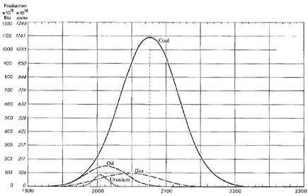
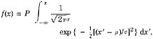
FIGURE 1.1 Idealized depletion curve for the world’s (less the United States) coal, oil, gas, and uranium resources, 1900–2300. The general equation for the depletion curves is
![]()
where the constants are
coal P = 1096.5 × 1015, μ = 2076, σ = 42;
oil P = 146.25 × 10¹⁵, µ = 2012, σ = 30;
gas P = 99.25 × 10¹⁵, µ = 2046, σ = 40;
uranium P = 60 × 1015, µ = 2005, σ = 12.
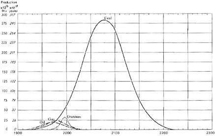
FIGURE 1.2 Idealized depletion curve for U.S. coal, oil, gas, and uranium resources, 1900–2300. The general equation for the depletion curves is
![]()
where the constants are
coal P = 284.5 × 10 15, μ = 2078, σ = 45;
oil P = 19.5 × 10¹⁵, μ = 1972, σ = 22;
gas P = 24 × 1015, μ = 1979, σ = 19;
uranium P = 31 × 1015, μ = 1996, σ = 9.
world developed nonrenewable energy resources* (excluding the United States) by each type of resource using idealized depletion curves. If the breeder reactor or fusion is commercially available by 2000 to 2010, then supplies of energy will present no problem for the world in the period to 2025 and well beyond. The possible shortfall (see below) of world energy supplies that could occur by 2025 if only nonrenewable resources, hydroelectricity, and light-water reactors are used would have to be filled by geothermal resources, wind power, and solar energy. Should these energy resources not be developed by that time in the quantities needed, the depletion rates of the nonrenewable resources would have to be accelerated over that shown in the idealized depletion curves, and the bell-shaped curves shown in Figure 1.1 would be compressed toward an earlier total depletion date.
The approximate shape of the curves for each of the resources would actually be determined by the total demand for heat units for the world for each of the future years. This, in turn, can be estimated from regional world population and world GNP in those years. (See Section 1.3.) With a knowledge of total demand, total resource availability, and the general shape that the depletion curve for nonrenewable resources takes, a share of the total demand can be allocated to each resource.
Figure 1.1 does not include U.S. resources or their rate of depletion. This is shown in Figure 1.2. As drawn, these figures treat the rest of the world and the United States as acting independently of each other as far as energy resource production and use are concerned. In fact, if there is free access by the United States to world oil and gas resources,
TABLE 1.2 World Developed Nonrenewable Energy Resources, by Region (Recovery Factor Included)
|
|
Coal, Btu × 1018 (J × 1021) |
Oil, Btu × 1018 (J × 1021) |
Gas, Btu × 1018 (J × 1021) |
Oil Shale and Tar Sands, Btu × 1018 (J × 1021) |
U3O8, Btu × 1018 (J × 1021) |
|
North America (excluding United States) |
1.2 |
0.24 |
0.42 |
2.0 |
0.5 |
|
|
(1.3) |
(0.25) |
(0.44) |
(2.1) |
(0.5) |
|
Western Europe |
5.3 |
0.08 |
0.28 |
0.4 |
0.5 |
|
|
(5.6) |
(0.08) |
(0.30) |
(0.4) |
(0.5) |
|
Oceania |
4.2 |
0.03 |
0.04 |
0.9 |
0.3 |
|
|
(4.4) |
(0.03) |
(0.04) |
(0.9) |
(0.3) |
|
Latin America |
0.6 |
1.07 |
1.07 |
1.9 |
Neg. |
|
|
(0.6) |
(1.13) |
(1.13) |
(2.0) |
Neg. |
|
Asia (excluding Communist) |
|
|
|
|
|
|
Japan |
Neg. |
Neg. |
Neg. |
Neg. |
Neg. |
|
|
Neg. |
Neg. |
Neg. |
Neg. |
Neg. |
|
Other Asia |
2.1 |
3.72 |
4.11 |
2.5 |
Neg. |
|
|
(2.2) |
(3.93) |
(4.34) |
(2.6) |
Neg. |
|
Africa |
1.0 |
1.16 |
1.16 |
3.3 |
0.5 |
|
|
(1.1) |
(1.22) |
(1.22) |
(3.5) |
(0.5) |
|
U.S.S.R. and Communist Eastern Europe |
|
|
|
|
|
|
U.S.S.R. |
61.0 |
3.54 |
2.86 |
0.5 |
— |
|
|
(63.3) |
(3.74) |
(3.02) |
(0.5) |
— |
|
Communist E. Europe |
0.6 |
0.01 |
Neg. |
Neg. |
— |
|
|
(0.6) |
(0.01) |
(Neg.) |
(Neg.) |
— |
|
Communist Asia |
60.0 |
1.15 |
0.06 |
2.5 |
— |
|
|
(63.3) |
(1.21) |
(0.06) |
(2.6) |
|
|
World (excluding United States) |
136.0 |
11.0 |
10.0 |
14.0 |
1.8 |
|
|
(143.5)b |
(11.61)b |
(10.55) |
(14.8)b |
(1.9)b |
|
United States |
32.1 |
1.1 |
1.1 |
1.8 |
0.7 |
|
|
(33.9) |
(1.16) |
(1.16) |
(1.9) |
(0.7) |
|
TOTAL WORLD |
168.1 |
12.1 |
11.1 |
15.8 |
2.5 |
|
|
(177.4)b |
(12.77)b |
(11.71)b |
(16.7)b |
(2.6)b |
|
aAt $15 per pound of U3O8. bConverted figures (in parentheses) may not add because of round-off error. |
|||||
then depletion of these two resources in the rest of the world would occur more rapidly.
Curves similar to those reproduced in Figure 1.1 (for the rest of the world in total) and in Figure 1.2 (for the United States) were prepared for each fuel for each region based on the data in Table 1.2 in order to estimate production by individual fuel and geographic area in future years.*
RENEWABLE ENERGY RESOURCES
There are at least five potentially important renewable energy resources: hydroelectric, geothermal, tidal, solar, and fusion energy. Of these energy forms, hydroelectric is by far the most widely used, solar and geothermal are used to a small extent, tidal applications are minuscule and almost certain to remain so, and the feasibility of fusion technology has yet to be proven. Table 1.3 shows the developed and undeveloped hydroelectric energy resources of the United States and the rest of the world in megawatts of potential capacity. Figure 1.3 shows the estimated amount of worldwide (less the United States) hydroelectric energy that could be available at various future times using what are believed to be reasonable estimates for the rate at which new hydroelectric capacity could be installed.
Figure 1.4 gives a similar projection for the United States. Even if all the potential hydroelectric sites were developed and operated at the assumed conditions, only about 1 per-
TABLE 1.3 Potential World Water-Power Capacitya
|
Region |
Potential, 103 MW (109 Btu/h) |
Percentage of Total, % |
Development, 103 MW (109 Btu/h) |
Percentage Developed, % |
||
|
North America |
313 |
(1068) |
11 |
59 |
(201) |
19 |
|
South America |
577 |
(1969) |
20 |
5 |
(17) |
|
|
Western Europe |
158 |
(539) |
6 |
47 |
(160) |
30 |
|
Africa |
780 |
(2662) |
27 |
2 |
(7) |
|
|
Middle East |
21 |
(72) |
1 |
— |
|
|
|
Southeast Asia |
455 |
(1553) |
16 |
2 |
(7) |
|
|
Far East |
42 |
(143) |
1 |
19 |
(65) |
|
|
Australasia |
45 |
(154) |
2 |
2 |
(7) |
|
|
U.S.S.R., China and Satellites |
466 |
(1590) |
16 |
16 |
(55) |
3 |
|
TOTAL |
2857 |
(9751)b |
100 |
152 |
(519) |
|
|
aSource: Energy Resources, A Report to the Committee on Natural Resources of the National Academy of Sciences-National Research Council (NAS-NRC, Washington, D.C., 1962), p. 99, Table 3. bConverted figures (in parentheses) may not add because of round-off error. |
||||||
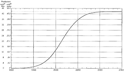
FIGURE 1.3 World (excluding the United States) hydroelectric production potential, 1900–2150. The equation for the production potential is
where P = 41.7 × 10¹⁵, μ = 2015, and σ = 33.
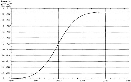
FIGURE 1.4 U.S. hydroelectric production potential, 1900–2150. The equation for the production potential is
where P = 2.275 × 10¹⁵, μ = 1998, and σ = 33.
cent of the energy consumed in the United States and about 3 percent of that of the world would be provided from this renewable resource by the year 2000.
In the analysis that follows, the use of geothermal and solar energy has been assumed to remain small even to the year 2025 in order to test whether there would be sufficient nonrenewable resources to supply demand and to estimate the maximum amount of pollutants that could be released. In fact, small amounts of geothermal energy are being and will be used in the future, and by 2025 solar energy could be making a major contribution to energy supply.
FUTURE AVAILABILITY OF NONRENEWABLE AND HYDROELECTRIC FUEL SUPPLIES BY REGION
From the idealized depletion curves for each of the nonrenewable fuels, estimates of fuel production were made for each region in 1980, 1985, 2000, and 2025. Estimates of hydroelectric production for the different areas of the world for these same years were also made.
The sum of the production rates for each fuel form for all the geographic areas (for 1980, 1985, 2000, and 2025) is not the same as the estimates that are obtained when all the energy resources for each fuel form for the world (less the United States) are first aggregated (Figure 1.1) and then depletion estimates made for each fuel. Although not shown in the accompanying tables for 1980 and 1985, the total estimate made on an aggregated resource basis is less than results from summing the individual depletion estimates for each of the geographic areas. However, although the total is smaller when using the aggregate world values for some individual fuels, the aggregate estimate is larger for uranium and coal and smaller for oil and gas. For the years 2000 and 2025, the production rates that are estimated using the aggregate method of determining resource production (shown in Table 1.4 as “World excluding
TABLE 1.4 Energy Resource Production by Regions, 2025
|
Regions |
Coal, Btu × 1015 (J × 1018) |
Oil, Btu × 1015 (J × 1018) |
Gas, Btu × 1015 (J × 1018) |
Hydroelectricity, Btu × 1015 (J × 1018) |
Uranium, Btu × 1015 (J × 1018) |
Total, Btu × 1015 (J × 1018) |
|
North America excluding United States |
1.9 |
0.9 |
0.2 |
2.4 |
8.0 |
13.4 |
|
|
(2.0) |
(0.9) |
(0.2) |
(2.5) |
(8.4) |
(14.1) |
|
Western Europe |
34.5 |
0.2 |
0.0 |
2.4 |
0.5 |
37.6 |
|
|
(36.4) |
(0.2) |
(0.0) |
(2.5) |
(0.5) |
(39.7) |
|
Oceania |
9.2 |
0.0 |
0.9 |
0.6 |
3.1 |
13.8 |
|
|
(9.7) |
(0.0) |
(0.9) |
(0.6) |
(3.3) |
(14.6) |
|
Latin America |
2.2 |
6.5 |
16.5 |
5.8 |
— |
31.0 |
|
|
(2.3) |
(6.9) |
(17.4) |
(6.1) |
|
(32.7) |
|
Japan |
— |
— |
— |
— |
— |
— |
|
Other Asia |
22.8 |
21.3 |
51.0 |
6.7 |
— |
101.8 |
|
|
(24.1) |
(22.5) |
(53.8) |
(7.1) |
— |
(107.4) |
|
Africa |
16.6 |
9.4 |
7.1 |
6.0 |
4.5 |
63.6 |
|
|
(17.5) |
(9.9) |
(28.6) |
(6.3) |
(4.7) |
(67.1) |
|
U.S.S.R. |
93.1 |
45.9 |
25.1 |
5.9 |
170.0 |
|
|
|
(98.2) |
(48.4) |
(26.5) |
(6.2) |
|
(179.4) |
|
Communist East Europe |
5.4 |
0.8 |
— |
6.2 |
||
|
|
(5.7) |
(0.8) |
|
|
|
(6.5) |
|
Communist Asia |
60.6 |
20.9 |
— |
81.5 |
||
|
|
(63.9) |
(22.0) |
|
|
|
(86.0) |
|
World (excluding United States) |
246.3 |
105.9 |
120.8 |
29.8 |
16.1 |
518.9 |
|
(259.8) |
(111.7)c |
(127.4) |
(31.4)c |
(17.0)c |
(547.4)c |
|
|
United States |
141.8 |
1.1 |
1.3 |
1.8 |
0.1 |
146.1 |
|
|
(149.8) |
(1.2) |
(1.4) |
(1.9) |
(0.1) |
(154.1) |
|
Total Nonrenewable |
388.1 |
107.0 |
122.1 |
31.6 |
16.2 |
665.0 |
|
|
(409.4)c |
(112.9)c |
(128.8) |
(33.3)c |
(17.1)c |
(701.6) |
|
TOTAL RENEWABLE |
|
|
|
|
|
508.0 |
|
TOTAL ALL ENERGY |
|
|
|
|
|
1,173.0 |
|
|
|
|
|
|
|
(1,237.6) |
|
aTotals included with U.S.S.R. bFigures unavailable. cConverted figures may not add because of round-off error. |
||||||
United States”) are greater than those obtained by surveying the estimated production of the different regions, largely because of differences that arise from the regional and aggregate estimates of coal production in those years. This difference occurs because estimates of the regional production rates for coal were made on the basis of optimizing coal use for each geographic area’s need, while the aggregate estimates optimized coal use for the total world energy requirements.
1.3
ENERGY DEMAND
INTRODUCTION
Worldwide energy demand has grown at an exponential rate during the entire period in which reasonably reliable world energy statistics have been collected. Energy consumed in selected years in the different regions and the percentage shares of these regions are shown in Table 1.5. World energy consumption over the period 1925 to 1968 had an average growth rate of about 3.5 percent per year, but the rate has been increasing. Between 1925 and 1938, the rate was less than 2 percent per year; between 1960 and 1965 it was 5½ percent per year.
Growth rates, however, have varied widely among the different regions, as shown by the shifting percentages of the total used by the various regions in the values given in the bottom half of Table 1.5. From 1925 to 1972, the U.S. share of the total decreased from 48.3 percent to 32.8 percent; that of Western Europe from 34.8 percent in 1925 to only 19.6 percent in 1968. On the other hand, the U.S.S.R. increased its share from 1.7 to 15.7 percent of the total in this period. The less developed areas too increased their percentage share, indicating a growth rate in energy demand that exceeded that of North America and Western Europe. However, these regions still consume only a small portion of the world’s energy, since their growth in energy use has been from a small (starting) base
TABLE 1.5 Energy Consumption, by Major World Regions, Selected Years, 1925–1971a,b
|
Region |
1925 |
1938 |
1950 |
1955 |
1960 |
1965 |
1967 |
1968 |
1971 |
|
Million Metric Tons |
|
|
|
|
|
|
|
|
|
|
North America of which: United States |
748.9 |
706.9 |
1276.3 |
1461.3 |
1659.5 |
2040.2 |
2230 |
2359 |
2529 |
|
717.7 |
669.4 |
1201.0 |
1370.3 |
1550.1 |
1881.6 |
2055 |
2173 |
2327 |
|
|
Western Europe |
517.0 |
619.2 |
583.9 |
748.2 |
849.5 |
1117.2 |
1168 |
1242 |
1388 |
|
Oceania |
15.6 |
18.1 |
29.3 |
37.3 |
45.8 |
61.2 |
67 |
72 |
80 |
|
U.S.S.R and Communist E. Europe |
80.5 |
244.0 |
464.1 |
691.2 |
934.5 |
1255.8 |
1376 |
1433 |
1591 |
|
U.S.S.R. |
25.3 |
176.3 |
303.3 |
461.0 |
640.6 |
880.6 |
989 |
1025 |
1112 |
|
Communist E. Europec |
55.1 |
67.7 |
160.8 |
230.2 |
293.9 |
375.1 |
387 |
408 |
479 |
|
Communist Asiac |
23.7 |
27.3 |
43.1 |
98.3 |
235.3 |
323.0 |
255 |
332 |
477 |
|
Latin America |
24.7 |
38.7 |
66.2 |
105.4 |
153.5 |
199.5 |
224 |
245 |
274 |
|
Asiad |
60.3 |
112.4 |
105.8 |
157.7 |
247.7 |
385.1 |
471 |
522 |
635 |
|
Japan |
30.5 |
62.4 |
45.8 |
66.5 |
111.0 |
188.6 |
249 |
280 |
342 |
|
Other Asia |
29.8 |
50.0 |
60.0 |
91.2 |
136.7 |
196.5 |
222 |
242 |
293 |
|
Africa |
13.9 |
23.4 |
42.0 |
58.8 |
70.2 |
92.6 |
97 |
102 |
121 |
|
WORLD |
1484.5 |
1790.1 |
2610.9 |
3358.2 |
4196.1 |
5474.6 |
5888 |
6306 |
7095 |
|
Percentage Distribution, % |
|
|
|
|
|
|
|
|
|
|
North America of which: United States |
50.4 |
39.5 |
48.9 |
43.5 |
39.5 |
37.3 |
37.9 |
37.4 |
35.6 |
|
48.3 |
37.4 |
46.0 |
40.8 |
36.9 |
34.4 |
34.9 |
34.5 |
32.8 |
|
|
Western Europe |
34.8 |
34.6 |
22.4 |
22.3 |
20.2 |
20.4 |
19.8 |
19.7 |
19.6 |
|
Oceania |
1.1 |
1.0 |
1.1 |
1.1 |
1.1 |
1.1 |
1.1 |
1.1 |
1.1 |
|
U.S.S.R. and Communist E. Europe |
5.4 |
13.6 |
17.8 |
20.6 |
22.3 |
22.9 |
23.4 |
22.7 |
22.4 |
|
U.S.S.R. |
1.7 |
9.8 |
11.6 |
13.7 |
15.3 |
16.1 |
16.8 |
16.3 |
15.7 |
|
Communist E. Europec |
3.7 |
3.8 |
6.2 |
6.9 |
7.0 |
6.9 |
6.6 |
6.5 |
6.8 |
|
Communist Asiac |
1.6 |
1.5 |
1.7 |
2.9 |
5.6 |
5.9 |
4.3 |
5.3 |
6.7 |
|
Latin America |
1.7 |
2.2 |
2.5 |
3.1 |
3.7 |
3.6 |
3.8 |
3.9 |
3.9 |
|
Asiad |
4.1 |
6.3 |
4.1 |
4.7 |
5.9 |
7.0 |
8.0 |
8.3 |
8.9 |
|
Japan |
2.1 |
3.5 |
1.8 |
2.0 |
2.6 |
3.4 |
4.2 |
4.4 |
4.8 |
|
Other Asia |
2.0 |
2.8 |
2.3 |
2.7 |
3.3 |
3.6 |
3.8 |
3.8 |
4.1 |
|
Africa |
0.9 |
1.3 |
1.6 |
1.8 |
1.7 |
1.7 |
1.6 |
1.6 |
1.7 |
|
WORLD |
100.0 |
100.0 |
100.0 |
100.0 |
100.0 |
100.0 |
100.0 |
100.0 |
100.0 |
|
aAll figures based on coal equivalents. bSources: Data for 1925–1968 from J. Darmstadter, with P. D. Teitelbaum and J. G. Polach, Energy in the World Economy: A Statistical Review of Trends in Output, Trade, and Consumption Since 1925 (Johns Hopkins U. Press, Baltimore, Md., 1972), p. 10; data for 1971 from United Nations. World Energy Supplies, Series J. No. 16 (UN. New York, 1973). cIt should be borne in mind that throughout this study pre-World War II data for “Communist Eastern Europe” refer to the present countries of that area with the exception of prewar East Germany, which appears (as part of Germany) within Western Europe. Prewar “Communist Asia” refers to Mainland China, while the postwar figures for that region also include North Korea, Mongolia, and (beginning in 1955) North Vietnam. dThroughout this study, unless otherwise specified, “Asia” means non-Communist Asia. |
|||||||||
ENERGY CONSUMPTION AND GROSS NATIONAL PRODUCT
A relatively good (but far from perfect) correlation has been shown to exist between energy consumption and GNP. A typical plot of this relationship is shown in Figure 1.5, in which energy consumption per capita for the 49 countries is plotted against the GNP per capita. The plotted points, using 1965 data, fall within a narrow band of the line representing the best fit of all the data with a correlation coefficient of 0.87. If the hydroelectric data used in this plot are corrected to take into account the fossil fuel inputs that would be required to produce this energy (increasing the energy consumption from this resource by a factor of about 3), the correlation coefficient is increased to 0.89.
The reasons that per capita energy consumption and GNP are highly correlated are in general quite obvious, but they are not well enough understood when it comes to changes in the relationship over time or differences between countries. For example, it is hard to explain persuasively why in the United States a steady (but not constant) decline in energy consumption per unit of GNP was sharply reversed in the latter part of the 1960’s. It has also not been possible to disaggregate energy use by consuming sectors in sufficient detail to explain the marked differences in energy use per unit of GNP between the United States and Western Europe or the changes in energy use per unit of GNP that occur over time in nearly all countries. For example, it is not understood why the United States used 2.75 kg of coal equivalent (2.75 × 10⁻³ metric ton of coal equivalent) per dollar of GNP in 1965, while France used only 1.57 kg (1.57 × 10⁻³ metric ton); or why the amount of energy used per unit of GNP produced in Spain rose from 0.67 during 1960– 1965 to 1.48 in 1965–1971.
In spite of the difficulty in explaining in detail the empirical relationship that has been found to exist, its persistence over time and the high correlation coefficient between the two variables suggest that it is useful for projecting world
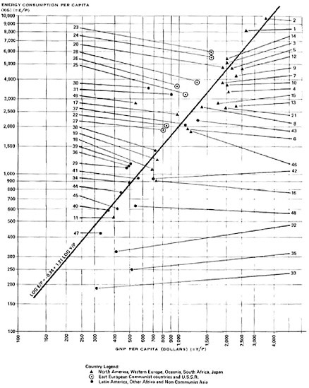
FIGURE 1.5 GNP per capita and energy consumption per capita: 49 selected countries, 1965 (see Table 1.6). Source: J. Darmstadter, with P. D. Teitelbaum and J. G. Polach, Energy in the World Economy: A Statistical Review of Trends in Output, Trade, and Consumption Since 1925 (Johns Hopkins U. Press, Baltimore, Md., 1972), pp. 66–67.
TABLE 1.6 GNP per Capita and Energy Consumption per Capita (see Figure 1.5)
|
|
|
|
|
|
|
Energy Consumption |
|||
|
|
|
(GNP per Capita) ($74) GNP per Capita ($65) |
Per Capita |
Per $1 of GNP (In 1974 $) |
|||||
|
|
Number on Chart |
kg of Coal Equiv. |
|
kg of Coal Equiv. |
|
||||
|
Country |
Dollars |
|
Rank |
Rank |
Rank |
||||
|
North America |
|
|
|
|
|
|
|
|
|
|
Canada |
1 |
2,658 |
(4,079) |
2 |
8,077 |
2 |
3.04 |
(1.98) |
7 |
|
United States |
2 |
3,515 |
(5,394) |
1 |
9,671 |
1 |
2.75 |
(1.79) |
10 |
|
Western Europe |
|
|
|
|
|
|
|
|
|
|
Belgium-Luxembourg |
3 |
1,991 |
(3,055) |
10 |
5,152 |
6 |
2.59 |
(1.69) |
12 |
|
France |
4 |
2,104 |
(3,228) |
7 |
3,309 |
16 |
1.57 |
(1.02) |
37 |
|
West Germany |
5 |
2,195 |
(3,368) |
6 |
4,625 |
8 |
2.11 |
(1.38) |
20 |
|
Italy |
6 |
1,254 |
(1,924) |
20 |
1,940 |
28 |
1.55 |
(1.01) |
38 |
|
Netherlands |
7 |
1,839 |
(2,822) |
13 |
3,749 |
12 |
2.04 |
(1.33) |
22 |
|
Austria |
8 |
1,365 |
(2,095) |
17 |
2,584 |
23 |
1.89 |
(1.23) |
24 |
|
Denmark |
9 |
2,333 |
(3,580) |
4 |
4,149 |
10 |
1.78 |
(1.16) |
27 |
|
Norway |
10 |
2,015 |
(3,092) |
8 |
3,621 |
13 |
1.80 |
(1.17) |
26 |
|
Portugal |
11 |
396 |
(608) |
46 |
520 |
45 |
1.31 |
(0.85) |
42 |
|
Sweden |
12 |
2,495 |
(3,828) |
3 |
4,604 |
9 |
1.85 |
(1.21) |
25 |
|
Switzerland |
13 |
2,331 |
(3,577) |
5 |
2,699 |
21 |
1.16 |
(0.76) |
45 |
|
United Kingdom |
14 |
1,992 |
(3,057) |
9 |
5,307 |
5 |
2.66 |
(1.73) |
11 |
|
Finland |
15 |
1,750 |
(2,685) |
14 |
2,825 |
19 |
1.61 |
(1.05) |
33 |
|
Greece |
16 |
772 |
(1,185) |
29 |
904 |
39 |
1.17 |
(0.76) |
44 |
|
Ireland |
17 |
981 |
(1,505) |
24 |
2,359 |
24 |
2.41 |
(1.57) |
16 |
|
Spain |
18 |
686 |
(1,053) |
33 |
1,080 |
36 |
1.57 |
(1.02) |
35 |
|
Yugoslavia |
19 |
743 |
(1,140) |
30 |
1,217 |
32 |
1.65 |
(1.08) |
32 |
|
Oceania |
|
|
|
|
|
|
|
|
|
|
Australia |
20 |
1,910 |
(2,931) |
12 |
4,697 |
7 |
2.46 |
(1.60) |
13 |
|
New Zealand |
21 |
1,970 |
(3,023) |
11 |
2,603 |
22 |
1.32 |
(0.86) |
40 |
|
U.S.S.R. and Communist E. Europe |
|
|
|
|
|
|
|
|
|
|
Bulgaria |
22 |
829 |
(1,272) |
27 |
2,011 |
27 |
2.43 |
(1.58) |
15 |
|
Czechoslovakia |
23 |
1,561 |
(2,395) |
16 |
5,870 |
3 |
3.76 |
(2.45) |
3 |
|
East Germany |
24 |
1,562 |
(2,397) |
15 |
5,534 |
4 |
3.54 |
(2.31) |
6 |
|
Hungary |
25 |
1,094 |
(1,679) |
22 |
3,188 |
18 |
2.91 |
(1.90) |
8 |
|
Poland |
26 |
980 |
(1,504) |
25 |
3,552 |
14 |
3.62 |
(2.36) |
5 |
|
Romania |
27 |
778 |
(1,194) |
28 |
1,916 |
30 |
2.46 |
(1.60) |
14 |
|
U.S.S.R. |
28 |
1,340 |
(2,056) |
18 |
3,819 |
11 |
2.85 |
(1.86) |
9 |
|
Latin America |
|
|
|
|
|
|
|
|
|
|
Mexico |
29 |
475 |
(729) |
42 |
1,104 |
35 |
2.33 |
(1.52) |
17 |
|
Trinidad and Tobago |
30 |
646 |
(991) |
34 |
3,505 |
15 |
5.43 |
(3.54) |
1 |
|
Venezuela |
31 |
882 |
(1,353) |
26 |
3,246 |
17 |
3.68 |
(2.40) |
4 |
|
Costa Rica |
32 |
414 |
(638) |
45 |
317 |
47 |
0.77 |
(0.50) |
48 |
|
Guatemala |
33 |
318 |
(488) |
49 |
188 |
49 |
0.59 |
(0.38) |
47 |
|
Jamaica |
34 |
492 |
(755) |
41 |
873 |
40 |
1.77 |
(1.15) |
28 |
|
Nicaragua |
35 |
527 |
(809) |
38 |
247 |
48 |
0.70 |
(0.46) |
49 |
|
Panama |
36 |
495 |
(760) |
40 |
1,112 |
34 |
2.25 |
(1.47) |
19 |
|
Puerto Rico |
37 |
1,094 |
(1,679) |
23 |
2,126 |
26 |
1.94 |
(1.26) |
23 |
|
Argentina |
38 |
718 |
(1,102) |
31 |
1,471 |
31 |
2.05 |
(1.34) |
21 |
|
Chile |
39 |
497 |
(763) |
39 |
1,119 |
33 |
2.25 |
(1.47) |
18 |
|
Peru |
40 |
367 |
(563) |
47 |
577 |
44 |
1.57 |
(1.03) |
36 |
|
Uruguay |
41 |
573 |
(879) |
35 |
958 |
37 |
1.67 |
(1.09) |
31 |
|
Asia |
|
|
|
|
|
|
|
|
|
|
Cyprus |
42 |
702 |
(1,077) |
32 |
927 |
38 |
1.32 |
(0.86) |
41 |
|
Israel |
43 |
1,325 |
(2,033) |
19 |
2,248 |
25 |
1.70 |
(1.11) |
30 |
|
Lebanon |
44 |
438 |
(672) |
43 |
770 |
41 |
1.76 |
(1.15) |
29 |
|
Hong Kong |
45 |
421 |
(646) |
44 |
605 |
43 |
1.44 |
(0.94) |
39 |
|
Japan |
46 |
1,222 |
(1,875) |
21 |
1,926 |
29 |
1.58 |
(1.03) |
34 |
|
Malaysia and Singaporea |
47 |
332 |
(509) |
48 |
424 |
46 |
1.28 |
(0.83) |
43 |
|
Africa |
|
|
|
|
|
|
|
|
|
|
Libya |
48 |
542 |
(832) |
36 |
613 |
42 |
1.13 |
(0.74) |
46 |
|
South Africa |
49 |
535 |
(821) |
37 |
2,761 |
20 |
5.16 |
(3.36) |
2 |
|
aIncluding Sabah and Sarawak. |
|||||||||
energy use in the future. Therefore, energy consumption estimates for the world and for selected regions have been based on population and GNP projections for the world and individual areas.
HISTORICAL CORRELATION OF ENERGY CONSUMPTION AND GNP
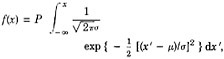
Energy consumption per capita and GNP per capita were correlated for each of the regions listed in Table 1.5 by using data for each region for selected years. A typical plot is shown in Figure 1.6, where the energy consumption per capita and GNP per capita for Japan for selected years from 1925 to 1972 are plotted. The slope of the line indicates how much energy is used for the particular region (or country) per unit of GNP produced. Slopes less than ½ indicate that energy consumption growth rates are lower than GNP growth rates. This is true for the highly industrialized areas such as the United States, Western Europe, and Oceania. The balance of North America, Oceania, Japan, Eastern Europe, and Africa have slopes approximately equal to ½, while Latin America, Other Asia, U.S.S.R., and Communist Asia have slopes much steeper than ½. Except for the U.S.S.R., which has a high energy consumption per unit of GNP that probably results from a planned economy dedicated to a rapid energy-intensive industrialization, the other areas with a high slope are the less developed areas with very low GNP. (Not nearly enough work has been done to rationalize this situation, and it is just possible that the most important element is the substitution of statistically recorded commercial for nonrecorded, noncommercial energy.)
Within each of the areas (or countries) there was a high
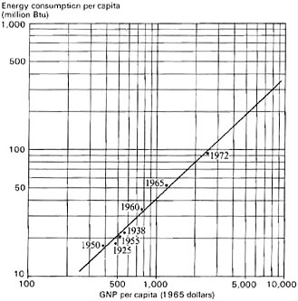
FIGURE 1.6 GNP per capita and energy consumption per capita: Japan. log (E/P) = −1.3178 + 0.9777 log (Y/P).
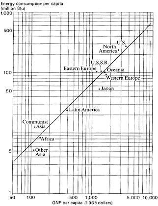
FIGURE 1.7 GNP per capita and energy consumption per capita: 1965. log(E/P) = −1.2023 + 1.0118 log (Y/P).
correlation coefficient for the data for the years that were used. Unfortunately, energy consumption and GNP information over long periods are not always available. Data for the United States, other North America, U.S.S.R., and Japan were obtainable for the period 1925–1972, while data for most of the other areas covered the period 1950–1972.
CROSS-SECTIONAL CORRELATION OF ENERGY CONSUMPTION AND GNP
Energy consumption per capita and GNP per capita were correlated for related years by plotting these data for each of the regions (where available) for given years. A typical plot is shown in Figure 1.7, reflecting the data for 1965 for the 11 regions for which individual energy consumption data have been tabulated. Similar tabulations were made for 1925 (four data points), 1938 (four data points), 1950, 1955, 1960, and 1965 (eleven data points), and 1972 (seven data points).*
It was observed that the slope of the line that best fitted the data became less steep over time, indicating that for the world as a whole energy use per unit of GNP has been de-
TABLE 1.7 Energy Consumption by Regions for the Years 1980, 1985, 2000, and 2025a
|
Region |
1980 Btu × 1015 (J × 1018) |
1985 Btu × 1015 (J × 1018) |
2000 Btu × 1015 (J × 1018) |
2025 Btu × 1015 (J × 1018) |
|
United Statesb |
73 |
84 |
117 |
196 |
|
|
(77) |
(89) |
(123) |
(207) |
|
North America (less U.S.)b |
7 |
8 |
12 |
19 |
|
(7) |
(8) |
(13) |
(20) |
|
|
Western Europeb |
48 |
54 |
81 |
123 |
|
|
(51) |
(57) |
(85) |
(130) |
|
Oceaniab |
3 |
4 |
7 |
15 |
|
|
(3) |
(4) |
(7) |
(16) |
|
Latin Americac |
12 |
16 |
39 |
114 |
|
|
(13) |
(17) |
(41) |
(120) |
|
Japanb |
15 |
19 |
31 |
68 |
|
|
(16) |
(20) |
(33) |
(72) |
|
Other Asiac |
17 |
22 |
55 |
165 |
|
|
(18) |
(23) |
(58) |
(174) |
|
Africac |
5 |
7 |
19 |
78 |
|
|
(5) |
(7) |
(20) |
(82) |
|
U.S.S.R.b |
43 |
56 |
97 |
244 |
|
|
(45) |
(59) |
(102) |
(257) |
|
Communist Eastern Europeb |
17 |
20 |
41 |
77 |
|
(18) |
(21) |
(43) |
(81) |
|
|
Communist Asiac |
18 |
22 |
38 |
74 |
|
|
(19) |
(23) |
(40) |
(78) |
|
TOTAL WORLD |
258 |
312 |
537 |
1173 |
|
|
(272) |
(329) |
(567) |
(1238) |
|
aConverted figures (in parentheses) may not add because of round-off error. bDeveloped countries: low population, low growth. cDeveloping countries: high population, low growth. |
||||
clining, although consumption of energy has been rising at an accelerated pace.
This appears to be the result of two factors. The geographic areas with the lowest GNP have the highest energy growth rate per unit of GNP so that the observed Btu per capita versus GNP per capita relationships at the lower end of the curve move up the ordinate more rapidly over time than those of other geographic areas. At the same time, the geographic areas with the highest GNP have the lowest energy growth rate per unit of GNP, and this also contributes to the flattening of the slope of the line in plots similar to those shown in Figure 1.7.
ESTIMATES OF FUTURE ENERGY CONSUMPTION
Estimates of the growth in GNP and population for the United States and the rest of the world were made by individual regions and were aggregated to obtain estimates for the entire world.* From these, estimates of energy consumption for the United States and for the other regions were made by two different methods. In the first, the historical correlation (Figure 1.6) was used to establish Btu consumption per capita in future years for each individual region. In the second, the cross-sectoral correlations (Figure 1.7) were used to estimate Btu consumption per capita in future years. The values estimated by these two methods were compared and a “best” value selected. This value was determined by taking into consideration the level of GNP in different regions at different future times, the rate at which energy consumption in the region had been growing and the likelihood that it would continue, future changes that might be expected in the structure of the economy of the region, and the probable impact on consumption of higher energy prices as low-cost nonrenewable resources are exhausted.
With the best average value of Btu consumption per capita, the total consumption in selected years was calculated using the estimated population in each of the regions for that year. These consumption estimates for individual regions are shown in Table 1.7, in which a high population-low economic growth situation was postulated for developing countries and a low population-low economic growth situation was selected for developed countries.
TABLE 1.8 Estimated Average Sulfur Content of Oil and Coal, by Geographic Regiona
1.4
HEAT AND AIR POLLUTION EMISSIONS FROM ENERGY USE
Estimated energy consumption, which is equivalent to heat releases from energy use, is shown in Table 1.7 for each region for four different years. In 2025, it is estimated that 1173 × 1015 Btu (1237 × 1018 J) will be released, which would still be less than 0.1 percent of the solar energy reaching the earth. Even in Western Europe, where heat releases from energy use are relatively large and concentrated in a small area, the heat from energy use would still be less than 0.1 percent of that of solar energy in 2025.
Air pollution emissions from the use of energy have been calculated for each region for the year 2025, when the emission rate would be largest, using the following assumptions:
-
Energy resources produced in a region (Table 1.4) will be used to supply regional demand to the extent that production has been estimated to be able to meet demand.
-
Where regional demand exceeds regional production, emission estimates were made in two ways: (a) assuming that a new renewable, nonpolluting energy resource would
TABLE 1.9 Carbon Dioxide Emissions in 2025 (Nonpolluting Fuels Supplying Regional Shortfalls)a
TABLE 1.10 Carbon Dioxide Emissions in 2025 (Regional Shortfalls Supp lied by Coal)a
-
be available to meet the deficiency of nonrenewable resources and (b) that the deficiency would be met by coal, the most polluting of the nonrenewable resources and the fuel in greatest supply.
Emissions of carbon dioxide have been estimated on the following bases:
-
For coal, 207 pounds of CO2 would be emitted per million Btu burned (89 metric tons per 1012 J).
-
For oil, 166 pounds of CO2 would be emitted per million Btu burned (71 metric tons per 1012 J).
-
For gas, 118 pounds of CO2 would be emitted per million Btu burned (51 metric tons per 1012 J).
Emissions of particulates have been estimated on the following bases:
-
For coal, an average ash content of 15 percent and an ash collection efficiency of 70 percent (mechanical collectors) was assumed. This would yield emissions of about 4 lb of particulates per million Btu (1.7 metric tons per 1012 J).
-
For oil, the ash content is assumed to be 0.5 percent and no collection equipment is used. This yields emissions of 0.3 lb per million Btu (0.1 metric ton per 1012 J).
-
For gas, no particulates are assumed to be emitted.
Uncontrolled emissions of sulfur oxides have been estimated using the average sulfur content for oil and coal for the various regions, as shown in Table 1.8.
Based on these assumptions, world carbon dioxide emissions in 2025 would be 53.5 × 10⁹ tons (48.5 × 10⁹ metric tons) when shortfalls of nonrenewable resources are supplied by nonpolluting fuels (Table 1.9), and 107.1 × 10⁹ tons (97.2 × 10⁹ metric tons) when the shortfall is completely supplied by coal (Table 1.10). This is about 3 to 6½ times the amount emitted worldwide in 1972.
World particulate emissions in 2025 would be—for the two assumptions about energy supply—791 × 106 and 1818 × 106 tons (717 × 106 metric tons and 1648.9 × 106 metric tons), as shown in Tables 1.11 and 1.12, respectively, and are about 5 to 11½ times the emissions rate in 1972.
Uncontrolled world sulfur oxide emissions in 2025 for the two assumptions regarding energy supply would be 548.5 × 10⁶ and 1361.7 × 106 tons (497.5 × 10⁶ and 1235.1 × 106 metric tons), as shown in Tables 1.13 and 1.14, respectively, and about 2⅓ and 6 times the emission rates estimated in 1972. If sulfur oxide emissions are controlled at the current levels for new source performance standards in the United States (1.2 lb of SO2 per million
TABLE 1.11 Particulate Emissions in 2025 (Nonpolluting Fuels Supplying Regional Shortfalls)a
TABLE 1.12 Particulate Emissions in 2025 (Regional Shortfalls Supplied by Coal)a
TABLE 1.13 Sulfur Oxide Emissions in 2025 (Nonpolluting Fuels Supplying Regional Shortfalls)a
TABLE 1.14 Sulfur Oxide Emissions in 2025 (Regional Shortfalls Supplied by Coal)a
Btu or 0.5 metric ton of SO2 per 1012 J), emissions will be 386.3 × 10⁶ and 840.5 × 10⁶ (350.4 × 10⁶ and 762.3 × 10⁶ metric tons), respectively, for the two different assumptions about energy supply.
Regional emissions of heat will be concentrated in the densely populated regions of the United States, U.S.S.R., Western Europe, and Japan. Carbon dioxide and particulate emissions will originate in these same areas but will be dispersed relatively quickly. The rate at which these emissions (heat, carbon dioxide, and particulates) will be dispersed and removed from the atmosphere, and the effect on climate are discussed in the following papers.


