
4
Impact of Industrial Gases on Climate
CHARLES D. KEELING and ROBERT B. BACASTOW
Scripps Institution of Oceanography
University of California, San Diego
4.1
INTRODUCTION
Over 97 percent of the energy demand of the industrial world is met today by burning conventional fossil fuels. Even if conversion to other more costly forms of energy production is pursued vigorously, the annual consumption of fossil fuel is likely to double by A.D. 2000. If the world follows the widely respected economic policy of preferring at any one time the cheapest available fuel, the 4 percent per year growth in consumption of fossil fuel that prevailed for a quarter of a century before 1974 could resume and persist into the next century. A peak annual rate 10 or even 20 times today’s rate may occur before depletion of fuel reserves forces a decline in consumption.
Most of the by-products of fossil-fuel combustion are presently injected directly into the atmosphere. While still airborne, they interfere with natural radiative processes, and, if their removal from the air does not keep pace with their input, their accumulation in the air may result in climatic change. Both particles and gases are involved. The latter will now be discussed with major emphasis on the principal fuel by-product, carbon dioxide. The discussion will emphasize global-scale impacts. Particulate matter is dealt with in an accompanying paper by Robinson (see Chapter 3).
Additional amounts of gases are produced industrially for purposes not related to energy production. These gases, to the extent that they may influence climate globally, will also be considered.
The combustion process and industrial gases, in addition to interfering directly with atmospheric radiation, may reduce the abundance of other atmospheric gases, notably ozone and to a minor degree, oxygen. A change in the concentration of the latter, because of its transparency, would not influence atmospheric radiation significantly, but changes in ozone concentration might influence the radiative balance in the stratosphere where ozone is relatively abundant, and indirectly even near the earth’s surface. Thus the impact of industry on ozone will be addressed.
Finally, changing concentrations of industrial gases in air may have more subtle indirect influences on climate. For example, additions to the air of carbon dioxide from industry might promote plant growth, which in turn might alter the
earth’s albedo and hydrological budget. Although such possibilities deserve investigation, they are too remote to justify further discussion here.
4.2
CLIMATIC IMPACT OF CARBON DIOXIDE
Carbon dioxide, CO2, is an important natural factor, as are water vapor and ozone, in controlling the temperature of the atmosphere. This gas is nearly transparent to visible light but is a strong absorber of infrared radiation, especially at wavelengths between 12 and 18 µm, where a considerable proportion of the outgoing radiation from the earth’s surface is transmitted to outer space. An increase in atmospheric CO2 to levels appreciably above the preindustrial concentration of about 290 ppm (mole fraction in parts per million) might act, much like adding glass to a greenhouse, to increase the temperature of the lower atmosphere.
As discussed below, CO2 will be produced by man in large quantities relative to the amount now present in the atmosphere. Atmospheric CO2 concentrations five to ten times the preindustrial level may be attained during the twenty-second century. If high levels are once reached, they will probably decrease only slowly and thus remain well above the preindustrial level for at least a thousand years.
The magnitude of the temperature rise attending an increase in atmospheric CO2 has been estimated with mathematical models of increasing plausibility and complexity. Early studies, summarized by Manabe and Wetherald (1975), estimated the global average temperature at the earth’s surface without regard for changes in the turbulent energy exchanged with the overlying air column and need not be examined here. Manabe and Wetherald (1967) overcame this limitation with a one-dimensional convective adjustment, or “radiative convective,” model, which allowed for temperature adjustments in the air column to preserve a reasonable vertical gradient, or lapse rate. They also considered the influence on radiation of varying amounts of water vapor but assumed cloud cover to be unaltered by the change in CO2 concentration. Their model has been widely quoted and has been used to compare the temperature effect of other industrial gases to that of CO2, as discussed below.
Recently, Manabe and Wetherald (1975) have developed a three-dimensional model that takes into account both vertical and horizontal atmospheric motions. The model employs an idealized continent and ocean with snow cover, rainfall, and vertical lapse rate of temperature treated as dependent variables. Heat transport by ocean currents is neglected. The distributions of cloudiness at low, middle, and high levels are preset at average values that remain invariant because no general circulation model has yet been devised that predicts clouds reliably. On the basis of what the authors considered to be the best available radiative transfer scheme, the model predicts an average rise of 2.5°C in air temperature in the lower atmosphere for a doubling of atmospheric CO2 from 300 to 600 ppm. This rise is about 25 percent higher than predicted by their one-dimensional model. Also, precipitation, not predicted in the one-dimensional model, is increased by 7 percent. The temperature rise is most evident in polar latitudes (see Figure 9.2 of Chapter 9) as a result of decreased snow cover and suppressed vertical air motion. This positive feedback explains in large part why a higher temperature rise is predicted than by their one-dimensional model.
Although the climatic effects of CO2 levels higher than 600 ppm have not been investigated for the three-dimensional model, the one-dimensional convective adjustment model predicts nearly equal additional rises in average air temperature for each successive doubling of CO2 level (Augustsson and Ramanathan, 1977). For example, an eightfold increase in CO2 might raise average air temperatures by 7°C. Such a global average rise would be comparable with the extreme changes in global temperature believed to have occurred during geologic history.
The Manabe-Wetherald three-dimensional model, in spite of its complexity compared with one-dimensional models, still falls short of an accurate portrayal of atmospheric processes. The neglect of feedback mechanisms for clouds and ocean circulation leaves open the possibility that the temperature rise might be considerably larger or smaller than the model predicts, even possibly of opposite sign, as discussed by Smagorinsky in Chapter 9. Nevertheless, the prediction of a substantial temperature rise cannot be arbitrarily dismissed. As pointed out by Schneider (1975), there is no strong evidence that the present models are more likely to overestimate the rise than to underestimate it.
Our limited knowledge of cloud feedback illustrates this point. As Manabe and Wetherald (1967) and others have shown, increasing either low or middle stratoform clouds, per se, would produce lower surface temperatures. It is not clear, however, that these forms of cloudiness necessarily increase with increasing atmospheric CO2. The Manabe-Wetherald three-dimensional model predicts higher relative humidity in the low troposphere and, probably, as Smagorinsky suggests in Chapter 9, more low clouds. But in the middle troposphere, the model predicts lower relative humidity, associated with the stronger hydrological cycle that accompanies added heating from CO2. If this lower humidity leads to substantially less middle clouds, the cooling effect of more low clouds could be partially or wholly canceled.
With respect to the role of the oceans, progress in modeling is hampered by the long adjustment times involved in the intermediate water circulation. This water, which lies just below the ocean surface at high latitudes and circulates to depths as great as 1000 m at low latitudes, probably contributes significantly to the atmospheric heat budget and should be included in models of climatic change.
Also, all the present modeling attempts have involved so-called equilibrium models, which compare the climate for two or more distinct CO2 levels each maintained indefinitely. As discussed below, the CO2 concentration of the atmosphere is likely to vary considerably over the next several hundred years. This time is too short for the atmosphere and ocean to attain equilibrium either with respect to climate or chemical processes
Near the time of most rapid CO2 buildup, the associated heating effect may produce unparalleled perturbations in the wind-driven and thermal haline circulations of the oceans. Until climatic models can correctly allow for the slow response of subsurface ocean waters as a climatic feedback, it is likely to prove difficult to predict reliably the regional changes in climate that are of greatest interest to mankind. We may for some time be forced to infer the climatic impact of CO2 almost exclusively on the basis of predicted global temperature changes.
4.3
CLIMATIC IMPACT OF OTHER INDUSTRIAL GASES
Other industrial gases besides CO2 have strong infrared absorption bands and, while airborne, will contribute to the atmospheric greenhouse effect. The effectiveness of a specific gas in altering the earth’s radiation balance and equilibrium temperature depends on the location of its absorption bands; gases with strong bands in the relatively transparent region of the atmospheric spectra from 8 to 12 µm may impact the radiative balance at much lower concentrations than atmospheric CO2. Because the spectrum of each gas is different from all others, each has an almost independent, and therefore additive, thermal effect.
At the extreme of sensitivity are the chlorofluorocarbons, or Freons. These gases do not occur naturally in the atmosphere but have been introduced in recent years, especially as propellants in spray cans. Their absorption bands span about half of the atmospheric infrared window region from 8 to 12 µm. Ramanathan (1976) has calculated that if both CF2Cl2 and CFCl3 were to attain concentrations of 0.002 ppm, perhaps possible by A.D. 2025 if present rates of injection are maintained, a surface temperature increase of 0.9°C would occur.
Of intermediate sensitivity is nitrous oxide, N2O, which occurs naturally and has a present abundance of 0.28 ppm. Yung et al. (1976) have calculated a surface temperature increase of 0.5°C if its concentration were to double. They believe that such an increase is possible by A.D. 2025. The increase might be produced as a result of accelerated use of nitrogen fertilizers (McElroy et al., 1976) and as a by-product of the combustion of fossil fuel (Weiss and Craig, 1976).
Industrial gases with lesser but not necessarily negligible impacts are CH4, NH3, NHO3, C2H2, SO2, and CH2Cl2. Wang et al. (1976) have calculated that a doubling in concentration of these gases would produce surface temperature increases from 0.02 to 0.28°C, depending on the gas. The combined effect of doubling the two most sensitive ones, CH4, and NH3, they predict to be 0.4°C.
Our knowledge of the rates of injection and removal of these gases from the atmosphere and of recent changes in their atmospheric concentrations is too meager to place much confidence in predictions of future concentration increases. Even for the chlorofluorocarbons, which have recently been studied intensely (Committee on Impacts of Stratospheric Change, 1976) the uncertainties are larger than for CO2. Additional uncertainties attend the calculation of thermal effects, but since nearly the same one-dimensional radiative convective model was employed for all these gases as was used for CO2, the thermal effect of each gas compared with CO2 should involve relatively little uncertainty. Since all these gases tend to warm the lower atmosphere, the combined global impact of all industrial gases is likely to be considerably greater than for CO2 alone.
This prediction is, however, complicated by the tendency of industrial gases in the stratosphere to react photochemically with each other and with other natural constituents. Several industrial gases persist in the air long enough to mix appreciably into the stratosphere where they are decomposed by the sun’s ultraviolet radiation. Some of the reactive by-products, notably of the chlorofluorocarbons and N2O, attack ozone, O3, reducing the total amount and somewhat shifting the distribution toward lower altitudes. If concentrations of the gases that attack O3 rise to the levels suggested earlier, the concentration of O3 might fall by as much as 25 percent, although a reduction of about 7 percent is more likely (Committee on Impacts of Stratospheric Change, 1976). Because O3 also contributes strongly to the atmospheric radiation balance, a reduction of 25 percent might produce a surface-temperature decrease of the order of 0.5°C (Wang et al., 1976). This prediction, however, is much more uncertain than the predictions of thermal effects for the industrial gases, because the calculations are strongly dependent on the vertical distribution of O3, which varies both spatially and temporally under natural conditions. To account for changes in distribution produced by reaction with industrial gases will require that calculations consider radiative, dynamical, and chemical processes simultaneously. This has not yet been done.
Because O3 acts as a shield to incoming ultraviolet solar radiation, a reduction of the order of 25 percent would be likely to harm plant and animal life including man. Since the production of the industrial gases that influence O3 probably can be curtailed without extreme hardship to mankind (Committee on Impacts of Stratospheric Change, 1976) measures will perhaps be taken to prevent a man-made reduction of O3 large enough to produce a significant greenhouse effect, either from O3 or from the gases that attack O3.
If curtailment does not occur, the greenhouse effect of O3 may cancel out part of the previously predicted effect for the industrial gases.
Still more complicated gaseous interactions may affect the abundance of the industrial gases and, in turn, the naturally occurring constituents of the stratosphere. For example, increases in the production of carbon monoxide, CO, a by-product of combustion, might reduce the amount of OH radical in both the stratosphere and the troposphere. This reduction would, in turn, probably suppress the atmospheric sinks for several other gases. The abundances of CH4 and the chlorofluorocarbons throughout the air column and of O3 and H2O in the stratosphere might all increase (Sze, 1977) with attending increases in the overall green-
house effect. Increase in stratospheric H2O could be especially significant. Water vapor in the stratosphere occurs naturally at concentrations far below saturation. A doubling of concentration perhaps possible by this mechanism might cause an increase in surface temperature of 1.0°C (Wang et al., 1976).
Our knowledge of the climatic effects of the other industrial gases is evolving rapidly, and this paper cannot hope to give definitive answers. The reader may consult Wang et al. (1976) and a comprehensive review article by Bach (1976) for further details. In comparing these other gases with CO2, it should be realized, however, that none of them has the extremely long removal time that large quantities of industrial CO2 will exhibit. Stopping production of any one of them would bring near restoration to pre-emission conditions for that gas within, at most, half a century or so.
4.4
RECENT CHANGES IN ATMOSPHERIC CO2 ABUNDANCE
The remainder of this paper will be devoted to estimating probable future concentrations of atmospheric carbon dioxide. As a basis for such estimates we shall first discuss observed past changes.
The concentration of CO2 in the atmosphere has been monitored since 1957 at two remote stations: Mauna Loa Observatory, Hawaii, and the South Pole as a joint effort of the U.S. Government (National Oceanic and Atmospheric Administration) and the Scripps Institution of Oceanography (Machta, 1973; Keeling et al., 1976a, 1976b). Except for an interruption in both records in 1964 (resulting from funding problems), average concentrations, precise to about 0.2 ppm, have been obtained for almost every month since late 1958.
Plots of the data (Figures 4.1 and 4.2) reveal seasonal variations that do not, however, obscure evidence of a steadily rising background level, which we will call the “secular increase.” Seasonally adjusted data (Figures 4.3 and 4.4), reveal this secular increase more clearly. A comparison of the two records (Figure 4.5) indicates that variations in the secular increase have differed in the separate hemispheres. In particular, the South Pole record shows an approximately four-year periodicity not readily apparent at Hawaii. There is evidence (Bacastow, 1976; Newell and Weare, 1977) that this periodicity is related to the Southern Oscillation in barometric pressure, to sea-surface temperature changes, and to the El Niño phenomenon (Flohn, 1975). The record thus may reflect large-scale changes in uptake and release of CO2 by the oceans in response to variable upwelling of subsurface waters or variable rates of exchange at the air-sea boundary.
Shorter atmospheric CO2 records from other stations (Kelley, 1969; Lowe, 1974) and aircraft data (Bolin and Bischof, 1970; Bischof, 1973; Pearman and Garratt, 1973) are as yet too short to establish variations in the secular trend, but all these records tend to substantiate the average rates of increase found for Hawaii and the South Pole.
The annual production of CO2 by industry is almost double the annual rise in atmospheric CO2 abundance. The ratio of rise to production, which we will call the “airborne fraction,” has varied considerably from year to year as can be seen by comparing the annual averages of input with the increase
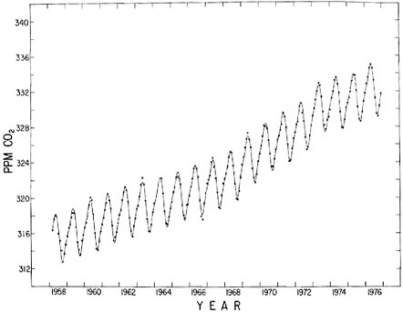
FIGURE 4.1 Trend in the concentration of atmospheric CO2 at Mauna Loa Observatory, Hawaii, at 19.5° N, 155.6° W (Keeling et al., 1976b and to be published). The dots indicate the observed monthly average concentration based on continuous measurements. The oscillating curve is a fit of the average annual variation superimposed on a spline function representation of the seasonally adjusted secular trend. The spline function was derived by the method of Reinsch (1967).
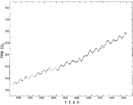
FIGURE 4.2 Trend in the concentration of atmospheric CO2 at the South Pole (Keeling et al., 1976a and to be published). The dots indicate monthly averages based on flask analyses, except for 1961 through 1963 for which monthly averages based on continuous measurements are plotted. The oscillating curve is a fit of the average annual variation superimposed on a spline function representation of the seasonally adjusted trend.
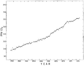
FIGURE 4.3 Seasonally adjusted concentration of atmospheric CO2 at Mauna Loa Observatory, Hawaii. Dots indicate seasonally adjusted monthly averages. The smooth curve indicates the spline function used to derive the curve in Figure 4.1.
based on the records for Hawaii and the South Pole combined (see Figure 4.6 and Table 4.1). This variability clearly reflects the approximately four-year periodicity already noted.
The airborne fraction averaged over 15 years of record, 1951 through 1973, is computed to be 56 percent. This estimate may, however, be in error by as much as 10 percent because of variability in the atmospheric data and possible
TABLE 4.1 Atmospheric CO2 Budget
|
Year |
Observed CO2 Increasea(ppm) |
Fossil Fuel Input (ppm)b |
Airborne Fraction (%) |
|
1955 |
|
0.98 |
|
|
1956 |
|
1.03 |
|
|
1957 |
|
1.08 |
|
|
1958 |
(0.89) |
1.10 |
(81) |
|
1959 |
0.80 |
1.15 |
70 |
|
1960 |
0.55 |
1.19 |
46 |
|
1961 |
0.90 |
1.24 |
73 |
|
1962 |
0.76 |
1.30 |
58 |
|
1963 |
0.50 |
1.38 |
36 |
|
1964 |
0.40 |
1.46 |
27 |
|
1965 |
0.90 |
1.52 |
59 |
|
1966 |
0.76 |
1.60 |
48 |
|
1967 |
0.68 |
1.63 |
42 |
|
1968 |
0.98 |
1.73 |
57 |
|
1969 |
1.51 |
1.83 |
83 |
|
1970 |
1.31 |
1.97 |
66 |
|
1971 |
0.85 |
2.04 |
42 |
|
1972 |
1.47 |
2.12 |
69 |
|
1973 |
1.41 |
2.26 |
62 |
|
1974 |
(0.45) |
2.26 |
|
|
1975 |
|
2.26 |
|
|
1959–1973 (inclusive) |
13.78 |
24.42 |
56.43 |
|
aAverage of the seasonally adjusted records of Mauna Loa Observatory and the South Pole as plotted in Figures 4.3 and 4.4. 1958 is estimated; 1974 is preliminary. bAs fraction of atmosphere × 106, Annual production of CO2 in grams of carbon per year (see Table 4.2 for sources of data) was converted to ppm by multiplying by the factor 290 ppm/(Nuo + Nlo), consistent with the numerical values of model parameters listed by Bacastow and Keeling (1973, p. 133). |
|||
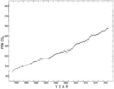
FIGURE 4.4 Seasonally adjusted concentration of atmospheric CO2 at the South Pole. Dots indicate seasonally adjusted monthly averages based on flask samples or continuous measurements as in Figure 4.2. The smooth curve indicates the spline function used to derive the curve in Figure 4.2.
systematic errors in computing the amount of CO2 produced from fossil fuel (Keeling, 1973).
That portion of the industrial CO2 that is not accounted for by an increase in atmospheric CO2 we infer to have been taken up by ocean water and possibly by land plants. A small additional amount may have been consumed by accelerated chemical erosion of carbonate or silicate rocks on
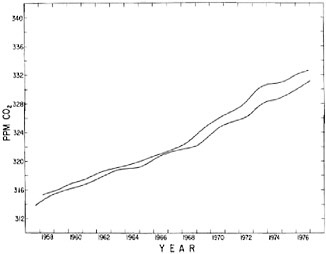
FIGURE 4.5 Comparison of seasonally adjusted trends in atmospheric CO2 for Mauna Loa Observatory, Hawaii, and the South Pole.
land. The apportioning of industrial CO2 between these carbon pools and sinks cannot easily be verified, however. No accelerated CO2 uptake is directly evident over land or in seawater. Indeed, with respect to uptake over land, no way is known to detect the small changes in storage of organic carbon that may have occurred recently as a result of an increase in atmospheric CO2 or for other reasons. A net out-
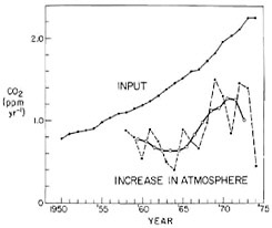
FIGURE 4.6 Upper curve: annual input of fossil fuel CO2 in the atmosphere versus time, expressed as an annual increase in concentration of atmospheric CO2 neglecting any possible removal. Lower dashed curve: annual increase of atmospheric CO2 based on the average of the secular trends for Mauna Loa Observatory, Hawaii, and the South Pole as shown in Figure 4.5. Lower full curve: four-year running mean of the annual increase as plotted by the dashed curve.
flow of carbon dioxide from land plants to the atmosphere may even have occurred in recent years (Whittaker and Likens, 1973).
With respect to uptake by seawater, direct measurements of dissolved carbon, precise enough to reveal secular changes in storage, are possible but have not been undertaken. It is therefore necessary to seek indirect estimates of industrial CO2 partitioning of which the most reliable is based on comparing radiocarbon CO2 withdrawal from the air with non-radioactive CO2 withdrawal. Revelle and Suess (1957), Broecker et al. (1971), and Machta (1973) by this method have concluded that most of the industrial CO2 leaving the air has been taken up by the oceans, with little net change in the carbon pool of land plants. In contrast, Bacastow and Keeling (1973) predicted substantial biota uptake. The issue is not settled, however, since the radiocarbon data themselves are uncertain.
4.5
PREDICTED FUTURE CO2 INCREASE IN THE ATMOSPHERE
Success in forecasting atmospheric CO2 levels over the coming decades and centuries depends on being able to estimate future fossil-fuel consumption and the fraction of fuel-derived CO2 that will remain airborne. If the world community continues to rely on the energy policies that have prevailed during the past 25 years, fossil-fuel consumption may continue to increase by as much as 4 percent per year for several more decades. On the other hand, if alternative sources of energy are found, the growth in fossil-fuel usage may soon slacken. Except for short periods, the rate will, however, probably not dip below 2 percent until well into the next century (compare Table 1.9 of Chapter 1 with Figure 4.10 below).
As for the airborne fraction, it has probably until now remained nearly constant, except for short-term variations of the kind illustrated in Figure 4.6. This is because the production of industrial CO2, although steadily rising, still amounts in total to only a minor perturbation to the natural carbon cycle. Until now, no persistent secondary interactions are likely to have complicated the primary mechanisms of atmospheric CO2 uptake. Indeed, if the adjustments of the natural carbon pools to industrial CO2 production were all small enough to be precisely linear responses in a mathematical sense, and if the nearly exponential rise in industrial CO2 input had been precisely exponential for a long time in comparison to the response times of the carbon pools, the airborne fraction would be invariant (Ekdahl and Keeling, 1973). Even as far into the future as A.D. 2000, when the CO2 input is likely to have reached 50 percent of the pre-industrial inventory, predictions based on a constant airborne fraction should still be nearly correct. On this basis, between 375 and 400 ppm of atmospheric CO2 are expected in A.D. 2000 (Machta, 1973).
Beyond A.D. 2000, the reliability in year-to-year predictions obviously diminishes. The need to predict CO2 levels correctly is, however, even greater than for this century because of the prospect of far higher CO2 levels. One approach to making such distant predictions is to fix attention on the ultimate production of CO2 and to construct simulated histories for the entire era of fossil-fuel exploitation. This requires that some new but not unreasonable assumptions be made.
The most important of these assumptions involves estimating the ultimate amount of recoverable fossil fuel. This amount is uncertain to at least a factor of 3. Hubbert (1969), whose careful estimates are by no means the highest published values (Gillette, 1974), predicts an ultimate fuel production that will yield between five and nine times the amount of CO2 in the preindustrial atmosphere. But left out of his estimates are shale oil and tar sands, which may become economical sources of fuel when more easily recovered fuels approach exhaustion. With this point in mind, Baes et al. (1976) recently estimated ultimate CO2 production from fossil fuel at 12 and Zimen and Altenheim (1973) at 13 to 14 times the preindustrial amount of CO2 Perry and Landsberg (see Chapter 1) advance a “best estimate” for ultimate fuel production slightly below Hubbert’s upper estimate but well below the other estimates quoted above.
A second important assumption relates to the rate of fuel exploitation. One cannot determine today whether fossil-fuel reserves will be processed as rapidly as economically feasible or will be stretched out by economic depressions, by wars, or by deliberate measures to conserve energy. A reasonable approach to long-range prediction is to investigate several cases so that we can appraise alternative courses of action.
An additional factor to consider is to anticipate future changes in the airborne fraction. Irrespective of the pattern of fuel use, this fraction will not remain constant during the next century, either with respect to land biota or the world oceans.
First, whether or not the land biota have recently increased their storage of carbon a few percent in response to a 10 percent rise in atmospheric CO2 level, it seems improbable that the biota will absorb more than a small fraction of the industrial CO2 near the peak stage of the fossil-fuel era because to do so would require an increase in storage of carbon of the order of the total present land biomass. Because much plant growth is limited by temperature, light, water, or nutrients rather than CO2, such a large increase seems unlikely even if the land vegetation were otherwise undisturbed by man. But since the major sources of carbon storage on land are extensive forests in Canada, Siberia, and the tropics, and since both human population and per capita consumption of natural resources are expected to increase, most of these forests will be repeatedly exploited for wood products or will be cleared of trees to produce food crops. The overall storage of carbon on land is thus likely to increase only moderately and might even decrease and add still more CO2 to the atmosphere.
Second, the oceans, although they store much more carbon than the land biota, are not able to accept large additional amounts of CO2 as easily as they accept industrial CO2
today. This is because only about 10 percent of dissolved carbon in seawater is presently in the form of ionic carbonate, and it is the presence of this chemical species that principally accounts for the oceanic uptake of CO2. As dissolved carbonate in the water is used up by reaction with industrial CO2, the CO2 pressure builds up in response to shifts in chemical equilibria among carbonate ions, bicarbonate ions, and dissolved CO2. The water is less and less able to absorb added amounts of industrial CO2. Furthermore, most seawater below a shallow surface layer exchanges with the sea surface so slowly that only the dissolved carbonate in this surface layer is readily available to react with industrial CO2. Some additional carbonate may be supplied to seawater by accelerated input from rivers, but historical rates of input (Revelle and Fairbridge, 1957) would have to be greatly increased to hold back the increase in airborne fraction significantly. Finally, accelerated dissolution of carbonate sediments on the sea floor might hold down the airborne fraction as discussed below.
A computer model that takes all these features of the carbon cycle into account has recently been investigated by Bacastow and Keeling (1973 and to be published). The ocean, atmosphere, and land biota each were divided into two reservoirs as depicted by Figure 4.7 and Table 4.2. The principal transfer coefficients for carbon exchange between reservoirs at steady state were derived from radiocarbon data or direct measurements of fluxes and abundances. The model allows for relatively rapid carbon exchange between air and the sea surface but slow exchange (1500-year mass-to-flux ratio) of deep water with surface water. The pre-industrial era turnover time for annual plants including detritus is prescribed as 2.5 years; for perennials, 60 years. A biota growth factor relates the average CO2 uptake rate of plants to the ambient CO2 concentration. This factor and the effective size of the ocean surface layer were adjusted so
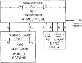
FIGURE 4.7 Six-reservoir model of the carbon cycle of Bacastow and Keeling (1973). The mass of carbon in each reservoir is represented by the Nj (t), and the transfer coefficients between reservoirs are given by the lj and kj. The magnitude of the initial values of the Nj (t) and of the time-independent values of the kj and lj are listed in Table 4.2.
TABLE 4.2 Six-Reservoir Parameters
|
Initial Values (1018 grams of carbon) |
|
|
Nuo, CO2 in stratosphere |
= 0.092 |
|
Nlo, CO2 in troposphere |
= 0.523 |
|
Nbo, carbon C in perennial biota |
= 1.56 |
|
Neo, carbon C in annual biota |
= 0.075 |
|
Nmo, inorganic and organic carbon in ocean surface layer |
= 2.46 |
|
Ndo, inorganic and organic carbon in deep ocean water |
= 36.2 |
|
Perturbation Transfer Coefficients (yr−1) |
|
|
l1, perennial biota to troposphere |
= 0 |
|
[Set to zero because the perennial plants are assumed to assimilate as well as respire carbon proportional to their mass. See Bacastow and Keeling (1973, p. 94).] |
|
|
l2, troposphere to perennial biota |
= 1/75.7 |
|
l3, annual biota to troposphere |
= 1/2.50 |
|
l4, troposphere to annual biota |
= 1/65.6 |
|
l5, stratosphere to troposphere |
= 1/2.00 |
|
l6, troposphere to stratosphere |
= 1/11.3 |
|
k3, troposphere to surface ocean |
= 1/5.92 |
|
k4, surface ocean to troposphere |
= 1/3.02 |
|
[Varies with inorganic carbon in surface ocean layer: this is initial value. See Bacastow and Keeling (1973, pp. 128– 133).] |
|
|
k5, surface ocean to deep ocean |
= 1/113 |
|
k6, deep ocean to surface ocean |
= 1/1500 |
|
Additional Model Quantities |
|
|
Г(t), industrial CO2 production |
|
|
1700 to 1860: assumed exponential increase at 4.35% per year with 1860 production of 9.53 × 10¹³ g of carbon (Keeling, 1973) |
|
|
1860 to 1969: based on annual records as cited by Keeling (1973) |
|
|
1970 to 1975: based on annual records as cited by Rotty (1976) |
|
|
After 1975: as predicted by Eq. (4.2) (see text) |
|
|
N∞, ultimate production of fossil fuel = 8.2 (Nlo+ Nuo) |
|
|
β, biota growth factor = 0.266 |
|
|
hm, depth of surface layer = 265 m |
|
that the model simultaneously predicts the observed airborne fraction based on the average of the CO2 records for Hawaii and the South Pole (see Table 4.1) and also the rate of depletion of radiocarbon by fossil fuel as deduced from studies of carbon in tree rings. Beginning in A.D. 2000, however, the biota growth factor was linearly reduced in absolute magnitude 4 percent per year, so that after A.D. 2025 the total mass of the biota remains constant. For some of the calculations, specifically noted below, the deep-water reservoir or both the surface and deep-water reservoirs were assumed to be in equilibrium with calcium carbonate since preindustrial times. For these cases, reservoir exchange of dissolved calcium as well as carbon species was taken into account and the biota growth factor readjusted to preserve agreement with the Hawaii and South Pole records. Further justification for adopting such a model is discussed in Appendix 4.A.
The production of CO2 in the past was computed from historical data (see Table 4.2). The future production of CO2
was simulated by a modified logistic function that depicts a process that initially grows exponentially in response to an almost unlimited supply of fuel but that, after proceeding long enough to decrease significantly the supply of fuel, is held back as a function of the ultimate fuel reserve remaining.
Specifically, if N is the amount of carbon in fossil fuel that has been combusted to CO2, and N∞ is the ultimate amount that will be combusted, then R(t), the relative rate of increase in N (which rate would be constant for exponential growth) is given by
(4.1)
where r is a constant chosen so that R(t) has a prescribed value for the first year of prediction. The CO2 production rate, dN/dt, simulates the characteristic rise and fall associated with growth in a limited environment. To be able to fit the curve of N versus time, t, to the recent historical period and still permit some variation in the arrival of peak values and in the steepness of rise and subsequent decline, calculations were also performed with a modified equation having an adjustable growth cutoff parameter n such that
(4.2)
Figure 4.8 shows curves that predict possible fuel combustion patterns as a result of choosing different values of the growth cutoff parameter, n. For the ultimate amount of fuel carbon, N∞, the estimate of Perry and Landsberg (see Chapter 1) was chosen as a standard case. This value is 8.2 times the amount of carbon in preindustrial CO2. A prediction of the year-to-year sequence of production close to that
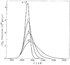
FIGURE 4.8 Industrial CO2 production in grams of carbon per year for various assumed patterns of fossil-fuel consumption. The ultimate production of industrial CO2 is fixed at 8.2 times the amount of CO2 in the preindustrial atmosphere in agreement with the best estimate of Perry and Landsberg (see Chapter 1).
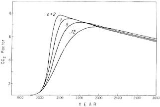
FIGURE 4.9 Predicted increase in atmospheric CO2 from A.D. 1900 to A.D. 2600. Curves are shown for the four simulated fossil-fuel consumption patterns shown in Figure 4.8. The CO2 factor expresses the amount of CO2 in the atmosphere as a multiplier of the preindustrial atmospheric CO2 abundance.
of Perry and Landsberg was obtained when the growth cutoff parameter was set at n = 0.5. The relative rate, R(t), for January 1, 1976 was set at 4.53 percent per year, consistent with the rate of increase in the annual fuel production from 1947 through 1972, a period when very nearly exponential growth prevailed.
This rate, however, is not representative of the rate for the three decades before 1945 when two world wars and a worldwide economic depression markedly slowed growth in fuel usage. The long-term average growth rate given by the product of 1/N with dN/dt for 1975 is, indeed, only 3.68 percent per year. Stated another way, setting the rate R(t) equal to 4.53 percent per year and assuming exponential growth implies that 2.22 percent of the fossil-fuel carbon ultimately available (Perry and Landsberg’s estimate) has been consumed before 1976, whereas the historic data indicate 2.82 percent. Since it makes little difference to the predicted future trend whether the former or latter fraction is used, we assumed 2.22 percent so as to provide mathematical consistency with exponential growth during the recent past.
The model predicts an initially rapid rise in atmospheric CO2 level consistent with the recent trend, a peaking sometime between A.D. 2100 and A.D. 2250, and then a period of slow decline (Figure 4.9). The pattern of fuel combustion influences the time of arrival of various levels of atmospheric CO2, and, as might be expected, the maximum CO2 level is lower if the period of combustion is stretched out. After the maximum concentration has been attained, the CO2 level falls at almost the same rate regardless of the combustion pattern chosen.
The model might be criticized for not taking into account recent perturbations in fossil-fuel production. During 1974 and 1975, the acceleration in worldwide production fell abruptly to practically zero in response to a sudden rise in the price of crude petroleum charged by the major oil exporting nations. Preliminary data for 1976 indicate, however, that
the production has once again returned to an annual growth rate near 4 percent (Rotty, 1977). This resumption may indicate that the slowdown in growth in 1974 and 1975 was only a minor perturbation to the historical long-term rising trend. For example, according to Eq. (4.2), with parameter n equal to 0.5, the relative growth rate R(t) is predicted to fall from 4.5 percent in 1976 to 4.3 percent in 1990 and 4.0 percent in A.D. 2000. Perhaps the growth in 1976 reflects a strong tendency toward adhering to this prediction. On the other hand, the resumption in 1976 may itself be an aberration with slower growth rates to return in the near future. To examine this latter possibility, we have made projections of fuel use based on the unmodified logistic Eq. (4.1) in which the rate R(t) for 1976 was varied (Figure 4.10). The corresponding atmospheric CO2 levels are shown in Figure 4.11. Although the curves are somewhat flatter near the maximum than for the earlier cases where the parameter n was varied, the differences in pattern are not very significant. Either set of curves falls well within the limits of predictability of fuel-consumption patterns. Since the assumption of steady growth is consistent with nearly three decades of recent historical record, we prefer to use Eq. (4.2) with parameter n varied from case to case and to ignore the very recent aberrations in trend.
A striking finding of the model is the diminishing effectiveness of the oceans in removing industrial CO2 as the assumed ultimate amount of fuel rises. For example, the fraction airborne at peak concentration (with growth cutoff parameter n = 0.5) is 73 percent for an ultimate consumption, N∞, fivefold the preindustrial level of atmospheric CO2. It is 81 percent for tenfold that level, and 84 percent for fifteen-fold. The peak CO2 levels for these three cases are 4.5, 8.9, and 13.4 times the preindustrial level.
The predicted atmospheric CO2 levels shown in Figure 4.9 are altered considerably if appreciable amounts of sedimentary carbonate on the sea floor are assumed to dissolve and furnish additional carbonate ions to the seawater. In deep
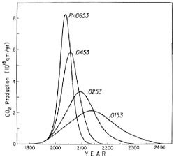
FIGURE 4.10 Additional patterns of industrial CO2 production, similar to Figure 4.8 except that the growth in rate of fuel combustion, R(t), for 1976, has been varied with logistic cutoff parameter, n, equal to unity, instead of varying n with R(t) fixed. The curve labeled R = 0.0453 is the same as that labeled n = 1 in Figure 4.8.
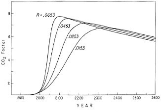
FIGURE 4.11 Predicted increase in atmospheric CO2 from A.D. 1900 to A.D. 2600 based on simulated fossil-fuel consumption patterns shown in Figure 4.10. The CO2 factor has the same meaning as for Figure 4.9.
ocean water, marine carbonates are likely to dissolve as soon as industrial CO2 reaches these waters because, even under normal conditions, most solid carbonate particles dissolve on reaching the deeper ocean basins, and their carbonate ions are returned to the water column above by the deep-water circulation. During the industrial CO2 era, an accelerated dissolution is likely to occur and perturb this otherwise nearly steady-state condition, but this tendency is reduced by the slowness with which deep water exchanges with the ocean surface.
If dissolution of shallow marine carbonates should also occur, the removal of industrial CO2 from the air would proceed rapidly because of the proximity of the overlying waters to the air-sea boundary. Arguing against this possibility is the generally high degree of supersaturation of surface water with respect to carbonates (Revelle and Fairbridge, 1957; Edmond and Gieskes, 1970; Ingles et al., 1973). Pure calcite will probably not dissolve appreciably in near-surface seawater even at the time of highest atmospheric CO2 when the pH of the water might drop as low as 7.4. More soluble high-magnesium carbonates might dissolve but probably only near the peak of industrial CO2 production. The still more soluble carbonate mineral, aragonite, is abundant in shallow tropical seas, and some aragonite is likely to dissolve during the next century. It is doubtful, however, whether there is enough of this mineral available to reduce atmospheric CO2 levels more than a few percent.
The range of possibilities for dissolution of marine carbonate to remove industrial CO2 from the atmosphere is illustrated by three predictions, shown in Figure 4.12. If only deep-water dissolution occurs, the CO2 level for several centuries is only slightly lower than if no dissolution occurs. Gradually, however, the influence of dissolution becomes evident, so that 1500 years from now, the CO2 level will have fallen to 2.6 times the preindustrial level instead of 3.9 times, as otherwise predicted. The dissolved carbon in seawater will have in-
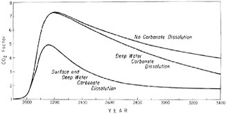
FIGURE 4.12 Predicted in crease of atmospheric CO2 from A.D. 1900 to A.D. 3500 with and without dissolution of carbonate sediments. The pattern of fossil-fuel consumption is as shown by the case n = 0.5 of Figure 4.8. The CO2 factor has the same meaning as for Figures 4.9 and 4.11.
creased by 19.0 percent of the preindustrial concentration (instead of 8.3 percent), and carbonate sediment will have been removed from the ocean floor to a global average depth of about 3 cm.
If dissolution occurs throughout the fossil-fuel era in both shallow and deep water, the atmospheric CO2 is noticeably lower than otherwise, even as early as the next century. The level in A.D. 3500 will have fallen to only 1.7 times the preindustrial level with most of the falloff before A.D. 2500. The increase in dissolved carbon in seawater in the ocean as a whole will be 22.5 percent of the preindustrial concentration. This amount is not much greater than if dissolution of carbonate occurs only in deeper water (19.0 percent), but in this case, 98 percent of the carbonate that dissolves will have been stripped out of shallow-water sediments. Most of this carbonate, of course, does not remain in surface water: by A.D. 3500 all but 7 percent will have transferred to deep water, principally as dissolved bicarbonate. The average depth of shallow-water carbonate sediment removed from the ocean floor will be the order of 40 cm. Since far less than half of the area of shallow seas contains carbonate-rich sediment, several meters of such sediment on average will have to be stripped of carbonate. This sediment thickness is so great that it seems highly unlikely that extensive dissolution can occur in shallow water within 1500 years even if undersaturation occurs. Thus, the third prediction seems considerably less likely to be fulfilled than the second. Regardless of which prediction is chosen, however, the level of atmospheric CO2 is predicted to remain near or higher than twice the preindustrial level for a thousand years.
These predictions all assume that the land biota carbon pool is not substantially altered during this long period. If the biomass grows throughout the fossil-fuel era approximately in proportion to the increase in atmospheric CO2, as assumed in the present model up to A.D. 2000, the predicted atmospheric CO2 level not only is substantially lower than otherwise near the period of peak concentration but thereafter falls relatively rapidly to near present levels while the biota carbon pool more than doubles. Although this possibility cannot be ruled out on the basis of present limited knowledge of land plant response to CO2, there is little positive evidence to support it. The subject is further discussed in Appendix 4.A below.
Lesser but substantial uptake of CO2 by land plants is also possible but still requires a large fractional increase in biotic carbon storage. Since the ultimate amount of recoverable fossil fuel is also uncertain to at least the order of the amount of carbon stored by the land biota, the predicted levels of CO2 over the next thousand years remain quite uncertain. The present discussion principally emphasizes that the world’s oceans cannot be expected to remove a major fraction of the industrial CO2 from the air for a long time in comparison with the lifetime of human institutions. Although other mechanisms of CO2 withdrawal may exist, it is probably prudent to expect the concentration of atmospheric CO2 to persist above twice the preindustrial level for at least several centuries.
If Manabe’s prediction of atmospheric temperature rise should be close to correct, even a doubling of the CO2 level is likely to product climatic change. Manabe’s climatic model gives no insight into the importance of the duration of high CO2 levels, but it seems reasonable that a long period of high CO2 is more likely to lead to climatic change than would a shorter-term perturbation. As for the ultimate restoration of the ocean and atmosphere to their preindustrial condition, this will require reprecipitation of the carbon added to the ocean water as a result of industrial CO2 uptake. This is likely to occur only if the world’s rivers transport enough noncalcareous alkaline salts to the oceans to neutralize the acidic capacity of the industrial CO2 already added to the oceans. These salts can only be derived from the decomposition of noncarbonate rocks and soils, and this weathering process probably requires not less than 10,000 years to bring about a major part of the restoration.
REFERENCES
Augustsson, T., and V. Ramanathan (1977). The radiation convective model study of the CO2 climate problem, J. Atmos. Sci. 34, 448.
Bacastow, R. B. (1976). Modulation of atmospheric carbon dioxide by the southern oscillation, Nature 261, 116.
Bacastow, R. B., and C. D. Keeling (1973). Atmospheric carbon dioxide and radiocarbon in the natural carbon cycle; Changes from A.D. 1700 to 2070 as deduced from a geochemical model, in Carbon and the Biosphere, G. M. Woodwell and E. V. Pecan, eds., U.S. Atomic Energy Commission, pp. 86–135.
Bach, W. (1976). Global air pollution and climatic change, Rev. Geophys. Space Phys. 14, 429.
Baes, C. F., Jr., H. E. Goeller, J. S. Olson, and R. M. Rotty (1976). Carbon dioxide and climate: the uncontrolled experiment, submitted to American Scientist.
Bischof, W. (1973). Carbon dioxide concentration in the upper troposphere and lower stratosphere. III, Tellus 25, 305.
Bolin, B., and W. Bischof (1970). Variations of the carbon dioxide content of the atmosphere in the northern hemisphere, Tellus 22, 431.
Broecker, W. S., Y.-H. Li, and T.-H. Peng (1971). Carbon dioxide—man’s unseen artifact, Chapter 11 of Impingement of Man on the
Oceans, D. W. Hood, ed., Wiley-Interscience, New York, pp. 287–324.
Committee on Impacts of Stratospheric Change (1976). Halocarbons: Environmental Effects of Chlorofluoromethane Release, National Academy of Sciences, Washington, D.C.
Edmond, J. M., and J. M. T. M. Gieskes (1970). On the calculation of the degree of saturation of sea water with respect to calcium carbonate under in situ conditions, Geochim. Cosmochim. Acta 34, 1261.
Ekdahl, C. A., and C. D. Keeling (1973). Atmospheric CO2 and radiocarbon in the natural carbon cycle: I. Quantitative deduction from the records at Mauna Loa Observatory and at the South Pole, in Carbon and the Biosphere, G. M. Woodwell and E. V. Pecan, eds., U.S. Atomic Energy Commission, pp. 51–85.
Flohn, H. (1975). History and intransitivity of climate, appendix 1.2 in The Physical Basis of Climate and Climate Modelling, Report of the International Study Conference in Stockholm, July 29–August 10, 1974, GARP Publication Series No. 16, World Meteorological Organization, Geneva, pp. 106–118.
Gillette, R. (1974). Oil and gas resources: Did USGS gush too high? Science 185, 127.
Hubbert, M. K. (1969). Energy resources, Chapter 8 of Resources and Man, the Division of Earth Sciences, National Academy of Sciences, Washington, D.C., pp. 157–242.
Ingles, S. E., C. H. Culberson, J. E. Hawley, and R. M. Pytkowicz (1973). The solubility of calcite in sea water at atmospheric pressure and 35% salinity, Marine Chem. 1, 295.
Keeling, C. D. (1973). Industrial production of carbon dioxide from fossil fuels and limestone, Tellus 25, 174.
Keeling, C. D., J. A. Adams, C. A. Ekdahl, and P. R. Guenther (1976a). Atmospheric carbon dioxide variations at the South Pole, Tellus 28, 552.
Keeling, C. D., R. B. Bacastow, A. E. Bainbridge, C. A. Ekdahl, P. R. Guenther, L. S. Waterman, and J. S. Chin (1976b). Carbon dioxide variations at Mauna Loa Observatory, Hawaii, Tellus 28, 538.
Kelley, J. J., Jr. (1969). An analysis of carbon dioxide in the Arctic atmosphere near Barrow, Alaska, 1961 to 1967, Scientific Report, Office of Naval Research, Contract N00014-67-A-0103-0007, NR 307-252.
Lowe, D. C. (1974). Atmospheric carbon dioxide in the southern hemisphere, Clean Air, February, 12.
Machta, L. (1973). Prediction of CO2 in the atmosphere, Carbon and the Biosphere, G. M. Woodwell and E. V. Pecan, eds., U.S. Atomic Commission, pp. 21–31.
Manabe, S., and R. Wetherald (1967). Thermal equilibrium of the atmosphere with a given distribution of relative humidity, J. Atmos. Sci. 24, 241 –259.
Manabe, S., and R. Wetherald (1975). The effects of doubling the CO2 concentration on the climate of a general circulation model, J. Atmos. Sci., 32, 3–15.
McElroy, M. B., J. W. Elkins, S. C. Wofsy, and Y. L. Yung (1976). Sources and sinks for atmospheric N2O, Rev. Geophys. Space Phys. 14, 143– 150.
Newell, R. E., and B. C. Weare (1977). A relationship between atmospheric carbon dioxide and Pacific sea surface temperature, Geophys, Res, Lett. 4, 1.
Pearman, G. I., and J. R. Garratt (1973). Space and time variations of tropospheric carbon dioxide in the southern hemisphere, Tellus 25, 309.
Ramanathan, V. (1976). Greenhouse effect due to chlorofluorocarbons; climatic implications, Science 190, 50.
Reinsch, C. H. (1967). Smoothing by spline functions, Num. Math. 10, 177.
Revelle, R., and R. Fairbridge (1957). Carbonates and carbon dioxide, Treatise Marine Ecol. Paleoecol 1, 239.
Revelle, R., and H. E. Suess (1957), Carbon dioxide exchange between atmosphere and ocean, and the question of an increase of atmospheric CO2 during the past decades, Tellus 9, 18.
Rotty, R. (1976). Paper prepared for the Conference “Fate of Fossil Fuel CO2,” Honolulu, January 19–23, N. R. Andersen and A. Malahoff, eds., to be published by the Office of Naval Research, Dept. of the Navy, Arlington, Va.
Rotty, R. (1977). Present and future production of CO2 from fossil fuels—a global appraisal, paper prepared for Energy Research and Development Agency (ERDA) Workshop on Significant Environmental Concerns, Miami, Florida, March 7–11.
Schneider, S. H. (1975). On the carbon dioxide-climate confusion, J. Atmos, Sci. 32, 2060.
Sze, N. D. (1977). Anthropogenic CO emissions: implications for the atmospheric CO-OH-CH4 cycle, Science 195, 673.
Wang, W. C., Y. L. Yung, A. A. Lacis, T. Mo, and J. E. Hansen (1976). Greenhouse effects due to man-made perturbations of trace gases, Science 194, 685.
Weiss, R. F., and H. Craig (1976). Production of atmospheric nitrous oxide by combustion, Geophys. Res. Lett. 3, 751.
Whittaker, R. H., and G. E. Likens (1973). Carbon in the biota, in Carbon and the Biosphere, G. M. Woodwell and E. V. Pecan, eds., U.S. Atomic Energy Commission, pp. 281– 302,
Yung, Y. L., W. C. Wang, and A. A. Lacis (1976). Greenhouse effect due to atmospheric nitrous oxide, Geophys. Res. Lett. 3, 619.
Zimen, K. E., and F. K. Altenheim (1973). The future burden of industrial CO2 on the atmosphere and the oceans, Naturwissenschaften 60, 198.
APPENDIX 4.A:
ASSESSMENT OF SIX-RESERVOIR MODEL TO DEPICT FUTURE ATMOSPHERIC CO2 ABUNDANCES
INTRODUCTION
The global geochemical exchange system recently perturbed by industrial CO2 production is described above by means of a model with six generalized reservoirs that store and exchange CO2. It is important to ask whether this model is adequate to the task of predicting future atmospheric CO2 levels. The following discussion will attempt, at least in part, to answer this question. The six-reservoir model, shown in Figure 4.7 of the main text, will be referred to below as the “6R” model.
This 6R model is representative of a class of models, called “reservoir” or “box” models, which are designed to focus on chemical exchange between various sectors or ‘“pools” of a biogeochemical system. Such models are suited to solving critical problems of chemical transport arising at the boundaries between pools without dealing with mechanisms of transport or storage within these pools. Because of their simplicity, box models are convenient for solving time-dependent problems. The absence of internal complexity promotes freedom to address details of time dependency.
To appreciate the advantages and weaknesses of box models, their most important general properties will now be considered. Afterward, critical aspects of modeling the land
biota and ocean water will be discussed in terms of the 6R and selected alternative models.
BOX MODELS
A box model describes a system of reservoirs in which the behavior of a trace chemical substance is described principally or solely in terms of its rate of entering and escaping from each reservoir. A reservoir boundary may be a clearly defined physical surface, such as an air-sea boundary, or it may merely divide regions into convenient subregions, such as shallow and deep-ocean water. Within the volumes described by these boundaries only averages or totals of the properties of the reservoir are considered.
In a box model, the flux of chemical tracer emerging from a reservoir is typically assumed to vary with time in proportion to time changes in the total amount, or mass, of tracer within that reservoir. Specifically, if N denotes the mass of tracer and J the flux out:
(4.A.1)
where J0, N0, and k are constants. The flux and mass constants, J0 and N0, often represent steady-state or initial values for the tracer of interest. The ratio N/J is often called a turnover or residence time, and k a box-model exchange coefficient.
For purposes of this discussion, a model in which all the reservoirs are assumed to obey Equation (4.A.1) will be called a “simple box model.”
With the great majority of simple box models, it is further assumed that the turnover time is a constant defined by the steady-state ratio N0/J0, i.e.,
(4.A.2)
whence
(4.A.3)
A constant turnover time implies that the distribution of tracer and its circulation within the reservoir (if it circulates) are such that every atom or molecule of tracer in the reservoir has the same chance of escaping at any moment regardless of how or where it entered or where it has resided or circulated within the reservoir. One might say that the tracer is assumed to be randomly distributed or randomly mixed.
This assumption may not be realistic, but it is typically more reasonable than to assume that a tracer is uniformly or well mixed, as is often demanded. Furthermore, if a tracer’s actual behavior inside a reservoir is poorly understood, a random escape mechanism may be the most reasonable hypothesis by default. At least, such a model does not assume details that are unknown.
If a random escape mechanism is a poor representation of the real system of interest, Eq. (4.A.3) is likely to be untrue. Nevertheless, Eq. (4.A.1) may still be a good approximation of the tracer transport if the flux and the mass vary so slightly from their steady state values, J0 and N0, that these variations are essentially first-order perturbations. To demonstrate this it is only necessary to assume that J is related to N by a function
(4.A.4)
which possesses derivatives, f′, f″, …, with respect to N. Expanding f in a Taylor’s series:
(4.A.5)
where J0 is equal to f(N0). Equation (4.A.1) holds whenever the second- and higher-order perturbation terms are sufficiently small to be neglected.
For additions of industrial CO2 to the earth’s natural carbon pools, the fractional increases in carbon in the reservoirs are, up to the present time, only a few percent. Thus Eq. (4.A.1) is likely to be a reasonable approximation irrespective of the true functional relationships of mass and flux within the reservoirs.
Furthermore, if the assumption of random escape is known to be false for a box-model reservoir, the modelist often may be able to subdivide the reservoir to conform better with the known facts. Subdivisions need not even be physically distinct; they may share the same environment. For example, annual and perennial plants exchange comparable amounts of carbon dioxide with the atmosphere, but perennials store many times more carbon. Obviously, the carbon atoms of annuals and perennials have distinctly different chances of returning to the atmosphere. By modeling the land biota as two reservoirs, as was done with the 6R model, this fact can be accounted for even though annual and perennial plants intermingle. Moreover, there is no obligation to divide the biota precisely in terms of annuals and nonannuals, nor need a distinction be made as to whether the short-cycled material is derived solely from short-lived plants or includes material, such as the leaves, of long-lived plants. One can assign any convenient pair of turnover times to define the portions (cf. Keeling, 1973, p. 306).
Reservoir subdivision need not stop at two portions. With respect to the land biota, for example, categories such as annuals, biennials, perennials, deep humus, and peat might all be distinguished. In principle, the modelist could even dispense altogether with a finite number of subdivisions and describe the distribution of the outgoing tracer flux of the entire reservoir as a continuous function with respect to turnover time. Some years ago this approach was proposed by Eriksson and Welander (1956) for the land biota.
Following their lead, let us formulate a generalized box model in which the amount of tracer, N, in a given reservoir (such as the entire land biota) varies with time, t, by an expression of the form
(4.A.6)
where N0 denotes an initial unperturbed value of N. The function, g(t), will denote the departure from an initial unperturbed steady state of the tracer flux into that reservoir; and the dimensionless “transfer” function, ![]() will describe how molecules or atoms of tracer in that input flux are distributed with respect to the time interval,
will describe how molecules or atoms of tracer in that input flux are distributed with respect to the time interval, ![]() in which they are expected to remain in that reservoir, i.e.,
in which they are expected to remain in that reservoir, i.e., ![]() denotes the fraction of molecules or atoms entering the reservoir at time t that are still in the reservoir at time
denotes the fraction of molecules or atoms entering the reservoir at time t that are still in the reservoir at time ![]() The integral of Eq. (4.A.6) thus keeps track of the total increase or decrease in mass of tracer within the reservoir in terms of how much tracer enters and leaves the reservoir at the boundaries after some initial time, t = 0.
The integral of Eq. (4.A.6) thus keeps track of the total increase or decrease in mass of tracer within the reservoir in terms of how much tracer enters and leaves the reservoir at the boundaries after some initial time, t = 0.
This integral is a convolution integral. It follows that the Laplace transform of N is equal to the product of the transforms of f and g. The analytic solution of Eq. (4.A.6) is often facilitated by the use of such transforms.
The transfer function for a reservoir of a simple box model has the form (Eriksson, 1961)
(4.A.7)
where k is the ratio of change in mass to change in flux defined by Eq. (4.A.1.). For a reservoir such as the land biota, subdivided into two parts with respect to turnover time, the transfer function of the biota as a whole takes the form
(4.A.8)
where f1 + f2 = 1. By a proper choice of k1, k2, and f1/f2, this function can approximate a considerable range of possible real cases. Analogous expressions apply to subdivision into more than two portions.
More generally, the transfer functions of box models may be of almost any functional form and may even be time-dependent. Models so formulated are not entirely general, however. Equation (4.A.6) requires that there be a linear relationship between the input g(t) and the response N(t), i.e., if g(t) is represented as the sum of very short duration impulses or “spikes” of tracer, then N can be constructed by superposition of responses to these impulses.
Such linearity may not be realistic especially for large perturbations. For example, if the biota should turn over carbon at a different average rate in the next century because of changes in the size of the biota, the biotic response to a single spike would be different than for a series of spikes. In this case, the time dependency of ![]() cannot be specified in advance since it depends on the character of the source. A convolution integral is then not the most appropriate means of solving the problem of interest. Other approaches, for example involving nonlinear differential equations, may be more suitable.
cannot be specified in advance since it depends on the character of the source. A convolution integral is then not the most appropriate means of solving the problem of interest. Other approaches, for example involving nonlinear differential equations, may be more suitable.
Another complication arises if several geochemical reservoirs interact, as is the case for the atmosphere, oceans, and land biota. The tracer output flux of one reservoir becomes the input to another reservoir, and more than one reservoir boundary may have to be distinguished.
In modeling the fossil-fuel CO2 problem, only the atmospheric reservoir unavoidably presents the problem of possessing outputs that are also the inputs to other reservoirs. Fortunately for the modelist, the atmosphere’s steady-state internal mixing time is short compared with the characteristic time for industrial CO2 input. Only small errors arise if industrial CO2 is assumed to mix randomly or thoroughly in the atmosphere, and Eq. (4.A.1) for the atmosphere holds for large perturbations as well as small ones. The industrial CO2 input, g(t), to other reservoirs in contact with the atmosphere can therefore be expressed as the product of an exchange coefficient and the globally averaged change in atmospheric CO2, as in a simple box model. The latter change in turn can be computed in a simple manner knowing the transfer functions f(t) of these other reservoirs. [This is shown in the discussion following Eq. (4.A.13), below.]
If the oceans are divided into a surface and deep layer as in the 6R model, the surface layer presents a separate boundary and a coupled input and output between that layer and the ocean below. If the surface layer is not assumed to be deeper than the physically well-mixed layer of the real oceans (about 75 m), the assumption of a randomly mixed layer obeying Eq. (4.A.3) would be reasonable except that at the air-sea boundary chemical complications arise that require that Eq. (4.A.1) be used. If the surface-layer reservoir is assumed to be deeper than about 75 m, even Eq. (4.A.1) should not be assumed to be a good approximation except for small perturbations. Either a more realistic model should be devised or the approximation demonstrated to be satisfactory for the particular calculation of interest.
With this general view of box models and their capabilities as background, the modeling of the land biota and oceans will now be discussed in relation to the formulation of the 6R model.
LAND BIOTA
The division of the land biota into two carbon pools in the 6R model has already been explained as stemming from a disparity between the fluxes and storage times for long and short-cycled species. Keeling (1973, pp. 305– 309) discusses the limitations of the data base on which this disparity is established. Additional subdivision would have added computational complexity without improving the prediction of future atmospheric CO2 levels.
Deep-soil humus and incipient geological deposits such as peat were left out of the model since these carbon pools turn over so slowly that they are likely to be negligibly perturbed by any biotic response to changing atmospheric CO2 levels at least for several more decades. Furthermore, no model based on present knowledge is likely to predict adequately their behavior over longer time periods.
The short-cycled biota carbon pool is assumed initially to contain 4.6 percent of the total biotic carbon but to contribute 54 percent of the carbon exchange with the atmosphere. The remaining flux and mass are attributed to the long-cycled carbon pool. The turnover times of the respective pools are 2.5 and 60 years. No distinction is made between
living and dead materials because exchange between these categories is expected to have little influence on the exchange processes of interest.
Because so little carbon is stored in the short-cycled biota, atmospheric CO2 predictions are almost indistinguishably altered if this carbon pool is neglected altogether as was done by Oeschger et al. (1975). The modeling of the biota as two reservoirs thus has the practical effect of discounting the overall biotic uptake of carbon by about one half while maintaining the assumed biotic storage capacity nearly intact.
The transient increase in biotic uptake of CO2 in the 6R model is made proportional to the logarithm of the increase in atmospheric CO2 concentration above the preindustrial concentration. This relationship has been found for individual plants grown in greenhouses (see Keeling, 1973, for original references). The proportionality constant, called a “biota growth factor,” was set, as described in the next section, to predict the observed increase in atmospheric CO2 over the period of direct measurements, 1959 to 1974. The logarithmic function predicts a gradual cutoff of biotic increase at high ambient CO2 levels but very nearly directly proportional response to the small CO2 rise that has occurred so far. The model provides that the uptake and release of CO2 by the long-cycled biota pool depend directly on pool size as well, on the grounds that the leaf area of plants will increase in proportion to total mass, that fixation of CO2 per unit leaf area will remain constant, and that plants will respire CO2, and dead materials will decay, in proportion to total mass. None of these assumptions is based on hard evidence. Each merely reflects what would seem reasonable for small perturbations.
For the period 1959 to 1974, and on the assumption either that no carbonate dissolves in the oceans or that carbonate dissolves only in the deep oceans, the 6R model predicts that the biota, short and long cycled combined, increase by 0.63 percent. If dissolution occurs in the surface layer of the oceans, the biota pool size remains almost constant. If the entire past industrial period up to 1974 is considered, the predicted biota increase does not exceed 1.7 percent. These changes are far too small to be directly detectable but, being small, make reasonable the above-mentioned assumptions of the model.
For large atmospheric CO2 perturbations of the global biota, no trustworthy observations or theories exist to guide the modelist. The calculations described in the main text of this chapter reflect the view that large increases in the biota will not occur because loss of virgin lands to agriculture and widespread increase in density of human settlement with its attendant disturbance of soils will prevent any major future global buildup of organic carbon. In the 6R model, the biotic increase is simply brought to a halt by an external computer program command. For the case of an ultimate industrial CO2 production of 8.2 times the preindustrial atmospheric CO2, a logistic parameter n of 0.5, and either no carbonate dissolution or carbonate dissolution only in the deep oceans, the biota carbon pool is predicted to have increased by 5.9 percent in 2025, after which time its size remains constant. If dissolution also occurs in the surface layer, the biotic pool is predicted to decrease very slightly (by −0.1 percent).
Since these small changes in the biota hardly influence the atmospheric CO2 concentration near or after the time of peak levels, the biota carbon pool could be left out of the 6R model altogether were it not that its presence provides a basis for explaining part of the withdrawal of CO2 from the atmosphere during the historical record period, 1959 to 1974. With the biota included, the modelist may adjust the model to agree with these observations without being obliged unrealistically to adjust the oceanic parameters to account exactly for the industrial CO2 uptake.
Only if our understanding of the biota response to industrial CO2 improves in the coming years will the inclusion of biota reservoirs in predictive models become truly useful. This is especially true for the large biotic carbon pools, such as deep-soil humus, which turn over very slowly under natural conditions.
Finally, it should be pointed out that Machta (1971) and Oeschger et al. (1975) modeled the biota with a transfer function that provides that each molecule of CO2 entering the biota will escape after exactly the average turnover time of carbon in the reservoir. In the case for which the atmospheric CO2 concentration rises exponentially, say at a rate proportional to eµl, their models yield the same prediction for biota growth as the 6R model does, provided that the 6R model growth factor is replaced by their growth factor multiplied by (1 − e−60µ) where 60 years is their assumed value of the biotic carbon turnover time. For the approximate exponential growth in industrial CO2 since 1945, µ−1 is approximately 22 years, and this adjustment factor is about 0.93. Since neither their models nor the 6R model were used to consider biota increases after nearly exponential rise in CO2 has ceased, it is not worthwhile to discuss their biota model in any greater detail here.
THE OCEANS
The division of the ocean into layers for chemical modeling purposes was first investigated in detail by Craig (1957). The turnover time of the whole ocean, if computed from the steady-state flux of radiocarbon at the air-sea boundary, is about 400 years, whereas the average circulation time based on radioactive tracer studies is known to be greater than 1000 years. As Craig pointed out, such a discrepancy can be accounted for by a simple box model with two tandem oceanic reservoirs. A surface layer of almost any depth up to several hundred meters might be assumed. Craig, however, made a physically realistic choice by fixing the model depth at 75 m to agree approximately with the average depth of the seasonal thermocline above which the water is vertically well mixed. Although the Craig model is a good approximation for this surface layer, it is a gross oversimplification for the water lying below. This is because a transition zone, defined by a steep temperature gradient, divides this surface layer from the relatively homogeneous deep ocean below 1000 m [see, for example, von Arx (1974),
Figure 5.5, p. 131]. An oceanic model could be devised with more than two vertically separated reservoirs to account for the transition zone, but further subdivision, as in the case of the biota, does not necessarily lead to a better model, because available observational data offer a poor basis for establishing the additional transport parameters required. On the other hand, if the ocean is divided vertically into only two reservoirs, the dividing surface is more reasonably located somewhere near the middle of the subsurface transition zone rather than at its top.
As a basis for assigning a depth greater than the physically defined mixed layer, Bacastow and Keeling (1973) forced the 6R model to predict the Suess effect, i.e., the dilution of atmospheric radiocarbon by industrial CO2 up to 1954 when nuclear-weapons testing began to alter the natural radiocarbon cycle. The significance of this approach to calibration of the 6R model will now be considered in some detail, first in terms of the 6R model and a simplified version of it, the “4R” model, and second in terms of a generalized box model. The discussion will rely in part on a recent investigation of the CO2 modeling problem by Oeschger et al. (1975).
THE SUESS EFFECT
Because industrial CO2 contains no radiocarbon, its injection into the air dilutes the atmospheric radiocarbon residing there naturally as a result of cosmic-ray production. Were it not for the ability of the biota and oceans to store radiocarbon and for the chemical reactivity of seawater to inhibit the oceanic uptake of industrial CO2, the relative decrease in radiocarbon would be almost exactly equal to the relative increase in atmospheric CO2. Actually, the Suess effect, as observed in tree rings that grew around 1950, is approximately one third of the CO2 increase at that time.
This is a result of two factors. First, the Suess effect is smaller than otherwise because the land biota carbon pool dilutes radiocarbon. This dilution is nearly independent of small changes in the size of the biotic carbon pool. On the other hand, small changes in pool size may have appreciably increased or decreased the abundance of atmospheric CO2.
Second, with respect to the chemical reactivity of seawater, a thermodynamic restraint inhibits the oceanic uptake of atmospheric CO2 while scarcely influencing the radiocarbon distribution. Because the storage of carbon in the oceans is expressed in terms of total dissolved carbon in seawater, whereas gas exchange at the air-sea boundary depends on the partial pressure gradient at that boundary, the steady-state box model exchange coefficient, kma, for the escape of CO2 from the surface oceanic layer to the atmosphere must be multiplied by a perturbation factor to account properly for transient exchange. This factor is defined as the ratio of the relative change in CO2 pressure exerted by the water to the relative change in total carbon in the water. Bacastow and Keeling (1973) calculated its value without approximation from known (if somewhat uncertain) thermodynamic constants for seawater. They called it an “evasion factor” (symbol, ξ). It has also been called the “Revelle factor” after the scientist who first proposed its use and noted that its present value is of the order of 10 (Revelle and Suess, 1957). Taking into account the Revelle factor reduces by this factor the otherwise predicted capacity of the surface ocean layer to store industrial CO2 but has almost no effect on the radiocarbon distribution. This is because, as with the biota, the oceans serve only to dilute radiocarbon, irrespective of the chemical reactions occurring in the reservoir.
As one might expect when two quasi-independent observations are available, a knowledge of both the observed Suess effect and the observed CO2 increase permits the CO2 uptake by the biota and that by the oceans to be separately evaluated. What is less obvious is that this evaluation is almost independent of assumptions as to how carbon circulates in subsurface ocean water and does not require that the Suess effect and the recent CO2 increase to be known for the same period.
The Suess effect around 1950 is predicted by the 6R model to be approximately −2.2 percent for a surface layer depth, hm, of 75 m. [Bacastow and Keeling (1973) give exact details.] This prediction is somewhat larger than the average observed Suess effect based on tree-ring studies, a value of about −2.0 percent. If hm is increased to 120 m, the predicted Suess effect agrees well with the observations. Observed values scatter considerably, however, and, since local industrial CO2 may have contaminated some of the samples used in the tree-ring studies, the observed value may be systematically too high. Unless all are wrong, however, the Suess effect cannot have been much smaller than the −1.4 percent value predicted if hm is set at about 700 m. A more likely value for the Suess effect is −1.8 percent. Therefore, the surface-layer depth in the 6R model should probably not be set larger than approximately 700 m, although about 250 m is probably more appropriate.
In the 6R model, in addition to the depth parameter, hm, there is another adjustable oceanic factor: the average turnover time of the deep layer. Bacastow and Keeling (1973) found (see their Figure 5) that the 6R model yields almost the same relationship for the ratio of the predicted Suess effect to the predicted atmospheric CO2 increase irrespective of which parameter is varied. Specifically, if hm is fixed at approximately 120 m and the box-model turnover time of the deep-ocean layer, kdm−1, is varied, the relation between the Suess effect near 1950 and the CO2 increase for 1959 to 1969 is almost indistinguishable from the relation found when hm is varied and kdm–1 is fixed at 1500 years.
To explain this result, it is important to note, as in the main text of this chapter, that the input of industrial CO2 has been rising almost exponentially, while past responses of the biota and oceans to this input have probably been essentially linear. Under conditions of linear response to a persistent exponentially rising input, the annual airborne fraction, i.e., the ratio of the annual atmospheric CO2 increase to the annual industrial CO2 production, is predicted by the 6R model to approach constancy with time (Ekdahl and Keeling, 1973; Oeschger et al., 1975). The cumulative airborne fraction, i.e., the ratio of the total atmospheric CO2 increase from the preindustrial value, to the cumulative CO2 production, also approaches this value.
If the magnitude of the Suess effect is divided by the cumulative industrial CO2 input, a radiocarbon dilution factor is obtained that is analogous to the cumulative airborne fraction. Like the latter, it is nearly time invariant for a linear response to an exponentially rising CO2 input. The exchange parameters to predict the dilution factor are, however, modified from those for inactive CO2, depending on the Revelle factor, ξ, and the biota growth factor (which will be denoted by the symbol β). Since ξ is known from thermodynamic data, one can adjust the unknown magnitude, β, and an additional parameter related to oceanic uptake of CO2 so that the model predicts both the radiocarbon dilution and the airborne fraction. As already stated, either of two subsurface parameters of the 6R model may be varied to produce the desired predictions.
To explain this point quantitatively, let us define a four-reservoir (4R) model in which the 6R model is simplified by combining its two atmospheric reservoirs and eliminating its short-cycling biota reservoir. Also, the long-cycled biota will be assumed to exchange as in a simple box model, i.e., CO2 uptake will depend only on changes in atmospheric CO2 not on biota pool size as well. For this 4R model, as with the 6R model, the assumed depth of the surface layer and the average turnover time of the deep layer are critical for establishing the predicted magnitude of the airborne fraction and radiocarbon dilution.
Specifically for the 4R model, if the Revelle factor, ξ, is assumed constant, and if the industrial CO2 input to the atmosphere, ga(t), rises exponentially with time as predicted by the equation
(4.A.9)
and if t is long compared to the efold time µ−1, the airborne fraction, is (cf. Ekdahl and Keeling, 1973)
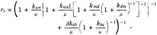
(4.A.10)
where the simple box-model exchange coefficients are as defined in Table 4.A.1.
The indices have the following significance: a, atmosphere; b, biota; m, oceanic surface layer; d, deep ocean. The exchange coefficient, kij, refers to transfer from reservoir i to reservoir j. All kij are assumed to be constant with time.
This expression is of the form
(4.A.11)
where A, B, and C have fixed values for a constant value of the efold time, µ−1 The quantities, A, C, and ξ are reasonably well known compared with B and β. Therefore, the latter may be justifiably regarded as the unknowns to be evaluated from the time-dependent observations.
The corresponding radiocarbon dilution factor, for the 4R model, is to a close approximation (cf. Oeschger et al., 1975, p. 181) given by
(4.A.12)
where the influence of isotopic fractionation is neglected.
It is now possible to explain the finding of Bacastow and Keeling (1973) that a nearly unique concordance exists between the predicted Suess effect and airborne fraction. If the depth of the surface layer is varied (causing kma and kmd to vary) or if kdm is varied, holding the surface layer depth constant, a change occurs in the value of B. Irrespective of which box model parameter is changed, the change in B has the same effect on the relative values of ra and ra*.
When the actual year-to-year CO2 production data were used in the calculation, the nonlinear influence of a variable Revelle factor allowed for, and isotopic fractionation prescribed, Bacastow and Keeling found that the discrepancy between the results varying one parameter or the other was of the order of 0.04 percent in the Suess effect. This discrepancy is too small to be useful in obtaining any additional information about the 6R model over that assuming linearity and an exponential rise in CO2 production.
What has been gained by taking into account the Suess effect is solely to be able to compute separately the industrial CO2 input to the oceans and to the biota. This was done by first solving Eq. (4.A.12) for the subsurface oceanic parameter, B, and then solving Eq. (4.A.11) for the biotic growth factor, β.
Although this separate computation of inputs has been shown only with respect to the 4R model, it applies generally. In order to show this as a prelude to considering an alternative model, the significance of the Suess effect will now be reconsidered within the framework of a model with a generalized oceanic transfer function.
THE GENERALIZED OCEANIC BOX MODEL
To keep the analysis of this general model as simple as possible, no changes will be made in the modeling of the atmosphere and land biota. These reservoirs will again be assumed to transfer and store carbon as predicted by a simple box model. As noted earlier, this is a good approximation for the atmosphere. With respect to the biota, a simple box model suffices to explain the significance of the Suess effect even if the numerical values predicted by the model are questionable because of uncertainty in the pool size and the distribution of turnover times of various sectors of the biota.
With respect to the oceans, the essential difference in uptake of industrial CO2 and radiocarbon should become evident if the subsurface ocean is regarded as being separated from the atmosphere by a thin boundary layer that interacts with the atmosphere in a manner consistent with the known chemistry of seawater and that correctly predicts the transport of carbon to and from the subsurface layer. If the boundary layer is defined to be thin enough to have negligible capacity to store carbon, the transport mechanism within the layer is not important, and a simple box model formulation will almost surely suffice. With this
view in mind the generalized oceanic model, as proposed by Welander (1959), will be assumed to possess a simple box-model boundary layer of negligible thickness. This approach is, of course, more rigorous than to assume a boundary layer of 75 m, which in reality may not fully obey the simple box-model equations.
With respect to the ocean below this boundary layer, no restriction will be placed here on the mechanism of carbon transport or storage except to assume that the same mechanism applies to both industrial CO2 and radiocarbon and that the process is linear.
The box-model exchange constants for interactions between the atmosphere, biota, and oceanic boundary layer will be formulated as before for the 4R model, i.e., the radiocarbon constant, kma, for transfer from the oceanic surface to the atmosphere will be increased for CO2 by a factor, ξ, and the radiocarbon constant, kab, for transfer from the atmosphere to the biota will be modified for CO2 by a factor, β.
As a first step, general expressions for tracer transport and storage will be derived to show how Eq. (4.A.6) applies to the formulation of the airborne fraction. Afterward, the transfer function for the oceans will be derived on the assumption of a very thin boundary layer. The cumulative airborne fraction and the radiocarbon dilution factor will be compared for this case.
Let na, ns, and nb denote for the atmosphere, oceans, and biota, respectively, the increase in carbon resulting from input of industrial CO2. If that input is exponential, as provided by Eq. (4.A.9), the increases, ni, will sum to the cumulative input, i.e.,
(4.A.13)
For times long compared with the efold time, µ−1, the term eµt is much greater than unity. Then, to a close approximation,
(4.A.14)
The atmospheric CO2 increase is in general [cf. Eq. (4.A.6)]
(4.A.15)
where subscript a indicates that the variables refer to the atmosphere. If the atmospheric input, ga, is given by Eq. (4.A.9),
(4.A.16)
For time, t, sufficiently large, the integral approaches the Laplace transform:
(4.A.17)
and hence the atmospheric increase is
(4.A.18)
The transform, ![]() has the dimensions of time. For a persistent exponentially rising source it has the form of a transient “turnover time” computed by taking the ratio of the increase in mass of tracer at a given moment in time to the input flux of tracer at that moment.
has the dimensions of time. For a persistent exponentially rising source it has the form of a transient “turnover time” computed by taking the ratio of the increase in mass of tracer at a given moment in time to the input flux of tracer at that moment.
As already discussed, the recent past behavior of industrial CO2 in the atmosphere approximates the prediction of a simple box model. Equation (4.A.3) should apply, and the perturbation flux into the oceans may then be expressed as a constant fraction of the increase in atmospheric CO2 above the preindustrial value, i.e.,
(4.A.19)
From Eq. (4.A.18) it follows that
(4.A.20)
Substituting in an equation equivalent to (4.A.15), except that the subscript s replaces a, and carrying out the same analysis as for atmospheric CO2, the oceanic carbon increase is
(4.A.21)
Again this is a close approximation for large values of t. Similarly, if the biota are assumed to take up carbon in proportion to the increase in atmospheric CO2:
(4.A.22)
where, however, β = 1 for radiocarbon. Analogous to Eq. (4.A.21),
(4.A.23)
for large values of t.
The cumulative airborne fraction is defined as
(4.A.24)
Substituting for ns and nb from Eqs. (4.A.21) and (4.A.23) with gs and gb replaced according to Eqs. (4.A19) and (4.A.22),
(4.A.25)
Thus, for large t, ra approaches constancy, as pointed out by Ekdahl and Keeling (1973).
To indicate how the radiocarbon dilution factor, ra*,
differs from ra, it is necessary to specify the dependency of the oceanic transform ![]() on the Revelle factor, ξ. Since the Revelle factor applies to the air-sea boundary, it should be sufficient, as already proposed, to specify the transfer conditions as applying to a thin simple box-model boundary layer, The transfer function for carbon below this layer will be denoted by
on the Revelle factor, ξ. Since the Revelle factor applies to the air-sea boundary, it should be sufficient, as already proposed, to specify the transfer conditions as applying to a thin simple box-model boundary layer, The transfer function for carbon below this layer will be denoted by ![]() but left otherwise unspecified.
but left otherwise unspecified.
For the boundary layer, the preindustrial amount of carbon will be expressed as a concentration, Cmo, multiplied by the area of the oceans, A, and by the depth, hm. To relate this amount of carbon to the amount of CO2 in the preindustrial atmosphere, Nao, a hypothetical depth, ha, will be defined to denote a surface layer of uniform depth that would contain Nao, i.e.,
(4.A.26)
The steady-state rate of exchange of CO2 at the air-sea boundary Jamo, is equal to both kamCmoAha and kmaCmoAhm, whence
(4.A.27)
Irrespective of the actual thickness assumed for the boundary layer, the product kmahm is finite and equal to kamha. From measurements of the radiocarbon gradients at the air-sea interface, the value of kamha is known to be approximately 8m yr−1.
This velocity is not a good measure of subsurface tracer transport, however, since it implies, as does a simple one-box oceanic model, that the turnover time of the deep ocean is about 400 years. The average transport below the surface must be considerably slower but is not readily evaluated without resorting to a detailed analysis of data and mechanisms not relevant in this immediate discussion. The steady-state input rate of carbon to the subsurface water, Jmdo, will therefore be left unspecified by setting it equal to the steady-state flux across the air-sea interface, Jamo, multiplied by an arbitrary factor, α. Since the boundary layer is assumed to behave as in a simple box model, Jmdo is equal to kmdCmoAhm, hence,
(4.A.28)
The transform, ![]() for the oceans as a whole, by analogy with Eq. (4.A.10), and in view of Eq. (4.A.25), takes the form
for the oceans as a whole, by analogy with Eq. (4.A.10), and in view of Eq. (4.A.25), takes the form
(4.A.29)
where ![]() the transform for the subsurface ocean, replaces 1/(µ + kdm) of the simple box model.
the transform for the subsurface ocean, replaces 1/(µ + kdm) of the simple box model.
Replacing kma and kmd according to Eqs. (4.A.27) and (4.A.2 8),
(4.A.30)
An analogous expression applies to radiocarbon, except that the Revelle factor is set equal to unity.
Next, letting hm approach zero:
(4.A.31)
where ξ is equal to unity for radiocarbon.
The radiocarbon dilution factor is, therefore,
(4.A.32)
Given kam, kab, kba, and the efold time µ–1, the subsurface ocean transform, ![]() multiplied by a factor α may be evaluated in terms of the observed radiocarbon dilution factor. Then with
multiplied by a factor α may be evaluated in terms of the observed radiocarbon dilution factor. Then with ![]() prescribed, the equation for the airborne fraction,
prescribed, the equation for the airborne fraction,
(4.A.33)
may be solved for the growth factor, β.
In summary, for a persistently exponentially rising input of CO2 to the atmosphere, the increase in CO2 and decrease of radiocarbon in the atmosphere are predicted by a linear model to be constant fractions of that input. Given a knowledge of both fractions and the steady-state transfer rates for CO2 between the atmosphere, oceans, and biota, the uptake of CO2 by the oceans and biota can be separately evaluated. This evaluation is virtually independent of any assumptions made about the physical processes occurring in the ocean except that they result in a linear response to CO2 input and that the physical processes below a thin randomly mixed boundary layer effect the carbon and radiocarbon in the same way.
Moreover, the illustration of an exponentially rising input was emphasized only because it very nearly applies to the historic situation of interest. The significance of knowing the atmospheric radiocarbon variation would apply to other patterns of input. For example, if ra and ra* were known as functions of time over an extended period and if the input could be resolved into a sum of exponentials of differing efold times, it would be possible to evaluate the modified subsurface transform ![]() for each of these efold times.
for each of these efold times.
Indeed, the mathematical formulation of the perturbation problem may be extended to any arbitrary input pattern. For example, the expressions for na, ns, and nb given by Eqs. (4.A.18), (4.A.21), and (4.A.23) go over in the case of a general input to
(4.A.34)
where ![]() and
and ![]() are Laplace transforms of ni(t) and gi(t) respectively. Also, the analytic expressions for the airborne fraction found earlier for the 4R and the generalized oceanic model are actually the general Laplace transforms
are Laplace transforms of ni(t) and gi(t) respectively. Also, the analytic expressions for the airborne fraction found earlier for the 4R and the generalized oceanic model are actually the general Laplace transforms
of ![]() for these models multiplied by the Laplace transform frequency µ. In the general case ra is replaced by
for these models multiplied by the Laplace transform frequency µ. In the general case ra is replaced by
(4.A.35)
Thus, the analytic expressions derived in this discussion apply with only minor modification to the general problem.
An additional important conclusion arises from the above considerations. Since it is possible to give explicit recognition to the Revelle factor in separating the oceanic and biotic inputs, it is possible with a simple box model solved numerically to make predictions for continued exponential increase in industrial CO2 input into the future even though the surface oceans will become more and more nonlinear in response, as long as a variable Revelle factor is the only nonlinear oceanic feature involved.
In predicting future atmospheric CO2 levels, a need for additional information arises because the present exponential rise will not continue indefinitely. As the rate of rise diminishes, subsurface waters will increasingly influence the uptake of industrial CO2. The value of the modified subsurface transform ![]() estimated from the Suess effect, will become less and less applicable. The modelist must look to other data, especially more direct oceanic data, to establish the nature of subsurface transport and storage of industrial CO2. We shall now discuss alternative models that consider the problem of subsurface transport and storage.
estimated from the Suess effect, will become less and less applicable. The modelist must look to other data, especially more direct oceanic data, to establish the nature of subsurface transport and storage of industrial CO2. We shall now discuss alternative models that consider the problem of subsurface transport and storage.
THE BOX DIFFUSION MODEL
In a recent investigation of industrial CO2 uptake by the oceans and land biota, Oeschger et al. (1975) approached the problem of subsurface ocean modeling using a “box diffusion” (BD) model in which the vertical distribution of radiocarbon aids in establishing the response of the oceans to atmospheric CO2 input. The input of radiocarbon to the oceans is known from tree-ring studies to have been more or less constant for thousands of years, and therefore the observed radiocarbon distribution is likely to represent an oceanic steady state, if allowance is made for recent additions of artificial radiocarbon from nuclear bombs to the upper few hundred meters of water. Since an oceanic steady-state distribution reflects a wide range of characteristic response times, this radiocarbon distribution should be a valuable aid in devising a model valid for long-term predictions of industrial CO2 uptake by the oceans.
The authors, however, have made only limited use of that distribution, because they have assumed a constant eddy-diffusion coefficient below a surface mixed layer of 75 m. As discussed below, salinity and temperature data indicate that it is unlikely that the ocean circulation obeys a constant vertical diffusive principle, and, therefore, the box diffusion model, like previous box models of the carbon cycle, is a highly simplified parameterization of the transfer and storage of oceanic carbon. As with previous models, it must be justified on the grounds that it accords well with time-dependent observational data.
The authors have tested the BD model by noting that it satisfactorily predicts both the uptake of “bomb” radiocarbon produced since 1954 and the Suess effect and airborne fractions resulting from industrial CO2 production. Bomb radiocarbon as a tracer has the advantage that it was injected into the atmosphere over a short time period and like a single spike allows the free response of the oceans to be revealed. The source, however, is not so well established as that for industrial CO2, and the observing period since the major weapons testing occurred near 1960 is too short to yield information on characteristic response times longer than a few years. Thus bomb radiocarbon as yet is of limited value in evaluating models to be used for long-range predictions.
With respect to the Suess effect and the airborne fraction, since the box diffusion model is linear, and since the CO2 injection has been essentially an exponentially rising function of time, the model, for different values of its parameters, predicts a relationship between the Suess effect and the airborne fraction indistinguishable from that for a simple box model such as the 4R model. Specifically, the oceanic transform for the BD model is given by the expression
(4.A.36)
where hd denotes the average depth of the subsurface ocean, K the vertical eddy-diffusion coefficient, and, as before, ξ is unity for radiocarbon. In comparison, the 4R model has the transform
(4.A.37)
where the depths hm and hd may differ from those for the BD model.
If the model parameters K, hm, and hd for the BD model are set as preferred by Oeschger et al. (1975) (see Table 4.A.1) and if the 4R model exchange constant for deep water, kdm, is set at 1/(1209 yr) to match the average radiocarbon concentration of subsurface water as predicted by the BD model, the two-model predictions agree for an efold time of 22 years if hm of the 4R model is 309 m and hd is 3491 m. Similarly, for any reasonable value of the BD coefficient, K, values for the 4R parameters, hm and kdm, can be found which lead to agreement in prediction. As already noted in connection with the 6R model, the actual rate of rise in industrial CO2 production has been so close to this exponential efold time that no useful information that might distinguish between the predictions of the models can be obtained by considering departures from this input.
The strongest argument of Oeschger et al. (1975) supporting the BD model is that this model consistently describes phenomena with completely different characteristic times, such as bomb radiocarbon uptake and the Suess effect, whereas the simple box model fails to do so. They state
TABLE 4.A.1 Model Parameters
|
I. Four-Reservoir (4R) Box Model Initial Values |
|
|
Nao, CO2 in atmosphere |
= 0.6156 × 10¹⁸ g of carbon |
|
Nbo, carbon in biota |
= 1.5600 × 10¹⁸ g of carbon |
|
Fbo, flux of CO2 between atmosphere and biota |
= 2.6 × 10¹⁶ g of carbon yr−1 |
|
ha, depth of hypothetical surface layer containing Nao g of carbon |
= 58 m |
|
hs, depth of ocean (=hm + hd) |
= 3800 m |
|
hm, depth of surface layer |
= variable |
|
Steady-State Transfer Coefficients |
|
|
kab, atmosphere to biota |
= Fbo/Nao |
|
kba, biota to atmosphere |
= Fbo/Nbo |
|
kam, atmosphere to surface ocean |
= 1/(7.53 yr) |
|
kma, surface ocean to atmosphere |
= kamha/hm |
|
kmd, surface ocean to deep ocean |
= kdm[(hs/hm) − 1] |
|
kdm, deep ocean to surface ocean |
= 1/(1209 yr) |
|
Other Factors |
|
|
ξ, ocean-to-atmosphere CO2 evasion factor (Revelle factor) |
= 8.8957 |
|
β, biota growth factor |
= 0.198 |
|
II. Box Diffusion (BD) Model Initial Values |
|
|
Same as 4R model except hm |
= 75m |
|
Steady-State Transfer Coefficients |
|
|
|
|
|
kma same functional dependence on hm as 4R model |
|
|
K vertical eddy-diffusion co-efficient |
= 3987 m2 yr−1 |
|
Other Factors |
|
|
|
|
(p. 168) that “in the box diffusion model the flux from mixed [i.e., surface] layer to deep sea [i.e., subsurface layer] increases with decreasing time constants of the perturbations. This is in [contrast] to [simple] box models where it is essentially independent of the time constants if they are smaller than a few hundred years. Because of this fact our model is valid for predictions of the atmospheric CO2 response to the various possible future CO2 input time functions.”
Since this view casts serious doubt on the predictive value of the 6R model, it is important to determine, if possible, how different are the predictions of the two models. But to lead up to this point, it is worthwhile first to examine the authors’ argument regarding flux dependency on response time.
For an exponentially rising source, the BD model prescribes (Oeschger et al., 1975, p. 178) that the net perturbation in the tracer flux from the oceanic surface layer to the water lying immediately below is
(4.A.38)
whereas for the 4R model,
(4.A.39)
where ∆Jmd denotes, for the model specified, the difference between the downward and upward fluxes at the boundary between the surface and subsurface layers, nm denotes the increase in carbon in the surface layer, and where hm and hd may differ for the two models.
For large values of the efold time, µ−1, these fluxes approach the same relationship:
(4.A.40)
For values of µ−1 less than several hundred years, with the magnitudes of K and kdm having values of the order given in Table 4.A.1, the BD model flux is approximately equal to ![]() whereas the 4R model flux is equal to nmkdmhd/hm.
whereas the 4R model flux is equal to nmkdmhd/hm.
Thus the essential difference in flux for the two models is that the BD model flux, for a given value of nm, varies as ![]() whereas the 4R flux is independent of µ. The authors state for the case for which hm is 75 m for both models (p. 178): “The differences are striking. For a time constant [µ–1] of 35 y… the flux is 3.2 times higher in BD than in [4R]! In the case of 14C even shorter characteristic times are involved and, since the 14C fluxes are essentially the same as those for CO2, [the] difference between BD and 4R is accordingly greater.”
whereas the 4R flux is independent of µ. The authors state for the case for which hm is 75 m for both models (p. 178): “The differences are striking. For a time constant [µ–1] of 35 y… the flux is 3.2 times higher in BD than in [4R]! In the case of 14C even shorter characteristic times are involved and, since the 14C fluxes are essentially the same as those for CO2, [the] difference between BD and 4R is accordingly greater.”
Although this statement is correct, it is not a fair analysis of the differences between the two models. The authors do not consider other possible values of the surface layer depth, hm, nor the relationship between the flux, ∆Jmd, and the cumulative airborne fraction. As can be seen from Eqs. (4.A.25), (4.A.36), and (4.A.37), the dependency of the airborne fraction on µ is quite different from that of ∆Jmd and involves the magnitude of µ in relation to the air-sea exchange constant, kam. For µ–1 small compared with the exchange time, kam–1, the CO2 uptake at the air-sea interface, assumed to be the same for both models, becomes the rate-determining process. The airborne fractions predicted by both models therefore approach the same value. Since the models also agree for long efold times, they show a maximum difference in prediction for intermediate times. If hm is assumed to be 75 m for both models and the other model parameters are set according to Table 4.A.1, the
TABLE 4.A.2 Comparison of Simple Box Model and Box Diffusion Model with hm = 75 m for Both Models
|
|
Models with Biota |
Models without Biota |
|||
|
efold Time (µ−1, yr) |
Airborne Fraction |
Airborne Fraction |
Ocean Uptake Ratio (%) |
||
|
4R (%) |
BD (%) |
3B (%) |
BD (%) |
||
|
1 |
92.7 |
91.2 |
93.4 |
91.8 |
81 |
|
2 |
89.6 |
86.1 |
91.0 |
87.4 |
71 |
|
4 |
86.1 |
79.5 |
88.6 |
81.6 |
62 |
|
10 |
79.3 |
68.3 |
84.9 |
72.5 |
55 |
|
22 |
69.8 |
56.8 |
79.9 |
63.4 |
55 |
|
50 |
54.9 |
43.6 |
71.1 |
53.3 |
62 |
|
100 |
40.1 |
32.6 |
60.2 |
44.6 |
72 |
TABLE 4.A.3 Comparison of Simple Box Model and Box Diffusion Models with hm = 309 m for 4R Model
|
|
Models with Biota, Airborne Fraction |
|
|
efold Time (µ−1, yr) |
4R (%) |
BDa(%) |
|
1 |
89.5 |
91.2 |
|
10 |
65.7 |
68.3 |
|
22 |
56.8 |
56.8 |
|
50 |
45.8 |
43.6 |
|
100 |
35.0 |
32.6 |
|
200 |
24.2 |
22.7 |
|
400 |
15.4 |
14.7 |
|
800 |
9.2 |
9.0 |
|
ahm = 75 m as in Table 4.A.2. |
||
poorest agreement is found if µ−1 is about 20 years (see the final column of Table 4.A.2).
This poor agreement might be a basis for deciding which model is more nearly correct, were there a compelling basis for forcing the 4R model to have a surface layer depth, hm, of 75 m. As noted earlier, a greater depth is physically more plausible, and any value of hm between about 100 and 700 m leads to a possibly acceptable value for the Suess effect.
If, instead of 75 m, a surface layer depth of 309 m is assigned for the 4R model so that both models predict the same Suess effect for µ−1 of 22 years, the cumulative airborne fraction predicted by both models for any µ−1 is so similar (Table 4.A.3) that it appears unlikely that any atmospheric measurements during an exponential phase would ever be precise enough to distinguish between the models.
To the extent that the model predictions differ, they are in the opposite sense from what might be concluded from the discussion of Oeschger et al. (1975). As can be seen from Table 4.A.3, if the models are adjusted to agree for µ−1 of 22 years the BD model predicts less uptake of tracer for short disturbances and vice versa. Correspondingly, the BD model predicts greater uptake of industrial CO2 than the 4R model in the next several centuries after exponential growth in CO2 production has ceased.
Since prediction of atmospheric CO2 levels during these centuries is of major interest, we have carried out a series of computations for the BD model similar to those described in the main text for the 6R model. To approximate the industrial CO2 input, we used historic CO2 production data and the modified logistic equation with an ultimate production 8.2 times the preindustrial atmospheric CO2 abundance and a logistic parameter n equal to 0.5. A numerical version of the BD model, as described by Oeschger et al., was used (with 42 subsurface ocean boxes), but instead of fixing the Revelle factor at a value of 10 we varied it in accordance with the thermodynamic constraints of the oceanic CO2 system as described by Bacastow and Keeling (1973). The other model parameters were set using the BD parametric values listed in Table 4.A.1. The growth factor β was set to the value of 0.198, which, for the BD model, gave the observed airborne fraction for the period from 1959 through 1974 (see Table 4.1 of the main text of this chapter). Computations were also made using the 4R model with values as listed in Table 4.A.1. The surface layer depth, hm, was set at 284 m, since this value caused the model to predict the observed airborne fraction for 1959 through 1974 using historical fossil-fuel production data.
The results of these computations are plotted in Figure 4.A.1. The BD model predicts 7 percent less atmospheric CO2 than the 4R model at the time of peak CO2 concentration (A.D. 2190). Although this difference is associated with a 25 percent greater CO2 uptake, this considerably greater uptake has only a minor effect on the atmospheric prediction because both models predict that most of the industrial CO2 will be airborne at that time.
Since a change of 7 percent in prediction is small compared to the uncertainty in ultimate fossil-fuel production, the difference between the models is not striking. The BD
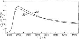
FIGURE 4.A.1 Predicted increase in atmospheric CO2 from A.D. 1900 to A.D. 3500: comparison of four-reservoir (4R) model and box diffusion (BD) model. The pattern of fossil-fuel consumption is as shown by the case n = 0.5 of Figure 4.8. The CO2 factor has the same meaning as for Figure 4.9.
model has thus been useful in indicating that a model with an analytical formulation distinctly different from that of the 6R model leads to a similar prediction of future CO2 levels, as in the case of predictions of the Suess effect. If either model is nearly correct, the prediction of atmospheric CO2 levels in the next 1500 years does not depend strongly on the assumptions regarding transport and storage of carbon in the subsurface water.
ADDITION MODELS
A variety of simple box models with more than two oceanic reservoirs and of continuous models with more parameters than the box diffusion model have been studied in connection with steady-state tracer distributions of subsurface ocean water. Few of these models, however, have been the basis for time-dependent studies, and most involve questionable ad hoc assumptions invoked to assign values to some of the model parameters when insufficient data are available. Stuiver (1973) and Veronis (1975) discuss some of the more interesting examples.
Since knowledge of subsurface ocean-water circulation stems largely from studies of the distributions of temperature and salinity, attempts have been made to combine studies of these measured properties with radiocarbon or other tracers having time-dependent properties. Simple box models have not been notably successful in explaining steady-state distributions of salinity and temperature. When small subsurface sources are neglected, both the 6R and the box diffusion models imply zero gradients in both quantities, suggesting difficulties in refining these models.
The simplest steady-state models that effectively use salinity and temperature data are advective-diffusive models. Typically these models assume tracer concentrations to be controlled by unspecified external processes at an upper and lower boundary between which constant vertical diffusion and upward advection prevail. The models have been most often applied to water at depths between 1000 and 4000 m, where the temperature and salinity vary almost exponentially with a vertical scale length of about 1000 m. If K and w denote, respectively, the vertical eddy-diffusion coefficient and upward velocity, the scale length directly reflects this ratio, i.e., K/w is equal to about 1000 m. If the radiocarbon is also considered, separate values for K and w can be computed. From a study of those few ocean stations where prebomb radiocarbon was measured, it is found that K is about 3000 m2 yr−1 [about 75 percent of the value preferred by Oeschger et al. (1975)]. Because the observed scale heights vary considerably from place to place, the significance of assuming constant values of K and w seems questionable. Also, the radiocarbon data used in these studies so far admit to considerable latitude in assigning values of K after the scale height is established. Thus the assumption of a constant value of K adopted by Oeschger et al. (1975) in their box diffusion model is not strongly supported by salinity and temperature data.
The vertical advective-diffusive models correctly reflect that cold salty water generally underlies warmer less salty water, and they explain in a reasonable way the distributions of salinity and temperature below 1000 m. These models have not, however, explained well the more complicated distributions lying between the surface layer and 1000 m in the region of the so-called intermediate water. As this water is of greater importance in predicting the uptake of industrial CO2 in the next few centuries than the deeper water, existing advective-diffusive models are not very adaptable to predicting the uptake of industrial CO2.
More complex two- and three-dimensional models have been proposed to explain subsurface oceanic tracer storage and transport, but these models also have mainly treated water below 1000 m. No model has explained well the more complicated distributions lying between the surface layer and 1000 m in the region of the intermediate water. As this water is of greater importance in predicting the uptake of industrial CO2 in the next few hundred years than is the deeper water, existing deep-water models are not very adaptable to predicting the uptake of industrial CO2. Until reliable dynamical models are developed for intermediate water, the simple box and box diffusion models are probably our best tools for predicting future atmospheric CO2 levels. Actually, the 6R and BD models may not be seriously deficient in this respect. The similarly small oceanic uptake of CO2 predicted by these models over the next 1500 years suggests that the choice of ocean model may not be crucial in establishing future CO2 levels.
With respect to predicting the uptake of CO2 by the land biota over the next few hundred years and longer, the choice of model is much more crucial. In Chapter 10, Revelle and Munk examine this problem in greater detail than previous investigators. In contrast to our exchange model, they postulate a cycling process in which carbon is transferred from the atmosphere to a carbon pool of living photosynthesizing material. This carbon is transferred to a pool of dead and detrital carbon including the wood of forest trees and thence back to the atmosphere without any reverse flow.
Revelle and Munk consider two principal cases. In one case, they assume for the photosynthesizing carbon pool a response to atmospheric CO2 similar to our model, and for the other carbon transfers, simple box model mechanisms. This first model predicts a damped oscillation in atmospheric CO2 level similar to a prediction of Eriksson and Welander (1956) (see Figure 10.1 in Chapter 10). For a pattern of production and total ultimate amount of industrial CO2 similar to that used in our model, their model predicts that atmospheric CO2 will fall from a peak concentration of 650 parts per million near A.D. 2100 to about 220 parts per million shortly before A.D. 2200. A century later, the concentration returns to near the preindustrial level of 290 ppm. Thus, in this case, with no limit on the biota pool size, the land biota carbon pool has taken up most of the industrial CO2 within a hundred years after its injection into the atmosphere.
If, on the other hand, Revelle and Munk assume that the
size of the photosynthesizing carbon pool remains fixed and that only the carbon pool of forest wood and detritus increases in size in response to higher atmospheric CO2 levels, they obtain a prediction that the biota carbon pool will increase by no more than about twice the amount of carbon in the preindustrial atmosphere (see Figure 10.3 in Chapter 10). This second model does not oscillate noticeably, nor does it predict an increase without limit in biota carbon for larger and larger inputs of industrial CO2.
Revelle and Munk also consider the effect on atmospheric CO2 of clearing of lands for agriculture and timber harvest. For the model with no limit on biota pool size, clearing has only a small influence on their predictions (see Figure 10.2 in Chapter 10). The model with a limit on the biota, which includes the effect of clearing, would probably be similarly insensitive to its exclusion, although this question was not investigated. Thus the most significant difference between the models almost certainly lies in the differing properties assigned to the photosynthesizing pool.
A possible limitation on the accuracy of these models is their simplified treatment of fluxes and storage times for short-, long-, and very long-cycled carbon species. Revelle and Munk have almost doubled the assumed quantity of organic carbon in the land biota by increasing the amount of soil humus, some of which may have very long cycling times. They have included this additional humus within a single box model reservoir that also includes short-cycled detrital carbon. The latter inclusion scarcely increases the assumed total amount of biotic carbon but approximately doubles the assumed flux to and from the detrital pool. This pool, with its single transfer time (of about 50 years), has a transfer function significantly different from that of a biota model with separate compartments for short-, long-, and very long-cycled carbon. This aggregating of fluxes and masses could result in an overestimate of biotic CO2 uptake.
On the other hand, the predicted CO2 uptake probably would be increased substantially by relaxing the requirement that the size of the photosynthesizing pool be constant. In the upper limit, with no restriction on pool size, the total land biota carbon pool is predicted eventually to take up all the industrial CO2 regardless of the amount. Little evidence exists from studies of plant communities to choose between such different models. Acceptance of a particular model seems therefore to depend mainly on the reasonableness of the prediction of biotic uptake of CO2. The work of determining the degree of uptake of CO2 that is reasonable probably must be done by ecologists, botanists, and soil scientists. When that work is done, the models can be adjusted to agree with their findings.
To prepare for this eventuality, we have investigated the result of assuming various amounts of biotic CO2 uptake using the 6R model with the biota growth factor linearly reduced to zero after A.D. 2000 over different time intervals. These predictions are based on quite arbitrary assumptions, but they reveal a feature of the carbon system that is probably only slightly model-dependent: for biotic uptake less than or of the order of that predicted by Revelle and Munk’s model with a limit on the biota, the sum of the uptake by the atmosphere and the biota is nearly the same regardless of the increase in biotic carbon. For example, with a cumulative increase in the biota in A.D. 2250 of 2.6 times the amount of preindustrial atmospheric CO2, the sum is only 3.7 percent greater than if the biota carbon pool grows negligibly.
Thus the predictions of atmospheric CO2 increase that we describe above in the main part of this chapter can be reduced by whatever the reader believes ought to be the uptake assigned to the land biota without seriously upsetting the model prediction in other respects. A similar option exists with respect to biota-limited models of the Revelle-Munk type, if assumed mechanisms controlling the photosynthesizing carbon pool are suitably varied.
REFERENCES TO APPENDIX 4.A
Bacastow, R. B., and C. D. Keeling (1973). Atmospheric carbon dioxide and radiocarbon in the natural carbon cycle: Changes from A.D. 1700 to 2070 as deduced from a geochemical model, in Carbon and the Biosphere, G. M. Woodwell and E. V. Pecan, eds., U.S. Atomic Energy Commission, pp. 86–135.
Craig, H. (1957). The natural distribution of radiocarbon and the exchange time of carbon dioxide between atmosphere and sea, Tellus 9, 1.
Ekdahl, C. A., and C. D. Keeling (1973). Atmospheric CO2 and radiocarbon in the natural carbon cycle: I. Quantitative deduction from the records at Mauna Loa Observatory and at the South Pole, in Carbon and the Biosphere, G. M. Woodwell and E. V. Pecan, eds., U.S. Atomic Energy Commission, pp. 51–85.
Eriksson, E. (1961). Natural reservoirs and their characteristics, Geofis. Internacional 1, 27.
Eriksson, E., and P. Welander (1956). On a mathematical model of the carbon cycle in nature, Tellus 8, 155.
Keeling, C. D. (1973). The carbon dioxide cycle: reservoir models to depict the exchange of atmospheric carbon dioxide with the oceans and land plants, in Chemistry of the Lower Atmosphere, S. I. Rasool, ed., Plenum Press, New York, pp. 251–329.
Machta, L. (1971). The role of the oceans and biosphere in the carbon dioxide cycle, in The Changing Chemistry of the Oceans, Proceedings of the Twentieth Nobel Symposium, D. Dryssen, ed., Wiley-Interscience, New York, pp. 121– 145.
Oeschger, H., U. Siegenthaler, U. Schotterer, and A. Gugelmann (1975). A box diffusion model to study the carbon dioxide exchange in nature, Tellus 27, 168.
Revelle, R., and H. E. Suess (1957). Carbon dioxide exchange between atmosphere and ocean, and the question of an increase of atmospheric CO2 during the past decades, Tellus 9, 18.
Stuiver, M. (1973). The 14C cycle and its implications for mixing rates in the oceans-atmosphere system, in Carbon and the Biosphere, G. M. Woodwell and E. V. Pecan, eds., U.S. Atomic Energy Commission, pp. 6–20.
Veronis, G. (1975). The role of models in tracer studies, in Numerical Models of Ocean Circulation, National Academy of Sciences, Washington, D.C., pp. 133– 146.
Von Arx, W. S. (1974). An Introduction to Physical Oceanography, Addison-Wesley, Reading, Mass.
Welander, P. (1959). On the frequency response of some different models describing the transient exchange of matter between the atmosphere and the sea, Tellus 11, 348.


