
10
Sexual Selection and Mating Systems
STEPHEN M. SHUSTER
Sexual selection is among the most powerful of all evolutionary forces. It occurs when individuals within one sex secure mates and produce offspring at the expense of other individuals within the same sex. Darwin was first to recognize the power of sexual selection to change male and female phenotypes, and, in noting that sexual selection is nonubiquitous, Darwin was also first to recognize the importance of mating systems—the “special circumstances” in which reproduction occurs within species. Analyses of mating systems since Darwin have emphasized either the genetic relationships between male and female mating elements, usually among plants, or the numbers of mates males and females may obtain, usually among animals. Combining these schemes yields a quantitative methodology that emphasizes measurement of the sex difference in the variance in relative fitness, as well as phenotypic and genetic correlations underlying reproductive traits that may arise among breeding pairs. Such information predicts the degree and direction of sexual dimorphism within species, it allows the classification of mating systems using existing genetic and life history data, and with information on the spatial and temporal distributions of fertilizations, it may also predict floral morphology in plants. Because this empirical framework identifies selective forces and genetic architectures responsible for observed male-female differences, it complements discoveries of nucleotide sequence variation and the expression of quantitative
Department of Biological Sciences, Northern Arizona University, Flagstaff, AZ 86011-5640.
traits. Moreover, because this methodology emphasizes the process of evolutionary change, it is easier to test and interpret than frameworks emphasizing parental investment in offspring and its presumed evolutionary outcomes.
Although sexual dimorphism and sexual differences were well known in his time, Charles Darwin (1859/1964, 1871, 1874) was first to recognize both their selective context as well as their evolutionary cause. Darwin’s initial observations about sexual selection focused mainly on the context in which sexual selection occurred, e.g., during combat involving “special weapons, confined to the male sex” (Darwin, 1859/1964, p. 88), as well as during female mate choice, wherein females “standing by as spectators, at last choose the most attractive partner” (Darwin, 1859/1964, p. 89). Darwin (1871, 1874) later identified the evolutionary process by which sexual selection occurs (see below), but his initial emphasis on context had already taken hold. Considerations of the context in which sexual selection occurs predominate to the present day [see reviews in Jones et al. (2002) and Shuster and Wade (2003)]. One goal of this chapter is to explain why it is time to deemphasize Darwin’s initial focus on context, and continue to develop Darwin’s later, more causeoriented evolutionary approach.
Darwin recognized too that sexual selection is nonubiquitous (Darwin, 1871, p. 208). His statement that “[i]n many cases, special circumstances tend to make the struggle between males particularly severe” demonstrates his intuitive grasp of mating system—the “special circumstances” in which reproduction occurs within individual species. Since Darwin, 2 emphases in mating systems have developed. The first is expressed in terms of the genetic relationships between males and females and is applied mainly to plants and domestic breeding designs. The second emphasis is expressed in terms of mate numbers per male or female, an approach usually applied to animals and mainly for typological classification. Contrary to Darwin’s description of the cause of sexual selection, evolutionary trends within animal mating systems are identified mainly in terms of energetic investment in individual offspring (Bateman, 1948; Williams, 1966; Trivers, 1972).
A second goal of this chapter, then, is to explain how disparate existing approaches to mating system analysis can be combined to yield a quantitative methodology that emphasizes measurement of the sex difference in the variance in relative fitness, as well as genetic correlations underlying reproductive traits arising from the spatial and temporal distributions of fertilizations. Such information predicts the degree and direction of sexual dimorphism within animal species, and may explain variation in floral
morphology among plants. This approach makes similar use of existing genetic, life history, and ecological data. It complements ongoing discoveries of nucleotide sequence variation and the expression of quantitative traits. It also may allow classification of plant and animal mating systems, using a common evolutionary framework.
TWO PERSPECTIVES ON SEXUAL SELECTION
Darwin (1859/1964) argued convincingly that male combat and female mate choice were the contexts in which sexual differences appeared. Yet Darwin observed too that sexual selection “depends, not on a struggle for existence, but on a struggle between males for possession of the females; the result is not death of the unsuccessful competitor, but few or no off-spring. Sexual selection is, therefore, less rigorous than natural selection” (p. 88). Darwin’s observations on the relative strength of sexual selection raise what can be considered a quantitative paradox (Shuster and Wade, 2003). How can sexual selection seem to be such a powerful evolutionary force, specifically responsible for causing the sexes to become distinct from one another, when sexual selection is less rigorous than natural selection? Stated differently, how can it be that sexual selection is strong enough to counter the opposing forces of male and female viability selection and still cause the sexes to become distinct (Shuster and Wade, 2003)?
Darwin provided an answer to this question when he devoted an entire volume to subject in 1871 (Darwin, 1871, 1874) and identified the specific cause of sexual selection: “if each male secures two or more females, many males cannot pair” (Darwin, 1874, p. 212). This relationship provided a conceptual solution to the quantitative paradox because it identified an evolutionary process responsible for causing the sexes to diverge. Darwin did not develop quantitative aspects of this particular hypothesis further himself but he was clearly aware of its power. Darwin likened the effect of this process to a bias in sex ratio, wherein particular males might disproportionately contribute to future generations, observations that set the stage for the development of the quantitative approaches now used to document sexual selection (Bateman, 1948; Wade, 1979; Wade and Arnold, 1980; Arnold and Wade, 1983; Arnold and Duvall, 1994; Jones et al., 2002; Shuster and Wade, 2003).
We can visualize the evolutionary process Darwin identified by noting, as Darwin did, that when sexual selection occurs, it creates two classes of males, those who mate and those who do not [cf. Wade (1979); Wade and Shuster (2004)]. If we let pS equal the fraction of males in the population who mate, and p0 = (1 −pS) equal the fraction of nonmating males, the average fitness of the mating males is pS(H), where H is the average number of mates per mating male. By the same principle, the average fit-
ness of the nonmating males is p0 (0). The average number of mates for all males equals the sex ratio, R = N♀/N♂, which can now be rewritten as
(1a)
wherein each term on the right side of the equation equals the fraction of males belonging to each mating class, multiplied by the average number of mates members of that class obtain. Because pS = (1 −p0), and because p0 (0) = 0, we can rewrite Eq. 1a as
(1b)
and if we allow the sex ratio, R, to equal 1, Eq. 1b can be expressed as
(1c)
Eq. 1c shows that when the value of H increases, the fraction of males without mates, p0, also must increase, a quantitative expression that captures what Darwin appears to have had in mind.
When females mate more than once, postcopulatory sexual selection via sperm competition is possible. This process can intensify sexual selection, but it need not (Shuster and Wade, 2003). Sperm competition intensifies sexual selection beyond that which occurs because of nonrandom mating only when a subset of the males who mate are also disproportionately successful in sperm competition. This condition increases the fraction of unsuccessful males overall because some of the males who successfully mate ultimately fail to sire offspring. In contrast, when mating success and fertilization success among males are uncorrelated, multiple mating by females always decreases the intensity of sexual selection because it increases the total number of males contributing to each generation. In general, because every offspring has one mother and one father (Fisher, 1930), when certain males fertilize ova disproportionately, other males must obtain fewer fertilizations. As Darwin suggested, differential success by some individuals must come at the expense of other individuals of the same sex. When this does not occur, sexual selection does not exist.
DARWIN ON MATING SYSTEMS
Darwin contributed two separate discussions on mating systems. The first concerned animal mating systems (Darwin, 1871). Here Darwin explained the diversity of male and female phenotypes attributable to the “special circumstances” in which sexual selection occurs (see above), confirming his understanding that sexual differences arose within this
context. Darwin’s second contribution on mating systems concerned those of plants. In The Different Forms of Flowers on Plants of the Same Species (Darwin, 1877a), Darwin detailed the various contrivances by which plants encourage or discourage cross-pollination. Although many plants appeared capable of selfing, Darwin observed (Darwin, 1877a, p. 266), “Various hermaphrodite plants have become heterostyled, and now exist under two or three forms and we may confidently believe that this has been effected in order that cross-fertilisation should be assured.” This statement confirms Darwin’s understanding that selfing was nonubiquitous among plants, and that floral differences arose within this context.
Like most of his contributions, Darwin’s original emphases have determined the research avenues pursued today. The two distinct emphases in current mating system research are almost certainly the result of Darwin’s distinction between plants and animals. The emphasis developed mainly for plants and domestic breeding designs is expressed in terms of the genetic relationships between males and females. The emphasis developed mainly for animals, following Darwin’s lead, is expressed in terms of mate numbers per male or per female.
PLANT MATING SYSTEMS
Darwin’s (1877a) approach to plant mating systems was mainly classificatory. He cataloged floral morphology according to its rich existing lexicon, and only secondarily developed hypotheses for why this variation might have evolved (Table 10.1). However, Darwin’s catalog seems intended to have been provocative. He described not only species with exclusive selfing, but also considered in careful, parallel detail the mechanisms by which selfing was prevented in certain species. Wright (1922) and Fisher (1941) later explored the population genetic consequences of various levels of selfing and outcrossing; Wright (1922) showed how selfing increased allelic autozygosity, and thus often resulted in inbreeding depression. Fisher (1941) showed how despite inbreeding’s potentially deleterious effects, selfing could increase in frequency when selfers contributed selfed as well as outcrossed seeds to each generation.
Consistent with these early emphases, recent research on plant mating systems has focused primarily on deviations from random mating (Barrett and Harder, 1996), and, with increasing resolution of genetic markers, population genetic approaches to plant mating systems and their theoretical foundations have become increasingly sophisticated. Selfing, self-incompatibility, dioecy and gynodioecy all appear to have evolved by remarkably simple means (Charlesworth and Charlesworth, 1978, 1987; Charlesworth, 2006). Obligate selfing and obligate outcrossing appear to persist as alternative stable states (Lande and Schemske, 1985),
TABLE 10.1 A Summary of Plant Mating Systems
|
General Category |
Fertilization Mode |
Definition |
Associated Terminology |
|
Perfect flowers |
Self-pollination |
Pollen fertilizes ovules on the same flower |
Autogamy, cleistogamy |
|
Cross-pollination |
Pollen fertilizes ovules on different flowers |
Chasmogamy |
|
|
Heterostyly |
Physical separation of style and stamen |
Distyly, tristyly |
|
|
Dichogamy |
Temporal separation of anther and stigma maturation |
Protandry, protogyny |
|
|
Self-incompatibility |
Pollen cannot fertilize ovules on the same plant |
Sporophytic, gametiphytic self-incompatibility |
|
|
Imperfect flowers |
Outcrossing |
Flowers are sex specific or exist as combinations of perfect and imperfect flowers |
Dioecy; androdioecy, gynodioecy |
whereas mixed mating systems seem constrained by the deleterious effects of inbreeding, despite frequent assumptions that a continuum can exist (see Schemske and Lande, 1985). Nevertheless, frequency-dependent and density-dependent processes in pollination transmission appear to have a powerful influence on whether selfing or outcrossing are stable within a given species (Holsinger, 1991). This result is consistent with observations that wind-pollinated plants conform to the predictions of Lande and Schemske (Lande and Schemske, 1985; Schemske and Lande, 1985), whereas animal-pollinated plants do not (Vogler and Kalisz, 2001), and furthermore, that patterns of floral morphology correspond to the relative amount of pollen available for export as well as to the density of conspecifics (Barrett and Harder, 1996).
Debate on the possibility that sexual selection can operate within plants (Willson and Burley, 1983; Cruzan et al., 1988; Lyons et al., 1989; Delph et al., 2002; Slogsmyr and Lankiinen, 2002; Shuster and Wade, 2003) has identified three primary contexts in which sexual selection might occur: (i) differential pollen transfer, (ii) differential pollen tube growth, and (iii) maternal control of seed set. However, although male and female fitness may vary within each of these contexts in plants, the extreme variance in male fitness seen in animals appears to be constrained by limited opportunities for pollen dispersal, by inconsistent success of particular pollen tubes among different stigmas, or by large within-individual variation in seed size and seed set, often due to pollen limitation (Ashman et al., 2004; Knight et al., 2005). Although male-male competition and female
preferences seem possible in plants, they do not lead to a sex difference in fitness variance comparable in magnitude to that of animals. Thus, despite the rigor of their theoretical foundations, and hints of similarities in mechanisms, studies of plant mating systems have remained conceptually divorced from those of animals.
ANIMAL MATING SYSTEMS
Perhaps because of Darwin’s observations on the greater physical modification of males and their greater eagerness to mate compared to females [“The exertion of some choice on the part of the female seems a law almost as general as the eagerness of the male” (Darwin, 1874, p. 217)] researchers in animal mating systems have primarily sought explanations for sexual differences in patterns of mating behavior, parental care, or in energetic allocations to progeny of each sex (Bateman, 1948; Williams, 1966; Trivers, 1972; Charnov, 1979). The resulting “parental investment theory” (Thornhill and Alcock, 1983) proposes that females, with their greater initial investment in offspring, are more inclined to provide parental care and that the small per-gamete investment in offspring by males predisposes males to abandon parental responsibilities in favor of additional copulations. The few, large ova of females are consistently identified as the limited resource for which males must compete to reproduce. Thus, the intensity of sexual selection on males is thought to depend on the degree to which females are rare.
Applying this reasoning, Emlen and Oring (1977) proposed two measures for understanding mating systems and for quantifying sexual selection, respectively. With the environmental potential for polygamy (EPP), these authors presumed to measure the degree to which the social and ecological environment allows males to monopolize females as mates. Emlen and Oring considered EPP highest when resources or females were spatially clumped and female receptivity was asynchronous, and lowest when resources were uniformly distributed and female receptivities were synchronous. This scheme has formed the basis for most considerations of animal mating system evolution [reviewed in Shuster and Wade (2003)], although EPP itself has proven difficult to define and quantify.
The second Emlen and Oring measure, the operational sex ratio (OSR), usually expressed as N♂(sexually mature)/N♀(sexually receptive) = OSR=RO, suggests that sexual selection results from competition among males for mates (Darwin, 1874). Thus, the OSR can be viewed as a reproductive competition coefficient among mating males. The greater the number of mature males relative to the number of receptive females, the greater the OSR and the stronger the presumed intensity of male-male competition for mates (Sutherland, 1985b; Ahnesjö et al., 2001).
Biases in OSR within populations are presumed to have significant evolutionary consequences, with effects ranging from both positive and negative influences on variance in mating success (Emlen, 1976; Shuster et al., 2001), to positive and negative influences on the intensity of sperm competition (Møller, 1989; Pen and Weissing, 1999) to the reversal of sex roles (Forsgren et al., 2004), to influences on mate selection and relative choosiness (Kokko and Monahagn, 2001), to influences on family sex ratio (Warner and Shine, 2007), aggressive behavior (Grant and Foam, 2002), female body temperature (Alsop et al., 2006), and declining population size (Stifetten and Dale, 2006). Methods for estimating OSR have used a wide range of modifications since their original identification, most notably including the ratio of male to female potential reproductive rates (PRR) (Clutton-Brock and Vincent, 1991).
These measures consider the effect on the intensity of sexual selection of particular receptive individuals at a particular time and in a particular place. The justification for this approach is that only certain individuals reproduce at any time, and including all males and females in such measurements could bias estimates of competition intensity. However, ignoring nonbreeding males, for example, omits those males whose numbers significantly increase the variance in male reproductive success, resulting in two kinds of errors in estimates of actual selection (Shuster and Wade, 2003). When nonmating individuals are ignored, a significant fraction of the among-group component of fitness variance goes unrecognized. This causes the mean fitness among mating individuals to be overestimated, and variance in fitness to be underestimated, respectively (Fig. 10.1). The stronger sexual selection becomes, the larger the possible error, because as fewer males mate, more of the male population is excluded from mating altogether. A similar problem exists for potential reproductive rates. Only a fraction of the actual population is considered in most measurements—those with the largest potential values. Under most circumstances, few if any individuals may ever achieve this rate.
A related difficulty involving field measurements of OSR compounds its unreliability as a metric for the intensity of sexual selection. Because instantaneous estimates of OSR during the breeding season fail to distinguish between males who mate and males who do not, such estimates tend to overestimate the intensity of sexual selection that exists over the entire breeding season (Shuster and Wade, 2003). To illustrate this point, consider two possible scenarios within a hypothetical breeding season in which 5 females mate with 5 males (Fig. 10.2). In this example, we assume that females mate once and their receptivity is maximally asynchronous; i.e., individual females mate sequentially across the breeding season. In Scenario 1, each female mates with the same male in a different jth interval (Fig. 10.2), whereas, in Scenario 2, each female mates in a different
![FIGURE 10.1 The effect of excluding nonmating males from estimates of average male mating success [cf. Shuster and Wade (2003)]. Shown are the outcomes for 100 randomly mating males and females when females are assumed to mate only once but males may mate repeatedly. m, mean mating success; Vm, variance in mating success when all males are included in parameter estimates (A) and when the zero class of males (hatched bars) is excluded from parameter estimates (B). The effect of omitting nonmating individuals from estimates of mating success tends to overestimate the average mating success and underestimate the variance in mating success for males.](/openbook/12692/xhtml/images/p20019ad4g199001.jpg)
FIGURE 10.1 The effect of excluding nonmating males from estimates of average male mating success [cf. Shuster and Wade (2003)]. Shown are the outcomes for 100 randomly mating males and females when females are assumed to mate only once but males may mate repeatedly. m, mean mating success; Vm, variance in mating success when all males are included in parameter estimates (A) and when the zero class of males (hatched bars) is excluded from parameter estimates (B). The effect of omitting nonmating individuals from estimates of mating success tends to overestimate the average mating success and underestimate the variance in mating success for males.
jth interval with a different male (Fig. 10.2). Although these scenarios are clearly distinct in their influence on sexual selection (one male mates with all of the females vs. each male mates with a different female), each case generates identical and thus indistinguishable instantaneous and overall values for OSR [RO(j) = N♂/N♀;(j) = 5; ΣRO(j) = 25; RO = N♂/N♀ = 5/5 = 1]. Note, too, that the sum of the instantaneous estimates of OSR, ΣRO(j), exceeds the overall estimate of OSR by 25-fold. There can be no doubt that the concept of OSR has stimulated considerable research. However, despite its conceptual utility, it is difficult to see how such an inconsistent measure can be responsible for the evolutionary power the operational sex ratio is now thought to possess.
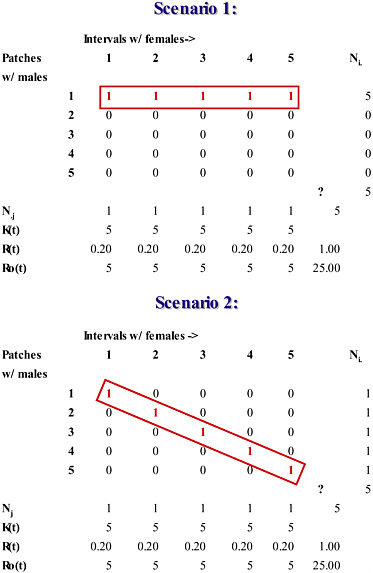
FIGURE 10.2 Instantaneous estimates of the operational sex ratio (OSR) during the breeding season fail to distinguish between males who mate and males who do not, and overestimate the intensity of sexual selection that exists over the entire breeding season. Shown are two scenarios illustrating a hypothetical breeding season in which 5 females mate with 5 males on territorial patches (rows). Within each jth interval of the breeding season (each column), the total number of receptive females, Nj, divided by the total number of males, Kt, equals Rt, the interval sex ratio, or the average number of females per male. The total number of males, Kt, divided by the total number of receptive females per interval, Nj equals the interval operational sex ratio, RO(t). In Scenario 1, each female mates with the same male in a different jth interval. In Scenario 2, each female mates in a different jth interval with a different male; each case generates identical and thus indistinguishable instantaneous and overall values for OSR (RO(j) = N♂/N♀(j) = 5; ΣRO(j) = 25; RO = N♂/N♀ = 5/5 = 1. Note that the sum of the instantaneous estimates of OSR, ΣRO(j), exceeds the overall estimate of OSR by 25-fold.
QUANTITATIVE ANALYSES OF MATING SYSTEMS
Covariance Methods
The most direct approach for investigating how sexual selection operates is to measure selection itself. Arnold and Duvall (1994) identified sexual selection gradients, which isolate the statistical relationship between male and female trait values and mating success relative to other components of selection. Using this method for pipefish (Syngnathus typhle), Jones et al. (2002) quantified the sex difference in “Bateman gradients,” in which females had a stronger positive association between mate numbers and fertility than males, and changes in sex ratio influenced the slopes of these relationships, as predicted by Emlen and Oring (1977). Bateman gradients are useful for studies of sexual selection because they quantify the slope of the regression of reproductive success (offspring) on mating success (mates that bear progeny). This standardized covariance between phenotype and fitness provides a direct measure of selection intensity on a particular trait, in this case, how mating success correlates with offspring numbers. Bateman gradients are part of the selection that acts on every sexually selected trait; thus they represent the final common path between sexually selected traits and fitness. When the gradient is zero, it shows that sexual selection is negligible and that selection in other contexts is likely to prevail.
Wade and Shuster (2005) used selection gradients as a means for understanding sex differences in eagerness to mate, by examining the covariance between average promiscuity and fitness for males and for females. This relationship provides a quantitative measure for “sexual conflict” as the sex difference in the sign of the covariance between numbers of matings and fitness. Such relationships show that when the sign of the covariance is negative, additional matings are favored in one sex but are selected against in the other, providing a simple statistical explanation for observed sex differences in eagerness to copulate not involving gametic differences [cf. Bateman (1948) and Trivers (1972)].
Again, because each offspring has a mother and a father (Fisher, 1930; Queller, 1997) and because each mating involves one male and one female (Wade and Shuster, 2005), this relationship shows too that it is impossible
for one sex to be more promiscuous on average than the other, as is often implied in extensions of parental investment theory (Thornhill and Alcock, 1983). The covariance approach also provides a means for predicting evolutionary trajectories if a genetic basis exists for particular traits associated with fitness. Under such circumstances genetic correlations may become established by the co-occurrence of particular male-female behaviors. For example, female tendencies to aggregate could become associated with male tendencies to defend breeding aggregations (Shuster and Wade, 1991, 2003; Wade and Shuster, 2005). Thus, in addition to the classic Fisherian runaway process, a wide range of correlated traits among the sexes could arise, beyond those involved in mate choice alone.
A related theoretical framework for understanding the evolution of correlated male traits as well as for considering how female traits may become enhanced or reduced as a result of interactions with males, is the covariance approach to social interactions (Frank, 1997; Moore et al., 1997; Roff, 1997; Wolf et al., 1999b). This methodology separates the effects of natural selection acting on traits possessed by focal individuals from the effects of social selection on these same traits, caused by interactions focal individuals may have with potential rivals or with potential mates themselves. The approach is applicable in the context of male-male interactions alone, as well as through female mate choice based on male phenotype, in the manner of Fisher’s (1930) runaway hypothesis of sexual selection.
The covariance approach provides a means for measuring the opportunity for social selection that exists whenever individual fitness varies as a result conspecific interactions (Wolf et al., 1999b). That is, it measures the maximum possible change in phenotype that is possible as a result of a single episode of social selection. This approach is conceptually similar to methods used to measure the opportunity for sexual selection (Wade, 1979; Wade and Arnold, 1980; Shuster and Wade, 2003) (see below), and it is analogous to contextual models of multilevel selection (Goodnight et al., 1992; Whitham et al., 2003), in which the effects of group structure or membership on individual fitness are each identified and quantified using partial regression models.
A Sex Difference in the Opportunity for Selection
The above methods rely on the experimenter’s ability to identify specific traits that are associated with fitness variance. Another method for identifying the intensity of sexual selection that does not require such specificity compares the fitness of parents who successfully breed, with the fitness of the population before reproduction occurs. Crow (1958, 1962) showed that this comparison provides an estimate of the opportunity for selection, an empirical estimate of the maximum possible change in a
phenotypic distribution as a result of one episode of selection. The opportunity for selection, I, is equivalent to the variance in fitness, VW, divided by the squared average in fitness, W2, and equals the variance in relative fitness, Vw (Wade, 1979; Shuster and Wade, 2003).
When paternity data are available, the sex difference in the opportunity for selection is estimated by calculating the opportunity for selection separately for each sex. Here, the value of I for each sex is expressed as the ratio of the variance in offspring numbers, VO, to the squared average in offspring numbers, O2, among the members of each sex, or, I♂ = VO♂/ O♂2 and I♀ = VO♀/O♀2 (Shuster and Wade, 2003; Wade and Shuster, 2005; Shuster, 2008) Because each offspring has a mother and a father (Fisher, 1930), I♂ and I♀ are linked through the sex ratio and mean fitness in terms of offspring numbers, which also must be equal for both sexes (Wade and Shuster, 2005). The sex difference in the variance in relative fitness, ∆I = (I♂ − I♀), when considered in this way may be positive, negative, or zero (Shuster, 2008). The value of ∆I determines whether and to what degree the sexes will diverge in character because fitness variance is proportional to selection intensity.
When ∆I > 0, sexual selection modifies males and ∆I = Imates, the opportunity for sexual selection as described initially by Wade (1979). When ∆I < 0, the variance in offspring numbers is greater for females than it is for males and sexual selection modifies females, as is expected to occur when sex roles are reversed (Shuster, 2008). When ∆I = 0, there is no sexual selection in either sex or sexual selection is equally strong in both sexes, a condition that can lead to extreme sexual dimorphism because sexual selection is likely to favor distinct, divergent evolutionary trajectories for males and for females (Shuster and Wade, 2003). The opportunity for selection identifies the maximum possible change in phenotype because it contains all of the variance in fitness, selected as well as random. Some authors have criticized the usefulness of I because chance alone can influence variance mating success as well as offspring numbers (Sutherland, 1985b; Hubbell and Johnson, 1987). Indeed, bad things can happen to good genes and vice versa (Shuster and Wade, 2003). However, because mate numbers and offspring numbers are the currency by which I is measured, the outcomes of chance on mating success and fertilization success are already incorporated into these estimates of selection opportunities. Crow (1958, 1962) identified I as the opportunity for selection for good reason. Because random processes can diminish the effectiveness of selection, I estimates an upper limit on the response to selection.
This approach is distinct from that currently used by parental investment theory (Bateman, 1948; Williams, 1966; Trivers, 1972; Thornhill and Alcock, 1983). According to this latter framework, males and females are defined by differences in energetic investment in gametes. However, a
causal scheme based on sex differences in parental investment fails to explain the details of male parental care within and among even closely related taxa. Among syngnathid fish, for example, stickleback males (Gasterosteus aculeatus) build benthic nests, use their bright red undersides to attract mates, and care for multiple clutches of eggs. In this species, male care enhances a male’s ability to mate (Baker J, et al., 1998; Ah-King et al., 2005), whereas, in seahorses (Hippocampus spp.), males and females form pairs, males receive the eggs of a single female into their brood pouch and provide exclusive parental care to young that eliminates further male mating opportunities (Vincent and Sadler, 1995). It is unclear how such diversity can possibly evolve if initial parental investment is the cause of sex differences in phenotype and parental care.
When paternity data are unavailable, it is still possible to estimate opportunities for selection by exploiting the multiplicative properties of male and female fitness (Shuster and Wade, 2003). This approach makes use of the fact that the average male fitness equals the average number of mates per male, m, multiplied by the average number of offspring per female, O. Thus, the total variance in offspring numbers for males, VO♂, can be estimated in terms of the average number of mates per male and the average number of offspring per female. As in a standard ANOVA problem, the total variance in male fitness can be partitioned into the sum of two components: (i) the average variance in offspring numbers for males within the classes of males who sire progeny, and (ii) the variance in the average number of progeny sired by males among these same mating categories (Shuster and Wade, 2003; Wade and Shuster, 2004; Shuster, 2008).
Spatial and Temporal Distribution of Matings
The above approach for estimating the intensity of sexual selection relies on the availability of information on the mean and variance in clutch sizes and numbers in females, and the mean and variance in mate numbers among males. When such information is unavailable, an alternative approach for measuring sexual selection builds on the conceptual framework of Emlen and Oring (1977) and examines the spatial and temporal distribution of matings. Although the Emlen-Oring estimates of the environmental potential for polygamy (EPP) and the operational sex ratio (OSR) have proven unsatisfying from an empirical standpoint as described above, two methods by Shuster and Wade (2003) capture these authors’ unique insight that spatial and temporal variation in the availability of mates provides crucial information on whether multiple mating by particular individuals can occur.
How does each method work? The first method involves construction of a matrix whose rows represent resource patches or other territories con-
taining males and whose columns represent intervals during the breeding season during which females may be receptive (cf. Figs. 10.3 and 10.4; rows may also represent territorial females in sex-role-reversed species). As described in Shuster and Wade (2003) the duration of each interval equals the average duration of receptivity among all females. The cells of the matrix may contain zeros or larger numbers identifying the number of mates males obtain within each interval. If multiple males inseminate the same female, these numbers may also represent the fraction of the total fertilizations with a given female that a male obtains, providing a specific means for considering the effects of postcopulatory sexual selection. The more precise paternity data are, the more detailed such analyses can be, and fractions of clutches instead of individual matings can be substituted into the matrix.
Although algebraically complex, partitioning the total variance in mate numbers among males into spatial and temporal components is in practice straightforward (Fig. 10.3) (Shuster and Wade, 2003), amounting to an ANOVA problem in which the total numbers of matings (Fig. 10.3, upper left rectangle) are partitioned into the within- and among-
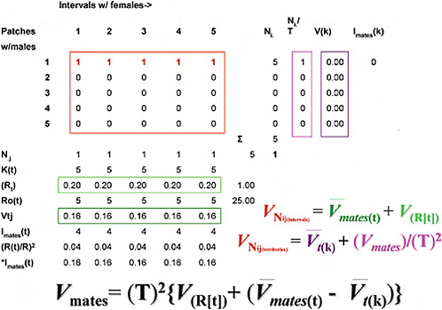
FIGURE 10.3 Methods for partitioning the total variance in mate numbers among males into spatial and temporal components (explanation in Spatial and Temporal Distribution of Matings).
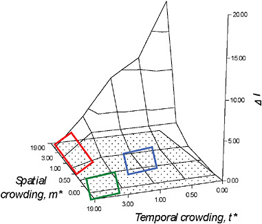
FIGURE 10.4 The ΔI surface. As explained in detail in Shuster and Wade (2003), simultaneous consideration of the mean spatial crowding of matings, m*, and the mean temporal crowding of matings, t*, provides opportunities to visualize how spatial and temporal distributions of matings influence the opportunity for sexual selection, ΔI, as well as the dynamic nature of mating system evolution. Changes in mating system character occur as a result of modifications in the spatial and temporal distribution of matings. When m* is low and t* is high, males are likely to seek out, remain with, and provide parental care for isolated, synchronously receptive females, forming persistent pairs (lower left rectangle); when m* is moderate to high, t* is high, males are expected to defend individual females, but breeding is expected to occur in large aggregations or mass matings (upper left rectangle). Polygamy is likely when m* and the mean temporal crowding of matings, t* are both moderate (right rectangle).
male components of mating success obtained in space and in time. As in ANOVA, we identify two components of variance: that arising within the classes of mating males and that arising among all males, mating as well as nonmating. To begin, note that within each jth interval of the breeding season (each column), the total number of receptive females, Nj, divided by the total number of males, Kt, equals Rt, the interval sex ratio, or the average number of females mated by each male within the jth interval (upper horizontal rectangle, Fig. 10.3). The average of the squared number of females mated by males within each jth interval, ΣNj2/Kt, minus the squared interval sex ratio, Rt2, equals Vtj, the variance in mates per
male, per jth interval (lower horizontal rectangle, Fig. 10.3). The temporal distribution of matings then equals the variance in male mating success across all j intervals, VNij(intervals), which equals the average of the variances in mates per male per jth interval, Vmates(t) (= ΣVtj/T), plus the variance of the average sex ratio across all j intervals, ![]() , or
, or
(2a)
Within each ith male territory (row), the total number of receptive females, Ni, divided by the total number of intervals containing at least one female, T, equals Ni/T, the number of females mated by the male in the ith territory, averaged across all T intervals (left vertical rectangle, Fig. 10.3). The average of the squared number of females mated by each male within the ith territiory per Tth interval, ΣNi2/T, minus the squared average number of mated females across all T intervals, (Ni/T)2, equals V(k), the variance in mate number across all T intervals for the ith territorial male (right vertical rectangle, Fig. 10.3). The spatial distribution of matings then equals the variance in male mating success across all i territories, VNij(territories), which equals the average of the variances in mate number across all T intervals per ith territorial male, ![]() , plus the variance of the average number of females mated by the ith male across all T intervals, (Vmates)/(T)2, or,
, plus the variance of the average number of females mated by the ith male across all T intervals, (Vmates)/(T)2, or,
(2b)
Shuster and Wade (2003) showed that these two estimates of the variance in mate numbers among males can be combined so that the total variance in male mating success across all j intervals (Eq. 2a) and i territories (Eq. 2b) equals the total variance in male mating success, Vmates, and that
(2c)
Noting that the average mating success for all males equals the sex ratio, R = N♀/N♂, Shuster and Wade also showed that when Vmates (cf. Eq. 2c) is divided by R2, this ratio equals the opportunity for sexual selection, Imates (= ΔI when I♂ > I♂), which can be rewritten as
(3)
Eq. 3 shows how the total opportunity for sexual selection, determined from the temporal distribution of matings among spatially distinct territorial males, can be partitioned into three components: (i) Isex ratio, the opportunity for sexual selection caused by temporal variation in the sex
ratio (this is what the OSR appears to have been designed to measure, but does not because it overestimates the intensity of sexual selection within intervals in which females are abundant); (ii) *Imates(t), the weighted opportunity for sexual selection caused by temporal variation in the availability of females (this value may be small or large depending on whether females are synchronous or asynchronous in their receptivities, and is weighted by the number of females that appear in each interval, with larger numbers of females per interval contributing the largest effects); and (iii) *Imates(k), the weighted opportunity for sexual selection caused by spatial variation in the availability of females, which may be small or large depending on whether females are spatially dispersed or spatially clumped. Note that *Imates(k) erodes *Imates(t) because the latter term is an estimate of the variance in mate number within individual territorial males. Increases in the variance in relative fitness within males tend to decrease the variance in relative fitness that occurs among males.
Spatial and Temporal Crowding of Sexual Receptivity
The above method considers the total variation in mating success as separate opportunities for selection arising from (i) variation in sex ratio across the breeding season, (ii) the temporal availability of mates, and (iii) the spatial availability of mates. In effect, this scheme captures the elements of mating system variation identified by Emlen and Oring (1977) (i.e., EPP and OSR) and expresses them in terms of their relative influences on the intensity of sexual selection. This approach does not require data on parentage (although such information can make this approach more precise), but it does require specific information on which males mate with which females. When only the spatial and/or temporal distributions of sexually receptive individuals are available, yet another method for estimating ΔI involves calculating the mean spatial crowding, m* and the mean temporal crowding, t*, of such individuals (Lloyd, 1967; Wade, 1995; Shuster and Wade, 2003).
The mean crowding approach for estimating ΔI requires simply that the spatial and temporal distributions of matings be identified. In most cases, the spatiotemporal distribution of receptive females provides this information. For example, the mean crowding of receptive females (matings) on resources defended by males, m*, can be expressed as
(4)
where m equals the average number of receptive females per resource patch, and Vm is the variance around that average. In this context, m* represents the number of other females the average female experiences
on her resource patch. When females are maximally dispersed among patches, m* approaches zero, whereas when females tend to aggregate on particular patches, m* increases.
Similarly, when the breeding season is divided into intervals whose width equals the average duration of female receptivity, the mean temporal crowding of female receptivity over the breeding season, t*, can be expressed as
(5)
where t equals the average number of receptive females per interval and Vt equals the variance around that average. In this context, t* represents the number of other receptive females the average receptive female experiences when she becomes sexually receptive. When female receptivity is maximally asynchronous within the breeding season, t* approaches zero, whereas when female receptivities overlap within a single interval, the value of t* becomes large.
Although values of m* and t* can each estimate the opportunity for sexual selection, ΔI (= Imates when I♂ > I♀), in most cases it is necessary to measure both values because the effects spatial and temporal crowding of females may have on male fertilization success are distinct. Whereas the relationship between m* and ΔI is proportional, i.e., at mmax one or a few males could defend and mate with all of the females in the population, the relationship of between t* and ΔI is reciprocal, i.e., at tmax, the ability of one or a few males to mate with multiple females is reduced. The combined effects of m* and t* on sexual selection generate a surface (Fig. 10.4) that bears striking resemblance to Emlen and Oring’s (1977) diagram of possible values for the environmental potential for polygamy. However, unlike these authors’ conceptual model, the ΔI surface provides actual estimates of selection intensity from empirical estimates of female spatial and temporal distributions.
Common Ground for Plant and Animal Mating Systems
As explained in detail in Shuster and Wade (2003), simultaneous consideration of m* and t* provides opportunities to visualize the dynamic nature of mating system evolution. Unlike typological classifications, this framework predicts that even slight modifications in the spatial and temporal distribution of matings can cause rapid changes in mating system character. Furthermore, when similar values of m* and t* exist among taxonomically diverse species, the mating systems of these species should begin to converge. For example, when m* is low and t* is high, males are likely to seek out, remain with, and provide parental care for isolated,
synchronously receptive females, forming what can be called “persistent pairs” (Shuster and Wade, 2003) (Fig. 10.4). Examples of such mating systems may occur in sponge shrimp (Spongocola spp.) (Saito and Konishi, 1999), which enter the bodies of spatially dispersed glass sponges (Hexactinellidae) as larvae, and later differentiate into male-female pairs that remain imprisoned within the sponge for life. Similar spatial dispersion and temporal synchrony in reproductive activity appear to characterize the mating systems of desert isopods (Baker M, et al., 1998) and solitary sandpipers (Oring, 1973).
If females become more spatially aggregated, m* is moderate to high, t* is high, males are expected to defend individual females, but breeding is expected to occur in large aggregations, forming what can be called “mass mating” (Shuster and Wade, 2003) (Fig. 10.4) Examples of such mating systems may occur in explosively breeding frogs (Wells, 1979), grunion (Thomson and Muench, 1977), or simultaneously spawning cnidarians (Kruger and Schleyer, 1998) and, although seldom discussed in this way, perhaps in dioecious wind-pollinated plants such as junipers (Thomas et al., 2007).
Polygamy appears to occur when the mean spatial crowding of matings, m*, and the mean temporal crowding of matings, t* are both moderate (Shuster and Wade, 2003) (Fig. 10.4). Here, not only do males and females have approximately similar variance in mating success and so tend to show little sexual dimorphism, but when individuals are limited in their mobility or are restricted to patchy habitats, they may also be simultaneously or sequentially hermaphroditic. Examples of this mating system are found in caridean and pandalid shrimp (Charnov, 1979; Bauer, 2000), as well as in barnacles (Hoch, 2008), and terrestrial slugs (Reise et al., 2007). Again, although seldom discussed with the breeding systems of animals, similar mating systems may also exist in plants with perfect flowers, or that show tendencies toward heterostyly and dichogamy (Darwin, 1877a).
Considerations of mean spatial and temporal crowding of matings provide insight into the character of animal mating systems, but this approach may also be useful for plants (Fig. 10.5). A possible scheme for variation of this sort might place self-fertilizing (cleistogamous) plants in circumstances in which both m* and t* are low, i.e., spatially dispersed and temporally asynchronous, conditions that could lead to extreme pollen limitation and favor individuals who self. In contrast, outcrossing species could be most commonly represented in circumstances in which ecological conditions favor higher densities of breeding individuals and relative synchrony of breeding phenology. Wind-pollinated plants may typically occur when natural selection favors synchronous breeding, regardless of their spatial distribution, whereas animal-pollinated plants may be most
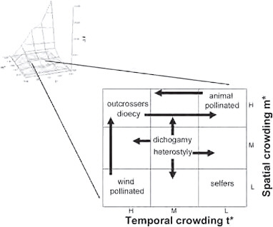
FIGURE 10.5 The location on the ΔI surface in which plant mating systems and animal mating systems may be considered within the same empirical framework. Such conditions exist in the center of the distribution, at approximately the same conditions in which polygamy is favored in animals and where sexual selection is relatively weak.
common when plants are spatially aggregated, regardless of whether flowering is temporally clumped or aggregated (Fig. 10.5).
Heterostylous plants may be represented at intermediate values of m* and t* but show greater representation at lower spatial density and temporal asynchrony, as such conditions could favor the long-distance, asynchronous arrival of pollinators, whereas dichogamous plants may also be represented at intermediate values of m* and t* but show greater representation at higher spatial densities and synchronous flowering, as such conditions could favor temporal specialization via male or female function. Dioecy could be favored when pollen limitation seldom occurs, as when plants are relatively clumped in space and temporally synchronous in their flowering, but could also exist when spatially clumped flowers open asynchronously and allow plants to attract pollinators over long durations and gain considerable fitness through pollen.
Sexual selection is considered relatively weak among plants because of approximately equivalent fitness variance within each sex (Shuster and Wade, 2003). Such conditions seem most likely to occur when the values of m* and t* are moderate. The location on the ΔI surface in which such conditions exist for animals is the center of this distribution, where polyg-
amy is favored and sexual selection also tends to be relatively weak (Fig. 10.5). Thus, the most productive place to begin investigation of how the spatial and temporal distributions of fertilizations are similar in plants and animals may be with these polygamous species. Few data are now available that could test the generality of this hypothesis. However, sufficient anecdotal information exists to justify efforts by researchers to close the conceptual and empirical gap between studies of plant and animal mating systems. As if to invite collaborative research, the population genetic tools, both theoretical and empirical, that characterize research in plant mating systems are less well developed for animals, while the spatiotemporal data and quantitative genetic methods for measuring selection that characterize research in animal mating systems are less well developed for plants. Each discipline has much to offer the other and much exciting work remains to be done.
ACKNOWLEDGMENTS
I thank Michael J. Wade for his fundamental role in developing the ideas presented in this manuscript, John Avise and Francisco Ayala for organizing In the Light of Evolution III, and 2 anonymous reviewers for their comments on an earlier draft of this manuscript. This work was supported by National Science Foundation Grants NSF FIBR-0425908 and DBI-0552644.


