Below are the first 10 and last 10 pages of uncorrected machine-read text (when available) of this chapter, followed by the top 30 algorithmically extracted key phrases from the chapter as a whole.
Intended to provide our own search engines and external engines with highly rich, chapter-representative searchable text on the opening pages of each chapter. Because it is UNCORRECTED material, please consider the following text as a useful but insufficient proxy for the authoritative book pages.

Do not use for reproduction, copying, pasting, or reading; exclusively for search engines.

OCR for page 193
Appendix B Technical Discussion of Atmospheric Transport Mechanisms Once an air pollutant is released into the atmosphere, chemical, microphysical, and meteorological factors determine how it is distributed. The location of air pollution sources with respect to local, regional, and global air circulation patterns influences how efficiently pollutants are transported and dispersed. The winds transport air both horizontally and vertically. Vertical transport is important when considering long-range pol- lutant transport because pollutants distributed to higher altitudes usually encounter stronger winds that provide rapid transport to distant locations. Atmospheric stability, controlled by how temperature varies with height, determines whether vertical transport will be slow or rapid. After emission, pollutants may undergo chemical transformation, be subjected to depletion processes such as particle scavenging and dry or wet deposition, or mix into the atmosphere to become a component of the background concentration. This appendix provides a general description of the atmosphere and a syn- opsis of air circulation and weather patterns that influence the distribution of air pollutants. VERTICAL STRUCTURE Pollutant transport occurs in the lowest two layers of the atmosphere— the troposphere and stratosphere. Most weather phenomena that affect pol- lutant transport occur in the troposphere, which extends from the surface to ~ 18 km in the tropics and ~ 8 km near the poles (Figure B.1). The tropo- pause is the zone of transition between the troposphere and stratosphere. The height of the tropopause does not uniformly decrease in the poleward 

OCR for page 193
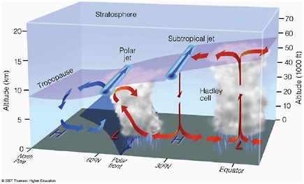
 APPENDIX B FIGURE B.1 Cross-section from the equator to the North Pole showing three cir- culation cells, the tropopause, and the polar and subtropical jet streams. B-1.eps SOURCE: Ahrens, 2007. bitmap image direction. Instead, there are two climatologically occurring breaks in each hemisphere, one containing the subtropical jet stream (near 30° N), and the other containing the polar jet stream (near 45° N). These jet streams are not stagnant in location, but shift with season, moving closer to the equator in winter and more poleward during summer. The jet streams are important distributors of air pollutants for two rea- sons. They create major areas of air exchange between the troposphere and stratosphere. And the strong winds of the jet stream can rapidly transport pollutants. For example, if one assumes an average wind speed of 35 m s–1 (~ 70 kt) at 40° latitude, an eastward-moving air parcel will circumnavigate the globe in only 10 days. The stratosphere, which extends to ~ 50 km, has regions of strong winds, but virtually no turbulent mixing except for occasional overshooting thunderstorms, certain types of lightning, and occasional thin clouds. The atmosphere’s vertical temperature profile plays the dominant role in controlling whether and how quickly an air pollutant will be dispersed upward from its point of emission. The change of temperature with height or lapse rate is used to quantify vertical temperature profiles. The average midlatitude tropospheric temperature lapse rate is 6.5°C km–1, with actual values constantly changing in both time and three-dimensional space. Large lapse rates (like those near the surface on a sunny day) are associated with atmospheric instability, which promotes turbulence. Conversely, small lapse rates near the surface (as would occur on a cold, windless night) denote

OCR for page 193
 APPENDIX B stability that suppresses vertical motion. Layers containing temperature inversions (a negative lapse rate) are very stable, greatly inhibiting vertical transport and promoting the accumulation of pollutants. Inversions in the troposphere can occur when the surface is colder than the overlying air and in subsiding air, which occurs in regions of high pressure. The stratosphere is a permanently stable region, with a near zero lapse rate between 11 and 20 km and increasingly negative (stable) rates above. As a result of this stability pollutants injected into the stratosphere tend to remain there for much longer periods than in the troposphere. An important characteristic of free tropospheric air movement is that air parcels experiencing no exchange of heat energy conserve their poten- tial temperature and thus move along surfaces of constant potential tem- perature (isentropic surfaces). Exceptions are regions of cloud cover where radiative processes and water vapor phase changes can be major sources or sinks of heat. In addition, air parcels in the surface boundary layer undergo temperature changes due to exchanges of radiation with Earth’s surface. Isentropic surfaces slope upward toward the north, with isentropic values increasing vertically (Figure B.2). As a result poleward moving air conserv- ing its potential temperature tends to ascend, while equatorward-moving air tends to sink. This concept has applications for pollution transport into the Arctic (Stohl et al., 2006; Law and Stohl, 2007). Specifically, pollution- laden parcels beginning at low altitudes and heading north that conserve their potential temperature will ascend to the middle troposphere. Con- versely, for low-level parcels to remain near the surface during northward excursions, they either must be very cold initially or undergo considerable loss of heat due to passing over ice-covered surfaces, especially during the long polar winter seasons. Northern Eurasia is sufficiently cold that its pollutants can be transported quasi-horizontally to the Arctic, making it a major source of Arctic pollution during winter. GLOBAL CIRCULATION FEATURES Global circulation patterns are driven by the nonuniform distribu- tion of incoming solar energy, with the greatest energy being received near the equator. The general circulation can be considered the multiyear seasonal average of the daily winds. The smaller, shorter-lived circulations described later are removed, leaving the largest, longest-lasting wind pat- terns. The flow in the tropical troposphere (±0°-30°) is dominated by the Hadley Circulation Cell (Figure B.3) which contains rising air along the Intertropical Convergence Zone (ITCZ). This ascent produces a band of enhanced clouds and precipitation. Subsiding air and relatively clear skies occur at the poleward boundary of the Hadley Cell. A component of this sinking air moves southward to replace the air that has ascended up and

OCR for page 193
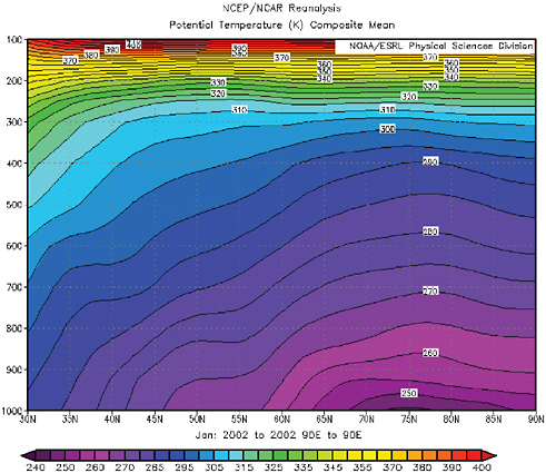
 APPENDIX B FIGURE B.2 Cross-section of mean potential temperature (K) from 30° N to the North Pole. Note that the isentropes 2.eps B- slope upward toward the pole. Air parcels move along isentropic surfaces when no heatage is added or subtracted. bitmap im energy away from the equator. Thus, the meridional flow is equatorward at low levels and poleward above. The middle latitudes (30°-60°) are dominated by transient cyclones (low-pressure areas) and anticyclones (high-pressure areas), especially during the winter. In the long term mean the region is characterized by sinking air near 30° and rising air at its northern bound- ary (~ 60°), corresponding to the location of the polar front. This region sometimes is denoted the Ferrell Cell (not depicted in Figure B.3). The polar troposphere (60°-90°) is dominated by rising air near 60° and sinking air over the poles, sometimes denoted the Polar Cell. The simplified view of the global circulation described above becomes more complex when the effects of continents and oceans are included. Global sea-level pressure patterns and surface winds for January and July are shown in Figure B.4. Focusing on the Northern Hemisphere, the Janu-

OCR for page 193
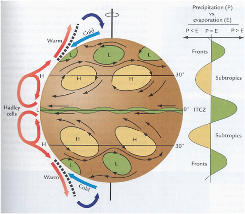
 APPENDIX B FIGURE B.3 An idealized representation of Earth’s general circulation. B-3.eps SOURCE: Ahrens, 2007. bitmap image ary pattern (Figure B.4a) is dominated by high-pressure air masses with clockwise circulating winds over the relatively cold Eurasian and North American continents. The Bermuda and Pacific high-pressure regions are evident but weak. Conversely, the Icelandic and Aleutian Lows represent the average of transient synoptic-scale low-pressure systems that form near the east coasts of Asia and North America and then move eastward, reach- ing maximum intensity near the location of lowest pressure in the figure. Air circulates counterclockwise around these lows. One should note the ITCZ that extends around the globe just south of the equator; it represents the confluence of the northeasterly trade winds (Northern Hemisphere) with the southeasterly trades (Southern Hemisphere) and is an important area of interhemispheric transport. Global circulations during the Northern Hemisphere summer (Fig- ure B.4b) are quite different from those during winter. Low pressure, not high pressure, now dominates the continents, producing the seasonal wind

OCR for page 193
 APPENDIX B A B B-4a.eps bitmap image FIGURE B.4 Climatological mean sea-level pressure and winds for (a) January and (b) July. The Intertropical Convergence Zone (ITCZ) is shown by the red line near the equator. B-4b.eps SOURCE: Ahrens, 2007. bitmap image

OCR for page 193
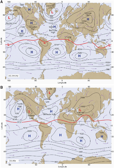
 APPENDIX B reversal called the monsoon. In Asia, for example, there is offshore flow during the winter but onshore flow during summer. The quasi-permanent Bermuda and Pacific high-pressure regions are larger and better defined dur- ing summer than winter. Their southern extents produce the northeasterly trade winds, which combined with their Southern Hemisphere counterpart, produce the ITCZ that now is located north of the equator. The Icelandic and Aleutian storm tracks are poorly defined because their constituent synoptic-scale transient lows are much weaker during summer. Global flow patterns in the middle and upper troposphere (Figure B.5) are simpler than those near the surface. Prominent features are easterly flow in the deep tropics, clockwise flow around the semipermanent high-pressure regions in the subtropics, and circumpolar cyclonic flow. The prevailing westerlies, which contain north to south undulations cover a major por- tion of the Northern Hemisphere. The westerlies are stronger during winter than summer. The following points summarize the role of global circulations in pro- ducing long-range transport. 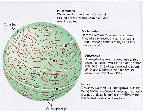FIGURE B.5 Climatological flow patterns in the middle troposphere. SOURCE: Anderson and Strahler, 2008. Reproduced with permission of John Wiley B-5.eps and Sons Inc. bitmap image was tipped 3 degrees clockwise and chopped off on right

OCR for page 193
00 APPENDIX B • Winds in the middle-latitude troposphere are mostly from the west (zonal flow), causing most intercontinental transport to be from west to east. • The north-south (meridional) component of the wind in the middle and upper troposphere usually is much weaker than the zonal component. The two components can have similar magnitudes near the surface. • Wind speeds generally are stronger during winter than summer, causing more rapid transport during the winter months. The jet streams in the upper troposphere are regions of strongest winds. • Wind speeds in the troposphere generally increase with altitude. Thus, the vertical motion experienced by air parcels is vitally important since pollutants that are transported from near the surface to higher alti- tudes usually will be horizontally transported the most rapidly. Areas of rising air tend to be smaller and shorter lived than areas of subsidence, which generally cover larger areas and persist longer. SYNOPTIC SYSTEMS Synoptic circulation features have sizes of ~ 1,000-2,000 km and life- times of several days to a week. Transient middle-latitude cyclones (lows) and anticyclones (highs) are prime examples of these circulations. Anti- cyclones generally are regions of tranquil weather with sinking air that leads to relatively cloud-free skies and stable conditions that suppress mixing and tend to trap pollutants. Their light winds also reduce horizontal transport. Anticyclones with little forward motion allow these stagnating conditions to persist over days or even weeks. Low-pressure areas are important regions of strong horizontal and vertical pollution transport. Locations of cyclone initiation (cyclogenesis) and their subsequent storm tracks are important in determining the routes of long-range pollution transport. Once a cyclone begins to form it is “steered” by upper tropospheric flow patterns, generally toward the east. Important areas of cyclogenesis are located over eastern Asia and the west- ern Pacific Ocean, as well as the east coast of North America. Cyclones forming in these areas are important mechanisms for transporting pollut- ants from the east coasts of both Asia and North America (Merrill and Moody, 1996; Cooper et al., 2002a,b; Stohl et al., 2002). Another preferred region of cyclogenesis is downwind of major mountain ranges such as the Rocky Mountains or the Alps. It is noteworthy that Europe and western Asia are not major regions of cyclone formation or transit. The instantaneous flow around cyclones in the northern hemisphere is counterclockwise. However, if one considers three dimensional trajectories with respect to a moving cyclone, three specific pathways (or airstreams) often are identified—the warm and cold conveyor belts and the dry intru-

OCR for page 193
0 APPENDIX B sion (Figure B.6) (Browning and Monk, 1982; Browning and Roberts, 1994; Bader, 1995; Carlson, 1998). The warm conveyor belt (WCB) is a major transporter of pollutants (Stohl et al., 2002; Eckhardt et al., 2004). It begins near the surface in advance of the cyclone’s cold front (i.e., its warm sector). If the cyclone forms sufficiently offshore, relatively clean maritime air is transported by the WCB. If the low forms closer to land, surface-based pollutants from the heavily industrialized regions of eastern Asia and eastern North America are transported by WCBs. The pollution- laden air rises slowly at first but more quickly as it approaches the cyclone’s warm front. The thunderstorms that sometimes are embedded within the WCB can produce localized regions of much more rapid ascent (Kiley and Fuelberg, 2006). When the air has ascended to the middle troposphere, it begins to move eastward and become part of the background westerly flow. By the end of the conveyor the air typically has reached the altitude of the tropopause (~ 9 km). The transport time from the boundary layer near the east coast of the United States to the European free troposphere typically is three to four days (Stohl et al., 2002; Eckhardt et al., 2004), but can be as short as two days if the jet stream is particularly strong (Stohl et al., 2003). Due to the greater distance for transpacific transport, an extra day or two may be required to move pollution from East Asia to North America, again depending on the strength of the jet stream (Cooper et al., 2004). In some cases a second cyclone may be involved. As its name implies the cold conveyor belt is located completely within the cold sector of the cyclone (Figure B.6). The low-level air flows toward the west along the north (cold side) of the surface warm frontal position. During part of this route, the WCB is overhead. As cold air approaches the center of the cyclone the air begins to ascend into the middle troposphere while making a clockwise loop, eventually reversing direction and combin- ing with the WCB in the upper troposphere. The role of the cold conveyor belt in transporting pollutants aloft has received relatively little attention. The dry air intrusion (DI) of a middle-latitude cyclone originates in the upper troposphere and lower stratosphere (Figure B.6). It is located on the poleward side of the cyclone and descends into the middle to lower tropo- sphere. The DI is characterized by subsidence and often by regions of much lower tropopause height (tropopause folds) that are related to the jet stream aloft. Thus, the DI can transport upper tropospheric or stratospheric air into the middle or lower troposphere. Some authors have described a cold, dry post-cold-frontal airstream in the middle to lower troposphere beneath the DI and behind the surface cold front (Cooper et al., 2001). It is noteworthy that air masses also can be transported long distances without being lifted (i.e., the air and its pollutants remain in the lower troposphere). This generally occurs in the absence of transient synoptic systems that would contain mechanisms for ascent (e.g., the WCB). Arctic

OCR for page 193
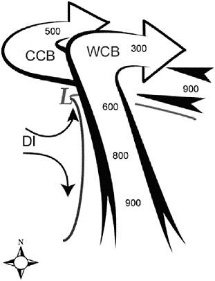
0 APPENDIX B FIGURE B.6 Airstream configuration as depicted in the classic cyclone model (adapted from Carlson, 1998). Airstreams are the warm conveyor belt (WCB), cold conveyor belt (CCB), and dry intrusion (DI). Numbers indicate the approximate pressure altitudes (hPa) of the airstreams. The surface low-pressure center is indi- cated with an “L”. The lines extending south and east of the low-pressure center Figure B-6 indicate the surface cold front and warm front, respectively. SOURCE: Kiley and Fuelberg, 2006.Bitmapped haze (Barrie, 1986) has been attributed to this low-level transport (Klonecki et al., 2003; Stohl, 2006; Law and Stohl, 2007). It also has been observed downwind of North America over the North Atlantic Ocean (Neuman et al., 2006), the Azores (Owen et al., 2006), and Europe (Li et al., 2002; Guerova et al., 2006). Similar phenomena have been observed over the North Pacific Ocean (Liang et al., 2004; Holzer et al., 2005) and the Indian Ocean during the winter monsoon (Ramanathan et al., 2001). MESOSCALE SYSTEMS Mesoscale weather systems have typical sizes of a few hundred kilometers and lifetimes ranging from a few hours to a day. Important examples

OCR for page 193
0 APPENDIX B associated with pollutant transport are thunderstorms, land and sea cir- culations, and mountain and valley breezes. These circulations either can be superimposed on the larger scale transient systems or they can occur alone. Thunderstorms occur frequently over many parts of the world, rang- ing from isolated cells to organized clusters called mesoscale convective systems (MCSs). The bases of thunderstorms typically are ~ 1.5 km above the surface, while the tops of nonsevere isolated cells or disorganized clusters extend to near the local tropopause. Updrafts and downdrafts generally are less than 10 m s–1. The structure and life cycle of a typi- cal nonsevere thunderstorm is shown in Figure B.7. These storms can rapidly move boundary layer pollutants to the upper troposphere where they can be transported great distances by the stronger horizontal winds aloft (Dickerson et al., 1987; Lelieveld and Crutzen, 1994). Conversely, the downdrafts that occur during the mature and dissipating stages of a storm transport upper tropospheric air to the surface. Nonsevere storms can be associated with cyclones and frontal systems or be embedded within homogeneous synoptic air masses. A prime example is Florida and sur- rounding states, which experience almost daily thunderstorms during the warm season. Examples of severe convection include supercells, multicell complexes, and squall lines. Doswell (2001) presents an excellent summary of severe convective storms. 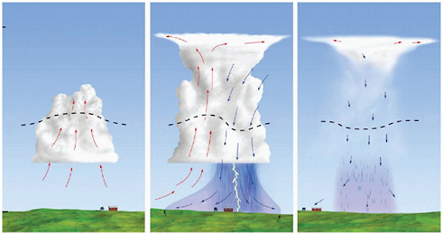These storms have three important characteristics that FIGURE B.7 Life cycle of a typical nonsevere thunderstorm. Updrafts are shown as B-7.eps red arrows and downdrafts by blue arrows. The storm initially (left panel) contains only updrafts but contains only bitmap image dissipation (right panel). downdrafts during SOURCE: Ahrens, 2007.

OCR for page 193
0 APPENDIX B relate to atmospheric transport. First, their updrafts are much stronger than their nonsevere counterparts, often reaching 40 m s–1, allowing the storms to overshoot the tropopause and extend several kilometers into the strato- sphere. These strong updrafts can transport boundary layer air to the upper troposphere or lower stratosphere on the order of minutes, compared with hours or days for synoptic systems. This is an important consideration for short-lived chemical species. Second, the structure of severe storms differs from that of nonsevere storms. For example, the cross-section through a mature squall in Figure B.8 reveals a rear inflow jet that transports mid- level air downward and toward the surface. Supercell storms and multicell systems (not shown) have somewhat different structures. Severe storms generally have a long lifetime, often lasting 12 h or more. Thus, the storms can move long distances during their lifetimes and produce strong vertical transport over a large area for an extended time. A newly discovered type of convection is associated with wildfires. These pyroconvection events can transport large quantities of aerosols and gases into the upper troposphere and lower stratosphere (Damoah et al., 2006; Fromm et al., 2000, 2005; Jost et al., 2004; Luderer et al., 2007). In summary, deep convection is a very efficient transporter of bound- ary layer air to the free troposphere (Dickerson et al., 1987; Park et al., 2001). Cotton et al. (1995) estimated an annual flux of 4.95 × 1019 kg of boundary layer air by cloud systems (including extratropical cyclones), which represents a venting of the entire boundary layer about 90 times a year. 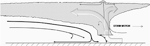Calculations for the central United States suggest that nearly 50 per- cent of boundary layer CO is transported to the free troposphere by deep convection during summer (Thompson et al., 1994), while a typical middle latitude squall line was found to transport of 9.9 × 103 tons of CO out of FIGURE B.8 Cross section perpendicular to a squall line (adapted from Houze et al., 1989). Large hollow arrows identify epsascending front to rear inflow (left) B-8. the and core updraft transporting air to the cloud top and forward anvil (right). Black arrows represent the rear inflow jet supporting e cold pool generation directly bitmap imag the below the core updraft.

OCR for page 193
0 APPENDIX B the boundary layer over an 8 h simulation period, 3.89 × 104 t past 500 hPa, and 2.88 × 104 t of CO above 300 hPa (Halland et al., 2009). Sea and land breezes are important sources of mesoscale transport in all three dimensions. They are examples of mesoscale diurnally varying thermal circulations that form due to temperature contrasts between the land and adjacent ocean (Simpson, 1994). During the warm part of the day, the land surface is warmer than the ocean, producing onshore surface flow (the sea breeze). The extent of inland penetration is greatly influenced by the direction of the prevailing larger scale wind. The flow above the sea breeze is reversed (offshore winds) to complete the circulation cell, with the depth of the complete circulation usually confined to the lowest 3 km of the atmosphere. The leading edge of the advancing low level sea breeze is a region of strong ascent that often produces thunderstorms in humid regions of the world. At night the temperature gradient reverses, causing offshore flow near the surface (the land breeze) and onshore wind aloft. The land breeze usually is much weaker than its daytime counterpart. Sea and land breezes can transport coastal emissions offshore during the day and onshore during the night. Mountain and valley circulations also are diurnally varying mesoscale thermal circulations. In this case the horizontal temperature gradient is due to altitude differences. During the day, the mountains act as an elevated heat source, causing air and its pollutants to rise up the side of the sloping terrain. Under summertime fair weather conditions three times the volume of the valley can be lofted into the free troposphere each day (Henne et al., 2004). If conditions are favorable, the ascent can lead to thunderstorm development along the mountain tops. At higher altitudes away from the mountains the air sinks into the surrounding valleys. At night the horizontal temperature gradi- ent reverses, producing downslope flow into the nearby valley that is assisted by gravity. This can lead to an accumulation of pollutants in the valley. Without mountain and valley circulations mountain ranges could block the horizontal transport of pollutants. If the daytime upslope flow is suf- ficiently strong, the polluted air can rise up and over the mountains and be transported away from its source by the stronger winds aloft. Mexico City is a prime example of where terrain-induced circulations strongly affect pollu- tion concentrations (Fast et al., 2007; Lei et al., 2007; De Foy et al., 2008). MICROSCALE MOTIONS Turbulence is the prime example of microscale circulations. Turbulence is important in pollution transport because it can thoroughly mix the air and its pollutants. A well-mixed layer is characterized by vertically uniform concentrations of pollutants, water vapor, and potential temperature. The depth of the mixed layer is denoted the planetary boundary layer (PBL).

OCR for page 193
0 APPENDIX B There are two major categories of surface-based turbulence. Mechani- cally-induced turbulence occurs when the prevailing horizontal wind is dis- rupted by a rough surface. Thermally-induced turbulence occurs when the temperature lapse rate is large, producing a relatively unstable surface layer and causing the unevenly heated surface to produce pockets of ascent and descent. Since over land both the prevailing wind speed and temperature lapse rate typically are strongest during the day, mixing generally is stronger during the day than the night. Therefore, the height of the mixed layer also varies diurnally (Stull, 1988). There is much less diurnal variation over water. Boundary layer turbulence appears to be the major source of vertical transport in parts of Asia. Dickerson et al. (2007) found that the warm- sector PBL air ahead of a cold front was highly polluted while in the free troposphere, concentrations of trace gases and aerosols were less but still well above background. They concluded that dry convection appears to dominate vertical transport, with warm conveyor belts first coming into play as the cyclonic systems move off the coast. As the PBL collapses with the onset of evening, pollutants that were transported aloft by turbulence remain, forming a residual layer (Stull, 1988) that is decoupled from the surface and thereby experiences stronger wind speeds than air within the PBL (Angevine et al. 1996). Most turbulence in the free troposphere (above the PBL) is produced by an optimum combination of temperature lapse rate and the degree to which the prevailing winds vary with height (wind shear). Although the forcing mechanisms differ, the effect is the same—turbulence in the free atmosphere thoroughly mixes the air. TRACKING AIR PARCELS—TRAJECTORY APPROACHES It often is important to determine the source of air pollution at a spe- cific location or where pollution from a given source will be located in the future. The basic concept is simple if one has an accurate four-dimensional (x,y,z,t) representation of temperature and wind. One simply uses the data to advect air parcels backward or forward over increments of time. Accu- rately applying this concept is very difficult because of the myriad types and scales of processes that affect transport. The isentropic and kinematic methods are the most widely used pro- cedures for calculating trajectories. The isentropic method assumes that an air parcel conserves its potential temperature during the computational period. Thus, the parcel is advected on its sloping isentropic surface by the horizontal winds. The vertical component of the wind is not needed in these calculations since parcels are assumed to change altitude because of the slope of the isentropic surface. The isentropic assumption generally is very good in the stratosphere for periods of a week or longer since there are no surface radiative processes and few clouds. Nonetheless, radiative processes

OCR for page 193
0 APPENDIX B increasingly violate the isentropic assumption over time. The isentropic assumption is violated much more quickly in the troposphere, where it is usually not the preferred methodology for calculating trajectories. The kinematic method utilizes the three dimensional wind components at an initial location to advect air parcels over an interval of time. Once at the new location and time the wind components at that location and time are used to advect the parcel. The process continues for the desired time period. As with isentropic trajectories the wind data are from numerical meteorological models whose grid spacing typically varies from ~ 50 to 150 km for global data, down to a few km for regional models. The models typically contain approximately 50 levels in the vertical, often with closer spacing near the surface and near tropopause level. An example of 10-day backward trajectories is shown in Figure B.9. Particle dispersion models are an advanced version of the trajec - tory concept. They have been widely used in relatively recent transport studies. A well-known example is the FLEXPART model (Stohl et al., 2005). 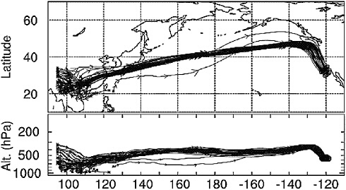Dispersion models require three-dimensional wind components from either coupled or off-line meteorological models, and may contain modules that seek to incorporate the effects of convection and other sub-grid-scale motions that are not adequately represented by the input meteorological FIGURE B.9 Cluster of 10-day backward trajectories arriving just offshore of Southern California and initiating over9.eps B- Southeast Asia. The upper panel is a plan view; the lower panel is longitude versus image (hPa). The trajectories arrive at bitmap altitude 0000 UTC March 12, 1999. SOURCE: Adapted from Martin et al. (2003).

OCR for page 193
0 APPENDIX B data (e.g., Forster et al., 2007). In addition, each particle that is released at a source can be assigned a mass that is related to the rate of emission. Thus, maps showing future concentrations of a species can be produced. An example of a FLEXPART run is given in Figure B.10. Trajectories and particle dispersion models require a perfect depiction of the atmosphere at every time step to be totally accurate. This is a corol- lary to the famous statement that every time a butterfly flaps its wings, its motion will ultimately affect the weather (Lorenz, 1963). Unfortunately, however, vast areas of Earth have sparse or even no surface-based observa- tions. Although satellite remote sensing reduces the problem, some synoptic systems still are inadequately resolved, with smaller systems being diag- nosed even less accurately. As an example, individual thunderstorms and their updrafts and downdrafts will not be resolved by a global atmospheric model having a horizontal resolution of 50 km, or even a regional model at a resolution of 10 km. Instead, the models will utilize parameterization schemes to diagnose the composite effects of the storms at the scale of the model. Parameterization schemes also are used to simulate the effects of boundary layer processes, radiative effects, and other processes. Inadequate numerical techniques to compute the trajectories are another factor limiting the accuracy of trajectories. As a result of our inability to completely describe all atmospheric motions, trajectories (and weather forecasts) deteriorate with time. 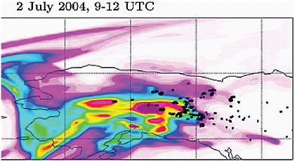The exact rate of deterioration is very difficult to quantify since it depends on FIGURE B.10 Total column of CO tracer from the forward FLEXPART simulation shown for July 2, 2004, 0900–1200 UTC. Black dots show MODIS fire detections B-10.eps on the respective day. bitmap image SOURCE: Adapted from Stohl et al. (2006).

OCR for page 193
0 APPENDIX B the types of weather phenomena that are occurring and how well they are detected and parameterized. INTERCONTINENTAL POLLUTION TRANSPORT Figure 1.2 in Chapter 1 depicts the major pathways of pollution trans- port in the Northern Hemisphere, considering first the transpacific trans- port from Asia toward North America. Modeling studies indicate that the transport occurs year round (Liang et al., 2004), but is strongest during spring when three to five Asian plumes affect the boundary layer of the west coast of the United States between February and May (Yienger et al., 2000). This is due to the frequency and structure of the eastward-moving middle-latitude cyclones and the exact paths they take. Strong Asian plumes have been observed by aircraft over the eastern North Pacific Ocean (Heald et al., 2003; Nowak et al., 2004) and the west coast of the United States (Jaffe et al., 1999, 2003a; Jaeglé et al., 2003; Cooper et al., 2004). Most of the plumes were associated with lifting of East Asian pollutants by the WCBs of middle-latitude cyclones. As noted previously, there is considerable stratospheric-tropospheric exchange and general subsidence to the rear of the cyclones. As the cyclones decay along the west coast of North America, the plumes dissipate and become part of the hemispheric pollution back- ground. Some Asian plumes have remained sufficiently intact that they have been detected over Europe (Stohl et al., 2007). Most of the North American export toward the east also is associated with middle-latitude cyclones and their associated WCBs (Figure 1.1 in Chapter 1). Evidence of North American pollution has been observed in the European free troposphere (Stohl, 1999; Stohl et al., 2003; Trickl et al., 2003) and at high-altitude surface sites in the Alps (Huntrieser et al., 2005). Weak effects of North American pollution have been detected at Mace Head, Ireland (Derwent et al., 2007). Forest fires over Alaska and Canada have produced greater enhancements of low-level concentrations at Mace Head (Forster et al., 2001). There is no major cyclonic storm track between Europe and Asia (Fig- ure B.4), and few studies have examined the transport of European pollu- tion to Asia (Newell and Evans, 2000; Pochanart et al., 2003; Duncan and Bey, 2004; Wild et al., 2004a). Newell and Evans (2000) estimated that on an annual basis, only 24% of the air parcels arriving over Central Asia had passed over Europe, with 4% originating in the European PBL. European pollution also has been detected over eastern Siberia (Pochanart et al., 2003), Japan (Wild et al., 2004), and North Africa (Lelieveld et al., 2002; Stohl et al., 2002). Instead, European emissions are exported at relatively low altitudes and strongly affect the Arctic (Stohl et al., 2002; Duncan and Bey, 2004).

OCR for page 193
0 APPENDIX B SUMMARY The sections above indicate that many meteorological phenomena on a variety of spatial and temporal scales transport surface pollutants out of the boundary layer and into the free troposphere, including thunderstorms, turbulence, sea breezes, and the warm conveyor belts of cyclones.1 Donnel et al. (2001) found that advection was the most important mechanism for transporting tracer to the free troposphere; and the addition of upright convection and turbulent mixing increased the amount by up to 24 percent, with convection transporting the tracer to heights of 5 km. They concluded that the convection and turbulent mixing were not linearly additive pro- cesses, emphasizing the importance of representing all such processes in meteorological modeling studies. More generally, the long-range intercontinental transport of pollutants can be considered a two-step process. First, the pollutants must be trans- ported vertically out of the boundary layer where winds are relatively light and into the free troposphere where winds are stronger, especially near the jet stream. Once in the free troposphere the pollutants are transported quasi-horizontally by larger wind systems such as the prevailing westerlies. The strength of the winds determines how rapidly the transport will occur, and there can be considerable mixing with stratospheric air above the troposphere. Many middle-latitude low-pressure areas form near the highly industri- alized east coast of Asia. Their WCBs can carry the pollutants aloft where they are transported quasi-horizontally toward the west coast of North America. If convection occurs near the low-pressure area, the upward trans- port occurs much more rapidly. The low pressure development is episodic, occurring approximately every four days during the winter and spring but less often during the warm season. Therefore, the pollution tends to traverse the North Pacific in elongated bursts or plumes before becoming part of the background concentration at even greater distances from their Asian source. The heavily populated east coast of the United States also is a region of enhanced low pressure development. Similar to that described for eastern Asia, the WCBs, and possibly convection associated with the developing lows, vertically transport the pollutants out of the polluted boundary layer where they are carried eastward toward Europe. Transport from Europe to Asia occurs mainly in the lower troposphere because Europe is not a major region of low pressure development. However, when deep convec- 1 In contrast, there is relatively little quantitative information comparing the relative roles of gravitational settling, scavenging by precipitation, and other processes that transport pol- lutants back down to the surface. This is an area that requires additional research.

OCR for page 193
 APPENDIX B tion occurs, low level pollution can be quickly transported aloft into the westerlies. The transient low pressure systems described above are middle latitude phenomena. Transport from the Sahara to the far southeastern United States occurs at lower latitudes and is due to quasi-permanent subtropical high pressure located over the Atlantic Ocean (Bermuda and Azores Highs). The clockwise flow around these systems produces easterly winds that pro- vide the westward transport. The Arctic lower troposphere is isolated from the rest of the atmosphere by its very cold air, i.e., the Arctic front. However, the front is not zonally symmetric, and can extend to 40°N over Eurasia during January. Thus, northern Eurasia is the major source of Arctic pollution during winter. Air from further south can be transported to the Arctic, but only in the middle and upper troposphere. During summer, the transport is from the North Atlantic Ocean, across the high Arctic, and toward the North Pacific.

OCR for page 193