
Overview of Climate Changes and Illustrative Impacts
The following section provides an overview of a number of climate changes and impacts that can now be identified and estimated at different levels of warming. Highlighted in bold are the key impacts followed by supporting details.
CHANGES IN RAINFALL AND STREAMFLOW
Increases of precipitation in high latitudes and drying of the already semi-arid regions at lower latitudes are projected with increasing global warming, with seasonal changes in several regions expected to be about 5-10% per degree of warming. However, patterns of precipitation change show much larger variability across models than patterns of temperature. The basic large-scale pattern and magnitude of precipitation responses across the tropics, subtropics, and mid-latitude and high-latitude regions can be understood largely as the result of increasing water vapor in the atmosphere; these are broadly consistent with observed trends and physical understanding, and represent a very robust prediction across models. Precipitation in many of the world’s monsoon regions is expected to increase during the rainy season. Precipitation associated with mid-latitude storms is also expected to increase. For some areas, particularly those near transitions between regions that become wetter and those that become drier, model disagreement is large. The continental U.S. region straddles changes that are both positive (over the northernmost areas) and negative (over the southwest areas) changes in both annual and Dec-Jan-Feb average precipitation. A large portion of the contiguous 48 U.S. states is in a transition zone where future rainfall changes cannot be projected with confidence at present. Models agree in projecting increases in precipitation on the order of 5-10% per degree C of warming in high latitudes in all seasons, including over Alaska,
and they also project drying in the dry season in the south and southwest United States and Mexico (see Figure O.1). {4.2}
Streamflow Changes
Widespread changes in streamflow are expected in a warmer world, with many regions experiencing changes of the order of 5-15% per degree of warming. Streamflow is a key index of the availability of freshwater, a quantity that is essential for human and natural systems. Changes in streamflow depend upon both evaporation (and hence warming) as well as precipitation. In regions where decreases in precipitation are predicted, these decreases usually will be accompanied by larger decreases in streamflow.
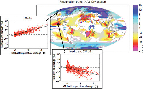
FIGURE O.1 Estimated changes in precipitation per degree of global warming in the three driest consecutive months at each grid point from a multi-model analysis using 22 models (relative to 1900-1950 as the baseline period). White is used where fewer than 16 of 22 models agree on the sign of the change. One ensemble member from each model is averaged over the dry season and decadally in several indicated regions including southwestern North America and Alaska, as shown in the inset plots. Adapted from Solomon et al. (2009), with additional inset panel for Alaska (courtesy R. Knutti) provided using the same datasets and methods as in that work. {4.2}
Streamflow is expected to decrease in many temperate river basins as global temperature increases. The greatest decreases are expected in areas that are currently arid or semi-arid. Most models project decreases in the southwest United States, while slight increases are projected in the northeast and northwest. There is strong agreement among models that runoff in the Arctic and other high-latitude areas, including Alaska, will increase. The greatest decreases per degree within the United States are projected for the Rio Grande Basin (about 12% per degree) and increases of about 9% per degree are expected in Alaska; see Figure O.2. Thus, warming of a few degrees can be expected to lead to large perturbations to water resources, especially in the southwestern and southern parts of the United States, many of which are already facing water resources challenges due to growing population and environmental issues. {5.3}
CHANGES IN EXTREME TEMPERATURE, PRECIPITATION, AND CLIMATE DYNAMICS
Temperature Extremes
Extreme temperatures are expected to increase in a warmer world. For example, for about 3ºC of global warming, 9 out of 10 Northern Hemisphere summers are projected to be “exceptionally warm” in nearly all land areas, and every summer is projected to be “exceptionally warm” in nearly all land areas for about 4ºC, where an “exceptionally warm” summer is defined as one that is warmer than all but about 1 of the 20 summers in the last decades of the 20th century. A complete review of the many studies evaluating changes in extremes in various regions is beyond the scope of the present study. Here we use as an illustrative example the effect of warming on seasonal extremes, based on a simple shift in the distribution of temperatures, using pattern scaling. Some studies have indicated the possibility that the variance of the distribution of temperature will increase, especially in regions that are projected to become drier (e.g., the Mediterranean basin), further enhancing the chances of extreme seasonal temperatures beyond that estimated here (see Figure O.3). {4.5}
Extreme Precipitation
Extreme precipitateon (heaviest 15% of daily rainfall) is likely to increase by about 3-10% per degree C as the atmospheric water vapor content increases in a warming climate, with changes likely to be greater
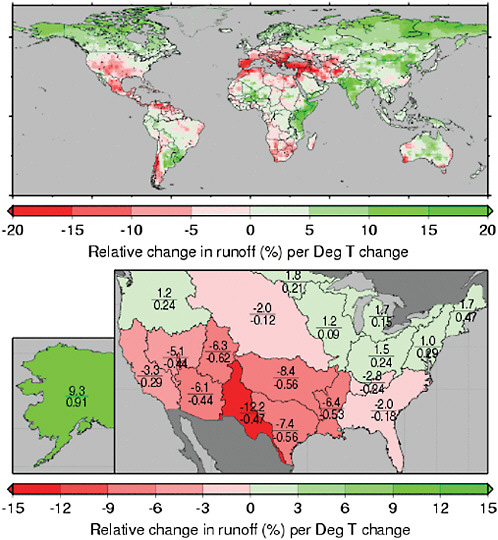
FIGURE O.2 Median runoff sensitivities (per degree of global warming) relative to 1971-2000 over 68 model pairs. Each pair consisted of an average over A2, A1B, and B1 global emissions scenarios of one IPCC Assessment Report 4 (AR4) GCM model’s output, derived from 30-year runoff averages centered on the years for which the global average temperature increases were 1.0ºC, 1.5ºC, and 2.0ºC, minus the 30-year model average runoff for 1971-2000, divided by the global temperature change. This analysis was performed for 23 models for 1.0ºC and 1.5ºC increases, and 22 models for a 2.0ºC increase. Results are shown as averages over GCM grid cells (upper plot) or U.S. hydrological regions (lower plot). The notation a/b in each river basin denotes the mean change in percent (a), and the agreement among models (b); expressed as the fraction with positive changes minus the fraction with negative changes (FPN); see also Table 5.3. Table 5.3 contains standard errors and consistency across models, as indicated by FPN.
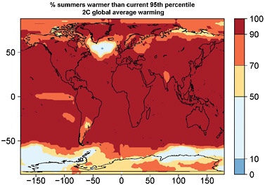
FIGURE O.3 Percentage of northern summers (June-July-August) warmer than the warmest 95th percentile (1 in 20) for 1971-2000, for 2ºC global average warming above the level of 1971-2000, or about 3ºC total warming since pre-industrial times, from an analysis of the multi-model CMIP3 (Coupled Model Intercomparison Project phase 3) ensemble. {4.5}
in the tropics than in the extratropics (this sensitivity may decrease somewhat as the warming progresses). While changes in precipitation extremes could lead to changes in flood frequency, the linkage between precipitation changes and flooding will be modulated by interactions between precipitation characteristics and river basin hydrology, the nature of which are not yet well understood. {4.6}
Hurricanes and Typhoons
Averaged over the tropics as a whole, the number of tropical cyclones is expected to decrease slightly or remain essentially unchanged. Models suggest that the average intensity of tropical cyclones (as measured by the wind speed) is likely to increase roughly by 1-4% per degree C global warming, or by 3-12% per degree C for the cube of this wind speed, often taken as a rough measure of the destructive potential of storm winds. For the North Atlantic, the changes in hurricane statistics are more uncertain than the global values, depending in large part on the spatial structure of the warming of the tropical oceans, and not just on the local warming in the Atlantic. Recent models project future changes in the number of Atlantic hurricanes ranging
from –25% to +25% per degree C of global warming; thus, the sign of future changes in number of storms is uncertain. {4.3}
Ocean Circulation
The Meridional Overturning Circulation (MOC) in the Atlantic Ocean is expected to slow down in the 21st century due to warming associated with increased greenhouse gases and associated increased ocean stratification. As a result, warming in the northern North Atlantic Ocean and surrounding maritime regions is expected to be smaller than other oceanic regions. Changes in fisheries and marine ecosystems could also result from a MOC slow-down, but these impacts are poorly understood. {5.8}
CHANGES IN ICE, SNOW, AND FROZEN GROUND
Sea Ice
Arctic and Antarctic sea ice extent and volume are projected to decrease over the 21st century if greenhouse gas emissions continue to increase. Models project a clearly defined linear relationship between annual Arctic sea ice area decreases and global averaged surface air temperature. According to an analysis of an ensemble of models, annually averaged Arctic sea ice area reductions of about 15% are expected per degree C of global average warming (see Figure O.4). Greater reductions are expected for summer
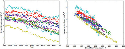
FIGURE O.4 Changes in annually averaged Arctic sea ice extent versus time from 13 CMIP3 models (left). The same information is plotted versus global mean temperature in the righthand panel. {4.7}
compared to winter. Figure O.4 illustrates that the retreat of Arctic sea ice is more compact when plotted versus global mean temperature rather than time, and this aids the understanding of the effect of stabilization at various target levels. Published studies of the range of the date when late summer Arctic sea ice is expected to disappear range from 2037 to beyond 2100. Models suggest that late summer Arctic sea ice decreases rapidly if warming exceeds about 2ºC. By the end of the 21st century (global warming of about 3-5ºC relative to pre-industrial conditions) an ice-free Arctic ocean in late summer is predicted by most models. In the decades after 2100, two models suggest that ice-free conditions may occur in winter if polar temperatures reach 13ºC above present-day values. In the Antarctic, models predict a loss in ice cover ranging from 10-50% in winter and 33-100% in summer for a warming of about 1.7-4.4ºC. The relationship between annual average sea ice area and the global average temperature suggests that ice recovery may occur if temperatures decrease. {4.7}
Snow Cover and Snowpack
Current trends in snow cover over the Northern Hemisphere suggest that the snow cover season has shortened and spring melt is occurring earlier compared to the past 50-100 years. Modelled changes in Northern Hemisphere snow cover are similar to the observations. Future decreases are consistent across the models and may reach –18% by 2090 (or a global warming of about 2-3ºC). Snowpack has decreased over much of western North America since 1925, and this decrease has been linked to increasing temperatures over the West. While regional responses to the warmer surface temperatures may vary, the overall response suggests a significantly shorter snow season, smaller areal coverage, an earlier start to the melt season, a later start to the accumulation season, and decreased snowpack as the climate warms. The regions that show the most sensitivity to warming conditions are in maritime areas (both at low elevation and mountainous) while the continental interiors respond more slowly. The percentage change is largest in summer, but the greatest areal reductions are expected in spring. {4.7}
Permafrost
Northern Hemisphere permafrost is expected to degrade under global warming. Permafrost extent is expected to shrink, the region to retreat poleward, and the active layer to deepen as its temperature increases. These
changes in the permafrost are linked to increasing global temperatures, and rates of degradation change with different emission scenarios such that higher emissions promote faster degradation. Damage to infrastructure over a region 1-4 million km2 would be expected by the end of the 21st century if average Arctic air temperature increased by 5.5ºC above the year 2000 average. {4.7}
Ice Sheets and Glaciers
Ice mass loss is occurring in some parts of Greenland and Antarctica, but contributions of the great ice sheets to sea level rise of coming decades and the next century remain uncertain. For 1993-2003, the estimated contributions to sea level rise (SLR) integrated across the Greenland and Antarctic ice sheets are 0.21±0.07 and 0.21±0.35 mm y–1, respectively (0.021±0.007 and 0.021±0.035 m if continued for a century). Greenland lost roughly 180±50 Gt y–1 (0.5±0.14 mm y–1 SLR) for the time period 2003-2007. Recent observations have shown that changes in the rate of ice discharge into the sea can occur far more rapidly than previously suspected. The pattern of ice sheet change in Greenland is one of near-coastal thinning, primarily in the south and west along fast-moving outlet glaciers, and increased ice melt in the marginal region. However, the interior of the ice sheet is expected to be less vulnerable to future changes than these edge regions. Furthermore, current discharge rates may represent a transient instability, and whether they will increase or decrease in the future is unknown. A doubling in ice discharge along with a continued increase in surface melt using a “medium” emission scenario (AR4 A1B) would increase the global sea level by about 0.16 m by 2100, with 0.09 m contribution from ice dynamics, and 0.07 m from surface melt, respectively. The Antarctic ice sheet shows a pattern of near balance for East Antarctica, and greater mass loss from West Antarctica (including the Antarctic Peninsula) for the past few years; however, there is no strong evidence for increasing Antarctic loss over the past two decades. The Amundsen Coast basin (Pine Island ice and Thwaites Glacier) represents a potential for up to 1.5 m of equivalent sea level if it were to be entirely melted; doubling the current ice stream velocities in this region along with accelerated ice loss for the Antarctic Peninsula could raise sea level globally by 0.12 m in 2100. An increase in ice discharge has already been observed in several regions in Greenland. Assuming a doubling in ice discharge for outlet glaciers in Greenland and the Amundsen Coast basin in Antarctica, both ice sheets together could contribute up to about 0.28 m sea level by 2100 under the AR4 A1B warming scenario. {4.8}
Glaciers and small ice caps are losing mass and contributing to sea level rise. Glaciers and small ice caps are estimated to have contributed 0.8±0.17 mm y–1 SLR for the 1993-2003 time period, but they are not in balance with the present climate. The total sea level equivalent of glaciers and ice caps is 0.7 m. On average, glaciers and ice caps need to decrease in volume by about 26% to attain equilibrium with current warming, resulting in a minimum contribution to total change in sea level of about 0.18±0.03 m. For the AR4 A1B warming scenario, a contribution of 0.37±0.02 m SLR from glaciers by 2100 is projected. {4.8}
20th and 21st Century Changes in Sea Level
Global sea level has risen by about 0.2 m since 1870. The sea level rise by 2100 can be expected to total at least 0.60±0.11 m from thermal expansion (0.23±0.09 m) and loss of glaciers and ice caps (0.37±0.02 m). This lower limit is higher than previous studies due especially to improved information about glaciers. Additional contributions from Greenland and Antarctica are expected. Assuming ice loss from Greenland at the current rate, the total global sea level rise would be 0.65±0.12 m by 2100. Assuming a doubling in ice discharge from both Greenland and Antarctica, the total global average sea level rise would be 0.88±0.12 m by 2100. We therefore estimate a range of total global sea level rise in 2100 of about 0.5 to 1.0 m. Global sea level rise is a consequence of global warming and is caused by ocean water expansion and loss of ice stored on land (glaciers, small ice caps, and ice sheets). Satellite measurements show sea-level is rising at 3.1±0.4 mm y–1 since these records began in 1993 through 2003. This rate has decreased somewhat in the most recent years (2003-2008) to 2.5±0.4 mm y–1 due to a reduction of ocean thermal expansion from 1.6±0.3 mm y–1 to 0.37±0.1 mm y–1, whereas contributions from glaciers, small ice caps, and ice sheets increased from 1.2±0.4 mm y–1 to 2.05±0.35 mm y–1. Oceans respond slowly to global warming. The planet is already committed to a further 0.05 m sea level rise through thermal expansion alone over the next several centuries as a response to the past warming. Thermal expansion alone is expected to contribute about 0.23±0.09 m to sea level rise for the A1B scenario by 2100. Some semi-empirical models predict sea level rise up to 1.6 m by 2100 for a warming scenario of 3.1ºC, a possible upper limit that cannot be excluded. {4.8}
IMPACTS ON NATURE AND SOCIETY
Food
Warming decreases yields of several crops in major growing regions, with ~5-10% yield loss per ºC of local warming, or about 7-15% per ºC of global warming (see Figure O.5). Crops tend to develop more quickly under warmer temperatures, leading to shorter growing periods and lower yields, and higher temperatures drive faster evaporation of water from soils. Increases in CO2 levels can be beneficial for some crop and forage yields, for example by stimulating photosynthetic rates, but effects are much smaller for crops with a C4 photosynthetic pathway such as maize (corn). These direct effects of increased CO2 compete with yield reductions linked to warming. {5.1}
Global climate change is expected to reduce yields of key food crops in some tropical regions by about 7-15% over about the next 20 years. This can be expected to make it more difficult to keep up with increasing food demand even if continuing advances in technologies and agricultural practices are as effective as in the past. As a point of comparison, the global
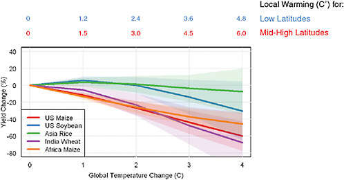
FIGURE O.5 Projected changes in yields of several crops worldwide as a function of global warming (relative to pre-industrial temperatures) in the absence of adaptation. Best estimates and likely uncertainty ranges are shown. {5.1}
demand for cereal crops can be expected to rise by about 25% over the same period. {5.1}
Up to roughly 2ºC global warming, studies suggest that crop yield gains and adaptation measures (especially in higher latitude areas) could balance yield losses in tropical and other regions, but warming above 2ºC is likely to increase global food prices. Major increases in trade of food from temperate to tropical areas are expected as a result of warming and represent one form of adaptation. Temperate growers are also likely to shift to earlier planting and longer maturing varieties as climate warms. However, adaptations are expected to be less effective in tropical regions where soil moisture, rather than cold temperatures, limits the length of the growing season. Very few studies have considered the evidence for ongoing adaptations to existing climate trends and have quantified the benefits of these adaptations. Future development of new varieties that perform well in hot and dry conditions may also promote adaptation, but the extent to which this will be effective remains unclear. At the higher warming scenarios considered in this report, it will be increasingly difficult to generate varieties with a physiology that can withstand extreme heat and drought while still being economically productive. Without adaptation, studies suggest that food prices could more than double if global warming were to be 5ºC. These estimates do not include additional losses due to weeds, insects, and pathogens, changes in water resources available for irrigation, effects of increased flood or drought frequencies, or responses to temperature extremes. {5.1}
Global warming of 2ºC would be expected to lead to average yield losses of U.S. corn of roughly 25% (±16% very likely range) unless effective adaptation measures are discovered and implemented. Nearly 40% of global corn production occurs in the United States, much of which is exported to other nations. The future yield of U.S. corn is therefore important for nearly all aspects of domestic and international agriculture. Higher temperatures speed development of corn and increase soil evaporation rates; further warming above 35ºC can compromise pollen viability, all of which reduce final yields. A major challenge in developing drought- and heat-tolerant varieties is that traits that confer these attributes often reduce yields in good years. {5.1}
Fire
Wildfire frequency and extent is expected to change in many countries as the global average temperature increases. Site-specific studies suggest that large increases in the area burned are expected in parts of Australia,
western Canada, Eurasia, and the United States. The primary driver of these changes is the warming in most of the regions evaluated, with lesser contributions from changes in precipitation. {5.4}
Areas of the United States that are particularly vulnerable to increases in wildfire extent include the Pacific Northwest and forested regions of the Rockies and the Sierra. Studies are limited in number but suggest that warming of 1ºC (relative to 1950-2003) is expected to produce increases in median area burned by about 200-400% (see Figure O.6). Some dry grassland and shrub regions (for example, in the southwestern United States) may experience a decrease in wildfires, because warming without increases in precipitation would reduce biomass production and hence limit the availability of fuel. Uncertainties include understanding of local soil moisture changes with global warming. Over time, extensive warming and associated wildfires could exhaust the fuel for fire in some regions, as forests are completely burned. {5.4}
Ocean Acidification
Rising atmospheric CO2alters ocean chemistry, leading to more acidic conditions (lower pH) and lower chemical saturation states for calcium carbonate minerals used by many plants, animals, and microorganisms to make shells and skeletons. Ocean acidification is documented clearly from ocean time-series measurements for the past two decades. Surface ocean pH has dropped on average by about 0.1 pH units from pre-industrial levels (pH is measured on a logarithmic scale, and a 0.1 pH drop is equivalent to a 26% increase in hydrogen ion concentration). Additional declines of 0.15 and 0.30 pH units will occur if atmospheric carbon dioxide reaches about 560 ppm and 830 ppm, respectively (see Figure O.7). Polar surface waters will become under-saturated with respect to aragonite, a key calcium carbon mineral, for atmospheric CO2 levels of 400-450 ppm for the Arctic and 550-600 ppm for the Antarctic. In tropical surface waters, large reductions in calcium carbonate saturation state will occur, but waters will remain super-saturated for projected atmospheric CO2 during the 21st century. Subsurface waters will also be affected, but more slowly, governed by ocean circulation; the fastest rates will occur in the upper few hundred meters globally and in polar regions where cold surface waters sink into the interior ocean. {4.9}
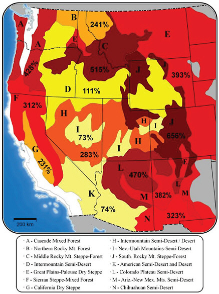
FIGURE O.6 Percent increase (relative to 1950-2003) in median annual area burned for ecoprovinces of the West with a 1ºC increase in global average temperature. Changes in temperature and precipitation were aggregated to the ecoprovince level using the suite of models in the CMIP3 archive. Climate-fire models were derived from National Clmatic Data Center (NCDC) climate division records and observed area burned data following methods discussed in Littell et al. (2009). {5.4}
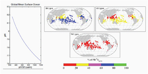
FIGURE O.7 (left panel) Variation in pH of global mean surface waters with CO2. (right panel) Global coral reef distribution and their net community calcification; the biological production of calcium carbonate skeleton or shell material, relative to their pre-industrial rate (280 ppm), in percent, taking into account both ocean acidification and thermal bleaching; the loss of algal symbionts in response to warming and other stressors, for each reef location at CO2 stabilization levels of 380, 450, and 560 ppm. Source: Silverman et al. (2009). {4.9; 5.8}
Impacts of CO2, pH, and Climate Change on Ocean Biology
The patterns and rates of ocean primary production will change due to higher sea surface temperatures and increased vertical stratification, altering the base of the marine food-web. Observations indicate a strong negative relationship between marine primary productivity and warming in the tropics and subtropics, most likely due to reduced nutrient supply, and low-latitude primary production is projected to decline on basin-scales under future climate warming. Primary production in some temperate and polar regions is projected to increase due to warming, reduced vertical mixing, and reduced sea ice cover. Subsurface oxygen levels are projected to decline due to warmer waters and altered ocean circulation, leading to an enlargement of oxygen minimum zones. {5.8}
The geographic range of many marine species is shifting poleward and to deeper waters due to ocean warming. Individual marine species will change differentially, for example with the ranges of pelagic fish likely changed more than those of demersal fish. Few studies have looked com-
prehensively across many marine taxa and geographic regions, but a recent study suggests the potential for significant changes in community structure in the Arctic and Southern Ocean biodiversity due to invasion of warm water species and high local extinction rates in the tropics and subpolar domains. {5.8}
Coral bleaching events will likely increase in frequency and severity under a warmer climate. Over the past several decades, warmer sea surface temperatures have led to widespread tropical coral bleaching events and increased coral mortality, and warming and more local human impacts are associated with declines in the health of coral reef ecosystems worldwide. Bleaching can occur for sea surface temperature changes as small as +1-2ºC above climatological maximal summer sea surface temperatures, which corresponds to global average warming of about 1.5-3ºC (Figures S.5 and O.7). {5.8}
Rising CO2and ocean acidification will likely reduce shell and skeleton growth by marine calcifying species such as corals and mollusks. Some studies suggest a threshold of 500-550 ppm CO2 whereby coral reefs would begin to erode rather than grow, negatively impacting the diverse reef-dependent taxa (see Figure O.7). Polar ecosystems also may be particularly susceptible when surface waters become undersaturated for aragonite, the mineral form used by many mollusks. Indirect impacts of ocean acidification on non-calcifying organisms and marine ecosystems as a whole are possible but more difficult to characterize from present understanding. {5.8}
Impacts of 21st Century Sea Level Rise
Depending on socioeconomic development, population growth, and intensity of adaptation, it has been projected that 0.5 m of sea level rise would increase the number of people at risk from coastal flooding each year by between 5 and 200 million; as many as 4 million of these people could be permanently displaced as a result. More than 300 million people currently live in coastal mega-deltas and mega-cities located in coastal zones. The corresponding projections for 1.0 m of sea level rise suggest that the number of people at risk of flooding each year would increase by 10 to 300 million. {5.2}
Coastal erosion is expected to occur as sea level rises with warming temperatures. Global aggregate estimates suggest that wetland and dry-land worldwide losses would sum to more than 250,000 km2 with 0.5 m of sea level rise; more than 90% of these losses are projected to occur in developing countries. {5.2}
Rising sea levels will impact key coastal marine ecosystems, coral reefs, mangroves, and salt marshes, through inundation and enhanced coastal erosion rates. Regional impacts will be influenced by local vertical land movements and will be exacerbated where the inland migration of ecosystems is limited by coastal development and infrastructure. {5.2}
Infrastructure Impacts
Climate change impacts on infrastructure—including transportation, buildings, and energy—are primarily driven by changes in the frequency and intensity of temperature extremes and heat waves, heavy rainfall and snow events, and sea level rise. Many impacts are directly tied to changes in climate thresholds, such as number of days above or below a certain temperature, or amount of rainfall accumulated in a 24-hour period, rather than mean temperatures. Extreme events confront infrastructure with conditions outside the range for which they were built; to the extent that these extreme events increase in a given region, vulnerability of infrastructure will increase. Studies clearly document substantial economic damages from past extreme events, but it is currently difficult to generalize any relationships between temperature change and the magnitude and/or cost of impacts across regions and sectors. {5.5}
Local conditions can magnify the susceptibility of infrastructure to climate-related impacts. High-risk locations include the Arctic and low-lying coastlines. Climate change impacts have already been observed in high-latitude and high-elevation areas built on permanently frozen ground. Impacts include increasing coastal erosion and shoreline damage from storms as sea ice retreats; and land-based impacts including a shorter land travel season and formation of cracks and sinkholes in the ground from melting permafrost. A significant amount of infrastructure is located in low-elevation regions at risk of flooding due to sea level rise and storm surge. Infrastructure in coastal areas includes cities, power stations, water treatment plants, roads and highways, homes and buildings, and oil and gas lines. {5.5}
Climate change is expected to increase electricity demand and affect production and reliability of supply. Observed correlations between daily mean near-surface air temperature and electricity demand suggest warmer summer temperatures, and more frequent, severe, and prolonged extreme heat events could increase demand for cooling energy. Increases in peak demand could be most severe in already heavily air-conditioned regions. At the same time, high temperatures combined with drought can threaten the
reliability of present-day electricity supply from hydropower and traditional generation sources, such as coal, gas, and nuclear, that require cooling water. {5.5}
Human Health
Heat-related illness and deaths occur as a direct result of sustained, elevated levels of extreme temperatures during heat waves, which are projected to increase with increasing temperatures. The frequency and severity of heat waves in Europe and North America are projected to increase under climate change. Under a 2ºC increase in global mean temperature, for example, the average number of days per year with maximum temperatures exceeding 38ºC or 100ºF across much of the south and central United States could increase by a factor of 3 relative to the 1961-1990 average. Under a 3.5ºC increase, the number of days is projected to increase by 5 to nearly 10 times. Some adaptation is inevitable as populations become accustomed to permanently different conditions. However, most research indicates that the public health impacts of climate change are likely to increase with temperature extremes; and new research highlights the potential that heat stress may impose hard limits on the inhabitability of some land areas under global temperature changes on the order of 10ºC or more. {5.5}
Climate change is likely to affect the geographic spread and transmission efficiency of illnesses and disease carried by hosts and vectors, but complexity precludes any quantitative estimates of the relationship between incidence of a given disease and temperature change. Confounding factors—involving viral, bacterial, plant, and animal physiology, as well as sensitivity to changes in climate extremes, including precipitation intensity and temperature variability—challenge attempts to resolve the influence of temperature on observed trends in disease incidence. Most recent projections suggest that the ranges of malaria and other diseases may shift, but increases in some areas will likely be accompanied by decreases in others. {5.5}
Climate change may exacerbate existing stressors, such as air pollution, water contamination, and pollen production. Warmer temperatures increase production of ground-level ozone, which affects respiratory health. For a given level of ozone precursor emissions, background ozone levels and days with high ozone pollution levels above a defined safety standard (or “ozone exceedances”) are projected to increase across much of the United States. Where heavy precipitation increases, risk of water contamination could also increase. Shifts in growing season, mean temperatures, and atmospheric
CO2 levels affect the length of the pollen season and the characteristics of the plans themselves, with some species shown to increase their pollen-producing capacity and even their toxicity. {5.6}
Ecology and Ecosystems
For at least the past 40 years, many species have been and are currently shifting the phenology (timing) of spring events in concert with warming temperatures. Examining 542 species of plants and 19 of animals, a large phenology (e.g., timing of blooming, egg laying, migrating) study of 21 European countries for the last 30 years of the 20th century found a total of 78% of species were shifting their spring phenology earlier and only 3% were shifting later. When combining all species showing change along with those in the same areas not showing a measurable change, species on average were found to change ~2.5 days per decade. Throughout the Northern Hemisphere the similar change was reported to be 2.3 days per decade. The magnitude of the change occurring only in those species showing a change on average was ~4 to ~5 days a decade. {5.7}
As the climate has warmed many species have been and are continuing to track this warming by shifting their ranges into areas that before warming were less hospitable due to cooler temperatures. Terrestrial species are moving toward the poles and up in elevation, while marine species are generally moving down to deeper waters. The average shift over many types of terrestrial species around the globe was about 6 km per decade. {5.7}
Historically, extinctions of most species have been found to be due to various stresses, such as land-use change, invasive species, and hunting, but now the vulnerability of many species to extinction is enhanced with the added stress placed upon them by climate change. Those species more prone to becoming in danger of extinction include those that have a maximum dispersal distance shorter than the distance to the closest “cool refuge” and those that are not a good colonizer and hence fail to become established in these cooler locations. {5.7}


