
4
Emissions Estimated from Atmospheric and Oceanic Measurements
The direct way to measure emissions of greenhouse gases from a source is to collect and analyze exhaust gases as they are emitted. To estimate regional or national emissions from a remote location, one can take advantage of the incomplete mixing of the atmosphere. Because of incomplete mixing, geographical variations in greenhouse gas emissions and removals cause the abundance of a gas to be elevated downwind of a source and reduced downwind of a sink. Measurements of gas abundances around the globe can be used to estimate the locations and sizes of the gas’s sources and sinks through tracer-transport inversion or inverse modeling (Box 4.1). Inverse modeling combines atmospheric and oceanic measurements with a model for atmospheric transport and mixing and models of the natural sources and sinks. Inverse modeling also works for estimates of oceanic sources and sinks, using measurements of greenhouse gases dissolved in water. Atmospheric and oceanic methods can be combined in joint atmosphere-ocean inversions (e.g., Jacobson et al., 2007a,b).
Although, in principle, tracer-transport inversion could provide independent estimates of anthropogenic emissions from individual countries for time scales of several days to a year, uncertainties using state-of-the-art methods are too high for this purpose. Four interacting factors are responsible for the large uncertainty:
-
Small signals. The emissions of the greenhouse gases covered in this report are small compared to the large atmospheric background. This means that anthropogenic emissions will increase the mole fraction of the gas (Box 1.3) by only a small percentage as air moves across a country (e.g., nitrous oxide [N2O] could be increased by 1 part per billion [ppb] over a global background of 320 ppb).
-
Incomplete understanding of atmospheric transport. To attribute a local increase in the abundance of a greenhouse gas to emissions by an upwind country, it is necessary to have an accurate reconstruction of air flow and mixing. Errors in the atmospheric transport model will cause errors in the inferred location and magnitude of emissions.
-
Large natural sources and sinks. Carbon dioxide (CO2), methane (CH4), and N2O all have large and uncertain natural sources and sinks that obscure the signals from anthropogenic emissions. For CO2, the instantaneous flux into and out of the terrestrial biosphere varies with time of day and season and can be an order of magnitude larger than fossil-fuel emissions.
-
Inadequate observing network. Many surface stations are located too far from intense natural and anthropogenic sources to enable robust determination of global trends and seasonal cycles. Although ground stations and aircraft measurements have been deployed in Europe and North America to study CO2 fluxes from urban and industrial regions, forests, cultivated land, and other terrestrial ecosystems, coverage of the globe is uneven and most countries are not adequately sampled.
Fortunately, technological and methodological remedies for these problems could be implemented within a few years, improving the capability for indepen-
|
BOX 4.1 Tracer-Transport Inversion A forward model of the atmospheric and/or oceanic abundance of a trace gas is based on solution of the continuity equation:  (1) The tendency in local abundance of species X at time t (∂X/∂t), written on the left as a finite difference over the time interval Δ, is equal to the local emission rate E into the volume being sampled plus in situ chemical production P minus loss rates L minus the divergence of the transport flux With current chemistry-transport models, this continuity equation is solved on a three-dimensional grid of more than a million points, using a meteorology (including winds, convection, diffusive mixing, clouds, and precipitation) that varies hourly. Most analyses today employ the Bayesian synthesis method (Enting, 2002; Gurney et al., 2003) that includes a priori estimates of emissions (the best estimate of the emission patterns, including uncertainties, obtained from independent data and modeling). In regions where the atmospheric measurements clearly constrain the emissions, the resulting a posteriori emissions are independent of the a priori; but in regions where the available measurements are inadequate for constraining the emissions, the method just returns what was assumed, the a priori. Thus, Bayesian methods result in more stable estimates of emissions, but sometimes add no new information. |
dently verifying self-reported emissions by countries. This chapter reviews studies that used tracer-transport inversion methods to estimate CO2 emissions and to check self-reported emissions of other greenhouse gases. The chapter also identifies four ways to reduce uncertainties associated with atmospheric monitoring of national CO2 emissions.
INVERSE MODELING STUDIES OF GREENHOUSE GAS EMISSIONS
Tracer-transport inversion methods have been used to estimate emissions of CO2, CH4, N2O, and hydrofluorocarbons (HFCs). This section summarizes the results of inverse modeling studies for estimating greenhouse gas emissions (especially CO2) and for checking self-reported emissions (especially chlorofluorocarbons [CFCs] and HFCs) at national to global scales.
Inversions of CH4, N2O, and HFCs
Top-down, atmospheric inverse model derivations of greenhouse gas emissions have been applied extensively to CO2, CH4, N2O, and the fluorinated gases. In general, these approaches use the patterns of variability in the trace gases to infer the geographic pattern of emissions, but they require some prior knowledge of the spatial and temporal patterns. For N2O, the Bouwman et al. (1995) work on uncertainties in the global distribution of emissions forms the core a priori data that are tested with atmospheric observations and models (Hirsch et al., 2006; Huang et al., 2008). Thus far, these studies, as well as similar ones for HFCs (e.g., Stohl et al., 2009), have been successful at testing the assumed emissions only at the scale of broad latitudinal bands. Some studies suggest that current observations and modeling are capable of providing information on individual country emissions (e.g., Manning et al., 2003), but these claims remain untested. Many such studies assume that the atmospheric transport model represents tracer transport perfectly and do not consider the large, uncharacterized errors in the models (e.g., Patra et al., 2003; Rayner, 2004; Prather et al., 2008).
A number of studies have derived top-down emission patterns for CH4 (e.g., Fung et al., 1991; Hein et al., 1997; Houweling et al., 1999), sometimes taking advantage of additional information contained in the relative isotopic abundances (e.g., 13CH4 versus 12CH4; Fletcher et al., 2004). These studies were able, for example, to verify the European Commission’s Emission Database for Global Atmospheric Research (EDGAR) inventory of CH4 emissions on a scale of North America to within an uncertainty of 20 percent, but they rely strongly on assumed patterns of emissions within the continent. Assimilation of satellite observations of CH4 (Bergamaschi et al., 2007; Meirink et al., 2008) may be able to constrain large emissions at a subnational level (e.g., rice paddies in India and Southeast Asia), but this has not yet been verified using a multimodel approach with realistic errors on the satellite data or by comparing predictions with regional inventories and surface observations. On the other hand, intense scientific campaigns involving regional measurements
and modeling (Kort et al., 2008; Zhao et al., 2009) have succeeded in deriving CH4 and N2O emissions at the subnational scale within the United States, although these short, intense campaigns cannot be sustained year-round over much of the globe.
One approach to quantifying regional emissions is to use the relative increase in abundances of several gases during pollution episodes to derive their relative emissions. For example, high-resolution time series of gases have been used to identify European pollution episodes and to quantify the relative emissions of halocarbons and N2O from Western Europe (Prather, 1985), as well as European emissions of dichloromethane, trichloroethene, and tetrachloroethene (Simmonds et al., 2006). This method has also been used to try to separate sources of CO2 by assuming that sulfur hexafluoride (SF6) is co-emitted with fossil-fuel combustion (Rivier et al., 2006; Turnbull et al., 2006). The approach obviates the need for accurate tracer-transport modeling and can define the relative emissions in a polluted air sample to 10 percent or better. However, it is limited to areas where distinct, single-source pollution plumes occur on top of a nearly uniform, clean air background. Surface-based, diurnal column measurements have recently been used to estimate CH4 emissions from the Los Angeles basin (Wunch et al., 2009). Two key criteria need to be met to derive absolute emissions, for example, of fossil-fuel CO2: (1) the absolute emissions of the reference gas must be known to equivalent or better accuracy; and (2) the two gases must be co-emitted in the same ratio over the entire region being sampled, otherwise the much larger errors in tracer-transport inversion dominate. Both criteria fail for SF6, but for 14CO2, the second criterion allows for the separation of fossil-fuel CO2 from biogenic sources (see “14C Measurements” below).
Overall, there are published cases for CH4, N2O, and the synthetic fluorinated gases in which one can distinguish source from sink and other cases in which one cannot. Thus, the committee estimates uncertainties in national emissions of these gases as 50 percent to greater than 100 percent.
CO2Emission Estimates
The long-term, accurate measurements of atmospheric CO2 at Mauna Loa by Keeling (1961) and many others (Figure 1.4) laid the foundation for much of our understanding of the carbon cycle, including the link between fossil-fuel combustion and increases in CO2 (Revelle and Suess, 1957; Pales and Keeling, 1965). Measurements of atmospheric CO2 and other gases are currently made at in situ stations (e.g., surface sites, towers, aircraft profiling) around the world (e.g., Figure 4.1, Appendix C) and from satellites. The combined use of CO2 and oxygen (O2) atmospheric measurements allows the CO2 removed from the atmosphere to be partitioned into land and oceanic carbon sinks (Keeling et al., 1993; Manning and Keeling, 2006; Denman et al., 2007). Observation of isotope analogues of CO2 (including 13C, 14C, 18O), CH4 (13C, 14C, D), and N2O (15N, 18O) as well as O2/N2 ratios have increased our understanding of the global sources and sinks of these greenhouse gases on scales of hemispheres or broad latitude bands. All of these measurements would significantly aid in verification or falsification of reported national emissions if the pattern of emissions being tested is provided and the measurements are made at sufficiently high spatial resolution and at suitable locations (e.g., within or close to the borders of the country whose emissions are being tested).
The mixing time of tracers in the atmosphere ranges from minutes to days between the ground and the tropopause, about two weeks around a latitude circle at midlatitudes, several months to reach through a hemisphere, about one year between the northern and southern hemispheres, and several years to mix through the stratosphere. The density of the observing network, together with the atmospheric mixing times, determines the spatial resolution with which sources and sinks can be inferred using an atmospheric model. In particular, the slow mixing between hemispheres and the preponderance of emissions in the northern hemisphere mean that the signal from anthropogenic emissions is relatively large when hemispheres are compared.
Tans et al. (1990) showed that the interhemispheric gradient in CO2 was smaller than it should have been, given the north-south disparity in fossil-fuel emissions. This implied a “missing sink” of more than one billion tons of carbon per year in the northern hemisphere. Subsequent analyses confirmed this qualitative conclusion but have struggled to improve its spatial resolution. Continued effort has focused on the range of different atmospheric model results and what model error could
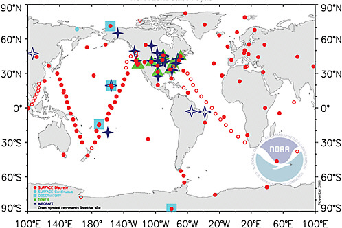
FIGURE 4.1 Map of the National Oceanic and Atmospheric Administration Earth System Research Laboratory (NOAA ESRL) global cooperative air sampling network in 2008. Blue squares are continuous measurements; red circles are weekly or daily flask samples; green triangles are continuous measurements on tall communications towers; and dark blue stars are weekly to biweekly vertical profiles by small aircraft. These sites provide a large fraction of the current set of atmospheric measurements of CO2 and related trace gases that are used in inverse modeling. SOURCE: NOAA ESRL, <http://www.esrl.noaa.gov/gmd/ccgg>.
do to CO2 inverse modeling (Engelen et al., 2002; Peylin et al., 2002; Gurney et al., 2003; Rayner, 2004; Baker et al., 2006a; Prather et al., 2008). The spread in north-south transport among the different models, while nonnegligible, is not large enough to invalidate interpretations of annual mean CO2 emissions from broad latitude bands. However, the derived emissions for each continent and ocean basin within each band are highly uncertain, even in sign. The addition or loss of a single site from the observing network in Figure 4.1, for example, can in some cases shift derived emissions for large regions, such as a half-continent, from positive to negative (e.g., Rödenbeck et al., 2003; Le Quéré et al., 2007; Law et al., 2003, 2008).
Transport uncertainty causes smaller systematic errors in changes in emissions than in their absolute magnitude. For example, Denman et al. (2007) compared emissions estimates from different tracer-transport models and found that year-to-year differences in estimates for different regions within the same latitude zone were surprisingly consistent between models, despite the large between-model differences in absolute magnitude. The implication is that it is easier to quantify changes in emissions than it is to assign absolute magnitudes to those emissions.
The first row of Table 4.1 summarizes the current state of the art in CO2 inversion estimates. It shows that although the annual atmospheric increase in CO2 is known within 7 percent, global annual fossil-fuel emissions can be estimated from atmospheric and
TABLE 4.1 Reducing Uncertainties in CO2 Emissions Through New Atmospheric and Ocean Observations
|
|
Decadal Global |
Annual Global |
Annual Regional |
Annual Continental |
Annual National |
||||||
|
Method |
Net Flux to the Atmosphere |
Net Flux to the Atmosphere |
Fossil Fuel |
IPCC LUCF |
Land-ocean Sink Partition |
Tropical Biosphere Changes |
Mid-latitude Biosphere Changes |
Fossil Fuel |
IPCC LUCF |
Fossil Fuel |
IPCC LUCF |
|
Current uncertainties |
|
|
|
|
|
|
|
|
|
|
|
|
State of art, including 13CO2, O2, oceanic, and atmospheric data |
1a (1%) |
1a (7%) |
2b (25%) |
5b |
5 |
5 |
5 |
5 |
|||
|
Potential improvements |
|
|
|
|
|
|
|
|
|
|
|
|
State of art plus 14CO2 |
|
|
1-2 |
5b |
2g |
2g |
2g |
2g |
5 |
2-4 |
5 |
|
All of the above plus intensive aircraft observations |
|
|
|
|
|
|
|
++g |
|
++g |
|
|
All of the above plus intensive ocean observations |
|
|
|
|
++g |
(+)g |
(+)g |
(+)g |
|
|
|
|
All of the above plus other tracers of combustion (e.g., CO, NOx, HCN) |
|
|
|
|
|
|
|
++ |
|
++ |
|
|
All of the above plus satellite CO2 observationsh |
|
|
|
|
++ |
++ |
++ |
++ |
|
++ |
|
|
NOTES: IPCC = Intergovernmental Panel on Climate Change; LUCF = land-use change and forestry. Other than %, units are Pg of CO2 per year for the 2000 decade. 1 = <10% uncertainty; 2 = 10-25%; 3 = 25-50%; 4 = 50-100%; 5 = >100% (i.e., cannot be certain if it is a source or sink). Potential improvements: ++ = likely and direct; (+) = indirect in the sense that it would directly improve estimates of ocean fluxes which, in a tracer-transport inversion, would reduce errors for land masses, especially for those at similar latitude. a2σ uncertainty of annual increase, P. Tans, <www.esrl.noaa.gov/gmd/ccgg/trends/>. bDenman et al. (2007). cConway et al. (1994); Ciais et al. (1995). dPeters et al. (2007). eGruber et al. (2009). fTans et al. (1990); Gurney et al. (2002). gImprove transport in models—expert judgment of committee. hIf systematic errors of satellite CO2 retrievals can be mastered through ongoing comparisons with in situ chemical measurements, frequent resampling can lead to the small errors of annual averages that are required for flux estimates. |
|||||||||||
oceanic data only to within 25 percent. The reason for the difference is the large interannual variation in the size of sources and sinks in the terrestrial biosphere and oceans, which must be separated from the total atmospheric increase to estimate the contribution from fossil fuel. Uncertainty in the anthropogenic emissions from land-use change and forestry is greater than 100 percent because both anthropogenic and natural changes in the terrestrial biosphere have almost identical effects on atmospheric CO2, 13C, and O2. For this reason, the inventory and remote sensing methods described in the previous chapters are needed for the a priori data on emissions from land use and forestry.
Because of transport uncertainty and the lack of measurements over much of the globe, estimates of the total net flux of CO2 from broad bands of latitude on a seasonal time scale are uncertain by at best 25-49 percent, compared to only 7 percent for the globe (Table 4.1). The situation is far worse for estimates of continental or national emissions (>100 percent) because east-west air flow rapidly mixes emissions signals and makes inversions sensitive to model error. In addition, there remains the question of whether the amplitude of the greenhouse gas perturbations caused by national emissions is large enough to detect with in situ networks or satellites.
Appendix B presents a mass-balance analysis for the 20-largest CO2 emitting nations. Table B.1 shows that anthropogenic emissions increase the abundance of CO2 by, on average, a fraction of a part per million (ppm) in the whole column (ranging from 0.06 ppm for Australia to 0.76 ppm for the United States). These small signals are measurable, but their detection is confounded by the much larger and incompletely understood signals from terrestrial ecosystems. Figure 4.2 shows that, even at global scales, and when fluxes are averaged over an entire year, the apparent fraction of fossil-fuel CO2 that remains in the atmosphere varies from year to year by as much as a factor of 2. Most of this variation is caused by the response of the terrestrial biosphere and oceans to climate anomalies (Francey et al., 1995; Keeling et al., 1995; Bacastow, 1976) and to increased fire activity during El Niño events (van der Werf et al., 2004, 2008). The magnitude of annual perturbations (sources or sinks) can be as large as one-quarter of the magnitude of global fossil-fuel emissions (e.g., Battle et al., 2000). To monitor anthropogenic emissions with tracer-transport inversion, one must be
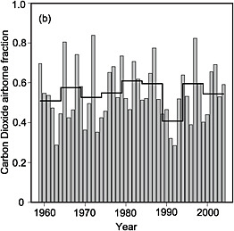
FIGURE 4.2 Interannual variation in the airborne fraction of fossil-fuel accumulation in the atmosphere. The airborne fraction is defined as the change in the mass of atmospheric CO2 divided by the mass of fossil-fuel CO2 emitted. The dark line shows successive 5-year averages. SOURCE: Figure 7.4b from IPCC (2007a), Cambridge University Press.
able to separate these terrestrial and ocean fluxes from the anthropogenic emissions.
Verification of CFCs, HFCs, and Other Synthetic Greenhouse Gas Emissions
The best tests of self-reported emissions using atmospheric chemistry models and observations have involved the global or hemispheric budgets of long-lived, synthetic, fluorinated gases produced solely by human activities. Rowland et al. (1982) measured CF2Cl2 at several remote sites to determine a global mean abundance. With knowledge of the long atmospheric lifetime (i.e., slow chemical loss), they were able to infer annual global emissions to high accuracy (e.g., 10 percent) from the annual increase in the atmosphere. The magnitude of CF2Cl2 emissions estimated from inverse modeling contradicted that claimed by the chemical industry, which subsequently retracted its reported emissions in favor of Rowland et al.’s derived emissions. This scenario was replayed in 2008 for the long-lived greenhouse gas NF3, which is used in rapidly increasing quantities in the manufacture of large flat-panel displays and photovoltaic cells. Prather and Hsu (2008) reviewed the production and lifetime of NF3, disputing an industry estimate of emissions (Robson et al., 2006) as unrealistically low and argued that this gas should be detectable and increasing in the atmosphere. Within months Weiss et al. (2008) made the measurements and confirmed that the reported NF3 emissions were indeed too low.
Inverse modeling based on atmospheric measurements also indicates much larger emissions of HFC-134a and SF6 than the sum of emissions in national inventories reported to the United Nations Framework Convention on Climate Change (UNFCCC). Höhne and Harnisch (2002) showed that post-1998 emissions of HFC-134a are 50 percent higher than reported by Annex I countries (see Figure 4.3), which are expected to be the source of nearly all HFC-134a emissions. Similar results have been shown for SF6 (Geller et al., 1997; Höhne and Harnisch, 2002). Although inverse modeling shows that emissions of many HFCs and CFCs are underestimated in UNFCCC inventories (and occasionally overestimated; see discussion of halon-1301 in Clerbaux and Cunnold, 2006), it offers no insight as to the source of error. Global or hemi-
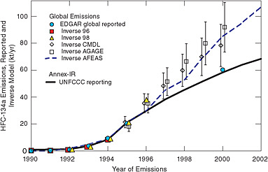
FIGURE 4.3 Global emissions of HFC-134a from several inverse atmospheric models, compared with UNFCCC reported Annex I emissions and the European Commission’s Emission Database for Global Atmospheric Research (EDGAR), for 1990-2002. Most production facilities and emissions for HFC-134a are in Annex I countries. SOURCE: Courtesy of Michael Prather, University of Cali-fornia, Irvine. Modified from Prather et al. (2009). Copyright 2009 American Geophysical Union. Reproduced by permission of the American Geophysical Union.
spheric inverse modeling can provide a strict test of the global sum of national greenhouse gas emissions inventories on an annual basis, but it has not been able to identify the countries whose emissions are in error.
NEW APPROACHES FOR INCREASING THE ACCURACY OF NATIONAL EMISSIONS ESTIMATES
Because of the twin problems of transport error and the separation of natural from anthropogenic fluxes, the uncertainty in tracer-transport inversion estimates of anthropogenic emissions for continents and nations can be as large as 100 percent (Table 4.1). These errors currently make tracer-transport inversion impractical for monitoring national emissions. Research is improving the representation of transport and biogeochemistry in models, but at the slow pace at which new observations are becoming available, advances cannot be expected to deliver the required accuracy during the coming decade. The following approaches, which would augment current research, would shift the observing paradigm for the carbon cycle and substantially improve our capability to monitor national emissions in the near term.
Measurements of Large Emission Sources
A large fraction of fossil-fuel emissions emanates from large local sources, such as cities or power plants, and thus the effect of national mitigation measures should be evident in the “domes” of CO2 that they produce (Idso et al., 2001; Pataki et al., 2003; Rigby et al., 2008a). For example, more than 57 percent of U.S. fossil-fuel emissions occur in areas that have a flux rate that exceeds 2 kg C m–2 yr–1, which corresponds to ~1.7 percent of the total surface area (including power plants, cities, and other point sources; Table 4.2). Cities also
TABLE 4.2 U.S. Fossil-Fuel Emissions as a Function of Carbon Density at 0.1 Degree Grid Spacing
|
Carbon Density of Emissions (kg C m–2yr–1) |
Area (%) |
Percentage of Total U.S. CO2Emissions |
|
≤2 |
98.3 |
42.7 |
|
2-4 |
0.9 |
13.6 |
|
4-10 |
0.6 |
18.0 |
|
10-20 |
0.2 |
15.1 |
|
20-max |
0.1 |
10.7 |
|
SOURCE: VULCAN emissions inventory; <www.purdue.edu/eas/carbon/vulcan>. |
||
provide a broad sample of different emission sectors (Table 4.3). Statistical or systematic sampling of CO2 emissions from large local sources would provide independent data against which to compare trends in emissions reported by the countries in which those sources are located, at least for fossil-fuel emissions. Sampling in cities, however, requires overcoming technical challenges, including finding ways to effectively construct seasonal averages in the presence of considerable spatial and daily variability and to separate biogenic from fossil-fuel sources (e.g., Pataki et al., 2003).
Working with large localized sources has two important advantages. First, their concentrated fossil-fuel emissions may be large enough to exceed the signal from local natural sources and sinks. For example, the emissions intensity of the greater Los Angeles metropolitan area (20 kg CO2 m–2 yr–1; see Table B.3) is ~20 times the annual net sink observed at Harvard Forest (0.9 kg CO2 m–2 yr–1; Barford et al., 2001), which is the difference between two much larger terms of opposite sign, photosynthesis and respiration. Of course, the sources and sinks in urban ecosystems are not as large as in Harvard Forest.
Second, large local sources increase the local CO2 abundance in the atmosphere by a few to more than 30 ppm, depending on proximity to local sources and atmospheric mixing (see Riley et al., 2008; Mays et al., 2009; and the analysis of signals from urban areas, power plants, and leaks from a geologic sequestration site in Appendix B). Because the increased CO2 abundances are largest over the source of emissions and disperse within a few tens of kilometers, they can usually be attributed unambiguously to their country of origin. This largely eliminates the attribution problem created by transport uncertainty in global tracer-transport inversions. For example, Figure 4.4 shows the size of the CO2 signature of a hypothetical large power plant in the Central Valley of California, as predicted by an atmospheric model. Although the CO2 plume at any given time varies with wind speed and direction, CO2 mole fractions would, on average, remain elevated above a continuously emitting power plant compared with the surroundings. In this way, the CO2 within a radius of the source could be used to infer emissions from power plants.
The CO2 domes created by large local sources can be mapped using measurements from surface stations and aircraft in and around cities, measurements of the radiocarbon content of annual plants found in urban environments, or measurements from high-resolution satellites.
Surface Network. The variability of CO2 and other greenhouse gases in cities is substantially greater than that measured at clean air marine boundary layer stations. Effective sampling of this variability in and
TABLE 4.3 CO2 Emissions for Selected Cities
|
|
|
|
Emissions |
||||
|
City |
Area (km2)a |
Population (millions) |
Total (Mton CO2yr–1) |
Commerce + industry (Mton CO2yr–1) |
Residential (Mton CO2yr–1) |
Utilities (Mton CO2yr–1) |
Transportation (Mton CO2yr–1) |
|
Los Angeles |
3,700 |
17.5 |
73.2 |
16.8 |
8.1 |
8.8 |
39.9 |
|
Chicago |
2,800 |
9.5 |
79.1 |
26.7 |
14.3 |
13.9 |
23.8 |
|
Houston |
3,300 |
5.5 |
101.8 |
48.8 |
2.2 |
32.6 |
20.1 |
|
Indianapolis |
900 |
2 |
20.1 |
3.7 |
2.2 |
5.5 |
8.8 |
|
Tokyo |
1,700 |
29b |
64 |
29.5 |
12.5 |
c |
22 |
|
Seoul |
600 |
13 |
43 |
18 |
13 |
12 |
|
|
Beijing |
800 |
15.6 |
74 |
57 |
12 |
5 |
|
|
Shanghai |
700 |
18b |
112 |
92 |
10 |
10 |
|
|
NOTE: Mton CO2 is million metric tons of CO2. aArea represents the contiguous area of intense activity, not administrative boundaries. Estimates of such functional boundaries were made from Google maps in “satellite” mode, which shows built up areas by color and road density. bTokyo does not include all of the agglomeration, which has 35 million inhabitants. The current population of Shanghai is 18.9 million, so emissions numbers are underestimates. cCO2 emissions are included in the commerce + industry and residential sectors. SOURCES: Dhakal et al. (2003) for population (including migrants) and emissions in 1998 for four east Asian cities. U.S. estimates are from the VULCAN emissions inventory for 2002 (<www.purdue.edu/eas/carbon/vulcan>) and the U.S. Census. |
|||||||
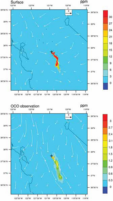
FIGURE 4.4 Instantaneous mole fraction of atmospheric CO2 at the surface (top) and averaged for the column using the Orbiting Carbon Observatory (OCO) averaging kernal (bottom) 24 hours after emissions from a hypothetical large power plant (emitting 4.16 million tons of carbon per year) at noon in the Central Valley of California. The simulation used the Weather Research and Forecast model (WRF), with meteorology for March 4, 2008, and the model resolution was 2 km. Note the difference in scales. Wind speed and direction for the surface and for the column are shown as white arrows. Since the hypothetical point source is located in the Central Valley, high CO2 at the surface is confined to the valley. Although there is vertical mixing, the emitted CO2 is confined to the lower 5 km of the atmosphere and thus would not be seen by AIRS (Atmospheric Infrared Sounder), which senses the upper troposphere. SOURCE: Courtesy of Zhonghua Yang and Inez Fung, University of California, Berkeley.
around cities is needed to estimate long-term mean values and to detect multiyear changes in emissions. Care must be taken in the sampling to integrate over the daily variations in emissions and meteorological conditions. A sampling network to measure the spatial gradients in greenhouse gases created by large local sources could be established for a sample of sites. The network would require ground-based stations and aircraft sampling. Airborne technologies to support such an effort are described in Appendix D. Enhanced automated meteorological observations in urban areas would help document the dispersion of CO2 and improve the estimation of local source strengths.
Urban Plants. Uptake of CO2 by plants integrates the 14C/12C ratio of CO2 in surface air over a period of several months during the growing season. The plants (by means of photosynthesis) provide long-term integrated samples during daytime periods when the planetary boundary layer is well developed and variability in CO2 is at a minimum. Decreases in the 14C/12C ratio of plant biomass are directly proportional to the level of excess fossil-fuel CO2 present, thus providing a seasonal measure of the dome of fossil-fuel CO2 over major metropolitan regions (Hsueh et al., 2007; Riley et al., 2008; Pataki et al., 2010). Figure 4.5 shows the distribution of atmospheric radiocarbon anomalies in the Los Angeles basin obtained from annual grasses.
By characterizing urban to suburban gradients, it may be possible to detect relative changes in fossil-fuel emissions over time. The 14CO2 measurements of annual plants using accelerator mass spectrometry are sufficiently accurate (2.7 permil; Riley et al., 2008) to detect a 6 percent change in fossil-fuel emissions. The actual detection limit will likely be higher because of year-to-year differences in the growing season of the sampled vegetation and variability in the synoptic-scale weather patterns. The preliminary observations shown in Figure 4.5 suggest that by sampling multiple locations repeatedly over several years, it would be feasible to detect an emissions change of ±15 percent within a large city. As with other approaches for urban air sampling, concurrent meteorological data and high-resolution tracer-transport modeling would be needed to reduce uncertainties associated with climatic variability of the atmospheric transport.
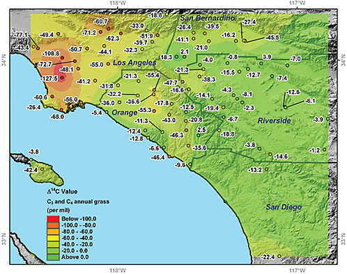
FIGURE 4.5 Radiocarbon anomalies (in permil) relative to background levels for Southern California. These anomalies were estimated relative to radiocarbon levels measured at Point Barrow, Alaska. One part per million of locally added fossil-fuel CO2 causes a radiocarbon decrease of –2.7 permil or –0.27 percent. The largest negative anomalies were observed near downtown Los Angeles and exceeded –100 permil, corresponding to over 35 ppm of locally added fossil-fuel CO2. Twenty sampling sites near downtown Los Angeles had a mean radiocarbon difference relative to Point Barrow, Alaska, of –58 permil, corresponding to a mean of 21 ppm of locally added fossil-fuel CO2. SOURCE: Courtesy of Wenwen Wang and James Randerson, University of California, Irvine. Modified from Figure 19.4 from Pataki et al. (2010). Reproduced with kind permission from Springer Science and Business Media.
The approaches described above for measuring large emission sources avoid some of the problems encountered in studies that have attempted to estimate natural or agricultural fluxes using atmospheric inversion techniques. First, it is possible to directly measure the fossil-fuel emissions that create a CO2 dome over a city or power plant. In contrast, accurate independent estimates of the actual integrated biological fluxes in a large region are not available. Second, whereas the concentration anomaly over a city or power plant has an unambiguous origin, transport errors make attribution uncertain for concentration anomalies over a natural or agricultural region.
A research program to measure the atmospheric dome of greenhouse gases over a representative sample of large local emitters would include three elements: (1) the development of new technologies and analysis approaches for detecting long-term trends in urban and industrial areas, (2) regional atmospheric modeling to help design the local network and to quantify variability from seasonally and interannually varying winds, and (3) comparison of different measurement techniques,
such as flask, isotope, aircraft, sun-viewing Fourier transform spectrometer, mobile platform, and satellite. Long-term monitoring could begin in approximately 10 different U.S. cities with different sizes, population densities, and different mixtures of emissions sources using currently available sampling technologies. Simultaneous creation of detailed bottom-up inventories of emissions for these same representative areas would facilitate transport modeling and enable the efficacy of different atmospheric approaches for trend detection to be assessed. By analogy with research initiatives of similar scope, this initiative would require a research budget of about $15 million to $20 million per year (e.g., $6 million to $10 million for extending National Oceanic and Atmospheric Administration [NOAA] flask and continuous monitoring to 10 cities and the remainder for technology development, modeling, and analysis) in the United States. Ideally, similar programs would be developed in other countries.
Satellites. By providing repeated global coverage from a single instrument, satellites would complement a global network of ground stations and aircraft sampling to monitor CO2 emitted from selected cities and power plants. They would also largely overcome the difficulties of national sovereignty and international cooperation in CO2 monitoring and the verification challenges associated with self-reporting. As shown in Table C.1 (Appendix C), Japan’s Greenhouse gases Observing Satellite (GOSAT) is the best available satellite for spaceborne measurement of CO2 anomalies from emissions. It has lower uncertainty and higher spatial resolution than the Scanning Imaging Absorption Spectrometer for Atmospheric Chartography (SCIAMACHY), the Atmospheric Infrared Sounder (AIRS), or the Infrared Atmospheric Sounding Interferometer (IASI), and it senses near the surface where emission signals are largest, unlike AIRS and IASI. However, the CO2 signal produced by the emissions of a large power plant is typically smaller than what can be measured with GOSAT. In contrast, the Orbiting Carbon Observatory (OCO), which failed on launch in February 2009, would have had the high spatial resolution required to monitor instantaneous CO2 emissions from such local sources.
For example, assume that a 500 MW pulverized coal power plant emits ~0.13 t s–1 of CO2 (e.g., 4 Mt CO2 yr–1) and that the wind speed is 3 m s–1. These conditions would produce a perturbation of approximately 0.5 percent (~1.7 ppm) in the average column abundance of CO2 within an OCO sample, which is consistent with the instrument’s design uncertainty of 1-2 ppm and significantly larger than the ground-tested value of 1 ppm. In contrast, because a GOSAT sample covers a larger area than an OCO sample, the CO2 perturbation within a GOSAT sample would be approximately 0.1 percent (~0.4 ppm). This is an order of magnitude smaller than GOSAT’s estimation error of 4 ppm. Note that in target mode, OCO could take up to 7,000 shots at an individual site, under different viewing angles, and could potentially have an uncertainty of 0.1 ppm if systematic biases were characterized and removed.
No other satellite has OCO’s critical combination of high precision, small footprint, readiness, density of cloud-free measurements, and ability to sense CO2 near the Earth’s surface (Table C.1, Appendix C). Its 1-2 ppm accuracy and 1.29 × 2.25 km sampling area would have been well matched to the size of a power plant. Yet, the OCO mission as planned would have had limitations for monitoring CO2 emissions from large sources because it would have sampled only 7-12 percent of the land surface (Miller et al., 2007) with a revisit period of 16 days and a nominal lifetime of only 2 years (Table C.1, Appendix C). However, many metropolitan areas are large enough to be sampled by the planned orbit, and OCO would still have provided a sample of a few percentage of the power plants.
Monitoring urban and power plant emissions from space is challenging and has not been demonstrated. A replacement OCO could demonstrate these capabilities. Nevertheless, it would be valuable to explore changes in the orbit and other parameters so that a greater fraction of large sources is sampled. For example, consider a precessing orbit covering ~100 percent of the surface but with only two measurements per year of each location. With 100-500 large local sources in high-emitting countries, it might be possible to obtain a statistical sample of hundreds of measurements of plumes of CO2 being emitted by the large sources in each of these countries. The trade-offs in optimizing monitoring capabilities while meeting scientific objectives (e.g., observing with high solar zenith angle) would have to be examined by a technical advisory group. The group
would also have to develop a strategy for integrating the snapshot view of CO2 anomalies from the satellite measurements into annual emissions.
Because of its 2-year mission life, OCO would not have been able to track emission trends. However, it would have provided the first few years of measurements (a baseline) necessary to verify a decadal trend for the large local sources within its footprint and served as a pathfinder for successor satellites designed specifically to support a climate treaty. Moreover, the technology used in the OCO instrument has no consumables or inherently short-lived components and hence could be flown on an extended, decadal mission. A replacement mission is expected to cost about the same as the original, $278 million.1 Alternate proposals to measure the near-surface CO2 abundance from space with multifrequency laser (e.g., the Active Sensing of CO2 Emissions over Nights, Days, and Seasons [ASCENDS] mission)2 are not yet technologically ready for long-term operations.
Deployment of a CO2-sensing satellite with the capability of OCO, together with a program of surface and aircraft sampling in and around large local sources would address all four main problems associated with tracer-transport inversion. It would enable the network to support emissions verification by observing CO2 directly over high-emitting sites, where the signal from anthropogenic emissions is locally large enough to separate from confounding natural fluxes and where the transport problem is far simpler than at regional and continental scales because emissions are in most cases still confined to the boundary layer. Ongoing sampling by aircraft or from balloons will be essential to investigate potential systematic biases of column abundances inferred from any satellite and to describe the vertical distribution necessary to infer the location of emissions.
A corresponding capability for other greenhouse gases does not exist, except for the ozone precursor NOx (nitrogen oxide). Satellite remote sensing of NOx emissions is readily able to detect decadal emission trends over urban and industrial regions (Martin et al., 2006; Stavrakou et al., 2008; Kaynak et al., 2009).
14C Measurements
Systematic radiocarbon (14C) measurements would largely eliminate the confounding effects of natural fluxes and thus greatly improve the accuracy of fossil-fuel emissions estimates. Carbon-14 is produced by cosmic rays in the higher layers of the atmosphere as well as from weapons tests. It is well mixed as 14CO2 in the lower atmosphere and oceans, where it is incorporated into all living organisms. Its radioactivity decays with a half-life of 5,730 years. Fossil fuels are formed from organic material, but their 14C component has fully decayed over millions of years. Thus, the CO2 emitted from the burning of fossil fuels is characterized by its absence of 14C, creating plumes of 14C-depleted air near source regions (Levin et al., 2003; Levin and Rödenbeck, 2008).
The addition of 1 ppm of fossil-fuel CO2 to a contemporary air mass with a background CO2 mole fraction of 390 ppm and a 14C/12C ratio typical of the free troposphere causes the 14C/12C ratio of CO2 to decrease by 0.27 percent (e.g., Turnbull et al., 2007). Accelerator mass spectrometry can measure 14C in CO2 in only 2 liters of ambient air to a precision of 0.2 percent. Comparison of the 14C depletion in an air sample to 14C measured in background air determines the CO2 component from recent fossil-fuel burning to a precision of 0.7 ppm, which is within the range of signals produced by fossil-fuel burning in individual nations (Table B.1, Appendix B).
Global 14CO2 observations would greatly reduce transport errors. The fossil-fuel emissions inventories of most Annex I countries are believed to be fairly accurate (Chapter 2). If a baseline of atmospheric 14CO2 observations can be established before emission reductions start taking hold, the observations would help constrain atmospheric mixing processes within transport models over the continents.
Box 4.2 presents an analysis of the kind of gains in estimation accuracy that could be realized from systematic 14C measurements if transport errors could be eliminated. The analysis shows that 10,000 14CO2 samples per year could yield fossil-fuel CO2 emission uncertainties of 10-25 percent in the United States. With a better designed sampling grid, only 5,000 samples may be needed to achieve that accuracy. In practice, 14CO2 measurements would likely provide
|
BOX 4.2 Gains from 14C Sampling A recent Observation System Simulation Experiment (OSSE) tested the capacity of 800 atmospheric 14CO2 measurements per month (e.g., Turnbull et al., 2007) to constrain U.S. fossil-fuel CO2 emissions. The results of the experiment are shown in the figure below. The left panel shows the total flux in 60 regions, as represented by the VULCAN emissions inventory. The right panel shows the uncertainty in the retrieval of the VULCAN emissions, which is treated as truth in this simulation. Note the change in color scale between the panels. Starting with an assumption of 100 percent uncertainty in the flux from each region, this simulation suggests that 14CO2 measurements can potentially determine the fossil-fuel flux in the coterminous United States to better than 10 percent. This OSSE was a test of the sampling density and assumed that the tracer-transport model was perfect. Errors in the tracer-transport model (as discussed here) would increase these uncertainties. 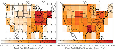 Estimation of CO2 fluxes from fossil-fuel burning using 10,000 14CO2 measurements per year. Left panel: Sources (VULCAN inventory; <www.purdue.edu/eas/carbon/vulcan>) aggregated into 5 × 5 degree areas (colored rectangles). The 84 virtual sampling locations, where virtual 14CO2 measurements were made every 3 days at 14:00 local time, are plotted as “pluses.” Right panel: Uncertainty of the total estimated flux in each 5 × 5 degree area. For both panels, January emissions and uncertainties are shown, but those for other months are not substantially different. SOURCE: Courtesy of John Miller, NOAA/ESRL. |
estimates of the global fossil-fuel flux that would be accurate enough to check trends from self-reported inventories collectively (Table 4.1). The accuracy of estimates of fossil-fuel CO2 emissions by continents would be expected to improve from >100 percent uncertainty to 10-25 percent uncertainty for intensely sampled regions, but national fossil-fuel CO2 emissions would still be uncertain at the 50-99 percent level if a country is not sampled intensely.
Making 14CO2 measurements in the air samples currently being collected in the global cooperative air sampling network (Figure 4.2) would be relatively inexpensive. It would cost only about $5 million to $10 million per year to collect and process the samples and to make the 14CO2 measurements on 10,000 samples per year. A dense deployment in the United States (5,000 samples per year) would provide proof of concept and identify its limits.
Measurement Programs to Reduce Model Errors
To improve estimates of national anthropogenic CO2 emissions from tracer-transport inversion, we will ultimately have to reduce transport errors in atmospheric models (see the plus signs in Table 4.1). Improvement of atmospheric tracer-transport models will require not only improved meteorological observations (especially of vertical mixing) but also new high-resolution measurements of multiple independent tracers that will enable the transport characteristics of the models to be validated. Such data are collected from international networks, supplemented by regional or global campaigns that measure multiple tracers with three-dimensional resolution, including vertical profiles. Previous and ongoing studies of this sort include the TRACE-P (TRAnsport and Chemical Evolution over the Pacific) campaign that examined the emis-
sions of CO from combustion in Asia (Kiley et al., 2003), the INTEX/NA (Intercontinental Chemical Transport Experiment—North America; Choi et al., 2008) that suggested stronger than expected vertical mixing, the regional campaign in the north central United States anchored by the WLEF tall tower in Wisconsin (Denning et al., 2003; Wang et al., 2007), and European efforts (e.g., see Ahmadov et al., 2007; Levin and Karstens, 2007; Vetter et al., 2008). To test and improve tracer-transport models, data on the time evolution of spatially resolved tracer abundances need to be accompanied by high-resolution gridded data on emissions (e.g., Gurney et al., 2009).
Although OCO would be capable of measuring large urban regions or power plants with precisions as great as 1-2 ppm (see Appendix C, Table C.1), much of the atmospheric signal from smaller or dispersed sources is much less than 1 ppm. Such signals can be measured accurately with in situ networks (e.g., surface sites, towers, aircraft profiling), such as the NOAA ESRL network (Figure 4.2) and the World Meteorological Organization (WMO) Global Atmosphere Watch (GAW) stations.3 However, many areas, including those with high greenhouse gas emissions, are not adequately sampled. For example, CO2 observations are sparse in the tropical latitudes, Africa, and South America. A number of recent studies have examined how to expand the current CO2 measurement sites to optimize the ability to retrieve CO2 emissions from transport modeling (Gloor et al., 2000; Patra et al., 2003; Rayner, 2004; Gurney et al., 2008). Expansion of the GAW network to observe the variations in greenhouse gas abundances in countries with the largest emissions would greatly improve the independent verification of emissions through tracer-transport modeling.
Expansion of the GAW network in the vertical dimension would allow more meaningful comparisons with satellite retrievals of column-averaged CO2 than ground-based measurements alone and would also provide a routine experimental check on how models transport emissions from the boundary layer to the free troposphere. With the cooperation of commercial airlines, calibrated high-precision measurements can be made routinely from regular flights at low cost. Although the transects are in the upper troposphere and lower stratosphere, a vertical profile is obtained during each takeoff and landing. Routine measurements of air pollutants have been made from European commercial airliners as part of the MOZAIC (since 1994) and CARIBIC (since 1997) research programs, and a successor program that will include CO2 and CH4 measurements (IAGOS) is being planned.4 Japanese scientists have obtained flask samples on JAL flights between Tokyo and Melbourne since 1993 and continuous measurements and flask samples onboard five aircraft traveling between Asia, Australia, Europe, and North America since 2005 (Machida et al., 2008).
Improvements to Tracer-Transport Inversion with Carbon Data Assimilation
The accuracy of sources and sinks inferred from variations of the atmospheric mole fraction is intimately tied to the accuracy of winds and mixing characteristics in tracer-transport models. Typically, wind and mixing data are obtained from a meteorological data assimilation system, wherein diverse streams of meteorological observations are merged with a numerical weather prediction (NWP) model to yield, every 3 or 6 hours, the best estimate of the atmospheric state and the uncertainty in the estimate. A reanalysis is undertaken occasionally to assimilate decades of meteorological observations into a single NWP model (e.g., Kalnay et al., 1996; Uppala et al., 2005) and, thus, represents the best source of information about climate variability on diurnal, seasonal, and interannual to decadal time scales. Most tracer-transport models or carbon data assimilation systems employ 3-hourly or 6-hourly atmospheric circulation statistics from a reanalysis.
Carbon data assimilation combines, in principle, emissions inventories and data on land use, greenhouse gas abundances, and meteorology with models of the atmosphere, ecosystems, and oceans into a coherent
|
3 |
See <http://www.wmo.int/pages/prog/arep/gaw/gaw_home_en.html>. |
|
4 |
See <http://www.iagos.org/> for a description of MOZAIC (Measurement of Ozone and Water Vapour on Airbus in-service Aircraft), CARIBIC (Civil Aircraft for the Regular Investigation of the Atmosphere Based on an Instrument Container), and IAGOS (In-service Aircraft for a Global Observing System). |
framework so that emission estimates can be constrained by their consistency with the other observations. Sources and sinks of CO2 and other greenhouse gases at the surface and in the atmosphere column can be derived, as has been demonstrated by the Observation System Simulation Experiment using CO2 from OCO (Baker et al., 2008), the two-step assimilation and inversion of AIRS CO2 (Chevallier et al., 2009; Engelen et al., 2009), and assimilation studies of satellite CO, CH4, and O3 using three-dimensional chemical transport models (Ménard et al., 2000; Clerbaux et al., 2001; Stajner et al., 2001; Meirink et al., 2008; Tangborn et al., 2009).
Most existing carbon data assimilation efforts are “univariate” in that they are carried out separately from the meteorological assimilation and neglect the spread in the reanalysis. As a result, consistency between the meteorology and trace gas mole fraction and fluxes is not guaranteed, and the quantifiable uncertainty in the circulation is not propagated into a spread in the trace gas mole fractions and, ultimately, to the sources and sinks. Examples of univariate assimilation projects include efforts to assimilate anticipated CO2 data from the OCO satellite into atmospheric models (Stajner et al., 2001; Baker et al., 2006b; Miller et al., 2007; Chevallier et al., 2007; Feng et al., 2009), the Oregon and California (ORCA) project, and NOAA’s CarbonTracker. The Observation System Simulation Experiments showed that the vast volume of OCO data (8,000,000 observations over 16 days) could yield improvements in CO2 source-sink estimates over continents with an error reduction of greater than a factor of 2 over land, although the degree of improvement depends on assumptions about errors and biases in the observations and models (Baker et al., 2008).
The ORCA project is a regional example of carbon data assimilation (Law et al., 2004; Quaife et al., 2008; Gökede et al., 2010). A terrestrial carbon flux model uses inputs of Landsat remote sensing data on disturbance history and land cover, and is calibrated with inventory biomass data and seasonal carbon and water fluxes from tower sites (Law et al., 2004). The improved model computes prior estimates of carbon fluxes for the land surface, including fluxes for land use and natural ecosystems. The output of the improved model is then used as input to an atmospheric transport model that links the estimated fluxes to atmospheric CO2 observations. This modeling component ingests three-dimensional meteorology, various remote sensing products (e.g., fraction of absorbed photosynthetically active radiation), fossil-fuel emission inventories, and time series of atmospheric CO2 mixing ratio data to produce regional estimates of surface fluxes that are used to evaluate regional representativeness of the prior estimated fluxes. Bayesian inversion is then applied to assign scaling factors that align the surface fluxes with the CO2 observation time series (Gökede et al., 2010). In this way, the model generates a record of its skill at predicting fluxes from natural ecosystems, agriculture, forestry, and land use, which should improve through time. The intent is to reduce uncertainties in fluxes over space and time, which should improve with increased density of atmospheric CO2 observations.
A quasi-operational global system is Carbon-Tracker, which inverts for net CO2 fluxes for land and ocean regions, with a high-resolution (1 × 1 degree latitude and longitude) zoom region over North America, using the boundary layer CO2 observing network (Peters et al., 2007). Net fluxes are adjusted each week by linear scaling factors for 209 land regions and 30 ocean regions. Emissions from fossil-fuel burning are held fixed. Initial estimates (before adjustment) are provided by the CASA-GFED2 model for terrestrial fluxes (van der Werf et al., 2006) and by an ocean inverse model for the ocean regions. Vertical profile data of CO2 from aircraft are used to validate the flux results and the modeled atmospheric transport. Uncertainties in the net CO2 emissions are estimated by comparing different configurations of the setup. Important limitations are (1) the sparseness of CO2 observations, which forces the assumption of coherent behavior of ecosystems over large distances; (2) the presumed pattern of fluxes, which dominate the high-resolution results; and (3) the accuracy of atmospheric transport and mixing in the model. In addition, some of the resulting emission patterns reflect primarily the a priori CASA-GFED2 model. However, on the scale of North America, CarbonTracker has consistently found net terrestrial uptake of 0.2 to 0.8 Pg C yr–1, varying year to year, which is not a feature of the CASA-GFED2 model.
The most sophisticated carbon data assimilation
to date is the Global and Regional Earth-System Monitoring Using Satellite and In-situ Data (GEMS) project (Hollingsworth et al., 2008),5 funded by the European Commission. The central atmospheric model is the European Centre for Medium-Range Weather Forecasts Integrated Forecast System (ECMWF IFS), which includes CO2 as a model prognostic variable, forced by prescribed surface sources and sinks. Radiance data from AIRS have been assimilated into the ECMWF IFS using the 4DVAR system to constrain the modeled atmospheric CO2 mole fraction in the upper troposphere. The assimilation consistently improves the meteorology, albeit slightly (McNally et al., 2006), and essentially creates, for the first time, gridded synoptic maps of CO2 in the midtroposphere (Engelen et al., 2009). The modeled upper-troposphere CO2 concentrations are then used as “observations” in a standard tracer-inversion step, thus updating the surface sources and sinks (Chevallier et al., 2009). These are promising new techniques, but the AIRS observations are weighted in the midtroposphere, so their ability to differentiate surface emissions from different countries is limited.
A new effort in the United States attempts to carry out a multivariate assimilation of meteorology and CO2 (Kang, 2009) using a carbon-climate model, so that uncertainties in the air flow and transport estimates are propagated to the trace gas variables, and the trace gas data inform the meteorological state, especially in regions with few wind observations. Early results suggest that the spread in the vertical profile of CO2 is on the order of 1 ppm due to the uncertainty in meteorological fields alone. With the simultaneous assimilation of AIRS CO2 observations, the spread in the CO2 profile grows to 1.5 ppm due to uncertainty in the AIRS observations and the propagation of spread in the meteorology to the CO2 forecast (Liu et al., 2009). This approach, if combined with accurate CO2 observations, especially near the surface, could effectively quantify the error due to imperfect knowledge of the meteorology, but leaves the errors due to numerical precision and coding structure of the tracer-transport model.
In addition to developing a fully coupled multivariate atmosphere-land-ocean carbon data assimilation system, it should be feasible to greatly improve several aspects of current data assimilation systems. A high spatial resolution nested subgrid could surround each observation site for a better representation of local meteorology. Multiple transport models and multiple source models of the oceans and terrestrial biosphere could be employed to “internalize” biases between different models as increased (and more realistic) uncertainty estimates. Expanded observation systems would increase the constraints, allowing less dependence on each site. Assumptions of coherent behavior of ecosystems over very large spatial scales could be relaxed because they are being made to compensate for the sparseness of observations.
RECOMMENDATIONS
The remote sensing programs described in Chapter 3 together with initiatives to measure 14CO2 and emissions from large local sources would significantly improve our capability to check self-reported emissions of CO2 (see Table 4.4). In particular, they would allow monitoring of land-use activities responsible for a large share of emissions from agriculture, forestry, and other land use and the significant portion of fossil-fuel emissions from countries that are produced by large local sources. They would also greatly improve our capacity to estimate total fossil-fuel emissions from continents. Implementation of initiatives to improve tracer-transport inversions would improve estimates for total fossil- and non-fossil-fuel emissions at the national level and for time scales ranging from daily to annual, enabling decadal changes to be detected. Specific recommendations include:
-
The National Aeronautics and Space Administration (NASA) should build and launch a replacement for the Orbiting Carbon Observatory. A technical advisory group should be convened to assess the optimal orbit and sampling strategies for estimating emissions from large local sources.
-
Extend the surface-based atmospheric sampling network to research the atmospheric “domes” of greenhouse gases over a representative sample (e.g., 5-10) of large local emitters, such as cities and power plants. Key goals of the research program would be (1)
|
5 |
See also GEMS, <http://gems.ecmwf.int>. GEMS concluded on May 31, 2009, and was replaced by a new project Modelling Atmospheric Composition and Climate (MACC). |
TABLE 4.4 Potential Improvements in National Emissions Estimates from Atmospheric and Oceanic Measurements and Models
-
to optimize trend detection using intensive sampling approaches, (2) to develop easily deployable and cost-effective sampling approaches for a globally extensive ground-based network, and (3) to provide a means for validating satellite measurements in these complex and understudied environments.
-
Extend the international WMO Global Atmospheric Watch network of in situ sampling stations to fill in underrepresented regions globally, thereby improving national sampling of regional greenhouse gas emissions. Expanding the network to increase collection of vertical profiles of greenhouse gases would constrain atmospheric transport and facilitate interpretation of satellite data. The vertical expansion could be done with the cooperation of commercial aircraft and with balloons flown to higher altitudes. Ideally, all major emitting nations and groups of neighboring smaller nations would participate in the cooperative network. The latter may require financial assistance and capacity building to aid the poorest nations that dominate the most undersampled regions.
-
Extend the capability of the existing CO2 sampling network to measure atmospheric 14C. At least one additional U.S. accelerator mass spectrometry laboratory is needed to handle approximately 10,000 new atmospheric 14CO2 samples a year.
-
An interagency group, with broad participation from the research community, should design a research program to develop gridded high-resolution data on U.S. fossil-fuel emissions and HFC, CFC, and PFC emissions. An important component of these maps should be uncertainty estimates that can be used directly in data assimilation programs. To support the research, the National Science Foundation (NSF), NOAA, NASA, and the Department of Energy should expand campaigns to sample the time evolution of tracer fields at high resolution as well as studies that use the data to improve transport modeling of tracers. This research would feed into an international initiative to publish gridded estimates for fossil-fuel emissions, as recommended in Chapter 2.
-
Develop a state-of-the-art carbon data assimilation system that is coupled and/or synergistic with meteorological, land, and oceanographic data assimilation systems for the United States. This would require new approaches for coupling circulation and biogeochemical models and for deriving biogeochemical properties (and hence surface fluxes) from the obser-
-
vations. It would also require enhanced collaboration among federal agencies with carbon observations, especially between NASA and NOAA, so that the best estimates and the uncertainties in the meteorology become integral components of emission estimation from a replacement OCO.
-
Sustain the infrastructure to measure natural sources and sinks on land and in the ocean, which must be separated from the total non-fossil-fuel flux to estimate agriculture, forestry, and other land-use (AFOLU) emissions. This requires sustaining the terrestrial flux network of sites (see Chapter 2)—augmented with high-precision, high-accuracy CO2 sampling for bottom-up and top-down model calibration—and continued measurements of the oceanic sink (see Appendix C).


