
Appendix C
Current Sources of Atmospheric and Oceanic Greenhouse Gas Data
ATMOSPHERIC DATA
The atmospheric monitoring sites of Mauna Loa and the South Pole, established during the 1957-1958 International Geophysical Year by C.D. Keeling, have been expanded to both remote and near continental sites (e.g., the ALE/GAGE [Atmospheric Lifetime Experiment-Global Atmospheric Gases Experiment] network, Prinn et al., 1983; the NOAA ESRL [National Oceanic and Atmospheric Administration Earth System Research Laboratory] network, Conway et al., 1994) and to include many other trace gases. The current global greenhouse gas measurement network is an international effort involving about 50 countries. It is coordinated by the World Meteorological Organization’s (WMO’s) Global Atmosphere Watch (GAW) Programme. The NOAA ESRL network, shown in Figure 4.2, is the largest contributing network to GAW. The WMO plays a crucial role in the international monitoring endeavor (1) by promulgating a common calibration scale for each species and quantitative goals for the comparability of measurements by participating laboratories; (2) by promoting comparison programs, measurement system audits, quality assurance and quality control guidelines, and submission of data to the World Data Center for Greenhouse Gases; and (3) by supporting capacity building.
Carbon dioxide (CO2) data are also available from three satellites—SCIAMACHY (Scanning Imaging Absorption Spectrometer for Atmospheric Chartography), AIRS (Atmospheric Infrared Sounder), and IASI (Infrared Atmospheric Sounding Interferometer)— and soon will be available from GOSAT (Greenhouse gases Observing Satellite), the first satellite designed for measuring CO2. A number of studies have used available satellite data to estimate atmospheric CO2 (e.g., Crevoisier et al., 2004, 2009; Buchwitz et al., 2005; Chahine et al., 2005, 2008; Maddy et al., 2008; Schneising et al., 2008; Strow and Hannon, 2008). Table C.1 contains information about the satellites as well as the Orbiting Carbon Observatory (OCO), which failed at launch on February 24, 2009. Unlike AIRS and IASA, OCO and GOSAT had a calibration system in place and a weighting function in the lower troposphere where the signal from surface emissions is strongest. OCO’s spatial resolution was more than an order of magnitude higher than any other satellite’s (instantaneous field of view <3 km2), and its signal-to-noise ratio was three times that of GOSAT.
OCEAN DATA
Carbon Dioxide
The accumulation of anthropogenic CO2 in the ocean resulting from atmospheric uptake can be readily observed. The inventory today is more than 500 billion tons and is increasing at a rate of >1 million tons per hour. Unlike the atmosphere and land surface, the oceanic CO2 signal is not amenable to satellite observation; seawater is a conducting medium and is impervious to electromagnetic radiation. Instead, CO2 is measured during large-scale observing expeditions at approximately decadal intervals. A few time-series stations are also maintained at locations where the changes
TABLE C.1 Specifications of Spaceborne Instruments Capable of Measuring CO2
|
Specification |
OCOa |
GOSATb |
SCIAMACHYc |
AIRSd |
IASIe |
|
Tropospheric gases measured |
CO2, O2 |
CO2, CH4, O2, O3, H2O |
O3, O4, N2O, NO2, CH4, CO, CO2, H2O, SO2, HCHO |
CO2, CH4, O3, CO, H2O, SO2 |
CO2, CH4, O3, CO, H2O, SO2, N2O |
|
CO2 sensitivity |
Total column including near surface |
Total column including near surface |
Total column including near surface |
Midtroposphere |
Midtroposphere |
|
Horizontal resolution (km)f |
1.29 × 2.25/5.2 |
FTS: 10.5/80-790 |
30 × 60/960 |
15/1,650 |
12/2,200 |
|
CO2 uncertainty (ppm)g |
1-2 |
4 |
14 |
1.5 |
2 |
|
Instruments |
3-channel grating spectrometer |
CAI, SWIR/TIR Fourier transform spectrometer |
8-channel grating spectrometer |
Grating spectrometer |
Fourier transform spectrometer |
|
Viewing modes |
Nadir, glint, target |
Nadir, glint, target |
Limb, nadir |
Nadir |
Nadir |
|
Samples per day |
500,000 |
18,700 |
8,600 |
2,916,000 |
1,296,000 |
|
Wavelength bandpass (μm) |
0.757-0.772, 1.59-1.62, 2.04-2.08 |
0.758-0.775, 1.56-1.72, 1.92-2.08, 5.56-14.3 |
0.24-0.44, 0.4-1.0, 1.0-1.7, 1.94-2.04, 2.265-2.38 |
3.74-4.61, 6.20-8.22, 8.80-15.4 |
3.62-5.0, 5.0-8.26, 8.26-15.5 |
|
Signal/noise (nadir, 5% albedo) |
>300 @ 1.59-1.62 μm, >240 @ 2.04-208 μm |
~120 @ 1.56-1.72 μm, ~120 @ 1.92-2.08 |
<100 @ 1.57 μm |
~2,000 @ 4.2 μm, ~1,400 @ 3.7-13.6 μm, ~800 @ 13.6-15.4 μm |
~1,000 @ 12 μm, ~500 @ 4.5 μm |
|
Orbit altitude |
705 km |
666 km |
790 km |
705 km |
820 km |
|
Local time |
13:30 ± 0:1.5 |
13:00 ± 0:15 |
10:00 |
13:30 |
21:30 |
|
Revisit time/orbits |
16 days/233 orbits |
3 days/72 orbits |
35 days |
16 days/233 orbits |
72 days/1,037 orbits |
|
Launch date |
Failed on launch |
January 2009 |
March 2002 |
May 2002 |
October 2006 |
|
Nominal life |
2 years |
5 years |
7+ years |
7+ years |
5 years |
|
NOTES: AIRS = Atmospheric Infrared Sounder; CAI = Cloud and Aerosol Imager; FTS = Fourier transform spectrometer; GOSAT = Greenhouse gases Observing Satellite; IASI = Infrared Atmospheric Sounding Interferometer; OCO = Orbiting Carbon Observatory; SCIAMACHY = Scanning Imaging Absorption Spectrometer for Atmospheric Chartography; SWIR = short-wavelength infrared; TIR = thermal infrared. aCrisp (2008); Crisp et al. (2008). bAkihiko Kuze, Japan Aerospace Exploration Agency, personal communication, 2009; Hamazaki et al. (2007); Shiomi et al. (2007). c<http://envisat.esa.int/instruments/sciamachy/>; Burrows et al. (1995); Noël et al. (1998); Buchwitz et al. (2005). dAumann et al. (2003); Chahine et al. (2008). ePhulpin et al. (2007); Crevoisier et al. (2009). fInstantaneous field-of-view/Swath. gThe uncertainty represents the estimate of random errors (e.g., the effects of detector noise) and additional systematic errors (e.g., bias caused by cloud and aerosol effects) unaccounted for or otherwise eliminated from the total error. Bias is reduced by successful validation efforts. The GOSAT uncertainty is dominated by the precision (random errors). For OCO, Crisp et al. (2004) and Miller et al. (2007) discuss the observational system simulation experiments, including modeling of the OCO instrument performance characteristics, that led to an instrument design that would meet a measurement requirement of 1 part per million (ppm). The as-built OCO instrument performance was verified during prelaunch tests, which included direct solar observations. The analysis of the latter gave the best confirmation that the as-built instrument performance exceeded its design requirements. The methods for bias reduction and validation are the same for GOSAT and OCO. Washenfelder et al. (2006) demonstrated the OCO validation concept and the essential role of ground-based measurements for meeting those objectives. Bösch et al. (2006) used these ground-based measurements to validate SCIAMACHY CO2. The GOSAT team also plans to use the same validation sites and instruments. OCO planned to include and use Aeronet measurements. The OCO validation plan purposely located ground-based validation measurements at Atmospheric Radiation Measurement (ARM) Program sites to capitalize on the wealth of ancillary atmospheric and surface measurements. |
|||||
can be directly measured on shorter time scales. Time trends in oceanic CO2 at a single point are illustrated in Figure C.1. Most well-qualified oceanic CO2 datasets reside at the Department of Energy’s Carbon Dioxide Information Analysis Center.1
Early work to track the accumulated burden of anthropogenic CO2 in seawater relied on tracer data, such as bomb 14C. The use of tracers was necessary because of the high natural background level of dissolved CO2 in seawater, the complexity of the processes affecting its distribution, and the relatively small size of the anthropogenic signal, all of which combined to make direct observation an uncertain business. Today, there are widely available accurate standards and mea-
|
1 |
See <http://cdiac.ornl.gov/>. |
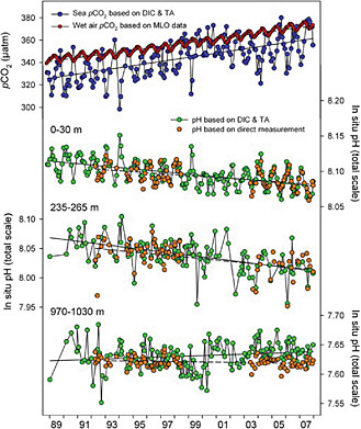
FIGURE C.1 Time trend of surface water pCO2 offshore Hawaii, showing the direct tracking with atmospheric CO2 forcing and the resultant change in ocean pH. The change in pH results from reaction with dissolved carbonate ion and causes a decline in the buffer capacity of seawater. The penetration to depth can also be seen in the changing subsurface data. SOURCE: Dore et al. (2009). Copyright 2009 National Academy of Sciences, U.S.A.
surements, greatly improved knowledge of the functioning of natural cycles, and an enormous increase in the anthropogenic CO2 signal.
The first demonstrated recovery of the anthropogenic CO2 signal from direct ocean measurements was by Brewer (1978), who corrected for the subsurface changes in dissolved CO2 due to respiration and carbonate dissolution and showed that the residual pCO2 signal closely resembles the atmospheric CO2 history of the water mass. An additional term to correct for local air-sea disequilibrium at the water mass source was applied by Gruber et al. (1996), and techniques such as these are widely used today. In addition, comparison of datasets from different cruise years now allows simple tracking of the changing ocean anthropogenic CO2 burden. An example of the ability to record the increasing storage of anthropogenic CO2 in the ocean is shown in Figure C.2.
Methane
The chemistry of ocean methane (CH4) is complex (see the review by Reeburgh, 2007); determining the extent to which the atmosphere is affected and detecting and understanding regional changes (e.g., ocean basin scale, or preferably less) are considerable challenges. First, the global methane budget contains significant oceanic terms (Table C.2). The net ocean emissions to the atmosphere are only about 2 percent of the total, mostly because large amounts of methane originating in
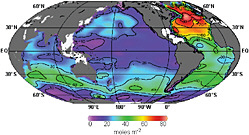
FIGURE C.2 Column inventory of anthropogenic CO2 in the ocean as of 1994. The accumulated burden is 388 ± 62 billion tons CO2 and is growing at a rate of ~7.4 billion tons per year. Thus, the inventory in 2009 is ~500 billion tons CO2. SOURCE: Figure 1 from Sabine et al. (2004). Reprinted with permission from AAAS.
continental margin sediments are consumed by microbial processes before they can be released into the fluid ocean. The terms for methane hydrate decomposition and release and for tracing the signature of gas plumes emitted from the seafloor, which can affect regional signals, are being updated rapidly.
Ocean Water Column. The first ocean water column measurements of methane were made in the late 1960s (Swinnerton and Linnenbom, 1967), revealing nanomolar concentrations and values well below atmospheric equilibrium at depth, indicating oceanic consumption within the water column. Measurements of oceanic profiles by Scranton and Brewer (1977) showed the puzzling existence of a significant maximum in concentration just below the oceanic mixed layer, a pattern later found over large regions of the global ocean (Watanabe et al., 1995). The puzzle was likely solved by Karl et al. (2008), who documented aerobic production of methane by decomposition of methyl phosphonate when consumed by phytoplankton in phosphate-starved environments. This process likely accounts for the small net source of CH4 to the atmosphere from the upper ocean (Table C.2). Thus, observations of a peak in methane concentrations in the upper ocean should not be confused with industrial releases.
TABLE C.2 Global Net Methane Emissions
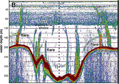
FIGURE C.3 Acoustic signatures of methane plumes rising from the floor of the Black Sea offshore from the Crimean peninsula. SOURCE: McGinnis et al. (2006). Copyright 2006 American Geophysical Union. Reproduced by permission of the American Geophysical Union.
Methane in the upper ocean, whether transferred there by exchange with the atmosphere or created locally, is consumed through oxidation to CO2 as the water masses are transferred to depth (Scranton and Brewer, 1978). The recent rise in atmospheric CH4 concentrations is imprinted on this process (Rehder et al., 1999); methane originating in the deep sea around vents is also quickly consumed.
Venting of Methane from the Seafloor. Methane is vented naturally from the large reservoirs on the continental shelves, but little reaches the atmosphere. For example, Figure C.3 shows the acoustic detection of a field of methane plumes rising from the floor of the Black Sea (Schmale et al., 2005; McGinnis et al., 2006). Although the height of the plumes (some are higher than 1,300 m) is impressive, little of the gas is vented to the atmosphere. The reason is that gas bubbles venting from the seafloor become coated with a film of hydrate (CH4.6H2O) or oily material from the higher hydrocarbons, which slows the dissolution rate of the rising bubble by about a factor of 4 (Rehder et al., 2002). The Black Sea is an unusual case because the deep water is anoxic and the density contrast between deep and surface layers is very strong. Nonetheless, both observations and models show that even the largest plumes undergo such significant dissolution during their rise to the surface that only plumes originating from very shallow sources (~100 m depth) can provide a source of oceanic CH4 to the atmosphere.
Satellites. The use of satellites to detect and quantify methane releases from the ocean has received little attention. The most novel and useful approach was taken by MacDonald and colleagues (MacDonald et al., 2008), who used synthetic aperture radar (SAR) imagery of the Gulf of Mexico to provide a basinwide inventory of gas seeps based upon their surface expression. The team identified some 1,821 sources and estimated the methane emissions to the atmosphere. The effect seen in the SAR imagery (Figure C.4) is the damping of capillary waves from the trace oil residue carried on the rising bubbles and reaching the sea surface. A pure methane gas stream with zero associated
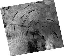
FIGURE C.4 SAR image of the Gulf of Mexico showing the surface expression of gas seeps from the trace oil components. SOURCE: MacDonald et al. (2008). Copyright 2008 American Geophysical Union. Reproduced by permission of the American Geophysical Union.
higher hydrocarbons would not show this effect, but the oil-gas association is very common.
Methane Hydrates. Releases of CH4 from methane hydrates are uncertain (see the question mark in Table C.2). Although vast quantities of hydrates are known to occur in nature, recent estimates range from 500-2,500 Gt C (Milkov, 2004) to 63,400 Gt C (Klauda and Sandler, 2005). A map of known hydrate locations is shown in Figure C.5.
The potential for global warming to destabilize seafloor methane hydrates has been debated since the early 1980s (e.g., Revelle, 1983). The quantities are so large that destabilization of hydrates could be of grave concern. Fortunately, the danger seems small; almost all of the methane released from seafloor hydrates would simply dissolve into the surrounding water and then be microbially oxidized to CO2 (Hester and Brewer, 2009).
Nitrous Oxide
The oceans are a source of N2O to the atmosphere, emitting some 25-33 percent of the total flux (Hirsch et al., 2006). However, using this information to assign fluxes to any specific region, or decoding the oceanic component of trends over reasonable periods of time (a decade or so), will be exceptionally difficult. The concentration of dissolved N2O in seawater is nanomolar.
The source of N2O in the ocean is intimately
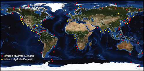
FIGURE C.5 Worldwide map of more than 90 hydrate occurrences; such sites could be monitored from space for evidence of methane releases. SOURCE: Hester and Brewer (2009). Reproduced with permission of Annual Reviews, Inc.; permission conveyed through Copyright Clearance Center, Inc.
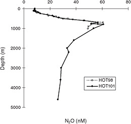
FIGURE C.6 Typical oceanic depth profile of dissolved N2O, observed at the Hawaii Ocean Time Series station. The presence of higher levels of N2O is strongly correlated with the oxygen minimum. SOURCE: Reprinted from Ostrom et al. (2000) with permission from Elsevier.
involved with microbial transformations of nitrogen compounds and shows strong spatial heterogeneity. The intense subsurface low-oxygen regions of the northern Indian Ocean have been shown to be a significant source (Law and Owens, 1990) of N2O production, but transfer of the gas to the atmosphere occurs erratically with wind-driven events. Stable isotope evidence suggests that the well-oxygenated upper water column in subtropical waters is a large source of atmospheric N2O (Dore et al., 1998), but the broad pattern is consistent with production of N2O in low-oxygen regions during the nitrification process (Nevison et al., 2003). A plot of a typical oceanic profile is shown in Figure C.6.
It is widely recognized that under a warming climate scenario, deep ocean oxygen levels will decline. Thus, models have used the relationship between N2O and O2 to predict strongly increased N2O fluxes from the future ocean (Schmittner et al., 2008; Shaffer et al., 2009). For example, Schmittner et al. (2008) estimate that by the year 4000, atmospheric N2O will increase by about 21 percent as a result of this increased oceanic flux as a weak positive feedback. However, these very long term effects are likely to have little impact on twenty-first century treaty monitoring.
REFERENCES
Aumann, H.H., M.T. Chahine, C. Gautier, M.D. Goldberg, E. Kalnay, L.M. McMillin, H. Revercomb, P.W. Rosenkranz, W.L. Smith, D.H. Staelin, L.L. Strow, and J. Susskind, 2003, AIRS/ AMSU/HSB on the Aqua Mission: Design, science objectives, data products, and processing systems, IEEE Transactions on Geoscience and Remote Sensing, 41, 253.
Bösch, H., G.C. Toon, B. Sen, R.A. Washenfelder, P.O. Wennberg, M. Buchwitz, R. deBeek, J.P. Burrows, D. Crisp, M. Christi, B.J. Connor, V. Natraj, and Y.L. Yung, 2006, Space-based near-infrared CO2 measurements: Testing the OCO retrieval algorithm and validation concept using SCIAMACHY observations over Park Falls, Wisconsin, Journal of Geophysical Research, 111, D23302, doi:10.1029/2006JD007080.
Brewer, P.G., 1978, Direct observation of the oceanic CO2 increase, Geophysical Research Letters, 5, 997-1000.
Buchwitz, M., R. de Beek, S. Noël, J.P. Burrows, H. Bovensmann, H. Bremer, P. Bergamaschi, S. Körner, and M. Heimann, 2005, Carbon monoxide, methane and carbon dioxide columns retrieved from SCIAMACHY by WFM-DOAS: Year 2003 initial data set, Atmospheric Chemistry and Physics, 5, 3313-3329.
Burrows, J.P., E. Hölzle, A.P.H. Goede, H. Visser, and W. Fricke, 1995, SCIAMACHY—Scanning Imaging Absorption Spectrometer for Atmospheric Chartography, Acta Astronautica, 35, 445-451.
Chahine, M., C. Barnet, E.T. Olsen, L. Chen, and E. Maddy, 2005, On the determination of atmospheric minor gases by the method of vanishing partial derivatives with application to CO2, Geophysical Research Letters, 32, L22803, doi:10.1029/ 2005GL024165.
Chahine, M.T., L. Chen, P. Dimotakis, X. Jiang, Q. Li, E.T. Olsen, T. Pagano, J. Randerson, and Y.L. Yung, 2008, Satellite remote sounding of mid-tropospheric CO2, Geophysical Research Letters, 35, L17807, doi:10.1029/2008GL035022.
Conway, T.J., P.P. Tans, L.S. Waterman, K.W. Thoning, D.R. Kitzis, K.A. Masarie, and N. Zhang, 1994, Evidence for interannual variability of the carbon cycle from the NOAA/GMCC global air sampling network, Journal of Geophysical Research, 99, 22,831-22,855.
Crevoisier, C., S. Heilliette, A. Chedin, S. Serrar, R. Armante, and N.A. Scott, 2004, Midtropospheric CO2 concentration retrieval from AIRS observations in the tropics, Geophysical Research Letters, 31, L17106, doi:10.1029/2004GL020141.
Crevoisier, C., A. Chedin, H. Matsueda, T. Machida, R. Armante, and N.A. Scott, 2009, First year of upper tropospheric integrated content of CO2 from IASI hyperspectral infrared observations, Discussion, Atmospheric Chemistry and Physics, 9, 8187-8222.
Crisp, D., 2008, The Orbiting Carbon Observatory: NASA’s first dedicated carbon dioxide mission, in Sensors, Systems, and Next-Generation Satellites XII, Proceedings of SPIE, 7106, 710604.
Crisp, D., R.M. Atlas, F.-M. Breon, L.R. Brown, J.P. Burrows, P. Ciais, B.J. Connor, S.C. Doney, I.Y. Fung, D.J. Jacob, C.E. Miller, D. O’Brien, S. Pawson, J.T. Randerson, P. Rayner, R.J. Salawitch, S.P. Sander, B. Sen, G.L. Stephens, P.P. Tans, G.C. Toon, P.O. Wennberg, S.C. Wofsy, Y.L. Yung, Z. Kuang, B. Chudasama, G. Sprague, B. Weiss, R. Pollock, D. Kenyon, and S. Schroll, 2004, The Orbiting Carbon Observatory (OCO) mission, Advances in Space Research, 34, 700-709.
Crisp, D., C.E. Miller, and P.L. DeCola, 2008, NASA Orbiting Carbon Observatory: Measuring the column averaged carbon dioxide mole fraction from space, Journal of Applied Remote Sensing, 2, 023508, doi:10.1117/1.2898457.
Dore, J.E., B.N. Popp, D.M. Karl, and F.J. Sansone, 1998, A large source of atmospheric nitrous oxide from subtropical North Pacific surface waters, Nature, 396, 63-65.
Dore, J.E., R. Lukas, D.W. Sadler, M.J. Church, and D.M. Karl, 2009, Physical and biogeochemical modulation of ocean acidification in the central North Pacific, Proceedings of the National Academy of Sciences, 106, 12,235-12,240.
Gruber, N., J.L. Sarmiento, and T.F. Stocker, 1996, An improved method for detecting anthropogenic CO2 in the oceans, Global Biogeochemical Cycles, 10, 809-837.
Hamazaki, T., Y. Kaneko, A. Kuze, and H. Suto, 2007, Greenhouse gases observation from space with TANSO-FTS on GOSAT, in Fourier Transform Spectroscopy/Hyperspectral Imaging and Sounding of the Environment, Optical Society of America Technical Digest Series, paper FWB1.
Hester, K.C., and P.G. Brewer, 2009, Clathrate hydrates in nature, Annual Review of Marine Science, 1, 303-327.
Hirsch, A.I., A.M. Michalak, L.M. Bruhwiler, W. Peters, E.J. Dlugokencky, and P.P. Tans, 2006, Inverse modeling estimates of the global nitrous oxide surface flux from 1998-2001, Global Biogeochemical Cycles, 20, GB1008, doi:10.1029/2004GB002443.
Karl, D.M., L. Beversdorf, K.M. Bjorkman, M.J. Church, A. Martinez, and E.F. DeLong, 2008, Aerobic production of methane in the sea, Nature Geoscience, 1, 473-478.
Klauda, J.B., and S.I. Sandler, 2005, Global distribution of methane hydrate in ocean sediment, Energy & Fuels, 19, 459-470.
Law, C.S., and N.J.P. Owens, 1990, Significant flux of atmospheric nitrous oxide from the northwest Indian Ocean, Nature, 346, 826-828.
MacDonald, I.R., V. Asper, O. Garcia, M. Kastner, I. Leifer, T.H. Naehr, E. Solomon, S. Yvon-Lewis, and B. Zimmer, 2008, HyFlux—Part 1: Regional modeling of methane flux from near-seafloor gas hydrate deposits on continental margins, American Geophysical Union, fall meeting, abstract OS33A-1322.
Maddy, E.S., C.D. Barnet, M. Goldberg, C. Sweeney, and X. Liu, 2008, CO2 retrievals from the Atmospheric Infrared Sounder: Methodology and validation, Journal of Geophysical Research, 113, D11301, doi:10.1029/2007JD009402.
McGinnis, D.F., J. Greinert, Y. Artemov, S.E. Beaubien, and A. Wüest, 2006, Fate of rising methane bubbles in stratified waters: How much methane reaches the atmosphere? Journal of Geophysical Research, 111, C09007, doi:10.1029/2005JC003183.
Milkov, A.V., 2004, Global estimates of hydrate-bound gas in marine sediments: How much is really out there? Earth-Science Reviews, 66, 193-197.
Miller, C.E., D. Crisp, P.L. DeCola, S.C. Olsen, J.T. Randerson, A.M. Michalak, A. Alkhaled, P. Rayner, D.J. Jacob, P. Suntharalingam, D.B.A. Jones, A.S. Denning, M.E. Nicholls, S.C. Doney, S. Pawson, H. Bösch, B.J. Connor, I.Y. Fung, D. O’Brien, R.J. Salawitch, S.P. Sander, B. Sen, P. Tans, G.C. Toon, P.O. Wennberg, S.C. Wofsy, Y.L. Yung, and R.M. Law, 2007, Precision requirements for space-based XCO2 data, Journal of Geophysical Research, 112, D10314, doi:10.1029/2006JD007659.
Nevison, C., J.H. Butler, and J.W. Elkins, 2003, Global distribution of N2O and the N2O-AOU yield in the subsurface ocean, Global Biogeochemical Cycles, 17, 1119, doi:10.1029/2003GB002068.
Noël, S., H. Bovensmann, J.P. Burrows, J. Frerick, K.V. Chance, A.P.H. Goede, and C. Muller, 1998, The SCIAMACHY instrument on ENVISAT-1, in Sensors, Systems, and Next-Generation Satellites II, Proceedings of SPIE, 3498, 94-104.
Ostrom, N.E., M.E. Russ, B. Popp, T.M. Rust, and D.M. Karl, 2000, Mechanisms of nitrous oxide production in the subtropical North Pacific based on determinations of the isotopic abundances of nitrous oxide and di-oxygen, Chemosphere—Global Change Science, 2, 281-290.
Phulpin, T., D. Blumstein, F. Prel, B. Tournier, P. Prunet, and P. Schlüssel, 2007, Applications of IASI on MetOp-A: First results and illustration of potential use for meteorology, climate monitoring, and atmospheric chemistry, in Atmospheric and Environmental Remote Sensing Data Processing and Utilization III: Readiness for GEOSS, Proceedings of SPIE, 6684, 66840F.
Prinn, R.G., P.G. Simmonds, R.A. Rasmussen, R.D. Rosen, F.A. Alyea, C.A. Cardelino, A.J. Crawford, D.M. Cunnold, P.J. Fraser, and J.E. Lovelock, 1983, The Atmospheric Lifetime Experiment 1, Introduction, instrumentation, and overview, Journal of Geophysical Research, 88, 8353-8367.
Reeburgh, W.S., 2003, Global methane biogeochemistry, in The Atmosphere, Treatise on Geochemistry, 4, R.F. Keeling, H.D. Holland, and K.K. Turekian, eds., Elsevier-Pergamon, Oxford, U.K., pp. 65-89.
Reeburgh, W.S., 2007, Oceanic methane biogeochemistry, Chemical Reviews, 107, 486-513.
Rehder, G., R. Keir, E. Suess, and M. Rhein, 1999, Methane in the Northern Atlantic controlled by microbial oxidation and atmospheric history, Geophysical Research Letters, 26, 587-590.
Rehder, G., P.G. Brewer, E.T. Peltzer, and G. Friederich, 2002, Enhanced lifetime of methane bubble streams within the deep ocean, Geophysical Research Letters, 29, 10.1029/2001GL013966.
Revelle, R.R., 1983, Methane hydrates in continental slope sediments and increasing carbon dioxide, in Changing Climate, National Academy Press, Washington, D.C., pp. 252-261.
Sabine, C.L., R.A. Feely, N. Gruber, R.M. Key, K. Lee, J.L. Bullister, R. Wanninkhof, C.S. Wong, D.W.R. Wallace, B. Tilbrook, F.J. Millero, T.-H. Peng, A. Kozyr, T. Ono, and A.F. Rios, 2004, The oceanic sink for anthropogenic CO2, Science, 305, 367-371.
Schmale, O., J. Greinert, and G. Rehder, 2005, Methane emission from high-intensity marine gas seeps into the atmosphere, Geophysical Research Letters, 32, L07609, doi:10.1029/ 2004GL021138.
Schmittner, A., A. Oschlies, H.D. Matthews, and E.D. Galbraith, 2008, Future changes in climate, ocean circulation, ecosystems, and biogeochemical cycling simulated for a business-as-usual CO2 emissions scenario until year 4000 AD, Global Biogeochemical Cycles, 22, GB1013, doi:10.1029/2007GB002953.
Schneising, O., M. Buchwitz, J.P. Burrows, H. Bovensmann, M. Reuter, J. Notholt, R. Macatangay, and T. Warneke, 2008, Three years of greenhouse gas column-averaged dry air mole fractions retrieved from satellite—Part 1: Carbon dioxide, Atmospheric Chemistry and Physics, 8, 3827-3853.
Scranton, M.I., and P.G. Brewer, 1977, Occurrence of methane in the near-surface waters of the western subtropical North Atlantic, Deep-Sea Research, 24, 127-138.
Scranton, M.I., and P.G. Brewer, 1978, Consumption of dissolved methane in the deep ocean, Limnology and Oceanography, 23, 1207-1213.
Shaffer, G., S.M. Olsen, and J.O.P. Pedersen, 2009, Long-term ocean oxygen depletion in response to carbon dioxide emissions from fossil fuels, Nature Geoscience, 2, 105-109.
Shiomi, K., S. Kawakami, T. Kina, Y. Mitomi, M. Yoshida, N. Sekio, F. Kataoka, and R. Higuchi, 2007, Calibration of the GOSAT sensors, in Sensors, Systems, and Next-Generation Satellites XI, Proceedings of SPIE, 6744, 67440G.
Strow, L.L., and S.E. Hannon, 2008, A 4-year zonal climatology of lower tropospheric CO2 derived from ocean-only atmospheric infrared sounder observations, Journal of Geophysical Research, 113, D18302, doi:10.1029/2007JD009713.
Swinnerton, J.W., and V.J. Linnenbom, 1967, Determination of C1 to C4 hydrocarbons in seawater by gas chromatography, Journal of Gas Chromatography, 5, 570-573.
Washenfelder, R.A., G.C. Toon, J.-F. Blavier, Z. Yang, N.T. Allen, P.O. Wennberg, S.A. Vay, D.M. Matross, and B.C. Daube, 2006, Carbon dioxide column abundances at the Wisconsin Tall Tower site, Journal of Geophysical Research, 111, D22305, doi:10.1029/2006JD007154.
Watanabe, S., N. Higashitani, N. Tsurushima, and S. Tsunogai, 1995, Methane in the western North Pacific, Journal of Oceanography, 51, 39-60.


