
5
Comparison of American Community Survey Estimates and State Counts
The previous chapters have described various aspects of the American Community Survey (ACS) and have documented state policies, practices, and criteria that affect the counts of English language learner (ELL) students that are reported by state education agencies. It is readily apparent that these two allowable sources of data for use in allocating Title III funds to states have distinct strengths and weaknesses. In this chapter, we first briefly discuss the concepts and methods that underlie the two counts. We then consider in depth the differences between and the ACS estimates and state-provided counts on several dimensions.
CONCEPTUAL DIFFERENCES IN THE TWO SOURCES
The ACS estimates and state-provided counts of ELL students are two very different mechanisms for determining the number of school-age children in a state likely to have difficulty with English. As shown in Table 5-1, they differ along a number of dimensions.
The ACS is an indirect and subjective measure in that a parent or other adult household member provides an assessment for each child in the home. Since the question only asks about spoken English, it focuses on a single modality, and no context for English use is specified. The respondent may be considering the child’s proficiency with English in any number of settings (i.e., family life, community, social, academic), and the child may have different levels of proficiency in different settings. However, the ACS questions and criteria are consistent across states.
In contrast, the state-provided counts are based on direct, relatively objective measures of students’ English language proficiency. The counts are based on comprehensive processes established by state and local education agencies that consider
TABLE 5-1 Differences Between the ACS Estimates and State-Provided Counts of ELL Students
|
Type of Difference |
ACS Estimate |
State-Provided Count |
|
Age Range |
5-21 years of age |
Not specified (elementary and secondary school-aged population is usually defined as 5-18 years of age) |
|
School Enrollment |
Enrollment status not specified (i.e., includes public and private schools) |
Newly and continually enrolled in elementary and secondary schools for which Consolidated State Performance Reports are submitted by state education agencies (i.e., public schools including charter schools) |
|
Assessment Method |
Single question regarding spoken English ability |
Comprehensive assessment that incorporates information from multiple sources |
|
Mode of Response |
Indirect and subjective measure, based on the response of a parent (or other adult in the household) to a single question |
Direct evaluation based on a student’s performance in acquiring English proficiency |
|
Modality(ies) Assessed |
Speaking |
Speaking, listening, reading, and writing |
|
Context Assessed |
Not specified: likely to be community and family setting |
Classroom setting |
|
Basis for Distinguishing Proficient from Not Proficient |
Single national cut score |
State- or local-determined criteria |
|
Comparability Across States |
Item is identically presented across the nation; estimates based on a uniform methodology across the states |
States use different assessments, procedures, cut scores, and criteria; estimates based on different methodologies |
language proficiency across multiple modalities (listening, speaking, reading, and writing). The measures of language proficiency explicitly address both academic and social contexts. Unlike the ACS estimates, the information from the states varies because the policies, practices, and criteria used by the states are not uniform.
CONCLUSION 5-1 The criteria used by the states for counts of English language learner students are more conceptually sound than the criteria on which American Community Survey (ACS) estimates are based. However, the policies, practices, and criteria used by the states differ from state to
state, while the ACS provides estimates on the basis of a uniform methodology across the country.
Despite their differences, the ACS estimates and state counts represent conceptually similar entities—both measure the number of school-age children in the state that have not mastered English. Thus, some level of correspondence between the two measures would be expected.
We conducted a series of analyses to evaluate the consistency of the ACS and state-provided percentages of ELL students. In order to facilitate comparisons between the ACS estimates and state-provided counts we limit the ACS population to those aged 5-18 and only to those enrolled in public school. It is important to point out that by limiting the ACS estimate to this comparison group, we have created an ACS-based variable that is more limited than the legal definition of ELL students used by the U.S. Department of Education (DoEd).
As detailed in Chapters 2 and 4, there are two ways to calculate the percentages: the number of ELL children in the state as a percentage of the total number of ELL children in the country, which is the state’s share of ELL children; and the proportion that ELL students constitute of the total number of enrolled students, which is the rate of ELL students. We also conducted a series of multiple regression analyses to evaluate the correspondence between the ACS and state estimates. In these analyses, we focus on rates, rather than shares, in order to assess the degree of consistency of the two data sources in a manner that is relatively independent of state population. That is, analyses that focus on state counts or shares are dominated by the agreement between the ACS and state-provided numbers for some states, suggesting only that certain states (notably, California and Texas) are large and others are small, a trivial finding that provides little information about how well the two measures agree on estimation of ELL students.
COMPARISON OF SHARES OF ELL STUDENTS
In this section we compare the state shares (of Title III funding) based on ACS estimates with those based on state-provided counts. Since the funding allocations are based on each state’s share of ELL students in the country, this analysis allows us to evaluate how the allocations would be affected on the basis of which measure was used, as well as the ways that the measures would result in different funding decisions. We compare the shares in three ways: (1) the percentage shares themselves, (2) the ratio of the shares, and (3) the absolute differences in the shares across the states.
State Percentage Shares
Table 5-2 shows each state’s share of ELL students based on the two data sources. The first four columns on the left-hand side of the table show the shares based on the ACS estimates. Included are 1-year estimates for 2006, 2007, and 2008
TABLE 5-2 Shares of ELL Students Based on ACS and State-Provided Counts (in percentage)
|
|
|
|
|
|
State-Provided Count |
||||
|
|
ACS Estimate |
All ELLa |
Tested Not, Proficientb |
||||||
|
State |
2006 |
2007 |
2008 |
2006-2008 |
2006-2007 |
2007-2008 |
2008-2009 |
2007-2008 |
2008-2009 |
|
Alabama |
0.43 |
0.40 |
0.40 |
0.40 |
0.43 |
0.46 |
0.43 |
0.53 |
0.40 |
|
Alaska |
0.17 |
0.17 |
0.15 |
0.17 |
0.48 |
0.37 |
0.27 |
0.46 |
0.44 |
|
Arizona |
3.66 |
3.90 |
3.69 |
3.74 |
3.56 |
3.31 |
2.79 |
4.15 |
2.86 |
|
Arkansas |
0.45 |
0.48 |
0.37 |
0.44 |
0.55 |
0.57 |
0.61 |
0.77 |
0.80 |
|
Californiac |
29.12 |
28.31 |
27.25 |
28.12 |
36.35 |
34.32 |
33.68 |
29.37 |
28.63c |
|
Colorado |
1.70 |
1.74 |
1.66 |
1.70 |
2.10 |
1.89 |
1.98 |
1.75 |
2.70 |
|
Connecticut |
0.88 |
0.65 |
0.58 |
0.71 |
0.61 |
0.66 |
0.66 |
0.61 |
0.54 |
|
Delaware |
0.17 |
0.16 |
0.15 |
0.16 |
0.15 |
0.16 |
0.16 |
0.10 |
0.16 |
|
District of Columbia |
0.08 |
0.06 |
0.07 |
0.06 |
0.11 |
0.11 |
0.13 |
0.15 |
0.15 |
|
Florida |
5.54 |
5.51 |
5.25 |
5.38 |
5.47 |
5.11 |
5.03 |
5.42 |
5.16 |
|
Georgia |
2.10 |
2.20 |
1.97 |
2.09 |
1.73 |
1.77 |
1.80 |
2.05 |
2.01 |
|
Hawaii |
0.30 |
0.22 |
0.38 |
0.29 |
0.37 |
0.41 |
0.41 |
0.49 |
0.50 |
|
Idaho |
0.28 |
0.25 |
0.32 |
0.29 |
0.39 |
0.37 |
0.39 |
0.46 |
0.34 |
|
Illinois |
4.52 |
4.81 |
4.74 |
4.67 |
4.03 |
4.20 |
4.55 |
3.56 |
3.24 |
|
Indiana |
0.91 |
0.81 |
0.89 |
0.88 |
0.99 |
1.02 |
1.02 |
1.26 |
1.33 |
|
Iowa |
0.44 |
0.40 |
0.40 |
0.43 |
0.42 |
0.43 |
0.45 |
0.47 |
0.45 |
|
Kansas |
0.51 |
0.49 |
0.54 |
0.52 |
0.67 |
0.70 |
0.76 |
0.93 |
0.86 |
|
Kentucky |
0.31 |
0.39 |
0.45 |
0.41 |
0.25 |
0.28 |
0.32 |
0.38 |
0.41 |
|
Louisiana |
0.26 |
0.38 |
0.39 |
0.36 |
0.20 |
0.25 |
0.28 |
0.38 |
0.33 |
|
Maine |
0.14 |
0.11 |
0.08 |
0.12 |
0.09 |
0.09 |
0.09 |
0.10 |
0.12 |
|
Maryland |
0.96 |
1.10 |
0.98 |
1.03 |
0.80 |
0.89 |
0.89 |
0.65 |
1.07 |
|
Massachusetts |
1.71 |
1.57 |
1.61 |
1.64 |
1.26 |
1.23 |
1.09 |
0.86 |
1.16 |
|
Michigan |
1.56 |
1.51 |
1.40 |
1.49 |
1.63 |
1.14 |
1.35 |
1.86 |
1.23 |
|
Minnesota |
1.18 |
1.22 |
1.35 |
1.27 |
1.49 |
1.35 |
1.37 |
1.17 |
1.67 |
|
Mississippi |
0.18 |
0.16 |
0.16 |
0.20 |
0.12 |
0.12 |
0.15 |
0.04 |
0.18 |
and the 3-year estimate across these years. The table includes two types of shares calculated from the state-provided counts. Three of the columns show the state-provided counts of all ELL students for the 2006-2007, 2007-2008, and 2008-2009 school years. The other two columns show the shares based on the state-provided counts of ELL students who were determined to be not proficient on the English language proficiency (ELP) test for the 2007-2008 and 2008-2009 school years.
Ratios of the Shares
To help compare the percentages from the two measures, we calculated the ratio of the share based on the ACS estimate to the share based on the state-provided counts. These ratios are shown in Table 5-3. The tables include the ratios of the ACS 1-year estimate to the state counts for each school year, as well as the ratios of the ACS 3-year estimate to the most recent state school year data.
Ratios higher than 1.00 indicate that the share based on the ACS estimate was higher than the share based on the state-provided count, and ratios that are less than 1.00 indicate that the state-provided count was higher than the ACS estimate. Scanning the ratios across the time spans and the type of state-provided counts reveals considerable consistency. That is, for a given state, the ratios were generally consistently above 1.00 (ACS estimate higher than state-provided count) or consistently below 1.00 (state-provided count higher than ACS estimate). It is difficult to discern any explanatory factors from this comparison. No patterns appear to be evident due to region of the country or type of proficiency test used. For example, about half of the states that used the ACCESS for ELLs test developed by the World-Class Instructional Design and Assessment Consortium (see Table 4-1 in Chapter 4) had ACS rates higher than the state rates and half were lower.
Absolute Differences in the Shares
To quantify the potential effects of the differences between the two data sources in terms of the distribution of Title III funds, we calculated the total absolute differences between the shares based on ACS estimates and those based on state-provided counts. The differences are shown in Table 5-4. The left-hand side of the table shows the values for the differences between ACS estimates and the state-provided counts of all ELL students, for both 1-year and 3-year ACS estimates; the right-hand side of the table shows the values of the differences between ACS estimates and the state-provided counts of tested, not proficient students.
This quantity varies from about 20 percent to 26 percent of the total allocation, depending on the years considered. Because every dollar moved is counted twice in this total (once when it is taken from a state with a reduced share and once when added to one with an increased share), it means that from 10 percent to 13 percent of the total dollars would be moved by switching from one allocation to another, a substantial change in allocations.
TABLE 5-3 Ratio of State Shares Based on ACS Estimate to Shares Based on State-Provided Counts
|
|
All ELL Studentsa |
Tested, Not Proficient Studentsb |
|||||
|
State |
ACS 2006 to State 2006-2007 |
ACS 2007 to State 2007-2008 |
ACS 2008 to State 2008-2009 |
ACS 2006-2008 to State 2008-2009 |
ACS 2007 to State 2007-2008 |
ACS 2008 to State 2008-2009 |
ACS 2006-2008 to State 2008-2009 |
|
Alabama |
1.00 |
0.87 |
0.91 |
0.91 |
0.76 |
0.99 |
0.99 |
|
Alaska |
0.35 |
0.47 |
0.56 |
0.65 |
0.37 |
0.34 |
0.39 |
|
Arizona |
1.03 |
1.18 |
1.32 |
1.34 |
0.94 |
1.29 |
1.31 |
|
Arkansas |
0.81 |
0.84 |
0.61 |
0.72 |
0.62 |
0.47 |
0.55 |
|
Californiac |
0.80 |
0.82 |
0.81 |
0.83 |
0.96 |
0.95 |
0.98c |
|
Colorado |
0.81 |
0.93 |
0.84 |
0.86 |
1.00 |
0.61 |
0.63 |
|
Connecticut |
1.43 |
0.98 |
0.87 |
1.08 |
1.07 |
1.07 |
1.33 |
|
Delaware |
1.10 |
1.01 |
0.93 |
1.02 |
1.60 |
0.93 |
1.02 |
|
District of Columbia |
0.71 |
0.56 |
0.51 |
0.46 |
0.41 |
0.45 |
0.40 |
|
Florida |
1.01 |
1.08 |
1.05 |
1.07 |
1.02 |
1.02 |
1.04 |
|
Georgia |
1.21 |
1.25 |
1.10 |
1.16 |
1.07 |
0.98 |
1.04 |
|
Hawaii |
0.83 |
0.54 |
0.92 |
0.71 |
0.45 |
0.76 |
0.58 |
|
Idaho |
0.72 |
0.68 |
0.80 |
0.74 |
0.54 |
0.94 |
0.87 |
|
Illinois |
1.12 |
1.15 |
1.04 |
1.03 |
1.35 |
1.46 |
1.44 |
|
Indiana |
0.92 |
0.79 |
0.88 |
0.87 |
0.65 |
0.67 |
0.66 |
|
Iowa |
1.04 |
0.93 |
0.89 |
0.96 |
0.86 |
0.89 |
0.96 |
|
Kansas |
0.76 |
0.69 |
0.71 |
0.69 |
0.52 |
0.62 |
0.61 |
|
Kentucky |
1.22 |
1.38 |
1.40 |
1.27 |
1.04 |
1.11 |
1.01 |
|
Louisiana |
1.27 |
1.52 |
1.41 |
1.30 |
1.02 |
1.20 |
1.11 |
|
Maine |
1.68 |
1.19 |
0.88 |
1.30 |
1.03 |
0.68 |
1.01 |
|
Maryland |
1.20 |
1.23 |
1.10 |
1.16 |
1.70 |
0.92 |
0.96 |
|
Massachusetts |
1.36 |
1.28 |
1.48 |
1.50 |
1.83 |
1.39 |
1.41 |
|
Michigan |
0.96 |
1.32 |
1.04 |
1.10 |
0.81 |
1.15 |
1.22 |
|
Minnesota |
0.79 |
0.90 |
0.99 |
0.93 |
1.04 |
0.81 |
0.76 |
|
Mississippi |
1.53 |
1.34 |
1.07 |
1.37 |
4.24 |
0.86 |
1.11 |
|
Missouri |
1.08 |
1.63 |
1.66 |
1.77 |
1.72 |
1.16 |
1.23 |
|
Montana |
0.35 |
0.34 |
0.39 |
0.61 |
0.99 |
1.19 |
1.84 |
|
|
All ELL Studentsa |
Tested, Not Proficient Studentsb |
|||||
|
State |
ACS 2006 to State 2006-2007 |
ACS 2007 to State 2007-2008 |
ACS 2008 to State 2008-2009 |
ACS 2006-2008 to State 2008-2009 |
ACS 2007 to State 2007-2008 |
ACS 2008 to State 2008-2009 |
ACS 2006-2008 to State 2008-2009 |
|
Nebraska |
0.96 |
0.87 |
0.96 |
0.96 |
0.92 |
1.02 |
1.02 |
|
Nevada |
0.62 |
1.10 |
0.82 |
0.71 |
0.55 |
0.65 |
0.56 |
|
New Hampshire |
0.78 |
1.55 |
0.98 |
0.99 |
1.18 |
0.83 |
0.84 |
|
New Jersey |
2.01 |
1.90 |
2.13 |
2.06 |
1.79 |
1.98 |
1.91 |
|
New Mexico |
0.68 |
0.62 |
0.62 |
0.69 |
0.57 |
0.53 |
0.59 |
|
New York |
1.45 |
1.37 |
1.66 |
1.62 |
1.14 |
1.28 |
1.25 |
|
North Carolina |
1.01 |
0.67 |
0.89 |
0.81 |
0.56 |
0.76 |
0.69 |
|
North Dakota |
0.69 |
0.66 |
0.63 |
0.56 |
0.49 |
0.92 |
0.82 |
|
Ohio |
1.51 |
1.20 |
1.27 |
1.23 |
0.96 |
1.03 |
1.00 |
|
Oklahoma |
0.51 |
0.64 |
0.56 |
0.59 |
0.55 |
0.52 |
0.55 |
|
Oregon |
0.86 |
0.90 |
0.82 |
0.87 |
0.68 |
0.65 |
0.69 |
|
Pennsylvania |
1.39 |
1.48 |
1.51 |
1.45 |
1.29 |
1.58 |
1.50 |
|
Rhode Island |
0.82 |
1.85 |
1.71 |
1.59 |
1.55 |
1.31 |
1.22 |
|
South Carolina |
0.73 |
0.91 |
0.73 |
0.81 |
0.66 |
0.57 |
0.63 |
|
South Dakota |
0.71 |
0.56 |
1.12 |
0.91 |
0.56 |
1.00 |
0.81 |
|
Tennessee |
1.14 |
1.19 |
1.09 |
1.11 |
1.06 |
1.12 |
1.14 |
|
Texas |
1.45 |
1.16 |
1.16 |
1.10 |
1.18 |
1.22 |
1.16 |
|
Utah |
0.66 |
0.75 |
0.72 |
0.76 |
0.85 |
0.81 |
0.85 |
|
Vermont |
0.96 |
0.88 |
0.94 |
0.98 |
0.72 |
0.81 |
0.84 |
|
Virginia |
0.78 |
0.65 |
0.75 |
0.73 |
0.70 |
0.54 |
0.53 |
|
Washington |
1.03 |
1.30 |
1.28 |
1.21 |
1.05 |
1.06 |
1.00 |
|
West Virginia |
2.35 |
1.83 |
2.46 |
3.03 |
2.51 |
3.24 |
4.01 |
|
Wisconsin |
1.00 |
1.21 |
0.81 |
0.95 |
2.79 |
0.60 |
0.71 |
|
Wyoming |
0.56 |
0.54 |
0.95 |
0.83 |
0.47 |
0.81 |
0.71 |
|
aThe total number of ELL students was obtained from the Education Data Exchange Network (EDEN) database. bThe number of tested, not proficient students was computed for each state from the state Consolidated State Performance Reports by subtracting the number of all LEP (ELL) students proficient or above on state annual ELP assessments (1.6.3.1.2) from the number of all LEP (ELL) students tested on state annual ELP assessments (1.6.3.1.1). cCounts for California for 2008-2009 were unavailable; the percentage is based on the 2007-2008 count. |
|||||||
TABLE 5-4 Total Absolute Difference Between Shares Based on ACS Estimates and Shares Based on State-Provided Counts
|
|
ALL ELL Students |
Tested, Not Proficient Students |
||||
|
Type of ACS Estimate |
ACS 2006 and State 2006-2007 |
ACS 2007 and State 2007-2008 |
ACS 2008 and State 2008-2009 |
ACS 2006-2008 and State 2006-2007 |
ACS 2006-08 and State 2007-2008 |
ACS 2006-2008 and State 2008-2009 |
|
1-year |
23.68 |
21.13 |
21.57 |
N/A |
18.21 |
20.55 |
|
3-year |
25.94 |
20.44 |
19.73 |
N/A |
17.94 |
18.66 |
COMPARISON OF RATES OF ELL STUDENTS
As noted above, comparison of state rates removes the simple effect of size from the analyses and thereby focuses attention on differences in measurement.
State Rates
Table 5-5 shows each state’s rate of ELL students based on the two data sources. The first four columns on the left-hand side of the table show the rates based on the ACS estimates, including 1-year estimates for 2006, 2007, and 2008 and the 3-year estimate across these years. For the state-provided counts, two types of rates calculated are shown: the rates based on state-provided counts of all ELL students for the 2006-2007, 2007-2008, and 2008-2009 school years and the rates based on the state-provided counts of tested, not proficient students for the 2007-2008 and 2008-2009 school years.
The rates derived from the ACS were lower than the rates derived from state-provided counts in all but two states (New Jersey and West Virginia), when state-provided counts were based on all ELL students. When the state-provided count was based on the number of tested, not proficient students, the ACS estimates were consistently lower in five states (Illinois, Massachusetts, New Jersey, Pennsylvania, and West Virginia). In the most recent period, the average percentage of ELL students for the nation was about 5 percent for the ACS and about 9 percent for the state-provided rates; for the state-provided rate of tested, not proficient students, the rate was 6 percent.
Ratio of the Rates
To compare the percentages from the two measures, we calculated the ratio of the rate based on the ACS estimate to the rate based on each of the state-provided counts. These ratios are shown in Table 5-6. The left-hand side of the table shows
TABLE 5-5 Rate of ELL Students by State Based on ACS Estimates and State-Provided Counts (in percentage)
|
|
|
|
|
|
State-Provided Count |
||||
|
|
ACS Estimate |
All ELLa |
Tested, Not Proficientb |
||||||
|
State |
2006 |
2007 |
2008 |
2006-2008 |
2006-2007 |
2007-2008 |
2008-2009 |
2007-2008 |
2008-2009 |
|
Alabama |
1.44 |
1.36 |
1.31 |
1.33 |
2.47 |
2.81 |
2.62 |
2.16 |
1.68 |
|
Alaska |
3.34 |
3.56 |
3.09 |
3.53 |
15.66 |
12.84 |
9.21 |
10.82 |
10.61 |
|
Arizona |
8.50 |
8.82 |
8.01 |
8.40 |
14.30 |
13.77 |
11.55 |
11.65 |
8.23 |
|
Arkansas |
2.40 |
2.54 |
1.94 |
2.32 |
4.96 |
5.41 |
5.77 |
4.93 |
5.24 |
|
Californiac |
11.34 |
11.13 |
10.54 |
11.00 |
24.34 |
24.48 |
24.23 |
14.13 |
14.34c |
|
Colorado |
5.55 |
5.53 |
5.14 |
5.37 |
11.32 |
10.64 |
10.86 |
6.65 |
10.34 |
|
Connecticut |
3.90 |
2.91 |
2.55 |
3.16 |
4.58 |
5.26 |
5.25 |
3.25 |
2.98 |
|
Delaware |
3.51 |
3.20 |
2.93 |
3.26 |
5.44 |
5.92 |
5.73 |
2.52 |
3.99 |
|
District of Columbia |
2.91 |
2.60 |
2.57 |
2.34 |
6.47 |
6.54 |
8.52 |
5.94 |
6.79 |
|
Florida |
5.35 |
5.33 |
4.99 |
5.16 |
8.78 |
8.68 |
8.59 |
6.20 |
6.15 |
|
Georgia |
3.24 |
3.31 |
2.89 |
3.15 |
4.55 |
4.85 |
4.89 |
3.79 |
3.80 |
|
Hawaii |
4.40 |
3.40 |
5.60 |
4.36 |
8.66 |
10.38 |
10.34 |
8.39 |
8.72 |
|
Idaho |
2.69 |
2.30 |
2.84 |
2.70 |
6.25 |
6.13 |
6.42 |
5.20 |
3.83 |
|
Illinois |
5.41 |
5.72 |
5.57 |
5.54 |
8.16 |
8.99 |
9.66 |
5.15 |
4.79 |
|
Indiana |
2.24 |
1.98 |
2.12 |
2.13 |
4.07 |
4.42 |
4.37 |
3.66 |
3.97 |
|
Iowa |
2.24 |
2.07 |
2.03 |
2.22 |
3.75 |
4.01 |
4.17 |
2.93 |
2.91 |
|
Kansas |
2.75 |
2.60 |
2.85 |
2.81 |
6.16 |
6.78 |
7.24 |
6.08 |
5.73 |
|
Kentucky |
1.18 |
1.48 |
1.67 |
1.54 |
1.58 |
1.94 |
2.18 |
1.73 |
1.91 |
|
Louisiana |
0.96 |
1.44 |
1.40 |
1.29 |
1.28 |
1.68 |
1.82 |
1.68 |
1.49 |
|
Maine |
1.81 |
1.35 |
1.05 |
1.55 |
1.90 |
2.06 |
2.19 |
1.60 |
1.97 |
|
Maryland |
2.85 |
3.25 |
2.87 |
3.02 |
4.03 |
4.78 |
4.75 |
2.33 |
3.97 |
|
Massachusetts |
4.51 |
4.16 |
4.15 |
4.27 |
5.58 |
5.79 |
5.12 |
2.72 |
3.79 |
|
Michigan |
2.27 |
2.23 |
2.06 |
2.18 |
4.05 |
3.04 |
3.67 |
3.36 |
2.31 |
|
Minnesota |
3.52 |
3.67 |
4.07 |
3.81 |
7.60 |
7.31 |
7.35 |
4.28 |
6.27 |
|
Mississippi |
0.87 |
0.79 |
0.74 |
0.98 |
1.01 |
1.10 |
1.33 |
0.23 |
1.15 |
TABLE 5-6 Ratio of Rates Based on ACS Estimates to Rates Based on State-Provided Counts
|
|
All ELL Studentsa |
Tested, Not Proficient Studentsb |
|||||
|
State |
ACS 2006 to State 2006-2007 |
ACS 2007 to State 2007-2008 |
ACS 2008 to State 2008-2009 |
ACS 2006-2008 to State 2008-2009 |
ACS 2007 to State 2007-2008 |
ACS 2008 to State 2008-2009 |
ACS 2006-2008 to State 2008-2009 |
|
Alabama |
0.58 |
0.48 |
0.50 |
0.51 |
0.63 |
0.78 |
0.80 |
|
Alaska |
0.21 |
0.28 |
0.34 |
0.38 |
0.33 |
0.29 |
0.33 |
|
Arizona |
0.59 |
0.64 |
0.69 |
0.73 |
0.76 |
0.97 |
1.02 |
|
Arkansas |
0.48 |
0.47 |
0.34 |
0.40 |
0.52 |
0.37 |
0.44 |
|
Californiac |
0.47 |
0.45 |
0.44 |
0.45 |
0.79 |
0.74c |
0.77c |
|
Colorado |
0.49 |
0.52 |
0.47 |
0.49 |
0.83 |
0.50 |
0.52 |
|
Connecticut |
0.85 |
0.55 |
0.49 |
0.60 |
0.89 |
0.86 |
1.06 |
|
Delaware |
0.64 |
0.54 |
0.51 |
0.57 |
1.27 |
0.74 |
0.82 |
|
District of Columbia |
0.45 |
0.40 |
0.30 |
0.27 |
0.44 |
0.38 |
0.34 |
|
Florida |
0.61 |
0.61 |
0.58 |
0.60 |
0.86 |
0.81 |
0.84 |
|
Georgia |
0.71 |
0.68 |
0.59 |
0.64 |
0.87 |
0.76 |
0.83 |
|
Hawaii |
0.51 |
0.33 |
0.54 |
0.42 |
0.41 |
0.64 |
0.50 |
|
Idaho |
0.43 |
0.37 |
0.44 |
0.42 |
0.44 |
0.74 |
0.70 |
|
Illinois |
0.66 |
0.64 |
0.58 |
0.57 |
1.11 |
1.16 |
1.16 |
|
Indiana |
0.55 |
0.45 |
0.49 |
0.49 |
0.54 |
0.53 |
0.54 |
|
Iowa |
0.60 |
0.52 |
0.49 |
0.53 |
0.71 |
0.70 |
0.76 |
|
Kansas |
0.45 |
0.38 |
0.39 |
0.39 |
0.43 |
0.50 |
0.49 |
|
Kentucky |
0.75 |
0.76 |
0.77 |
0.71 |
0.86 |
0.88 |
0.81 |
|
Louisiana |
0.75 |
0.85 |
0.77 |
0.71 |
0.86 |
0.94 |
0.87 |
|
Maine |
0.95 |
0.66 |
0.48 |
0.71 |
0.85 |
0.54 |
0.79 |
|
Maryland |
0.71 |
0.68 |
0.60 |
0.64 |
1.40 |
0.72 |
0.76 |
|
Massachusetts |
0.81 |
0.72 |
0.81 |
0.83 |
1.53 |
1.09 |
1.13 |
|
Michigan |
0.56 |
0.73 |
0.56 |
0.59 |
0.66 |
0.89 |
0.94 |
|
Minnesota |
0.46 |
0.50 |
0.55 |
0.52 |
0.86 |
0.65 |
0.61 |
|
Mississippi |
0.86 |
0.71 |
0.56 |
0.73 |
3.35 |
0.65 |
0.85 |
the ratios of ACS estimates and state-provided counts of all ELL students. The right-hand side of the table shows the ratios of ACS estimates and state-provided counts of tested not proficient students. Shown are the ratios of the ACS 1-year estimate to each school-year data from the state, as well as the ratios of the ACS 3-year estimate to the most recent school-year data from the state. Values that are more than 1.00 indicate that the ACS rate was higher than the state-provided rate. Values that are less than 1.00 indicate that the ACS rate was lower than the state-provided rate. The bottom row shows the ratio for the entire country, which provides a basis for comparing the ratios for each state.
The overall ratio of the ACS 3-year estimate to the state-provided estimate of all ELL students for 2008-2009 is 0.56, with a range from 0.27 for the District of Columbia to 1.73 for West Virginia. The overall ratio for the ACS 3-year estimate to the state-provided counts of tested, not proficient students for 2008-2009 is 0.80, with a range from 0.33 for Alaska to 3.29 for West Virginia. The lower rates for the ACS estimates than the state-provided counts lend some validity to the use of the “less than very well” criterion for ACS-based estimates (see Chapter 2), since setting the cut point lower would limit the ACS estimates to a much smaller ELL population.
UNDERSTANDING THE DIFFERENCES
We conducted a series of regression analyses to further examine the correspondence between the ACS estimates and the state-provided counts and to attempt to account for the differences. We were particularly interested in the extent to which the two rates tended to be proportional (i.e., differ by a consistent factor) or to deviate from proportionality. If the two rates are proportional, then the difference between them would have no effect on shares (although allocations could still be influenced by state practices, such as cut points.)
We conducted regression analyses to separately predict each year’s worth of state data (2006-2007, 2007-2008, and 2008-2009), using the most recent 3-year ACS estimate as the explanatory variable. Correlations between state-provided rates and ACS rates were high,1 reflecting the strong but imperfect association of rates that are based on the two data sources.
Figures 5-1 and 5-2 show a plot of the 3-year ACS rates (x-axis) and the state-provided rates (y-axis) by state, for the state-provided count of all ELLs and the state-provided count of tested not proficient students, respectively. Several states are clearly outliers on these plots. For instance, the state-based rate for California of all ELL students is nearly 25 percent, compared with an ACS estimate of only about 11 percent (see Figure 5-1). Nevada and New Mexico also have considerably higher rates on the basis of the state-provided counts than those based on the ACS estimates (see
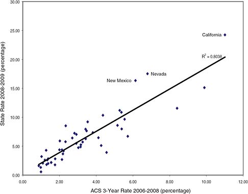
FIGURE 5-1 Comparison of ACS 3-year rate and state-provided rate of all ELL students for the 2008-2009 school year.
Figures 5-1 and 5-2). The rate based on the tested, not proficient count for Alaska is also considerably higher than the ACS estimate (see Figure 5-2).
We investigated several state-specific factors that might help to explain discrepancies between ACS estimates and state-provided counts, including demographic variables and testing practices.
Demographic Factors
We focused on demographic variables that represent characteristics of immigrant populations that might affect the differences between the state-provided counts and ACS estimates of ELL rates. We considered (1) the percentage of school-age immigrant children in the state, (2) the percentage of unauthorized immigrants in the state (Passel et al., 2006), (3) the percentage of unauthorized Mexicans in the state (Passel et al., 2006), (4) the percentage of foreign-born residents in the state with incomes below the poverty level, and (5) an indicator variable for states with large percentages of unauthorized immigrants (Arizona, California, New Mexico, Nevada, Texas).
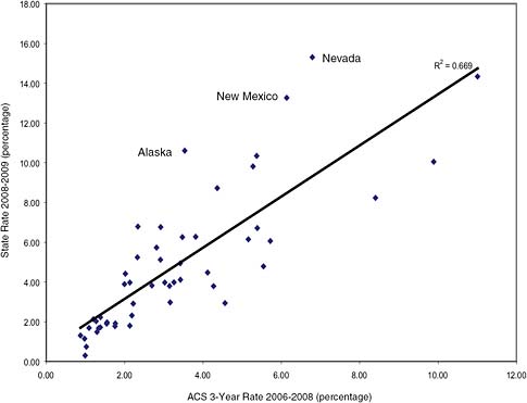
FIGURE 5-2 Comparison of ACS 3-year rate and state-provided rate of tested, not proficient students for the 2008-2009 school year.
These variables capture a number of hypothetical mechanisms. For example, unauthorized immigrants may be undercovered in the ACS although their schoolage children would appear in the state counts. For another example, some groups of immigrant parents may overestimate the English speaking skills of their children relative to their own limited skills or by comparing them to requirements for community and family interactions rather than academic settings, particularly if their own formal education is limited.
State Practices
As discussed in Chapters 3 and 4, states use different tests, procedures, and criteria for classifying and reclassifying ELL students and for exiting them from programs. These differences might contribute to differential discrepancies between ACS estimates and state counts. It is difficult, however, to quantify the characteristics of state procedures, which are too complex and multidimensional to lend themselves to a simple rank ordering by stringency. Procedures also vary across districts in some states.
In the analyses shown in Tables 5-7 and 5-8, the dependent variable was the rate based on the state-provided count, and the ACS 3-year estimate was included as an explanatory variable, along with the other variables intended to test our hypotheses. Table 5-7 shows the results of the regressions for analyses in which the dependent variable was the rate based on the state-provided count of all ELL students. Table 5-8 shows the results when the dependent variable was based on the state-provided count of tested, not proficient students.
We ran nine different models for each year of state data (2007-2008 and 2008-2009). Model 1, the baseline model, included the 3-year ACS estimate as the only predictor of the state counts.2 As shown in Table 5-7, the R2 (the fraction of variance in state-provided rates explained by the predictor variable) for this model, when the rate of all ELL students was the dependent variable, was 0.73 for 2007-2008 and 0.80 for 2008-2009. Similarly, Table 5-8 shows that the R2 for the basic model (Model 1), when the dependent variable was the rate of tested, not proficient students, was 0.66 for 2007-2008 and 0.66 for 2008-2009.3
Each of the successive models (2 through 9) added explanatory variables to examine the extent to which prediction of the state-provided counts might be improved. Models 2 through 7 included the variables intended to serve as proxies for the effects of the composition of the immigrant population in the state. Of these variables, only two were statistically significant predictors: the indicator variable for states (Arizona, California, New Mexico, Nevada, and Texas) with a high percentage of unauthorized immigrants (Table 5-7, Model 6, both years; Table 5-8, Model 6, 2007-2008) and the percentage of unauthorized Mexican immigrants (Table 5-8, Model 5, 2007-2008). The size and direction of the coefficients suggest that the ACS slightly underestimates the state-provided rate in states with high percentages of unauthorized immigrants (Table 5-7, Model 6, both years; Table 5-8, Model 6, 2007-2008). These findings provide some support for our hypothesis about the effects of the unauthorized immigrant population on the differences between the state counts and ACS estimates.
Models 8 and 9 both included indicators for states that used the ACCESS test (N, 18) or the ELDA test (N, 6). Neither of these indicators was a statistically significant predictor. We conducted one follow-up analysis, focused solely on the states that use the ACCESS test (the largest group in the country that uses the same test). As described in Chapter 3, states that use the ACCESS test are allowed to determine the specific proficiency level needed for ELL students to be exited from ELL classification. The ACCESS reports scores using six proficiency levels, and most states require students to score at least at the fourth level in order to be exited from the classification. However, some require students to score at the fifth level, some require students to score at the sixth level, and some specify additional criteria for the subtest scores. We attempted to classify states according to the stringency of their require-
TABLE 5-7 Analysis of Using ACS 3-Year Estimate and Other Variables to Predict State-Provided Rate of All ELL Students
|
|
|
2007-2008 |
2008-2009 |
|
Model 1 |
Adjusted R2 |
.73** |
.80** |
|
|
Regression Coefficients (Standard Error): |
|
|
|
|
ACS 2006-2008 |
1.669** (.1449) |
1.8305 (.1292)** |
|
|
Intercept |
.0075 (.0054) |
.0024 (.0052) |
|
Model 2 |
Adjusted R2 |
.73** |
.79** |
|
|
Regression Coefficients (Standard Error): |
|
|
|
|
ACS 2006-2008 |
1.6580 (.1949)** |
1.9061 (.1754)** |
|
|
Percent immigrants |
.0760 (.9245) |
–.5845 (.9104) |
|
|
Intercept |
.0073 (.0060) |
.0042 (.0060) |
|
Model 3 |
Adjusted R2 |
.73** |
.80** |
|
|
Regression Coefficients (Standard Error): |
|
|
|
|
ACS 2006-2008 |
1.5330 (.4709)** |
1.5345 (.4600)** |
|
|
Percent immigrants in poverty |
.4413 (1.4583) |
.9884 (1.4734) |
|
|
Intercept |
.0077 (.0055) |
.0028 (.0052) |
|
Model 4 |
Adjusted R2 |
.72** |
.80** |
|
|
Regression Coefficients (Standard Error): |
|
|
|
|
ACS 2006-2008 |
1.8110 (.3496)** |
1.4574 (.2919)** |
|
|
Percent unauthorized immigrants |
–.1358 (.5039) |
.5911 (.4157) |
|
|
Intercept |
.0060 (.0061) |
.0040(.0053) |
|
Model 5 |
Adjusted R2 |
.74** |
.82** |
|
|
Regression Coefficients (Standard Error): |
|
|
|
|
ACS 2006-2008 |
1.4188 (.2432)** |
1.4006 (.2118)** |
|
|
Percent unauthorized Mexicans |
.7505 (.4617) |
.9901 (.3973)* |
|
|
Intercept |
.0096 (.0062) |
.0075 (.0053) |
|
Model 6 |
Adjusted R2 |
.75** |
.82** |
|
|
Regression Coefficients (Standard Error): |
|
|
|
|
ACS 2006-2008 |
1.3943 (.2126)** |
1.5047 (.1891)** |
|
|
States with high percent unauthorized |
.0350 (.0161)* |
.0323 (.0142)* |
|
|
Intercept |
.0141 (.0068)* |
.0102 (.0060) |
|
Model 7 |
Adjusted R2 |
.75** |
.82** |
|
|
Regression Coefficients (Standard Error): |
|
|
|
|
ACS 2006-2008 |
1.3241 (.2483)** |
1.3282 (.2195)** |
|
|
Percent unauthorized Mexican |
.3040 (.5449) |
.7059 (.4622) |
|
|
States with high percent unauthorized |
.0290 (.0194) |
.0194 (.0163) |
|
|
Intercept |
.0141 (.0068)* |
.0107 (.0059) |
|
Model 8 |
Adjusted R2 |
.73** |
.79** |
|
|
Regression Coefficients (Standard Error): |
|
|
|
|
ACS 2006-2008 |
1.5814 (.1590)** |
1.7979 (.1456)** |
|
|
ACCESS user |
–.0078 (.0069) |
–.0029 (.0069) |
|
|
ELDA user |
–.0097 (.0090) |
–.0042 (.0095) |
|
|
Intercept |
.0140 (.0073) |
.0052 (.0074) |
|
|
|
2007-2008 |
2008-2009 |
|
Model 9 |
Adjusted R2 |
.72** |
.79** |
|
|
Regression Coefficients (Standard Error): |
|
|
|
|
ACS 2006-2008 |
1.4786 (.4945)** |
1.5912 (.4832)** |
|
|
Percent immigrants |
–.1681 (.9603) |
–.7492 (.9595) |
|
|
Percent immigrants in poverty |
.4046 (1.4826) |
.9851 (1.5130) |
|
|
ACCESS user |
–.0801 (.0071) |
–.0035 (.0070) |
|
|
ELDA user |
–.0010 (.0095) |
–.0056 (.0099) |
|
|
Intercept |
.0148 (.0082) |
.0084 (.0085) |
|
NOTES: * p < .05; **p < .01. All R2 values were adjusted for the sample size (n = 51). |
|||
ments on the ACCESS test. We then ran a regression on just these 18 states to see if the relationship between state counts and ACS estimates was improved when the stringency of ACCESS proficiency requirements was considered. The results did not support this hypothesis: no improvement in R2 was evident when the stringency of proficiency requirements was considered.
We also ran a series of analyses to investigate the effects of changing the ACS cut score on the relationship between ACS estimates and state counts. For these analyses, we classified students as ELL students if their parents indicated their English speaking skills were “less than well” (rather than “less than very well”). We then examined the relationships between ACS estimates and state counts. The results showed no improvement in the relationships between ACS estimates and state counts: in fact, the percent of variance explained generally declined.4 We also tried including ratios at all of the cut points in the same model: we found that those below the “less than very well” cut point were not significant predictors.
CONCLUSION 5-2 On the basis of the analysis of the effect of the American Community Survey (ACS) cut-point on the relationship between the ACS estimates and the state counts, the cut point of “less than very well”
|
4 |
Two models were run. In the first, the dependent variable was the state provided count of ELL students divided by all public school enrollees for the 2007-2008 school year. The independent variable was the ACS 2006-2008 estimate of youths aged 5-18 years enrolled in public school enrolled who spoke English “less than well” divided by youths aged 5-18 years enrolled in public school. The adjusted R-square was 0.49 and the ACS variable was significant at 0.01 level. In the second model, the dependent variable was the state-provided count of tested, not proficient ELL students divided by all public school students enrolled for the 2007-2008 school year. The independent variable was the ACS 2006-2008 estimate of youths aged 5-18 years enrolled in public school who spoke English “less than well” divided by 5-18 years old and enrolled in public school. The adjusted R-square was 0.38, and the ACS variable was significant at the 1% level. Thus, even though the “less than well” variable was significant, its t-value was much lower than the “less than very well” variable in Model 1 in Tables 5-7 and 5-8. Also, both of these models had much lower explanatory power relative to the model with “less than very well” as the explanatory variable. |
TABLE 5-8 Analysis of Using ACS 3-Year Estimate and Other Variables to Predict State-Provided Rate of Tested, Not Proficient ELL Students
|
|
|
2007-2008 |
2008-2009 |
|
Model 1 |
Adjusted R2 |
.66** |
.66** |
|
|
Regression Coefficients (Standard Error): |
|
|
|
|
ACS 2006-2008 |
1.300** (.1300) |
1.2871 (.1293)** |
|
|
Intercept |
.0034 (.0052) |
.0057 (.0051) |
|
Model 2 |
Adjusted R2 |
.66** |
.66** |
|
|
Regression Coefficients (Standard Error): |
|
|
|
|
ACS 2006-2008 |
1.320 (.1773)** |
1.2752 (.1763)** |
|
|
Percent immigrants |
–0.1566 (.920) |
.0918 (.9152) |
|
|
Intercept |
.0039 (.0060) |
.0052 (.0062) |
|
Model 3 |
Adjusted R2 |
.67** |
.66* |
|
|
Regression Coefficients (Standard Error): |
|
|
|
|
ACS 2006-2008 |
0.8173 (.4597) |
1.0598 (.4614)* |
|
|
Percent immigrants in poverty |
1.612 (1.4722) |
.7589 (1.4778) |
|
|
Intercept |
.0040 (.0052) |
.0060 (.0053) |
|
Model 4 |
Adjusted R2 |
.67** |
.66* |
|
|
Regression Coefficients (Standard Error): |
|
|
|
|
ACS 2006-2008 |
0.9594 (.2950)** |
0.9758(.2941)** |
|
|
Percent unauthorized immigrants |
0.5396 (.4201) |
.4930 (.4188) |
|
|
Intercept |
.0049 (.0053) |
.0071(.0053) |
|
Model 5 |
Adjusted R2 |
.71** |
.68** |
|
|
Regression Coefficients (Standard Error): |
|
|
|
|
ACS 2006-2008 |
0.8221 (.2102)** |
0.9773 (.2185)** |
|
|
Percent unauthorized Mexicans |
1.1009 (.3943)** |
.7134 (.4099) |
|
|
Intercept |
.0090 (.0053)* |
.0094 (.0055) |
|
Model 6 |
Adjusted R2 |
.70** |
.67** |
|
|
Regression Coefficients (Standard Error): |
|
|
|
|
ACS 2006-2008 |
0.9105 (.1862)** |
1.0807 (.1954)** |
|
|
States with high percent unauthorized |
.0387 (.0140)** |
.0205 (.0146) |
|
|
Intercept |
.0127 (.0059)* |
.0107 (.0062)* |
|
Model 7 |
Adjusted R2 |
.71** |
.67** |
|
|
Regression Coefficients (Standard Error): |
|
|
|
|
ACS 2006-2008 |
0.7279 (.2154)** |
0.9395 (.2290)** |
|
|
Percent unauthorized Mexican |
.7306 (.4537) |
.5649 (.4822) |
|
|
States with high percent unauthorized |
.0253 (.0160) |
.0102 (.0170) |
|
|
Intercept |
.0132 (.0058)* |
.0110 (.0062) |
|
Model 8 |
Adjusted R2 |
.66** |
.66** |
|
|
Regression Coefficients (Standard Error): |
|
|
|
|
ACS 2006-2008 |
1.2327(.1449)** |
1.2208 (.1444)** |
|
|
ACCESS user |
–.0080(.0068) |
–.0067 (.0067) |
|
|
ELDA user |
–.0056 (.0095) |
–.0074 (.0094) |
|
|
Intercept |
.0093 (.0074) |
.0114 (.0074) |
|
|
|
2007-2008 |
2008-2009 |
|
Model 9 |
Adjusted R2 |
.65** |
.64** |
|
|
Regression Coefficients (Standard Error): |
|
|
|
|
ACS 2006-2008 |
0.7988 (.4795) |
1.0263 (.4833)* |
|
|
Percent immigrants |
–.3598 (.9523) |
–.1165 (.9598) |
|
|
Percent immigrants in poverty |
1.5989 (1.5016) |
.6992 (1.5134) |
|
|
ACCESS user |
–.0083 (.0070) |
–.0068 (.0070) |
|
|
ELDA user |
–.0057 (.0098) |
–.0074 (.0099) |
|
|
Intercept |
.0111 (.0084) |
.0120 (.0084) |
|
NOTES: *p < .05; **p < .01. All R2 values were adjusted for the sample size (n = 51). |
|||
on the ACS language item appears to best approximate school assessments of English language learner status.
It should be noted that the small number of units (50 states and the District of Columbia) limited the number of variables that could be considered. Furthermore, the concentration of ELL populations in relatively few states further limited our ability to infer systematic correlates of the discrepancies between the data sources.
Within-State Analyses
We also conducted a series of regression analyses to examine the relationships between ACS estimates and state-provided counts for school districts (local education agencies or LEAs) within each state. The purpose of this analysis was to assess how well the ACS and state-provided numbers tracked each other under a consistent set of procedures, criteria, and tests, that is, those of a single state. We obtained the 3-year (2006-2008) ACS estimates and the state-provided (2007-2008) counts of all ELL students for each unified school district for which they were available, which limited us to school districts with total populations of at least 20,000 (due to ACS release restrictions for small areas). Also excluded were several states for which LEA-level data were unavailable (California, New Jersey, and South Dakota). This analysis could be conducted only with rates based on state counts of all ELL students, since LEA counts of tested, not proficient students were not available. We formed the rate for each district (that is, we divided each of the counts by the number of K-12 students enrolled in public schools in the state).
For smaller units of analyses, such as most school districts, the sampling variability of ACS estimates of rates is generally greater than for states. Simple sample correlations would be attenuated by this error, underestimating the strength of the underlying relationship between the ACS and state-provided measures. We therefore used hierarchical models that adjust for the sampling variability of the ACS data to estimate this relationship. For these analyses, the dependent variable was the ACS
estimate of the school district’s ELL rate, and the explanatory variable was the state-provided estimate of the district rate. (Making the ACS rate the dependent variable facilitated specification of a hierarchical model in which the difference between the ACS estimate and its linear prediction from the state-reported rate is modeled as the sum of two random effects, one for ACS sampling error with known variance, and one for the discrepancy between the ACS and the state rate with variance to be estimated.)
Table 5-9 shows descriptive information for each of the states included in the analysis. The first two columns show the school enrollment and the number of unified districts in the state. The third column shows the overall rate of ELL students in the state based on state-provided information. The next three columns provide distributional information about the LEA rates within the state (based on the state-provided information): the average rate across the districts and the 20th and 80th percentiles of the LEA rates in the state. The seventh column shows the overall rate of ELL students in the state based on the ACS information. The eighth column presents the ratio of the ACS rate to the state-provided rate. The final column shows the sample correlation of the rates based on ACS estimates and state-provided counts for the unified school districts within a state. For instance, the correlation between the two sets of rates for the 58 unified school districts in Alabama was 0.697. The correlation is labeled “unadjusted” because it has not been corrected for sampling error associated with the ACS estimates.
Table 5-10 presents the results of the within-state regressions in states with at least 10 eligible LEA units, incorporating a correction for sampling error in the ACS estimates. The first four columns show the results from regressions that include the intercept in the model. The first two columns show, respectively, the regression coefficients for the intercept and for the rate based on the state-provided estimate. The third column shows the root mean square residual error (RMSE) of the model, which quantifies the amount by which the ACS estimates by LEA vary around the regression line. The fourth column shows the correlations after adjustment for sampling error. The median of these estimated correlation coefficients is 0.949, and the coefficient exceeds 0.90 in 30 of 41 states, although there are also a few states for which these LEA-level correlations are relatively low.
The fifth and sixth columns show parallel results (regression coefficients and RMSE) from the regressions that did not include the intercept in the model. The final column is the ratio of the errors from the two models (with and without intercepts). This ratio is usually not far from 1.0 (except in a few states where the denominator is very small due to an extremely good model fit), suggesting that the no-intercept (proportional) model fits the data almost as well as the unconstrained linear model. As noted previously, the proportional model implies that ACS-based and state-data-based allocations would be equivalent.
In general, the results suggest very good consistency between the ACS and state-provided numbers within states. This greater consistency, relative to similar models fitted at the state level, might be attributed to two features of the within-
TABLE 5-9 Descriptive Summaries of LEA-Level Data on Rate of ELL Students, by State
|
|
State Counts |
State ELL Rates |
ACS Overall Rate (%) |
Ratio of ACS/State |
Unadjusted Correlation |
||||
|
State |
School Enrollment |
Number of LEAs |
Overall Rate (%) |
Mean of LEAs (%) |
20%-tile (%) |
80%-tile (%) |
|||
|
Alabama |
579,913 |
58 |
3.0 |
2.8 |
0.4 |
4.7 |
1.3 |
0.44 |
0.697 |
|
Alaska |
93,838 |
5 |
7.4 |
5.8 |
2.4 |
10.6 |
2.6 |
0.34 |
0.207 |
|
Arizona |
872,395 |
72 |
14.2 |
14.5 |
3.7 |
26.2 |
9.6 |
0.68 |
0.798 |
|
Arkansas |
227,292 |
30 |
8.7 |
5.9 |
0.6 |
7.3 |
3.1 |
0.36 |
0.918 |
|
Colorado |
684,657 |
35 |
11.3 |
11.9 |
2.5 |
21.4 |
5.8 |
0.51 |
0.920 |
|
Connecticut |
378,744 |
56 |
7.3 |
5.3 |
1.4 |
10.1 |
3.9 |
0.54 |
0.877 |
|
Delaware |
102,396 |
13 |
6.7 |
5.8 |
2.1 |
9.0 |
3.3 |
0.49 |
0.529 |
|
District of Columbia |
57,877 |
1 |
7.1 |
7.1 |
7.1 |
7.1 |
2.3 |
0.33 |
NA |
|
Florida |
2,619,362 |
54 |
8.8 |
5.2 |
0.9 |
9.4 |
5.2 |
0.59 |
0.682 |
|
Georgia |
1,487,247 |
97 |
5.2 |
3.5 |
0.7 |
5.4 |
3.3 |
0.64 |
0.885 |
|
Hawaii |
179,897 |
1 |
10.4 |
10.4 |
10.4 |
10.4 |
4.4 |
0.42 |
NA |
|
Idaho |
180,200 |
20 |
5.2 |
5.5 |
0.3 |
11.3 |
2.4 |
0.46 |
0.904 |
|
Illinois |
1,519,448 |
202 |
11.4 |
7.2 |
0.8 |
10.6 |
6.4 |
0.56 |
0.769 |
|
Indiana |
705,862 |
87 |
5.5 |
4.9 |
1.0 |
7.5 |
2.4 |
0.44 |
0.776 |
|
Iowa |
220,538 |
29 |
6.0 |
4.8 |
0.8 |
7.2 |
2.5 |
0.42 |
0.646 |
|
Kansas |
272,573 |
28 |
9.6 |
9.2 |
1.6 |
12.9 |
4.1 |
0.42 |
0.907 |
|
Kentucky |
463,556 |
54 |
2.4 |
1.4 |
0.2 |
1.8 |
1.6 |
0.67 |
0.647 |
|
Louisiana |
606,547 |
49 |
1.8 |
1.2 |
0.1 |
1.6 |
1.4 |
0.76 |
0.418 |
|
Maine |
45,917 |
12 |
5.8 |
4.3 |
0.4 |
6.3 |
3.7 |
0.63 |
0.797 |
|
Maryland |
843,426 |
23 |
4.8 |
2.6 |
0.6 |
3.4 |
3.0 |
0.63 |
0.862 |
|
Massachusetts |
639,309 |
110 |
8.1 |
4.8 |
0.6 |
9.3 |
5.3 |
0.65 |
0.819 |
|
Michigan |
830,996 |
103 |
4.6 |
3.5 |
0.4 |
5.1 |
2.6 |
0.55 |
0.718 |
|
Minnesota |
537,291 |
60 |
9.2 |
6.5 |
1.3 |
10.1 |
4.7 |
0.51 |
0.779 |
|
Mississippi |
300,235 |
44 |
1.4 |
1.4 |
0.3 |
2.1 |
1.0 |
0.71 |
0.069 |
TABLE 5-10 Results of Within-State Regressions
|
|
Model with Intercept, State Data Rate |
No-Intercept Model |
Number of LEAs |
Ratio of RMSE Estimates |
||||
|
|
Intercept Coefficient |
State Coefficient |
RMSE |
Adjusted Correlation |
State Coefficient |
RMSE |
||
|
Alabama |
0.0026 |
0.2508 |
0.0036 |
0.9040 |
0.3084 |
0.0033 |
58 |
0.93 |
|
Arizona |
0.0216 |
0.3852 |
0.0316 |
0.8433 |
0.4765 |
0.0346 |
72 |
1.09 |
|
Arkansas |
0.0049 |
0.2747 |
0.0003 |
0.9999 |
0.3099 |
0.0003 |
30 |
1.11 |
|
Colorado |
0.0029 |
0.4477 |
0.0004 |
1.0000 |
0.4693 |
0.0013 |
35 |
3.20 |
|
Connecticut |
0.0043 |
0.4038 |
0.0065 |
0.9596 |
0.4602 |
0.0067 |
56 |
1.03 |
|
Delaware |
0.0171 |
0.1587 |
0.0027 |
0.8904 |
0.3816 |
0.0069 |
13 |
2.56 |
|
Florida |
0.0073 |
0.4762 |
0.0127 |
0.8737 |
0.5540 |
0.0134 |
54 |
1.06 |
|
Georgia |
0.0044 |
0.5006 |
0.0043 |
0.9814 |
0.5723 |
0.0048 |
97 |
1.13 |
|
Idaho |
0.0053 |
0.3292 |
0.0005 |
0.9997 |
0.3958 |
0.0036 |
20 |
7.73 |
|
Illinois |
0.0139 |
0.3808 |
0.0189 |
0.8834 |
0.4739 |
0.0220 |
202 |
1.17 |
|
Indiana |
0.0034 |
0.2750 |
0.0035 |
0.9778 |
0.3224 |
0.0033 |
87 |
0.92 |
|
Iowa |
0.0095 |
0.1688 |
0.0066 |
0.8514 |
0.2623 |
0.0096 |
29 |
1.46 |
|
Kansas |
0.0017 |
0.3394 |
0.0102 |
0.9675 |
0.3508 |
0.0102 |
28 |
1.00 |
|
Kentucky |
0.0046 |
0.4069 |
0.0033 |
0.9360 |
0.5251 |
0.0021 |
54 |
0.65 |
|
Louisiana |
0.0061 |
0.2929 |
0.0020 |
0.9192 |
0.4801 |
0.0047 |
49 |
2.38 |
|
Maine |
0.0037 |
0.3091 |
0.0054 |
0.9590 |
0.3769 |
0.0043 |
12 |
0.79 |
|
Maryland |
0.0049 |
0.4777 |
0.0067 |
0.8872 |
0.5681 |
0.0074 |
23 |
1.11 |
|
Massachusetts |
0.0064 |
0.4551 |
0.0042 |
0.9891 |
0.5173 |
0.0047 |
110 |
1.11 |
|
Michigan |
0.0075 |
0.2692 |
0.0052 |
0.9318 |
0.3665 |
0.0068 |
103 |
1.31 |
|
Minnesota |
0.0092 |
0.3170 |
0.0107 |
0.9038 |
0.3984 |
0.0123 |
60 |
1.16 |
|
Mississippi |
0.0051 |
0.0874 |
0.0024 |
0.6004 |
0.2673 |
0.0001 |
44 |
0.04 |
|
Missouri |
0.0068 |
0.3750 |
0.0019 |
0.9820 |
0.5429 |
0.0038 |
65 |
2.04 |
|
Montana |
0.0045 |
0.1244 |
0.0013 |
0.8678 |
0.2576 |
0.0038 |
15 |
2.91 |
|
Nebraska |
0.0081 |
0.3081 |
0.0006 |
0.9996 |
0.3758 |
0.0063 |
15 |
10.44 |
state comparison: (1) the use of consistent procedures and criteria within most states but different ones in different states, and (2) the possibly greater similarity among immigrant populations within the same state than those in different states. The first of these reasons points to the difficulties in making present state-provided data comparable across states, while the second indicates possible difficulties in interstate comparability for ACS data. Nonetheless, the high degree of within-state consistency does give some reason for optimism that better consistency is achievable.
CONCLUSION 5-3 In the absence of other factors, such as the legislated minimum allocation, the American Community Survey and state-provided data would yield broadly similar allocations to most states. However, the differences in allocations to a few states are substantial and not readily explainable by such factors as region of the country, demographic characteristics of the English language learner population, or the proficiency test used by the state.
Temporal Variation
Another criterion for comparison of the ACS estimates and state counts is the degree of variation over time of the estimates for each state. There are conflicting values in consideration of such variation. Responsiveness refers to the tendency of a set of estimates to respond quickly to changes in conditions, such as rapid growth of the population of immigrant children in a state from one year to the next. This term suggests a positive value in that resources will be more rapidly directed to states with growing needs if a more responsive measure is used. Volatility refers to the tendency of estimates to vary or fluctuate from year to year. It suggests a negative value since such funding fluctuations make it more difficult to plan and maintain program continuity. Responsiveness contributes directly to volatility when populations are changing, but there are additional sources of volatility particular to each data source. Sampling variation contributes to purely random volatility in the ACS estimates. State data could become volatile when a state changes its tests, standards, or procedures from one year to the next or when there is an error or change in the mechanisms for reporting ELL counts from school districts to states to the DoEd.
Table 5-11 summarizes the volatility of ACS and state-provided estimates of ELL counts in two ways (parallel to those used in the sensitivity analyses in Chapter 2). The first is the sum of absolute changes in state shares, equivalent to twice the portion of the total allocation that would be moved from one state to another in consecutive years. The second is the mean absolute value of relative changes in shares, which summarizes the amount by which allocations in each state change relative to the size of its allocation. As expected, the single-year ACS changes are about equal in the two pairs of years (2006 to 2007 and 2007 to 2008). As explained in Chapter 2, the 3-year ACS estimates are much more stable, both because of the greater reliability of 3 years of data and because only one out of the years changes in overlapping
TABLE 5-11 Comparison of Volatility in ACS Estimates and State-Provided Counts (in percentage)
3-year periods. (For the same reason, these estimates are also the least responsive.) Interestingly, the between-year changes in state-provided shares are much larger in 2006-2007 than in 2007-2008. We do not have enough detailed information about changes in state practices to identify specific reasons for the changes that might cause this variation and predict whether results would be similar in future years.
The more detailed information by state share grouping sheds more light on patterns of volatility. In absolute terms, the largest part of annual changes in share occurs in the states with relatively large shares; as noted above, these encompass about 74 percent of allocations. However in relative terms, these states show the least volatility by any measure. Since volatility in ACS estimates is largely driven by sampling variation, it is consistently larger in relative terms for each group of successively smaller states. The pattern is less consistent in the state-provided estimates, although generally the larger states tend to have more stable numbers. This stability may reflect the greater effects on smaller states of rapid changes in ELL population in a few local areas, or it may reflect changes in reporting. Overall, the 3-year ACS estimates appear to be the most stable, at the cost of some loss of responsiveness. And as discussed in Chapter 2, 1-year ACS estimates do not capture year-to-year changes with acceptable precision. The evidence is ambiguous on comparative stability of single-year ACS estimates and state-based estimates.
CONCLUSION 5-4 The superior precision and stability of the 3-year American Community Survey (ACS) estimates outweigh their slower responsiveness to changes and make them superior to the ACS 1-year estimates as a basis for allocations.


