Below are the first 10 and last 10 pages of uncorrected machine-read text (when available) of this chapter, followed by the top 30 algorithmically extracted key phrases from the chapter as a whole.
Intended to provide our own search engines and external engines with highly rich, chapter-representative searchable text on the opening pages of each chapter. Because it is UNCORRECTED material, please consider the following text as a useful but insufficient proxy for the authoritative book pages.

Do not use for reproduction, copying, pasting, or reading; exclusively for search engines.

OCR for page 28
3 Lessons Learned from Ocean Color Satellite Missions and Essential Requirements for Future Success B THE COASTAL ZONE COLOR SCANNER: uilding and launching a sensor are only the first PROOF OF CONCEPT steps toward successfully producing ocean color radiance and ocean color products. Even if the sen- CZCS was the first ocean color sensor to provide local- sor meets all high-quality requirements, without stability to global-scale ocean color observations during its operation monitoring, vicarious calibration, and reprocessing capa - from 1978 to 1986 (Hovis et al., 1980; Gordon and Morel, bilities, the data will not meet standards for scientific and 1983). CZCS was launched on Nimbus 7 and was a prototype climate-impact assessments. This chapter surveys lessons mission to demonstrate that ocean color can be retrieved from from previous missions and outlines the requirements for space. Therefore, CZCS did not routinely or continuously obtaining useful ocean color data from a global remote collect global data because it had to share power and tape sensing mission. recorder capacity with other sensors. During the past three decades, several polar orbiting The quality of CZCS data products was significantly satellites have been launched to measure water-leaving compromised by the lack of a sustained in situ monitoring radiance (Lw) on a global scale approximately every one program of Lw to provide sea-truth for the satellite mea- to three days (depending primarily on swath width; see surements, and by the lack of near-infrared wavebands for Appendix A for a detailed satellite description). The pro - atmospheric correction (Evans and Gordon, 1994). During gression from the Coastal Zone Color Scanner (CZCS) to the initial phase of CZCS, NASA and the Nimbus Experi- the Sea-viewing Wide Field-of-view Sensor (SeaWiFS), ment Team supported a well-formulated program of in situ to the Moderate Resolution Imaging Spectroradiometer observations. These data were key in providing the initial (MODIS), and finally to the Joint Polar Satellite System instrument vicarious calibration; however, the program was (JPSS) Visible Infrared Imager Radiometer Suite (VIIRS), active only during the first months of CZCS on-orbit lifetime represents the progression from pilot study to research (Werdell et al., 2007). Because CZCS experienced significant to operational ocean color remote sensing for the United degradation of the green and blue bands over its lifetime, and States. With the exception of the most recent European the red band used for atmospheric correction experienced Medium-Resolution Imaging Spectrometer (MERIS) mis - an abrupt shift in its performance, CZCS calibration relied sion, each of these satellite missions carried a Type 1 (see heavily on clear water assumptions for the green bands and Table 2.1) sensor with only moderate spatial and spectral other simplifying assumptions that could not be validated resolution. The planned Pre-Aerosol-Clouds-Ecosystem (Evans and Gordon, 1994). Further, sampling by CZCS was (PACE) mission outlined in the National Aeronautics and not global and except for regions where data were routinely Space Administration’s (NASA) Climate Architecture Plan collected such as the coastal United States, special requests (2010) represents an advanced Type 1 ocean color research were necessary to initiate data acquisition. In fact, no mission. Therefore, this retrospective analysis is restricted CZCS observations were ever made in large regions of the to Type 1 sensors. Although some conclusions and recom - global ocean, such as in the South Pacific Subtropical Gyre. mendations are specific to Type 1 missions, many lessons Limitations in sensor performance and the lack of sustained, about mission design and requirements apply to all sensor continuous global observations restricted CZCS’s ability to types. quantify long-term changes in the global ocean biosphere. However, the need for continuous vicarious calibration was 28

OCR for page 28
29 LESSONS LEARNED FROM OCEAN COLOR SATELLITE MISSIONS recognized and led to the Marine Optical Buoy (MOBY) 2011). Relative calibration coefficients for some bands had system. decreased by as much as nearly 20 percent (Figure 3.4); however, uncertainty about the fit trend lines for the lunar Conclusion: During the CZCS era, scientists learned about views were quite small (~0.1 percent for all bands). Second, uncertainties in the MOBY water-leaving radiances (Lw(λ)) the importance of continuous sampling to achieve global coverage, of making in situ measurements throughout involve both the MOBY spectrometer calibration and the a mission’s lifetime to assess changes in the sensor’s propagation of the subsurface radiances through the water gain over time and to validate the data products, and of column and the air-sea interface. Brown et al. (2007) provide the contribution of each to the Lw(λ) error budget, with the atmospheric corrections. In particular, the need for near- total uncertainty in Lw(λ) ranging from 2.1 to 3.3 percent infrared (NIR) measurements to improve atmospheric cor- depending on the spectral band. The Lw(λ) contribution to rection was recognized during the CZCS experience and led to the SeaWiFS band-set. the top of the atmosphere radiance is typically 10 percent for oligotrophic waters and clear atmospheres, which are typically found where MOBY has been deployed. Thus the LESSONS FROM THE SEAWIFS/MODIS ERA Lw(λ) uncertainty is equivalent to 0.21 to 0.33 percent at the SeaWiFS and MODIS-Aqua have been highly success- top of the atmosphere. Third, uncertainties in the vicarious ful, global-scale U.S. ocean color missions that contributed calibration of gain factors for individual time points were to major advances in the ocean sciences (Siegel et al., 2004; often large (~1 percent; Franz et al., 2007) and are primarily NRC, 2008a; McClain, 2009). SeaWiFS launched in Sep- due to uncertainty in the atmospheric corrections (Gordon, tember 1997 with a design life of five years and operated 1997; Ahmad et al., 2010). After evaluating many (>50) for 13 years, until December 14, 2010 (Hooker et al., 1992; independent estimates, the uncertainty in the mean gains McClain, 2009). SeaWiFS provided almost daily global (standard errors about the mean) are ~0.1 percent (Table 1 Earth coverage from a polar orbit. Six visible bands detected in Franz et al., 2007). It is interesting to note that the largest changes in ocean properties with high signal-to-noise ratio source of uncertainty to the SeaWiFS calibration budget is (SNR) to allow discrimination of low ocean reflectance from the vicarious calibration source used. against a very high atmospheric background signal. Two In December 1999, MODIS followed SeaWiFS on the near-infrared (NIR) bands were used to estimate aerosol Earth Observing System (EOS) Terra spacecraft and in May properties for atmospheric correction (although reduction in 2002, on EOS Aqua. Each had a design life of five years digitization of the NIR channels was an important source of (Esaias et al., 1998). Both remain operational after 11 and 8 noise in open ocean retrievals [Hu et al., 2004]). Key design years on-orbit, respectively. MODIS addresses atmosphere, features minimized polarization sensitivity and far-field stray land, and ocean research requirements; the Aqua sensor light and enabled the measurement of low signal ocean radi- continues SeaWiFS ocean color capability. ances, and land and cloud reflectance at very high signals, Unfortunately, the Terra MODIS sensor has major without saturation. A solar diffuser assisted with the on-orbit limitations in its application of ocean color products because sensor performance evaluation (Eplee et al., 2007). The sen- of poor radiometric and polarization stability (Franz et al., sor tilt capability minimized sun glint. Most importantly, 2008). The recent reprocessing of Terra MODIS (January the lunar calibration capability (Barnes et al., 2004) helped 2011) was only possible because the entire dataset was SeaWiFS achieve superb long-term stability. vicariously calibrated using SeaWiFS observations. These The overall uncertainty level for SeaWiFS calibration difficulties with Terra MODIS highlight the need for a stable gains can be estimated to be ~0.3 percent (assuming indepen- and well-characterized ocean color sensor. dence among the three sources of uncertainty). Reducing the Nine of 36 MODIS spectral bands are within the vis- system calibration uncertainty to such a low number was a ible range matching SeaWiFS, with the exception of slight major accomplishment of the SeaWiFS mission and resulted c hanges in bandpass (see below). The MODIS sensor from a commitment to minimizing the sources of uncertainty includes for the first time spectral bands that detect the chlo- from three primary independent sources: (1) uncertainty in rophyll fluorescence line height from satellite orbit (Letelier the calibration trends in time, (2) uncertainty in the MOBY and Abbott, 1996; Behrenfeld et al., 2009). Like SeaWiFS, calibration and its determinations of water-leaving radiance, MODIS is able to measure the low-signal radiance from the and (3) uncertainty in the estimation of SeaWiFS calibration ocean as well as the high-signal reflectance from land and gain corrections. The details of the three sources of uncer- clouds throughout the visible and near-infrared. Therefore, tainty are presented below; however, their contribution to MODIS provides full atmosphere, land, and ocean spectral estimation of the overall uncertainty levels are briefly dis- and radiometric coverage for a broad range of applications, cussed here. First, uncertainty in the estimation of SeaWiFS including ocean color. Moreover, MODIS improves Sea- calibration over time, i.e., sensor sensitivity degradation, WiFS calibration with a better solar diffuser, a solar diffuser has been determined for SeaWiFS using its monthly lunar stability monitor to compensate for solar diffuser changes viewing of the moon at the same phase (Eplee et al., 2004, over time, and a spectroradiometric calibration assembly that

OCR for page 28
30 SUSTAINED OCEAN COLOR RESEARCH AND OPERATIONS monitors radiometric, spectral, and geometric image quality. mission, a certain degree of compromise on the design of MODIS also offers lunar views around a 54-degree phase the instrument and mission was required. This included the angle (partial moon) for stability assessment. MODIS does specification of sensitivity levels for ocean color applica- not provide a tilt capability to reduce sun glint over the orbit, tions while maintaining a high dynamic range, as is the in principle (but not in practice), the two MODIS systems in case in general with the design of combined sensors such complementary orbits (am and pm) were hoped to provide as MODIS or VIIRS. Nevertheless, because the ocean ocean color imagery that would avoid sun glint. Difficulties color mission was a priority, important ocean color-driven with MODIS on Terra made these plans unrealistic. requirements were met. The MERIS instrument was care- To a large extent, success of the SeaWiFS/MODIS era fully designed and characterized (a joint activity of ESA missions can be attributed to the fact that they incorporated and the instrument manufacturer). Consequently, there were a series of important steps, including: pre-flight character- no unexpected post-launch instrumental problems, and the ization, on-orbit assessment of sensor stability and gains, a result was a very stable and within-specification instrument program for vicarious calibration, improvements in the mod- providing high-quality global data. The careful pre-launch els for atmospheric correction and bio-optical algorithms, characterization played a critical role in the sensor’s success. the validation of the final products across a wide range of The early experience with MERIS illustrates two important ocean ecosystems, the decision going into the missions that lessons: (1) international collaboration is an important aspect datasets would be reprocessed multiple times as improve- of achieving high-quality missions; and (2) scientific and ments became available, and a commitment and dedication technical expert groups need to be formed and engaged from to widely distribute data for science and education (e.g., the start and maintained so their expertise can be efficiently Acker et al., 2002a; McClain, 2009; Siegel and Franz, 2010). and rapidly available for new missions. After launch, two groups were setup: the “MERIS Conclusion: SeaWiFS/MODIS’ success in producing high- Quality Working Group” and the “MERIS Validation Team,” quality data is due to the commitment to all critical steps of which have continuously monitored the quality of the Level the mission, including pre-flight characterization, on-orbit 1 and Level 2 products and introduced significant improve- assessment of sensor stability and gains, solar and lunar ments to the processing algorithms throughout the mission. calibration, vicarious calibration, atmospheric correction These groups recognized the importance of supporting users and bio-optical algorithms, product validation, reprocess- with dedicated and freely available tools (e.g., BEAM) from ing, and widely distributed data for science and education. the beginning of the mission. These tools were made avail- able as open source software, enabling users to work with It is important to identify each mission’s reasons for and exploit MERIS data without the need to develop their success and contribution to a long-term dataset of ocean own software to read the products. The open source software biosphere parameters. Some of these lessons were available enabled users to actively participate in the evolution of the to inform the European MERIS mission or were confirmed software; in fact, users provided many processors at no cost as a result of the MERIS experience. to the broader MERIS community. However, in spite of its high-quality data, some elements of the MERIS mission have prevented it from becoming as LESSONS FROM THE EUROPEAN MERIS MISSION popular in the international ocean color community as the The European Space Agency’s (ESA) MERIS was SeaWiFS and MODIS missions. One reason was an initial launched on the Environmental Satellite (ENVISAT) plat- data policy that was relatively restrictive, combined with form in March 2002. The mission initially had a nominal the lack of an appropriately designed and dimensioned five-year lifetime, which later was extended so that opera- data distribution system. Another reason was the absence tions will continue until the end of 2013. MERIS was the of gridded global Level 3 products. These obstacles were first medium resolution optical imager dedicated to Earth not due to ESA’s reluctance to distribute data but were an observation that ESA conceived and launched. outgrowth of ESA history. Indeed, it was not the objective The mission benefited from the experience that the Euro- of most previous ESA missions to provide global datasets. pean science community had gained through its engagement Users were appropriately served with limited numbers of with the former CZCS and SeaWiFS missions, including individual instrument scenes. However, the oceanography participation on the SeaWiFS science team. The “Expert community needs global or at least regional- to basin-scale Support Laboratory” (ESL; i.e., the group of laboratories products. This experience demonstrates that data have to be in charge of designing Level 1 and Level 2 data process- freely distributed and easily accessible in large amounts and ing algorithms) and the “MERIS science advisory group” in a format that allows at least basin-scale studies, and ide- were formed and sufficiently engaged in advance to ensure ally, global-scale studies. In addition, gridded Level 3 data that the mission, instrument, algorithms design, and imple- are essential to ensure the data can be used efficiently in all mentation were appropriately developed. Because MERIS of applications. These datasets are necessary to immediately is a combined ocean color, land, and atmosphere (clouds) demonstrate the success of the mission and to trigger the

OCR for page 28
31 LESSONS LEARNED FROM OCEAN COLOR SATELLITE MISSIONS ESSENTIAL REQUIREMENTS FOR SUCCESS science community’s interest, which in turn encourages the wide use of the data. Ocean color remote sensing is challenging, as the expe- Another specific aspect of MERIS was the absence of riences with CZCS, SeaWiFS, MODIS, and MERIS have a vicarious calibration strategy due to ESA’s limited expe- shown. To arrive at sufficiently accurate products requires rience with ocean color at the start of the mission design. significant effort and a dedicated group committed to going The mission was conceived with a six-month commis - above and beyond simply collecting satellite images. For sioning phase, after which the instrument was supposed to example, because the water-leaving radiance is such a small be calibrated for the rest of the mission without need for fraction of the total radiance detected by the sensor, the radio- further intervention. However, validation activities after the metric calibration and stability of the sensor has to be known launch demonstrated that the data accuracy was not within to unprecedented accuracies, and the calibration and the requirements (Zibordi et al., 2006; Antoine et al., 2008). stability of the sensor has to be assessed on-orbit (i.e., they This discovery led to acknowledgements by ESA teams cannot be assessed with sufficient accuracy before launch). that an introduction of vicarious calibration was mandatory. From the start, planning for a successful mission needs to Vicarious calibration was therefore part of the third mission integrate all aspects of the mission (Figure 3.1). Lessons reprocessing carried out at the beginning of 2011. from previous ocean color missions highlight the importance of the steps depicted in Figure 3.1 (pre-launch tests, stabil- Conclusion: The MERIS experience illustrates the impor- ity monitoring, vicarious calibration, product and algorithm tance of having a vicarious calibration strategy in place validation with in situ data, data processing/reprocessing before launch and maintained over the mission lifetime. In and improved products/algorithms, and mission feedback). particular, a calibration strategy needs to include instru- mented sites providing high-accuracy field data. 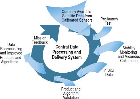Currently Available Satellite Data from Pre-launch Calibrated Sensors Test Mission Feedback Data Central Data Stability Reprocessing Processing and Monitoring and Improved and Vicarious Delivery System Products and Calibration Algorithms In Situ Data Product and Algorithm Validation 3.1.eps FIGURE 3.1 To improve the derivation and ensure the high quality of water-leaving radiance from multiple satellite sensors a single group needs to be responsible for the following: conduct sensor pre-launch tests, ensure that the sensor’s stability is monitored throughout the mis - sion, perform a vicarious calibration, collect in situ data for product and algorithm validation, perform the validation, and routinely process and reprocess the data to improve the products. Once the high-quality water-leaving radiance is produced, users can develop and derive primary and secondary products that satisfy specific requirements of their research or operations. The lessons learned from these steps need to inform and guide current and future missions (adapted from McClain et al., 2002). The ocean color sensor’s design needs to include a plan for both pre-launch and on-orbit performance characterization. Furthermore, sequential reprocessing of ocean color data requires both pre-launch characterization of the system, commitments to conduct on-orbit assessments of instrument performance throughout the mission, and support for the necessary research to improve the models used to derive successful ocean color data products. Hence, the requirements for an ocean color mission are multi-faceted and interconnected. Future plans should reflect this integration of requirements. SOURCE: McClain et al., 2002; NASA’s Goddard Space Flight Center.

OCR for page 28
32 SUSTAINED OCEAN COLOR RESEARCH AND OPERATIONS These and additional requirements for a successful mission satellite sensors ideally would adhere to (Figure 3.2). Beyond are discussed in detail in the following sections. that, one might also request that certain specifications and “metadata” be available for each sensor, so that researchers can evaluate the applicability of each source of satellite data 1. Mission Planning Needs to Include Provisions to to a given study topic. Meet All Requirements, Not Just Sensor Requirements The committee’s guidelines for achieving high-quality A key lesson from CZCS and SeaWiFS is that a suc- sensor performance fall into six general areas: Sensor sta- cessful ocean color mission requires that the team consider bility, waveband selection, scan geometry, sun glint, sensor from the beginning all aspects of what it takes to develop saturation, and polarization sensitivity. Explanations and high-quality ocean color products. For example, CZCS did recommendations are as follows: not have the required in situ monitoring program to ensure high-quality data throughout the entire mission. Because of Sensor Stability the delay in the SeaWiFS launch, additional time was avail- able to build the critical infrastructure, which accounted in The sensor’s stability and monitoring of that stability, is large part for the success of the mission. During the SeaWiFS critical, as demonstrated during the SeaWiFS mission. The and MODIS era, the requirements were strict for the top of monitoring approach depends on the sensor design but needs the atmosphere (TOA) radiometric specifications for the to be an integral part of the overall mission (as discussed satellite mission, and for the algorithms required for quantita- below). SeaWiFS also had a solar diffuser, but that data has tive retrieval of ocean chlorophyll. The TOA specifications not been used for temporal trending of the sensor perfor- were designed to achieve a radiometric accuracy of at least mance because the mission allowed for monthly spacecraft 2 percent absolute (without vicarious calibration) and 1 per- pitch maneuvers to image the moon at a fixed lunar phase cent relative (band-to-band; after vicarious calibration). The angle near full moon. MODIS relies primarily on the solar water-leaving radiances (Lw) in the blue band were to have diffuser data and the diffuser stability monitor. MODIS also an uncertainty of 5 percent or less, with a relative between- views the moon monthly through the deep space port, but band precision of <5 percent and polarization sensitivity of at a higher phase angle (partial moon). VIIRS follows the <2 percent at all angles (Hooker et al., 1992; Hooker and MODIS strategy, but the deep space port is located such that McClain, 2000; McClain et al., 2006; McClain, 2009). the moon is near the horizon and is not visible most of the Experiences with SeaWiFS and other ocean color sen- year without roll maneuvers (Patt et al., 2005). sors show that, by following prescribed steps that begin with R ecommendation: Monitoring of the sensor stability pre-launch sensor characterization and continue throughout should be an integral part of any ocean color mission from the mission, these specifications and other key mission the start. requirements can be met, as is illustrated in Figure 3.1 and in the following sections. Waveband Selection 2. Sensor Design Needs to Consider the Calibration For the CZCS pilot study the 670-nm band had to be and Data Product Requirements When Weighing used for atmospheric correction because the 750-nm band Engineering Trade-Offs was not sensitive enough for the task. Based on the CZCS Sensor designs often attempt to meet the requirements experience, additional bands were added to SeaWiFS (see for a diverse set of applications (see Chapter 2). There- Figure 3.3). SeaWiFS was the first ocean color mission to fore, sensors vary in spatial resolution, specific spectral use NIR bands to enable an atmospheric correction using a band centers, bandwidths, SNR and rated accuracies (see detailed inversion procedure (see below). This approach is Appendix A), as well as data acquisition and timing. These used with MODIS and will be used for VIIRS. variations make it challenging to combine data from differ- MODIS also includes additional bands in the visible that ent sensors to measure trends in ocean biology. Although can be used to quantify chlorophyll a fluorescence. Chloro- there have been efforts to define “standard” ocean color phyll a fluorescence is unique in providing information about sensor characteristics for general applications, establishing physiological states and biological activity. MODIS also common standards may be impractical because sensors for has land remote sensing bands in the Short Wave Infrared different agencies and nations often serve different applica- (SWIR) that can be used in atmospheric correction in turbid tions. However, it is useful to examine lessons from past water conditions (Wang et al., 2009). On MODIS, the 510- sensors and the trade-offs of different design choices with nm band (found on SeaWiFS) was replaced with a band cen- regard to how well one can monitor the sensors’ behavior tered at 532 nm, but this was found to be too highly correlated and stability pre- and post-launch (Table 3.1). Based on our with the 555-nm band to be useful in deriving chlorophyll. examination, the committee is able to provide some simple VIIRS is missing several key wavebands. It has neither guidelines for a minimal set of high-quality standards that all the 510- nor the 532-nm band, which will make it harder to

OCR for page 28
33 LESSONS LEARNED FROM OCEAN COLOR SATELLITE MISSIONS TABLE 3.1 Key Sensor Characteristics CZCSa SeaWiFSb MODISc MERISd VIIRSe Operational Dates Oct. 1978-1986 Sept. 1997-Dec. Terra Dec. 1999- March 2002 - TBD Launch 2012 2010 TBD Aqua March 2002- TBD Ocean Color 4 visible 6 visible 2 NIR 7 visible, 2 NIR, & 9 visible + 6 NIR 5 visible, 2 NIR, & 3 Wavebands 3 SWIR SWIR Scan 45° angle 360° 360° rotating 360° rotating paddle Push-broom imager 360° rotating telescope rotating mirror telescope mirror ±40° scan (1,566 km swath) Sun Glint ±20° fore-aft tilt ±20° fore-aft tilt Terra (1,030) Aqua Nadir view; no sun 1,330 (if available) Avoidance mechanism (2° mechanism (2° (1,330) comparison glint avoidance comparisons increments) increments) Polarization <3 percent, Scrambler ~5 percent <2 percent <2 percent Sensitivity Scrambler SNR 100-150 360-1,000 1,250-2,700 >600-1,400 >1,000 Dynamic Range Ocean only Ocean, land, clouds Ocean only within Ocean color + land Ocean, land, clouds (Sensor Saturation) via bi-linear gain ocean color bands; and clouds via pixel instantaneous control other similar cloud/ automatic gain control land VNIR bands for bright scenes On-board No No 2 solar diffusers Yes Calibration plus an erbium- doped diffuser for spectral calibration Monitoring of No Yes Yes Yes (2 solar Hopefully Stability diffusers) a CZCS: NASA. 2011. Ocean Color Web. [Online]. Available: http://oceancolor.gsfc.nasa.gov/CZCS/czcs_instrument.html [2011, June 7]; Hovis, W.A. et al. 1981. Nimbus 7 coastal ocean color scanner. Applied Optics 20:4175. b SeaWiFS: Barnes, R.A. and A.W. Holmes. 1993. Overview of the SeaWiFS ocean sensor. In Sensor Systems for the Early Earth Observing System Plat - forms, Barnes, W.L. (ed.). Proceedings SPIE 1939:224-232; Barnes, R.A., R.E. Eplee, W.D. Robinson, G.M. Schmidt, F.S. Patt, S.W. Bailey, M. Wang, and C.R. McClain 2000. The calibration of SeaWiFS. In Proceedings of 2000 Conference on Characterization and Radiometric Calibration for Remote Sensing, Logan, Utah, September 19-21, 2000; Barnes, R.A., R.E. Eplee, Jr., G.M. Schmidt, F.S. Patt, and C.R. McClain. 2001. Calibration of SeaWiFS I. direct tech - niques, Applied Optics 40(36):6682-6700; Eplee, R.E., Jr., W.D. Robinson, S.W. Bailey, D.K. Clark, P.J. Werdell, M. Wang, R.A. Barnes, and C.R. McClain. 2001. Calibration of SeaWiFS. II. Vicarious Techniques. Applied Optics 40(36):6701-6718; Hammann, M.G. and J.J. Puschell. SeaWiFS-2: An ocean color data continuity mission to address climate change. In Remote Sensing System Engineering II, Ardanuy, P.E., and J.J. Puschell (eds.). Proceedings of SPIE 7458:745804. c MODIS: Guenther, B., W. Barnes, E. Knight, J. Barker, J. Harnden, R. Weber, M. Roberto, G. Godden, H. Montgomery, and P. Abel. 1995. MODIS Calibration: A brief review of the strategy for the at-launch calibration approach. Journal of Atmospheric and Oceanic Technology 13:274-285; Schueler, C.F. and W.L. Barnes. 1998. Next-generation MODIS for polar operational environmental satellites. Journal of Atmospheric and Oceanic Technology 15:430-439. d MERIS: Curran, P.J. and C.M. Steele. 2005. MERIS: The re-branding of an ocean sensor. International Journal of Remote Sensing 26:1781-1798. e VIIRS: Schueler, C.F., P. Ardanuy, P. Kealy, S. Miller, F. DeLuccia, M. Haas, H. Swenson, and S. Cota. 2002. Remote sensing system optimization. Aerospace Proceedings 4:1635-1647; Schueler, C.F., J.E. Clement, P. Ardanuy, M.C. Welsch, F. DeLuccia, and H. Swenson. 2002. NPOESS VIIRS sensor design overview. In Earth Observing Systems VI, Barnes, W.L. (ed.). Proceedings of SPIE 4483:11-23. retrieve chlorophyll concentrations in optically turbid waters. (10 nm) band is needed near the fluorescence peak (MODIS It is also missing the chlorophyll fluorescence bands and sen- uses 678 nm to avoid atmospheric absorption features) and sitive SWIR bands. It is critical to have the appropriate bands bands on either side of the fluorescence peak (MODIS uses for the atmospheric correction. SeaWiFS NIR SNRs were 667 and 748 nm). too low, whereas those of MODIS and VIIRS are acceptable. One major issue plaguing ocean color imagers is the sep- SWIR bands are useful in turbid waters; both MODIS and aration of algal and non-algal absorption coefficients from VIIRS SWIR bands have low SNRs (higher SNR is recom- ocean color signals, especially as the climate changes. Exist- mended). To retrieve chlorophyll a fluorescence line height ing methods (Lee et al., 2002; Siegel et al., 2002, 2005a,b; (Letelier and Abbott, 1996; Behrenfeld et al., 2009), a narrow Morel, 2009; Morel and Gentili, 2009) all leverage their

OCR for page 28
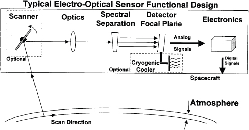
34 SUSTAINED OCEAN COLOR RESEARCH AND OPERATIONS FIGURE 3.2 Ocean color sensor functional elements. This figure uses the example of a scanner to illustrate the fundamental sensor design 3.2.eps elements comprising an EOS sensor for ocean color (or other) applications. SOURCE: Acker et al., 2002a. bitmap are much stronger than ocean color signals.2 With this new success from differentiating the colored dissolved organic matter (CDOM) absorption signal from the algal absorption information, future atmospheric correction/ocean color based on information from a single channel, 412 nm (Lee et algorithms likely will be coupled inversions similar to those al., 2002; Maritorena et al., 2002; Morel and Gentili, 2009). trailblazed by Professor Howard Gordon and his students The present operational algorithm for SeaWiFS and MODIS (e.g., Chomko and Gordon, 2001; Chomko et al., 2003). uses four wavelengths to derive chlorophyll concentrations. To ensure continuity of Type 1 ocean color observa- A single band for discriminating non-algal absorption, such tions, a minimum band-set needs to be maintained on future as CDOM, limits the assessment of portioning uncertainty sensors. The ideal Type 1 sensor would have at minimum (there is only one degree of freedom). CDOM absorption, the following bands in the visible: 412, 443, 490, 510, 555, the major constituent that needs to be portioned from phyto- 667, 678, and 765 nm, which is a combination of the bands plankton absorption, increases with shorter wavelengths, and present on SeaWiFS and MODIS (SeaWiFS = 412, 443, CDOM dominates the absorption spectrum in the near-ultra- 490, 510, 555, 675 nm; MODIS = 412, 443, 490, 531, 555, violet (UV; Nelson and Siegel, 2002; Nelson et al., 2010). 667, 678, and 748 nm). As described above, two channels in Present plans for PACE and Aerosol-Cloud-Ecosystems the near-UV would be useful for partitioning algal and non- (ACE) include wavebands in the near-UV (350, 360, and 385 algal absorption optical properties and for implementing new nm) to better enable this partitioning.1 Inclusion of several algorithms for absorbing aerosols. The ACE science team bands in the near-UV would help in separation of algal and recommends bands centered on 360 and 385 nm for these non-algal ocean color signals. purposes; the committee supports this finding. In addition, Bands in the near-UV likely will be important for the sensor would require some SWIR and NIR bands in the improving atmospheric correction procedures. Absorbing atmospheric “windows.” aerosols have long confounded existing atmospheric correc- Recommendation: Spectral band-sets for sustaining exist- tion methods, as these methods require that aerosol contri- ing ocean color capabilities should be at least as complete butions in the visible spectrum can be modeled by knowing as the SeaWiFS band-set, preferably with improved SNR NIR aerosol radiance characteristics (Gordon and Wang, values, SWIR bands with improved SNR values for atmo- 1994a; Gordon, 1997). The presence of absorbing aerosols, spheric corrections in turbid waters, the ability to retrieve generally from land sources (pollution, dust, etc.), makes chlorophyll a fluorescence, and near-UV bands for improv- atmospheric correction models fail under such conditions ing the partitioning of algal and non-algal ocean color sig- (Gordon, 1997; Gordon et al., 1997; Moulin et al., 2001). nals and for implementing new approaches in atmospheric The near-UV provides a path for correcting for absorbing correction. aerosols because the atmospheric signals in the near-UV 1 2 ACE 2010 White Paper. Available at: http://www.neptune.gsfc.nasa. ACE 2010 White Paper. Available at: http://www.neptune.gsfc.nasa. gov/.../ACE_ocean_white_paper_appendix_5Mar10.doc. gov/.../ACE_ocean_white_paper_appendix_5Mar10.doc.

OCR for page 28
35 LESSONS LEARNED FROM OCEAN COLOR SATELLITE MISSIONS HERITAGE SENSORS “Multispectral” ocean bands MODIS on Aqua (1997–2010 ) (1978–1985) CZCS: 4 SeaWiFS (2002– )* SeaWiFS: 8 CZCS MODIS: 9 VIIRS VIIRS: 7 Ultraviolet Products No Measurements Total pigment or chlorophyll-a but major errors due to absorption by dissolved organics Visible Atmospheric correction/ MODIS chlorophyll fluorescence Atmospheric correction NIR (clear ocean) Atmospheric correction SWIR (coastal) ** * MODIS on Terra was launched in 2000, but does not yet provide science-quality ocean color data. * * MODIS/Visible Infrared Imaging Radiometer Suite (VIIRS) SWIR bands are not optimized for oceans. 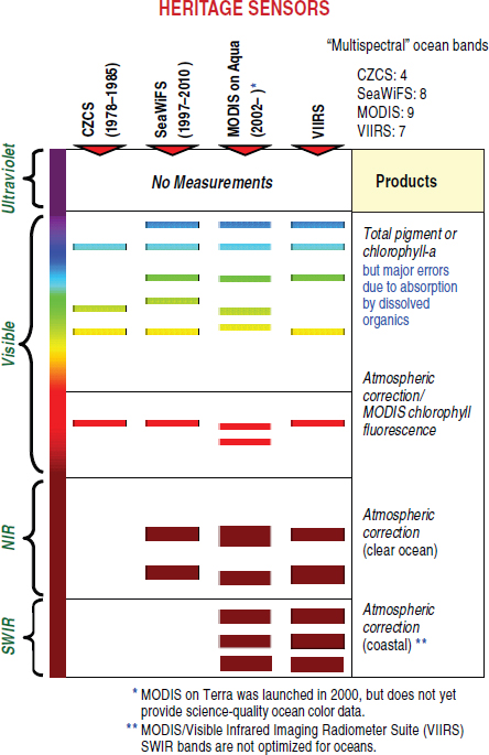FIGURE 3.3 Comparison of spectral coverage of heritage sensors. 3.3.eps SOURCE: Adapted with permission from Charles McClain, NASA/Goddard Space Flight Center. Scan Geometry read out simultaneously at the same scan mirror position at any Earth location. Different spectral bands on the same Sensor scan geometry impacts the reprocessing of ocean MODIS focal plane (e.g., ocean color bands) are read out at color data. SeaWiFS and MODIS reprocessing differ based different times so that the scan mirror is at a different angle on their different scan geometry. SeaWiFS used a rotating for each band at any Earth location. This affects reflectance telescope to provide a cross-track scan, and detectors in one and vicarious calibration differently than for SeaWiFS, and spectral band see different geometry because they are aligned complicates the calibration procedures for MODIS compared along-scan and read out sequentially as the telescope rotates. with SeaWiFS. Different spectral bands are displaced along-track (cross-scan), however, so that all bands are read out with the Conclusion: When designing a new sensor, it is important same scan geometry at any Earth location. MODIS uses a to consider how the sensor’s design may impact the vicari- cross-track scan mirror. The MODIS detectors in a spectral ous calibration and periodic data reprocessing. band are aligned cross-scan (along-track) so that they are

OCR for page 28
36 SUSTAINED OCEAN COLOR RESEARCH AND OPERATIONS Sun Glint quately for eliminating saturation over all targets, whereas MODIS employs two independent channels in each such Sun glint comes from the reflection of sunlight from band, one at high gain with lower dynamic range for ocean the ocean’s surface into the viewing path of the sensor. color, and the other with low gain and high dynamic range. Retrievals of Lw are nearly impossible for those illumina- VIIRS uses a single dual-gain channel for each band with tion and viewing angles contaminated by sun glint (Gordon automatic gain control. and Wang, 1994b). Existing ocean color algorithms exclude pixels found within the sun-glint pattern (Wang and Bailey, Recommendation: The ocean color sensor design should 2001). Sensor and mission design can help mitigate these ensure that saturation can be avoided under any environ- issues. The CZCS and SeaWiFS sensors were both tilted mental conditions, yet resolve ocean color signals for the away from the sun’s specular path by 20 degrees to avoid effective retrieval of water-leaving radiance spectra. sun glint. MODIS (and VIIRS) is nadir-looking (i.e., with- out a tilt looking straight down) (Table 4.1). Thus, sun glint contaminates much of MODIS’s viewing geometry under Polarization Sensitivity high zenith angle conditions such as found in the tropics near Minimal polarization sensitivity is required. Many of noon. This limits the effective spatial coverage by MODIS the problems with the processing of MODIS-Terra imagery in the tropical oceans (Gregg et al., 2005; Maritorena et al., are related to the time-dependent polarization sensitivity 2010). The plans for avoiding sun glint for the two MODIS (Franz et al., 2008; Kwiatkowska et al., 2008). Some refine- missions were to use observations from different equatorial ments of the MODIS-Aqua characterization using the same crossing times. This approach is problematic as it assumes technique were needed in the most recent reprocessing, but that MODIS on Terra and Aqua produce similar data streams the corrections were much smaller than for MODIS Terra. and that a vicarious calibration for both can still be achieved. However, use of a polarization descrambler precludes the simultaneous viewing of thermal infrared bands, as is done Recommendation: Future ocean color sensors should now in MODIS and VIIRS. Most recently, requirements for avoid sun glint by tilting the sensors’ viewing away from polarization sensitivity are <1 percent. sun-glint contaminated regions of the oceans. Recommendation: Future ocean color sensors should min- Sensor Saturation imize the polarization sensitivity and residual polarization should be adequately characterized in pre-launch testing. Avoiding sensor saturation presents a challenge because the signal from clouds and the atmosphere is very high com- 3. The Sensor Has to Be Well Characterized Prior to pared with the signal from the ocean. Because most (>90 Launch percent) of the signal detected by the satellite stems from light scattered in the atmosphere, successful ocean color The SeaWiFS and MODIS missions demonstrated the remote sensing depends on correcting for the radiance from importance of pre-launch sensor characterization because the atmosphere. Therefore, measurements of atmospheric many factors needed for data processing cannot be easily signals in both ocean color and aerosol bands are required. characterized in orbit (McClain et al., 2006). These factors Avoiding saturation while also providing sufficient signal include temperature effects, stray light, optical and electronic sensitivity in the ocean color bands requires either dual cross-talk, band-to-band spatial registration, relative spectral simultaneous measurements in each band, or dual-gain, and out-of-band response, signal-to-noise ratios, electronic preferably with instantaneous automatic gain control. Dual- gain ratios, polarization sensitivity, response versus scan gain band offset and gain coefficients differ for each gain. angle, and any instrument specific items, such as selec- The coefficients are downlinked with the raw data and a flag tive detector aggregation, that can impact sensor response indicating the gain the detector was in when the measurement (McClain et al., 2006). Because it is often impossible to de- was made. Then the offset and gain coefficients are applied to convolve sources of error post-launch, these attributes need achieve <2 percent radiometric error. Short-term (in the order to be determined prior to launch. of a second) detector response instability may cause a small These characteristics vary greatly from sensor to sensor. intra-scan, temporally varying, offset and gain coefficient For example, MODIS, unlike SeaWiFS, has multiple detec- error (affects single- and dual-gain bands). Vicarious cali- tors per spectral band and the radiometric and polarization bration is, as shown in Appendix B, insensitive to offset and sensitivity is specific to each detector. Measurements of gain error and therefore insensitive to instability. Therefore, MODIS’s polarization sensitivity were questionable and vicarious calibration is applied for ocean color applications led to a seasonal latitude- and time-dependent error in the to achieve overall levels of radiometric uncertainties of 0.3 retrieved water-leaving radiances (NASA, 2009a). An impor- percent or less. tant part of the characterization process is to allow for free SeaWiFS used a bi-linear gain feature that worked ade- and open discussions between the vendor, representatives of

OCR for page 28
37 LESSONS LEARNED FROM OCEAN COLOR SATELLITE MISSIONS 4. Vicarious Calibration Is Required to Achieve the sponsoring agency and experts from the user community. On-Orbit Accuracy Goals For both MODIS and SeaWiFS, productive interchanges between vendor, agency, and user community resolved Although satellite sensors are calibrated prior to launch, problems prior to launch, and also post-launch as part of their calibration coefficients likely change during the storage reprocessing efforts. These discussions also effectively lev- period prior to launch, during the launch, and in orbit while eraged the vendor personnel’s knowledge of the sensor with exposed to the hostile space environment. This potential for the agency personnel’s knowledge of algorithm development change requires a post-launch assessment and adjustment and cal/val needs. of the pre-launch calibration coefficients. The standard and Because VIIRS was procured as a performance-based most reliable procedure to achieve such an assessment is a contract, it minimized such interactions between vendor vicarious calibration (Franz et al., 2007; McClain, 2009; and agency personnel. Many initial issues with the VIIRS see also Appendix B). Vicarious calibration is a process sensor set to launch on National Polar-orbiting Operational to calibrate a satellite ocean color sensor after launch that Environmental Satellite System Preparatory Project (NPP) begins with high-quality in situ measurements of Lw at the were due to pre-launch characterization results that did same wavelength band (preferably also accounting for the not meet specifications. Subsequent testing and end-to- out-of-band response) as for the satellite sensor. Because end system testing performed after VIIRS was mated with the Lw signal reaching a satellite ocean color sensor is the NPP spacecraft have shown much better performance small compared to the contribution of backscattered atmo- characteristics for VIIRS. Some of these discrepancies spheric radiances, vicarious calibration of satellite ocean were due to differences in the test facilities used to test and color sensors also requires that the Lw signal be accurately characterize VIIRS (Turpie, 2010). This demonstrates that propagated via models and calculations from the ocean test facilities themselves must be adequately designed and surface, through the atmosphere and to the satellite sensor. tested for the pre-launch characterization of ocean color Accurately propagating the Lw signal to satellite altitudes is sensors. Further, International Traffic in Arms Regulations easier and more accurate at locations where the contribu- (ITAR)3 restrictions have prohibited open access to the test tion of the most variable optically active components of program dataset for VIIRS. Such restrictions could seriously the atmosphere (e.g., aerosols) are small, or at worst, suf- compromise the ability of the U.S. community to acquire ficiently well-characterized. Thus, the location of vicarious similar information for foreign sensors. Similar concerns calibration sites is critical. Experience with SeaWiFS and exist about “trade secrets” that would prohibit instrument MODIS shows that many observations (at least 50; see also vendors from openly sharing instrument design information Appendix B) are required before stable and accurate values with all affected parties. can be determined for adjusting the calibration coefficients Because any ocean color sensor will need repeated of the satellite sensor (Franz et al., 2007). Because of sun- vicarious calibrations, the pre-launch absolute radiometric glint contamination, nadir-viewing ocean color missions will calibration is not as critical, and pre-launch absolute radio- take much longer than tilting sensors to achieve a sufficient metric calibration uncertainties of ~5 percent may be accept- number of calibration match-ups. able. This relaxing of requirements would help constrain Given the strict accuracy requirements, field instru- instrument costs. ments used for vicarious calibration have to measure Lw with accuracy on the order of a few percent to implement Recommendation: An aggressive pre-launch characteriza- quantitative algorithms (e.g., McClain et al., 2004). This tion program should be in place for those factors that are accuracy is extremely difficult to achieve and requires high- not easily adjusted on-orbit with validated test facilities. quality in situ instrumentation, accurate models to correct for atmospheric path radiance, and a rigorous process for Recommendation: Open communication and frequent both acquiring the in situ measurements and for matching interactions among the sensor vendor, agency personnel, the in situ and satellite measurements. This requirement for and the relevant instrument team should be pursued to field observations was achieved for SeaWiFS and MODIS efficiently leverage knowledge and quickly identify design using MOBY (Clark et al., 2002; see Appendix B). MOBY and algorithm solutions. has been extensively characterized using National Institute of Standards and Technology (NIST) resources and is well suited to understand the in-band, out-of-band, and cross-talk responses of the MOBY instrument, permitting proper de- convolution of these signals to obtain the true water-leaving 3 The International Traffic in Arms Regulations (ITAR) pertain to export and import of ITAR-controlled defense articles, services, and technologies. radiance spectrum (Carol Johnson, personal communica- It also protects export/import of technology pertaining to satellites and tion; see Appendix B). A dedicated team for developing and launch vehicles. As a result, some information exchange related to sensor maintaining these standard measurements is critical, given pre-launch and post-launch calibrations could be restricted by ITAR (NRC the need to maintain strict accuracy over the duration of the 2008c: Space Science and the International Traffic in Arms Regulations: Summary of a Workshop).

OCR for page 28
38 SUSTAINED OCEAN COLOR RESEARCH AND OPERATIONS satellite mission and beyond (to use these measurements for observations at the same phase angle. In general, it cannot be satellite data inter-calibration). assumed that the degradation is straightforward to model or The approach with MOBY was to develop and imple- that frequent match-ups are available due to sun-glint issues. ment a robust, rigorous facility to support continuous in situ For nadir-viewing ocean color missions such as MODIS and measurements of water-leaving, spectrally continuous (i.e., VIIRS, the calibration will take much longer because of sun- hyperspectral) radiances. From hyperspectral measurements, glint contamination. The contributions of uncertainties in the MOBY water-leaving radiance (Lw(λ)) determinations to the one can synthesize the band-set of any satellite ocean color sensor. The buoy approach was based on the lessons learned vicarious calibration involve both the MOBY spectrometer from the CZCS mission, during which measurements for calibration and the propagation of the subsurface radiances the vicarious calibration were performed from ships during through the water column and the air-sea interface. Brown the early phase of the mission. MOBY operates 365 days et al. (2007; Table 5) showed that the total uncertainty in MOBY determinations of Lw(λ) under excellent conditions a year, taking measurements three times a day, timed with the overpasses for SeaWiFS and MODIS-Aqua and -Terra. ranged from 2.1 to 3.3 percent depending on the spectral band. The Lw(λ) contribution to the top of the atmosphere From July 1997 to February 2007, 8,347 measurements were made. However, it is not possible to have a satellite match-up radiance is typically 10 percent for oligotrophic waters and for every MOBY observation (Franz et al., 2007). Clouds clear atmospheres, which are typically found where MOBY has been deployed. Thus, the Lw(λ) uncertainty to TOA radi- obscure satellite views of the ocean. In general, clouds build up during the afternoon, which means the satellite ance is equivalent to 0.21 to 0.33 percent at the top of the orbital parameters influence the number of useful match- atmosphere, the major source of uncertainty to the SeaWiFS ups. Clouds are one rejection criteria for match-ups between overall uncertainty budget. MOBY and satellite sensors; other limiting factors include Based on lessons learned from SeaWiFS, MODIS, and instrument problems. Of the 8,347 measurements collected other sensors, vicarious calibration has to meet certain cri- during the one-year interval ending in February 2007, about teria. The site needs to be in oligotrophic waters but acces- 45 percent of the data were cloud contaminated. About 10 sible without excessive ship costs. Islands are the logical percent were flagged as questionable, and 45 percent were choice but clouds form around islands—for example, on the good. During the beginning of the SeaWiFS mission, every windward side of Hawaii, with its high mountain ranges. The possible match-up was utilized (Eplee et al., 2001). As the leeward side is a better option. The site requires extensive research of the SeaWiFS calibration continued, the selec- characterization, including optical, biophysical, and biogeo- tion criteria were improved and a reduction in the number chemical, and this requires experienced researchers and ship of match-ups was justified, but it took almost four years time to measure, for example, the bi-directional reflectance to get the 30 match-ups that meet the current criteria. The distribution function. The ideal site would provide a nearby Ocean Biology Processing Group (OBPG) at NASA’s God- facility for maintenance and related functions including: dard Space Flight Center (GSFC) excludes data if: 1) the refurbishment, in-field servicing, improvement of the hard- two measures of the water-leaving radiance that are derived ware of the optical buoy and the mooring buoy, radiometric from the three different depths using MOBY disagree by characterization, and pre- and post-deployment calibration more than 5 percent; or 2) the measured surface irradiance for the in situ instrument. In addition, data analysis and data differs from a clear-sky irradiance model by more than 10 archiving are critical aspects of the vicarious calibration percent. Satellite sensor datasets are excluded if: (1) there facility operations. are any flagged (suspicious) pixels in the image; (2) the Conclusion: The importance of a vicarious calibration mean chlorophyll-a concentration retrieved for the scene is cannot be overstated. Based on empirical studies conducted greater than 0.2 mg/m3, which is unusually high for such over the past 15 years with ocean color as well as atmo- oligotrophic waters found at the MOBY site; (3) the retrieved spheric and land data, NIST has determined that vicarious aerosol optical thickness in the near-infrared is greater than calibration, using surface-truth measurements to compare 0.15 (note this could be an indicator of sun-glint contamina- with satellite measurements, is necessary to calibrate the tion, not actual aerosol contribution); (4) the satellite view sensor after the launch, including setting/re-setting the angle is greater than 56 degrees; or (5) the solar zenith angle instrument gain factors. is greater than 70 degrees (Franz et al., 2007). These criteria resulted in only 15 match-ups per year over nine years of Conclusion: MOBY or a MOBY-like effort is necessary MOBY/SeaWiFS continuous operations (Franz et al., 2007). for the continuation of ocean color climate data records. Franz et al. (2007) conclude that it would take two to Although other approaches might produce acceptable three years of continuous in situ operations in order to estab- vicarious calibration data, they have not been widely lish the calibration of an ocean color sensor with character- implemented or deployed operationally. MOBY is currently istics similar to SeaWiFS. However, it should be pointed out the accepted standard for a vicarious calibration source that the nature of the SeaWiFS degradation was straightfor- and is already deployed. Further, non-U.S. sensors (such ward to model and to predict, and there were frequent lunar

OCR for page 28
39 LESSONS LEARNED FROM OCEAN COLOR SATELLITE MISSIONS as MERIS) use MOBY as a vicarious calibration source, that have multi-detector imagers, because lunar views image which will make it easier to link U.S. and international only a small portion of the observed area and include only datasets. a few detectors. The advantage of using the moon directly as a stability source is that the relatively weak and diffuse Conclusion: To maintain SeaWiFS accuracies in retriev- sunlight radiance reflected from the moon can be viewed ing water-leaving radiance, a sensor’s overall uncertainty directly through the same optics as the ocean, i.e., without level for calibration gains needs to be constrained below 0.3 using a diffuser or separate optical path to the satellite sen - percent (see Appendix B). This can only be accomplished sor. This minimizes concerns that diffuser characteristics can by a vicarious calibration, which needs to begin at the start change during the satellite mission. In addition, observing of the mission to achieve this accuracy. the moon has the advantage of providing sensor observations acquired at radiance levels more nearly equivalent to top of the atmospheric Earth-viewed radiance. 5. Stability Monitoring: Lunar Calibration or Another For both SeaWiFS and MODIS-Aqua, individual spec- Proven Mechanism for Stability Monitoring Is tral channels degraded at different rates with time (Figure Required to Achieve Radiometric Stability Goals 3.4). Over the first nine years of SeaWiFS observations, the 865-nm band degraded the most (18 percent). In contrast, for In addition to vicarious calibration, temporal changes MODIS-Aqua, a sensitivity loss of 15 percent at 412 nm dur- in sensor radiometric calibration need to be determined ing a four-year period was the most for any of Aqua’s ocean throughout the mission, and corrections need to be made for color bands (McClain et al., 2006). The relatively rapid and observed rate of degradation, to ensure high-quality ocean significant degradation of the SeaWiFS 865-nm band relative color data (e.g., Eplee et al., 2004; McClain, 2009). The to the other spectral bands would have made accurate atmo- experience with SeaWiFS shows that different spectral chan- spheric correction difficult if not impossible to implement nels degrade at different rates (Figure 3.4) and independent without applying the degradation corrections. It is equally corrections must be applied to each spectral band. important that the degradation be determined throughout Because of the success of the SeaWiFS lunar imaging- the mission. An example is that while the SeaWiFS 865-nm based stability monitoring, this methodology has been band followed a well-characterized pattern during the first incorporated into the MODIS on-orbit performance analyses nine years of on-orbit operations, it subsequently changed its and adopted by other missions prior to launch, e.g., Ocean decay trend. Without ongoing measurements of sensor deg- Colour Monitor on-board Oceansat-2 (OCM-2). It should radation, this important change in behavior would not have be noted that this is a relative measurement, not an absolute been detected, leading to deterioration of product accuracy. calibration. MERIS employs an alternative approach using Importantly, the deviations in the SeaWiFS lunar cali- two solar diffusers: one with frequent solar observations bration observations from the fit equations used to correct for to monitor the sensor stability, and a second diffuser with sensor drift are very small, here less than 0.1 percent. Note infrequent solar observations to monitor the degradation of that the level of uncertainty in the stability characterization the first. Multiple concurrent solar diffusers are important for is less than the uncertainty in the vicarious calibration (see assessing impacts of stability if the moon is not used as the Appendix B) and points to the excellent qualities of the moon standard. In addition to lunar views, solar diffusers may be as a stability source for ocean color sensor characterization. 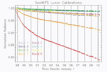required for stability monitoring of sensors such as MERIS FIGURE 3.4 SeaWiFS lunar calibrations (Patt, personal commu- nication, 2010). Deviations from the fitting functions are less than 0.1 percent for all bands. SOURCE: Ocean Color Biology Group, NASA’s Goddard Space Flight Center. 3.4.eps bitmap

OCR for page 28
40 SUSTAINED OCEAN COLOR RESEARCH AND OPERATIONS Conclusion: Stability monitoring is of highest priority. Recommendation: New satellite missions need to demon- Monitoring instrument stability can constrain the sensor strate that their Lw measurements are consistent with those changes within 0.1 percent by viewing an appropriate obtained by prior missions, particularly prior missions for source (such as the moon). which considerable validation and vicarious calibration data were obtained. This is an essential requirement for Recommendation: Future ocean color sensors should view developing sustained ocean color time-series for scientific the moon at least monthly through the Earth-view port to analyses. monitor the sensor’s stability throughout its mission. 7. End-to-End Validation of Ocean Color Products Is 6. Mission Overlap Is Essential to Transfer Critical and a Key Step in the Reprocessing of Ocean Calibrations between Sensors (e.g., SeaWiFS was used Color Data Products to help transfer calibrations to MODIS) Validation programs4 are required to ensure that the Mission overlap was essential for enabling high-quality algorithms that generate data products from satellite radi- ocean color data from both the MODIS-Aqua and MODIS- ances are credible with data users and that the models and Terra sensors. The calibration for MODIS, an instrument that procedures used to process the datasets are working appro- shares a number of challenging design features with VIIRS, priately. Validation is also a key step in the reprocessing of is complicated. It was fortunate that observations from Sea- ocean color data products (Figure 3.1). Algorithm devel - WiFS were available, with its well-studied calibration and opment is an active area of research conducted by many product validation history and a sensor based on a simple independent research labs. To take advantage of community design (e.g., constant angle of incidence scan system vs. findings, an effort is required to compare and validate various MODIS variable angle incidence scan). Water-leaving radi- algorithms and products. Validation programs for SeaWiFS ances derived from SeaWiFS observations were employed as and MODIS included comparisons of satellite with in situ Lw, reference radiances to study the seasonal, latitudinal, cross- i.e., comparisons of derived ocean color data products such scan, and polarization behavior of the water-leaving radi- as chlorophyll, particulate organic carbon (POC), particulate ances for MODIS on Aqua and Terra (Kwiatkowska et al., inorganic carbon (PIC), and CDOM with in situ data, and 2008; NASA, 2009b). These comparisons served to validate comparisons of aerosol characteristics used to correct for the the various corrections used to determine the actual MODIS- atmospheric path radiance with field observations. Validation Aqua polarization response. Eventually, MODIS-Aqua and requires match-up datasets that can be used to compare sat- SeaWiFS Lw converged. However, without access to well- ellite data performance with field observations (Bailey and characterized SeaWiFS products that had been validated Werdell, 2006). Given the high costs of ship time and other against extensive in situ observations, accurate MODIS- fixed costs, ideal validation programs produce comprehen- Aqua Lw would not have been achieved. This underscores sive ocean-atmosphere datasets to meet multiple purposes. the justification for extensive pre-launch characterization. Appendix C describes the measurements needed for com- Mission overlap also was required to assess the high prehensive datasets. Validation of aerosol data products is as quality of the MODIS-Terra dataset, which was complicated essential as validation of in-water properties. For SeaWiFS by time-dependent changes in the gains and polarization and MODIS, aerosol validation was provided by measure- sensitivity as a function of scan angle (Kwiatkowska et al., ments from a network of sun photometers (Knobelspiesse 2008). Given these sources of uncertainty, the retrieval of et al., 2004). The results of these comparisons are then used climate-quality water-leaving radiance observations from the to assess how to improve the data products through itera- MODIS-Terra mission was possible only after comparison tive changes to sensor calibration and/or retrieval models with near simultaneous data from SeaWiFS and MODIS- (Figure 3.1). Aqua. To best account for these sources of uncertainty, a To facilitate the algorithm development and data prod- vicarious calibration procedure was employed for MODIS- uct validations for SeaWiFS, the Goddard Ocean Color Terra, using SeaWiFS as truth, to simultaneously correct Data Reprocessing Group maintains a repository of in situ for the time-dependent changes in gains and polarization marine bio-optical data, the SeaWiFS Bio-optical Archive sensitivity (Kwiatkowska et al., 2008; Franz et al., 2008). and Storage System (SeaBASS; seabass.gsfc.nasa.gov). The T his demonstrates the utility of simultaneous satellite acquisition and analysis of the in situ measurements has been observations to best characterize on-orbit changes in instru- an international collaboration (e.g., the Atlantic Meridional ment responses. This methodology of comparing multiple Transect program), which greatly enhances the global distri- satellites also has been used in the on-orbit assessments of bution of data in SeaBASS. Acquisition of these observations MODIS-Aqua responses (NASA, 2009b). We must also note 4 “Validation is the process of determining the spatial and temporal error the unfortunate fact that the VIIRS mission will not overlap fields of a given biological or geophysical data product and includes the with SeaWiFS. development of comparison or match-up data set.” From http://www.ioccg. org/reports/simbios/simbios.html.

OCR for page 28
41 LESSONS LEARNED FROM OCEAN COLOR SATELLITE MISSIONS is time consuming and resource intensive; sharing of data and result of reprocessing. For example, the initial processing of resources across the community is vital to obtain adequate SeaWiFS imagery yielded negative values for water-leaving coverage in space and time. These data were used to compile radiance for continental shelf waters in the band centered at a large set of pigment concentrations, biogeochemical vari- 412 nm and depressed values at 443 nm. This difficult prob- ables, and inherent optical properties. This new dataset, the lem was not fully resolved until the data were reprocessed NASA bio-Optical Marine Algorithm Dataset (NOMAD), many times (e.g., Patt et al., 2003; McClain, 2009). In 2009, includes more than 3,400 stations of Lw, surface irradiances, the reprocessing of the MODIS-Aqua dataset corrected and diffuse downwelling attenuation coefficients. Metadata, another, much more subtle drift in the 412-nm water-leaving such as the date, time, and location of data collection, and radiance, which had resulted in an apparent dramatic increase ancillary data, including sea surface temperatures and water in CDOM concentration in the open ocean (Maritorena et depths, accompany each record (Werdell and Bailey, 2005). al., 2010). Global data coverage is needed to create global bio-optical Reprocessing requires appropriate computational tools algorithms, to test their performance in particular regions, so that the entire dataset can be processed rapidly, enabling and to develop regionally specific algorithms. changes between algorithm or calibration selections to be quickly evaluated. This ability to rapidly reprocess the Conclusion: To derive and validate the desired ocean entire data stream was planned for the SeaWiFS mission. color data products from water-leaving radiance, in situ Fortunately, the price to performance ratio for commodity data representing the range of global ocean conditions is computer hardware has decreased dramatically since the needed for algorithm development and product validation. launch of SeaWiFS, which makes it much easier to configure These in situ data need to be collected, properly archived and run reprocessing experiments with multiple datasets. and documented, and widely available through a database Reprocessing of ocean color datasets also is critical for such as SeaBASS. The global requirements of this database developing decadal-scale records across multiple missions. suggest that these data are to be shared among all interna- Antoine et al. (2005) developed a decadal-scale ocean color tional participants. data record by linking the CZCS data record to the SeaWiFS era. Key to their approach was the reprocessing of both Conclusion: All ocean color missions require product vali- datasets using similar algorithms and sources. The result- dation programs as a key step in the reprocessing of ocean ing decadal ocean color time-series shows many interesting color observations and to establish uncertainty levels for climate patterns supporting their approach (Martinez et al., ocean color mission data products. 2009). Thus it is likely that the best approach to creating multi-decadal ocean color data products is the simultaneous reprocessing of multiple ocean color missions with similar 8. Satellite Ocean Color Products Need Continual algorithms and the same vicarious calibration sources, if Reprocessing to Assess Climate-Scale Changes in the possible (Siegel and Franz, 2010). Ocean Biosphere, and Reprocessing Is an Important Element in Developing Multi-Decadal Ocean Color Conclusion: Reprocessing is important and needs to be Datasets incorporated into the mission plan and budget process from the beginning, with provisions for the computational ability The importance of reprocessing mission data at regular to rapidly reprocess the entire dataset as it increases in size. intervals throughout the mission became apparent dur- ing both SeaWiFS and MODIS missions (McClain, 2009; Conclusion: Reprocessing of multiple missions referenced Siegel and Franz, 2010). Much is learned during the mission to the same vicarious calibration sources is likely the only about the sensor’s behavior and the atmospheric correction, way to construct long-term ocean color data products. bio-optical, and data high-quality mask/flag algorithms for converting Lw into ocean color products. Data reprocessing is needed to adjust for the following changes: (1) to the calibra- 9. The External U.S. and International Science tion coefficients due to sensor degradation, (2) to in-water Community Needs to Be Routinely Included in and atmospheric correction algorithms based on validation Evaluating Sensor Performance, Product Validation, results, and (3) in availability of new algorithms for new and and Other Updates to Ocean Color Data Products improved data products. In addition, as discussed above, it takes many match-ups before the vicarious calibration can One of the unique strengths of the SeaWiFS mission achieve the desired accuracy and stability for the sensor’s was how well it engaged the U.S. and international science gain factor. Therefore, data processing and product genera- community of ocean color data users, as well as those with tion cannot be expected to produce high-quality products at technical knowledge and insight on satellite data processing the beginning of a new mission. and bio-optical measurements. Although all NASA science For all these reasons, data product quality will improve missions have science teams, the Ocean Biology and Bio- as more is learned about the sensor’s behavior and as a geochemistry program is unique in hosting annual Ocean

OCR for page 28
42 SUSTAINED OCEAN COLOR RESEARCH AND OPERATIONS Color Research Team meetings that are open to anyone. tional exchange of raw satellite data and detailed calibra- In this way, the SeaWiFS Project received input from a tion information. Such restrictions could seriously impede broad international group of scientists on algorithms, data international cooperation, making it even more challenging quality, data products, validation, and other topics, from to produce long time-series of ocean color products that are pre-launch throughout the mission. As a result, the project essential for determining if the ocean biology is changing in received important and unanticipated contributions that led response to a changing climate. to significant improvements. For example, the at-launch ITAR restrictions may present the biggest problems chlorophyll algorithm for SeaWiFS (OC-4) emerged from a when users attempt to exchange information about the sen- community-led meeting that compared a wide suite of model sor characteristics. Algorithms and reprocessing details are formulations (O’Reilly et al., 1998). Another important generally well documented for NASA ocean color satellite advantage of open engagement is that the international user missions, including SeaWiFS and MODIS. The SeaWiFS community develops a sense of ownership of the mission, project also documented many important technical and which leads to considerable international cooperation. For other aspects of the mission, producing 43 pre-launch and example, members of the SeaWiFS project involved with 29 post-launch technical reports on topics such as optics algorithms and validation were invited as participants in the protocols, description of the bio-optical archive, results of United Kingdom-supported Atlantic Meridional Transect inter-calibration exercises for in situ measurements, and orbit cruises (Aiken et al., 2000), which provided a key source of analysis. These documents are extremely valuable to users in situ data across many bio-optical regimes. and to those planning future missions, including international partners. For the recent satellite ocean color reprocessing Conclusion: Annual ocean color technical meetings among effort, these printed documents appear first as Web-based U.S. and international researchers and space agency reports5 that show the effects of virtually every change on personnel will create many opportunities for cooperative the final data products. calibration and validation programs, improvements to algorithms, and coordination of ocean color mission data Conclusion: Efficient data systems, which are responsive reprocessing. to users’ needs and provide well-documented information on data algorithms and reprocessing, make important con- tributions to successful ocean color missions. 10. Open and Efficient Access to Ocean Color Raw Data, Derived Data Products, and Documentation of All Aspects of the Mission is Required CONCLUSION The strong engagement of the research community Based on lessons from CZCS, SeaWiFS, and MODIS, would not have been possible without SeaWiFS’s exemplary the committee concludes that requirements to successfully open data policy and the ease with which data could be sustain ocean color radiance measurements from space go accessed. The implementation of an open access data policy far beyond the specifications of a single sensor or mission. with an efficient data distribution system built support for Delivering high-quality ocean color products demands long- the mission. Such open data policies are the cornerstone for range planning and long-term programs with stable funding ensuring the robustness of the scientific method. In contrast, that exceed the lifetime of any particular satellite mission. an open data policy with an inefficient data system can be Most of the important lessons from CZCS, SeaWiFS, problematic. An ocean color data system has to include MODIS, and MERIS relate to aspects of those missions that a browse capability, as well as a way to distribute large are not directly linked to the sensors’ design or specifica- amounts of data over the Internet (see Acker et al., 2002b). tions. However, much of the effort and budget to prepare the The ease of use of the SeaWiFS data system has made it JPSS/NPP mission has been dedicated to sensor design, with the standard among ocean color missions. This was driven relatively scant attention to long-range planning and other largely by researchers and engineers at the NASA SeaWiFS elements described in this chapter. Therefore, it is worth project. During the SeaWiFS and MODIS missions, many reiterating that launching a robust sensor into space meets users wanted Level 3 imagery (i.e., maps of a particular prod- only one of many requirements to successfully obtain ocean uct such as chlorophyll), whereas sophisticated users wanted color radiance from space. Level 1 or Level 2 data to implement special algorithms and The SeaWiFS mission incorporated important lessons processing and to generate full-resolution, mapped imagery learned from the CZCS, such as the need for sensor stabil- for a specific ocean region. Users generating long time-series ity monitoring, vicarious calibration, an in situ calibration/ of science or climate-quality imagery across multiple satel- validation program, and a dedicated team for data processing, lite data streams want access to Level 0 data, or if not Level reprocessing, and distribution. As a result, SeaWiFS became 0 data, then a data level and ancillary information that allows “tweaking” of the calibration coefficients. However, U.S. ITAR restrictions may hinder interna- 5 See http://oceancolor.gsfc.nasa.gov/WIKI/OCReproc.html.

OCR for page 28
43 LESSONS LEARNED FROM OCEAN COLOR SATELLITE MISSIONS • Minimize sun glint by tilting the scan away from the a successful mission and is considered the “gold standard” sun-glint patterns. for a Type 1 mission. • Measure atmospheric signal in both ocean color Although some coastal applications are not well served and aerosol bands without saturation yet provide sufficient by SeaWiFS, the SeaWiFS sensor and the manner in which precision in the ocean color bands. the mission was operated set an excellent standard by which • Have minimal but well-characterized polarization to judge minimum sensor and mission operations require- sensitivity. ments to generate data products for researchers, to assess • Have at least the SeaWiFS band-sets plus MODIS climate impacts, and to deliver products for many operational chlorophyll a fluorescence bands. users. • Be well characterized and tested pre-launch. Minimum requirements for sensor design have to be assessed in the context of the specific application. A single set of requirements will not be able to deliver the broad spec- In addition to the sensor requirements above, the com- trum of ocean color products necessary to meet the needs of mittee suggests that minimum standards of design (Table the user community. 3.3) and characterization and calibration (Table 3.4) be fol- Because the sensor designs vary considerably, it is lowed for new satellite ocean color sensing systems, so that impractical for the committee to prescribe a particular design the best possible data are produced within the constraints of feature for future missions. Nevertheless, the design choices individual programs. need to meet some key requirements, as listed in Table 3.2. It All new sensors are required to have high radiometric is important to weigh the trade-offs of each design element, accuracy and stability. The committee recognizes that the because some choices will make other aspects of the mission costs associated with these standards, as represented by such more difficult. instruments as MODIS and VIIRS, are very high. Although SeaWiFS standards could be relaxed for some operational Recommendation: To contribute to the success of a Type 1 users who only require pattern recognition, that would mission, the sensor should meet some key design require- serve a comparatively small group among the total current ments. In particular, the sensor should: research and operational users of satellite ocean color data (see Chapter 2). It also seems illogical to build and launch • Minimize the impacts of scan geometry on the pro- a satellite system that would achieve only these goals when cessing of ocean color imagery. a wider range of objectives could be fulfilled with some TABLE 3.2 Sensor Requirements for Global 1 Km Ocean Color Remote Sensing to Sustain Both SeaWiFS and MODIS Measurements Geophysical Measure Data Character Sensor Parameter Minimum Requirements Ocean Color Radiance Spectral Coverage Band-set 360, 385, 412, 443, 490, 510, 555, 667, 678a nm Sensitivity Signal-to-Noise Ratio (SNR) SeaWiFS SNR in high gain mode Spectral Purity Out-of-band rejection Better than for SeaWiFS Cross-talk Radiometric Purity Polarization sensitivity < 1 percent Stray light rejection Response vs. scan angle (RVS) Better than for SeaWiFS Geometric Stability Aerosols NIR Coverage NIR band-set 765 and 865 nm with appropriate SWIR bands Sensitivity SNR Similar to MODIS for the NIR bands but >MODIS for the SWIR Clouds and Land Dynamic Range No saturation Auto gain control Global Daily Ocean Coverage Sun Glint Avoidance Off-nadir pointing Tilting from sun-glint pattern Stability Calibrated On-orbit reference Solar diffuser and monthly lunar view Lab calibration Pre-launch characterization ~0.1 percent stability compared with trend line NOTE: (‘>’ signifies “better than”). a The 678-nm band is needed for chlorophyll fluorescence line height determination as done in MODIS and should be at an enhanced sensitivity compared with the other visible bands.

OCR for page 28
44 SUSTAINED OCEAN COLOR RESEARCH AND OPERATIONS TABLE 3.3 Ocean Color Performance Design Guidelines That Affect Sensor Performance for Ocean Color and Other Applications Sensor Element Performance Design Guideline Sensor Example Pointing/Scanning Stray light rejection, high transmittance, low response SeaWiFS forebaffle limits far-field stray light, half-angle vs. scan (RVS) angle variation mirror reduces RVS Optics High transmittance, flat field response, achromaticity MODIS afocal telescope flat field high transmittance Spectral Separation Flat bands, sharp cutoffs, low out-of-band response, MODIS, SeaWiFS, VIIRS discrete interference filters high transmittance Detectors Low noise, flat response over band, low inter-detector SeaWiFS “single-detector” per band avoids non-uniformity cross-talk, low detector-to-detector variation Electronics Low noise, high frequency response, minimum SeaWiFS “single-channel” per band avoids channel-to-channel channel-to-channel variation variation Examples of sensors from Tables 3.2 and 3.3 are indicated in the far right columns to illustrate applications of the principles. TABLE 3.4 Ocean Color Pre-launch Characterization and Calibration (C&C) Design Guidelines That Affect Characterization, Calibration, and Sensor Stability Costs and Inherent Accuracies Sensor Element C&C Design Guideline Sensor Example Pointing/Scanning Response vs. scan (RVS) angle variation and polarization MODIS RVS cost driver with two-sided paddle-mirror sensitivity Optics Spectral polarization sensitivity, transmittance, & modulation transfer function (MTF) vs. field angle Spectral Separation Spectral acuity, flatness, out-of-band response, spatial uniformity Detectors Cross-talk, linearity, MTF, SNR, detector-to-detector SeaWiFS single-detector design limits non-uniformity uniformity Electronics Channel-to-channel variation, frequency response, linearity, noise Examples of sensors from Tables 3.2 and 3.3 are indicated in the far right columns to illustrate applications of the principles. additional investment and effort. Sustaining SeaWiFS sensor requirements. Because a Type 1 ocean color sensor will and mission operation standards are the minimum criteria for undergo a vicarious calibration, meeting pre-launch stan- satisfying the current research and operational applications dards becomes less crucial to the success of the mission for ocean waters beyond the shallow (< 20 m depth) waters as long as the other aspects of pre-launch characterization near the coast. However, it needs to be stressed that many (spectral tests, polarization tests, etc.) and a successful on- current research questions require that the sensor and mission orbit sensor stability-monitoring program are conducted. meet more than just the minimum requirements. As discussed A pre-launch absolute calibration of only 3 to 5 percent in Chapter 5, meeting only the minimum requirements will (rather than approaching the 0.3 percent on orbit vicarious not be sufficient to explore the full potential of ocean color calibration requirement) would reduce costs for the launch to generate novel products. Of course, without access to the characterization. novel products, one would not be in a position to undertake Recommendation: Based on the lessons described in this any research and development activity that required access chapter, the committee has identified 13 essential require- to such products. The minimum requirements as stated are ments to successfully obtain ocean color data from a Type what are required to maintain the status quo in ocean color 1 remote sensing mission. Mission planning and funding research and applications, and to sustain and further develop should include and support the following requirements: applications that require long, consistent time-series data. Meeting the minimum requirements would ensure that we 1. The sensor needs to be well characterized and do not lose ground so painstakingly gained, but would not calibrated prior to launch and needs to be equivalent to the ensure that we maintain preeminence in the field. combined best attributes from SeaWiFS and MODIS; One area in which the committee concluded that require- 2. Post-launch vicarious calibration using a MOBY- ments could be relaxed is pre-launch calibration accuracy

OCR for page 28
45 LESSONS LEARNED FROM OCEAN COLOR SATELLITE MISSIONS like approach is required to set the gain, to assess the 13. Institutional memory needs to be maintained to through-system calibration, and to constrain the accuracy ensure transfer of knowledge and expertise from previous of the ocean color data products; mission science and engineering teams to subsequent U.S. 3. Stability monitoring is needed to assess and cor- groups and international partners. rect for ocean color sensor degradation (e.g., approxi- mately monthly lunar look); I t is important to reemphasize that these require - 4. At least six months of sensor overlap is needed ments represent the minimum necessary to continue ocean to transfer calibrations between sensors and to produce color remote sensing and to maintain current research and continuous climate data records; operational uses. To advance the science, missions need 5. Atmospheric correction and bio-optical models to go beyond the current capabilities. These next steps are need to be updated as advances in science and observations discussed in Chapter 5. In addition, as we learned from past become available; experience, every mission presents the community with new 6. Ocean color data products need to be validated and unanticipated challenges that require hardware or soft- over the range of global ocean conditions and feedback of ware fixes or other approaches to circumvent the mission’s data product validation to model improvement and on-orbit shortcomings. sensor characterization needs to occur. This validation plan Every satellite ocean color sensor launched so far has needs to support in situ sampling of appropriate data for been unique, different from its predecessors and successors. ocean color data product validation including the atmo- Each mission’s objectives, of necessity, focused on optimiz- spheric correction bands and products; ing the performance of the algorithms tailored specifically 7. Support research on algorithm and product for that sensor. What all satellite sensors have in common, development; however, is a finite lifetime (SeaWiFS, with the longest ser- 8. Ocean color data products need to be reprocessed vice so far, provided valuable data for 13 years). And yet, periodically to incorporate changes to calibration owing when the goal of a study is to examine long-term trends and t o sensor degradation and algorithm improvements. to isolate natural variability from climate change, the need Level 0 data need to be permanently archived to allow is for climate-quality data records that extend over several reprocessing; decades: The longer the data record, the higher the value of 9. The construction of long-term ocean color data the data stream, in the climate-change context. It is impos- records requires that satellite data from multiple missions sible to meet such goals with data from a single satellite; be reprocessed using the same vicarious calibration sources merged data from multiple satellites are critical to create the and similar algorithms; longest possible times-series of high-quality data. The goal 10. The U.S. and international science community then becomes continuity of data and products, rather than the should be routinely included in evaluating sensor perfor- success of any single mission. We know now that we can- mance, product validation, and supporting research on not reach the goal of studying the marine ecosystems in the ocean color applications; context of a changing climate except through international 11. A system is needed that makes freely available collaboration and merging of data from multiple satellites. all raw, meta-, and processed ocean color data products, As discussed in greater detail in Chapter 5, meeting the algorithms, and processing codes that can distribute the diverse needs of the expanding ocean color user community data rapidly and efficiently; will require multiple sensors in both polar and geostationary 12. Detailed and comprehensive documentation of all orbit (Appendix D). An internationally shared effort to meet aspects of the mission needs to be accessible (instrument, that requirement would yield benefits for all. Thus, an ideal algorithms, in situ protocols, etc.); and planning approach moves beyond the mission-centric toward a data-centric approach