
David H. Kaye, M.A., J.D., is Distinguished Professor of Law and Weiss Family Scholar, The Pennsylvania State University, University Park, and Regents’ Professor Emeritus, Arizona State University Sandra Day O’Connor College of Law and School of Life Sciences, Tempe.
David A. Freedman, Ph.D., was Professor of Statistics, University of California, Berkeley.
[Editor’s Note: Sadly, Professor Freedman passed away during the production of this manual.]
CONTENTS
A. Admissibility and Weight of Statistical Studies
B. Varieties and Limits of Statistical Expertise
C. Procedures That Enhance Statistical Testimony
1. Maintaining professional autonomy
3. Disclosing data and analytical methods before trial
II. How Have the Data Been Collected?
A. Is the Study Designed to Investigate Causation?
2. Randomized controlled experiments
4. Can the results be generalized?
B. Descriptive Surveys and Censuses
1. What method is used to select the units?
2. Of the units selected, which are measured?
1. Is the measurement process reliable?
2. Is the measurement process valid?
3. Are the measurements recorded correctly?
III. How Have the Data Been Presented?
A. Are Rates or Percentages Properly Interpreted?
1. Have appropriate benchmarks been provided?
2. Have the data collection procedures changed?
3. Are the categories appropriate?
C. Does a Graph Portray Data Fairly?
2. How are distributions displayed?
D. Is an Appropriate Measure Used for the Center of a Distribution?
E. Is an Appropriate Measure of Variability Used?
IV. What Inferences Can Be Drawn from the Data?
1. What estimator should be used?
2. What is the standard error? The confidence interval?
3. How big should the sample be?
4. What are the technical difficulties?
B. Significance Levels and Hypothesis Tests
2. Is a difference statistically significant?
3. Tests or interval estimates?
4. Is the sample statistically significant?
C. Evaluating Hypothesis Tests
1. What is the power of the test?
4. How many tests have been done?
5. What are the rival hypotheses?
2. Do outliers influence the correlation coefficient?
3. Does a confounding variable influence the coefficient?
1. What are the slope and intercept?
2. What is the unit of analysis?
B. The Spock Jury: Technical Details
C. The Nixon Papers: Technical Details
D. A Social Science Example of Regression: Gender Discrimination in Salaries
2. Standard errors, t-statistics, and statistical significance
Statistical assessments are prominent in many kinds of legal cases, including antitrust, employment discrimination, toxic torts, and voting rights cases.1 This reference guide describes the elements of statistical reasoning. We hope the explanations will help judges and lawyers to understand statistical terminology, to see the strengths and weaknesses of statistical arguments, and to apply relevant legal doctrine. The guide is organized as follows:
- Section I provides an overview of the field, discusses the admissibility of statistical studies, and offers some suggestions about procedures that encourage the best use of statistical evidence.
- Section II addresses data collection and explains why the design of a study is the most important determinant of its quality. This section compares experiments with observational studies and surveys with censuses, indicating when the various kinds of study are likely to provide useful results.
- Section III discusses the art of summarizing data. This section considers the mean, median, and standard deviation. These are basic descriptive statistics, and most statistical analyses use them as building blocks. This section also discusses patterns in data that are brought out by graphs, percentages, and tables.
- Section IV describes the logic of statistical inference, emphasizing foundations and disclosing limitations. This section covers estimation, standard errors and confidence intervals, p-values, and hypothesis tests.
- Section V shows how associations can be described by scatter diagrams, correlation coefficients, and regression lines. Regression is often used to infer causation from association. This section explains the technique, indicating the circumstances under which it and other statistical models are likely to succeed—or fail.
- An appendix provides some technical details.
- The glossary defines statistical terms that may be encountered in litigation.
1. See generally Statistical Science in the Courtroom (Joseph L. Gastwirth ed., 2000); Statistics and the Law (Morris H. DeGroot et al. eds., 1986); National Research Council, The Evolving Role of Statistical Assessments as Evidence in the Courts (Stephen E. Fienberg ed., 1989) [hereinafter The Evolving Role of Statistical Assessments as Evidence in the Courts]; Michael O. Finkelstein & Bruce Levin, Statistics for Lawyers (2d ed. 2001); 1 & 2 Joseph L. Gastwirth, Statistical Reasoning in Law and Public Policy (1988); Hans Zeisel & David Kaye, Prove It with Figures: Empirical Methods in Law and Litigation (1997).
A. Admissibility and Weight of Statistical Studies
Statistical studies suitably designed to address a material issue generally will be admissible under the Federal Rules of Evidence. The hearsay rule rarely is a serious barrier to the presentation of statistical studies, because such studies may be offered to explain the basis for an expert’s opinion or may be admissible under the learned treatise exception to the hearsay rule.2 Because most statistical methods relied on in court are described in textbooks or journal articles and are capable of producing useful results when properly applied, these methods generally satisfy important aspects of the “scientific knowledge” requirement in Daubert v. Merrell Dow Pharmaceuticals, Inc.3 Of course, a particular study may use a method that is entirely appropriate but that is so poorly executed that it should be inadmissible under Federal Rules of Evidence 403 and 702.4 Or, the method may be inappropriate for the problem at hand and thus lack the “fit” spoken of in Daubert.5 Or the study might rest on data of the type not reasonably relied on by statisticians or substantive experts and hence run afoul of Federal Rule of Evidence 703. Often, however, the battle over statistical evidence concerns weight or sufficiency rather than admissibility.
B. Varieties and Limits of Statistical Expertise
For convenience, the field of statistics may be divided into three subfields: probability theory, theoretical statistics, and applied statistics. Probability theory is the mathematical study of outcomes that are governed, at least in part, by chance. Theoretical statistics is about the properties of statistical procedures, including error rates; probability theory plays a key role in this endeavor. Applied statistics draws on both of these fields to develop techniques for collecting or analyzing particular types of data.
2. See generally 2 McCormick on Evidence §§ 321, 324.3 (Kenneth S. Broun ed., 6th ed. 2006). Studies published by government agencies also may be admissible as public records. Id. § 296.
3. 509 U.S. 579, 589–90 (1993).
4. See Kumho Tire Co. v. Carmichael, 526 U.S. 137, 152 (1999) (suggesting that the trial court should “make certain that an expert, whether basing testimony upon professional studies or personal experience, employs in the courtroom the same level of intellectual rigor that characterizes the practice of an expert in the relevant field.”); Malletier v. Dooney & Bourke, Inc., 525 F. Supp. 2d 558, 562–63 (S.D.N.Y. 2007) (“While errors in a survey’s methodology usually go to the weight accorded to the conclusions rather than its admissibility,…‘there will be occasions when the proffered survey is so flawed as to be completely unhelpful to the trier of fact.’”) (quoting AHP Subsidiary Holding Co. v. Stuart Hale Co., 1 F.3d 611, 618 (7th Cir.1993)).
5. Daubert, 509 U.S. at 591; Anderson v. Westinghouse Savannah River Co., 406 F.3d 248 (4th Cir. 2005) (motion to exclude statistical analysis that compared black and white employees without adequately taking into account differences in their job titles or positions was properly granted under Daubert); Malletier, 525 F. Supp. 2d at 569 (excluding a consumer survey for “a lack of fit between the survey’s questions and the law of dilution” and errors in the execution of the survey).
Statistical expertise is not confined to those with degrees in statistics. Because statistical reasoning underlies many kinds of empirical research, scholars in a variety of fields—including biology, economics, epidemiology, political science, and psychology—are exposed to statistical ideas, with an emphasis on the methods most important to the discipline.
Experts who specialize in using statistical methods, and whose professional careers demonstrate this orientation, are most likely to use appropriate procedures and correctly interpret the results. By contrast, forensic scientists often lack basic information about the studies underlying their testimony. State v. Garrison6 illustrates the problem. In this murder prosecution involving bite mark evidence, a dentist was allowed to testify that “the probability factor of two sets of teeth being identical in a case similar to this is, approximately, eight in one million,” even though “he was unaware of the formula utilized to arrive at that figure other than that it was ‘computerized.’”7
At the same time, the choice of which data to examine, or how best to model a particular process, could require subject matter expertise that a statistician lacks. As a result, cases involving statistical evidence frequently are (or should be) “two expert” cases of interlocking testimony. A labor economist, for example, may supply a definition of the relevant labor market from which an employer draws its employees; the statistical expert may then compare the race of new hires to the racial composition of the labor market. Naturally, the value of the statistical analysis depends on the substantive knowledge that informs it.8
C. Procedures That Enhance Statistical Testimony
1. Maintaining professional autonomy
Ideally, experts who conduct research in the context of litigation should proceed with the same objectivity that would be required in other contexts. Thus, experts who testify (or who supply results used in testimony) should conduct the analysis required to address in a professionally responsible fashion the issues posed by the litigation.9 Questions about the freedom of inquiry accorded to testifying experts,
6. 585 P.2d 563 (Ariz. 1978).
7. Id. at 566, 568. For other examples, see David H. Kaye et al., The New Wigmore: A Treatise on Evidence: Expert Evidence § 12.2 (2d ed. 2011).
8. In Vuyanich v. Republic National Bank, 505 F. Supp. 224, 319 (N.D. Tex. 1980), vacated, 723 F.2d 1195 (5th Cir. 1984), defendant’s statistical expert criticized the plaintiffs’ statistical model for an implicit, but restrictive, assumption about male and female salaries. The district court trying the case accepted the model because the plaintiffs’ expert had a “very strong guess” about the assumption, and her expertise included labor economics as well as statistics. Id. It is doubtful, however, that economic knowledge sheds much light on the assumption, and it would have been simple to perform a less restrictive analysis.
9. See The Evolving Role of Statistical Assessments as Evidence in the Courts, supra note 1, at 164 (recommending that the expert be free to consult with colleagues who have not been retained
as well as the scope and depth of their investigations, may reveal some of the limitations to the testimony.
Statisticians analyze data using a variety of methods. There is much to be said for looking at the data in several ways. To permit a fair evaluation of the analysis that is eventually settled on, however, the testifying expert can be asked to explain how that approach was developed. According to some commentators, counsel who know of analyses that do not support the client’s position should reveal them, rather than presenting only favorable results.10
3. Disclosing data and analytical methods before trial
The collection of data often is expensive and subject to errors and omissions. Moreover, careful exploration of the data can be time-consuming. To minimize debates at trial over the accuracy of data and the choice of analytical techniques, pretrial discovery procedures should be used, particularly with respect to the quality of the data and the method of analysis.11
II. How Have the Data Been Collected?
The interpretation of data often depends on understanding “study design”—the plan for a statistical study and its implementation.12 Different designs are suited to answering different questions. Also, flaws in the data can undermine any statistical analysis, and data quality is often determined by study design.
In many cases, statistical studies are used to show causation. Do food additives cause cancer? Does capital punishment deter crime? Would additional disclosures
by any party to the litigation and that the expert receive a letter of engagement providing for these and other safeguards).
10. Id. at 167; cf. William W. Schwarzer, In Defense of “Automatic Disclosure in Discovery,” 27 Ga. L. Rev. 655, 658–59 (1993) (“[T]he lawyer owes a duty to the court to make disclosure of core information.”). The National Research Council also recommends that “if a party gives statistical data to different experts for competing analyses, that fact be disclosed to the testifying expert, if any.” The Evolving Role of Statistical Assessments as Evidence in the Courts, supra note 1, at 167.
11. See The Special Comm. on Empirical Data in Legal Decision Making, Recommendations on Pretrial Proceedings in Cases with Voluminous Data, reprinted in The Evolving Role of Statistical Assessments as Evidence in the Courts, supra note 1, app. F; see also David H. Kaye, Improving Legal Statistics, 24 Law & Soc’y Rev. 1255 (1990).
12. For introductory treatments of data collection, see, for example, David Freedman et al., Statistics (4th ed. 2007); Darrell Huff, How to Lie with Statistics (1993); David S. Moore & William I. Notz, Statistics: Concepts and Controversies (6th ed. 2005); Hans Zeisel, Say It with Figures (6th ed. 1985); Zeisel & Kaye, supra note 1.
in a securities prospectus cause investors to behave differently? The design of studies to investigate causation is the first topic of this section.13
Sample data can be used to describe a population. The population is the whole class of units that are of interest; the sample is the set of units chosen for detailed study. Inferences from the part to the whole are justified when the sample is representative. Sampling is the second topic of this section.
Finally, the accuracy of the data will be considered. Because making and recording measurements is an error-prone activity, error rates should be assessed and the likely impact of errors considered. Data quality is the third topic of this section.
A. Is the Study Designed to Investigate Causation?
When causation is the issue, anecdotal evidence can be brought to bear. So can observational studies or controlled experiments. Anecdotal reports may be of value, but they are ordinarily more helpful in generating lines of inquiry than in proving causation.14 Observational studies can establish that one factor is associ-
13. See also Michael D. Green et al., Reference Guide on Epidemiology, Section V, in this manual; Joseph Rodricks, Reference Guide on Exposure Science, Section E, in this manual.
14. In medicine, evidence from clinical practice can be the starting point for discovery of cause-and-effect relationships. For examples, see David A. Freedman, On Types of Scientific Enquiry, in The Oxford Handbook of Political Methodology 300 (Janet M. Box-Steffensmeier et al. eds., 2008). Anecdotal evidence is rarely definitive, and some courts have suggested that attempts to infer causation from anecdotal reports are inadmissible as unsound methodology under Daubert v. Merrell Dow Pharmaceuticals, Inc., 509 U.S. 579 (1993). See, e.g., McClain v. Metabolife Int’l, Inc., 401 F.3d 1233, 1244 (11th Cir. 2005) (“simply because a person takes drugs and then suffers an injury does not show causation. Drawing such a conclusion from temporal relationships leads to the blunder of the post hoc ergo propter hoc fallacy.”); In re Baycol Prods. Litig., 532 F. Supp. 2d 1029, 1039–40 (D. Minn. 2007) (excluding a meta-analysis based on reports to the Food and Drug Administration of adverse events); Leblanc v. Chevron USA Inc., 513 F. Supp. 2d 641, 650 (E.D. La. 2007) (excluding plaintiffs’ experts’ opinions that benzene causes myelofibrosis because the causal hypothesis “that has been generated by case reports…has not been confirmed by the vast majority of epidemiologic studies of workers being exposed to benzene and more generally, petroleum products.”), vacated, 275 Fed. App’x. 319 (5th Cir. 2008) (remanding for consideration of newer government report on health effects of benzene); cf. Matrixx Initiatives, Inc. v. Siracusano, 131 S. Ct. 1309, 1321 (2011) (concluding that adverse event reports combined with other information could be of concern to a reasonable investor and therefore subject to a requirement of disclosure under SEC Rule 10b-5, but stating that “the mere existence of reports of adverse events…says nothing in and of itself about whether the drug is causing the adverse events”). Other courts are more open to “differential diagnoses” based primarily on timing. E.g., Best v. Lowe’s Home Ctrs., Inc., 563 F.3d 171 (6th Cir. 2009) (reversing the exclusion of a physician’s opinion that exposure to propenyl chloride caused a man to lose his sense of smell because of the timing in this one case and the physician’s inability to attribute the change to anything else); Kaye et al., supra note 7, §§ 8.7.2 & 12.5.1. See also Matrixx Initiatives, supra, at 1322 (listing “a temporal relationship” in a single patient as one indication of “a reliable causal link”).
ated with another, but work is needed to bridge the gap between association and causation. Randomized controlled experiments are ideally suited for demonstrating causation.
Anecdotal evidence usually amounts to reports that events of one kind are followed by events of another kind. Typically, the reports are not even sufficient to show association, because there is no comparison group. For example, some children who live near power lines develop leukemia. Does exposure to electrical and magnetic fields cause this disease? The anecdotal evidence is not compelling because leukemia also occurs among children without exposure.15 It is necessary to compare disease rates among those who are exposed and those who are not. If exposure causes the disease, the rate should be higher among the exposed and lower among the unexposed. That would be association.
The next issue is crucial: Exposed and unexposed people may differ in ways other than the exposure they have experienced. For example, children who live near power lines could come from poorer families and be more at risk from other environmental hazards. Such differences can create the appearance of a cause-and-effect relationship. Other differences can mask a real relationship. Cause-and-effect relationships often are quite subtle, and carefully designed studies are needed to draw valid conclusions.
An epidemiological classic makes the point. At one time, it was thought that lung cancer was caused by fumes from tarring the roads, because many lung cancer patients lived near roads that recently had been tarred. This is anecdotal evidence. But the argument is incomplete. For one thing, most people—whether exposed to asphalt fumes or unexposed—did not develop lung cancer. A comparison of rates was needed. The epidemiologists found that exposed persons and unexposed persons suffered from lung cancer at similar rates: Tar was probably not the causal agent. Exposure to cigarette smoke, however, turned out to be strongly associated with lung cancer. This study, in combination with later ones, made a compelling case that smoking cigarettes is the main cause of lung cancer.16
A good study design compares outcomes for subjects who are exposed to some factor (the treatment group) with outcomes for other subjects who are
15. See National Research Council, Committee on the Possible Effects of Electromagnetic Fields on Biologic Systems (1997); Zeisel & Kaye, supra note 1, at 66–67. There are problems in measuring exposure to electromagnetic fields, and results are inconsistent from one study to another. For such reasons, the epidemiological evidence for an effect on health is inconclusive. National Research Council, supra; Zeisel & Kaye, supra; Edward W. Campion, Power Lines, Cancer, and Fear, 337 New Eng. J. Med. 44 (1997) (editorial); Martha S. Linet et al., Residential Exposure to Magnetic Fields and Acute Lymphoblastic Leukemia in Children, 337 New Eng. J. Med. 1 (1997); Gary Taubes, Magnetic Field-Cancer Link: Will It Rest in Peace?, 277 Science 29 (1997) (quoting various epidemiologists).
16. Richard Doll & A. Bradford Hill, A Study of the Aetiology of Carcinoma of the Lung, 2 Brit. Med. J. 1271 (1952). This was a matched case-control study. Cohort studies soon followed. See Green et al., supra note 13. For a review of the evidence on causation, see 38 International Agency for Research on Cancer (IARC), World Health Org., IARC Monographs on the Evaluation of the Carcinogenic Risk of Chemicals to Humans: Tobacco Smoking (1986).
not exposed (the control group). Now there is another important distinction to be made—that between controlled experiments and observational studies. In a controlled experiment, the investigators decide which subjects will be exposed and which subjects will go into the control group. In observational studies, by contrast, the subjects themselves choose their exposures. Because of self-selection, the treatment and control groups are likely to differ with respect to influential factors other than the one of primary interest. (These other factors are called lurking variables or confounding variables.)17 With the health effects of power lines, family background is a possible confounder; so is exposure to other hazards. Many confounders have been proposed to explain the association between smoking and lung cancer, but careful epidemiological studies have ruled them out, one after the other.
Confounding remains a problem to reckon with, even for the best observational research. For example, women with herpes are more likely to develop cervical cancer than other women. Some investigators concluded that herpes caused cancer: In other words, they thought the association was causal. Later research showed that the primary cause of cervical cancer was human papilloma virus (HPV). Herpes was a marker of sexual activity. Women who had multiple sexual partners were more likely to be exposed not only to herpes but also to HPV. The association between herpes and cervical cancer was due to other variables.18
What are “variables?” In statistics, a variable is a characteristic of units in a study. With a study of people, the unit of analysis is the person. Typical variables include income (dollars per year) and educational level (years of schooling completed): These variables describe people. With a study of school districts, the unit of analysis is the district. Typical variables include average family income of district residents and average test scores of students in the district: These variables describe school districts.
When investigating a cause-and-effect relationship, the variable that represents the effect is called the dependent variable, because it depends on the causes. The variables that represent the causes are called independent variables. With a study of smoking and lung cancer, the independent variable would be smoking (e.g., number of cigarettes per day), and the dependent variable would mark the presence or absence of lung cancer. Dependent variables also are called outcome variables or response variables. Synonyms for independent variables are risk factors, predictors, and explanatory variables.
17. For example, a confounding variable may be correlated with the independent variable and act causally on the dependent variable. If the units being studied differ on the independent variable, they are also likely to differ on the confounder. The confounder—not the independent variable—could therefore be responsible for differences seen on the dependent variable.
18. For additional examples and further discussion, see Freedman et al., supra note 12, at 12–28, 150–52; David A. Freedman, From Association to Causation: Some Remarks on the History of Statistics, 14 Stat. Sci. 243 (1999). Some studies find that herpes is a “cofactor,” which increases risk among women who are also exposed to HPV. Only certain strains of HPV are carcinogenic.
2. Randomized controlled experiments
In randomized controlled experiments, investigators assign subjects to treatment or control groups at random. The groups are therefore likely to be comparable, except for the treatment. This minimizes the role of confounding. Minor imbalances will remain, due to the play of random chance; the likely effect on study results can be assessed by statistical techniques.19 The bottom line is that causal inferences based on well-executed randomized experiments are generally more secure than inferences based on well-executed observational studies.
The following example should help bring the discussion together. Today, we know that taking aspirin helps prevent heart attacks. But initially, there was some controversy. People who take aspirin rarely have heart attacks. This is anecdotal evidence for a protective effect, but it proves almost nothing. After all, few people have frequent heart attacks, whether or not they take aspirin regularly. A good study compares heart attack rates for two groups: people who take aspirin (the treatment group) and people who do not (the controls). An observational study would be easy to do, but in such a study the aspirin-takers are likely to be different from the controls. Indeed, they are likely to be sicker—that is why they are taking aspirin. The study would be biased against finding a protective effect. Randomized experiments are harder to do, but they provide better evidence. It is the experiments that demonstrate a protective effect.20
In summary, data from a treatment group without a control group generally reveal very little and can be misleading. Comparisons are essential. If subjects are assigned to treatment and control groups at random, a difference in the outcomes between the two groups can usually be accepted, within the limits of statistical error (infra Section IV), as a good measure of the treatment effect. However, if the groups are created in any other way, differences that existed before treatment may contribute to differences in the outcomes or mask differences that otherwise would become manifest. Observational studies succeed to the extent that the treatment and control groups are comparable—apart from the treatment.
The bulk of the statistical studies seen in court are observational, not experimental. Take the question of whether capital punishment deters murder. To conduct a randomized controlled experiment, people would need to be assigned randomly to a treatment group or a control group. People in the treatment group would know they were subject to the death penalty for murder; the
19. Randomization of subjects to treatment or control groups puts statistical tests of significance on a secure footing. Freedman et al., supra note 12, at 503–22, 545–63; see infra Section IV.
20. In other instances, experiments have banished strongly held beliefs. E.g., Scott M. Lippman et al., Effect of Selenium and Vitamin E on Risk of Prostate Cancer and Other Cancers: The Selenium and Vitamin E Cancer Prevention Trial (SELECT), 301 JAMA 39 (2009).
controls would know that they were exempt. Conducting such an experiment is not possible.
Many studies of the deterrent effect of the death penalty have been conducted, all observational, and some have attracted judicial attention. Researchers have catalogued differences in the incidence of murder in states with and without the death penalty and have analyzed changes in homicide rates and execution rates over the years. When reporting on such observational studies, investigators may speak of “control groups” (e.g., the states without capital punishment) or claim they are “controlling for” confounding variables by statistical methods.21 However, association is not causation. The causal inferences that can be drawn from analysis of observational data—no matter how complex the statistical technique—usually rest on a foundation that is less secure than that provided by randomized controlled experiments.
That said, observational studies can be very useful. For example, there is strong observational evidence that smoking causes lung cancer (supra Section II.A.1). Generally, observational studies provide good evidence in the following circumstances:
- The association is seen in studies with different designs, on different kinds of subjects, and done by different research groups.22 That reduces the chance that the association is due to a defect in one type of study, a peculiarity in one group of subjects, or the idiosyncrasies of one research group.
- The association holds when effects of confounding variables are taken into account by appropriate methods, for example, comparing smaller groups that are relatively homogeneous with respect to the confounders.23
- There is a plausible explanation for the effect of the independent variable; alternative explanations in terms of confounding should be less plausible than the proposed causal link.24
21. A procedure often used to control for confounding in observational studies is regression analysis. The underlying logic is described infra Section V.D and in Daniel L. Rubinfeld, Reference Guide on Multiple Regression, Section II, in this manual. But see Richard A. Berk, Regression Analysis: A Constructive Critique (2004); Rethinking Social Inquiry: Diverse Tools, Shared Standards (Henry E. Brady & David Collier eds., 2004); David A. Freedman, Statistical Models: Theory and Practice (2005); David A. Freedman, Oasis or Mirage, Chance, Spring 2008, at 59.
22. For example, case-control studies are designed one way and cohort studies another, with many variations. See, e.g., Leon Gordis, Epidemiology (4th ed. 2008); supra note 16.
23. The idea is to control for the influence of a confounder by stratification—making comparisons separately within groups for which the confounding variable is nearly constant and therefore has little influence over the variables of primary interest. For example, smokers are more likely to get lung cancer than nonsmokers. Age, gender, social class, and region of residence are all confounders, but controlling for such variables does not materially change the relationship between smoking and cancer rates. Furthermore, many different studies—of different types and on different populations—confirm the causal link. That is why most experts believe that smoking causes lung cancer and many other diseases. For a review of the literature, see International Agency for Research on Cancer, supra note 16.
24. A. Bradford Hill, The Environment and Disease: Association or Causation?, 58 Proc. Royal Soc’y Med. 295 (1965); Alfred S. Evans, Causation and Disease: A Chronological Journey 187 (1993). Plausibility, however, is a function of time and circumstances.
Thus, evidence for the causal link does not depend on observed associations alone.
Observational studies can produce legitimate disagreement among experts, and there is no mechanical procedure for resolving such differences of opinion. In the end, deciding whether associations are causal typically is not a matter of statistics alone, but also rests on scientific judgment. There are, however, some basic questions to ask when appraising causal inferences based on empirical studies:
- Was there a control group? Unless comparisons can be made, the study has little to say about causation.
- If there was a control group, how were subjects assigned to treatment or control: through a process under the control of the investigator (a controlled experiment) or through a process outside the control of the investigator (an observational study)?
- If the study was a controlled experiment, was the assignment made using a chance mechanism (randomization), or did it depend on the judgment of the investigator?
If the data came from an observational study or a nonrandomized controlled experiment,
- How did the subjects come to be in treatment or in control groups?
- Are the treatment and control groups comparable?
- If not, what adjustments were made to address confounding?
- Were the adjustments sensible and sufficient?25
4. Can the results be generalized?
Internal validity is about the specifics of a particular study: Threats to internal validity include confounding and chance differences between treatment and control groups. External validity is about using a particular study or set of studies to reach more general conclusions. A careful randomized controlled experiment on a large but unrepresentative group of subjects will have high internal validity but low external validity.
Any study must be conducted on certain subjects, at certain times and places, and using certain treatments. To extrapolate from the conditions of a study to more general conditions raises questions of external validity. For example, studies suggest that definitions of insanity given to jurors influence decisions in cases of incest. Would the definitions have a similar effect in cases of murder? Other studies indicate that recidivism rates for ex-convicts are not affected by provid-
25. Many courts have noted the importance of confounding variables. E.g., People Who Care v. Rockford Bd. of Educ., 111 F.3d 528, 537–38 (7th Cir. 1997) (educational achievement); Hollander v. Sandoz Pharms. Corp., 289 F.3d 1193, 1213 (10th Cir. 2002) (stroke); In re Proportionality Review Project (II), 757 A.2d 168 (N.J. 2000) (capital sentences).
ing them with temporary financial support after release. Would similar results be obtained if conditions in the labor market were different?
Confidence in the appropriateness of an extrapolation cannot come from the experiment itself. It comes from knowledge about outside factors that would or would not affect the outcome.26 Sometimes, several studies, each having different limitations, all point in the same direction. This is the case, for example, with studies indicating that jurors who approve of the death penalty are more likely to convict in a capital case.27 Convergent results support the validity of generalizations.
B. Descriptive Surveys and Censuses
We now turn to a second topic—choosing units for study. A census tries to measure some characteristic of every unit in a population. This is often impractical. Then investigators use sample surveys, which measure characteristics for only part of a population. The accuracy of the information collected in a census or survey depends on how the units are selected for study and how the measurements are made.28
1. What method is used to select the units?
By definition, a census seeks to measure some characteristic of every unit in a whole population. It may fall short of this goal, in which case one must ask
26. Such judgments are easiest in the physical and life sciences, but even here, there are problems. For example, it may be difficult to infer human responses to substances that affect animals. First, there are often inconsistencies across test species: A chemical may be carcinogenic in mice but not in rats. Extrapolation from rodents to humans is even more problematic. Second, to get measurable effects in animal experiments, chemicals are administered at very high doses. Results are extrapolated—using mathematical models—to the very low doses of concern in humans. However, there are many dose–response models to use and few grounds for choosing among them. Generally, different models produce radically different estimates of the “virtually safe dose” in humans. David A. Freedman & Hans Zeisel, From Mouse to Man: The Quantitative Assessment of Cancer Risks, 3 Stat. Sci. 3 (1988). For these reasons, many experts—and some courts in toxic tort cases—have concluded that evidence from animal experiments is generally insufficient by itself to establish causation. See, e.g., Bruce N. Ames et al., The Causes and Prevention of Cancer, 92 Proc. Nat’l Acad. Sci. USA 5258 (1995); National Research Council, Science and Judgment in Risk Assessment 59 (1994) (“There are reasons based on both biologic principles and empirical observations to support the hypothesis that many forms of biologic responses, including toxic responses, can be extrapolated across mammalian species, including Homo sapiens, but the scientific basis of such extrapolation is not established with sufficient rigor to allow broad and definitive generalizations to be made.”).
27. Phoebe C. Ellsworth, Some Steps Between Attitudes and Verdicts, in Inside the Juror 42, 46 (Reid Hastie ed., 1993). Nonetheless, in Lockhart v. McCree, 476 U.S. 162 (1986), the Supreme Court held that the exclusion of opponents of the death penalty in the guilt phase of a capital trial does not violate the constitutional requirement of an impartial jury.
28. See Shari Seidman Diamond, Reference Guide on Survey Research, Sections III, IV, in this manual.
whether the missing data are likely to differ in some systematic way from the data that are collected.29 The methodological framework of a scientific survey is different. With probability methods, a sampling frame (i.e., an explicit list of units in the population) must be created. Individual units then are selected by an objective, well-defined chance procedure, and measurements are made on the sampled units.
To illustrate the idea of a sampling frame, suppose that a defendant in a criminal case seeks a change of venue: According to him, popular opinion is so adverse that it would be difficult to impanel an unbiased jury. To prove the state of popular opinion, the defendant commissions a survey. The relevant population consists of all persons in the jurisdiction who might be called for jury duty. The sampling frame is the list of all potential jurors, which is maintained by court officials and is made available to the defendant. In this hypothetical case, the fit between the sampling frame and the population would be excellent.
In other situations, the sampling frame is more problematic. In an obscenity case, for example, the defendant can offer a survey of community standards.30 The population comprises all adults in the legally relevant district, but obtaining a full list of such people may not be possible. Suppose the survey is done by telephone, but cell phones are excluded from the sampling frame. (This is usual practice.) Suppose too that cell phone users, as a group, hold different opinions from landline users. In this second hypothetical, the poll is unlikely to reflect the opinions of the cell phone users, no matter how many individuals are sampled and no matter how carefully the interviewing is done.
Many surveys do not use probability methods. In commercial disputes involving trademarks or advertising, the population of all potential purchasers of a product is hard to identify. Pollsters may resort to an easily accessible subgroup of the population, for example, shoppers in a mall.31 Such convenience samples may be biased by the interviewer’s discretion in deciding whom to approach—a form of
29. The U.S. Decennial Census generally does not count everyone that it should, and it counts some people who should not be counted. There is evidence that net undercount is greater in some demographic groups than others. Supplemental studies may enable statisticians to adjust for errors and omissions, but the adjustments rest on uncertain assumptions. See Lawrence D. Brown et al., Statistical Controversies in Census 2000, 39 Jurimetrics J. 347 (2007); David A. Freedman & Kenneth W. Wachter, Methods for Census 2000 and Statistical Adjustments, in Social Science Methodology 232 (Steven Turner & William Outhwaite eds., 2007) (reviewing technical issues and litigation surrounding census adjustment in 1990 and 2000); 9 Stat. Sci. 458 (1994) (symposium presenting arguments for and against adjusting the 1990 census).
30. On the admissibility of such polls, see State v. Midwest Pride IV, Inc., 721 N.E.2d 458 (Ohio Ct. App. 1998) (holding one such poll to have been properly excluded and collecting cases from other jurisdictions).
31. E.g., Smith v. Wal-Mart Stores, Inc., 537 F. Supp. 2d 1302, 1333 (N.D. Ga. 2008) (treating a small mall-intercept survey as entitled to much less weight than a survey based on a probability sample); R.J. Reynolds Tobacco Co. v. Loew’s Theatres, Inc., 511 F. Supp. 867, 876 (S.D.N.Y. 1980) (questioning the propriety of basing a “nationally projectable statistical percentage” on a suburban mall intercept study).
selection bias—and the refusal of some of those approached to participate—non-response bias (infra Section II.B.2). Selection bias is acute when constituents write their representatives, listeners call into radio talk shows, interest groups collect information from their members, or attorneys choose cases for trial.32
There are procedures that attempt to correct for selection bias. In quota sampling, for example, the interviewer is instructed to interview so many women, so many older people, so many ethnic minorities, and the like. But quotas still leave discretion to the interviewers in selecting members of each demographic group and therefore do not solve the problem of selection bias.33
Probability methods are designed to avoid selection bias. Once the population is reduced to a sampling frame, the units to be measured are selected by a lottery that gives each unit in the sampling frame a known, nonzero probability of being chosen. Random numbers leave no room for selection bias.34 Such procedures are used to select individuals for jury duty. They also have been used to choose “bellwether” cases for representative trials to resolve issues in a large group of similar cases.35
32. E.g., Pittsburgh Press Club v. United States, 579 F.2d 751, 759 (3d Cir. 1978) (tax-exempt club’s mail survey of its members to show little sponsorship of income-producing uses of facilities was held to be inadmissible hearsay because it “was neither objective, scientific, nor impartial”), rev’d on other grounds, 615 F.2d 600 (3d Cir. 1980). Cf. In re Chevron U.S.A., Inc., 109 F.3d 1016 (5th Cir. 1997). In that case, the district court decided to try 30 cases to resolve common issues or to ascertain damages in 3000 claims arising from Chevron’s allegedly improper disposal of hazardous substances. The court asked the opposing parties to select 15 cases each. Selecting 30 extreme cases, however, is quite different from drawing a random sample of 30 cases. Thus, the court of appeals wrote that although random sampling would have been acceptable, the trial court could not use the results in the 30 extreme cases to resolve issues of fact or ascertain damages in the untried cases. Id. at 1020. Those cases, it warned, were “not cases calculated to represent the group of 3000 claimants.” Id. See infra note 35.
A well-known example of selection bias is the 1936 Literary Digest poll. After successfully predicting the winner of every U.S. presidential election since 1916, the Digest used the replies from 2.4 million respondents to predict that Alf Landon would win the popular vote, 57% to 43%. In fact, Franklin Roosevelt won by a landslide vote of 62% to 38%. See Freedman et al., supra note 12, at 334–35. The Digest was so far off, in part, because it chose names from telephone books, rosters of clubs and associations, city directories, lists of registered voters, and mail order listings. Id. at 335, A-20 n.6. In 1936, when only one household in four had a telephone, the people whose names appeared on such lists tended to be more affluent. Lists that overrepresented the affluent had worked well in earlier elections, when rich and poor voted along similar lines, but the bias in the sampling frame proved fatal when the Great Depression made economics a salient consideration for voters.
33. See Freedman et al., supra note 12, at 337–39.
34. In simple random sampling, units are drawn at random without replacement. In particular, each unit has the same probability of being chosen for the sample. Id. at 339–41. More complicated methods, such as stratified sampling and cluster sampling, have advantages in certain applications. In systematic sampling, every fifth, tenth, or hundredth (in mathematical jargon, every nth) unit in the sampling frame is selected. If the units are not in any special order, then systematic sampling is often comparable to simple random sampling.
35. E.g., In re Simon II Litig., 211 F.R.D. 86 (E.D.N.Y. 2002), vacated, 407 F.3d 125 (2d Cir. 2005), dismissed, 233 F.R.D. 123 (E.D.N.Y. 2006); In re Estate of Marcus Human Rights Litig., 910
2. Of the units selected, which are measured?
Probability sampling ensures that within the limits of chance (infra Section IV), the sample will be representative of the sampling frame. The question remains regarding which units actually get measured. When documents are sampled for audit, all the selected ones can be examined, at least in principle. Human beings are less easily managed, and some will refuse to cooperate. Surveys should therefore report nonresponse rates. A large nonresponse rate warns of bias, although supplemental studies may establish that nonrespondents are similar to respondents with respect to characteristics of interest.36
In short, a good survey defines an appropriate population, uses a probability method for selecting the sample, has a high response rate, and gathers accurate information on the sample units. When these goals are met, the sample tends to be representative of the population. Data from the sample can be extrapolated
F. Supp. 1460 (D. Haw. 1995), aff’d sub nom. Hilao v. Estate of Marcos, 103 F.3d 767 (9th Cir. 1996); Cimino v. Raymark Indus., Inc., 751 F. Supp. 649 (E.D. Tex. 1990), rev’d, 151 F.3d 297 (5th Cir. 1998); cf. In re Chevron U.S.A., Inc., 109 F.3d 1016 (5th Cir. 1997) (discussed supra note 32). Although trials in a suitable random sample of cases can produce reasonable estimates of average damages, the propriety of precluding individual trials raises questions of due process and the right to trial by jury. See Thomas E. Willging, Mass Torts Problems and Proposals: A Report to the Mass Torts Working Group (Fed. Judicial Ctr. 1999); cf. Wal-Mart Stores, Inc. v. Dukes, 131 S. Ct. 2541, 2560–61 (2011). The cases and the views of commentators are described more fully in David H. Kaye & David A. Freedman, Statistical Proof, in 1 Modern Scientific Evidence: The Law and Science of Expert Testimony § 6:16 (David L. Faigman et al. eds., 2009–2010).
36. For discussions of nonresponse rates and admissibility of surveys conducted for litigation, see Johnson v. Big Lots Stores, Inc., 561 F. Supp. 2d 567 (E.D. La. 2008) (fair labor standards); United States v. Dentsply Int’l, Inc., 277 F. Supp. 2d 387, 437 (D. Del. 2003), rev’d on other grounds, 399 F.3d 181 (3d Cir. 2005) (antitrust).
The 1936 Literary Digest election poll (supra note 32) illustrates the dangers in nonresponse. Only 24% of the 10 million people who received questionnaires returned them. Most of the respondents probably had strong views on the candidates and objected to President Roosevelt’s economic program. This self-selection is likely to have biased the poll. Maurice C. Bryson, The Literary Digest Poll: Making of a Statistical Myth, 30 Am. Statistician 184 (1976); Freedman et al., supra note 12, at 335—36. Even when demographic characteristics of the sample match those of the population, caution is indicated. See David Streitfeld, Shere Hite and the Trouble with Numbers, 1 Chance 26 (1988); Chamont Wang, Sense and Nonsense of Statistical Inference: Controversy, Misuse, and Subtlety 174–76 (1993).
In United States v. Gometz, 730 F.2d 475, 478 (7th Cir. 1984) (en banc), the Seventh Circuit recognized that “a low rate of response to juror questionnaires could lead to the underrepresentation of a group that is entitled to be represented on the qualified jury wheel.” Nonetheless, the court held that under the Jury Selection and Service Act of 1968, 28 U.S.C. §§ 1861–1878 (1988), the clerk did not abuse his discretion by failing to take steps to increase a response rate of 30%. According to the court, “Congress wanted to make it possible for all qualified persons to serve on juries, which is different from forcing all qualified persons to be available for jury service.” Gometz, 730 F.2d at 480. Although it might “be a good thing to follow up on persons who do not respond to a jury questionnaire,” the court concluded that Congress “was not concerned with anything so esoteric as nonresponse bias.” Id. at 479, 482; cf. In re United States, 426 F.3d 1 (1st Cir. 2005) (reaching the same result with respect to underrepresentation of African Americans resulting in part from nonresponse bias).
to describe the characteristics of the population. Of course, surveys may be useful even if they fail to meet these criteria. But then, additional arguments are needed to justify the inferences.
1. Is the measurement process reliable?
Reliability and validity are two aspects of accuracy in measurement. In statistics, reliability refers to reproducibility of results.37 A reliable measuring instrument returns consistent measurements. A scale, for example, is perfectly reliable if it reports the same weight for the same object time and again. It may not be accurate—it may always report a weight that is too high or one that is too low—but the perfectly reliable scale always reports the same weight for the same object. Its errors, if any, are systematic: They always point in the same direction.
Reliability can be ascertained by measuring the same quantity several times; the measurements must be made independently to avoid bias. Given independence, the correlation coefficient (infra Section V.B) between repeated measurements can be used as a measure of reliability. This is sometimes called a test-retest correlation or a reliability coefficient.
A courtroom example is DNA identification. An early method of identification required laboratories to determine the lengths of fragments of DNA. By making independent replicate measurements of the fragments, laboratories determined the likelihood that two measurements differed by specified amounts.38 Such results were needed to decide whether a discrepancy between a crime sample and a suspect sample was sufficient to exclude the suspect.39
Coding provides another example. In many studies, descriptive information is obtained on the subjects. For statistical purposes, the information usually has to be reduced to numbers. The process of reducing information to numbers is called “coding,” and the reliability of the process should be evaluated. For example, in a study of death sentencing in Georgia, legally trained evaluators examined short summaries of cases and ranked them according to the defendant’s culpability.40
37. Courts often use “reliable” to mean “that which can be relied on” for some purpose, such as establishing probable cause or crediting a hearsay statement when the declarant is not produced for confrontation. Daubert v. Merrell Dow Pharms., Inc., 509 U.S. 579, 590 n.9 (1993), for example, distinguishes “evidentiary reliability” from reliability in the technical sense of giving consistent results. We use “reliability” to denote the latter.
38. See National Research Council, The Evaluation of Forensic DNA Evidence 139–41 (1996).
39. Id.; National Research Council, DNA Technology in Forensic Science 61–62 (1992). Current methods are discussed in David H. Kaye & George Sensabaugh, Reference Guide on DNA Identification Evidence, Section II, in this manual.
40. David C. Baldus et al., Equal Justice and the Death Penalty: A Legal and Empirical Analysis 49–50 (1990).
Two different aspects of reliability should be considered. First, the “within-observer variability” of judgments should be small—the same evaluator should rate essentially identical cases in similar ways. Second, the “between-observer variability” should be small—different evaluators should rate the same cases in essentially the same way.
2. Is the measurement process valid?
Reliability is necessary but not sufficient to ensure accuracy. In addition to reliability, validity is needed. A valid measuring instrument measures what it is supposed to. Thus, a polygraph measures certain physiological responses to stimuli, for example, in pulse rate or blood pressure. The measurements may be reliable. Nonetheless, the polygraph is not valid as a lie detector unless the measurements it makes are well correlated with lying.41
When there is an established way of measuring a variable, a new measurement process can be validated by comparison with the established one. Breathalyzer readings can be validated against alcohol levels found in blood samples. LSAT scores used for law school admissions can be validated against grades earned in law school. A common measure of validity is the correlation coefficient between the predictor and the criterion (e.g., test scores and later performance).42
Employment discrimination cases illustrate some of the difficulties. Thus, plaintiffs suing under Title VII of the Civil Rights Act may challenge an employment test that has a disparate impact on a protected group, and defendants may try to justify the use of a test as valid, reliable, and a business necessity.43 For validation, the most appropriate criterion variable is clear enough: job performance. However, plaintiffs may then turn around and challenge the validity of performance ratings. For reliability, administering the test twice to the same group of people may be impractical. Even if repeated testing is practical, it may be statistically inadvisable, because subjects may learn something from the first round of testing that affects their scores on the second round. Such “practice effects” are likely to compromise the independence of the two measurements, and independence is needed to estimate reliability. Statisticians therefore use internal evidence
41. See United States v. Henderson, 409 F.3d 1293, 1303 (11th Cir. 2005) (“while the physical responses recorded by a polygraph machine may be tested, ‘there is no available data to prove that those specific responses are attributable to lying.’”); National Research Council, The Polygraph and Lie Detection (2003) (reviewing the scientific literature).
42. As the discussion of the correlation coefficient indicates, infra Section V.B, the closer the coefficient is to 1, the greater the validity. For a review of data on test reliability and validity, see Paul R. Sackett et al., High-Stakes Testing in Higher Education and Employment: Appraising the Evidence for Validity and Fairness, 63 Am. Psychologist 215 (2008).
43. See, e.g., Washington v. Davis, 426 U.S. 229, 252 (1976); Albemarle Paper Co. v. Moody, 422 U.S. 405, 430–32 (1975); Griggs v. Duke Power Co., 401 U.S. 424 (1971); Lanning v. S.E. Penn. Transp. Auth., 308 F.3d 286 (3d Cir. 2002).
from the test itself. For example, if scores on the first half of the test correlate well with scores from the second half, then that is evidence of reliability.
A further problem is that test-takers are likely to be a select group. The ones who get the jobs are even more highly selected. Generally, selection attenuates (weakens) the correlations. There are methods for using internal measures of reliability to estimate test-retest correlations; there are other methods that correct for attenuation. However, such methods depend on assumptions about the nature of the test and the procedures used to select the test-takers and are therefore open to challenge.44
3. Are the measurements recorded correctly?
Judging the adequacy of data collection involves an examination of the process by which measurements are taken. Are responses to interviews coded correctly? Do mistakes distort the results? How much data are missing? What was done to compensate for gaps in the data? These days, data are stored in computer files. Cross-checking the files against the original sources (e.g., paper records), at least on a sample basis, can be informative.
Data quality is a pervasive issue in litigation and in applied statistics more generally. A programmer moves a file from one computer to another, and half the data disappear. The definitions of crucial variables are lost in the sands of time. Values get corrupted: Social security numbers come to have eight digits instead of nine, and vehicle identification numbers fail the most elementary consistency checks. Everybody in the company, from the CEO to the rawest mailroom trainee, turns out to have been hired on the same day. Many of the residential customers have last names that indicate commercial activity (“Happy Valley Farriers”). These problems seem humdrum by comparison with those of reliability and validity, but—unless caught in time—they can be fatal to statistical arguments.45
44. See Thad Dunning & David A. Freedman, Modeling Selection Effects, in Social Science Methodology 225 (Steven Turner & William Outhwaite eds., 2007); Howard Wainer & David Thissen, True Score Theory: The Traditional Method, in Test Scoring 23 (David Thissen & Howard Wainer eds., 2001).
45. See, e.g., Malletier v. Dooney & Bourke, Inc., 525 F. Supp. 2d 558, 630 (S.D.N.Y. 2007) (coding errors contributed “to the cumulative effect of the methodological errors” that warranted exclusion of a consumer confusion survey); EEOC v. Sears, Roebuck & Co., 628 F. Supp. 1264, 1304, 1305 (N.D. Ill. 1986) (“[E]rrors in EEOC’s mechanical coding of information from applications in its hired and nonhired samples also make EEOC’s statistical analysis based on this data less reliable.” The EEOC “consistently coded prior experience in such a way that less experienced women are considered to have the same experience as more experienced men” and “has made so many general coding errors that its data base does not fairly reflect the characteristics of applicants for commission sales positions at Sears.”), aff’d, 839 F.2d 302 (7th Cir. 1988). But see Dalley v. Mich. Blue Cross-Blue Shield, Inc., 612 F. Supp. 1444, 1456 (E.D. Mich. 1985) (“although plaintiffs show that there were some mistakes in coding, plaintiffs still fail to demonstrate that these errors were so generalized and so pervasive that the entire study is invalid.”).
In the law, a selection process sometimes is called “random,” provided that it does not exclude identifiable segments of the population. Statisticians use the term in a far more technical sense. For example, if we were to choose one person at random from a population, in the strict statistical sense, we would have to ensure that everybody in the population is chosen with exactly the same probability. With a randomized controlled experiment, subjects are assigned to treatment or control at random in the strict sense—by tossing coins, throwing dice, looking at tables of random numbers, or more commonly these days, by using a random number generator on a computer. The same rigorous definition applies to random sampling. It is randomness in the technical sense that provides assurance of unbiased estimates from a randomized controlled experiment or a probability sample. Randomness in the technical sense also justifies calculations of standard errors, confidence intervals, and p-values (infra Sections IV–V). Looser definitions of randomness are inadequate for statistical purposes.
III. How Have the Data Been Presented?
After data have been collected, they should be presented in a way that makes them intelligible. Data can be summarized with a few numbers or with graphical displays. However, the wrong summary can mislead.46Section III.A discusses rates or percentages and provides some cautionary examples of misleading summaries, indicating the kinds of questions that might be considered when summaries are presented in court. Percentages are often used to demonstrate statistical association, which is the topic of Section III.B. Section III.C considers graphical summaries of data, while Sections III.D and III.E discuss some of the basic descriptive statistics that are likely to be encountered in litigation, including the mean, median, and standard deviation.
A. Are Rates or Percentages Properly Interpreted?
1. Have appropriate benchmarks been provided?
The selective presentation of numerical information is like quoting someone out of context. Is a fact that “over the past three years,” a particular index fund of large-cap stocks “gained a paltry 1.9% a year” indicative of poor management? Considering that “the average large-cap value fund has returned just 1.3% a year,”
46. See generally Freedman et al., supra note 12; Huff, supra note 12; Moore & Notz, supra note 12; Zeisel, supra note 12.
a growth rate of 1.9% is hardly an indictment.47 In this example and many others, it is helpful to find a benchmark that puts the figures into perspective.
2. Have the data collection procedures changed?
Changes in the process of collecting data can create problems of interpretation. Statistics on crime provide many examples. The number of petty larcenies reported in Chicago more than doubled one year—not because of an abrupt crime wave, but because a new police commissioner introduced an improved reporting system.48 For a time, police officials in Washington, D.C., “demonstrated” the success of a law-and-order campaign by valuing stolen goods at $49, just below the $50 threshold then used for inclusion in the Federal Bureau of Investigation’s Uniform Crime Reports.49 Allegations of manipulation in the reporting of crime from one time period to another are legion.50
Changes in data collection procedures are by no means limited to crime statistics. Indeed, almost all series of numbers that cover many years are affected by changes in definitions and collection methods. When a study includes such time-series data, it is useful to inquire about changes and to look for any sudden jumps, which may signal such changes.
3. Are the categories appropriate?
Misleading summaries also can be produced by the choice of categories to be used for comparison. In Philip Morris, Inc. v. Loew’s Theatres, Inc.,51 and R.J. Reynolds Tobacco Co. v. Loew’s Theatres, Inc.,52 Philip Morris and R.J. Reynolds sought an injunction to stop the maker of Triumph low-tar cigarettes from running advertisements claiming that participants in a national taste test preferred Triumph to other brands. Plaintiffs alleged that claims that Triumph was a “national taste test winner” or Triumph “beats” other brands were false and misleading. An exhibit introduced by the defendant contained the data shown in Table 1.53 Only 14% + 22% = 36% of the sample preferred Triumph to Merit, whereas
47. Paul J. Lim, In a Downturn, Buy and Hold or Quit and Fold?, N.Y. Times, July 27, 2008.
48. James P. Levine et al., Criminal Justice in America: Law in Action 99 (1986) (referring to a change from 1959 to 1960).
49. D. Seidman & M. Couzens, Getting the Crime Rate Down: Political Pressure and Crime Reporting, 8 Law & Soc’y Rev. 457 (1974).
50. Michael D. Maltz, Missing UCR Data and Divergence of the NCVS and UCR Trends, in Understanding Crime Statistics: Revisiting the Divergence of the NCVS and UCR 269, 280 (James P. Lynch & Lynn A. Addington eds., 2007) (citing newspaper reports in Boca Raton, Atlanta, New York, Philadelphia, Broward County (Florida), and Saint Louis); Michael Vasquez, Miami Police: FBI: Crime Stats Accurate, Miami Herald, May 1, 2008.
51. 511 F. Supp. 855 (S.D.N.Y. 1980).
52. 511 F. Supp. 867 (S.D.N.Y. 1980).
53. Philip Morris, 511 F. Supp. at 866.
29% + 11% = 40% preferred Merit to Triumph. By selectively combining categories, however, the defendant attempted to create a different impression. Because 24% found the brands to be about the same, and 36% preferred Triumph, the defendant claimed that a clear majority (36% + 24% = 60%) found Triumph “as good [as] or better than Merit.”54 The court resisted this chicanery, finding that defendant’s test results did not support the advertising claims.55
Table 1. Data Used by a Defendant to Refute Plaintiffs’ False Advertising Claim
| Triumph | Triumph | Triumph | Triumph | Triumph | |
| Much | Somewhat | About the | Somewhat | Much | |
| Better | Better | Same | Worse | Worse | |
| Than Merit | Than Merit | Than Merit | Than Merit | Than Merit | |
| Number | 45 | 73 | 77 | 93 | 36 |
| Percentage | 14 | 22 | 24 | 29 | 11 |
There was a similar distortion in claims for the accuracy of a home pregnancy test. The manufacturer advertised the test as 99.5% accurate under laboratory conditions. The data underlying this claim are summarized in Table 2.
Table 2. Home Pregnancy Test Results
| Actually Pregnant | Actually not Pregnant | ||||
| Test says pregnant | 197 | 0 | |||
| Test says not pregnant | 1 | 2 | |||
| Total | 198 | 2 | |||
Table 2 does indicate that only one error occurred in 200 assessments, or 99.5% overall accuracy, but the table also shows that the test can make two types of errors: It can tell a pregnant woman that she is not pregnant (a false negative), and it can tell a woman who is not pregnant that she is (a false positive). The reported 99.5% accuracy rate conceals a crucial fact—the company had virtually no data with which to measure the rate of false positives.56
54. Id.
55. Id. at 856–57.
56. Only two women in the sample were not pregnant; the test gave correct results for both of them. Although a false-positive rate of 0 is ideal, an estimate based on a sample of only two women is not. These data are reported in Arnold Barnett, How Numbers Can Trick You, Tech. Rev., Oct. 1994, at 38, 44–45.
4. How big is the base of a percentage?
Rates and percentages often provide effective summaries of data, but these statistics can be misinterpreted. A percentage makes a comparison between two numbers: One number is the base, and the other number is compared to that base. Putting them on the same base (100) makes it easy to compare them.
When the base is small, however, a small change in absolute terms can generate a large percentage gain or loss. This could lead to newspaper headlines such as “Increase in Thefts Alarming,” even when the total number of thefts is small.57 Conversely, a large base will make for small percentage increases. In these situations, actual numbers may be more revealing than percentages.
Finally, there is the issue of which numbers to compare. Researchers sometimes choose among alternative comparisons. It may be worthwhile to ask why they chose the one they did. Would another comparison give a different view? A government agency, for example, may want to compare the amount of service now being given with that of earlier years—but what earlier year should be the baseline? If the first year of operation is used, a large percentage increase should be expected because of startup problems. If last year is used as the base, was it also part of the trend, or was it an unusually poor year? If the base year is not representative of other years, the percentage may not portray the trend fairly. No single question can be formulated to detect such distortions, but it may help to ask for the numbers from which the percentages were obtained; asking about the base can also be helpful.58
B. Is an Appropriate Measure of Association Used?
Many cases involve statistical association. Does a test for employee promotion have an exclusionary effect that depends on race or gender? Does the incidence of murder vary with the rate of executions for convicted murderers? Do consumer purchases of a product depend on the presence or absence of a product warning? This section discusses tables and percentage-based statistics that are frequently presented to answer such questions.59
Percentages often are used to describe the association between two variables. Suppose that a university alleged to discriminate against women in admitting
57. Lyda Longa, Increase in Thefts Alarming, Daytona News-J. June 8, 2008 (reporting a 35% increase in armed robberies in Daytona Beach, Florida, in a 5-month period, but not indicating whether the number had gone up by 6 (from 17 to 23), by 300 (from 850 to 1150), or by some other amount).
58. For assistance in coping with percentages, see Zeisel, supra note 12, at 1–24.
59. Correlation and regression are discussed infra Section V.
students consists of only two colleges—engineering and business. The university admits 350 out of 800 male applicants; by comparison, it admits only 200 out of 600 female applicants. Such data commonly are displayed as in Table 3.60
As Table 3 indicates, 350/800 = 44% of the males are admitted, compared with only 200/600 = 33% of the females. One way to express the disparity is to subtract the two percentages: 44% − 33% = 11 percentage points. Although such subtraction is commonly seen in jury discrimination cases,61 the difference is inevitably small when the two percentages are both close to zero. If the selection rate for males is 5% and that for females is 1%, the difference is only 4 percentage points. Yet, females have only one-fifth the chance of males of being admitted, and that may be of real concern.
Table 3. Admissions by Gender
| Decision | Male | Female | Total | ||
| Admit | 350 | 200 | 550 | ||
| Deny | 450 | 400 | 850 | ||
| Total | 800 | 600 | 1400 | ||
For Table 3, the selection ratio (used by the Equal Employment Opportunity Commission in its “80% rule”) is 33/44 = 75%, meaning that, on average, women have 75% the chance of admission that men have.62 However, the selection ratio has its own problems. In the last example, if the selection rates are 5% and 1%, then the exclusion rates are 95% and 99%. The ratio is 99/95 = 104%, meaning that females have, on average, 104% the risk of males of being rejected. The underlying facts are the same, of course, but this formulation sounds much less disturbing.
60. A table of this sort is called a “cross-tab” or a “contingency table.” Table 3 is “two-by-two” because it has two rows and two columns, not counting rows or columns containing totals.
61. See, e.g., State v. Gibbs, 758 A.2d 327, 337 (Conn. 2000); Primeaux v. Dooley, 747 N.W.2d 137, 141 (S.D. 2008); D.H. Kaye, Statistical Evidence of Discrimination in Jury Selection, in Statistical Methods in Discrimination Litigation 13 (David H. Kaye & Mikel Aickin eds., 1986).
62. A procedure that selects candidates from the least successful group at a rate less than 80% of the rate for the most successful group “will generally be regarded by the Federal enforcement agencies as evidence of adverse impact.” EEOC Uniform Guidelines on Employee Selection Procedures, 29 C.F.R. § 1607.4(D) (2008). The rule is designed to help spot instances of substantially discriminatory practices, and the commission usually asks employers to justify any procedures that produce selection ratios of 80% or less.
The analogous statistic used in epidemiology is called the relative risk. See Green et al., supra note 13, Section III.A. Relative risks are usually quoted as decimals; for example, a selection ratio of 75% corresponds to a relative risk of 0.75.
The odds ratio is more symmetric. If 5% of male applicants are admitted, the odds on a man being admitted are 5/95 = 1/19; the odds on a woman being admitted are 1/99. The odds ratio is (1/99)/(1/19) = 19/99. The odds ratio for rejection instead of acceptance is the same, except that the order is reversed.63 Although the odds ratio has desirable mathematical properties, its meaning may be less clear than that of the selection ratio or the simple difference.
Data showing disparate impact are generally obtained by aggregating—putting together—statistics from a variety of sources. Unless the source material is fairly homogeneous, aggregation can distort patterns in the data. We illustrate the problem with the hypothetical admission data in Table 3. Applicants can be classified not only by gender and admission but also by the college to which they applied, as in Table 4.
Table 4. Admissions by Gender and College
| Decision | Engineering | Business | ||
| Male | Female | Male | Female | |
| Admit | 300 | 100 | 50 | 100 |
| Deny | 300 | 100 | 150 | 300 |
The entries in Table 4 add up to the entries in Table 3. Expressed in a more technical manner, Table 3 is obtained by aggregating the data in Table 4. Yet there is no association between gender and admission in either college; men and women are admitted at identical rates. Combining two colleges with no association produces a university in which gender is associated strongly with admission. The explanation for this paradox is that the business college, to which most of the women applied, admits relatively few applicants. It is easier to be accepted at the engineering college, the college to which most of the men applied. This example illustrates a common issue: Association can result from combining heterogeneous statistical material.64
63. For women, the odds on rejection are 99 to 1; for men, 19 to 1. The ratio of these odds is 99/19. Likewise, the odds ratio for an admitted applicant being a man as opposed to a denied applicant being a man is also 99/19.
64. Tables 3 and 4 are hypothetical, but closely patterned on a real example. See P.J. Bickel et al., Sex Bias in Graduate Admissions: Data from Berkeley, 187 Science 398 (1975). The tables are an instance of Simpson’s Paradox.
C. Does a Graph Portray Data Fairly?
Graphs are useful for revealing key characteristics of a batch of numbers, trends over time, and the relationships among variables.
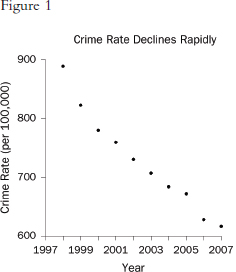
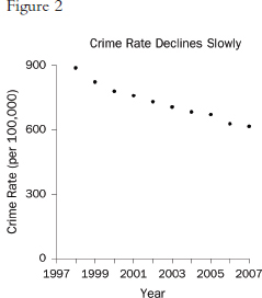
Graphs that plot values over time are useful for seeing trends. However, the scales on the axes matter. In Figure 1, the rate of all crimes of domestic violence in Florida (per 100,000 people) appears to decline rapidly over the 10 years from 1998 through 2007; in Figure 2, the same rate appears to drop slowly.65 The moral is simple: Pay attention to the markings on the axes to determine whether the scale is appropriate.
2. How are distributions displayed?
A graph commonly used to display the distribution of data is the histogram. One axis denotes the numbers, and the other indicates how often those fall within
65. Florida Statistical Analysis Center, Florida Department of Law Enforcement, Florida’s Crime Rate at a Glance, available at http://www.fdle.state.fl.us/FSAC/Crime_Trends/domestic_violence/index.asp. The data are from the Florida Uniform Crime Report statistics on crimes ranging from simple stalking and forcible fondling to murder and arson. The Web page with the numbers graphed in Figures 1 and 2 is no longer posted, but similar data for all violent crime is available at http://www.fdle.state.fl.us/FSAC/Crime_Trends/Violent-Crime.aspx.
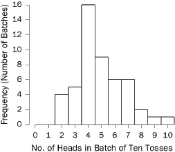
specified intervals (called “bins” or “class intervals”). For example, we flipped a quarter 10 times in a row and counted the number of heads in this “batch” of 10 tosses. With 50 batches, we obtained the following counts:66
7 7 5 6 8 4 2 3 6 5 4 3 4 7 4 6 8 4 7 4 7 4 5 4 3
4 4 2 5 3 5 4 2 4 4 5 7 2 3 5 4 6 4 9 10 5 5 6 6 4
The histogram is shown in Figure 3.67 A histogram shows how the data are distributed over the range of possible values. The spread can be made to appear larger or smaller, however, by changing the scale of the horizontal axis. Likewise, the shape can be altered somewhat by changing the size of the bins.68 It may be worth inquiring how the analyst chose the bin widths.
Figure 3. Histogram showing how frequently various numbers of heads appeared in 50 batches of 10 tosses of a quarter.
66. The coin landed heads 7 times in the first 10 tosses; by coincidence, there were also 7 heads in the next 10 tosses; there were 5 heads in the third batch of 10 tosses; and so forth.
67. In Figure 3, the bin width is 1. There were no 0s or 1s in the data, so the bars over 0 and 1 disappear. There is a bin from 1.5 to 2.5; the four 2s in the data fall into this bin, so the bar over the interval from 1.5 to 2.5 has height 4. There is another bin from 2.5 to 3.5, which catches five 3s; the height of the corresponding bar is 5. And so forth.
All the bins in Figure 3 have the same width, so this histogram is just like a bar graph. However, data are often published in tables with unequal intervals. The resulting histograms will have unequal bin widths; bar heights should be calculated so that the areas (height × width) are proportional to the frequencies. In general, a histogram differs from a bar graph in that it represents frequencies by area, not height. See Freedman et al., supra note 12, at 31–41.
68. As the width of the bins decreases, the graph becomes more detailed, but the appearance becomes more ragged until finally the graph is effectively a plot of each datum. The optimal bin width depends on the subject matter and the goal of the analysis.
D. Is an Appropriate Measure Used for the Center of a Distribution?
Perhaps the most familiar descriptive statistic is the mean (or “arithmetic mean”). The mean can be found by adding all the numbers and dividing the total by how many numbers were added. By comparison, the median cuts the numbers into halves: half the numbers are larger than the median and half are smaller.69 Yet a third statistic is the mode, which is the most common number in the dataset. These statistics are different, although they are not always clearly distinguished.70 The mean takes account of all the data—it involves the total of all the numbers; however, particularly with small datasets, a few unusually large or small observations may have too much influence on the mean. The median is resistant to such outliers.
Thus, studies of damage awards in tort cases find that the mean is larger than the median.71 This is because the mean takes into account (indeed, is heavily influenced by) the magnitudes of the relatively few very large awards, whereas the median merely counts their number. If one is seeking a single, representative number for the awards, the median may be more useful than the mean.72 Still, if the issue is whether insurers were experiencing more costs from jury verdicts, the mean is the more appropriate statistic: The total of the awards is directly related to the mean, not to the median.73
69. Technically, at least half the numbers are at the median or larger; at least half are at the median or smaller. When the distribution is symmetric, the mean equals the median. The values diverge, however, when the distribution is asymmetric, or skewed.
70. In ordinary language, the arithmetic mean, the median, and the mode seem to be referred to interchangeably as “the average.” In statistical parlance, however, the average is the arithmetic mean. The mode is rarely used by statisticians, because it is unstable: Small changes to the data often result in large changes to the mode.
71. In a study using a probability sample of cases, the median compensatory award in wrongful death cases was $961,000, whereas the mean award was around $3.75 million for the 162 cases in which the plaintiff prevailed. Thomas H. Cohen & Steven K. Smith, U.S. Dep’t of Justice, Bureau of Justice Statistics Bulletin NCJ 202803, Civil Trial Cases and Verdicts in Large Counties 2001, 10 (2004). In TXO Production Corp. v. Alliance Resources Corp., 509 U.S. 443 (1993), briefs portraying the punitive damage system as out of control pointed to mean punitive awards. These were some 10 times larger than the median awards described in briefs defending the system of punitive damages. Michael Rustad & Thomas Koenig, The Supreme Court and Junk Social Science: Selective Distortion in Amicus Briefs, 72 N.C. L. Rev. 91, 145–47 (1993).
72. In passing on proposed settlements in class-action lawsuits, courts have been advised to look to the magnitude of the settlements negotiated by the parties. But the mean settlement will be large if a higher number of meritorious, high-cost cases are resolved early in the life cycle of the litigation. This possibility led the court in In re Educational Testing Service Praxis Principles of Learning and Teaching, Grades 7-12 Litig., 447 F. Supp. 2d 612, 625 (E.D. La. 2006), to regard the smaller median settlement as “more representative of the value of a typical claim than the mean value” and to use this median in extrapolating to the entire class of pending claims.
73. To get the total award, just multiply the mean by the number of awards; by contrast, the total cannot be computed from the median. (The more pertinent figure for the insurance industry is
Research also has shown that there is considerable stability in the ratio of punitive to compensatory damage awards, and the Supreme Court has placed great weight on this ratio in deciding whether punitive damages are excessive in a particular case. In Exxon Shipping Co. v. Baker,74 Exxon contended that an award of $2.5 billion in punitive damages for a catastrophic oil spill in Alaska was unreasonable under federal maritime law. The Court looked to a “comprehensive study of punitive damages awarded by juries in state civil trials [that] found a median ratio of punitive to compensatory awards of just 0.62:1, but a mean ratio of 2.90:1.”75 The higher mean could reflect a relatively small but disturbing proportion of unjustifiably large punitive awards.76 Looking to the median ratio as “the line near which cases like this one largely should be grouped,” the majority concluded that “a 1:1 ratio, which is above the median award, is a fair upper limit in such maritime cases [of reckless conduct].”77
E. Is an Appropriate Measure of Variability Used?
The location of the center of a batch of numbers reveals nothing about the variations exhibited by these numbers.78 Statistical measures of variability include the range, the interquartile range, and the standard deviation. The range is the difference between the largest number in the batch and the smallest. The range seems natural, and it indicates the maximum spread in the numbers, but the range is unstable because it depends entirely on the most extreme values.79 The interquartile range is the difference between the 25th and 75th percentiles.80 The interquartile range contains 50% of the numbers and is resistant to changes in extreme values. The standard deviation is a sort of mean deviation from the mean.81
not the total of jury awards, but actual claims experience including settlements; of course, even the risk of large punitive damage awards may have considerable impact.)
74. 128 S. Ct. 2605 (2008).
75. Id. at 2625.
76. According to the Court, “the outlier cases subject defendants to punitive damages that dwarf the corresponding compensatories,” and the “stark unpredictability” of these rare awards is the “real problem.” Id. This perceived unpredictability has been the subject of various statistical studies and much debate. See Anthony J. Sebok, Punitive Damages: From Myth to Theory, 92 Iowa L. Rev. 957 (2007).
77. 128 S. Ct. at 2633.
78. The numbers 1, 2, 5, 8, 9 have 5 as their mean and median. So do the numbers 5, 5, 5, 5, 5. In the first batch, the numbers vary considerably about their mean; in the second, the numbers do not vary at all.
79. Moreover, the range typically depends on the number of units in the sample.
80. By definition, 25% of the data fall below the 25th percentile, 90% fall below the 90th percentile, and so on. The median is the 50th percentile.
81. When the distribution follows the normal curve, about 68% of the data will be within 1 standard deviation of the mean, and about 95% will be within 2 standard deviations of the mean. For other distributions, the proportions will be different.
There are no hard and fast rules about which statistic is the best. In general, the bigger the measures of spread are, the more the numbers are dispersed.82 Particularly in small datasets, the standard deviation can be influenced heavily by a few outlying values. To assess the extent of this influence, the mean and the standard deviation can be recomputed with the outliers discarded. Beyond this, any of the statistics can (and often should) be supplemented with a figure that displays much of the data.
IV. What Inferences Can Be Drawn from the Data?
The inferences that may be drawn from a study depend on the design of the study and the quality of the data (supra Section II). The data might not address the issue of interest, might be systematically in error, or might be difficult to interpret because of confounding. Statisticians would group these concerns together under the rubric of “bias.” In this context, bias means systematic error, with no connotation of prejudice. We turn now to another concern, namely, the impact of random chance on study results (“random error”).83
If a pattern in the data is the result of chance, it is likely to wash out when more data are collected. By applying the laws of probability, a statistician can assess the likelihood that random error will create spurious patterns of certain kinds. Such assessments are often viewed as essential when making inferences from data.
Technically, the standard deviation is the square root of the variance; the variance is the mean square deviation from the mean. For example, if the mean is 100, then 120 deviates from the mean by 20, and the square of 20 is 202 = 400. If the variance (i.e., the mean of the squared deviations) is 900, then the standard deviation is the square root of 900, that is, ![]() = 30. Taking the square root gets back to the original scale of the measurements. For example, if the measurements are of length in inches, the variance is in square inches; taking the square root changes back to inches.
= 30. Taking the square root gets back to the original scale of the measurements. For example, if the measurements are of length in inches, the variance is in square inches; taking the square root changes back to inches.
82. In Exxon Shipping Co. v. Baker, 554 U.S. 471 (2008), along with the mean and median ratios of punitive to compensatory awards of 0.62 and 2.90, the Court referred to a standard deviation of 13.81. Id. at 498. These numbers led the Court to remark that “[e]ven to those of us unsophisticated in statistics, the thrust of these figures is clear: the spread is great, and the outlier cases subject defendants to punitive damages that dwarf the corresponding compensatories.” Id. at 499-500. The size of the standard deviation compared to the mean supports the observation that ratios in the cases of jury award studies are dispersed. A graph of each pair of punitive and compensatory damages offers more insight into how scattered these figures are. See Theodore Eisenberg et al., The Predictability of Punitive Damages, 26 J. Legal Stud. 623 (1997); infra Section V.A (explaining scatter diagrams).
83. Random error is also called sampling error, chance error, or statistical error. Econometricians use the parallel concept of random disturbance terms. See Rubinfeld, supra note 21. Randomness and cognate terms have precise technical meanings; it is randomness in the technical sense that justifies the probability calculations behind standard errors, confidence intervals, and p-values (supra Section II.D, infra Sections IV.A–B). For a discussion of samples and populations, see supra Section II.B.
Thus, statistical inference typically involves tasks such as the following, which will be discussed in the rest of this guide.
- Estimation. A statistician draws a sample from a population (supra Section II.B) and estimates a parameter—that is, a numerical characteristic of the population. (The average value of a large group of claims is a parameter of perennial interest.) Random error will throw the estimate off the mark. The question is, by how much? The precision of an estimate is usually reported in terms of the standard error and a confidence interval.
- Significance testing. A “null hypothesis” is formulated—for example, that a parameter takes a particular value. Because of random error, an estimated value for the parameter is likely to differ from the value specified by the null—even if the null is right. (“Null hypothesis” is often shortened to “null.”) How likely is it to get a difference as large as, or larger than, the one observed in the data? This chance is known as a p-value. Small p-values argue against the null hypothesis. Statistical significance is determined by reference to the p-value; significance testing (also called hypothesis testing) is the technique for computing p-values and determining statistical significance.
- Developing a statistical model. Statistical inferences often depend on the validity of statistical models for the data. If the data are collected on the basis of a probability sample or a randomized experiment, there will be statistical models that suit the occasion, and inferences based on these models will be secure. Otherwise, calculations are generally based on analogy: This group of people is like a random sample; that observational study is like a randomized experiment. The fit between the statistical model and the data collection process may then require examination—how good is the analogy? If the model breaks down, that will bias the analysis.
- Computing posterior probabilities. Given the sample data, what is the probability of the null hypothesis? The question might be of direct interest to the courts, especially when translated into English; for example, the null hypothesis might be the innocence of the defendant in a criminal case. Posterior probabilities can be computed using a formula called Bayes’ rule. However, the computation often depends on prior beliefs about the statistical model and its parameters; such prior beliefs almost necessarily require subjective judgment. According to the frequentist theory of statistics,84
84. The frequentist theory is also called objectivist, by contrast with the subjectivist version of Bayesian theory. In brief, frequentist methods treat probabilities as objective properties of the system being studied. Subjectivist Bayesians view probabilities as measuring subjective degrees of belief. See infra Section IV.D and Appendix, Section A, for discussion of the two positions. The Bayesian position is named after the Reverend Thomas Bayes (England, c. 1701–1761). His essay on the subject was published after his death: An Essay Toward Solving a Problem in the Doctrine of Chances, 53 Phil. Trans. Royal Soc’y London 370 (1763–1764). For discussion of the foundations and varieties of Bayesian and
prior probabilities rarely have meaning and neither do posterior probabilities.85
Key ideas of estimation and testing will be illustrated by courtroom examples, with some complications omitted for ease of presentation and some details postponed (see infra Section V.D on statistical models, and the Appendix on the calculations).
The first example, on estimation, concerns the Nixon papers. Under the Presidential Recordings and Materials Preservation Act of 1974, Congress impounded Nixon’s presidential papers after he resigned. Nixon sued, seeking compensation on the theory that the materials belonged to him personally. Courts ruled in his favor: Nixon was entitled to the fair market value of the papers, with the amount to be proved at trial.86
The Nixon papers were stored in 20,000 boxes at the National Archives in Alexandria, Virginia. It was plainly impossible to value this entire population of material. Appraisers for the plaintiff therefore took a random sample of 500 boxes. (From this point on, details are simplified; thus, the example becomes somewhat hypothetical.) The appraisers determined the fair market value of each sample box. The average of the 500 sample values turned out to be $2000. The standard deviation (supra Section III.E) of the 500 sample values was $2200. Many boxes had low appraised values whereas some boxes were considered to be extremely valuable; this spread explains the large standard deviation.
1. What estimator should be used?
With the Nixon papers, it is natural to use the average value of the 500 sample boxes to estimate the average value of all 20,000 boxes comprising the population.
other forms of statistical inference, see, e.g., Richard M. Royall, Statistical Inference: A Likelihood Paradigm (1997); James Berger, The Case for Objective Bayesian Analysis, 1 Bayesian Analysis 385 (2006), available at http://ba.stat.cmu.edu/journal/2006/vol01/issue03/berger.pdf; Stephen E. Fienberg, Does It Make Sense to be an “Objective Bayesian”? (Comment on Articles by Berger and by Goldstein), 1 Bayesian Analysis 429 (2006); David Freedman, Some Issues in the Foundation of Statistics, 1 Found. Sci. 19 (1995), reprinted in Topics in the Foundation of Statistics 19 (Bas C. van Fraasen ed., 1997); see also D.H. Kaye, What Is Bayesianism? in Probability and Inference in the Law of Evidence: The Uses and Limits of Bayesianism (Peter Tillers & Eric Green eds., 1988), reprinted in 28 Jurimetrics J. 161 (1988) (distinguishing between “Bayesian probability,” “Bayesian statistical inference,” “Bayesian inference writ large,” and “Bayesian decision theory”).
85. Prior probabilities of repeatable events (but not hypotheses) can be defined within the frequentist framework. See infra note 122. When this happens, prior and posterior probabilities for these events are meaningful according to both schools of thought.
86. Nixon v. United States, 978 F.2d 1269 (D.C. Cir. 1992); Griffin v. United States, 935 F. Supp. 1 (D.D.C. 1995).
With the average value for each box having been estimated as $2000, the plaintiff demanded compensation in the amount of
20,000 × $2,000 = $40,000,000.
In more complex problems, statisticians may have to choose among several estimators. Generally, estimators that tend to make smaller errors are preferred; however, “error” might be quantified in more than one way. Moreover, the advantage of one estimator over another may depend on features of the population that are largely unknown, at least before the data are collected and analyzed. For complicated problems, professional skill and judgment may therefore be required when choosing a sample design and an estimator. In such cases, the choices and the rationale for them should be documented.
2. What is the standard error? The confidence interval?
An estimate based on a sample is likely to be off the mark, at least by a small amount, because of random error. The standard error gives the likely magnitude of this random error, with smaller standard errors indicating better estimates.87 In our example of the Nixon papers, the standard error for the sample average can be computed from (1) the size of the sample—500 boxes—and (2) the standard deviation of the sample values; see infra Appendix. Bigger samples give estimates that are more precise. Accordingly, the standard error should go down as the sample size grows, although the rate of improvement slows as the sample gets bigger. (“Sample size” and “the size of the sample” just mean the number of items in the sample; the “sample average” is the average value of the items in the sample.) The standard deviation of the sample comes into play by measuring heterogeneity. The less heterogeneity in the values, the smaller the standard error. For example, if all the values were about the same, a tiny sample would give an accurate estimate. Conversely, if the values are quite different from one another, a larger sample would be needed.
With a random sample of 500 boxes and a standard deviation of $2200, the standard error for the sample average is about $100. The plaintiff’s total demand was figured as the number of boxes (20,000) times the sample average ($2000). Therefore, the standard error for the total demand can be computed as 20,000 times the standard error for the sample average88:
87. We distinguish between (1) the standard deviation of the sample, which measures the spread in the sample data and (2) the standard error of the sample average, which measures the likely size of the random error in the sample average. The standard error is often called the standard deviation, and courts generally use the latter term. See, e.g., Castaneda v. Partida, 430 U.S. 482 (1977).
88. We are assuming a simple random sample. Generally, the formula for the standard error must take into account the method used to draw the sample and the nature of the estimator. In fact, the Nixon appraisers used more elaborate statistical procedures. Moreover, they valued the material as of
20,000 × $100 = $2,000,000.
How is the standard error to be interpreted? Just by the luck of the draw, a few too many high-value boxes may have come into the sample, in which case the estimate of $40,000,000 is too high. Or, a few too many low-value boxes may have been drawn, in which case the estimate is too low. This is random error. The net effect of random error is unknown, because data are available only on the sample, not on the full population. However, the net effect is likely to be something close to the standard error of $2,000,000. Random error throws the estimate off, one way or the other, by something close to the standard error. The role of the standard error is to gauge the likely size of the random error.
The plaintiff’s argument may be open to a variety of objections, particularly regarding appraisal methods. However, the sampling plan is sound, as is the extrapolation from the sample to the population. And there is no need for a larger sample: The standard error is quite small relative to the total claim.
Random errors larger in magnitude than the standard error are commonplace. Random errors larger in magnitude than two or three times the standard error are unusual. Confidence intervals make these ideas more precise. Usually, a confidence interval for the population average is centered at the sample average; the desired confidence level is obtained by adding and subtracting a suitable multiple of the standard error. Statisticians who say that the population average falls within 1 standard error of the sample average will be correct about 68% of the time. Those who say “within 2 standard errors” will be correct about 95% of the time, and those who say “within 3 standard errors” will be correct about 99.7% of the time, and so forth. (We are assuming a large sample; the confidence levels correspond to areas under the normal curve and are approximations; the “population average” just means the average value of all the items in the population.89) In summary,
- To get a 68% confidence interval, start at the sample average, then add and subtract 1 standard error.
- To get a 95% confidence interval, start at the sample average, then add and subtract twice the standard error.
1995, extrapolated backward to the time of taking (1974), and then added interest. The text ignores these complications.
89. See infra Appendix. The area under the normal curve between −1 and +1 is close to 68.3%. Likewise, the area between −2 and +2 is close to 95.4%. Many academic statisticians would use ±1.96 SE for a 95% confidence interval. However, the normal curve only gives an approximation to the relevant chances, and the error in that approximation will often be larger than a few tenths of a percent. For simplicity, we use ±1 SE for the 68% confidence level, and ±2 SE for 95% confidence. The normal curve gives good approximations when the sample size is reasonably large; for small samples, other techniques should be used. See infra notes 106–07.
- To get a 99.7% confidence interval, start at the sample average, then add and subtract three times the standard error.
With the Nixon papers, the 68% confidence interval for plaintiff’s total demand runs
from $40,000,000 - $2,000,000 = $38,000,000
to $40,000,000 + $2,000,000 = $42,000,000.
The 95% confidence interval runs
from $40,000,000 - (2 × $2,000,000) = $36,000,000
to $40,000,000 + (2 × $2,000,000) = $44,000,000.
The 99.7% confidence interval runs
from $40,000,000 - (3 × $2,000,000) = $34,000,000
to $40,000,000 + (3 × $2,000,000) = $46,000,000.
To write this more compactly, we abbreviate standard error as SE. Thus, 1 SE is one standard error, 2 SE is twice the standard error, and so forth. With a large sample and an estimate like the sample average, a 68% confidence interval is the range
estimate − 1 SE to estimate + 1 SE.
A 95% confidence interval is the range
estimate − 2 SE to estimate + 2 SE.
The 99.7% confidence interval is the range
estimate − 3 SE to estimate + 3 SE.
For a given sample size, increased confidence can be attained only by widening the interval. The 95% confidence level is the most popular, but some authors use 99%, and 90% is seen on occasion. (The corresponding multipliers on the SE are about 2, 2.6, and 1.6, respectively; see infra Appendix.) The phrase “margin of error” generally means twice the standard error. In medical journals, “confidence interval” is often abbreviated as “CI.”
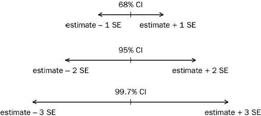
The main point is that an estimate based on a sample will differ from the exact population value, because of random error. The standard error gives the likely size of the random error. If the standard error is small, random error probably has little effect. If the standard error is large, the estimate may be seriously wrong. Confidence intervals are a technical refinement, and bias is a separate issue to consider (infra Section IV.A.4).
3. How big should the sample be?
There is no easy answer to this sensible question. Much depends on the level of error that is tolerable and the nature of the material being sampled. Generally, increasing the size of the sample will reduce the level of random error (“sampling error”). Bias (“nonsampling error”) cannot be reduced that way. Indeed, beyond some point, large samples are harder to manage and more vulnerable to nonsampling error. To reduce bias, the researcher must improve the design of the study or use a statistical model more tightly linked to the data collection process.
If the material being sampled is heterogeneous, random error will be large; a larger sample will be needed to offset the heterogeneity (supra Section IV.A.1). A pilot sample may be useful to estimate heterogeneity and determine the final sample size. Probability samples require some effort in the design phase, and it will rarely be sensible to draw a sample with fewer than, say, two or three dozen items. Moreover, with such small samples, methods based on the normal curve (supra Section IV.A.2) will not apply.
Population size (i.e., the number of items in the population) usually has little bearing on the precision of estimates for the population average. This is surprising. On the other hand, population size has a direct bearing on estimated totals. Both points are illustrated by the Nixon papers (see supra Section IV.A.2 and infra Appendix). To be sure, drawing a probability sample from a large population may
involve a lot of work. Samples presented in the courtroom have ranged from 5 (tiny) to 1.7 million (huge).90
4. What are the technical difficulties?
To begin with, “confidence” is a term of art. The confidence level indicates the percentage of the time that intervals from repeated samples would cover the true value. The confidence level does not express the chance that repeated estimates would fall into the confidence interval.91 With the Nixon papers, the 95% confidence interval should not be interpreted as saying that 95% of all random samples will produce estimates in the range from $36 million to $44 million. Moreover, the confidence level does not give the probability that the unknown parameter lies within the confidence interval.92 For example, the 95% confidence level should not be translated to a 95% probability that the total value of the papers is in the range from $36 million to $44 million. According to the frequentist theory of statistics, probability statements cannot be made about population characteristics: Probability statements apply to the behavior of samples. That is why the different term “confidence” is used.
The next point to make is that for a given confidence level, a narrower interval indicates a more precise estimate, whereas a broader interval indicates less
90. See Lebrilla v. Farmers Group, Inc., No. 00-CC-017185 (Cal. Super. Ct., Orange County, Dec. 5, 2006) (preliminary approval of settlement), a class action lawsuit on behalf of plaintiffs who were insured by Farmers and had automobile accidents. Plaintiffs alleged that replacement parts recommended by Farmers did not meet specifications: Small samples were used to evaluate these allegations. At the other extreme, it was proposed to adjust Census 2000 for undercount and overcount by reviewing a sample of 1.7 million persons. See Brown et al., supra note 29, at 353.
91. Opinions reflecting this misinterpretation include In re Silicone Gel Breast Implants Prods. Liab. Litig, 318 F. Supp. 2d 879, 897 (C.D. Cal. 2004) (“a margin of error between 0.5 and 8.0 at the 95% confidence level…means that 95 times out of 100 a study of that type would yield a relative risk value somewhere between 0.5 and 8.0.”); United States ex rel. Free v. Peters, 806 F. Supp. 705, 713 n.6 (N.D. Ill. 1992) (“A 99% confidence interval, for instance, is an indication that if we repeated our measurement 100 times under identical conditions, 99 times out of 100 the point estimate derived from the repeated experimentation will fall within the initial interval estimate….”), rev’d in part, 12 F.3d 700 (7th Cir. 1993). The more technically correct statement in the Silicone Gel case, for example, would be that “the confidence interval of 0.5 to 8.0 means that the relative risk in the population could fall within this wide range and that in roughly 95 times out of 100, random samples from the same population, the confidence intervals (however wide they might be) would include the population value (whatever it is).”
92. See, e.g., Freedman et al., supra note 12, at 383–86; infra Section IV.B.1. Consequently, it is misleading to suggest that “[a] 95% confidence interval means that there is a 95% probability that the ‘true’ relative risk falls within the interval” or that “the probability that the true value was…within two standard deviations of the mean…would be 95 percent.” DeLuca v. Merrell Dow Pharms., Inc., 791 F. Supp. 1042, 1046 (D.N.J. 1992), aff’d, 6 F.3d 778 (3d Cir. 1993); SmithKline Beecham Corp. v. Apotex Corp., 247 F. Supp. 2d 1011, 1037 (N.D. Ill. 2003), aff’d on other grounds, 403 F.3d 1331 (Fed. Cir. 2005).
precision.93 A high confidence level with a broad interval means very little, but a high confidence level for a small interval is impressive, indicating that the random error in the sample estimate is low. For example, take a 95% confidence interval for a damage claim. An interval that runs from $34 million to $44 million is one thing, but −$10 million to $90 million is something else entirely. Statements about confidence without mention of an interval are practically meaningless.94
Standard errors and confidence intervals are often derived from statistical models for the process that generated the data. The model usually has parameters—numerical constants describing the population from which samples were drawn. When the values of the parameters are not known, the statistician must work backward, using the sample data to make estimates. That was the case here.95 Generally, the chances needed for statistical inference are computed from a model and estimated parameter values.
If the data come from a probability sample or a randomized controlled experiment (supra Sections II.A–B), the statistical model may be connected tightly to the actual data collection process. In other situations, using the model may be tantamount to assuming that a sample of convenience is like a random sample, or that an observational study is like a randomized experiment. With the Nixon papers, the appraisers drew a random sample, and that justified the statistical
93. In Cimino v. Raymark Industries, Inc., 751 F. Supp. 649 (E.D. Tex. 1990), rev’d, 151 F.3d 297 (5th Cir. 1998), the district court drew certain random samples from more than 6000 pending asbestos cases, tried these cases, and used the results to estimate the total award to be given to all plaintiffs in the pending cases. The court then held a hearing to determine whether the samples were large enough to provide accurate estimates. The court’s expert, an educational psychologist, testified that the estimates were accurate because the samples matched the population on such characteristics as race and the percentage of plaintiffs still alive. Id. at 664. However, the matches occurred only in the sense that population characteristics fell within 99% confidence intervals computed from the samples. The court thought that matches within the 99% confidence intervals proved more than matches within 95% intervals. Id. This is backward. To be correct in a few instances with a 99% confidence interval is not very impressive—by definition, such intervals are broad enough to ensure coverage 99% of the time.
94. In Hilao v. Estate of Marcos, 103 F.3d 767 (9th Cir. 1996), for example, “an expert on statistics…testified that…a random sample of 137 claims would achieve ‘a 95% statistical probability that the same percentage determined to be valid among the examined claims would be applicable to the totality of [9541 facially valid] claims filed.’” Id. at 782. There is no 95% “statistical probability” that a percentage computed from a sample will be “applicable” to a population. One can compute a confidence interval from a random sample and be 95% confident that the interval covers some parameter. The computation can be done for a sample of virtually any size, with larger samples giving smaller intervals. What is missing from the opinion is a discussion of the widths of the relevant intervals. For the same reason, it is meaningless to testify, as an expert did in Ayyad v. Sprint Spectrum, L.P., No. RG03-121510 (Cal. Super. Ct., Alameda County) (transcript, May 28, 2008, at 730), that a simple regression equation is trustworthy because the coefficient of the explanatory variable has “an extremely high indication of reliability to more than 99% confidence level.”
95. With the Nixon papers, one parameter is the average value of all 20,000 boxes, and another parameter is the standard deviation of the 20,000 values. These parameters can be used to approximate the distribution of the sample average. See infra Appendix. Regression models and their parameters are discussed infra Section V and in Rubinfeld, supra note 21.
calculations—if not the appraised values themselves. In many contexts, the choice of an appropriate statistical model is less than obvious. When a model does not fit the data collection process, estimates and standard errors will not be probative.
Standard errors and confidence intervals generally ignore systematic errors such as selection bias or nonresponse bias (supra Sections II.B.1–2). For example, after reviewing studies to see whether a particular drug caused birth defects, a court observed that mothers of children with birth defects may be more likely to remember taking a drug during pregnancy than mothers with normal children. This selective recall would bias comparisons between samples from the two groups of women. The standard error for the estimated difference in drug usage between the groups would ignore this bias, as would the confidence interval.96
B. Significance Levels and Hypothesis Tests
In 1969, Dr. Benjamin Spock came to trial in the U.S. District Court for Massachusetts. The charge was conspiracy to violate the Military Service Act. The jury was drawn from a panel of 350 persons selected by the clerk of the court. The panel included only 102 women—substantially less than 50%—although a majority of the eligible jurors in the community were female. The shortfall in women was especially poignant in this case: “Of all defendants, Dr. Spock, who had given wise and welcome advice on child-rearing to millions of mothers, would have liked women on his jury.”97
Can the shortfall in women be explained by the mere play of random chance? To approach the problem, a statistician would formulate and test a null hypothesis. Here, the null hypothesis says that the panel is like 350 persons drawn at random from a large population that is 50% female. The expected number of women drawn would then be 50% of 350, which is 175. The observed number of women is 102. The shortfall is 175 - 102 = 73. How likely is it to find a disparity this large or larger, between observed and expected values? The probability is called p, or the p-value.
96. Brock v. Merrell Dow Pharms., Inc., 874 F.2d 307, 311–12 (5th Cir.), modified, 884 F.2d 166 (5th Cir. 1989). In Brock, the court stated that the confidence interval took account of bias (in the form of selective recall) as well as random error. 874 F.2d at 311–12. This is wrong. Even if the sampling error were nonexistent—which would be the case if one could interview every woman who had a child during the period that the drug was available—selective recall would produce a difference in the percentages of reported drug exposure between mothers of children with birth defects and those with normal children. In this hypothetical situation, the standard error would vanish. Therefore, the standard error could disclose nothing about the impact of selective recall.
97. Hans Zeisel, Dr. Spock and the Case of the Vanishing Women Jurors, 37 U. Chi. L. Rev. 1 (1969). Zeisel’s reasoning was different from that presented in this text. The conviction was reversed on appeal without reaching the issue of jury selection. United States v. Spock, 416 F.2d 165 (1st Cir. 1965).
The p-value is the probability of getting data as extreme as, or more extreme than, the actual data—given that the null hypothesis is true. In the example, p turns out to be essentially zero. The discrepancy between the observed and the expected is far too large to explain by random chance. Indeed, even if the panel had included 155 women, the p-value would only be around 0.02, or 2%.98 (If the population is more than 50% female, p will be even smaller.) In short, the jury panel was nothing like a random sample from the community.
Large p-values indicate that a disparity can easily be explained by the play of chance: The data fall within the range likely to be produced by chance variation. On the other hand, if p is very small, something other than chance must be involved: The data are far away from the values expected under the null hypothesis. Significance testing often seems to involve multiple negatives. This is because a statistical test is an argument by contradiction.
With the Dr. Spock example, the null hypothesis asserts that the jury panel is like a random sample from a population that is 50% female. The data contradict this null hypothesis because the disparity between what is observed and what is expected (according to the null) is too large to be explained as the product of random chance. In a typical jury discrimination case, small p-values help a defendant appealing a conviction by showing that the jury panel is not like a random sample from the relevant population; large p-values hurt. In the usual employment context, small p-values help plaintiffs who complain of discrimination—for example, by showing that a disparity in promotion rates is too large to be explained by chance; conversely, large p-values would be consistent with the defense argument that the disparity is just due to chance.
Because p is calculated by assuming that the null hypothesis is correct, p does not give the chance that the null is true. The p-value merely gives the chance of getting evidence against the null hypothesis as strong as or stronger than the evidence at hand. Chance affects the data, not the hypothesis. According to the frequency theory of statistics, there is no meaningful way to assign a numerical probability to the null hypothesis. The correct interpretation of the p-value can therefore be summarized in two lines:
p is the probability of extreme data given the null hypothesis.
p is not the probability of the null hypothesis given extreme data.99
98. With 102 women out of 350, the p-value is about 2/1015, where 1015 is 1 followed by 15 zeros, that is, a quadrillion. See infra Appendix for the calculations.
99. Some opinions present a contrary view. E.g., Vasquez v. Hillery, 474 U.S. 254, 259 n.3 (1986) (“the District Court…ultimately accepted…a probability of 2 in 1000 that the phenomenon was attributable to chance”); Nat’l Abortion Fed. v. Ashcroft, 330 F. Supp. 2d 436 (S.D.N.Y. 2004), aff’d in part, 437 F.3d 278 (2d Cir. 2006), vacated, 224 Fed. App’x. 88 (2d Cir. 2007) (“According to Dr. Howell,…a ‘P value’ of 0.30…indicates that there is a thirty percent probability that the results of the…[s]tudy were merely due to chance alone.”). Such statements confuse the probability of the
To recapitulate the logic of significance testing: If p is small, the observed data are far from what is expected under the null hypothesis—too far to be readily explained by the operations of chance. That discredits the null hypothesis.
Computing p-values requires statistical expertise. Many methods are available, but only some will fit the occasion. Sometimes standard errors will be part of the analysis; other times they will not be. Sometimes a difference of two standard errors will imply a p-value of about 5%; other times it will not. In general, the p-value depends on the model, the size of the sample, and the sample statistics.
2. Is a difference statistically significant?
If an observed difference is in the middle of the distribution that would be expected under the null hypothesis, there is no surprise. The sample data are of the type that often would be seen when the null hypothesis is true. The difference is not significant, as statisticians say, and the null hypothesis cannot be rejected. On the other hand, if the sample difference is far from the expected value—according to the null hypothesis—then the sample is unusual. The difference is significant, and the null hypothesis is rejected. Statistical significance is determined by comparing p to a preset value, called the significance level.100 The null hypothesis is rejected when p falls below this level.
In practice, statistical analysts typically use levels of 5% and 1%.101 The 5% level is the most common in social science, and an analyst who speaks of significant results without specifying the threshold probably is using this figure. An unexplained reference to highly significant results probably means that p is less
kind of outcome observed, which is computed under some model of chance, with the probability that chance is the explanation for the outcome—the “transposition fallacy.”
100. Statisticians use the Greek letter alpha (a) to denote the significance level; a gives the chance of getting a significant result, assuming that the null hypothesis is true. Thus, a represents the chance of a false rejection of the null hypothesis (also called a false positive, a false alarm, or a Type I error). For example, suppose a = 5%. If investigators do many studies, and the null hypothesis happens to be true in each case, then about 5% of the time they would obtain significant results—and falsely reject the null hypothesis.
101. The Supreme Court implicitly referred to this practice in Castaneda v. Partida, 430 U.S. 482, 496 n.17 (1977), and Hazelwood School District v. United States, 433 U.S. 299, 311 n.17 (1977). In these footnotes, the Court described the null hypothesis as “suspect to a social scientist” when a statistic from “large samples” falls more than “two or three standard deviations” from its expected value under the null hypothesis. Although the Court did not say so, these differences produce p-values of about 5% and 0.3% when the statistic is normally distributed. The Court’s standard deviation is our standard error.
than 1%. These levels of 5% and 1% have become icons of science and the legal process. In truth, however, such levels are at best useful conventions.
Because the term “significant” is merely a label for a certain kind of p-value, significance is subject to the same limitations as the underlying p-value. Thus, significant differences may be evidence that something besides random error is at work. They are not evidence that this something is legally or practically important. Statisticians distinguish between statistical and practical significance to make the point. When practical significance is lacking—when the size of a disparity is negligible—there is no reason to worry about statistical significance.102
It is easy to mistake the p-value for the probability of the null hypothesis given the data (supra Section IV.B.1). Likewise, if results are significant at the 5% level, it is tempting to conclude that the null hypothesis has only a 5% chance of being correct.103 This temptation should be resisted. From the frequentist perspective, statistical hypotheses are either true or false. Probabilities govern the samples, not the models and hypotheses. The significance level tells us what is likely to happen when the null hypothesis is correct; it does not tell us the probability that the hypothesis is true. Significance comes no closer to expressing the probability that the null hypothesis is true than does the underlying p-value.
3. Tests or interval estimates?
How can a highly significant difference be practically insignificant? The reason is simple: p depends not only on the magnitude of the effect, but also on the sample size (among other things). With a huge sample, even a tiny effect will be
102. E.g., Waisome v. Port Auth., 948 F.2d 1370, 1376 (2d Cir. 1991) (“though the disparity was found to be statistically significant, it was of limited magnitude.”); United States v. Henderson, 409 F.3d 1293, 1306 (11th Cir. 2005) (regardless of statistical significance, excluding law enforcement officers from jury service does not have a large enough impact on the composition of grand juries to violate the Jury Selection and Service Act); cf. Thornburg v. Gingles, 478 U.S. 30, 53–54 (1986) (repeating the district court’s explanation of why “the correlation between the race of the voter and the voter’s choice of certain candidates was [not only] statistically significant,” but also “so marked as to be substantively significant, in the sense that the results of the individual election would have been different depending upon whether it had been held among only the white voters or only the black voters.”).
103. E.g., Waisome, 948 F.2d at 1376 (“Social scientists consider a finding of two standard deviations significant, meaning there is about one chance in 20 that the explanation for a deviation could be random….”); Adams v. Ameritech Serv., Inc., 231 F.3d 414, 424 (7th Cir. 2000) (“Two standard deviations is normally enough to show that it is extremely unlikely (…less than a 5% probability) that the disparity is due to chance”); Magistrini v. One Hour Martinizing Dry Cleaning, 180 F. Supp. 2d 584, 605 n.26 (D.N.J. 2002) (a “statistically significant…study shows that there is only 5% probability that an observed association is due to chance.”); cf. Giles v. Wyeth, Inc., 500 F. Supp. 2d 1048, 1056 (S.D. Ill. 2007) (“While [plaintiff] admits that a p-value of .15 is three times higher than what scientists generally consider statistically significant—that is, a p-value of .05 or lower—she maintains that this “represents 85% certainty, which meets any conceivable concept of preponderance of the evidence.”).
highly significant.104 For example, suppose that a company hires 52% of male job applicants and 49% of female applicants. With a large enough sample, a statistician could compute an impressively small p-value. This p-value would confirm that the difference does not result from chance, but it would not convert a trivial difference (52% versus 49%) into a substantial one.105 In short, the p-value does not measure the strength or importance of an association.
A “significant” effect can be small. Conversely, an effect that is “not significant” can be large. By inquiring into the magnitude of an effect, courts can avoid being misled by p-values. To focus attention on more substantive concerns—the size of the effect and the precision of the statistical analysis—interval estimates (e.g., confidence intervals) may be more valuable than tests. Seeing a plausible range of values for the quantity of interest helps describe the statistical uncertainty in the estimate.
4. Is the sample statistically significant?
Many a sample has been praised for its statistical significance or blamed for its lack thereof. Technically, this makes little sense. Statistical significance is about the difference between observations and expectations. Significance therefore applies to statistics computed from the sample, but not to the sample itself, and certainly not to the size of the sample. Findings can be statistically significant. Differences can be statistically significant (supra Section IV.B.2). Estimates can be statistically significant (infra Section V.D.2). By contrast, samples can be representative or unrepresentative. They can be chosen well or badly (supra Section II.B.1). They can be large enough to give reliable results or too small to bother with (supra Section IV.A.3). But samples cannot be “statistically significant,” if this technical phrase is to be used as statisticians use it.
C. Evaluating Hypothesis Tests
1. What is the power of the test?
When a p-value is high, findings are not significant, and the null hypothesis is not rejected. This could happen for at least two reasons:
104. See supra Section IV.B.2. Although some opinions seem to equate small p-values with “gross” or “substantial” disparities, most courts recognize the need to decide whether the underlying sample statistics reveal that a disparity is large. E.g., Washington v. People, 186 P.3d 594 (Colo. 2008) (jury selection).
105. Cf. Frazier v. Garrison Indep. Sch. Dist., 980 F.2d 1514, 1526 (5th Cir. 1993) (rejecting claims of intentional discrimination in the use of a teacher competency examination that resulted in retention rates exceeding 95% for all groups); Washington, 186 P.2d 594 (although a jury selection practice that reduced the representation of “African-Americans [from] 7.7 percent of the population [to] 7.4 percent of the county’s jury panels produced a highly statistically significant disparity, the small degree of exclusion was not constitutionally significant.”).
- The null hypothesis is true.
- The null is false—but, by chance, the data happened to be of the kind expected under the null.
If the power of a statistical study is low, the second explanation may be plausible. Power is the chance that a statistical test will declare an effect when there is an effect to be declared.106 This chance depends on the size of the effect and the size of the sample. Discerning subtle differences requires large samples; small samples may fail to detect substantial differences.
When a study with low power fails to show a significant effect, the results may therefore be more fairly described as inconclusive than negative. The proof is weak because power is low. On the other hand, when studies have a good chance of detecting a meaningful association, failure to obtain significance can be persuasive evidence that there is nothing much to be found.107
For simplicity, the examples of statistical inference discussed here (supra Sections IV.A–B) were based on large samples. Small samples also can provide useful
106. More precisely, power is the probability of rejecting the null hypothesis when the alternative hypothesis (infra Section IV.C.5) is right. Typically, this probability will depend on the values of unknown parameters, as well as the preset significance level α. The power can be computed for any value of a and any choice of parameters satisfying the alternative hypothesis. See infra Appendix for an example. Frequentist hypothesis testing keeps the risk of a false positive to a specified level (such as α = 5%) and then tries to maximize power.
Statisticians usually denote power by the Greek letter beta (β). However, some authors use β to denote the probability of accepting the null hypothesis when the alternative hypothesis is true; this usage is fairly standard in epidemiology. Accepting the null hypothesis when the alternative holds true is a false negative (also called a Type II error, a missed signal, or a false acceptance of the null hypothesis).
The chance of a false negative may be computed from the power. Some commentators have claimed that the cutoff for significance should be chosen to equalize the chance of a false positive and a false negative, on the ground that this criterion corresponds to the more-probable-than-not burden of proof. The argument is fallacious, because α and β do not give the probabilities of the null and alternative hypotheses; see supra Sections IV.B.1–2; supra note 34. See also D.H. Kaye, Hypothesis Testing in the Courtroom, in Contributions to the Theory and Application of Statistics: A Volume in Honor of Herbert Solomon 331, 341–43 (Alan E. Gelfand ed., 1987).
107. Some formal procedures (meta-analysis) are available to aggregate results across studies. See, e.g., In re Bextra and Celebrex Marketing Sales Practices and Prod. Liab. Litig., 524 F. Supp. 2d 1166, 1174, 1184 (N.D. Cal. 2007) (holding that “[a] meta-analysis of all available published and unpublished randomized clinical trials” of certain pain-relief medicine was admissible). In principle, the power of the collective results will be greater than the power of each study. However, these procedures have their own weakness. See, e.g., Richard A. Berk & David A. Freedman, Statistical Assumptions as Empirical Commitments, in Punishment and Social Control: Essays in Honor of Sheldon Messinger 235, 244–48 (T.G. Blomberg & S. Cohen eds., 2d ed. 2003); Michael Oakes, Statistical Inference: A Commentary for the Social and Behavioral Sciences (1986); Diana B. Petitti, Meta-Analysis, Decision Analysis, and Cost-Effectiveness Analysis Methods for Quantitative Synthesis in Medicine (2d ed. 2000).
information. Indeed, when confidence intervals and p-values can be computed, the interpretation is the same with small samples as with large ones.108 The concern with small samples is not that they are beyond the ken of statistical theory, but that
- The underlying assumptions are hard to validate.
- Because approximations based on the normal curve generally cannot be used, confidence intervals may be difficult to compute for parameters of interest. Likewise, p-values may be difficult to compute for hypotheses of interest.109
- Small samples may be unreliable, with large standard errors, broad confidence intervals, and tests having low power.
In many cases, a statistical test can be done either one-tailed or two-tailed; the second method often produces a p-value twice as big as the first method. The methods are easily explained with a hypothetical example. Suppose we toss a coin 1000 times and get 532 heads. The null hypothesis to be tested asserts that the coin is fair. If the null is correct, the chance of getting 532 or more heads is 2.3%. That is a one-tailed test, whose p-value is 2.3%. To make a two-tailed test, the statistician computes the chance of getting 532 or more heads—or 500 - 32 = 468 heads or fewer. This is 4.6%. In other words, the two-tailed p-value is 4.6%. Because small p-values are evidence against the null hypothesis, the one-tailed test seems to produce stronger evidence than its two-tailed counterpart. However, the advantage is largely illusory, as the example suggests. (The two-tailed test may seem artificial, but it offers some protection against possible artifacts resulting from multiple testing—the topic of the next section.)
Some courts and commentators have argued for one or the other type of test, but a rigid rule is not required if significance levels are used as guidelines rather than as mechanical rules for statistical proof.110 One-tailed tests often make it
108. Advocates sometimes contend that samples are “too small to allow for meaningful statistical analysis,” United States v. New York City Bd. of Educ., 487 F. Supp. 2d 220, 229 (E.D.N.Y. 2007), and courts often look to the size of samples from earlier cases to determine whether the sample data before them are admissible or convincing. Id. at 230; Timmerman v. U.S. Bank, 483 F.3d 1106, 1116 n.4 (10th Cir. 2007). However, a meaningful statistical analysis yielding a significant result can be based on a small sample, and reliability does not depend on sample size alone (see supra Section IV.A.3, infra Section V.C.1). Well-known small-sample techniques include the sign test and Fisher’s exact test. E.g., Michael O. Finkelstein & Bruce Levin, Statistics for Lawyers 154–56, 339–41 (2d ed. 2001); see generally E.L. Lehmann & H.J.M. d’Abrera, Nonparametrics (2d ed. 2006).
109. With large samples, approximate inferences (e.g., based on the central limit theorem, see infra Appendix) may be quite adequate. These approximations will not be satisfactory for small samples.
110. See, e.g., United States v. State of Delaware, 93 Fair Empl. Prac. Cas. (BNA) 1248, 2004 WL 609331, *10 n.4 (D. Del. 2004). According to formal statistical theory, the choice between one
easier to reach a threshold such as 5%, at least in terms of appearance. However, if we recognize that 5% is not a magic line, then the choice between one tail and two is less important—as long as the choice and its effect on the p-value are made explicit.
4. How many tests have been done?
Repeated testing complicates the interpretation of significance levels. If enough comparisons are made, random error almost guarantees that some will yield “significant” findings, even when there is no real effect. To illustrate the point, consider the problem of deciding whether a coin is biased. The probability that a fair coin will produce 10 heads when tossed 10 times is (1/2)10 = 1/1024. Observing 10 heads in the first 10 tosses, therefore, would be strong evidence that the coin is biased. Nonetheless, if a fair coin is tossed a few thousand times, it is likely that at least one string of ten consecutive heads will appear. Ten heads in the first ten tosses means one thing; a run of ten heads somewhere along the way to a few thousand tosses of a coin means quite another. A test—looking for a run of ten heads—can be repeated too often.
Artifacts from multiple testing are commonplace. Because research that fails to uncover significance often is not published, reviews of the literature may produce an unduly large number of studies finding statistical significance.111 Even a single researcher may examine so many different relationships that a few will achieve statistical significance by mere happenstance. Almost any large dataset—even pages from a table of random digits—will contain some unusual pattern that can be uncovered by diligent search. Having detected the pattern, the analyst can perform a statistical test for it, blandly ignoring the search effort. Statistical significance is bound to follow.
There are statistical methods for dealing with multiple looks at the data, which permit the calculation of meaningful p-values in certain cases.112 However, no general solution is available, and the existing methods would be of little help in the typical case where analysts have tested and rejected a variety of models before arriving at the one considered the most satisfactory (see infra Section V on regression models). In these situations, courts should not be overly impressed with
tail or two can sometimes be made by considering the exact form of the alternative hypothesis (infra Section IV.C.5). But see Freedman et al., supra note 12, at 547–50. One-tailed tests at the 5% level are viewed as weak evidence—no weaker standard is commonly used in the technical literature. One-tailed tests are also called one-sided (with no pejorative intent); two-tailed tests are two-sided.
111. E.g., Philippa J. Easterbrook et al., Publication Bias in Clinical Research, 337 Lancet 867 (1991); John P.A. Ioannidis, Effect of the Statistical Significance of Results on the Time to Completion and Publication of Randomized Efficacy Trials, 279 JAMA 281 (1998); Stuart J. Pocock et al., Statistical Problems in the Reporting of Clinical Trials: A Survey of Three Medical Journals, 317 New Eng. J. Med. 426 (1987).
112. See, e.g., Sandrine Dudoit & Mark J. van der Laan, Multiple Testing Procedures with Applications to Genomics (2008).
claims that estimates are significant. Instead, they should be asking how analysts developed their models.113
5. What are the rival hypotheses?
The p-value of a statistical test is computed on the basis of a model for the data: the null hypothesis. Usually, the test is made in order to argue for the alternative hypothesis: another model. However, on closer examination, both models may prove to be unreasonable. A small p-value means something is going on besides random error. The alternative hypothesis should be viewed as one possible explanation, out of many, for the data.
In Mapes Casino, Inc. v. Maryland Casualty Co.,114 the court recognized the importance of explanations that the proponent of the statistical evidence had failed to consider. In this action to collect on an insurance policy, Mapes sought to quantify its loss from theft. It argued that employees were using an intermediary to cash in chips at other casinos. The casino established that over an 18-month period, the win percentage at its craps tables was 6%, compared to an expected value of 20%. The statistics proved that something was wrong at the craps tables—the discrepancy was too big to explain as the product of random chance. But the court was not convinced by plaintiff’s alternative hypothesis. The court pointed to other possible explanations (Runyonesque activities such as skimming, scamming, and crossroading) that might have accounted for the discrepancy without implicating the suspect employees.115 In short, rejection of the null hypothesis does not leave the proffered alternative hypothesis as the only viable explanation for the data.116
113. Intuition may suggest that the more variables included in the model, the better. However, this idea often turns out to be wrong. Complex models may reflect only accidental features of the data. Standard statistical tests offer little protection against this possibility when the analyst has tried a variety of models before settling on the final specification. See authorities cited, supra note 21.
114. 290 F. Supp. 186 (D. Nev. 1968).
115. Id. at 193. Skimming consists of “taking off the top before counting the drop,” scamming is “cheating by collusion between dealer and player,” and crossroading involves “professional cheaters among the players.” Id. In plainer language, the court seems to have ruled that the casino itself might be cheating, or there could have been cheaters other than the particular employees identified in the case. At the least, plaintiff’s statistical evidence did not rule out such possibilities. Compare EEOC v. Sears, Roebuck & Co., 839 F.2d 302, 312 & n.9, 313 (7th Cir. 1988) (EEOC’s regression studies showing significant differences did not establish liability because surveys and testimony supported the rival hypothesis that women generally had less interest in commission sales positions), with EEOC v. General Tel. Co., 885 F.2d 575 (9th Cir. 1989) (unsubstantiated rival hypothesis of “lack of interest” in “nontraditional” jobs insufficient to rebut prima facie case of gender discrimination); cf. supra Section II.A (problem of confounding).
116. E.g., Coleman v. Quaker Oats Co., 232 F.3d 1271, 1283 (9th Cir. 2000) (a disparity with a p-value of “3 in 100 billion” did not demonstrate age discrimination because “Quaker never contends that the disparity occurred by chance, just that it did not occur for discriminatory reasons. When other pertinent variables were factored in, the statistical disparity diminished and finally disappeared.”).
Standard errors, p-values, and significance tests are common techniques for assessing random error. These procedures rely on sample data and are justified in terms of the operating characteristics of statistical procedures.117 However, frequentist statisticians generally will not compute the probability that a particular hypothesis is correct, given the data.118 For example, a frequentist may postulate that a coin is fair: There is a 50-50 chance of landing heads, and successive tosses are independent. This is viewed as an empirical statement—potentially falsifiable—about the coin. It is easy to calculate the chance that a fair coin will turn up heads in the next 10 tosses: The answer (see supra Section IV.C.4) is 1/1024. Therefore, observing 10 heads in a row brings into serious doubt the initial hypothesis of fairness.
But what of the converse probability: If the coin does land heads 10 times, what is the chance that it is fair?119 To compute such converse probabilities, it is necessary to postulate initial probabilities that the coin is fair, as well as probabilities of unfairness to various degrees. In the frequentist theory of inference, such postulates are untenable: Probabilities are objective features of the situation that specify the chances of events or effects, not hypotheses or causes.
By contrast, in the Bayesian approach, probabilities represent subjective degrees of belief about hypotheses or causes rather than objective facts about observations. The observer must quantify beliefs about the chance that the coin is unfair to various degrees—in advance of seeing the data.120 These subjective probabilities, like the probabilities governing the tosses of the coin, are set up to obey the axioms of probability theory. The probabilities for the various hypotheses about the coin, specified before data collection, are called prior probabilities.
117. Operating characteristics include the expected value and standard error of estimators, probabilities of error for statistical tests, and the like.
118. In speaking of “frequentist statisticians” or “Bayesian statisticians,” we do not mean to suggest that all statisticians fall on one side of the philosophical divide or the other. These are archetypes. Many practicing statisticians are pragmatists, using whatever procedure they think is appropriate for the occasion, and not concerning themselves greatly with foundational issues.
119. We call this a converse probability because it is of the form P(H 0|data) rather than P(data|H0); an equivalent phrase, “inverse probability,” also is used. Treating P(data|H0) as if it were the converse probability P(H0|data) is the transposition fallacy. For example, most U.S. senators are men, but few men are senators. Consequently, there is a high probability that an individual who is a senator is a man, but the probability that an individual who is a man is a senator is practically zero. For examples of the transposition fallacy in court opinions, see cases cited supra notes 98, 102. The frequentist p-value, P(data|H0), is generally not a good approximation to the Bayesian P(H0|data); the latter includes considerations of power and base rates.
120. For example, let p be the unknown probability that the coin lands heads. What is the chance that p exceeds 0.1? 0.6? The Bayesian statistician must be prepared to answer such questions. Bayesian procedures are sometimes defended on the ground that the beliefs of any rational observer must conform to the Bayesian rules. However, the definition of “rational” is purely formal. See Peter C. Fishburn, The Axioms of Subjective Probability, 1 Stat. Sci. 335 (1986); Freedman, supra note 84; David Kaye, The Laws of Probability and the Law of the Land, 47 U. Chi. L. Rev. 34 (1979).
Prior probabilities can be updated, using Bayes’ rule, given data on how the coin actually falls. (The Appendix explains the rule.) In short, a Bayesian statistician can compute posterior probabilities for various hypotheses about the coin, given the data. These posterior probabilities quantify the statistician’s confidence in the hypothesis that a coin is fair.121 Although such posterior probabilities relate directly to hypotheses of legal interest, they are necessarily subjective, for they reflect not just the data but also the subjective prior probabilities—that is, degrees of belief about hypotheses formulated prior to obtaining data.
Such analyses have rarely been used in court, and the question of their forensic value has been aired primarily in the academic literature. Some statisticians favor Bayesian methods, and some commentators have proposed using these methods in some kinds of cases.122 The frequentist view of statistics is more conventional; subjective Bayesians are a well-established minority.123
121. Here, confidence has the meaning ordinarily ascribed to it, rather than the technical interpretation applicable to a frequentist confidence interval. Consequently, it can be related to the burden of persuasion. See D.H. Kaye, Apples and Oranges: Confidence Coefficients and the Burden of Persuasion, 73 Cornell L. Rev. 54 (1987).
122. See David H. Kaye et al., The New Wigmore: A Treatise on Evidence: Expert Evidence §§ 12.8.5, 14.3.2 (2d ed. 2010); David H. Kaye, Rounding Up the Usual Suspects: A Legal and Logical Analysis of DNA Database Trawls, 87 N.C. L. Rev. 425 (2009). In addition, as indicated in the Appendix, Bayes’ rule is crucial in solving certain problems involving conditional probabilities of related events. For example, if the proportion of women with breast cancer in a region is known, along with the probability that a mammogram of an affected woman will be positive for cancer and that the mammogram of an unaffected woman will be negative, then one can compute the numbers of false-positive and false-negative mammography results that would be expected to arise in a population-wide screening program. Using Bayes’ rule to diagnose a specific patient, however, is more problematic, because the prior probability that the patient has breast cancer may not equal the population proportion. Nevertheless, to overcome the tendency to focus on a test result without considering the “base rate” at which a condition occurs, a diagnostician can apply Bayes’ rule to plausible base rates before making a diagnosis. Finally, Bayes’ rule also is valuable as a device to explicate the meaning of concepts such as error rates, probative value, and transposition. See, e.g., David H. Kaye, The Double Helix and the Law of Evidence (2010); Wigmore, supra, § 7.3.2; David H. Kaye & Jonathan J. Koehler, The Misquantification of Probative Value, 27 Law & Hum. Behav. 645 (2003).
123. “Objective Bayesians” use Bayes’ rule without eliciting prior probabilities from subjective beliefs. One strategy is to use preliminary data to estimate the prior probabilities and then apply Bayes’ rule to that empirical distribution. This “empirical Bayes” procedure avoids the charge of subjectivism at the cost of departing from a fully Bayesian framework. With ample data, however, it can be effective and the estimates or inferences can be understood in frequentist terms. Another “objective” approach is to use “noninformative” priors that are supposed to be independent of all data and prior beliefs. However, the choice of such priors can be questioned, and the approach has been attacked by frequentists and subjective Bayesians. E.g., Joseph B. Kadane, Is “Objective Bayesian Analysis” Objective, Bayesian, or Wise?, 1 Bayesian Analysis 433 (2006), available at http://ba.stat.cmu.edu/journal/2006/vol01/issue03/kadane.pdf; Jon Williamson, Philosophies of Probability, in Philosophy of Mathematics 493 (Andrew Irvine ed., 2009) (discussing the challenges to objective Bayesianism).
Regression models are used by many social scientists to infer causation from association. Such models have been offered in court to prove disparate impact in discrimination cases, to estimate damages in antitrust actions, and for many other purposes. Sections V.A, V.B, and V.C cover some preliminary material, showing how scatter diagrams, correlation coefficients, and regression lines can be used to summarize relationships between variables.124Section V.D explains the ideas and some of the pitfalls.
The relationship between two variables can be graphed in a scatter diagram (also called a scatterplot or scattergram). We begin with data on income and education for a sample of 178 men, ages 25 to 34, residing in Kansas.125 Each person in the sample corresponds to one dot in the diagram. As indicated in Figure 5, the horizontal axis shows education, and the vertical axis shows income. Person A completed 12 years of schooling (high school) and had an income of $20,000. Person B completed 16 years of schooling (college) and had an income of $40,000.
Figure 5. Plotting a scatter diagram. The horizontal axis shows educational level and the vertical axis shows income.
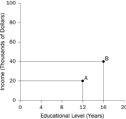
124. The focus is on simple linear regression. See also Rubinfeld, supra note 21, and the Appendix, infra, and Section II, supra, for further discussion of these ideas with an emphasis on econometrics.
125. These data are from a public-use CD, Bureau of the Census, U.S. Department of Commerce, for the March 2005 Current Population Survey. Income and education are self-reported. Income is censored at $100,000. For additional details, see Freedman et al., supra note 12, at A-11. Both variables in a scatter diagram have to be quantitative (with numerical values) rather than qualitative (nonnumerical).
Figure 6 is the scatter diagram for the Kansas data. The diagram confirms an obvious point. There is a positive association between income and education. In general, persons with a higher educational level have higher incomes. However, there are many exceptions to this rule, and the association is not as strong as one might expect.
Figure 6. Scatter diagram for income and education: men ages 25 to 34 in Kansas.
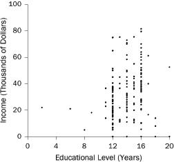
Two variables are positively correlated when their values tend to go up or down together, such as income and education in Figure 5. The correlation coefficient (usually denoted by the letter r) is a single number that reflects the sign of an association and its strength. Figure 7 shows r for three scatter diagrams: In the first, there is no association; in the second, the association is positive and moderate; in the third, the association is positive and strong.
A correlation coefficient of 0 indicates no linear association between the variables. The maximum value for the coefficient is +1, indicating a perfect linear relationship: The dots in the scatter diagram fall on a straight line that slopes up. Sometimes, there is a negative association between two variables: Large values of one tend to go with small values of the other. The age of a car and its fuel economy in miles per gallon illustrate the idea. Negative association is indicated by negative values for r. The extreme case is an r of −1, indicating that all the points in the scatter diagram lie on a straight line that slopes down.
Weak associations are the rule in the social sciences. In Figure 5, the correlation between income and education is about 0.4. The correlation between college grades and first-year law school grades is under 0.3 at most law schools, while the
Figure 7. The correlation coefficient measures the sign of a linear association and its strength.
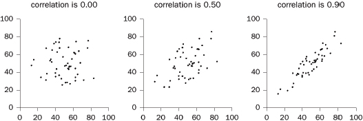
correlation between LSAT scores and first-year grades is generally about 0.4.126 The correlation between heights of fraternal twins is about 0.5. By contrast, the correlation between heights of identical twins is about 0.95.
The correlation coefficient has a number of limitations, to be considered in turn. The correlation coefficient is designed to measure linear association. Figure 8 shows a strong nonlinear pattern with a correlation close to zero. The correlation coefficient is of limited use with nonlinear data.
2. Do outliers influence the correlation coefficient?
The correlation coefficient can be distorted by outliers—a few points that are far removed from the bulk of the data. The left-hand panel in Figure 9 shows that one outlier (lower right-hand corner) can reduce a perfect correlation to nearly nothing. Conversely, the right-hand panel shows that one outlier (upper right-hand corner) can raise a correlation of zero to nearly one. If there are extreme outliers in the data, the correlation coefficient is unlikely to be meaningful.
3. Does a confounding variable influence the coefficient?
The correlation coefficient measures the association between two variables. Researchers—and the courts—are usually more interested in causation. Causation is not the same as association. The association between two variables may be driven by a lurking variable that has been omitted from the analysis (supra
126. Lisa Anthony Stilwell et al., Predictive Validity of the LSAT: A National Summary of the 2001–2002 Correlation Studies 5, 8 (2003).
Figure 8. The scatter diagram shows a strong nonlinear association with a correlation coefficient close to zero. The correlation coefficient only measures the degree of linear association.
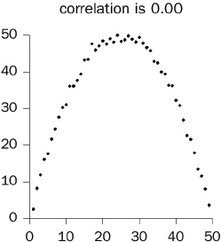
Figure 9. The correlation coefficient can be distorted by outliers.
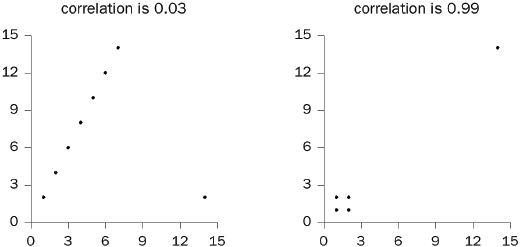
Section II.A). For an easy example, there is an association between shoe size and vocabulary among schoolchildren. However, learning more words does not cause the feet to get bigger, and swollen feet do not make children more articulate. In this case, the lurking variable is easy to spot—age. In more realistic examples, the lurking variable is harder to identify.127
127. Green et al., supra note 13, Section IV.C, provides one such example.
In statistics, lurking variables are called confounders or confounding variables. Association often does reflect causation, but a large correlation coefficient is not enough to warrant causal inference. A large value of r only means that the dependent variable marches in step with the independent one: Possible reasons include causation, confounding, and coincidence. Multiple regression is one method that attempts to deal with confounders (infra Section V.D).128
The regression line can be used to describe a linear trend in the data. The regression line for income on education in the Kansas sample is shown in Figure 10. The height of the line estimates the average income for a given educational level. For example, the average income for people with 8 years of education is estimated at $21,100, indicated by the height of the line at 8 years. The average income for people with 16 years of education is estimated at $34,700.
Figure 10. The regression line for income on education and its estimates.
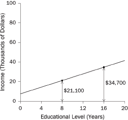
Figure 11 combines the data in Figures 5 and 10: it shows the scatter diagram for income and education, with the regression line superimposed. The line shows the average trend of income as education increases. Thus, the regression line indicates the extent to which a change in one variable (income) is associated with a change in another variable (education).
128. See also Rubinfeld, supra note 21. The difference between experiments and observational studies is discussed supra Section II.B.
Figure 11. Scatter diagram for income and education, with the regression line indicating the trend.
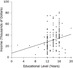
1. What are the slope and intercept?
The regression line can be described in terms of its intercept and slope. Often, the slope is the more interesting statistic. In Figure 11, the slope is $1700 per year. On average, each additional year of education is associated with an additional $1700 of income. Next, the intercept is $7500. This is an estimate of the average income for (hypothetical) persons with zero years of education.129Figure 10 suggests this estimate may not be especially good. In general, estimates based on the regression line become less trustworthy as we move away from the bulk of the data.
The slope of the regression line has the same limitations as the correlation coefficient: (1) The slope may be misleading if the relationship is strongly nonlinear and (2) the slope may be affected by confounders. With respect to (1), the slope of $1700 per year in Figure 10 presents each additional year of education as having the same value, but some years of schooling surely are worth more and
129. The regression line, like any straight line, has an equation of the form y = a + bx. Here, a is the intercept (the value of y when x = 0), and b is the slope (the change in y per unit change in x). In Figure 9, the intercept of the regression line is $7500 and the slope is $1700 per year. The line estimates an average income of $34,700 for people with 16 years of education. This may be computed from the intercept and slope as follows:
$7500 + ($1700 per year) × 16 years = $7500 + $22,200 = $34,700.
The slope b is the same anywhere along the line. Mathematically, that is what distinguishes straight lines from other curves. If the association is negative, the slope will be negative too. The slope is like the grade of a road, and it is negative if the road goes downhill. The intercept is like the starting elevation of a road, and it is computed from the data so that the line goes through the center of the scatter diagram, rather than being generally too high or too low.
others less. With respect to (2), the association between education and income is no doubt causal, but there are other factors to consider, including family background. Compared to individuals who did not graduate from high school, people with college degrees usually come from richer and better educated families. Thus, college graduates have advantages besides education. As statisticians might say, the effects of family background are confounded with the effects of education. Statisticians often use the guarded phrases “on average” and “associated with” when talking about the slope of the regression line. This is because the slope has limited utility when it comes to making causal inferences.
2. What is the unit of analysis?
If association between characteristics of individuals is of interest, these characteristics should be measured on individuals. Sometimes individual-level data are not to be had, but rates or averages for groups are available. “Ecological” correlations are computed from such rates or averages. These correlations generally overstate the strength of an association. For example, average income and average education can be determined for men living in each state and in Washington, D.C. The correlation coefficient for these 51 pairs of averages turns out to be 0.70. However, states do not go to school and do not earn incomes. People do. The correlation for income and education for men in the United States is only 0.42. The correlation for state averages overstates the correlation for individuals—a common tendency for ecological correlations.130
Ecological analysis is often seen in cases claiming dilution in voting strength of minorities. In this type of voting rights case, plaintiffs must prove three things: (1) the minority group constitutes a majority in at least one district of a proposed plan; (2) the minority group is politically cohesive, that is, votes fairly solidly for its preferred candidate; and (3) the majority group votes sufficiently as a bloc to defeat the minority-preferred candidate.131 The first requirement is compactness; the second and third define polarized voting.
130. Correlations are computed from the March 2005 Current Population Survey for men ages 25–64. Freedman et al., supra note 12, at 149. The ecological correlation uses only the average figures, but within each state there is a lot of spread about the average. The ecological correlation smoothes away this individual variation. Cf. Green et al., supra note 13, Section II.B.4 (suggesting that ecological studies of exposure and disease are “far from conclusive” because of the lack of data on confounding variables (a much more general problem) as well as the possible aggregation bias described here); David A. Freedman, Ecological Inference and the Ecological Fallacy, in 6 Int’l Encyclopedia of the Social and Behavioral Sciences 4027 (Neil J. Smelser & Paul B. Baltes eds., 2001).
131. See Thornburg v. Gingles, 478 U.S. 30, 50–51 (1986) (“First, the minority group must be able to demonstrate that it is sufficiently large and geographically compact to constitute a majority in a single-member district…. Second, the minority group must be able to show that it is politically cohesive…. Third, the minority must be able to demonstrate that the white majority votes sufficiently as a bloc to enable it…usually to defeat the minority’s preferred candidate.”). In subsequent cases, the Court has emphasized that these factors are not sufficient to make out a violation of section 2 of
The secrecy of the ballot box means that polarized voting cannot be directly observed. Instead, plaintiffs in voting rights cases rely on ecological regression, with scatter diagrams, correlations, and regression lines to estimate voting behavior by groups and demonstrate polarization. The unit of analysis typically is the precinct. For each precinct, public records can be used to determine the percentage of registrants in each demographic group of interest, as well as the percentage of the total vote for each candidate—by voters from all demographic groups combined. Plaintiffs’ burden is to determine the vote by each demographic group separately.
Figure 12 shows how the argument unfolds. Each point in the scatter diagram represents data for one precinct in the 1982 Democratic primary election for auditor in Lee County, South Carolina. The horizontal axis shows the percentage of registrants who are white. The vertical axis shows the turnout rate for the white candidate. The regression line is plotted too. The slope would be interpreted as the difference between the white turnout rate and the black turnout rate for the white candidate. Furthermore, the intercept would be interpreted as the black turnout rate for the white candidate.132 The validity of such estimates is contested in the statistical literature.133
the Voting Rights Act. E.g., Johnson v. De Grandy, 512 U.S. 997, 1011 (1994) (“Gingles…clearly declined to hold [these factors] sufficient in combination, either in the sense that a court’s examination of relevant circumstances was complete once the three factors were found to exist, or in the sense that the three in combination necessarily and in all circumstances demonstrated dilution.”).
132. By definition, the turnout rate equals the number of votes for the candidate, divided by the number of registrants; the rate is computed separately for each precinct. The intercept of the line in Figure 11 is 4%, and the slope is 0.52. Plaintiffs would conclude that only 4% of the black registrants voted for the white candidate, while 4% + 52% = 56% of the white registrants voted for the white candidate, which demonstrates polarization.
133. For further discussion of ecological regression in this context, see D. James Greiner, Ecological Inference in Voting Rights Act Disputes: Where Are We Now, and Where Do We Want to Be?, 47 Jurimetrics J. 115 (2007); Bernard Grofman & Chandler Davidson, Controversies in Minority Voting: The Voting Rights Act in Perspective (1992); Stephen P. Klein & David A. Freedman, Ecological Regression in Voting Rights Cases, 6 Chance 38 (Summer 1993). The use of ecological regression increased considerably after the Supreme Court noted in Thornburg v. Gingles, 478 U.S. 30, 53 n.20 (1986), that “[t]he District Court found both methods [extreme case analysis and bivariate ecological regression analysis] standard in the literature for the analysis of racially polarized voting.” See, e.g., Cottier v. City of Martin, 445 F.3d 1113, 1118 (8th Cir. 2006) (ecological regression is one of the “proven approaches to evaluating elections”); Bruce M. Clarke & Robert Timothy Reagan, Fed. Judicial Ctr., Redistricting Litigation: An Overview of Legal, Statistical, and Case-Management Issues (2002); Greiner, supra, at 117, 121. Nevertheless, courts have cautioned against “overreliance on bivariate ecological regression” in light of the inherent limitations of the technique. Lewis v. Alamance County, 99 F.3d 600, 604 n.3 (4th Cir. 1996); Johnson v. Hamrick, 296 F.3d 1065, 1080 n.4 (11th Cir. 2002) (“as a general rule, homogenous precinct analysis may be more reliable than ecological regression.”). However, there are problems with both methods. See, e.g., Greiner, supra, at 123–39 (arguing that homogeneous precinct analysis is fundamentally flawed and that courts need to be more discerning in dealing with ecological regression).
Redistricting plans based predominantly on racial considerations are unconstitutional unless narrowly tailored to meet a compelling state interest. Shaw v. Reno, 509 U.S. 630 (1993). Whether compliance with the Voting Rights Act can be considered a compelling interest is an open ques-
Figure 12. Turnout rate for the white candidate plotted against the percentage of registrants who are white. Precinct-level data, 1982 Democratic Primary for Auditor, Lee County, South Carolina.
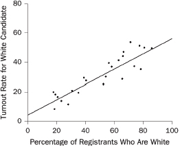
Source: Data from James W. Loewen & Bernard Grofman, Recent Developments in Methods Used in Vote Dilution Litigation, 21 Urb. Law. 589, 591 tbl.1 (1989).
Statistical models are widely used in the social sciences and in litigation. For example, the census suffers an undercount, more severe in certain places than others. If some statistical models are to be believed, the undercount can be corrected—moving seats in Congress and millions of dollars a year in tax funds.134 Other models purport to lift the veil of secrecy from the ballot box, enabling the experts to determine how minority groups have voted—a crucial step in voting rights litigation (supra Section V.C). This section discusses the statistical logic of regression models.
A regression model attempts to combine the values of certain variables (the independent variables) to get expected values for another variable (the dependent variable). The model can be expressed in the form of a regression equation. A simple regression equation has only one independent variable; a multiple regression equation has several independent variables. Coefficients in the equation will be interpreted as showing the effects of changing the corresponding variables. This is justified in some situations, as the next example demonstrates.
tion, but efforts to sustain racially motivated redistricting on this basis have not fared well before the Supreme Court. See Abrams v. Johnson, 521 U.S. 74 (1997); Shaw v. Hunt, 517 U.S. 899 (1996); Bush v. Vera, 517 U.S. 952 (1996).
134. See Brown et al., supra note 29; supra note 89.
Hooke’s law (named after Robert Hooke, England, 1653–1703) describes how a spring stretches in response to a load: Strain is proportional to stress. To verify Hooke’s law experimentally, a physicist will make a number of observations on a spring. For each observation, the physicist hangs a weight on the spring and measures its length. A statistician could develop a regression model for these data:
| length = a + b × weight + e. | (1) |
The error term, denoted by the Greek letter epsilon e, is needed because measured length will not be exactly equal to a + b × weight. If nothing else, measurement error must be reckoned with. The model takes e as “random error”—behaving like draws made at random with replacement from a box of tickets. Each ticket shows a potential error, which will be realized if that ticket is drawn. The average of the potential errors in the box is assumed to be zero.
Equation (1) has two parameters, a and b. These constants of nature characterize the behavior of the spring: a is length under no load, and b is elasticity (the increase in length per unit increase in weight). By way of numerical illustration, suppose a is 400 and b is 0.05. If the weight is 1, the length of the spring is expected to be
400 + 0.05 = 400.05.
If the weight is 3, the expected length is
400 + 3 × 0.05 = 400 + 0.15 = 400.15.
In either case, the actual length will differ from expected, by a random error e.
In standard statistical terminology, the ε’s for different observations on the spring are assumed to be independent and identically distributed, with a mean of zero. Take the ε’s for the first two observations. Independence means that the chances for the second e do not depend on outcomes for the first. If the errors are like draws made at random with replacement from a box of tickets, as we assumed earlier, that box will not change from one draw to the next—independence. “Identically distributed” means that the chance behavior of the two ε’s is the same: They are drawn at random from the same box. (See infra Appendix for additional discussion.)
The parameters a and b in equation (1) are not directly observable, but they can be estimated by the method of least squares.135 Statisticians often denote esti-
135. It might seem that a is observable; after all, we can measure the length of the spring with no load. However, the measurement is subject to error, so we observe not a, but a + e. See equation (1). The parameters a and b can be estimated, even estimated very well, but they cannot be observed directly. The least squares estimates of a and b are the intercept and slope of the regression
mates by hats. Thus, â is the estimate for â, and ![]() is the estimate for b. The values of â and
is the estimate for b. The values of â and ![]() are chosen to minimize the sum of the squared prediction errors. These errors are also called residuals. They measure the difference between the actual length of the spring and the predicted length, the latter being â +
are chosen to minimize the sum of the squared prediction errors. These errors are also called residuals. They measure the difference between the actual length of the spring and the predicted length, the latter being â + ![]() × weight:
× weight:
| actual length = â + |
(2) |
Of course, no one really imagines there to be a box of tickets hidden in the spring. However, the variability of physical measurements (under many but by no means all circumstances) does seem to be remarkably like the variability in draws from a box.136 In short, the statistical model corresponds rather closely to the empirical phenomenon.
Equation (1) is a statistical model for the data, with unknown parameters a and b. The error term e is not observable. The model is a theory—and a good one—about how the data are generated. By contrast, equation (2) is a regression equation that is fitted to the data: The intercept â, the slope ![]() , and the residual can all be computed from the data. The results are useful because â is a good estimate for a, and
, and the residual can all be computed from the data. The results are useful because â is a good estimate for a, and ![]() is a good estimate for b. (Similarly, the residual is a good approximation to e.) Without the theory, these estimates would be less useful. Is there a theoretical model behind the data processing? Is the model justifiable? These questions can be critical when it comes to making statistical inferences from the data.
is a good estimate for b. (Similarly, the residual is a good approximation to e.) Without the theory, these estimates would be less useful. Is there a theoretical model behind the data processing? Is the model justifiable? These questions can be critical when it comes to making statistical inferences from the data.
In social science applications, statistical models often are invoked without an independent theoretical basis. We give an example involving salary discrimination in the Appendix.137 The main ideas of such regression modeling can be captured in a hypothetical exchange between a plaintiff seeking to prove salary discrimination and a company denying the allegation. Such a dialog might proceed as follows:
- Plaintiff argues that the defendant company pays male employees more than females, which establishes a prima facie case of discrimination.
- The company responds that the men are paid more because they are better educated and have more experience.
- Plaintiff refutes the company’s theory by fitting a regression equation that includes a particular, presupposed relationship between salary (the dependent variable) and some measures of education and experience. Plaintiff’s expert reports that even after adjusting for differences in education and
line. See supra Section V.C.1; Freedman et al., supra note 12, at 208–10. The method of least squares was developed by Adrien-Marie Legendre (France, 1752–1833) and Carl Friedrich Gauss (Germany, 1777–1855) to fit astronomical orbits.
136. This is the Gauss model for measurement error. See Freedman et al., supra note 12, at 450–52.
137. The Reference Guide to Multiple Regression in this manual describes a comparable example.
-
in this specific manner, men earn more than women. This remaining difference in pay shows discrimination.
- The company argues that the difference could be the result of chance, not discrimination.
- Plaintiff replies that because the coefficient for gender in the model is statistically significant, chance is not a good explanation for the data.138
In step 3, the three explanatory variables are education (years of schooling completed), experience (years with the firm), and a dummy variable for gender (1 for men and 0 for women). These are supposed to predict salaries (dollars per year). The equation is a formal analog of Hooke’s law (equation 1). According to the model, an employee’s salary is determined as if by computing
| a + (b × education) + (c × experience) + (d × gender), | (3) |
and then adding an error e drawn at random from a box of tickets.139 The parameters a, b, c, and d, are estimated from the data by the method of least squares.
In step 5, the estimated coefficient d for the dummy variable turns out to be positive and statistically significant and is offered as evidence of disparate impact. Men earn more than women, even after adjusting for differences in background factors that might affect productivity. This showing depends on many assumptions built into the model.140 Hooke’s law—equation (1)—is relatively easy to test experimentally. For the salary discrimination model, validation would be difficult. When expert testimony relies on statistical models, the court may well inquire, what are the assumptions behind the model, and why do they apply to the case at hand? It might then be important to distinguish between two situations:
- The nature of the relationship between the variables is known and regression is being used to make quantitative estimates of parameters in that relationship, or
- The nature of the relationship is largely unknown and regression is being used to determine the nature of the relationship—or indeed whether any relationship exists at all.
138. In some cases, the p-value has been interpreted as the probability that defendants are innocent of discrimination. However, as noted earlier, such an interpretation is wrong: p merely represents the probability of getting a large test statistic, given that the model is correct and the true coefficient for gender is zero (see supra Section IV.B, infra Appendix, Section D.2). Therefore, even if we grant the model, a p-value less than 50% does not demonstrate a preponderance of the evidence against the null hypothesis.
139. Expression (3) is the expected value for salary, given the explanatory variables (education, experience, gender). The error term is needed to account for deviations from expected: Salaries are not going to be predicted very well by linear combinations of variables such as education and experience.
140. See infra Appendix.
Regression was developed to handle situations of the first type, with Hooke’s law being an example. The basis for the second type of application is analogical, and the tightness of the analogy is an issue worth exploration.
In employment discrimination cases, and other contexts too, a wide variety of models can be used. This is only to be expected, because the science does not dictate specific equations. In a strongly contested case, each side will have its own model, presented by its own expert. The experts will reach opposite conclusions about discrimination. The dialog might continue with an exchange about which model is better. Although statistical assumptions are challenged in court from time to time, arguments more commonly revolve around the choice of variables. One model may be questioned because it omits variables that should be included—for example, skill levels or prior evaluations.141 Another model may be challenged because it includes tainted variables reflecting past discriminatory behavior by the firm.142 The court must decide which model—if either—fits the occasion.143
The frequency with which regression models are used is no guarantee that they are the best choice for any particular problem. Indeed, from one perspective, a regression or other statistical model may seem to be a marvel of mathematical rigor. From another perspective, the model is a set of assumptions, supported only by the say-so of the testifying expert. Intermediate judgments are also possible.144
141. E.g., Bazemore v. Friday, 478 U.S. 385 (1986); In re Linerboard Antitrust Litig., 497 F. Supp. 2d 666 (E.D. Pa. 2007).
142. E.g., McLaurin v. Nat’l R.R. Passenger Corp., 311 F. Supp. 2d 61, 65–66 (D.D.C. 2004) (holding that the inclusion of two allegedly tainted variables was reasonable in light of an earlier consent decree).
143. E.g., Chang v. Univ. of R.I., 606 F. Supp. 1161, 1207 (D.R.I. 1985) (“it is plain to the court that [defendant’s] model comprises a better, more useful, more reliable tool than [plaintiff’s] counterpart.”); Presseisen v. Swarthmore College, 442 F. Supp. 593, 619 (E.D. Pa. 1977) (“[E]ach side has done a superior job in challenging the other’s regression analysis, but only a mediocre job in supporting their own…and the Court is…left with nothing.”), aff’d, 582 F.2d 1275 (3d Cir. 1978).
144. See, e.g., David W. Peterson, Reference Guide on Multiple Regression, 36 Jurimetrics J. 213, 214–15 (1996) (review essay); see supra note 21 for references to a range of academic opinion. More recently, some investigators have turned to graphical models. However, these models have serious weaknesses of their own. See, e.g., David A. Freedman, On Specifying Graphical Models for Causation, and the Identification Problem, 26 Evaluation Rev. 267 (2004).
The mathematical theory of probability consists of theorems derived from axioms and definitions. Mathematical reasoning is seldom controversial, but there may be disagreement as to how the theory should be applied. For example, statisticians may differ on the interpretation of data in specific applications. Moreover, there are two main schools of thought about the foundations of statistics: frequentist and Bayesian (also called objectivist and subjectivist).145
Frequentists see probabilities as empirical facts. When a fair coin is tossed, the probability of heads is 1/2; if the experiment is repeated a large number of times, the coin will land heads about one-half the time. If a fair die is rolled, the probability of getting an ace (one spot) is 1/6. If the die is rolled many times, an ace will turn up about one-sixth of the time.146 Generally, if a chance experiment can be repeated, the relative frequency of an event approaches (in the long run) its probability. By contrast, a Bayesian considers probabilities as representing not facts but degrees of belief: In whole or in part, probabilities are subjective.
Statisticians of both schools use conditional probability—that is, the probability of one event given that another has occurred. For example, suppose a coin is tossed twice. One event is that the coin will land HH. Another event is that at least one H will be seen. Before the coin is tossed, there are four possible, equally likely, outcomes: HH, HT, TH, TT. So the probability of HH is 1/4. However, if we know that at least one head has been obtained, then we can rule out two tails TT. In other words, given that at least one H has been obtained, the conditional probability of TT is 0, and the first three outcomes have conditional probability 1/3 each. In particular, the conditional probability of HH is 1/3. This is usually written as P(HH|at least one H) = 1/3. More generally, the probability of an event C is denoted P(C); the conditional probability of D given C is written as P(D|C).
Two events C and D are independent if the conditional probability of D given that C occurs is equal to the conditional probability of D given that C does not occur. Statisticians use “~C” to denote the event that C does not occur. Thus C and D are independent if P(D|C) = P(D|~C). If C and D are independent, then the probability that both occur is equal to the product of the probabilities:
| P(C and D) = P(C) × P(D). | (A1) |
145. But see supra note 123 (on “objective Bayesianism”).
146. Probabilities may be estimated from relative frequencies, but probability itself is a subtler idea. For example, suppose a computer prints out a sequence of 10 letters H and T (for heads and tails), which alternate between the two possibilities H and T as follows: H T H T H T H T H T. The relative frequency of heads is 5/10 or 50%, but it is not at all obvious that the chance of an H at the next position is 50%. There are difficulties in both the subjectivist and objectivist positions. See Freedman, supra note 84.
This is the multiplication rule (or product rule) for independent events. If events are dependent, then conditional probabilities must be used:
| P(C and D) = P(C) × P(D|C). | (A2) |
This is the multiplication rule for dependent events.
Bayesian statisticians assign probabilities to hypotheses as well as to events; indeed, for them, the distinction between hypotheses and events may not be a sharp one. We turn now to Bayes’ rule. If H0 and H1 are two hypotheses147 that govern the probability of an event A, a Bayesian can use the multiplication rule (A2) to find that
| P(A and H0) = P(A|H0)P(H0) | (A3) |
and
| P(A and H1) = P(A|H1)P(H1). | (A4) |
Moreover,
| P(A) = P(A and H0) + P(A and H1). | (A5) |
The multiplication rule (A2) also shows that
| (A6) |
We use (A4) to evaluate P(A and H1) in the numerator of (A6), and (A3), (A4), and (A5) to evaluate P(A) in the denominator:
| (A7) |
This is a special case of Bayes’ rule. It yields the conditional probability of hypothesis H0 given that event A has occurred.
For a stylized example in a criminal case, H0 is the hypothesis that blood found at the scene of a crime came from a person other than the defendant; H1 is the hypothesis that the blood came from the defendant; A is the event that blood from the crime scene and blood from the defendant are both type A. Then P(H0) is the prior probability of H0, based on subjective judgment, while P(H0|A) is the posterior probability—updated from the prior using the data.
147. H 0 is read “H-sub-zero,” while H1 is “H-sub-one.”
Type A blood occurs in 42% of the population. So P(A|H0) = 0.42.148 Because the defendant has type A blood, P(A|H1) = 1. Suppose the prior probabilities are P(H0) = P(H1) = 0.5. According to (A7), the posterior probability that the blood is from the defendant is
| (A8) |
Thus, the data increase the likelihood that the blood is the defendant’s. The probability went up from the prior value of P(H1) = 0.50 to the posterior value of P(H1|A) = 0.70.
More generally, H0 and H1 refer to parameters in a statistical model. For a stylized example in an employment discrimination case, H0 asserts equal selection rates in a population of male and female applicants; H1 asserts that the selection rates are not equal; A is the event that a test statistic exceeds 2 in absolute value. In such situations, the Bayesian proceeds much as before. However, the frequentist computes P(A|H0), and rejects H0 if this probability falls below 5%. Frequentists have to stop there, because they view P(H0|A) as poorly defined at best. In their setup, P(H0) and P(H1) rarely make sense, and these prior probabilities are needed to compute P(H1|A): See supra equation (A7).
Assessing probabilities, conditional probabilities, and independence is not entirely straightforward, either for frequentists or Bayesians. Inquiry into the basis for expert judgment may be useful, and casual assumptions about independence should be questioned.149
B. The Spock Jury: Technical Details
The rest of this Appendix provides some technical backup for the examples in Sections IV and V, supra. We begin with the Spock jury case. On the null hypothesis, a sample of 350 people was drawn at random from a large population that was 50% male and 50% female. The number of women in the sample follows the binomial distribution. For example, the chance of getting exactly 102 women in the sample is given by the binomial formula150
| (A9) |
148. Not all statisticians would accept the identification of a population frequency with P(A|H 0). Indeed, H0 has been translated into a hypothesis that the true donor has been selected from the population at random (i.e., in a manner that is uncorrelated with blood type). This step needs justification. See supra note 123.
149. For problematic assumptions of independence in litigation, see, e.g., Wilson v. State, 803 A.2d 1034 (Md. 2002) (error to admit multiplied probabilities in a case involving two deaths of infants in same family); 1 McCormick, supra note 2, § 210; see also supra note 29 (on census litigation).
150. The binomial formula is discussed in, e.g., Freedman et al., supra note 12, at 255–61.
In the formula, n stands for the sample size, and so n = 350; and j = 102. The f is the fraction of women in the population; thus, f = 0.50. The exclamation point denotes factorials: 1! = 1, 2! = 2 × 1 = 2, 3! = 3 × 2 × 1 = 6, and so forth. The chance of 102 women works out to 10–15. In the same way, we can compute the chance of getting 101 women, or 100, or any other particular number. The chance of getting 102 women or fewer is then computed by addition. The chance is p = 2 × 10–15, as reported supra note 98. This is very bad news for the null hypothesis.
With the binomial distribution given by (9), the expected the number of women in the sample is
| n f = 350 × 05 . = 175. | (A10) |
The standard error is
| (A11) |
The observed value of 102 is nearly 8 SEs below the expected value, which is a lot of SEs.
Figure 13 shows the probability histogram for the number of women in the sample.151 The graph is drawn so that the area between two values is proportional to the chance that the number of women will fall in that range. For example, take the rectangle over 175; its base covers the interval from 174.5 to 175.5. The area of this rectangle is 4.26% of the total area. So the chance of getting exactly 175 women is 4.26%. Next, take the range from 165 to 185 (inclusive): 73.84% of the area falls into this range. This means there is a 73.84% chance that the number of women in the sample will be in the range from 165 to 185 (inclusive).
According to a fundamental theorem in statistics (the central limit theorem), the histogram follows the normal curve.152Figure 13 shows the curve for comparison: The normal curve is almost indistinguishable from the top of the histogram. For a numerical example, suppose the jury panel had included 155 women. On the null hypothesis, there is about a 1.85% chance of getting 155 women or fewer. The normal curve gives 1.86%. The error is nil. Ordinarily, we would just report p = 2%, as in the text (supra Section IV.B.1).
Finally, we consider power. Suppose we reject the null hypothesis when the number of women in the sample is 155 or less. Let us assume a particular alternative hypothesis that quantifies the degree of discrimination against women: The jury panel is selected at random from a population that is 40% female, rather than 50%. Figure 14 shows the probability histogram for the number of women, but now the histogram is computed according to the alternative hypothesis. Again,
151. Probability histograms are discussed in, e.g., id. at 310–13.
152. The central limit theorem is discussed in, e.g., id. at 315–27.
Figure 13. Probability histogram for the number of women in a random sample of 350 people drawn from a large population that is 50% female and 50% male. The normal curve is shown for comparison. About 2% of the area under the histogram is to the left of 155 (marked by a heavy vertical line).
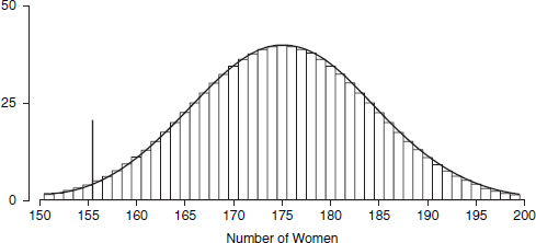
Note: The vertical line is placed at 155.5, and so the area to the left of it includes the rectangles over 155, 154,…; the area represents the chance of getting 155 women or fewer. Cf. Freedman et al., supra note 12, at 317. The units on the vertical axis are “percent per standard unit”; cf. id. at 80, 315.
Figure 14. Probability histogram for the number of women in a random sample of 350 people drawn from a large population that is 40% female and 60% male. The normal curve is shown for comparison. The area to the left of 155 (marked by a heavy vertical line) is about 95%.
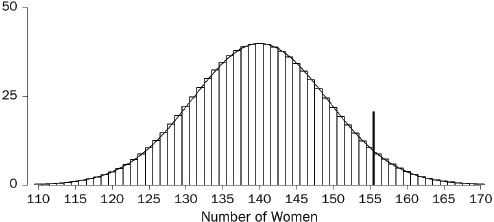
the histogram follows the normal curve. About 95% of the area is to the left of 155, and so power is about 95%. The area can be computed exactly by using the binomial distribution, or to an excellent approximation using the normal curve.
Figures 13 and 14 have the same shape: The central limit theorem is at work. However, the histograms are centered differently. Figure 13 is centered at 175, according to requirements of the null hypothesis. Figure 14 is centered at 140, because the alternative hypothesis is used to determine the center, not the null hypothesis. Thus, 155 is well to the left of center in Figure 13, and well to the right in Figure 14: The figures have different centers. The main point of Figures 13 and 14 is that chances can often be approximated by areas under the normal curve, justifying the large-sample theory presented supra Sections IV.A–B.
C. The Nixon Papers: Technical Details
With the Nixon papers, the population consists of 20,000 boxes. A random sample of 500 boxes is drawn and each sample box is appraised. Statistical theory enables us to make some precise statements about the behavior of the sample average.
- The expected value of the sample average equals the population average. Even more tersely, the sample average is an unbiased estimate of the population average.
- The standard error for the sample average equals
| (A12) |
In (A12), the N stands for the size of the population, which is 20,000; and n stands for the size of the sample, which is 500. The first factor in (A12), with the square root, is the finite sample correction factor. Here, as in many other such examples, the correction factor is so close to 1 that it can safely be ignored. (This is why the size of population usually has no bearing on the precision of the sample average as an estimator for the population average.) Next, σ is the population standard deviation. This is unknown, but it can be estimated by the sample standard deviation, which is $2200. The SE for the sample mean is therefore estimated from the data as $2200/![]() , which is nearly $100. Plaintiff’s total claim is 20,000 times the sample average. The SE for the total claim is therefore 20,000 × $100 = $2,000,000. (Here, the size of the population comes into the formula.)
, which is nearly $100. Plaintiff’s total claim is 20,000 times the sample average. The SE for the total claim is therefore 20,000 × $100 = $2,000,000. (Here, the size of the population comes into the formula.)
With a large sample, the probability histogram for the sample average follows the normal curve quite closely. That is a consequence of the central limit theorem. The center of the histogram is the population average. The SE is given by (A12), and is about $100.
- What is the chance that the sample average differs from the population average by 1 SE or less? This chance is equal to the area under the probability histogram within 1 SE of average, which by the central limit theorem is almost equal to the area under the standard normal curve between −1 and 1; that normal area is about 68%.
- What is the chance that the sample average differs from the population average by 2 SE or less? By the same reasoning, this chance is about equal to the area under the standard normal curve between −2 and 2, which is about 95%.
- What is the chance that the sample average differs from the population average by 3 SE or less? This chance is about equal to the area under the standard normal curve between −3 and 3, which is about 99.7%.
To sum up, the probability histogram for the sample average is centered at the population average. The spread is given by the standard error. The histogram follows the normal curve. That is why confidence levels can be based on the standard error, with confidence levels read off the normal curve—for estimators that are essentially unbiased, and obey the central limit theorem (supra Section IV.A.2, Appendix Section B).153 These large-sample methods generally work for sums, averages, and rates, although much depends on the design of the sample.
More technically, the normal curve is the density of a normal distribution. The standard normal density has mean equal to 0 and standard error equal to 1. Its equation is
![]()
where e = 2.71828…and p = 3.14159…. This density can be rescaled to have any desired mean and standard error. The resulting densities are the famous “normal curves” or “bell-shaped curves” of statistical theory. In Figure 12, the density is scaled to match the probability histogram in terms of the mean and standard error; likewise in Figure 13.
D. A Social Science Example of Regression: Gender Discrimination in Salaries
To illustrate social science applications of the kind that might be seen in litigation, Section V referred to a stylized example on salary discrimination. A particular
153. See, e.g., id. at 409–24. On the standard deviation, see supra Section III.E; Freedman et al., supra note 12, at 67–72. The finite sample correction factor is discussed in id. at 367–70.
regression model was used to predict salaries (dollars per year) of employees in a firm. It had three explanatory variables: education (years of schooling completed), experience (years with the firm), and a dummy variable for gender (1 for men and 0 for women). The regression equation is
| salary = a + b × education + c × experience + d × gender + e. | (A13) |
Equation (A13) is a statistical model for the data, with unknown parameters a, b, c, and d. Here, a is the intercept and the other parameters are regression coefficients. The e at the end of the equation is an unobservable error term. In the right-hand side of (A3) and similar expressions, by convention, the multiplications are done before the additions.
As noted in Section V, the equation is a formal analog of Hooke’s law (1). According to the model, an employee’s salary is determined as if by computing
| a + b × education + c × experience + d × gender | (A14) |
and then adding an error e drawn at random from a box of tickets. Expression (A14) is the expected value for salary, given the explanatory variables (education, experience, gender). The error term is needed to account for deviations from expected: Salaries are not going to be predicted very well by linear combinations of variables such as education and experience.
The parameters are estimated from the data using least squares. If the estimated coefficient for the dummy variable turns out to be positive and statistically significant, that would be evidence of disparate impact. Men earn more than women, even after adjusting for differences in background factors that might affect productivity. Suppose the estimated equation turns out as follows:
| predicted salary = $7100 + $1300 × education + $2200 × experience + $700 × gender. |
(A15) |
According to (A15), the estimated value for the intercept a in (A14) is $7100; the estimated value for the coefficient b is $1300, and so forth. According to equation (A15), every extra year of education is worth $1300. Similarly, every extra year of experience is worth $2200. And, most important, the company gives men a salary premium of $700 over women with the same education and experience.
A male employee with 12 years of education (high school) and 10 years of experience, for example, would have a predicted salary of
| $7100 + $1300 × 12 + $2200 × 10 + $700 × 1 = $7100 + $15,600 + $22,000 + $700 = $45,400. |
(A16) |
A similarly situated female employee has a predicted salary of only
| $7100 + $1300 × 12 + $2200 × 10 + $700 × 0 = $7100 + $15,600 + $22,000 + $0 = $44,700. |
(A17) |
Notice the impact of the gender variable in the model: $700 is added to equation (A16), but not to equation (A17).
A major step in proving discrimination is showing that the estimated coefficient of the gender variable—$700 in the numerical illustration—is statistically significant. This showing depends on the assumptions built into the model. Thus, each extra year of education is assumed to be worth the same across all levels of experience. Similarly, each extra year of experience is worth the same across all levels of education. Furthermore, the premium paid to men does not depend systematically on education or experience. Omitted variables such as ability, quality of education, or quality of experience do not make any systematic difference to the predictions of the model.154 These are all assumptions made going into the analysis, rather than conclusions coming out of the data.
Assumptions are also made about the error term—the mysterious e at the end of (A13). The errors are assumed to be independent and identically distributed from person to person in the dataset. Such assumptions are critical when computing p-values and demonstrating statistical significance. Regression modeling that does not produce statistically significant coefficients will not be good evidence of discrimination, and statistical significance cannot be established unless stylized assumptions are made about unobservable error terms.
The typical regression model, like the one sketched above, therefore involves a host of assumptions. As noted in Section V, Hooke’s law—equation (1)—is relatively easy to test experimentally. For the salary discrimination model—equation (A13)—validation would be difficult. That is why we suggested that when expert testimony relies on statistical models, the court may well inquire about the assumptions behind the model and why they apply to the case at hand.
2. Standard errors, t-statistics, and statistical significance
Statistical proof of discrimination depends on the significance of the estimated coefficient for the gender variable. Significance is determined by the t-test, using the standard error. The standard error measures the likely difference between the estimated value for the coefficient and its true value. The estimated value is $700—the coefficient of the gender variable in equation (A5); the true value d in (A13), remains unknown. According to the model, the difference between the estimated value and the true value is due to the action of the error term e in (A3). Without e, observed values would line up perfectly with expected values,
154. Technically, these omitted variables are assumed to be independent of the error term in the equation.
and estimated values for parameters would be exactly equal to true values. This does not happen.
The t-statistic is the estimated value divided by its standard error. For example, in (A15), the estimate for d is $700. If the standard error is $325, then t is $700/$325 = 2.15. This is significant—that is, hard to explain as the product of random error. Under the null hypothesis that d is zero, there is only about a 5% chance that the absolute value of t is greater than 2. (We are assuming the sample is large.) Thus, statistical significance is achieved (supra Section IV.B.2). Significance would be taken as evidence that d—the true parameter in the model (A13)—does not vanish. According to a viewpoint often presented in the social science journals and the courtroom, here is statistical proof that gender matters in determining salaries. On the other hand, if the standard error is $1400, then t is $700/$1400 = 0.5. The difference between the estimated value of d and zero could easily result from chance. So the true value of d could well be zero, in which case gender does not affect salaries.
Of course, the parameter d is only a construct in a model. If the model is wrong, the standard error, t-statistic, and significance level are rather difficult to interpret. Even if the model is granted, there is a further issue. The 5% is the chance that the absolute value of t exceeds 2, given the model and given the null hypothesis that d is zero. However, the 5% is often taken to be the chance of the null hypothesis given the data. This misinterpretation is commonplace in the social science literature, and it appears in some opinions describing expert testimony.155 For a frequentist statistician, the chance that d is zero given the data makes no sense: Parameters do not exhibit chance variation. For a Bayesian statistician, the chance that d is zero given the data makes good sense, but the computation via the t-test could be seriously in error, because the prior probability that d is zero has not been taken into account.156
The mathematical terminology in the previous paragraph may need to be deciphered: The “absolute value” of t is the magnitude, ignoring sign. Thus, the absolute value of both +3 and −3 is 3.
155. See supra Section IV.B & notes 102 & 116.
156. See supra Section IV & supra Appendix.
The following definitions are adapted from a variety of sources, including Michael O. Finkelstein & Bruce Levin, Statistics for Lawyers (2d ed. 2001), and David A. Freedman et al., Statistics (4th ed. 2007).
absolute value. Size, neglecting sign. The absolute value of +2.7 is 2.7; so is the absolute value of -2.7.
adjust for. See control for.
alpha (a). A symbol often used to denote the probability of a Type I error. See Type I error; size. Compare beta.
alternative hypothesis. A statistical hypothesis that is contrasted with the null hypothesis in a significance test. See statistical hypothesis; significance test.
area sample. A probability sample in which the sampling frame is a list of geographical areas. That is, the researchers make a list of areas, choose some at random, and interview people in the selected areas. This is a cost-effective way to draw a sample of people. See probability sample; sampling frame.
arithmetic mean. See mean.
average. See mean.
Bayes’ rule. In its simplest form, an equation involving conditional probabilities that relates a “prior probability” known or estimated before collecting certain data to a “posterior probability” that reflects the impact of the data on the prior probability. In Bayesian statistical inference, “the prior” expresses degrees of belief about various hypotheses. Data are collected according to some statistical model; at least, the model represents the investigator’s beliefs. Bayes’ rule combines the prior with the data to yield the posterior probability, which expresses the investigator’s beliefs about the parameters, given the data. See Appendix A. Compare frequentist.
beta (β). A symbol sometimes used to denote power, and sometimes to denote the probability of a Type II error. See Type II error; power. Compare alpha.
between-observer variability. Differences that occur when two observers measure the same thing. Compare within-observer variability.
bias. Also called systematic error. A systematic tendency for an estimate to be too high or too low. An estimate is unbiased if the bias is zero. (Bias does not mean prejudice, partiality, or discriminatory intent.) See nonsampling error. Compare sampling error.
bin. A class interval in a histogram. See class interval; histogram.
binary variable. A variable that has only two possible values (e.g., gender). Called a dummy variable when the two possible values are 0 and 1.
binomial distribution. A distribution for the number of occurrences in repeated, independent “trials” where the probabilities are fixed. For example, the num-
ber of heads in 100 tosses of a coin follows a binomial distribution. When the probability is not too close to 0 or 1 and the number of trials is large, the binomial distribution has about the same shape as the normal distribution. See normal distribution; Poisson distribution.
blind. See double-blind experiment.
bootstrap. Also called resampling; Monte Carlo method. A procedure for estimating sampling error by constructing a simulated population on the basis of the sample, then repeatedly drawing samples from the simulated population.
categorical data; categorical variable. See qualitative variable. Compare quantitative variable.
central limit theorem. Shows that under suitable conditions, the probability histogram for a sum (or average or rate) will follow the normal curve. See histogram; normal curve.
chance error. See random error; sampling error.
chi-squared (c2). The chi-squared statistic measures the distance between the data and expected values computed from a statistical model. If the chi-squared statistic is too large to explain by chance, the data contradict the model. The definition of “large” depends on the context. See statistical hypothesis; significance test.
class interval. Also, bin. The base of a rectangle in a histogram; the area of the rectangle shows the percentage of observations in the class interval. See histogram.
cluster sample. A type of random sample. For example, investigators might take households at random, then interview all people in the selected households. This is a cluster sample of people: A cluster consists of all the people in a selected household. Generally, clustering reduces the cost of interviewing. See multistage cluster sample.
coefficient of determination. A statistic (more commonly known as R-squared) that describes how well a regression equation fits the data. See R-squared.
coefficient of variation. A statistic that measures spread relative to the mean: SD/mean, or SE/expected value. See expected value; mean; standard deviation; standard error.
collinearity. See multicollinearity.
conditional probability. The probability that one event will occur given that another has occurred.
confidence coefficient. See confidence interval.
confidence interval. An estimate, expressed as a range, for a parameter. For estimates such as averages or rates computed from large samples, a 95% confidence interval is the range from about two standard errors below to two standard errors above the estimate. Intervals obtained this way cover the true
value about 95% of the time, and 95% is the confidence level or the confidence coefficient. See central limit theorem; standard error.
confidence level. See confidence interval.
confounding variable; confounder. A confounder is correlated with the independent variable and the dependent variable. An association between the dependent and independent variables in an observational study may not be causal, but may instead be due to confounding. See controlled experiment; observational study.
consistent estimator. An estimator that tends to become more and more accurate as the sample size grows. Inconsistent estimators, which do not become more accurate as the sample gets larger, are frowned upon by statisticians.
content validity. The extent to which a skills test is appropriate to its intended purpose, as evidenced by a set of questions that adequately reflect the domain being tested. See validity. Compare reliability.
continuous variable. A variable that has arbitrarily fine gradations, such as a person’s height. Compare discrete variable.
control for. Statisticians may control for the effects of confounding variables in nonexperimental data by making comparisons for smaller and more homogeneous groups of subjects, or by entering the confounders as explanatory variables in a regression model. To “adjust for” is perhaps a better phrase in the regression context, because in an observational study the confounding factors are not under experimental control; statistical adjustments are an imperfect substitute. See regression model.
control group. See controlled experiment.
controlled experiment. An experiment in which the investigators determine which subjects are put into the treatment group and which are put into the control group. Subjects in the treatment group are exposed by the investigators to some influence—the treatment; those in the control group are not so exposed. For example, in an experiment to evaluate a new drug, subjects in the treatment group are given the drug, and subjects in the control group are given some other therapy; the outcomes in the two groups are compared to see whether the new drug works.
Randomization—that is, randomly assigning subjects to each group—is usually the best way to ensure that any observed difference between the two groups comes from the treatment rather than from preexisting differences. Of course, in many situations, a randomized controlled experiment is impractical, and investigators must then rely on observational studies. Compare observational study.
convenience sample. A nonrandom sample of units, also called a grab sample. Such samples are easy to take but may suffer from serious bias. Typically, mall samples are convenience samples.
correlation coefficient. A number between −1 and 1 that indicates the extent of the linear association between two variables. Often, the correlation coefficient is abbreviated as r.
covariance. A quantity that describes the statistical interrelationship of two variables. Compare correlation coefficient; standard error; variance.
covariate. A variable that is related to other variables of primary interest in a study; a measured confounder; a statistical control in a regression equation.
criterion. The variable against which an examination or other selection procedure is validated. See validity.
data. Observations or measurements, usually of units in a sample taken from a larger population.
degrees of freedom. See t-test.
dependence. Two events are dependent when the probability of one is affected by the occurrence or non-occurrence of the other. Compare independence; dependent variable.
dependent variable. Also called outcome variable. Compare independent variable.
descriptive statistics. Like the mean or standard deviation, used to summarize data.
differential validity. Differences in validity across different groups of subjects. See validity.
discrete variable. A variable that has only a small number of possible values, such as the number of automobiles owned by a household. Compare continuous variable.
distribution. See frequency distribution; probability distribution; sampling distribution.
disturbance term. A synonym for error term.
double-blind experiment. An experiment with human subjects in which neither the diagnosticians nor the subjects know who is in the treatment group or the control group. This is accomplished by giving a placebo treatment to patients in the control group. In a single-blind experiment, the patients do not know whether they are in treatment or control; the diagnosticians have this information.
dummy variable. Generally, a dummy variable takes only the values 0 or 1, and distinguishes one group of interest from another. See binary variable; regression model.
econometrics. Statistical study of economic issues.
epidemiology. Statistical study of disease or injury in human populations.
error term. The part of a statistical model that describes random error, i.e., the impact of chance factors unrelated to variables in the model. In econometrics, the error term is called a disturbance term.
estimator. A sample statistic used to estimate the value of a population parameter. For example, the sample average commonly is used to estimate the population average. The term “estimator” connotes a statistical procedure, whereas an “estimate” connotes a particular numerical result.
expected value. See random variable.
experiment. See controlled experiment; randomized controlled experiment. Compare observational study.
explanatory variable. See independent variable; regression model.
external validity. See validity.
factors. See independent variable.
Fisher’s exact test. A statistical test for comparing two sample proportions. For example, take the proportions of white and black employees getting a promotion. An investigator may wish to test the null hypothesis that promotion does not depend on race. Fisher’s exact test is one way to arrive at a p-value. The calculation is based on the hypergeometric distribution. For details, see Michael O. Finkelstein and Bruce Levin, Statistics for Lawyers 154–56 (2d ed. 2001). See hypergeometric distribution; p-value; significance test; statistical hypothesis.
fitted value. See residual.
fixed significance level. Also alpha; size. A preset level, such as 5% or 1%; if the p-value of a test falls below this level, the result is deemed statistically significant. See significance test. Compare observed significance level; p-value.
frequency; relative frequency. Frequency is the number of times that something occurs; relative frequency is the number of occurrences, relative to a total. For example, if a coin is tossed 1000 times and lands heads 517 times, the frequency of heads is 517; the relative frequency is 0.517, or 51.7%.
frequency distribution. Shows how often specified values occur in a dataset.
frequentist. Also called objectivist. Describes statisticians who view probabilities as objective properties of a system that can be measured or estimated. Compare Bayesian. See Appendix.
Gaussian distribution. A synonym for the normal distribution. See normal distribution.
general linear model. Expresses the dependent variable as a linear combination of the independent variables plus an error term whose components may be dependent and have differing variances. See error term; linear combination; variance. Compare regression model.
grab sample. See convenience sample.
heteroscedastic. See scatter diagram.
highly significant. See p-value; practical significance; significance test.
histogram. A plot showing how observed values fall within specified intervals, called bins or class intervals. Generally, matters are arranged so that the area under the histogram, but over a class interval, gives the frequency or relative frequency of data in that interval. With a probability histogram, the area gives the chance of observing a value that falls in the corresponding interval.
homoscedastic. See scatter diagram.
hypergeometric distribution. Suppose a sample is drawn at random, without replacement, from a finite population. How many times will items of a certain type come into the sample? The hypergeometric distribution gives the probabilities. For more details, see 1 William Feller, An Introduction to Probability Theory and Its Applications 41–42 (2d ed. 1957). Compare Fisher’s exact test.
hypothesis. See alternative hypothesis; null hypothesis; one-sided hypothesis; significance test; statistical hypothesis; two-sided hypothesis.
hypothesis test. See significance test.
identically distributed. Random variables are identically distributed when they have the same probability distribution. For example, consider a box of numbered tickets. Draw tickets at random with replacement from the box. The draws will be independent and identically distributed.
independence. Also, statistical independence. Events are independent when the probability of one is unaffected by the occurrence or non-occurrence of the other. Compare conditional probability; dependence; independent variable; dependent variable.
independent variable. Independent variables (also called explanatory variables, predictors, or risk factors) represent the causes and potential confounders in a statistical study of causation; the dependent variable represents the effect. In an observational study, independent variables may be used to divide the population up into smaller and more homogenous groups (“stratification”). In a regression model, the independent variables are used to predict the dependent variable. For example, the unemployment rate has been used as the independent variable in a model for predicting the crime rate; the unemployment rate is the independent variable in this model, and the crime rate is the dependent variable. The distinction between independent and dependent variables is unrelated to statistical independence. See regression model. Compare dependent variable; dependence; independence.
indicator variable. See dummy variable.
internal validity. See validity.
interquartile range. Difference between 25th and 75th percentile. See percentile.
interval estimate. A confidence interval, or an estimate coupled with a standard error. See confidence interval; standard error. Compare point estimate.
least squares. See least squares estimator; regression model.
least squares estimator. An estimator that is computed by minimizing the sum of the squared residuals. See residual.
level. The level of a significance test is denoted alpha (a). See alpha; fixed significance level; observed significance level; p-value; significance test.
linear combination. To obtain a linear combination of two variables, multiply the first variable by some constant, multiply the second variable by another constant, and add the two products. For example, 2u + 3v is a linear combination of u and v.
list sample. See systematic sample.
loss function. Statisticians may evaluate estimators according to a mathematical formula involving the errors—that is, differences between actual values and estimated values. The “loss” may be the total of the squared errors, or the total of the absolute errors, etc. Loss functions seldom quantify real losses, but may be useful summary statistics and may prompt the construction of useful statistical procedures. Compare risk.
lurking variable. See confounding variable.
mean. Also, the average; the expected value of a random variable. The mean gives a way to find the center of a batch of numbers: Add the numbers and divide by how many there are. Weights may be employed, as in “weighted mean” or “weighted average.” See random variable. Compare median; mode.
measurement validity. See validity. Compare reliability.
median. The median, like the mean, is a way to find the center of a batch of numbers. The median is the 50th percentile. Half the numbers are larger, and half are smaller. (To be very precise: at least half the numbers are greater than or equal to the median; At least half the numbers are less than or equal to the median; for small datasets, the median may not be uniquely defined.) Compare mean; mode; percentile.
meta-analysis. Attempts to combine information from all studies on a certain topic. For example, in the epidemiological context, a meta-analysis may attempt to provide a summary odds ratio and confidence interval for the effect of a certain exposure on a certain disease.
mode. The most common value. Compare mean; median.
model. See probability model; regression model; statistical model.
multicollinearity. Also, collinearity. The existence of correlations among the independent variables in a regression model. See independent variable; regression model.
multiple comparison. Making several statistical tests on the same dataset. Multiple comparisons complicate the interpretation of a p-value. For example, if 20 divisions of a company are examined, and one division is found to have a disparity significant at the 5% level, the result is not surprising; indeed, it would be expected under the null hypothesis. Compare p-value; significance test; statistical hypothesis.
multiple correlation coefficient. A number that indicates the extent to which one variable can be predicted as a linear combination of other variables. Its magnitude is the square root of R-squared. See linear combination; R-squared; regression model. Compare correlation coefficient.
multiple regression. A regression equation that includes two or more independent variables. See regression model. Compare simple regression.
multistage cluster sample. A probability sample drawn in stages, usually after stratification; the last stage will involve drawing a cluster. See cluster sample; probability sample; stratified random sample.
multivariate methods. Methods for fitting models with multiple variables; in statistics, multiple response variables; in other fields, multiple explanatory variables. See regression model.
natural experiment. An observational study in which treatment and control groups have been formed by some natural development; the assignment of subjects to groups is akin to randomization. See observational study. Compare controlled experiment.
nonresponse bias. Systematic error created by differences between respondents and nonrespondents. If the nonresponse rate is high, this bias may be severe.
nonsampling error. A catch-all term for sources of error in a survey, other than sampling error. Nonsampling errors cause bias. One example is selection bias: The sample is drawn in a way that tends to exclude certain subgroups in the population. A second example is nonresponse bias: People who do not respond to a survey are usually different from respondents. A final example: Response bias arises, for example, if the interviewer uses a loaded question.
normal distribution. Also, Gaussian distribution. When the normal distribution has mean equal to 0 and standard error equal to 1, it is said to be “standard normal.” The equation for the density is then
![]()
where e = 2.71828…and p = 3.14159…. The density can be rescaled to have any desired mean and standard error, resulting in the famous “bell-shaped curves” of statistical theory. Terminology notwithstanding, there need be nothing wrong with a distribution that differs from normal.
null hypothesis. For example, a hypothesis that there is no difference between two groups from which samples are drawn. See significance test; statistical hypothesis. Compare alternative hypothesis.
objectivist. See frequentist.
observational study. A study in which subjects select themselves into groups; investigators then compare the outcomes for the different groups. For example, studies of smoking are generally observational. Subjects decide whether or not to smoke; the investigators compare the death rate for smokers to the death rate for nonsmokers. In an observational study, the groups may differ in important ways that the investigators do not notice; controlled experiments minimize this problem. The critical distinction is that in a controlled experiment, the investigators intervene to manipulate the circumstances of the subjects; in an observational study, the investigators are passive observers. (Of course, running a good observational study is hard work, and may be quite useful.) Compare confounding variable; controlled experiment.
observed significance level. A synonym for p-value. See significance test. Compare fixed significance level.
odds. The probability that an event will occur divided by the probability that it will not. For example, if the chance of rain tomorrow is 2/3, then the odds on rain are (2/3)/(1/3) = 2/1, or 2 to 1; the odds against rain are 1 to 2.
odds ratio. A measure of association, often used in epidemiology. For example, if 10% of all people exposed to a chemical develop a disease, compared with 5% of people who are not exposed, then the odds of the disease in the exposed group are 10/90 = 1/9, compared with 5/95 = 1/19 in the unexposed group. The odds ratio is (1/9)/(1/19) = 19/9 = 2.1. An odds ratio of 1 indicates no association. Compare relative risk.
one-sided hypothesis; one-tailed hypothesis. Excludes the possibility that a parameter could be, for example, less than the value asserted in the null hypothesis. A one-sided hypothesis leads to a one-sided (or one-tailed) test. See significance test; statistical hypothesis; compare two-sided hypothesis.
one-sided test; one-tailed test. See one-sided hypothesis.
outcome variable. See dependent variable.
outlier. An observation that is far removed from the bulk of the data. Outliers may indicate faulty measurements and they may exert undue influence on summary statistics, such as the mean or the correlation coefficient.
p-value. Result from a statistical test. The probability of getting, just by chance, a test statistic as large as or larger than the observed value. Large p-values are consistent with the null hypothesis; small p-values undermine the null hypothesis. However, p does not give the probability that the null hypothesis is true. If p is smaller than 5%, the result is statistically significant. If p is smaller
than 1%, the result is highly significant. The p-value is also called the observed significance level. See significance test; statistical hypothesis.
parameter. A numerical characteristic of a population or a model. See probability model.
percentile. To get the percentiles of a dataset, array the data from the smallest value to the largest. Take the 90th percentile by way of example: 90% of the values fall below the 90th percentile, and 10% are above. (To be very precise: At least 90% of the data are at the 90th percentile or below; at least 10% of the data are at the 90th percentile or above.) The 50th percentile is the median: 50% of the values fall below the median, and 50% are above. On the LSAT, a score of 152 places a test taker at the 50th percentile; a score of 164 is at the 90th percentile; a score of 172 is at the 99th percentile. Compare mean; median; quartile.
placebo. See double-blind experiment.
point estimate. An estimate of the value of a quantity expressed as a single number. See estimator. Compare confidence interval; interval estimate.
Poisson distribution. A limiting case of the binomial distribution, when the number of trials is large and the common probability is small. The parameter of the approximating Poisson distribution is the number of trials times the common probability, which is the expected number of events. When this number is large, the Poisson distribution may be approximated by a normal distribution.
population. Also, universe. All the units of interest to the researcher. Compare sample; sampling frame.
population size. Also, size of population. Number of units in the population.
posterior probability. See Bayes’ rule.
power. The probability that a statistical test will reject the null hypothesis. To compute power, one has to fix the size of the test and specify parameter values outside the range given by the null hypothesis. A powerful test has a good chance of detecting an effect when there is an effect to be detected. See beta; significance test. Compare alpha; size; p-value.
practical significance. Substantive importance. Statistical significance does not necessarily establish practical significance. With large samples, small differences can be statistically significant. See significance test.
practice effects. Changes in test scores that result from taking the same test twice in succession, or taking two similar tests one after the other.
predicted value. See residual.
predictive validity. A skills test has predictive validity to the extent that test scores are well correlated with later performance, or more generally with outcomes that the test is intended to predict. See validity. Compare reliability.
predictor. See independent variable.
prior probability. See Bayes’ rule.
probability. Chance, on a scale from 0 to 1. Impossibility is represented by 0, certainty by 1. Equivalently, chances may be quoted in percent; 100% corresponds to 1, 5% corresponds to .05, and so forth.
probability density. Describes the probability distribution of a random variable. The chance that the random variable falls in an interval equals the area below the density and above the interval. (However, not all random variables have densities.) See probability distribution; random variable.
probability distribution. Gives probabilities for possible values or ranges of values of a random variable. Often, the distribution is described in terms of a density. See probability density.
probability histogram. See histogram.
probability model. Relates probabilities of outcomes to parameters; also, statistical model. The latter connotes unknown parameters.
probability sample. A sample drawn from a sampling frame by some objective chance mechanism; each unit has a known probability of being sampled. Such samples minimize selection bias, but can be expensive to draw.
psychometrics. The study of psychological measurement and testing.
qualitative variable; quantitative variable. Describes qualitative features of subjects in a study (e.g., marital status—never-married, married, widowed, divorced, separated). A quantitative variable describes numerical features of the subjects (e.g., height, weight, income). This is not a hard-and-fast distinction, because qualitative features may be given numerical codes, as with a dummy variable. Quantitative variables may be classified as discrete or continuous. Concepts such as the mean and the standard deviation apply only to quantitative variables. Compare continuous variable; discrete variable; dummy variable. See variable.
quartile. The 25th or 75th percentile. See percentile. Compare median.
R-squared (R2). Measures how well a regression equation fits the data. R-squared varies between 0 (no fit) and 1 (perfect fit). R-squared does not measure the extent to which underlying assumptions are justified. See regression model. Compare multiple correlation coefficient; standard error of regression.
random error. Sources of error that are random in their effect, like draws made at random from a box. These are reflected in the error term of a statistical model. Some authors refer to random error as chance error or sampling error. See regression model.
random variable. A variable whose possible values occur according to some probability mechanism. For example, if a pair of dice are thrown, the total number of spots is a random variable. The chance of two spots is 1/36, the
chance of three spots is 2/36, and so forth; the most likely number is 7, with chance 6/36.
The expected value of a random variable is the weighted average of the possible values; the weights are the probabilities. In our example, the expected value is
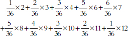
In many problems, the weighted average is computed with respect to the density; then sums must be replaced by integrals. The expected value need not be a possible value for the random variable.
Generally, a random variable will be somewhere around its expected value, but will be off (in either direction) by something like a standard error (SE) or so. If the random variable has a more or less normal distribution, there is about a 68% chance for it to fall in the range expected value – SE to expected value + SE. See normal curve; standard error.
randomization. See controlled experiment; randomized controlled experiment.
randomized controlled experiment. A controlled experiment in which subjects are placed into the treatment and control groups at random—as if by a lottery. See controlled experiment. Compare observational study.
range. The difference between the biggest and the smallest values in a batch of numbers.
rate. In an epidemiological study, the number of events, divided by the size of the population; often cross-classified by age and gender. For example, the death rate from heart disease among American men ages 55–64 in 2004 was about three per thousand. Among men ages 65–74, the rate was about seven per thousand. Among women, the rate was about half that for men. Rates adjust for differences in sizes of populations or subpopulations. Often, rates are computed per unit of time, e.g., per thousand persons per year. Data source: Statistical Abstract of the United States tbl. 115 (2008).
regression coefficient. The coefficient of a variable in a regression equation. See regression model.
regression diagnostics. Procedures intended to check whether the assumptions of a regression model are appropriate.
regression equation. See regression model.
regression line. The graph of a (simple) regression equation.
regression model. A regression model attempts to combine the values of certain variables (the independent or explanatory variables) in order to get expected values for another variable (the dependent variable). Sometimes, the phrase
“regression model” refers to a probability model for the data; if no qualifications are made, the model will generally be linear, and errors will be assumed independent across observations, with common variance, The coefficients in the linear combination are called regression coefficients; these are parameters. At times, “regression model” refers to an equation (“the regression equation”) estimated from data, typically by least squares.
For example, in a regression study of salary differences between men and women in a firm, the analyst may include a dummy variable for gender, as well as statistical controls such as education and experience to adjust for productivity differences between men and women. The dummy variable would be defined as 1 for the men and 0 for the women. Salary would be the dependent variable; education, experience, and the dummy would be the independent variables. See least squares; multiple regression; random error; variance. Compare general linear model.
relative frequency. See frequency.
relative risk. A measure of association used in epidemiology. For example, if 10% of all people exposed to a chemical develop a disease, compared to 5% of people who are not exposed, then the disease occurs twice as frequently among the exposed people: The relative risk is 10%/5% = 2. A relative risk of 1 indicates no association. For more details, see Leon Gordis, Epidemiology (4th ed. 2008). Compare odds ratio.
reliability. The extent to which a measurement process gives the same results on repeated measurement of the same thing. Compare validity.
representative sample. Not a well-defined technical term. A sample judged to fairly represent the population, or a sample drawn by a process likely to give samples that fairly represent the population, for example, a large probability sample.
resampling. See bootstrap.
residual. The difference between an actual and a predicted value. The predicted value comes typically from a regression equation, and is better called the fitted value, because there is no real prediction going on. See regression model; independent variable.
response variable. See independent variable.
risk. Expected loss. “Expected” means on average, over the various datasets that could be generated by the statistical model under examination. Usually, risk cannot be computed exactly but has to be estimated, because the parameters in the statistical model are unknown and must be estimated. See loss function; random variable.
risk factor. See independent variable.
robust. A statistic or procedure that does not change much when data or assumptions are modified slightly.
sample. A set of units collected for study. Compare population.
sample size. Also, size of sample. The number of units in a sample.
sample weights. See stratified random sample.
sampling distribution. The distribution of the values of a statistic, over all possible samples from a population. For example, suppose a random sample is drawn. Some values of the sample mean are more likely; others are less likely. The sampling distribution specifies the chance that the sample mean will fall in one interval rather than another.
sampling error. A sample is part of a population. When a sample is used to estimate a numerical characteristic of the population, the estimate is likely to differ from the population value because the sample is not a perfect microcosm of the whole. If the estimate is unbiased, the difference between the estimate and the exact value is sampling error. More generally,
estimate = true value + bias + sampling error
Sampling error is also called chance error or random error. See standard error. Compare bias; nonsampling error.
sampling frame. A list of units designed to represent the entire population as completely as possible. The sample is drawn from the frame.
sampling interval. See systematic sample.
scatter diagram. Also, scatterplot; scattergram. A graph showing the relationship between two variables in a study. Each dot represents one subject. One variable is plotted along the horizontal axis, the other variable is plotted along the vertical axis. A scatter diagram is homoscedastic when the spread is more or less the same inside any vertical strip. If the spread changes from one strip to another, the diagram is heteroscedastic.
selection bias. Systematic error due to nonrandom selection of subjects for study.
sensitivity. In clinical medicine, the probability that a test for a disease will give a positive result given that the patient has the disease. Sensitivity is analogous to the power of a statistical test. Compare specificity.
sensitivity analysis. Analyzing data in different ways to see how results depend on methods or assumptions.
sign test. A statistical test based on counting and the binomial distribution. For example, a Finnish study of twins found 22 monozygotic twin pairs where 1 twin smoked, 1 did not, and at least 1 of the twins had died. That sets up a race to death. In 17 cases, the smoker died first; in 5 cases, the nonsmoker died first. The null hypothesis is that smoking does not affect time to death, so the chances are 50-50 for the smoker to die first. On the null hypothesis, the chance that the smoker will win the race 17 or more times out of 22 is
8/1000. That is the p-value. The p-value can be computed from the binomial distribution. For additional detail, see Michael O. Finkelstein & Bruce Levin, Statistics for Lawyers 339–41 (2d ed. 2001); David A. Freedman et al., Statistics 262–63 (4th ed. 2007).
significance level. See fixed significance level; p-value.
significance test. Also, statistical test; hypothesis test; test of significance. A significance test involves formulating a statistical hypothesis and a test statistic, computing a p-value, and comparing p to some preestablished value (a) to decide if the test statistic is significant. The idea is to see whether the data conform to the predictions of the null hypothesis. Generally, a large test statistic goes with a small p-value; and small p-values would undermine the null hypothesis.
For example, suppose that a random sample of male and female employees were given a skills test and the mean scores of the men and women were different—in the sample. To judge whether the difference is due to sampling error, a statistician might consider the implications of competing hypotheses about the difference in the population. The null hypothesis would say that on average, in the population, men and women have the same scores: The difference observed in the data is then just due to sampling error. A one-sided alternative hypothesis would be that on average, in the population, men score higher than women. The one-sided test would reject the null hypothesis if the sample men score substantially higher than the women—so much so that the difference is hard to explain on the basis of sampling error.
In contrast, the null hypothesis could be tested against the two-sided alternative that on average, in the population, men score differently than women—higher or lower. The corresponding two-sided test would reject the null hypothesis if the sample men score substantially higher or substantially lower than the women.
The one-sided and two-sided tests would both be based on the same data, and use the same t-statistic. However, if the men in the sample score higher than the women, the one-sided test would give a p-value only half as large as the two-sided test; that is, the one-sided test would appear to give stronger evidence against the null hypothesis. (“One-sided” and “one-tailed” are synonymous; so are “two-sided and “two-tailed.”) See p-value; statistical hypothesis; t-statistic.
significant. See p-value; practical significance; significance test.
simple random sample. A random sample in which each unit in the sampling frame has the same chance of being sampled. The investigators take a unit at random (as if by lottery), set it aside, take another at random from what is left, and so forth.
simple regression. A regression equation that includes only one independent variable. Compare multiple regression.
size. A synonym for alpha (α).
skip factor. See systematic sample.
specificity. In clinical medicine, the probability that a test for a disease will give a negative result given that the patient does not have the disease. Specificity is analogous to 1 – α, where α is the significance level of a statistical test. Compare sensitivity.
spurious correlation. When two variables are correlated, one is not necessarily the cause of the other. The vocabulary and shoe size of children in elementary school, for example, are correlated—but learning more words will not make the feet grow. Such noncausal correlations are said to be spurious. (Originally, the term seems to have been applied to the correlation between two rates with the same denominator: Even if the numerators are unrelated, the common denominator will create some association.) Compare confounding variable.
standard deviation (SD). Indicates how far a typical element deviates from the average. For example, in round numbers, the average height of women age 18 and over in the United States is 5 feet 4 inches. However, few women are exactly average; most will deviate from average, at least by a little. The SD is sort of an average deviation from average. For the height distribution, the SD is 3 inches. The height of a typical woman is around 5 feet 4 inches, but is off that average value by something like 3 inches.
For distributions that follow the normal curve, about 68% of the elements are in the range from 1 SD below the average to 1 SD above the average. Thus, about 68% of women have heights in the range 5 feet 1 inch to 5 feet 7 inches. Deviations from the average that exceed 3 or 4 SDs are extremely unusual. Many authors use standard deviation to also mean standard error. See standard error.
standard error (SE). Indicates the likely size of the sampling error in an estimate. Many authors use the term standard deviation instead of standard error. Compare expected value; standard deviation.
standard error of regression. Indicates how actual values differ (in some average sense) from the fitted values in a regression model. See regression model; residual. Compare R-squared.
standard normal. See normal distribution.
standardization. See standardized variable.
standardized variable. Transformed to have mean zero and variance one. This involves two steps: (1) subtract the mean; (2) divide by the standard deviation.
statistic. A number that summarizes data. A statistic refers to a sample; a parameter or a true value refers to a population or a probability model.
statistical controls. Procedures that try to filter out the effects of confounding variables on non-experimental data, for example, by adjusting through statistical procedures such as multiple regression. Variables in a multiple regression
equation. See multiple regression; confounding variable; observational study. Compare controlled experiment.
statistical dependence. See dependence.
statistical hypothesis. Generally, a statement about parameters in a probability model for the data. The null hypothesis may assert that certain parameters have specified values or fall in specified ranges; the alternative hypothesis would specify other values or ranges. The null hypothesis is tested against the data with a test statistic; the null hypothesis may be rejected if there is a statistically significant difference between the data and the predictions of the null hypothesis.
Typically, the investigator seeks to demonstrate the alternative hypothesis; the null hypothesis would explain the findings as a result of mere chance, and the investigator uses a significance test to rule out that possibility. See significance test.
statistical independence. See independence.
statistical model. See probability model.
statistical test. See significance test.
statistical significance. See p-value.
stratified random sample. A type of probability sample. The researcher divides the population into relatively homogeneous groups called “strata,” and draws a random sample separately from each stratum. Dividing the population into strata is called “stratification.” Often the sampling fraction will vary from stratum to stratum. Then sampling weights should be used to extrapolate from the sample to the population. For example, if 1 unit in 10 is sampled from stratum A while 1 unit in 100 is sampled from stratum B, then each unit drawn from A counts as 10, and each unit drawn from B counts as 100. The first kind of unit has weight 10; the second has weight 100. See Freedman et al., Statistics 401 (4th ed. 2007).
stratification. See independent variable; stratified random sample.
study validity. See validity.
subjectivist. See Bayesian.
systematic error. See bias.
systematic sample. Also, list sample. The elements of the population are numbered consecutively as 1, 2, 3,…. The investigators choose a starting point and a “sampling interval” or “skip factor” k. Then, every kth element is selected into the sample. If the starting point is 1 and k = 10, for example, the sample would consist of items 1, 11, 21,…. Sometimes the starting point is chosen at random from 1 to k: this is a random-start systematic sample.
t-statistic. A test statistic, used to make the t-test. The t-statistic indicates how far away an estimate is from its expected value, relative to the standard error. The expected value is computed using the null hypothesis that is being tested.
Some authors refer to the t-statistic, others to the z-statistic, especially when the sample is large. With a large sample, a t-statistic larger than 2 or 3 in absolute value makes the null hypothesis rather implausible—the estimate is too many standard errors away from its expected value. See statistical hypothesis; significance test; t-test.
t-test. A statistical test based on the t-statistic. Large t-statistics are beyond the usual range of sampling error. For example, if t is bigger than 2, or smaller than −2, then the estimate is statistically significant at the 5% level; such values of t are hard to explain on the basis of sampling error. The scale for t-statistics is tied to areas under the normal curve. For example, a t-statistic of 1.5 is not very striking, because 13% = 13/100 of the area under the normal curve is outside the range from −1.5 to 1.5. On the other hand, t = 3 is remarkable: Only 3/1000 of the area lies outside the range from −3 to 3. This discussion is predicated on having a reasonably large sample; in that context, many authors refer to the z-test rather than the t-test.
Consider testing the null hypothesis that the average of a population equals a given value; the population is known to be normal. For small samples, the t-statistic follows Student’s t-distribution (when the null hypothesis holds) rather than the normal curve; larger values of t are required to achieve significance. The relevant t-distribution depends on the number of degrees of freedom, which in this context equals the sample size minus one. A t-test is not appropriate for small samples drawn from a population that is not normal. See p-value; significance test; statistical hypothesis.
test statistic. A statistic used to judge whether data conform to the null hypothesis. The parameters of a probability model determine expected values for the data; differences between expected values and observed values are measured by a test statistic. Such test statistics include the chi-squared statistic (c2) and the t-statistic. Generally, small values of the test statistic are consistent with the null hypothesis; large values lead to rejection. See p-value; statistical hypothesis; t-statistic.
time series. A series of data collected over time, for example, the Gross National Product of the United States from 1945 to 2005.
treatment group. See controlled experiment.
two-sided hypothesis; two-tailed hypothesis. An alternative hypothesis asserting that the values of a parameter are different from—either greater than or less than—the value asserted in the null hypothesis. A two-sided alternative hypothesis suggests a two-sided (or two-tailed) test. See significance test; statistical hypothesis. Compare one-sided hypothesis.
two-sided test; two-tailed test. See two-sided hypothesis.
Type I error. A statistical test makes a Type I error when (1) the null hypothesis is true and (2) the test rejects the null hypothesis, i.e., there is a false posi-
tive. For example, a study of two groups may show some difference between samples from each group, even when there is no difference in the population. When a statistical test deems the difference to be significant in this situation, it makes a Type I error. See significance test; statistical hypothesis. Compare alpha; Type II error.
Type II error. A statistical test makes a Type II error when (1) the null hypothesis is false and (2) the test fails to reject the null hypothesis, i.e., there is a false negative. For example, there may not be a significant difference between samples from two groups when, in fact, the groups are different. See significance test; statistical hypothesis. Compare beta; Type I error.
unbiased estimator. An estimator that is correct on average, over the possible datasets. The estimates have no systematic tendency to be high or low. Compare bias.
uniform distribution. For example, a whole number picked at random from 1 to 100 has the uniform distribution: All values are equally likely. Similarly, a uniform distribution is obtained by picking a real number at random between 0.75 and 3.25: The chance of landing in an interval is proportional to the length of the interval.
validity. Measurement validity is the extent to which an instrument measures what it is supposed to, rather than something else. The validity of a standardized test is often indicated by the correlation coefficient between the test scores and some outcome measure (the criterion variable). See content validity; differential validity; predictive validity. Compare reliability.
Study validity is the extent to which results from a study can be relied upon. Study validity has two aspects, internal and external. A study has high internal validity when its conclusions hold under the particular circumstances of the study. A study has high external validity when its results are generalizable. For example, a well-executed randomized controlled double-blind experiment performed on an unusual study population will have high internal validity because the design is good; but its external validity will be debatable because the study population is unusual.
Validity is used also in its ordinary sense: assumptions are valid when they hold true for the situation at hand.
variable. A property of units in a study, which varies from one unit to another, for example, in a study of households, household income; in a study of people, employment status (employed, unemployed, not in labor force).
variance. The square of the standard deviation. Compare standard error; covariance. weights. See stratified random sample.
within-observer variability. Differences that occur when an observer measures the same thing twice, or measures two things that are virtually the same. Compare between-observer variability.
z-statistic. See t-statistic.
z-test. See t-test.
General Surveys
David Freedman et al., Statistics (4th ed. 2007).
Darrell Huff, How to Lie with Statistics (1993).
Gregory A. Kimble, How to Use (and Misuse) Statistics (1978).
David S. Moore & William I. Notz, Statistics: Concepts and Controversies (2005).
Michael Oakes, Statistical Inference: A Commentary for the Social and Behavioral Sciences (1986).
Statistics: A Guide to the Unknown (Roxy Peck et al. eds., 4th ed. 2005). Hans Zeisel, Say It with Figures (6th ed. 1985).
Reference Works for Lawyers and Judges
David C. Baldus & James W.L. Cole, Statistical Proof of Discrimination (1980 & Supp. 1987) (continued as Ramona L. Paetzold & Steven L. Willborn, The Statistics of Discrimination: Using Statistical Evidence in Discrimination Cases (1994) (updated annually).
David W. Barnes & John M. Conley, Statistical Evidence in Litigation: Methodology, Procedure, and Practice (1986 & Supp. 1989).
James Brooks, A Lawyer’s Guide to Probability and Statistics (1990).
Michael O. Finkelstein & Bruce Levin, Statistics for Lawyers (2d ed. 2001).
Modern Scientific Evidence: The Law and Science of Expert Testimony (David L. Faigman et al. eds., Volumes 1 and 2, 2d ed. 2002) (updated annually).
David H. Kaye et al., The New Wigmore: A Treatise on Evidence: Expert Evidence § 12 (2d ed. 2011) (updated annually).
National Research Council, The Evolving Role of Statistical Assessments as Evidence in the Courts (Stephen E. Fienberg ed., 1989).
Statistical Methods in Discrimination Litigation (David H. Kaye & Mikel Aickin eds., 1986).
Hans Zeisel & David Kaye, Prove It with Figures: Empirical Methods in Law and Litigation (1997).
General Reference
Encyclopedia of Statistical Sciences (Samuel Kotz et al. eds., 2d ed. 2005).


