
Integrity Lessons from the WAAS Integrity Performance Panel
TODD WALTER AND PER ENGE
Stanford University
BRUCE DeCLEENE
Federal Aviation Administration
ABSTRACT
The Wide Area Augmentation System (WAAS), a system to allow the use of the Global Positioning System (GPS) for many phases of flight within the United States, was implemented because its benefits are significant. It provides guidance throughout the national airspace. It supports approaches with vertical guidance to more runway ends in the United States than all other landing systems combined. It does this without requiring local navigational aids. It also can support procedures such as curved approaches and departures. These and other benefits motivated the effort to create and certify this new system. However, WAAS is unlike previous navigation systems fielded by the Federal Aviation Administration (FAA). Historically, the FAA has implemented relatively simple and distributed systems. Each only affects a small portion of the airspace and each is maintained independently of the others. WAAS, in contrast, is a complex and centralized system that provides guidance to the whole airspace. Consequently, the certification for WAAS proceeded very cautiously.
A unique aspect of WAAS compared to traditional terrestrial navigational aids is that it is inherently a non-stationary system. It relies on satellites that are constantly in motion and that may change their characteristics. Additionally, the propagation of the satellite signals varies with local ionospheric and tropospheric conditions. Thus, the system has differing properties over time and space. However, the system requirements apply to each individual approach. In particular, the integrity requirement, that the confidence bound fails to contain the true error in fewer than 1 in 10 million approaches, must apply to all users under all foresee-
able operational conditions. To ensure that the integrity requirement would be met, the FAA formed the WAAS Integrity Performance Panel (WIPP). The role of the WIPP is to independently assess the safety of WAAS and to recommend system improvements. To accomplish these tasks for initial certification, the WIPP had to determine how to interpret the integrity requirement for WAAS, develop algorithms to meet this requirement, and ultimately validate them.
INTRODUCTION
WAAS monitors the GPS and provides both differential corrections to improve the accuracy and associated confidence bounds to ensure the integrity. WAAS utilizes a network of precisely surveyed reference receivers located throughout the United States. The information gathered from these WAAS Reference Stations (WRSs) monitors GPS and its propagation environment in real-time. However, the WAAS designers had to be aware of the limitations of its monitoring. The measurements that it makes are corrupted by noise and biases causing certain fault modes to be difficult to detect. Because it is a safety-of-life system, WAAS must place rigorous bounds on the probability that it is in error, even under faulted conditions.
In late 1999, concerns arose over the original WAAS design and the process by which WAAS was to be proven safe. In response, the FAA created the WIPP. The WIPP is a body of GPS and system safety experts chartered to assess the system engineering and safety design of WAAS and recommend required changes. The WIPP consists of members from government (FAA, Jet Propulsion Laboratory), industry (Raytheon, Zeta, MITRE), and academia (Stanford University). They first convened in early 2000 to address the integrity and certification of WAAS.
Primarily WIPP quantified the degree to which WAAS mitigated the system vulnerabilities. Over its first two years, WIPP changed the design of several system components where the system could not satisfactorily demonstrate the required level of integrity. As each threat was addressed, WIPP built upon what it had learned.
Some of the main lessons that emerged from WIPP are:
- The aviation integrity requirement of 10–7 per approach applies in principle to each and every approach. It is not an ensemble average over all conditions.
- Validated threat models are essential both to describe what the system protects against and to quantitatively assess how effectively it provides such protection.
- The system design must be shown to be safe against all fault modes including external threats, addressing the potential for latent faults just beneath the system’s ability to detect them. This approach is unlike
conventional non-aviation differential systems that presume no failures exist unless consistency checks fail.
- The safety analysis must protect all allowed geometries. It does not protect just the all-in-view case; all subset combinations that support the operation must be safe as well.
- The small numbers associated with integrity analysis are not intuitive. Careful analysis must take priority over anecdotal evidence.
These lessons will be described in greater detail. Of these lessons, the need for threat models is the most important and originally was the most lacking. Threat models describe events or conditions that may cause harm to the user. In this case, harm is referred to as hazardously misleading information (HMI). It is defined as a true error that is larger than the guaranteed protection level (PL). WAAS provides differential corrections that are applied to the received pseudoranges from GPS. At the same time, confidence bounds are also supplied to the user. These bounds are combined with the geometry of satellites visible to the user to calculate the PL. In order to use the calculated position for navigation, the PL must be small enough to support the operation. The user only has real-time access to the PL, not the true error. Thus, HMI arises if the user has been told that the error in position is small enough to support the operation, but in fact, it is not.
The threat models must describe all known conditions that could cause the true errors to exceed the predicted confidence bounds. Having a comprehensive list is essential to achieving the required level of safety and it also drives the system design. Additionally, restricting the scope of the threats is necessary for practical reasons. It is not possible to create a system that can protect against every conceivable threat. Fortunately, many such threats are either unphysical or extremely improbable. Restricting threats to those that are sufficiently likely is necessary for creating a practical system.
INTEGRITY REQUIREMENT
The integrity requirement for precision approach guidance (down to 200’ above the ground) is 1-2 × 10⁻⁷ per approach (ICAO, 2006). There is a general understanding that this probabilistic requirement applies individually to every approach. This definition is further refined in the WAAS specification (2: FAA-E-2892C WAAS Specification) as applying at every location and time in the service volume. It is not acceptable for one airport to have less integrity simply because a different aircraft hundreds of miles away has margin against the requirement. Similarly, with the non-stationary characteristics arising from effects such as the orbiting satellites, it is not appropriate for operations to continue during an interval when the integrity requirement is not met, just because it is exceeded for the rest of the day. Generally, this can be restated as meaning that the probability of hazardously misleading information (HMI) must be at or below
1 × 10⁻⁷ for an approach at the worst time and location in the service volume for which the service is claimed to be available. Despite this apparent understanding, a more detailed discussion of the interpretation is instructive.
The integrity requirement is that the positioning error (PE) must be no greater than the confidence bound, known as the PL, beyond the specified probability. Confusion may result because the requirement is probabilistic, yet at the worst time and place, the errors appear deterministic. Instead, the requirement should be viewed as applying to a hypothetical collection of users under essentially identical conditions. The collection of users, referred to as the ensemble, must be hypothetical in this case because satellite navigation systems and their associated errors are inherently non-stationary. Any true ensemble would average over too many different conditions, combining users with high and low risk. Thus, we must imagine an ensemble of users, for each point in space and time, whose errors follow probability distributions specific to that point.
Of course, there can only be one actual user at a given point in space and time. That user will experience a specific set of errors that combine to create the position error. These errors are comprised of both deterministic and stochastic components. The distinction is that if we could replicate the conditions and environment for the user, the deterministic components would be completely repeatable. Thus, these errors would be common mode; all users in our ensemble would suffer them to the same degree. On the other hand, stochastic errors such as thermal noise would differ for each user in our ensemble. Overall, these components combine to form a range of possible errors whose magnitudes have differing probability. When we look at a very large number (approaching infinity) of hypothetical users in the ensemble, some will have errors that exceed the protection level while most will not. The fraction of users that exceed the PL can be used to determine the probability of an integrity failure under those conditions.
The difficult aspect of applying this philosophy is defining equivalent user conditions and then determining the error distributions. A circular definition is that user conditions can be called equivalent if they carry the same level of risk. A more practical approach is to exploit prior knowledge of the error sources. For example, if it were known that an error source only has a definite temperature dependency, then the ensembles should be formed over all users in narrow temperature ranges. The error distributions and probability of exceeding the PL would be calculated for each ensemble, and the integrity requirement would have to be met for the most difficult case for which availability is claimed. Unfortunately, true error sources usually have multiple dependencies, and these dependencies are different between the various error sources. Thus, the ensembles may need to be formed over narrow ranges of numerous parameters. However, great care must be taken because, if certain dependencies are not properly recognized, the ensembles may unknowingly average over different risk levels.
The restatement of the requirement that it applies to the worst time and location is misleading because it is acceptable to average against certain condi-
tions. Some events may be sufficiently rare to ignore altogether. If, under similar conditions, the a priori likelihood is well below 1 × 10⁻⁷ per approach (considering exposure time to the failure), then there may not be any need to provide additional protection. The worst time and place should not be viewed as when and where this unlikely event occurs. The event need only be considered if it is sufficiently likely to occur, if when and where it is most likely to occur can be predicted ahead of time, or if it is strongly correlated with an observable. Even if the event is not sufficiently rare to be ignored, its a priori probability may be utilized provided the event remains unpredictable and immeasurable. Thus, the conditions where the event is present may be averaged with otherwise similar conditions without the event. Taking advantage of such a priori probabilities must be approached very cautiously on a case-by-case basis.
The goal is to ensure that all users are exposed to risk at no greater than the specified rate of 10–7 per approach. Thus, ensembles that cannot be correlated in some way with user behavior or an observable parameter do not make sense. For example, users may tend to fly to the same airport at the same time of day or during a certain season. Therefore, an ensemble of all users with a specific geometry at a certain location and certain time of day, but theoretically infinitely extended forwards and backwards over adjacent days, is reasonable. On the other hand, an ensemble of all users whose thermal noise consists of five-sigma errors aligned in the worst possible direction is neither realistic nor practical. The latter example attempts to combine rare and random events into a unifying ensemble that cannot be made to correspond to user behavior or to any practically measurable quantity. In general, conditions leading to high risk that are both rare and random can be averaged with lower risk conditions. The requirement for rarity seeks to assure that users do not receive multiple exposures to the high-risk condition, while the requirement for randomness seeks to avoid a predictable violation of the integrity requirement. Correlation with conceivable user behavior must be a determining factor when deciding whether or not to average the risk. Similarly, a correlation with a system observable should be exploited to protect the user when performance goes out of tolerance.
Deciding how to define the ensembles provides the necessary information for determining the error distributions. Components will largely be divided into noise-like contributions, with some spread in their values, and bias-like contributions whose values are seen as fixed although unknown. Although many of these error sources may be deterministic, practically they may need to be described in stochastic terms. Many error sources fall into this category, including ionosphere, troposphere, and multipath. If we knew enough about the surrounding environments, we could predict their effects for each user. However, because it is usually not practical to obtain this information, it may be acceptable to view these effects as unpredictable as long as their effects cannot be correlated with user behavior.
Knowledge of the error characteristics is very important in evaluating system design. While impossible to know fully, many important characteristics such as
dependencies may be recognized. This knowledge allows proper determination of the error distributions. After defining the individual distributions, the correlations between them must be established. Many deterministic error sources may affect multiple ranging sources simultaneously. Correlated deterministic errors may add together coherently for a specific user. Such effects require larger increases in the protection level than if the errors were uncorrelated. If these effects are not recognized and treated appropriately, the integrity requirement will not be met and the user will suffer excessive risk. Although the form of the protection level equations given in ICAO (2006) and FAA (2009) suggest that all error sources are independent, zero-mean, and gaussian, this is not the case under all operating conditions. Each error source must be carefully analyzed, both individually and in relation to the other sources. Only then can the appropriate confidence bounds be determined.
ERROR MODELING
Each individual error source has some probability distribution associated with it. This distribution describes the likelihood of encountering a certain error value. Ideally, smaller errors are more likely than larger errors. Generally, this is true for most error sources. The central region of most error sources can be well described by a gaussian distribution. That is, most errors are clustered about a mean (usually near zero) and the likelihood of being farther away from the mean falls off according to the well-known model. This is often a consequence of the central-limit-theorem that states that distributions tend to approach gaussian as more independent random variables are combined.
Unfortunately, the tails of the observed distributions rarely look gaussian. Two competing effects tend to modify their behavior. The first is clipping. Because there are many cross-comparisons and reasonability checks, the larger errors tend to be removed. Thus, for a truly gaussian process, outlier removal would lead to fewer large errors than would otherwise be expected. The second effect is mixing. The error sources are rarely stationary. Thus, some of the time the error might be gaussian with a certain mean and sigma and at other times have a different distribution. Such mixing may result from a change in the nominal conditions or from the introduction of a fault mode. Mixing generally leads to broader tails or large errors being more likely than otherwise expected.
The mixing causes additional problems. If the error processes were stationary, it would be possible to collect as large a data set as practical and then conservatively extrapolate the tail behavior using a gaussian or other model. However, because the distribution changes over time, it is more difficult to predict future performance based on past behavior. Furthermore, mixing leads to more complicated distributions whose tails are more difficult to extrapolate. With enough mixing, it can be very difficult to characterize the underlying distributions at all. Figure 1 is an example of a mixed distribution. The majority
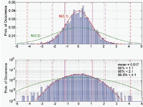
FIGURE 1 Simulated probability distribution composed of a mixed gaussian: 2,900 points with unity variance and 100 points with a variance of four. The top and bottom graphs are the same data displayed on a linear scale (top) and log-scale (bottom).
of the data points are selected from a zero-mean gaussian with unity variance. A few of the points are selected from a zero-mean gaussian with a variance of four. This plot contains some very typical features of the real data we collect. The majority of the data conforms very well to a gaussian model, while the tails usually contain outliers. Sampling issues are usually significant because it is very difficult to obtain large amounts of independent data. Thus, just by looking at the graph it is difficult to determine the actual distribution.
The central-limit-theorem causes error distributions to approach gaussian as several independent sources are combined. Certainly, the main body of collected data tends to be gaussian in appearance. The tails are more difficult to discern. A generalized mixed gaussian description is appropriate. Here, the errors can be described as gaussian where the mean and variance are also drawn from some joint probability distribution.
ε ![]() N(μ,σ)
N(μ,σ)
μ,σ ![]() pr(M,Σ)
pr(M,Σ)
At any given instant, the error is gaussian, but its mean and variance have some uncertainty. By understanding the extent of the possible means and variances we can overbound the worst-case. Additional information ideally allows us to partition the space and distinguish when larger bounds are needed versus when smaller ones can be provided.
Nominally, we expect the distribution to be zero-mean and have some well-defined variance. Some small fraction of the time the error may still be zero-mean, but have a larger variance as depicted in Figure 1. During a fault mode the mean may grow in magnitude, but the variance may stay roughly the same as nominal (of course other variances are possible). Restricting the error distribution to this class distribution allows the analysis to become tractable.
Of course, it is impossible to truly know the real distribution, particularly to 10–7 confidence. The use of a model like this must be accepted by a body of experts such as the WIPP who can assert that it is valid based on physical knowledge of the system design, supporting data, and simulation. This combination is essential for describing the tail behavior. A physical understanding of the error process is essential to describing expected behavior. Data must be collected in sufficient quantity and under many conditions. The physical knowledge must be exploited to determine what the worst-case conditions are and how data should be reduced. For example, severe ionospheric behavior is correlated with solar events and magnetic disturbances. Data must be collected during some of the most extreme operating conditions. Finally, simulation may be used to confirm that the models constructed are consistent with the observations.
Physical knowledge of the system is essential. Any information on the physical processes behind the error source can be used to separate mixtures and create better-defined distributions. For example, multipath can be related to the surrounding environment. Large reflections tend to occur at lower elevation angles. Partitioning data by elevation angles may reduce mixing. Changes to multipath can be related to changes in satellite position and to changes in the environment. Excessive multipath can sometimes be related to specific reflectors. Additionally, the magnitude of multipath errors can be bounded by limiting the number of reflectors and strength of the reflected signals.
Data are also essential. The data must be sufficient to support assumptions or validate system performance to the degree to which the safety of the system relies on that data. It is not sufficient to collect a day or two of randomly selected data; data collected over many days under extreme conditions are needed. Examples include tropospheric data from many different climates, ionospheric data from the worst times in the 11-year solar cycle, multipath data from the most cluttered environments, etc. Rare events are unlikely to be captured in small data sets. Large data sets, taken over long time periods, are more likely to capture postulated events. Having data containing these events provides better insight into their effect.
THREAT MODELS
Threat models describe the anticipated events that the system must protect the user against and conditions during which it must provide reliably safe confidence bounds. Each threat model must describe the specific nature of the threat, its magnitude, and its likelihood. Together, the various threat models must be comprehensive in describing all reasonable conditions under which the system might have difficulty protecting the user. Ultimately they form a major part of the basis for determining if the system design meets its integrity requirement. Each individual threat must be fully mitigated to within its allocation. Only when it can be shown that each threat has been sufficiently addressed can the system be deemed safe.
WAAS was developed primarily to address existing threats to GPS. However, it also runs the risk of introducing threats in absence of any GPS fault. By necessity, it is a complex system of hardware and software. Included in any threat model must be self-induced errors. Some of these errors are universal to any design while others are specific to the implementation. For example, the software design assurance of WAAS reference receivers was based on market availability of equipment, so reference receivers’ software faults are a unique threat that has to be mitigated through system integrity monitoring. The following is a high-level list of generic threats. While it is not comprehensive, it does include the most significant categories either for magnitude of effect or likelihood. There are numerous other threats that have a smaller effect, are less likely, or are implementation specific.
High-Level Threat List
• Satellite
— Clock/ephemeris error
— Signal deformation
— Code carrier incoherency
• Ionosphere
— Local non-planar behavior
o Well-sampled
o Undersampled
• Troposphere
• Reference receiver
— Multipath
— Thermal noise
— Antenna bias
— Survey errors
— Receiver errors
• Master station
— Space vehicle (SV) clock/ephemeris estimation errors
— Ionospheric estimation errors
— SV Tgd estimation errors
— Receiver IFB estimation errors
— WRS clock estimation errors
— Communication errors
— Broadcast errors
• User errors
The following sections provide greater detail for each threat, although the true details depend on implementation and must be decided by the service provider.
SV Clock/Ephemeris Estimation Errors
Satellites suffer from nominal ephemeris and clock errors even when there are no faults in the GPS system (Creel et al., 2007; Heng et al., 2011; Jefferson and Bar-Sever, 2000; Warren and Raquet, 2002). Additionally, the broadcast GPS clock and ephemeris information may contain significant errors in the event of a GPS system fault or erroneous upload. Such faults may create jumps, ramps, or higher-order errors in the GPS clock, ephemeris, or both (Gratton et al., 2007; Hansen et al., 1998; Heng et al., 2010; Rivers, 2000; Shank and Lavrakas, 1993). Such faults may be created by changes in state of the satellite orbit or clock or simply due to the broadcasting of erroneous information. Either the user or the system may also experience incorrectly decoded ephemeris information.
The user differential range error (UDRE), a term designed to describe residual satellite errors, must be sufficient to overbound the residual errors in the corrected satellite clock and ephemeris.
Signal Deformations
The International Civil Aviation Organization (ICAO) has adopted a threat model to describe the possible signal distortions that may occur on the GPS L1 CA code (ICAO, 2006). These distortions will lead to biases that depend upon the correlator spacing and bandwidth of the observing receivers. Such biases would be transparent to a network of identically configured receivers (Hsu et al., 2008; Phelts et al., 2009; Wong et al., 2010).
The UDRE must be sufficient to overbound unobservable errors caused by signal deformation. Unobservable errors are those that cannot be detected to the required level of integrity.
Code-Carrier Incoherency
Another threat is that a satellite may fail to maintain the coherency between the broadcast code and carrier. This fault mode occurs on the satellite and is unrelated to incoherence caused by the ionosphere. This threat causes either a step
or a rate of change between the code and carrier broadcast from the satellite. This threat has never been observed on the GPS L1 signals, but it has been observed on WAAS geostationary signals and on the GPS L5 signal (Gordon et al., 2010; Montenbruck et al., 2010).
The UDRE must be sufficient to overbound unobservable errors caused by incoherency. Unobservable errors are those that cannot be detected to the required level of integrity.
Ionosphere and Ionospheric Estimation Errors
The majority of the time, mid-latitude ionosphere is easily estimated and bounded using a simple local planar fit. However, periods of disturbance occasionally occur where simple confidence bounds fall significantly short of bounding the true error (Walter et al., 2001). Additionally, in other regions of the world, in particular equatorial regions, the ionosphere often cannot be adequately described by this simple model (Klobuchar et al., 2002; Rajagopal et al., 2004). Some of these disturbances can occur over very short baselines, causing them to be difficult to describe even with higher-order models. Gradients larger than 3 m of vertical delay over a 10 km baseline have been observed, even at midlatitude (Datta-Barua et al., 2002, 2010).
The broadcast ionospheric grid format specified in the Minimum Operational Performance Standards (MOPS)1 also limits accuracy and integrity. The simple two-dimensional model and assumed obliquity factor may not always provide an accurate conversion between slant and vertical ionosphere. There will also be instances where the five-degree grid is too coarse to adequately describe the structure of the surrounding ionosphere.
There are times and locations where the ionosphere is very difficult to model. This problem may be compounded by poor observability (Sparks et al., 2001; Walter et al., 2004). Ionospheric Pierce Point (IPP) placement may be such that it fails to sample important ionospheric structures. This may result from the intrinsic layout of the reference stations and satellites, or from data loss through station, satellite, or communication outages. As a result, certain ionospheric features that invalidate the assumed model can escape detection.
Finally, because the ionosphere is not a static medium, there may be large temporal gradients in addition to spatial gradients. Rates of change as large as four vertical meters per minute have been observed at mid latitudes (Datta-Barua et al., 2002).
The grid ionospheric vertical error (GIVE), a term designed to describe residual ionospheric errors, must account for inadequacies of the assumed ionospheric model, restrictions of the grid, and limitations of observability. The GIVE must be sufficient to protect against the worst possible ionospheric disturbance
____________
1 WAAS Minimum Operational Performance Specification (MOPS), RTCA document DO-229D.
that may be present in that region given the IPP distribution. Additionally, since each ionospheric correction does not time out until after 10 minutes, the GIVE and the old but active data (OBAD) terms must protect against any changes in the ionosphere that can occur over that time scale.2 Because the physics of the ionosphere are incompletely understood, the most practical ionospheric threat models are heavily data driven and contain a large amount of conservatism.
Tropospheric Errors
Tropospheric errors are typically small compared to ionospheric errors or satellite faults. Historical observations were used to formulate a model and analyze deviations from that model (Collins and Langley, 1998). A very conservative bound was applied to the distribution of those deviations. The model and bound are described in the MOPS and Standard and Recommended Procedures (SARPS) (ICAO, 2006).3 These errors may affect the user both directly through their local troposphere and indirectly through errors at the reference stations that may propagate into satellite clock and ephemeris estimates. The user protects against the direct effect using the specified formulas.
The master station must ensure that the UDRE adequately protects against the propagated tropospheric errors and their effect on satellite clock and ephemeris estimates. Of particular concern are the statistical properties of these error sources. These errors may be correlated for long periods and will produce correlated errors across all satellites at a reference station and each receiver at the reference station.
Multipath and Thermal Noise
Multipath is the most significant measurement error source. It limits the ability to estimate the satellite and ionospheric errors. It depends upon the environment surrounding the antenna and the satellite trajectories. While many receiver tracking techniques can limit its magnitude, its period can be 10 minutes or greater (Shallberg and Sheng, 2008; Shallberg et al., 2001). Additionally, it contains a periodic component that repeats over a sidereal day. Thus, severe multipath may be seen repeatedly for several days or longer.
Because all measurements that form the corrections and the UDREs and GIVEs are affected by multipath, great care must be used to bound not only its maximum extent but also its other statistical characteristics (e.g., non-gaussian, non-white, periodic). There is potential for correlation between measurements and between antennas at a single reference site. Additionally the local environment may change either due to meteorological conditions (snow, rain, ice) or physical changes (new objects or structures placed nearby).
____________
2 Ibid.
3 Ibid.
If carrier smoothing is used to mitigate multipath, then robust cycle slip detection is essential. Half integer cycle slips have been observed on many different types of receivers. In one case, several half cycle slips were observed in the same direction each several minutes apart resulting in a several meter error. Cycle slip detection must be able to reliably catch unfortunate combinations of L1 and L2 half and full integer cycle slips in order to achieve an unbiased result.
Antenna Bias
Look-angle dependent biases in the code phase on both L1 and L2 are present on reference station and GPS satellite antennas (Haines et al., 2005; Shallberg and Grabowski, 2002). These biases may be several tens of centimeters. In the case of at least one reference station antenna, they did not become smaller at higher elevation angle. These biases are observable in an anechoic chamber but more difficult to characterize in operation. They may result from intrinsic antenna design as well as manufacturing variation.
While the particular orientation of each antenna and bias may be random, it is also static. Therefore, there may exist some points in the service volume where the biases tend to add together coherently consistently. Thus, these locations will experience this effect day after day. To protect these regions, the biases should be treated pessimistically as though they are all nearly worst-case and coherent. Calibration may be applied, although individual variation, the difficulty of maintaining proper orientation, and the possibility of temporal changes, hamper its practicality.
Survey Errors
Errors in the surveyed coordinates of the antenna code phase center can affect users in the same manner as antenna biases. However, survey errors tend to be much smaller in magnitude and cancel between L1 and L2.
These errors can typically be lumped in with antenna bias protection terms and mitigated in the same manner.
Receiver Errors
The receivers themselves can introduce errors through false lock or other mechanisms, including hardware failure (GPS receiver, antenna, atomic frequency standard) or software design error (tracking loop implementation).
These may be mitigated through the use of redundant and independent receivers, antennas, and clocks at the same reference station (Haines et al., 2005). However, the UDRE and GIVE must still protect against small errors that may exist up to the size of the detection threshold.
Interfrequency Bias Estimation Errors
For internal use, the correction algorithms often need to know the hardware differential delay between the L1 and L2 frequencies. These are referred to as Tau group delay (Tgd) for the bias on the satellite and IFB for the inter-frequency bias in the reference station receivers. These values are typically estimated in tandem with the ionospheric delay estimation (Wilson et al., 1999). Although these values are nominally constant, there are some conditions under which they may change their value. One method is component switching, if a new receiver or antenna is used to replace an old one, or if different components or paths are made active on a satellite. Another means is through thermal variation either at the reference station or on the satellite as it goes through its eclipse season. Finally, component aging may also induce a slow variation.
The estimation process may have difficulty in distinguishing changes in these values from changes in the ionosphere. The steady state bias value and step changes may be readily observable, but slow changes comparable to the ionosphere may be particularly difficult to distinguish. Ionospheric disturbances that do not follow the assumed model of the ionosphere may also corrupt the bias estimates. The UDREs and GIVEs must bound the uncertainty that may result from such estimation errors.
Receiver Clock Estimate Errors
Similarly, the satellite correction algorithm must estimate and remove the time offsets between the reference station receivers. These differences are nominally linear over long times for atomic frequency standards. However, component replacement or failure may invalidate that model.
Nominally, these differences are easily separated; however, reference station clock failures and/or satellite ephemeris errors may make this task more difficult. The UDRE must protect against errors that may propagate into the satellite clock and ephemeris correction due to these errors. Particular attention must be paid to correlations that may result from this type of misestimation
ALL-IN-VIEW AND SUBSET GEOMETRIES
The HMI requirement is specified in the position domain, yet WAAS broadcasts values in the range/correction domain. The users combine the corrections and confidences with their geometry to form the position solution and protection level. Exactly which corrections and satellites are used is known only to the user. Therefore, how the position error depends on the residual errors is known only to the users. WAAS cannot monitor only in the position domain and fully protect its users. Errors may vary with location, causing users to have different values, and users may be using different satellites to estimate their position. A combination of position domain and range/correction domain monitoring is most efficient.
To see this effect we can look at a specific user geometry. This example was created using Stanford’s Matlab Algorithm Availability Simulation Tool (MAAST), which can be used to simulate WAAS performance (Jan et al., 2001). The user has eight satellites in view as shown in Table 1. Figure 2 shows the elevations and azimuths of the satellites along with their pseudo-random noise (PRN) identification number. Table 1 also shows the PRN, elevation, azimuth, and
TABLE 1 Satellite Elevation and Azimuth Angles, Confidence Bounds, and Projection Matrix Values Both for the All-In-View Solution and Without PRN 8
| PRN | EL | AZ | σi | S3i | s3i without PRN 8 |
| 2 | 45.8º | -32.3º | 2.34 m | 0.595 | 0.451 |
| 5 | 11.2º | -76.8º | 10.10 m | 0.258 | 0.437 |
| 6 | 36.6º | 48.4º | 2.32 m | 0.162 | 2.005 |
| 8 | 9.98º | 73.0º | 3.74 m | 1.000 | - |
| 9 | 61.4º | 28.5º | 2.03 m | -1.928 | -3.087 |
| 15 | 32.8º | 151.0º | 6.89 m | -0.015 | 0.174 |
| 21 | 42.3º | -136.0º | 4.83 m | 0.066 | -0.003 |
| 122 | 40.6º | 120.1º | 6.19 m | -0.139 | 0.022 |
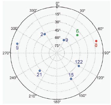
FIGURE 2 Satellite elevation and azimuth values for a standard skyplot. PRN 8 is a low elevation satellite that if not included in the solution dramatically changes the influence of PRN 6.
1-sigma confidence bound (σi). In addition, the fifth column shows the dependence of the vertical error to a pseudorange error on that satellite, s3i. S is the projection matrix and is defined as S = (GTWG)-1GTW, where G is the geometry matrix and W is the weighting matrix, see Appendix J of the WAAS Minimum Operational Performance Specification (MOPS) (RTCA document DO-229D). This term multiplies the error on the pseudorange to determine the contribution to the vertical error. Thus a 1 m ranging error on PRN 2 would create a positive 0.595 m vertical error for the user with this combination of satellites and weights. The final column in Table 1 shows the projection matrix values if PRN 8, a low elevation satellite, is not included in the position solution.
With the all-in-view solution, the user has a vertical protection level (VPL) of 33.3 m (and horizontal protection level (HPL) = 20.4 m). When PRN 8 is dropped, the VPL increases to 48.6 m (HPL = 20.5 m). Both values are below the 50 m vertical alert limit (VAL) required for the localizer-precision with vertical guidance (LPV) procedure (Cabler and DeCleene, 2002). Either solution could be used for vertical guidance. Notice that the vertical error dependency changes dramatically with the loss of PRN 8. In particular, PRN 6, which had little influence over the all-in-view solution, now has a very strong impact on this subset solution. Also notice that the other values change as well. PRNs 2, 21, and 122 lose influence while PRNs 5, 6, 9, and 15 become more important. More surprisingly, the influences of PRNs 15, 21, and 122 change sign; therefore, what was a positive error for the all-in-view solution becomes a negative error for this particular subset.
The changes in the s3i values with subset or superset position solutions limit the ability to verify performance exclusively in the position domain. For example, if PRN 6 had a 25 m bias on its pseudorange, it would lead to a vertical error of greater than 50 m with PRN 8 missing, but just over 4 m for the all-in-view solution. A position domain check with all satellites would not be concerned with a 4 m bias compared to a 33.3 m VPL. Thus, one would be inclined to think that no fault was present. However, the user unfortunate enough to lose PRN 8 would suffer a 50 m bias, large enough to cause harm. A 25 m bias would be more than a 10-sigma error in the range domain and thus is easily detectable. Therefore, it is the combination of range and position domain checks that protect users with different combinations of satellites. It is also possible to work exclusively in the position domain by using subset solutions; however, that approach may be numerically more intensive when considering a wide area system that must consider users throughout the service volume.
There is nothing unique about this particular geometry. To investigate how position errors can hide for one combination of satellites and be exposed for another, we set MAAST to look for subset solutions that had very different s3i values in their subset solutions. We restricted the search to geometries that had VPLs below 40 m for all-in-view and then only investigated subsets with VPLs below 50 m. Of the 3,726 geometries investigated, only 2 did not change S3i values by more than 40 percent.
To better illustrate the effect, the remaining 3,724 geometries had biases placed on the satellite with the largest change. Each bias was chosen such that it would lead to a 50 m positioning bias in the subset solution (a 25 m bias on PRN 6 in the example above). Each pseudorange was also assigned a zero-mean gaussian error with a standard deviation of one-half of its 1-sigma confidence bound (column four of Table 1). The broadcast WAAS confidence bounds are approximately three times larger than the nominal no-fault values (this inflation is necessary to protect against fault modes). We then calculated position errors and VPLs for both the all-in-view and subset solutions. The results are plotted in standard triangle charts (Figures 3 and 4).
Figure 3 is similar in appearance to a nominal triangle chart except the VPLs are clipped at 40 m because of our selection process and the position errors are worse than normal because of the injected error on the single satellite. However, the position errors are all below the VPL and the aggregate is not obviously biased. An observer might be inclined to believe that the system is functioning safely based on this chart. However, Figure 4 shows that the same errors and biases, but with a slightly different geometry, obviously create unsafe behavior. The subset solution removes satellites that were masking the bias for each case. The result is an obviously faulted triangle chart. Thus, a triangle chart without obvious faults, Figure 3, is no guarantee of a safe system, as evidenced by Figure 4. This has been demonstrated for real system data with much smaller biases (Sakai et al., 2010).
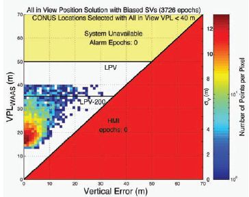
FIGURE 3 The triangle plot for all-in-view solutions including one biased satellite in each is shown. Here each bias is deweighted by the other satellites. No obvious problems are evident in this chart.
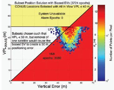
FIGURE 4 The triangle plot for the subset solutions that expose each biased satellite is shown. Here the biases are exposed as being hazardous for the user. This demonstrates the importance of checking each subset or in the range domain.
This simulation was pessimistic in its construction because the minimum unacceptable error was placed on the most sensitive satellite. On the other hand, the geometries were chosen at random and do not have any unique subset characteristics. The lesson is that it is not sufficient to observe a particular set of position solutions. The most effective method is to combine position domain monitoring with range domain monitoring.
SMALL NUMBERS AND INTUITION
The integrity requirement of 10–7 is an incredibly small number. In fact, it has to be; there have been more than 107 landings per year in the United States each year for the past 10 years.4 Granted, only a small fraction of these are instrument landings in poor visibility; however, a larger risk value could have a noticeable effect on the overall accident rate. Furthermore, air traffic is expected to increase over the coming years. To reduce the total number of accidents while increasing the number of flights requires lowering the risk per operation. Satisfying and exceeding the WAAS integrity requirement is part of that overall strategy.
____________
4 Statistics gathered from National Transportation Safety Board web page, http://www.ntsb.gov/aviation, includes parts 121 and 135 civil commercial scheduled and unscheduled landings (does not include general aviation or military operations or unscheduled commuter operations).
It is hard to imagine the exceedingly small probability of 1 part in 10 million. By design, no individual will sample anything approaching that number of approaches. At most, an individual will sample on the order of tens of thousands of approaches. The vast majority of people will experience far fewer. Additionally, that individual will mostly experience nominal conditions and rarely the unusual events, such as ionospheric disturbances, where WAAS still has to meet 10–7. Thus, personal experience is only sensitive to 10–4 at most. It is because so many flight operations take place under such a variety of conditions that WAAS needs to extend integrity to 10–7. The full population of air travelers samples the system every year in a more thorough way than any individual can in a lifetime.
WAAS is specifically in place to protect against rare events, events that one will infrequently encounter. As a result, the situations that WAAS is designed to protect against run counter to our intuition. It is tempting to say that many of the faults listed in this paper are sufficiently unlikely to occur that we do not need to worry about them. However, when attempting to quantify the probability of occurrence we often find that it is greater than 10–7. Further, because we must account for the probability of any fault occurring, specific faults are assigned sub-allocations much smaller than the full 10–7 allowance for all faults. Even a fault that occurs once per century has greater than a 10–7 chance of affecting a user in any given hour. Therefore we cannot rely solely on our observational history to convince ourselves that the system is safe.
By necessity, WAAS must work with very small numbers, probabilities of 10–7 and below. These probabilities are outside of personal experience and intuition. Events that seem unlikely must have an upper bound calculated for them. They should not simply be dismissed out of hand. Until one does the calculation they may not be able to distinguish between probabilities of 10–4 and a 10–7.
CONCLUSIONS
Augmentations systems for aviation are very different from conventional differential GPS. They are supplementing and ultimately replacing proven navigational aids whose safety has been demonstrated over many years of operational experience. Consequently their safety must be proven before they are put into service. Over the course of documenting the proof of safety, the WIPP learned many important lessons. Chief among these was the use of threat models. Threat models define our fault modes, how they manifest themselves, and how likely they are to occur. They describe what we must protect against. A well-defined threat model permits a quantitative assessment of the mitigation strategy. The quantitative assessment as opposed to a qualitative assessment is essential to establishing 10–7 integrity.
The development and validation of the threat models is one of the most important but challenging tasks in the certification. These models are created from a combination of known physical behavior, data, and simulation. The data
are very important components of this development, but it is hard to know how much data is required. The data should include all expected behaviors of the threat. The known physics can guide the initial data collection, but more data will likely be required based upon behaviors that are found in the initial set. For example, it was well-known that the ionosphere has an 11-year cycle and that it was essential to collect data from near the maximum; however, we also observed severe storm behavior that required special data collection to adequately characterize the threat.
Another key lesson is the application of the 10–7 integrity requirement to each approach. Rather than averaging over conditions with different risk levels, we must overbound the conditions describing the worst allowable situation. A priori probabilities may be used only for events that are infrequent, unpredictable, and unobservable. For example, ionospheric storms occur with certainty; therefore the system must provide at least 10–7 integrity while ionospheric disturbances are present. However, the onset time, exactly when the mid-latitude ionosphere will transition from a period of quiet to a disturbed state, is both rare and random. Thus, we may apply an a priori to that brief period of time when the ionosphere may be disturbed, but we have not yet detected it. This lesson affects how we view all of our a priori failure rates and probability distributions.
ACKNOWLEDGMENTS
The work for this paper was supported by the FAA Global Navigation Satellite System Program Office. The authors gratefully acknowledge the contributions from the other WIPP members.
REFERENCES
Cabler, H., and B. DeCleene. 2002. LPV: New, Improved WAAS Instrument Approach. Pp. 1013– 1021 in Proceedings of ION GPS-2002, Portland, Ore., September 2002. Manassas, Va.: ION.
Collins, J.P., and R.B. Langley. 1998. The Residual Tropospheric Propagation Delay: How Bad Can It Get? Pp. 729–738 in Proceedings of ION GPS-98, Nashville, Tenn., September 1998. Manassas, Va.: ION.
Creel, T., A.J. Dorsey, P.J. Mendicki, J. Little, R.G. Mach, and B.A. Renfro. 2007. Summary of Accuracy Improvements from the GPS Legacy Accuracy Improvement Initiative (L-AII). Pp. 2481–2498 in Proceedings of the 20th International Technical Meeting of the Satellite Division of The Institute of Navigation (ION GNSS 2007), Fort Worth, Tex., September 2007. Manassas, Va.: ION.
Datta-Barua, S., T. Walter, S. Pullen, M. Luo, and P. Enge. 2002. Using WAAS Ionospheric Data to Estimate LAAS Short Baseline Gradients. Pp. 523–530 in Proceeding of ION NTM, San Diego, Calif., January 2002. Manassas, Va.: ION.
Datta-Barua, S., J. Lee, S. Pullen, M. Luo, A. Ene, D. Qiu, G. Zhang, and P. Enge. 2010. Ionospheric threat parameterization for local area GPS-based aircraft landing systems. AIAA Journal of Aircraft 47(4):1141–1151.
FAA (Federal Aviation Administration). 2009. FAA Specification Wide Area Augmentation System. FAA-E-2892C. Washington, D.C.: FAA. Available online at http://www.faa.gov/about/office_org/headquarters_offices/ato/service_units/techops/navservices/gnss/library/documents/.
Gordon, S., C. Sherrell, and B.J. Potter. 2010. WAAS Offline Monitoring. Pp. 2021–2030 in Proceedings of the 23rd International Technical Meeting of the Satellite Division of the Institute of Navigation (ION GNSS 2010), Portland, Ore., September 2010. Manassas, Va.: ION.
Gratton, L., R. Pramanik, H. Tang, and B. Pervan. 2007. Ephemeris Failure Rate Analysis and Its Impact on Category I LAAS Integrity. Pp. 386–394 Proceedings of the 20th International Technical Meeting of the Satellite Division of the Institute of Navigation (ION GNSS 2007), Fort Worth, Tex., September 2007. Manassas, Va.: ION.
Haines, B., Y. Bar-Sever. W. Bertiger, S. Byun, S. Desai, and G. Hajj. 2005. GPS Antenna Phase Center Variations: New Perspectives from the GRACE Mission. Presentation at Dynamic Planet 2005, Cairns, Australia. Available online at http://wwwrc.obs-azur.fr/ftp/gmc/swt/Bruce/Haines_IAG.ppt.
Hansen, A., T. Walter, D. Lawrence, and P. Enge. 1998. GPS Satellite Clock Event of SV#27 and Its Impact on Augmented Navigation Systems. Pp. 1665–1674 in Proceedings of ION GPS-98, Nashville, Tenn., September 1998. Manassas, Va.: ION.
Heng, L., G.X. Gao, T. Walter, and P. Enge. 2010. GPS Signal-in-Space Anomalies in the Last Decade: Data Mining of 400,000,000 GPS Navigation Messages. Pp. 3115–3122 in Proceedings of the 23rd International Technical Meeting of the Satellite Division of the Institute of Navigation (ION GNSS 2010), Portland, Ore., September 2010. Manassas, Va.: ION.
Heng, L., G.X. Gao, T. Walter, and P. Enge. 2011. Statistical Characterization of GPS Signal-In-Space Errors. Pp. 312–319 in Proceedings of the 2011 International Technical Meeting of the Institute of Navigation, San Diego, Calif., January 2011. Manassas, Va.: ION.
Hsu, P.H., T. Chiu, Y. Golubev, and R.E. Phelts. 2008. Test Results for the WAAS Signal Quality Monitor. Pp. 263–270 in Proceedings of IEEE/ION PLANS 2008, Monterey, Calif., May 2008. Manassas, Va.: ION.
ICAO (International Civil Aviation Organization). 2006. International Standard and Recommended Procedures, Annex 10: Aeronautical Telecommunications, Volume I: Radio Navigation Aids. Montreal, Quebec, Canada: ICAO.
Jan, S., W. Chan, T. Walter, and P. Enge. 2001. Matlab Simulation Toolset for SBAS Availability Analysis. Pp. 2366–2375 in Proceedings of ION GPS-2001, Salt Lake City, Utah, September 2001. Manassas, Va.: ION.
Jefferson, D.C., and Y.E. Bar-Sever. 2000. Accuracy and Consistency of GPS Broadcast Ephemeris Data. Pp. 391–395 in Proceeding of ION GPS-2000, Salt Lake City, Utah, September 2000. Manassas, Va.: Institute of Navigation ION).
Klobuchar, J., P.H. Doherty, M.B. El-Arinim, R. Lejeune, T. Dehel, E.R. de Paula, and F.S. Rodriges. 2002. Ionospheric Issues for a SBAS in the Equatorial Region. In Proceedings of the 10th International Ionospheric Effects Symposium, Alexandria, Va., May 2002.
Montenbruck, O., A. Hauschild, P. Steigenberger, and R.B. Langley. 2010. Three’s the challenge. GPS World, July 2010. Available online at http://www.gpsworld.com/gnss-system/gps-modernization/news/threes-challenge-10246.
Phelts, R.E., T. Walter, and P. Enge. 2009. Characterizing Nominal Analog Signal Deformation on GNSS Signals. Pp. 1343–1350 in Proceedings of the 22nd International Technical Meeting of the Satellite Division of the Institute of Navigation (ION GNSS 2009), Savannah, Ga., September 2009. Manassas, Va.: ION.
Rajagopal, S., T. Walter, S. Datta-Barua, J. Blanch, and T. Sakai. 2004. Correlation Structure of the Equatorial Ionosphere. Pp. 542–550 in Proceedings of the 2004 National Technical Meeting of The Institute of Navigation, San Diego, Calif., January 2004. Manassas, Va.: ION.
Rivers, M.H. 2000. 2 SOPS Anomaly Resolution on an Aging Constellation. Pp. 2547–2550 in Proceedings of the 13th International Technical Meeting of the Satellite Division of the Institute of Navigation (ION GPS 2000), Salt Lake City, Utah, September 2000. Manassas, Va.: ION.
Sakai, T., K. Matsunaga, K. Hoshinoo, and T. Walter. 2010. Computing SBAS Protection Levels with Consideration of All Active Messages. Pp. 2042–2050 in Proceedings of the 23rd International Technical Meeting of the Satellite Division of the Institute of Navigation (ION GNSS 2010), Portland, Ore., September 2010. Manassas, Va.: ION.
Shallberg, K., and J. Grabowski. 2002. Considerations for Characterizing Antenna Induced Range Errors. Pp. 809–815 in Proceedings of the 15th International Technical Meeting of the Satellite Division of the Institute of Navigation (ION GPS 2002), Portland, Ore., September 2002. Manassas, Va.: ION.
Shallberg, K., and F. Sheng. 2008. WAAS Measurement Processing; Current Design and Potential Improvements. Pp. 253–262 in Proceedings of IEEE/ION PLANS 2008, Monterey, Calif., May 2008. Manassas, Va.: ION.
Shallberg, K., P. Shloss, E. Altshuler, and L. Tahmazyan. 2001. WAAS Measurement Processing, Reducing the Effects of Multipath. Pp. 2334–2340 in Proceedings of ION GPS-2001, Salt Lake City, Utah, September 2001. Manassas, Va.: ION.
Shank, C.M., and J. Lavrakas. 1993. GPS Integrity: An MCS Perspective. Pp. 465–474 in Proceedings of ION GPS-1993, Salt Lake City, Utah, September 1993. Manassas, Va.: ION.
Sparks, L., A.J. Mannucci, T. Walter, A. Hansen, J. Blanch, P. Enge, E. Altshuler, and R. Fries. 2001. The WAAS Ionospheric Threat Model. In Proceedings of the International Beacon Satellite Symposium, Boston, Mass., June 2001.
Walter, T., A. Hansen, J. Blanch, P. Enge, T. Mannucci, X. Pi, L. Sparks, B. Iijima, B. El-Arini, R. Lejeune, M. Hagen, E. Altshuler, R. Fries, and A. Chu. 2001. Robust detection of ionospheric irregularities. Navigation 48(2):89–100.
Walter, T., S. Rajagopal, S. Datta-Barua, and J. Blanch. 2004. Protecting Against Unsampled Ionospheric Threats. In Proceedings of Beacon Satellite Symposium, Trieste, Italy, October 2004.
Warren, D.L.M., and J.F. Raquet. 2002. Broadcast vs Precise GPS Ephemerides: A Historical Perspective. Pp. 733–741 in Proceedings of the 2002 National Technical Meeting of the Institute of Navigation, San Diego, Calif., January 2002. Manassas, Va.: ION.
Wilson, B., C. Yinger, W. Feess, and C. Shank. 1999. New and improved—The broadcast inter-frequency biases. GPS World 10(9):56–66.
Wong, G., R.E. Phelts, T. Walter, and P. Enge. 2010. Characterization of Signal Deformations for GPS and WAAS Satellites. Pp. 3143–3151 in Proceedings of the 23rd International Technical Meeting of the Satellite Division of the Institute of Navigation (ION GNSS 2010), Portland, Ore., September 2010. Manassas, Va.: ION.


