
In school, we all learn that the problem precedes the solution. But in the mathematical sciences, it is sometimes the case that existing solutions suddenly become relevant to a new problem.
In the early 1990s, Vladimir Rokhlin of Yale University and Leslie Greengard of New York University had a solution. They had devised an algorithm called the Fast Multipole Method to speed up the solution of certain kinds of integral equations. Later, the American Institute of Physics and the IEEE Computer Society would name the Fast Multipole Method as one of the top ten algorithms of the century.
Louis Auslander, on the other hand, was a man with problems—lots of them. As the applied mathematics program manager at the Defense Advanced Research Projects Agency, his job was to match up defense-related problems with people who could solve them. When he heard about the Fast Multipole Method, he suspected that it could resolve an issue that had long bothered the Air Force, the problem of automatic target recognition.
The question is this: When you see an airplane on a radar screen, how can you tell what kind of airplane it is? Ideally, the radar should be able to recognize both friendly and enemy aircraft and determine which of the two kinds of plane it is. While this may appear to be a simple problem, it is in fact very difficult. Even if the plane is doing nothing to evade detection, every rivet on it, every bomb carried under its wings can change its radar profile. For an everyday analogue, compare a disco ball to a perfectly round, polished sphere. Even though their shapes are very similar, they reflect light very differently.
For years, the Air Force dreamed of having a library containing all the possible ways that a plane’s radar signature could look. But to compile such a library, you would have
to fly the plane past a radar detector thousands of times, from every possible angle and with every possible configuration of bombs or fuel tanks or other attachments. This would be prohibitively expensive and might be impossible for many enemy aircraft.
… the difference between computing the radar signature of a coarse approximation to an airplane and computing the radar signature of a particular model of aircraft.
Alternatively, you could try to compute mathematically what the plane’s radar signature should look like. If you could do that reliably, then it would be an easy matter to tweak the configuration to take into account bombs, fuel tanks, etc.
The problem of directly computing a radar reflection boils down to solving a system of differential equations called Maxwell’s equations, which describe the way that electric and magnetic fields propagate through space. (A radar pulse is nothing more than an electromagnetic wave.) There was nothing new about the physics; the Maxwell equations have been known since the 19th century. The difficulty was all in the mathematics. Before the Fast Multipole Method, it took a prohibitively large number of calculations to compute the radar signature of something as complicated as an airplane. In fact, scientists could not compute the radar reflection of anything other than simple shapes.
It was known in principle that Maxwell’s equations could be formulated as an integral equation, which is more tolerant of facets, corners, and discontinuities. To solve these, one must be able to calculate something called a Green’s function, which treats the skin of the plane as if it were made up of many point emitters of radar waves, adding up the contribution of each source. This approach reduces Maxwell’s equations from a three-dimensional problem to a two-dimensional one (the two dimensions of the plane’s surface). However, that reduction is still not enough to make the computation feasible. Using Green’s function to evaluate the signal produced by N pulses from N points on the target would seem to require N2 computations. Such a strategy does not work well for large planes because the larger the plane is, the more data one needs to include and this approach requires an impractically large computational effort.
The Fast Multipole Method builds on the insight that the problem becomes more manageable if the source points and target points are widely separated from one another. In that case, the radar waves produced by the sources can be approximated by a single “multipole” field. Although it still takes N computations to compute the multipole field the first time, after that you can reuse the same multipole function over and over. Thus, instead of doing 1 million computations 1 million times (a trillion computations), you do 1 million computations once, and then you do one computation 1 million times (2 million computations in total). Thus, Fast Multipole Method makes the more efficient Green’s function approach computationally feasible.
A second ingenious idea behind the Fast Multipole Method is that it can be applied even when the source points and target points are not widely separated. You simply divide up space into a hierarchical arrangement of cubes. When sources and targets lie in adjacent cubes, you compute their interaction directly (not with a multipole expansion). That part of the Fast Multipole Method is slow. But the great majority of source-target pairs are not in adjacent cubes. Thus their contributions to the Green’s function can be
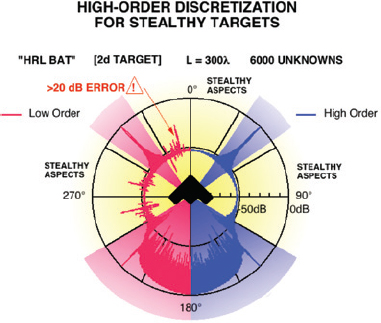
11 / Simulation of two-dimensional radar scattering from a stealthy airplane, similar in shape to the B-2 bomber. The front of the plane is at the top; two simulated radar signals are plotted in red and purple. On the left (red) is a computation using a low-order discretization. It incorrectly shows a considerable radar signal to the front and side of the airplane. On the right (purple) is a more accurate reconstruction of the radar signal, which would in practice be computed with the Fast Multipole Method. Note the near absence of a radar signal to the front and side of the airplane. (Actual three-dimensional data for the B-2 bomber are classified.) Reprinted with permission from Mark Stalzer, California Institute of Technology. /
computed quickly, using the multipole approximation. Because most of the calculation is accelerated and only a tiny part is slow, the overall effect is a great speedup.
In practice, the Fast Multipole Method has meant the difference between computing the radar signature of a coarse approximation to an airplane and computing the radar signature of a particular model of aircraft. While it would be tempting to say that it has saved the Air Force millions of dollars, it would be more accurate to say that it has enabled them to do something they could not previously do at any price (see Figure 11).
The applications of the Fast Multipole Method have not been limited to the military. In fact, its most important application from a business perspective is for the fabrication of computer chips and electronic components. Integrated circuits now pack 10 billion transistors into a few square centimeters, and this makes their electromagnetic behavior hard to predict. The electrons don’t just go through the wires they are supposed to, as they would in a normal-sized circuit. A charge in one wire can induce a parasitic charge in other wires that are only a few microns away.
Predicting the actual behavior of a chip means solving Maxwell’s equations, and the Fast Multipole Method has proved to be the perfect tool. For example, most cell phones now contain components that were tested with the Fast Multipole Method before they were ever manufactured.
At present the semiconductor companies use a slightly simpler version of the Fast Multipole Method than the original algorithm developed for Defense Advanced Research Projects Agency. The simpler version is applicable to static electric fields or
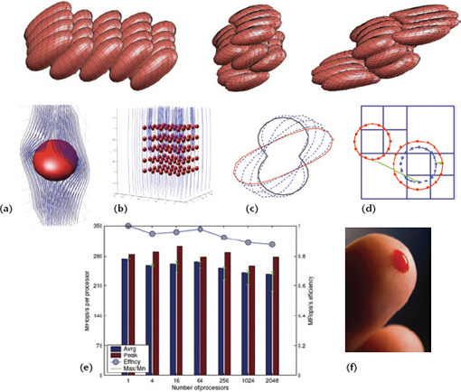
12 / A simulation of red blood cells, performed on the Jaguar computer at Oak Ridge National Laboratory, won the Gordon Bell Prize for best use of supercomputing in 2010. The Fast Multipole Method was used to accelerate the computation of long-range interactions between red blood cells and plasma. A single-cell computation is shown in (a) and multicell interactions are shown in (b). Each cell’s boundary is discretized (c). The hierarchical structure of the Fast Multipole Method computation is shown schematically in (d) and (e). The volume of blood simulated is shown in (f). This was 10,000 times the volume of any previous computer simulation of blood flow that accurately represented cellular interactions. Reprinted from A. Rahimian, I. Lashuk, S.K. Veerapaneni, C. Aparna, D. Malhotra, L. Moon, R. Sampath, A. Shringarpure, J. Vetter, R. Vuduc, D. Zorin, and G. Biros, 2010, Petascale direct numerical simulation of blood flow on 200K cores and heterogeneous architectures. ACM/IEEE Supercomputing (SCxy) Conference Series: 1-11, Figure 1 with permission from IEEE. /
low-frequency electromagnetic waves. Believe it or not, even a 1-gigahertz chip—which operates at 1 billion cycles per second—operates at low frequency from the point of view of the Fast Multipole Method! That is because a 1-GHz electromagnetic wave still has a wavelength that is much longer than the width of a chip.
However, it is quite possible that the computer industry will one day graduate to optical chips, which will use light waves instead of electricity to communicate. A wavelength of light is much shorter than the width of a chip. So for an integrated optical chip, the high-frequency version of the Fast Multipole Method will become an essential part of the product
development cycle. If so, the small investment in mathematical sciences that Auslander made in 1990 will pay off in an even bigger way three or four decades later.
Finally, it is worth noting that variants of the Fast Multipole Method are applicable to problems that have nothing to do with electromagnetism. The method is relevant to any situation where a large number of objects interact with one another, such as stars in a galaxy or red blood cells in an artery. Each red blood cell affects many nearby red blood cells, because they are packed quite densely inside a viscous fluid (the plasma). In addition, blood cells are squishy: they bend around curves or around each other. To take this into account, a good computer simulation needs to track dozens of points on the surface of each blood cell, and those points interact strongly with one another as the cell maintains its structural integrity.
In 2010, a simulation of blood flow based on the Fast Multipole Method won the prestigious Gordon Bell Prize for peak performance on a genuine (i.e., not a toy) problem of supercomputing (Figure 12). Researchers at the Georgia Institute of Technology and New York University used the Oak Ridge National Laboratory’s Jaguar supercomputer to simulate the flow of 260 million deformable red blood cells (about the number from one finger prick). This smashed the previous record of only 14,000 cells and allowed the simulation to approximate the real fluid properties of blood. Although media attention focused on the supercomputer, the calculation would not have been possible without the Fast Multipole Method, implemented in a new way that was adapted to parallel computing. Ultimately, such simulations will help doctors understand blood clotting better and perhaps improve anticoagulation therapy for people with heart disease.
The mathematical sciences underpin many of the technologies on which national defense depends. Cutting-edge mathematics and statistics lie behind smart sensors and advanced control and communications. They are used throughout the research, development, engineering, and test and evaluation process. They are embedded in simulation systems for planning and for warfighter training. Since World War II, the mathematical sciences have been key contributors to national defense, and their utility continues to expand. This graphic illustrates some of those impacts.
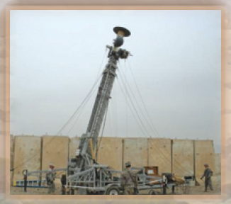
The mathematical sciences are used in planning logistics, deployments, and scenario evaluations for complex operations.
Mathematical simulations allow predictions of the spread of smoke and chemical and biological agents in urban terrain.
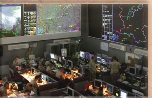
Mathematics and statistics underpin tools for control and communications in tactical operations.
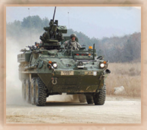
Mathematics is used to design advanced armor.
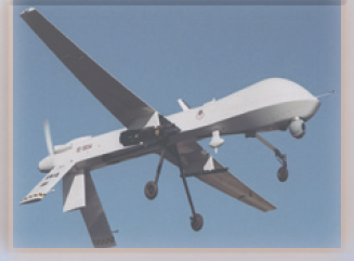
Signal analysis and control theory are essential for drones.
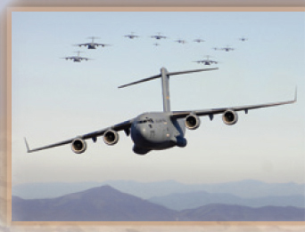
Large-scale computational codes are used to design aircraft, simulate flight paths, and train personnel.
Signal processing facilitates communication capabilities.
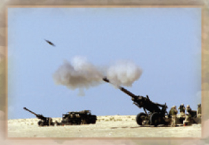
Satellite-guided weapons utilize GPS for highly-precise targeting, while mathematical methods improve ballistics.
Mobile translation systems employ voice recognition software to reduce language barriers when human linguists are not available More generally, math-based simulations are used in mission and specialty training.
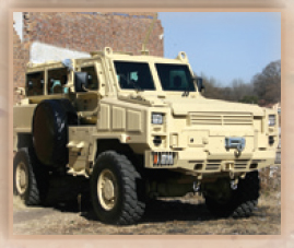
Modeling and simulation facilitates trade-off analysis during vehicle design, while statistics underpins test and evaluation.


