
Appendix B
Sea-Level Rise in the Northeast Pacific Ocean
Sea-level rise along the west coast of the United States can be estimated using tide gage records from coastal stations or satellite altimetry data from the northeast Pacific Ocean. Appendix A estimated sea-level rise along the coast by correcting tide gage records for total vertical land motions—including tectonics, glacial isostatic adjustment (GIA), and fluid withdrawal and recharge—using Global Positioning System data. This Appendix estimates sea-level rise using tide gage records corrected for the GIA component of vertical land motion, then compares the estimates with regional altimetry data, which are also corrected for GIA.
It is well established that sea-level rise varies geographically and that this geographical pattern can be measured using satellite altimetry. However, satellite altimetry records are short (< 20 years), and the estimated sea-level trend is significantly influenced by ocean variability at interannual or longer timescales. On the other hand, satellite altimetry is much less affected by GIA than tide gages, and it is unaffected by vertical land motions caused by tectonics or fluid extraction or recharge. This appendix examines the extent to which tide gages and satellite altimetry measure the same sea-level variations at the seasonal and interannual scales in the northeast Pacific. This analysis differs from previous studies, which compared satellite altimetry with island tide gage data for calibration and validation purposes (e.g., Chambers et al., 2003; Mitchum et al., 2010). Such studies show that sea-level trends determined from tide gages are similar to trends determined from altimetry measurements made near the tide gage station (averaged within 220–330 km), as long as the vertical motion of the tide gage benchmark is known. The analysis below compares records from 21 tide gages and altimetry data from the northeast Pacific Ocean over the same timespan, 1992–2008. This exercise is intended (1) to assess confidence in both types of sea-level measurements, (2) to provide an independent check on the GPS-corrected tide gage sea-level estimates presented in Appendix A, and (3) to possibly discern the source of vertical land motion at the tide gage benchmarks along the coasts of California, Oregon, and Washington.
CORRECTIONS
Sea-level data from the TOPEX/Poseidon, Jason-1, and Jason-2 altimeters were obtained for 1992–2010 from JPL PODAAC,1 and tide gage data were obtained from the Permanent Service for Mean Sea Level (PSMSL). To compare the tide gage and regional altimetry sea-level trends, the altimetry data were first corrected for instrument, media, and geophysical effects, and the gage data were corrected for atmosphere barotropic effects using the inverted barometer assumption. Both types of data were then corrected for the effect of GIA, assuming that GIA is the only geophysical process affecting motion of either the land or the seafloor, for tide gage or altimetry records, respectively. The corrections to the data and the conversion to geocentric sea-level trends are described below.
__________
1 See <http://podaac.jpl.nasa.gov>.
The sea-level data from TOPEX/Poseidon (ground tracks from the original mission and the tandem mission phase), Jason-1, and Jason-2 were processed by subtracting a mean sea surface from the corrected sea surface topography measurements, and applying cross-track and along-track gradient corrections. Relative altimeter biases between the three different altimeters were estimated globally with respect to TOPEX then applied to the regional study. The altimeter sea surface topography measurements were corrected for media (ionosphere, dry, and wet troposphere), instrument, and geophysical (solid Earth, pole and ocean tides, sea state bias, and atmosphere barotropic response) conditions.
The altimeter sea-level time series were corrected for dynamic atmosphere response using the AVISO dynamic atmosphere response model (Carrère and Lyard, 2003) and for atmospheric pressure (inverse barometer [IB]) using the European Centre for Medium-Range Weather Forecasts surface pressure model. These corrections were applied to the along-track sea-level data from each altimeter, and the data were averaged around each tide gage site into monthly measurements. The monthly tide gage sea-level data were corrected for IB effects using the National Oceanic and Atmospheric Administration Earth System Research Laboratory (NOAA ESRL) 20th Century Reanalysis V2 (Table B.1).2
Semiannual and annual signals for both the altimetry and tide gage sea-level time series were removed. Removal of these signals improved the correlation between the altimetry and tide gage sea-level data and reduced their root mean square (RMS) differences. Application of the atmosphere correction further reduced the sea-level variability of both the altimetry and tide gage data. The IB corrections had little impact on the linear sea-level trend estimated from the tide gage records, however they slightly reduced the correlation between the tide gage and altimetry sea-level data from 0.79 to 0.64 (Table B.1).
Both the tide gage and the altimetry sea-level data were corrected for GIA, and thus their estimated trends are directly comparable. For the tide gages, the sea-level trend was calculated by subtracting the GIA predicted relative sea-level trend from the tide gage estimated linear trend. The GIA predicted relative sea-level trend (absolute sea-level change minus the height change of the solid earth surface) at the gage benchmark is effectively a predicted vertical land motion estimate, with an opposite sign, if GIA is the only geophysical process. For altimetry, the geocentric sea-level trend was calculated by subtracting the GIA-model predicted absolute sea-level change from the altimeter sea-level trend (Peltier, 2001, Tamisiea, 2011). Table B.2 shows long-term tide gage estimated sea-level trends, corrected using the van der Wal GIA model, and the GIA model corrections from various GIA models.
RESULTS
Figure B.1 shows the GIA-model predicted relative sea-level change (computed by subtracting the crustal uplift from absolute sea-level change) from an ensemble of eight GIA models in western North America. Predicted values differ significantly from one another in Washington and Canada, but are similar along the coast. In the study region where the tide gages are located, the spread of GIA predicted values is between 1 mm yr-1 and 2 mm yr-1, mostly dominated by the difference in the predicted uplift rate of the solid earth.
Figure B.2 shows the tide gage estimated long-term sea-level trends, ~1900–2009, corrected for GIA using an ensemble of 17 models, as a function of latitude. The discrepancy in sea-level trend due to the choice of different GIA models is approximately 1 mm yr-1 for the southern tide gages and up to 2 mm yr-1 for the Washington gages (Figure B.2).
Figure B.3 compares the estimated sea-level trends for both tide gages and satellite altimetry for 1992–2008. Both records were corrected for IB and for GIA using the van der Wal GIA model (van der Wal et al., 2009). The sea-level trend determined from satellite altimetry (background color) and from the tide gages (color-coded circles) is in reasonable agreement along the coast. Figure B.3 shows that the sea-level trend is nonuniform geographically, and that satellite altimetry can measure the sea-level trends much further away from the coastal regions where tide gages reside.
__________
2 The National Centers for Environmental Prediction (NCEP) Reanalysis Derived Data (Kalnay et al., 1996), which is valid for 1948–2011 and has a spatial resolution of 2.5° × 2.5°, can also be used to correct for inverse barometer. Tests showed that the performance of both the NOAA ESRL and NCEP models was almost identical.
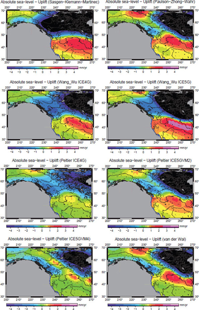
FIGURE B.1 Selected GIA model predicted relative sea-level rise (absolute sea-level change minus height change) in western North America. Tide gage locations are shown as blue dots. For the Paulson-Zhang-Wahr model, only the absolute sea level is available, so a theoretical predicted relationship between absolute sea-level change and uplift (Wahr et al., 1995) was used to compute the associated relative sea-level change.
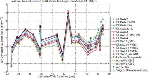
FIGURE B.2 Tide gage estimated long-term sea-level trends, corrected for GIA using an ensemble of 17 models at 21 locations from south (San Diego, 32.72°N) to north (Friday Harbor, 48 55°N).
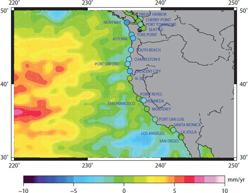
FIGURE B.3 Comparison of geocentric sea-level trends, in mm yr-1, for 1992–2008 from 21 tide gages along the coast of California, Oregon, and Washington (color-coded circles) and from TOPEX/Poseidon, Jason-1, and Jason-2 satellite altimetry missions (background colors).
TABLE B.1 Effect of Inverted Barometer Corrections on Estimated Sea-Level Trends in the Northeast Pacific Ocean
| Without IB Correction to Tide Gage or Altimetry Data | IB Correction Using NOAA ESRL 20th Century Reanalysis V2 Model | |
| Linear sea-level trend averaged from 21 tide gages, 1906–2008 | 0.71 ± 0.04 mm yr-1 | 0.76 ± 0.04 mm yr-1 |
| RMS difference of average sea level, altimetry minus tide gage, 1992–2008 | 3.3 cm | 3.3 cm |
| Correlation, 1992–2008 | 79.2% | 63.7% |
Figure B.4 compares the tide gage and altimetry sea-level time series for 1992–2008 at each tide gage site in the northeast Pacific study region. Note than the trend estimates for both data types are probably in error, primarily because of the short data spans and the large sea-level variability at interannual or longer timescales. RMS differences and correlations are given at the top of each figure, and the sea-level trends are indicated by the straight lines. The figures show that seasonal variations between the altimetry and tide gage sea-level time series are largely coherent (as indicated by RMS differences and correlations), indicating that the two independent sea-level measurement systems observed the same sea-level variations at seasonal and interannual timescales during 1992–2008. However, some estimated trends of individual tide gages are substantially different from the altimetry trend, likely because of the poor trend determination due to short data spans and/or because vertical land motion at some of these tide gage sites is dominated by non-GIA processes, such as tectonics.
Next, the estimated gage and altimetry trends were averaged to further examine whether these two independent types of data measure the same sea level at the same location. The top panel of Figure B.5 shows the averaged tide gage and altimetry sea-level time series for 1992–2008. The estimated trends are -2.0 ± 0.7 mm yr-1 for the tide gages and 0.0 ± 0.4 mm yr-1 for altimetry. Although these trend estimates are significantly different (because of short data spans and possibly non-GIA related uplift or subsidence at the tide gage benchmarks), both time series show good coherence at seasonal and interannual timescales. They have an averaged RMS difference of 3.2 cm and an averaged correlation of 65.9 percent, indicating that they measure essentially the same sea level. The bottom panel of Figure B.5 compares the short-term (last few decades) variation in sea level determined from tide gages and altimetry with the long-term (extending back to 1900) variation in sea level determined from tide gages. The stated reasons for the trend difference between altimetry and gage is further confirmed by the differences in the short-term (1992–2008) and long-term (1900–2009) gage trend estimates, at -2.0 ± 0.7 mm yr-1 and 0.76 ± 0.04 mm yr-1, respectively. The latter represents a more robust sea-level trend estimate over the study region.
The above analysis indicates that both altimetry and tide gage observed sea-level variations are coherent at seasonal and interannual timescales. The difference in trend estimates of ~2 mm yr-1 over the timespan (1992–2008), correcting for vertical motion assuming an ongoing GIA process, could be caused by the short data span or by non-GIA related vertical motion at some of tide gages in the study region.
REFERENCES
Carrère, L., and F. Lyard, 2003, Modelling the barotropic response of the global ocean to atmospheric wind and pressure forcing — Comparisons with observations, Geophysical Research Letters, 30, 1275.
Chambers, D., S.A. Hayes, J.C. Ries, and T. Urban, 2003, New TOPEX sea state bias models and their effect on global mean sea level, Journal of Geophysical Research, 108, 3305, doi:10.1029/2003JC001839.
Kalnay, E., M. Kanamitsu, R. Kistler, W. Collins, D. Deaven, L. Gandin, M. Iredell, S. Saha, G. White, J. Woollen, Y. Zhu, M. Chelliah, W. Ebisuzaki, W. Higgins, J. Janowiak, K.C. Mo, C. Ropelewski, J. Wang, A. Leetmaa, R. Reynolds, R. Jenne, and D. Joseph, 1996, The NCEP/NCAR 40-year reanalysis project, Bulletin of the American Meteorological Society, 77, 437-470.
Mitchum, G., R. Nerem, M. Merrifield, and W. Gehrels, 2010, Modern sea level estimates, in Understanding Sea-Level Rise and Variability, J. Church, P. Woodworth, T. Aarup, and W. Wilson, eds., Wiley-Blackwell, UK, pp. 122-428.
Paulson, A., S.J. Zhong, and J. Wahr, 2007, Inference of mantle viscosity from GRACE and relative sea level data, Geophysical Journal International, 171, 497-508.
TABLE B.2 Sea-Level Trends and Different GIA Corrections for 21 Tide Gages
| Tide Gage | van der Wala (mm yr-1) | Peltier ICE4G VM2 (mm yr-1) | ||||||
| Name | Latitude | Longitude | Period | Geocentric Sea-Level Trendb (mm yr-1) |
Absolute Sea-Level Trendc |
Relative Sea-Level Trendc |
Absolute Sea-Level Trend |
Relative Sea-Level Trend |
| Cherry Point | 48.867 | -122.750 | 1985–2009 | -0.03 | -0.23 | -0.50 | 0.05 | -1.10 |
| Friday Harbor | 48.550 | -123.000 | 1934–2009 | 1.13 | -0.25 | -0.17 | 0.03 | -0.83 |
| Neah Bay | 48.367 | -124.617 | 1934–2009 | -1.63 | -0.28 | 0.32 | 0.00 | -0.40 |
| Port Townsend | 48.117 | -122.750 | 1972–2009 | 1.48 | -0.26 | 0.12 | 0.01 | -0.53 |
| Seattle | 47.760 | -122.333 | 1899–2009 | 2.11 | -0.28 | 0.43 | -0.01 | -0.21 |
| Toke Point | 46.717 | -123.967 | 1973–2009 | 1.04 | -0.33 | 1.04 | -0.06 | 0.50 |
| Astoria | 46.217 | -123.767 | 1925–2009 | -0.29 | -0.35 | 1.07 | -0.07 | 0.64 |
| South Beach | 44.633 | -124.050 | 1967–2009 | 2.42 | -0.38 | 0.91 | -0.11 | 0.80 |
| Charleston II | 43.350 | -124.317 | 1970–2009 | 0.82 | -0.40 | 0.58 | -0.13 | 0.61 |
| Port Orford | 42.733 | -124.500 | 1985–2009 | 1.49 | -0.40 | 0.45 | -0.14 | 0.50 |
| Crescent City | 41.750 | -124.200 | 1933–2009 | -0.67 | -0.41 | 0.22 | -0.15 | 0.29 |
| North Spit | 40.767 | -124.217 | 1985–2009 | 4.39 | -0.41 | 0.13 | -0.16 | 0.20 |
| Point Reyes | 38.000 | -122.983 | 1975–2009 | 1.68 | -0.43 | 0.04 | -0.18 | 0.06 |
| San Francisco | 37.800 | -122.467 | 1854–2009 | 1.98 | -0.43 | -0.01 | -0.17 | 0.02 |
| Alameda | 37.767 | -122.300 | 1939–2009 | 0.81 | -0.43 | -0.03 | -0.17 | 0.01 |
| Monterey | 36.600 | -121.883 | 1973–2009 | 1.11 | -0.44 | 0.05 | -0.18 | 0.04 |
| Port San Luis | 35.167 | -120.750 | 1945–2009 | 0.78 | -0.45 | 0.08 | -0.19 | 0.05 |
| Santa Monica | 34.017 | -118.500 | 1933–2009 | 1.44 | -0.45 | 0.01 | -0.19 | 0.00 |
| Los Angeles | 33.717 | -118.267 | 1923–2009 | 0.83 | -0.45 | 0.03 | -0.19 | 0.01 |
| La Jolla | 32.867 | -117.250 | 1924–2009 | 2.06 | -0.45 | 0.05 | -0.19 | 0.03 |
| San Diego | 32.717 | -117.167 | 1906–2009 | 2.09 | -0.45 | 0.06 | -0.19 | 0.03 |
| Average | 1.19 | -0.38 | 0.23 | -0.11 | 0.03 | |||
SOURCE: ICE4G VM2 (Peltier, 2002), ICE5G VM2, and ICE5G VM4 (Peltier, 2004) models are from <http://www.sbl.statkart.no/projects/pgs/authors>.
ICE5G predictions were computed by R. Peltier (personal communication, 2011). GIA model results (Wang and Wu, 2006; Paulson et al., 2007; van der Wal et al., 2009; Sasgen et al., 2012; H. Wang, personal communication, 2011) were provided by the respective authors.
a Model includes rotational feedback.
b Tide gage geocentric sea-level trend = tide gage relative sea-level trend minus GIA predicted relative sea-level trend. The van der Wal model was used for the GIA correction. Tide gage relative sea-level trend was estimated by fitting a trend simultaneously with terms modeling semiannual and annual variations.
c GIA predicted relative sea-level trend = absolute sea-level change minus height change of the solid earth surface.
Peltier, W., 2001, Global glacial isostatic adjustment and modern instrumental records of relative sea level history, in Sea Level Rise: History and Consequences, B. Douglas, M. Kearney, and S. Leatherman, eds., International Geophysics Series, 75, Academic Press, pp. 65-95.
Peltier, W.R., 2002, On eustatic sea level history: Last Glacial Maximum to Holocene, Quaternary Science Reviews, 21, 377-396.
Peltier, W., 2004, Global glacial isostasy and the surface of the ice-age Earth: The ICE-5G (VM2) model and GRACE, Annual Review of Earth and Planetary Sciences, 32, 111-149.
Sasgen, I., V. Klemann, and Z. Martinec, 2012, Towards the joint inversion of GRACE gravity fields for present-day ice-mass changes and glacial-isostatic adjustment in North America and Greenland, Journal of Geodynamics, in press.
Tamisiea, M., 2011, Ongoing glacial isostatic contributions to observations of sea level change, Geophysical Journal International, 186, 1036-1044.
van der Wal, W., A. Braun, P. Wu, and M. Sideris, 2009, Prediction of decadal slope changes in Canada by glacial isostatic adjustment modeling, Canadian Journal of Earth Sciences, 46, 587-595.
Wahr, J.M., D. Han, and A. Trupin, 1995, Predictions of vertical uplift caused by changing polar ice volumes on a viscoelastic Earth, Geophysical Research Letters, 22, 977-980.
Wang, H., and P. Wu, 2006, Effects of lateral variations in lithospheric thickness and mantle viscosity on glacially induced surface motion on a spherical, self-gravitating Maxwell Earth, Earth and Planetary Science Letters, 244, 576-589.
| Peltier ICE5G VM2a (mm yr-1) | Peltier ICE5G VM4a (mm yr-1) | Wang-Wu ICE4G (mm yr-1) | Wang-Wu ICE5G (mm yr-1) | Sasgen-Klemann- Martinec (mm yr-1) | |||||
| Absolute Sea-Level Trend |
Relative Sea-Level Trend |
Absolute Sea-Level Trend |
Relative Sea-Level Trend |
Absolute Sea-Level Trend |
Relative Sea-Level Trend |
Absolute Sea-Level Trend |
Relative Sea-Level Trend |
Absolute Sea-Level Trend |
Relative Sea-Level Trend |
| -0.91 | 0.23 | -0.81 | -0.42 | 0.25 | -1.12 | 0.37 | 0.22 | 0.08 | -0.23 |
| -0.93 | 0.61 | -0.83 | -0.09 | 0.22 | -0.84 | 0.33 | 0.42 | 0.03 | -0.22 |
| -0.96 | 1.18 | -0.85 | 0.40 | 0.18 | -0.45 | 0.26 | 0.63 | -0.04 | 0.04 |
| -0.96 | 0.88 | -0.85 | 0.14 | 0.20 | -0.60 | 0.31 | 0.61 | -0.01 | -0.06 |
| -0.99 | 1.16 | -0.87 | 0.37 | 0.18 | -0.32 | 0.28 | 0.82 | -0.06 | 0.09 |
| -1.04 | 1.82 | -0.91 | 0.90 | 0.11 | 0.19 | 0.17 | 1.19 | -0.16 | 0.60 |
| -1.06 | 1.79 | -0.92 | 0.85 | 0.09 | 0.32 | 0.15 | 1.27 | -0.17 | 0.59 |
| -1.09 | 1.53 | -0.95 | 0.52 | 0.03 | 0.59 | 0.06 | 1.44 | -0.19 | 0.80 |
| -1.10 | 1.23 | -0.96 | 0.24 | -0.01 | 0.65 | -0.01 | 1.44 | -0.18 | 0.72 |
| -1.11 | 1.15 | -0.96 | 0.17 | -0.03 | 0.67 | -0.03 | 1.44 | -0.18 | 0.72 |
| -1.11 | 0.95 | -0.96 | 0.03 | -0.05 | 0.62 | -0.06 | 1.34 | -0.16 | 0.60 |
| -1.12 | 0.90 | -0.97 | 0.04 | -0.07 | 0.60 | -0.09 | 1.28 | -0.15 | 0.66 |
| -1.13 | 0.76 | -1.00 | 0.10 | -0.10 | 0.49 | -0.14 | 1.06 | -0.12 | 0.47 |
| -1.13 | 0.69 | -1.00 | 0.05 | -0.10 | 0.45 | -0.14 | 1.01 | -0.12 | 0.35 |
| -1.13 | 0.67 | -1.00 | 0.03 | -0.10 | 0.44 | -0.14 | 0.99 | -0.12 | 0.30 |
| -1.14 | 0.68 | -1.01 | 0.12 | -0.11 | 0.43 | -0.15 | 0.96 | -0.11 | 0.41 |
| -1.14 | 0.61 | -1.02 | 0.13 | -0.12 | 0.40 | -0.17 | 0.87 | -0.10 | 0.40 |
| -1.14 | 0.45 | -1.03 | 0.04 | -0.11 | 0.31 | -0.17 | 0.75 | -0.09 | 0.26 |
| -1.14 | 0.45 | -1.03 | 0.06 | -0.12 | 0.31 | -0.17 | 0.75 | -0.08 | 0.32 |
| -1.14 | 0.44 | -1.03 | 0.09 | -0.12 | 0.27 | -0.17 | 0.70 | -0.08 | 0.29 |
| -1.14 | 0.44 | -1.03 | 0.10 | -0.12 | 0.27 | -0.17 | 0.69 | -0.08 | 0.29 |
| -1.08 | 0.89 | -0.95 | 0.19 | 0.01 | 0.18 | 0.02 | 0.95 | -0.10 | 0.35 |
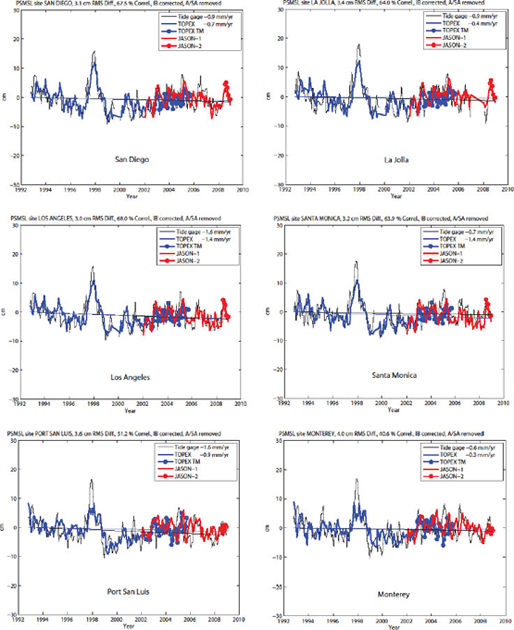
FIGURE B.4 Comparisons for 1992–2008 between the sea-level time series for 21 tide gages and averaged altimetry (TOPEX, Jason-1, and Jason-2) in the northeast Pacific study region.
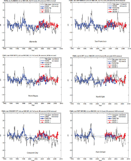
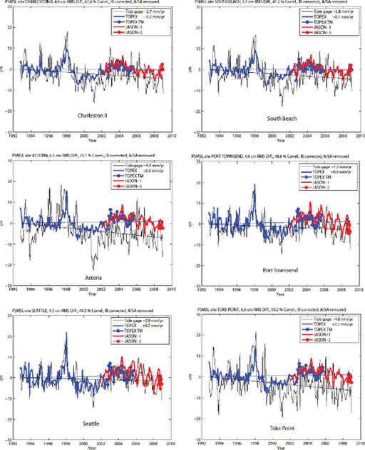
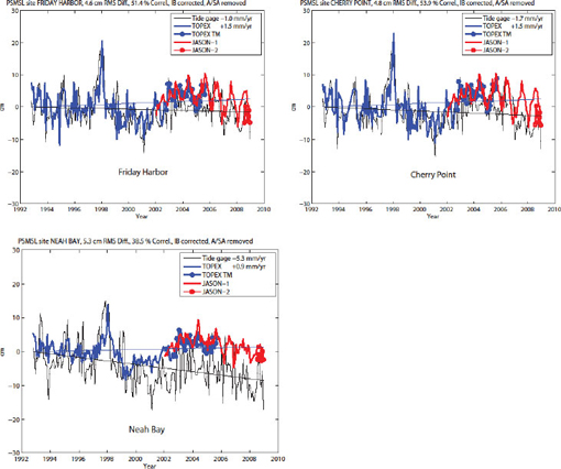
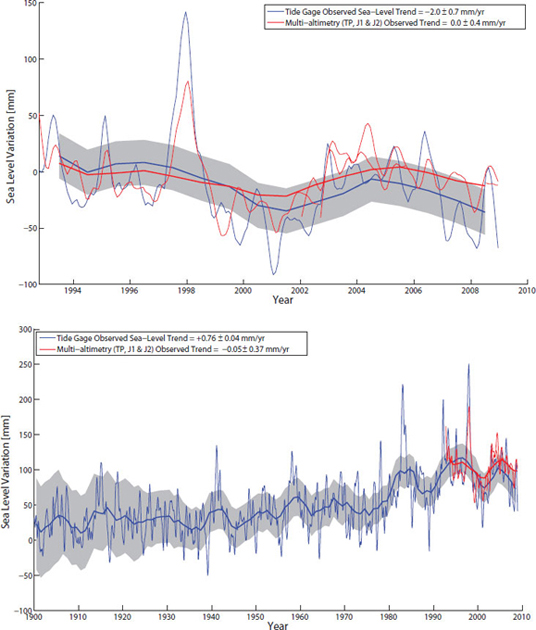
FIGURE B.5 Averaged tide gage and altimetry sea-level time series for 1992–2008 (top), and the averaged tide gage time series for 1900–2008 shown also with altimetry sea-level time series (bottom). Inverted barometer and GIA corrections have been applied to both tide gage and altimetry sea-level records. The bottom panel also shows yearly averages, solid blue and red lines for tide gage and altimetry sea level, respectively, and estimated tide gage sea-level uncertainty in gray shades.


