
5
Projections of Sea-Level Change
Observations provide unequivocal evidence that global mean sea level has been rising over the past century, but that the rate of sea-level rise has significant regional variability. The key question for planners is how much sea level will rise in their region in an increasingly warm future world. Most projections are based on knowledge of the current contributions to sea-level change and assumptions about future warming and the behavior of key geophysical processes. This chapter describes methods for projecting global and regional sea-level rise, summarizes recent results, and presents the committee’s own projections for the years 2030, 2050, and 2100, relative to year 2000. The chapter begins with a discussion of the global projections, then describes how these are adjusted using local and regional information from the U.S. west coast to develop projections for California, Oregon, and Washington. The chapter concludes with a discussion of rare extreme events that could induce a large, rapid change in sea level along the west coast of the United States.
RECENT GLOBAL SEA-LEVEL PROJECTIONS
Projections of future global sea-level change are commonly made using models of the primary processes that contribute to global sea-level change—the transfer of fresh water from the melting cryosphere to the oceans, and changes in water density (steric changes) arising mainly from the thermal expansion of ocean water as it warms. Although the steric contribution can be computed from ocean models, the cryospheric contribution cannot yet be modeled satisfactorily. Given this shortcoming, some investigators use current observations to extrapolate the future behavior of the cryosphere. Another approach to projections, called the “semi-empirical” approach, is based on the observed relationship between sea-level change and global temperature change, and takes no account of the individual contributions to sea-level rise or their physical constraints. Recent projections of global sea-level rise from these different approaches are summarized below.
Models of Physical Processes
The Intergovernmental Panel on Climate Change (IPCC) Fourth Assessment Report projected global sea-level rise to 2100, relative to the year 2000, using numerical models forced by different emission scenarios, as well as simplified climate models. The scenarios represent a range of driving forces and emissions developed using different assumptions about demographic, social, economic, technological, and environmental developments (Box 5.1). The IPCC (2007) projected the individual contributions of steric changes and melting of glaciers and ice caps, the Greenland Ice Sheet, and the Antarctic Ice Sheet to future sea-level change for each emission scenario, then summed the contributions. Changes in water stored in other land reservoirs or extracted from the ground or aquifers were considered too uncertain to project. The IPCC (2007) projections are given in Table 5.1 and are discussed below.
BOX 5.1
IPCC (2000) Emission Scenarios
The IPCC Fourth Assessment Report projected global sea levels over the next 100 years based on 6 families of emission scenarios described in IPCC (2000). The A1 scenario family assumes high economic growth, low population growth that peaks mid century, and the rapid introduction of more efficient technologies. Within this family are scenarios designated as A1FI (fossil fuel intensive), A1B (balanced fuel), and A1T (predominantly nonfossil fuels). The A2 scenario family assumes slower economic growth and technological change, but high population growth. The B1 scenario family assumes the same low population growth as the A1 scenarios, but a shift toward a lower-emission service and information economy and cleaner technologies. Finally, the B2 scenario family assumes moderate population growth, intermediate economic growth, and slower and more diverse technological change than in the B1 and A1 scenarios. The A1FI scenario yields the highest carbon dioxide (CO2) emissions by 2100, and the B1 scenario yields the lowest CO2 emissions.
TABLE 5.1 IPCC (2007) Projected Contributions to Global Sea-Level Change, Relative to 2000
| Projections for 2100 (cm) | ||||||
| Term | B1 | B2 | MB | A1T | A2 | A1FI |
| Thermal expansion | 10–24 | 12–28 | 13–32 | 12–30 | 14–35 | 17–41 |
| Glaciers and ice caps | 7–14 | 7–15 | 8–15 | 8–15 | 8–16 | 8–17 |
| Greenland Ice Sheet SMB | 1–5 | 1–6 | 1–8 | 1–7 | 1–8 | 2–12 |
| Antarctica Ice Sheet SMB | -10–-2 | -11–-2 | -12–-2 | -12–-2 | -12–-3 | -14–-3 |
| Sea-level rise | 18–38 | 20–43 | 21–48 | 20–45 | 23–51 | 26–59 |
| Scaled-up ice sheet discharge | 0–9 | 0–11 | -1–13 | -1–13 | -1–13 | -1–17 |
SOURCE: Adapted from Table 10.7 in Meehl et al. (2007).
NOTE: SMB = surface mass balance.
Steric Contributions
The IPCC Fourth Assessment Report used general circulation models (GCMs) of the ocean and atmosphere to estimate global steric response. Because the GCM simulations were only available for three emission scenarios, simplified climate models were used for the other three scenarios. Global ocean models compute both temperature and salinity, so their outputs can be used directly to calculate changes in sea level due to thermal expansion (thermosteric changes) and changes in salinity (halosteric changes). Thermosteric contributions from the ocean general circulation models used in the IPCC Fourth Assessment Report are shown in Figure 5.1 (Meehl et al., 2007). Note that the model results vary with time and emission scenario. The IPCC (2007) projected that thermal expansion would account for 55–69 percent of sea-level rise in 2100 (Table 5.1).
Cryospheric Contributions
The IPCC (2007) estimated the cryosphere response using models of ice sheet surface mass balance in Greenland and Antarctica and empirical models of the mass balance response of glaciers and ice caps to temperature and precipitation forcing. They projected that glaciers and ice caps would be the largest source of new water to the oceans throughout the 21st century (Table 5.1). The ice sheets were projected to contribute less new water than glaciers and ice caps, mainly because the Antarctic contribution was expected to be negative (i.e., mass gained because of increased snowfall would withdraw water from the ocean). However, recent observations of Antarctica show the opposite—a growing Antarctic contribution to sea-level rise due to the rapid transfer of ice from land to the ocean by glacier flow and iceberg calving, referred to here as “rapid dynamic response” (see “Glaciers, Ice Caps, and Ice Sheets” in Chapter 3).
At the time data were synthesized for the IPCC Fourth Assessment Report (until mid-2006), rapid transfers of ice at a global level were only beginning to be observed. In addition, the relatively simple treatment of land ice dynamics in the climate models precluded simulation of rapid dynamics. Although stand-alone
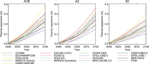
FIGURE 5.1 Thermal expansion contribution to global sea-level rise calculated by a range of models for three emission scenarios: A1B, A2, and B1. SOURCE: Figure 10.31 from Meehl et al. (2007).
ice sheet models with far more sophisticated dynamic capabilities have long been in use, they are difficult to drive in a realistic fashion with only climatic forcing variables, and are still not a feature of integrated atmosphere-ice-ocean models. Consequently, the IPCC (2007) treated ice sheets as fixed geographic features that could gain and lose mass through accumulation and ablation, but would not otherwise change size or undergo variations in flow. The IPCC (2007) attempted to account for rapid transfers of ice from land to ocean by scaling up certain components of the modeled results, shown in Table 5.1 under “Scaled-up ice sheet discharge.” However, the estimates were not based on physical models of ice sheet processes, and they were not included in the projections of global sea-level rise. The IPCC (2007) projections of the cryospheric contribution to sea-level rise are widely regarded as too low (e.g., Kerr, 2007; Pfeffer et al., 2008; van der Veen and IMASS, 2010; AMAP, 2011; Price et al., 2011).
Extrapolation of Land Ice Contributions
As noted above, some aspects of the cryospheric system are not yet understood well enough to be confidently represented in physical models, and many of the observations needed to characterize boundary and initial conditions or other model parameters are not available. Consequently, some investigators use extrapolation methods to project the cryospheric contribution to sea-level rise. Extrapolations carry past and present-day observed rates of change forward in time at rates that remain constant or vary according to assumed rules.
A number of recent studies have projected the future contributions of land ice to sea-level change by extrapolating observed trends in ice loss rates. Meier et al. (2007) extrapolated loss rates for the Greenland and Antarctic ice sheets and for aggregate glaciers and ice caps, and estimated that land ice would contribute ca. 8–16 cm to sea-level rise by 2050 and 17–56 cm by 2100 under plausible future conditions. The lower estimate assumed that present-day loss rates continued unchanged in the future. The higher estimate assumed that the present-day loss rate continued to increase in the future. Future sea-level rise could be less than the lower estimate only if global loss rates actually decreased in the future, an unlikely outcome of most climate and mass balance and ice dynamics modeling. Whether the higher estimate, which was not proposed as a firm upper limit, bounds the true upper range of outcomes is uncertain.
Pfeffer et al. (2008) made extrapolations that were intended to constrain the upper limits of glacier
and ice sheet contributions to sea level. Rather than project present-day observed rates forward in time, the authors calculated what loss rates would be required to achieve certain hypothesized future sea-level values. For example, a hypothesized 2 m rise in global sea level by 2100 from the Greenland Ice Sheet alone would require the average velocity of Greenland’s outlet glaciers to immediately rise to 49 km yr-1, which is highly unlikely and thus not a plausible future scenario. The authors also hypothesized a range of accelerated but reasonable glacier dynamic behavior for the Greenland and Antarctic ice sheets and for glaciers and ice caps, and they projected land ice contributions ranging from 0.8 m to 1.7 m by 2100, with roughly equal contributions from Greenland, Antarctica, and glaciers and ice caps.
Using comprehensive data extending back to 1992, Rignot et al. (2011a) constructed detailed mass loss time series for both the Greenland and Antarctic ice sheets, and extrapolated linear trends fit to that data to estimate future sea-level contributions from the ice sheets. The observed mass loss trends for 1992–2009 were 21.9 ± 1 GT yr-2 for the Greenland Ice Sheet and 14.5 ± 2 GT yr-2 for the Antarctica Ice Sheet. Extrapolating these loss trends forward to 2100, Rignot et al. (2011a) estimated a sea-level contribution from the ice sheets of 15 ± 2 cm by 2050 and 56 cm (with no stated uncertainty) by 2100. To arrive at a total land ice projection, Rignot et al. (2011a) used the glacier and ice cap values calculated by Meier et al. (2007). The uncertainty attached to the projection reflected the quality of fit of the linear regression of the trend to the loss rate data, rather than uncertainty of the data. The authors suggested that their calculations provide an indication of the potential contributions of ice sheets to sea level in the next century, but should not be regarded as projections, given the uncertainty in future acceleration of ice mass loss and the simplicity of their model.
The extrapolation methods used by Meier et al. (2007) and Rignot et al. (2011a) assume geostatistical stationarity—that the statistical characteristics during the period of observation remain valid over the period of extrapolation. For unvarying processes or for short extrapolation periods relative to the observation period, this assumption is justifiable. For time-varying processes or for long extrapolation periods, this assumption is more questionable. Glaciers, ice caps, and ice sheets may undergo changes in the next century that are quite unlike the changes recorded over the past few decades, such as an increase or decrease in the speed of marine-ending outlet glaciers. Analyses to evaluate the effects of non-stationarity (time-varying processes) and to qualitatively estimate the timescale for which extrapolations are valid are described in the committee’s projections of global sea-level rise (see “Cryosphere Contributions” below).
Semi-Empirical Models
Projections of 21st century sea-level rise are subject to uncertainties arising from the nonlinear responses of the Greenland and Western Antarctic ice sheets (Pfeffer et al., 2008; Rahmstorf, 2010), steric changes (Domingues et al., 2008; Leuliette and Miller, 2009), and contributions from mountain glaciers (Meier et al., 2007). One way to avoid the difficulties of accurately estimating these individual contributions is to postulate a simple link between observed sea-level rise and observed global temperature changes in the past (Rahmstorf, 2010). Such semi-empirical models are based on the simple physical concept that sea level rises faster as the Earth gets warmer. This concept is supported by observations on long timescales.
Early semi-empirical models assumed a linear relationship between global temperature and sea-level rise (e.g., Gornitz and Lebedeff, 1987), but subsequent refinements have included corrections for the time-response characteristics of sea level to temperature forcing. A frequently cited semi-empirical model to project future sea-level rise was developed by Rahmstorf (2007), who related rising sea level to global near-surface air temperature as follows:
dH/dt = a (T(t) - T0),
where H is the sea level, T is the mean global temperature, T0 is the baseline temperature at which sea level is stable, and a is the sea-level sensitivity, which measures how much the rate of sea-level rise accelerates per unit change in global temperature. The model postulates that if the temperature rises above T0, sea level will rise indefinitely at a rate determined by the magnitude of the temperature rise, so a linear rise in temperature with time leads to a quadratic change in sea level. The
unknown parameters a and T0 are determined from global sea-level reconstructions (e.g., Church and White, 2006) and global temperature data archived by the National Aeronautics and Space Administration Goddard Institute for Space Studies. Rahmstorf (2007) found that the parameter a is 3.4 mm yr-1/°C. Projecting the equation forward using the IPCC (2000) scenarios for temperature change yielded a rise in sea level between 0.38 m and 1.2 m by 2100.
A subsequent revision to the model (Vermeer and Rahmstorf, 2009) included an extra term b to allow sea level to respond directly to temperature change:
dS/dt = a (T -T0) + b dT/dt.
To gain confidence in the model, the authors calibrated the a and b coefficients with temperature data from 1880 to 2000, then verified the model over a 1,000-year time frame using sea-level proxy data for the past millennium. With this model and the IPCC (2000) emission scenarios, Vermeer and Rahmstorf (2009) projected that sea level would rise between 0.81 m and 1.79 m by 2100. Their projections for three of the IPCC (2000) emission scenarios are shown in Figure 5.2.
Grinsted et al. (2009) used a much longer temperature record and a different semi-empirical model to project sea-level rise:
dS/dt = (Seq - S)/τ,
where τ is the response time on the order of centuries, Seq is the equilibrium sea level at a fixed global temperature, and S is the global mean sea level relative to the mean over a well-documented time interval. Seq is assumed to change linearly with temperature. As the atmospheric temperature rises, the sea level rises at a rate that depends both on the magnitude of the total warming (which determines Seq - S) and the response time τ. Grinsted et al. (2009) calibrated their equation using several historical global temperature data sets, then used the IPCC (2000) scenarios to project into the future. For all IPCC (2000) emission scenarios, they projected that sea level would rise between 0.21 m and 2.15 m by 2100.
All of the semi-empirical model projections are higher than the IPCC (2007) projections by a factor of two or even three (Rahmstorf, 2010; Figure 5.2). The two projection approaches rest on different foundations—GCMs on the physical processes that
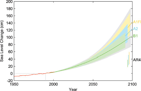
FIGURE 5.2 Projections of sea-level rise from 1990 to 2100, based on the Vermeer and Rahmstorf (2009) semi-empirical model and three IPCC (2000) emission scenarios (A1FI, A2, and B1). Uncertainty ranges are 1 standard deviation from the model means, and the gray shading is an added ± 7 percent, representing uncertainty in the fit of the data. The corresponding sea-level projections by IPCC (2007; labeled AR4) are shown for comparison in the bars on the bottom right. Also shown are the observations of annual global sea level (red line). SOURCE: Vermeer and Rahmstorf (2009).
cause sea level to rise and semi-empirical models on the observed relationship between temperature and sea level—so it is not surprising that they do not agree. Moreover, the IPCC (2007) projections are likely underestimates because they do not account fully for cryospheric processes. The highest projections made by semi-empirical models (more than 2 m of sea-level rise) are likely overestimates because they would require unrealistically rapid acceleration of glaciological processes (Pfeffer et al., 2008).
An advantage of semi-empirical models is that, by parameter fitting, they reproduce the observed past sea-level rise. However, the simple empirical connection found for the past may not hold in the future. In particular, the ice sheets appear to have been negligible sea-level contributors during the observational periods used by Gornitz and Lebedeff (1987), Rahmstorf (2007), and Vermeer and Rahmstorf (2009), but ice sheet dynamic response is widely regarded as the most uncertain aspect of sea-level change. Indeed, some events, such as ice shelf melting triggering an instability of the West Antarctic Ice Sheet, would not be factored into semi-empirical models.
COMMITTEE PROJECTIONS OF GLOBAL SEA-LEVEL RISE
The committee was charged with projecting both the individual contributions to global sea-level rise (e.g., thermal expansion, melting of land ice) and the total global sea-level rise for the years 2030, 2050, and 2100 (Task 1, see Box 1.1). Given the state of knowledge and the limited time and computational capability available for a National Research Council study, the committee chose a combination of approaches for its projections. The output of GCMs was used to project the steric contribution (primarily thermal expansion) to global sea-level rise over the three time frames. For the land ice projections, the committee extrapolated mass balance estimates. Like the IPCC (2007), the committee did not project land hydrology contributions because uncertainties are too large, and a recent comprehensive assessment (Milly et al., 2010) found that the primary sources (groundwater depletion) and sinks (reservoir storage) appear to effectively cancel out. The individual components were then summed and compared with results from semi-empirical methods. The projections are for individual years (2030, 2050, and 2100, relative to 2000), and were derived using single-year values from low-order curves, except for the steric values, as explained below. The projections are given in Table 5.2 and discussed below.
Steric Contribution
The most recent GCM results for the steric contribution that were available to the committee were from the Coupled Model Intercomparison Project Phase 3 (CMIP3), which were used in the IPCC Fourth Assessment Report. Although outputs from a new generation of GCMs are beginning to be available, performing computations of derived quantities like global sea-level changes from these new outputs is beyond the charge and capability of the committee. Consequently, the committee drew on the work of Pardaens et al. (2010), who analyzed an ensemble of IPCC (2007) model projections using the A1B emission scenario (Figure 5.3). Drs. Pardaens and Gregory1 provided the gridded annual mean sea-level data used in their paper, and the committee analyzed the combine steric and ocean dynamic height data for the globe.
The models in Pardaens et al. (2010) yielded time series of annual mean sea level spanning roughly the 21st century: the first year in the various model simulations ranged from 2000 to 2004, and the final year was 2099. The committee performed a quadratic fit on each model’s time series at each grid point and, using the values on the quadratic curves, obtained steric sea-level changes for 2030, 2050, and 2100 relative to year 2000 for each model. The results are presented in the first row of Table 5.2.
Uncertainties
The committee endeavored to incorporate and describe as accurately as possible the known sources of uncertainty in the steric projections. These uncertainties are related to future greenhouse gas and aerosol emissions and concentrations (human forcing), the response of global temperatures to human forcing, and the response of the ocean to those global temperature distributions. The IPCC (2007) treated uncertainty in
__________
1 See <http://www.met.rdg.ac.uk/~jonathan/data/ar4_sealevel/>.
TABLE 5.2 Committee’s Global Sea-Level Rise Projections (in cm) Relative to Year 2000
| 2030 | 2050 | 2100 | ||||
| Term | Projection | Range | Projection | Range | Projection | Range |
| Sterica | 5.4 ± 1.6 | 1.7–11.0 (B1–A1FI) |
9.9 ± 2.4 | 4.0–18.9 (B1–A1FI) |
24.2 ± 5.9 | 9.6–46.2 (B1–A1FI) |
| Glaciers and ice capsb | 2.9 ± 0.1 | 2.7–3.6 | 5.5 ± 0.2 | 5.1–7.3 | 14.3 ± 0.7 | 12.9–19.4 |
| Greenlandb | 2.3 ± 0.2 | 1.8–4.0 | 5.6 ± 0.7 | 4.3–10.2 | 20.1 ± 2.7 | 14.8–33.8 |
| Antarcticab | 2.9 ± 0.7 | 1.5–5.1 | 7.0 ± 2.1 | 3.0–13.3 | 24.0 ± 8.3 | 7.7–46.2 |
| Total Cryosphereb | 8.1 ± 0.8 | 6.6–12.2 | 18.0 ± 2.2 | 13.7–29.4 | 58.4 ± 8.8 | 40.9–94.1 |
| Sumc | 13.5 ± 1.8 | 8.3–23.2 | 28.0 ± 3.2 | 17.6–48.2 | 82.7 ± 10.6 | 50.4–140.2 |
| Semi-empiricald | 18 | 14–22 (Bl-AlFI) |
37 | 28–47 (B1-A1F1) |
121 | 78–175 (Bl-AlFI) |
a For the steric contribution, the projection is for scenario A1B from Pardaens et al. (2010), ±1 standard deviation computed for 20-year windows across models, and the range was determined by scaling the A1B projections for 2100 to the low value of B1 and the high value of A1FI for A1B, from Table 5.1.
b The cryospheric projection is an extrapolation from observed changes, ±1 standard deviation. The range column includes an additional dynamic contribution, described in Appendix E, which is used only for the high-end estimates.
c The low value of the range for each year (2030, 2050, 2100) was computed by subtracting twice the standard deviation from the mean in the projection column, and adjusting to the difference between A1B and B1. The high value of the range was computed by adding twice the standard deviation to the mean, adjusting to the difference between A1FI and A1B, and adding the dynamical imbalance contribution.
d Data from Vermeer and Rahmstorf (2009).
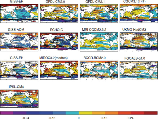
FIGURE 5.3 Combined static and wind-driven sea-level changes (1980-1999 to 2080-2099,units in m) for the indicated models, relative to each model’s global mean. The overlying contour lines are of the sea-level distribution in the baselne control simulations, averaged over a 120-year period (contours are every 0.2m).SOURCE: Pardaens et al. (2010).
human forcing by calculating results for six emission scenarios (Box 5.1, Table 5.1). The most common approach for treating uncertainty in the global temperature response is to use the results of many climate models, which also provides a range of projected values for the global ocean response. The IPCC (2007) global model simulations for the thermal expansion and dynamical components are available for only the B1, A1B, and A2 emission scenarios, and Pardaens et al. (2010) performed their calculations for only the A1B scenario. To provide a range of projections for all six scenarios, the committee used the ratios of thermal expansion projections from Table 5.1. For example, the global projection for the low value of B1 in 2030 was computed from the digital values in Pardaens et al. (2010) using the quadratic fit for 2030 as described above. To determine the range, this value was multiplied by the ratio of the low value of the thermal expansion term in 2100 for B1 to the low value for A1B (0.10/0.13). This approach slightly underestimates the B1 values for 2030 and 2050 because sea-level change under the B1 scenario is fairly linear (see Figure 5.1), but the difference is estimated to be within rounding error (a few mm).
Cryosphere Contribution
The committee projected the cryosphere contribution to global sea-level rise using adaptations of the Meier et al. (2007) extrapolation techniques and the Pfeffer et al. (2008) methods for evaluating uncertainty and establishing projection boundaries. The committee’s extrapolations were based on selected observational data for glaciers, ice caps, and the Greenland and Antarctic ice sheets. The most comprehensive time series of mass loss of the Greenland and Antarctic ice sheets is the Rignot et al. (2011a) compilation, which combines modeled surface mass balance and measured and modeled ice discharge to produce net balances for both ice sheets for 1992–2010, the earliest date from which continuous observations are available. For glaciers and ice caps, the committee used data from Dyurgerov and Meier (2005), Cogley (2009), and Dyurgerov (2010). At the time this report was being written, Dyurgerov and Meier’s (2005) mass balance data from glaciers and ice caps for the 1960–2005 period were the most recent global compilation of continuous records. Dyurgerov and Meier (2005) used known area and area-altitude distributions by region to scale up limited point mass balance observations. Their analysis considered surface mass balance changes directly modulated by climate and excluded losses by calving. Dyurgerov (2010) reevaluated the data used in Dyurgerov and Meier (2005) and made significant corrections to changing glacier areas during the period of observations. Cogley (2009) presented an independent data set, evaluated in 5-year increments from ca. 1850 to 2009, that includes both climatically forced and calving losses. The data for glaciers and ice caps were averaged using techniques that weight the data according to its quality as measured by the magnitude of the stated uncertainty (see Appendix E for details).
The base-rate extrapolation assumes that present-day observed trends in loss rates continue in the future. To investigate the effect of varying rapid dynamic discharge on these projections, the committee performed model experiments to calculate the effects of both acceleration and deceleration in ice discharge relative to observed present-day rates. Both possibilities have been examined in the literature. For example, Pfeffer et al. (2008) discussed the consequences of large-scale losses from both Greenland and Antarctica in hypothetical terms, and Rignot et al. (2011a) projected a large dynamic contribution to sea-level rise from the ice sheets on the basis of past observations. On the other hand, observations in Greenland (e.g., Moon et al., 2012) show that recently active outlet glaciers are slowing down, suggesting that rapid dynamics may have an episodic or periodic nature and that future increases in sea level from rapid dynamics may not be as dramatic as have been postulated elsewhere. Price et al. (2011) used a high-order numerical model to explore the effect of outlet glacier dynamics, their influence on upstream ice dynamics, and time variations in outlet glacier dynamics on future losses from the Greenland Ice Sheet.
Increased ice discharge beyond presently observed rates was simulated by extrapolating a multiple of present-day observed discharge forward in time to 2100 (see Appendix E). For glaciers and ice caps, an increment of flux equal to 50 percent of the present-day discharge was added, equivalent to 162.4 GT yr-1. For Greenland, the average speed of all outlet glaciers was increased by 2 km yr-1, equivalent to a net dis-
charge of 375.1 GT yr-1. These values are consistent with the observed doubling of Greenland’s mass balance deficit between ca. 1996 and 2000 (Rignot and Kanagaratnam, 2006). For Antarctica, the net outlet flux was doubled from its ca. 2006 value to 264 GT yr-1. All values were increased linearly over 20 years and held constant thereafter. The exact choice of values for the individual components is less important than the net added flux after the 20-year increase, which is approximately 800 GT yr-1 (2.2 mm yr-1 sea-level equivalent).
Decreased ice discharge was simulated by reducing the projected output of the Greenland Ice Sheet by 25 percent from its projected base value. Currently, about 50 percent of Greenland’s ice loss rate is caused by iceberg calving; a hypothetical 50 percent reduction in calving discharge yields a 25 percent reduction in the total ice loss rate. Other cryosphere terms were left unchanged. For Antarctica, systems likely to experience rapid change are concentrated on the Amundson Coast, and there are no known geographic features in the region that would likely serve as points of stabilization. Moreover, there is no reason to think that the dynamic slowdown seen recently in Greenland is likely to occur soon in Antarctica. Given the larger size of the Amundson Coast outlet glaciers, it is reasonable to hypothesize that any reversals will occur on longer timescales than the committee’s projections. For glaciers and ice caps, future discharge was left unchanged from the base-rate projection in this experiment. The fraction of glacier and ice cap loss from calving discharge is unknown, but is probably less than 50 percent. Thus, the committee assumed that direct climatically-forced surface mass balance is the primary control on future changes in the loss rate of glaciers and ice caps.
The variations listed above were intended to capture the general magnitude of plausible changes in ice dynamics. Although these exact events may not occur, the calculations provide a means to develop a quantitative, albeit crude, estimate of the influence of rapid glacier dynamics on sea-level rise.
Results
The results of the extrapolation are presented in Table 5.2. All of the cryosphere extrapolations to 2100 are higher than the IPCC (2007) cryosphere projections. Among the most important reasons for this increase are the following:
1. Observed rates of loss from the ice sheets have accelerated significantly since the IPCC Fourth Assessment Report was finalized. Prior to 2004, published mass balances for the ice sheets were near zero or even negative, but subsequent work indicates that loss rates are rapidly accelerating (see Chapter 3). Thus, the present-day loss rates from the ice sheets constitute significantly different initial conditions than were applied in the IPCC (2007) model calculations.
2. The extrapolation method gives more weight to recent observations than to past observations (Appendix E). Thus the high present-day observed loss rates have a larger effect on extrapolations than on model calculations.
3. Rapid dynamic response was hypothesized as significant in the IPCC (2007) analyses, but was incorporated at only a rudimentary level in the projections. In the committee’s analysis, added dynamics can account for 26 percent to 58 percent of total sea-level rise.
Even accounting for the possibility of slowing discharge in Greenland, the committee’s cryosphere extrapolations are substantially higher than the IPCC (2007) cryosphere projections. A 25 percent reduction in the Greenland dynamic discharge lowers the committee’s sea-level projections by 6 percent for 2100 (see Table E.4 in Appendix E). This result is not surprising, given the fraction of Greenland’s contribution to global sea-level rise. If calving is responsible for 50 percent of Greenland’s ice loss rate, or about 10 percent of total global sea-level rise, then halving the amount of calving should affect sea level at about the 5 percent level.
The committee’s extrapolations also are higher than recent numerical model projections. For example, Price et al. (2011) simulated the net dynamic losses from the Jakobshavn, Helheim, and Kangerdlugssuaq glaciers, including their effects on the interior of the ice sheet, to 2100, and then scaled up that response to the entire Greenland Ice Sheet. They projected a dynamic sea-level contribution from Greenland of 5.8 ± 2.1 mm SLE by 2100, regarding it as a lower bound. By comparison, the committee’s projection for Greenland is 20.1 ± 2.7 cm SLE, which includes both surface mass balance and dynamic contributions. If the
dynamic response to climate change constitutes half of Greenland’s recent ice loss rate, then the Greenland dynamic contribution to sea-level rise is about 10 cm SLE by 2100, more than an order of magnitude higher than the Price et al. (2011) projection. Even if dynamics constitutes only 13 percent of the Greenland’s recent ice loss rate, as estimated by Price et al. (2011), the Greenland dynamic contribution projected by the committee would be 2.6 cm, greater than the Price et al. (2011) projection by a factor of 4. The two projections differ in part because of simplifications and uncertainties in both approaches, underscoring the need for more complete knowledge of processes and more complete information about initial and boundary conditions.
Uncertainty
The cryosphere projections presented here have two types of uncertainties: quantified uncertainty and unquantified uncertainty. The quantified uncertainty, which is calculated from the 5–95 percent projection intervals (Appendix E) then converted to 1 σ uncertainties, is a statistical product representing the uncertainty of the curve fitting process. The unquantified uncertainty is associated with the assumption that past system behavior is a good predictor of future system behavior. Rapid dynamic response may play a different role in future sea-level rise than it did during the period of observations, making that period potentially a poor predictor of future system behavior. However, deviations of actual sea-level rise from the simple extrapolation will take time to emerge. Extrapolation of unstable or unpredictable dynamics will thus be reliable initially, but the errors may increase dramatically as the timescale of the extrapolation exceeds the characteristic timescale of the dynamics.
In theory, the uncertainty of the extrapolations could be evaluated by determining the characteristic timescale of rapid dynamic response of vulnerable land-based ice. The timescale for dynamics of individual outlet glacier systems is thought to be decades, whereas the timescale of aggregate outlet glacier systems, such as the marine-ending glaciers draining the Greenland Ice Sheet, may be a century or longer. This timescale has not been established, however, and contributes uncertainties that are both quantifiable and unquantifiable. New work on the time-varying aspects of dynamic response of outlet glaciers, such as the modeling study of Price et al. (2011), may lead to constraints on the timescales of rapid dynamic response.
Discussion of Global Projections
The committee’s projections of global sea-level rise are summarized in Table 5.2 and illustrated in Figures 5.4 and 5.5. For the three projections periods (2030, 2050, and 2100), the committee provides a projection and a range, which attempt to incorporate the various sources of uncertainty discussed above and to provide guidance on possible outcomes. The projection for the steric component is derived from the A1B emission scenario, which was used in the Pardaens et al. (2010) analysis, and the range is the corresponding value for the lowest emission scenario (B1) and the highest emission scenario (A1FI). Extrapolations are based on observations and thus take no account of emission scenarios. For the cryospheric component, the projection is the extrapolation from observed changes and the range includes a possible additional dynamic contribution. No formal probability analysis of the individual contributors of uncertainty was performed, so the projections are not necessarily the likeliest outcomes, and the ranges are not the highest or lowest possibilities.
The committee’s projected contributions of the steric and cryospheric components of future sea-level rise are illustrated in Figure 5.4. The steric component, which the IPCC (2007) projected as substantially larger than the cryospheric component (Table 5.1), is roughly similar in magnitude to the cryospheric component for the first few decades. By mid-century, however, the cryospheric component greatly exceeds the steric component for all GCM simulations. The steric projection of the various models ranges from 15 cm to almost 40 cm in 2100, relative to 2000, with a model average of 24 cm. The cryospheric extrapolation ranges from about 50 cm to 67 cm in 2100, and ice dynamics would add 18 cm.
Figure 5.5 shows the range of projections of global sea-level rise. For the projection (middle line), the steric estimate for the all-model average was added to the central value of the cryospheric extrapolation. The low estimate was derived by subtracting twice the standard deviation of the steric values (shown in the first row of
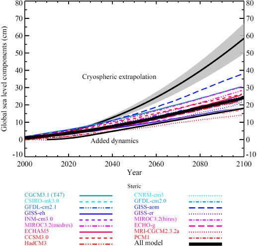
FIGURE 5.4 Committee projections of individual components of global sea-level rise. The colored lines are the steric contributions from various models with the A1B emission scenario, and the heavy black line (labeled “all model”) is the model average. Gray shading is the cryospheric contribution, and the black line within the gray swath is the cryosphere average. The black line at the bottom is the added ice dynamics component.
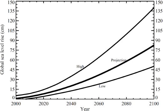
FIGURE 5.5 Range of committee projections for the sum of all individual components of global sea-level rise.
Table 5.2), interpolated between the years 2030, 2050, and 2100, and adding the lower fit (mean minus twice the standard deviation) of the extrapolated cryospheric estimate. For the high estimate, the steric curve plus twice the standard deviation of the steric values was added to the upper fit (mean plus twice the standard deviation) of the cryospheric extrapolation and the additional ice dynamics contribution.
All three curves in Figure 5.5 have a positive curvature, as do the semi-empirical projections. In the committee’s projection, the acceleration originates primarily from the cryospheric extrapolation, although a small amount of acceleration comes from the steric term. In the semi-empirical estimates, the acceleration is built into the mathematical expression relating the rate of sea-level rise to the departure of temperature from some equilibrium value (see the first two equations in “Semi-Empirical Models” above). In this formulation, as long as temperature continues to rise, sea-level rise will accelerate.
Given the inherent thermodynamics of ice bodies in disequilibrium with their climatic environment, an accelerating cryospheric contribution is a reasonable supposition as long as the timescales of the climatic change are short relative to the timescales of the ice response. Although large glaciers may have response timescales of a few decades, the Greenland and Antarctic ice sheets, which dominate the cryospheric term, have response times of centuries to millennia.
Figure 5.6 compares the ranges of sea-level rise projected by the committee, IPCC (2007), and Vermeer and Rahmstorf (2009). The committee’s projections for 2030 and 2050 are similar to the Vermeer and Rahmstorf (2009) projections, but have a wider range: 8–23 cm for 2030 and 18–48 cm for 2050. For 2100, when IPCC (2007) estimates are also available, the committee’s projected range (50–140 cm) is substantially higher than the IPCC (2007) range (18–59 cm, with an additional 17 cm if rapid dynamical changes in ice flow are included) and lower than the Vermeer and
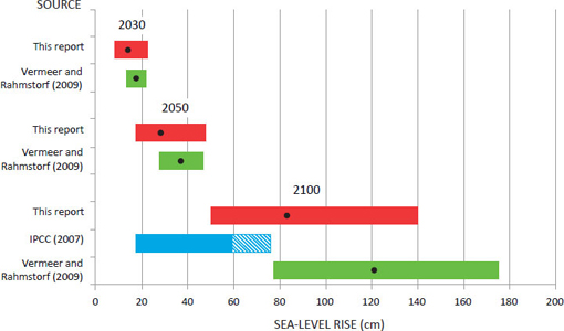
FIGURE 5.6 Global sea-level rise for 2030, 2050, and 2100 projected by this committee (red), Vermeer and Rahmstorf (2009; green), and IPCC (2007; blue). The dots are the projected values and the colored bars are the ranges. The IPCC value includes the sea-level projection (blue) plus the scaled-up ice sheet discharge component (blue diagonal lines).
Rahmstorf (2009) range (78–175 cm). The committee’s results differ from the IPCC (2007) results because the committee considered more recent scientific observations and modeling and also used different methods to make projections. For example, although the steric contributions were drawn from the same global climate models used in IPCC (2007), the committee used the global climate model results directly, whereas IPCC (2007) used lower-order models to develop estimates for emission scenarios that were not simulated in global climate models (e.g., A1FI). In addition, the committee used extrapolation methods to project the cryosphere component of sea-level rise, whereas IPCC (2007) used climate models.
The global sea-level projections shown in Figures 5.4 and 5.5 do not include contributions from groundwater depletion and reservoir extraction. Estimates available at the time this report was being written (e.g., Milly et al., 2010) suggested that the sum of these contributions was near zero, within the stated uncertainties. Although some studies have pointed out that the number of new reservoirs has been declining over the past three decades (e.g., Chao et al., 2008), the committee had no firm basis for projecting a growing contribution to sea-level rise from groundwater extraction. A new paper published as this report was nearing release, however, projects that increasing groundwater extraction and decreasing reservoir impoundment will contribute about 1.5 ± 0.8 cm SLE to global sea level in 2030, 3.1 ± 1.1 cm SLE in 2050, and 7.5 ± 2.0 cm SLE in 2100 (Wada et al., 2012b). If confirmed by subsequent analyses, these results indicate that changes in the balance of groundwater depletion and reservoir impoundment could increase the magnitude of future sea-level change.
PREVIOUS PROJECTIONS OF U.S. WEST COAST SEA-LEVEL RISE
Only a few studies have attempted to project 21st century sea-level rise along the west coast of the United States. Methods varied, but each study used global climate models forced by the IPCC (2000) low and high greenhouse gas emission scenarios. The results were then downscaled, used in semi-empirical projections, or combined with local information, as discussed below. Each of the studies emphasized that the results represented a range of outcomes, not formal projections of sea-level rise.
The earliest of these studies, Hayhoe et al. (2004), used two global climate models, downscaled to a 150 km2 grid, to simulate climate change in California. Projections of various aspects of climate change were averaged over the 2020–2049 and 2070–2099 periods, relative to the 1961–1990 period, following the approach taken in the IPCC Third Assessment Report. Hayhoe et al. (2004) estimated that sea level along the California coast would rise 8.7 cm to 12.7 cm for the 2020–2049 period, and 19.2 cm to 40.9 cm for the 2070–2099 period, depending on the model and emission scenario used.
Mote et al. (2008) estimated future sea-level rise off Washington for 2050 and 2100, dividing the coastline into three regions according to their vertical land motions. They used global climate models to calculate the thermal expansion and cryosphere contributions to sea-level rise. The rates of global sea-level rise were then adjusted for vertical land motions and for model-predicted seasonal and interannual wind-driven increases in sea level. Mote et al. (2008) projected low, medium, and high sea-level rise for the Puget Sound region of 16 cm, 34 cm, and 128 cm, respectively, by 2100. They also found that some parts of the Olympic Peninsula could experience tectonic uplift that would exceed the low end of projected rates of global sea-level rise, with the medium estimate for sea-level fall between 0 cm and -15 cm by 2050, depending on location, and 0 cm and -30 cm by 2100.
Cayan et al. (2009) projected sea-level rise off California using Rahmstorf’s (2007) semi-empirical method with global average surface air temperature simulated from global models. Assuming that the rate of sea-level rise off the California coast will be the same as the global rate, Cayan et al. (2009) estimated sea-level rise of 30–45 cm by 2050, and 50–140 cm by 2100, relative to 2000.
Tebaldi et al. (2012) projected sea-level rise at 11 tide gage locations along California, Oregon, and Washington using the semi-empirical method of Vermeer and Rahmstorf (2009) to estimate global sea-level rise and 50 years (1959–2008) of tide gage records to estimate local rates and their deviations from global sea-level rise caused by local effects. Based on this information and output from an ensemble of GCM
simulations, they obtained sea-level rise estimates of 3–12 cm by 2030 and 11–30 cm by 2050, relative to 2008, for the 11 locations.
COMMITTEE PROJECTIONS OF SEA-LEVEL RISE ALONG THE CALIFORNIA, OREGON, AND WASHINGTON COASTS
Sea-level rise along the west coast of the United States differs from global mean sea-level rise because of local steric (primarily thermosteric) contributions, dynamic height differences caused primarily by changes in winds, the gravitational and deformational effects of modern land ice melting, and vertical land motions along the coast (see Chapter 4). The committee projected the contributions of these components to sea-level rise off the California, Oregon, and Washington coasts for the years 2030, 2050, and 2100, relative to year 2000. The local steric and wind-driven contribution was estimated using GCMs; the land ice contribution, adjusted for gravitational and deformational effects, was extrapolated; and the contribution from vertical land motion was estimated using Global Positioning System (GPS) data. Values for the individual contributions are summarized in Table 5.3 and discussed below.
Steric and Dynamic Ocean Height Effects
The local steric and wind-driven components were determined from the same CMIP 3 global ocean models used to calculate the steric contribution to global sea-level rise. Thirteen of the CMIP 3 models examined in Pardaens et al. (2010) include global annual averages of the steric contribution and wind-driven dynamic ocean heights on a 1° latitude by 1° longitude grid. From this data set, the committee selected the ocean model grid points closest to the coastlines of California, Oregon, and Washington at each latitude, developing a time series for each model at each latitude. To obtain values
TABLE 5.3 Regional Sea-Level Rise Projections (in cm) Relative to Year 2000
| 2030 | 2050 | 2100 | ||||
| Component | Projection | Range | Projection | Range | Projection | Range |
| Steric and dynamic oceana | 3.6 ± 2.5 | 0.0–9.3 (B1-A1FI) | 7.8 ± 3.7 | 2.2–16.1 (B1-A1H) | 20.9 ± 7.7 | 9.9–37.1 (B1-A1F1) |
| Non-Alaska glaciers and ice capsb | 2.4 ± 10.2 | 4.4 ± 0.3 | 11.4 ± 1.0 | |||
| Alaska, Greenland, and Antarctica with sea-level fingerprint effectc | ||||||
| Seattle, WA | 7.1 | 5.4–9.5 | 16.0 | 11.1-22.1 | 52.7 | 32.7–74.9 |
| Newport, OR | 7.4 | 5.6–9.5 | 16.6 | 11.7–22.2 | 54.5 | 34.1–75.3 |
| San Francisco, CA | 7.8 | 6.1–9.6 | 17.6 | 12.7–22.3 | 57.6 | 37.3–76.1 |
| Los Angeles, CA | 8.0 | 6.3–9.6 | 17.9 | 13.0–22.3 | 58.5 | 38.6–76.4 |
| Vertical land motiond | ||||||
| North of Cape Mendocino | -3.0 | -7.5–1.5 | -5.0 | -12.5–2.5 | -10.0 | -25.0–5.0 |
| South of Cape Mendocino | 4.5 | 0.6–8.4 | 7.5 | 1.0–14.0 | 15.0 | 2.0–28.0 |
| Sum of all contributions | ||||||
| Seattle | 6.6 ± 5.6 | -3.7–22.5 | 16.6 ± 10.5 | -2.5–47.8 | 61.8 ± 29.3 | 10.0–143.0 |
| Newport | 6.8 t 5.6 | -3.5–22.7 | 17.2 ± 10.3 | -2.1–48.1 | 63.3 ± 28.3 | 11.7–142.4 |
| San Francisco | 14.4 ± 5.0 | 4.3–29.7 | 28.0 ± 9 2 | 12.3–60.8 | 91.9 ± 25.5 | 42.4–166.4 |
| Los Angeles | 14.7 ± 5.0 | 4.6–30.0 | 28.4 ± 9.0 | 12.7–60.8 | 93.1 - 24.9 | 44.2–166.5 |
a Projection indicates the mean and ± standard deviation computed for the Pacific coast from the gridded data presented in Pardaens et al. (2010) for the A1B scenario. Ranges are the means for B1 and A1Fl using the scaling in Table 10.7 of IPCC (2007; see also Table 5.1 of this report): (B1/A1B) = (0.1/0.13); (A1Fl/A1B) = (0.17/0.13).
b Extrapolated based on ice loss rates for glaciers and ice caps except Alaska, Greenland, and Antarctica. No ranges are given because these sources are assumed to have a small or uniform effect on the gradient in sea-level change along the U.S. west coast (see “Sea-Level Fingerprints of Modern Land Ice Change” in Chapter 4).
c Extrapolation based on ice loss rates and gravitational attraction effects for Alaska, Greenland, and Antarctica. Ranges reflect uncertainty in ice loss rates.
d Assumes constant rates of vertical land motion of 1.0 ± 1.5 mm yr-1 for Cascadia and -1.5 ± 1.3 mm yr-1 for the San Andreas region. The signs were reversed to calculate relative sea level. Uncertainties are 1 standard deviation.
for 2030, 2050, and 2100 (relative to year 2000) that reflect the century-long change in sea level rather than year-to-year variations, quadratic fits to each time series were performed. In addition, the variance about the quadratic curve was computed for 21-year intervals centered on 2030, 2050, and for the last 20 years of the time series. Figure 5.7 shows the sum of the steric and dynamic ocean height terms for the 13 models. Although some models predict a north-south gradient in sea-level change, the average for all of the models predicts nearly uniform steric and dynamic ocean height contributions along the entire coast (see heavy black line in Figure 5.7). The average values were used in the projection (see first row of Table 5.3).
Cryosphere and Sea-Level Fingerprint Effects
The contribution of the cryosphere to sea-level rise along the west coast of the United States is influenced by gravitational and deformational effects associated with melting from the Alaska glaciers, which are nearby, and the Greenland and Antarctic ice sheets, which are large (see “Sea-Level Fingerprints of Modern Land Ice Change” in Chapter 4). To account for these effects in the projections, the committee subdivided ice loss rates into four categories: Greenland Ice Sheet, Antarctic Ice Sheet, Alaska glaciers, and all other glaciers and ice caps. The sea-level fingerprint scale factors were applied to the first three sources, then loss rates from all ice sources were extrapolated forward and converted to cumulative sea-level rise (see details in Appendix E). Because the gravitational and deformational effects associated with the sea-level fingerprints of the three ice sources varies strongly with latitude, the projections were made for four points along the coast: Seattle, Washington, Newport, Oregon, San Francisco, California, and Los Angeles, California (Table 5.3). A polynomial was then fit through the four points to estimate the influence of the sea-level fingerprints as a function of latitude.
To determine the magnitude of the gravitational and deformational effects of melting in Alaska, Greenland, and Antarctica on the projections, the committee compared the results of the above analysis with the global cryosphere extrapolations, which were done without an adjustment for the regional sea-level fingerprints. The difference between the adjusted and
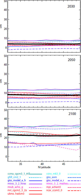
FIGURE 5.7 Combined thermosteric and ocean dynamic height sea-level change for 2030 (top), 2050 (middle), and 2100 (bottom), relative to 2000, from 13 GCMs as a function of latitude. The thick black line indicates the average of all the models.
unadjusted extrapolations is given in Table 5.4. The gravitational and deformational effects reduce the cryospheric contribution to relative sea-level rise projected for 2100 by 7–21 percent along the north coast and by 1–12 percent along the central coast. Along the south coast, these effects can increase the cryospheric contribution to sea-level rise by up to 2 percent or decrease it by up to 6 percent.
The projection assumes that the fingerprint scale factors remain constant for the small reduction in land ice volume expected by 2100, which is likely reasonable for the next several decades. Assuming that the sea-level fingerprint is correct, uncertainties in the calculation are associated with the ice loss rate. When uncertainties in the ice loss rate are factored in, the fingerprint-adjusted contribution of Alaska, Greenland, and Antarctica to relative sea-level rise ranges from 33–75 cm along the north coast and 39–76 cm along the south coast for 2100 (Table 5.3).
Vertical Land Motion
Major causes of vertical land motion along the west coast of the United States include tectonics, glacial isostatic adjustment (GIA), and subsidence as a result of sediment compaction and/or fluid withdrawal (see “Vertical Land Motion” in Chapter 4). The vertical land motion signal in Oregon, Washington, and northern California is dominated by regional tectonics associated with the Cascadia Subduction Zone. In California south of Cape Mendocino, vertical land motion depends on varying combinations of GIA, sediment compaction, fluid withdrawal or recharge, and local compressional tectonics that may or may not be related to the San Andreas Fault. Projections of the regional tectonic and GIA components of vertical land motion can be made using earthquake cycle deformation models and geophysical models, respectively. The total vertical land motion, including tectonics, GIA, compaction, and fluid withdrawal and recharge, can be projected using continuous GPS (CGPS), assuming that the vertical land motion is predominantly secular within ~100 years. Results from these three projection methods are summarized in Table 5.5 and discussed below.
Tectonic Projections
Tectonics causes significant vertical land motion along the coast above the Cascadia Subduction Zone. The tectonic component of vertical land motion in this area can be projected using earthquake cycle deformation models. The CAS3D-2 model (He et al., 2003; Wang et al., 2003; Wang, 2007), which is the most sophisticated and complete model of earthquake deformation along the Cascadia Subduction Zone, is the only model that has been used to make forward projections. Like other tectonic models, it is limited by incomplete knowledge of the temporal behavior of the earthquake process, such as the degree of periodicity of the Cascadia earthquake cycle, which adds uncertainties that are difficult to quantify. The model excludes vertical land motion from glacial isostatic adjustment.
The projected rates of interseismic deformation for the Cascadia Subduction Zone from the CAS3D-2 model are given in Table 5.5. The projections suggest that coastal sites, which are closest to the offshore subduction boundary, will undergo uplift, whereas more inland locations (Anacortes and Seattle) will undergo subsidence. Projected vertical land motions for the coastal sites range from -1.0 mm yr-1 (subsidence) to +3 mm yr-1 (uplift), with most rates varying by less than 0.2 mm yr-1 over the 21st century. The vertical land motions projected using the CAS3D-2 model
TABLE 5.4 Effect of Sea-Level Fingerprints of Alaska, Greenland, and Antarctica Ice Masses Expressed as Percentage Differences from Cryosphere Projections with No Fingerprint Effecta
| North Coast (Neah Bay) | Central Coast (Eureka) | South Coast (Santa Barbara) | |||||||
| Year | Low | Central | High | Low | Central | High | Low | Central | High |
| 2030 | -19.9% | -13.4% | -9.6% | -10.4% | -5.8% | -3.1% | -4.9% | -1.6% | 0.4% |
| 2050 | -20.3% | -12.2% | -8.6% | -10.6% | -4.8% | -2.2% | -5.1% | -0.8% | 1.2% |
| 2100 | -21.1% | -10.8% | -7.4% | -12.3% | -3.7% | -1.2% | -5.5% | 0.2% | 2.1% |
a Uncertainties, expressed as low-high values, were derived from the spread of projected contributions from Alaska, Greenland, and Antarctica.
TABLE 5.5 Vertical Land Motion Projections for the Two Tectonic Regimes
| Tectonic Component (mm yr-1)a | GIA Component(mm yr-1)b | Total Vertical Land Motion(mm yr-1)c | |||||
| Location | Latitude | Longitude | 2010–2030 | 2030–2050 | 2050–2100 | 2010–2100 | 2010–2100 |
| Cascadia Subduction Zone | |||||||
| Cherry Point, WA | 48.87 | -122.75 | 0.2 ± 0.4 | 1.0 ± 15 | |||
| Anacortes, WA | 48.56 | -122.64 | -0.9 | -0.9 | -1.0 | -0.1 ± 0.5 | 1.0 ± 15 |
| Seattle, WA | 47.85 | -122.73 | -0.6 | -0.6 | -0.6 | -0.5 ± 0.4 | 1.0 ± 15 |
| Long Beach, WA | 46.58 | -123.83 | 1.9 | 1.8 | 1.7 | -1.1 ± 0.5 | 1.0 ± 15 |
| Pacific City, OR | 45.38 | -123.94 | 1.7 | 1.6 | 1.5 | -1.0 ± 0.4 | 1.0 ± 1.5 |
| Waldport, OR | 44.42 | -124.02 | 1.7 | 1.6 | 1.5 | -0.9 ± 0.3 | 1.0 ± 1.5 |
| Coos Bay, OR | 43.36 | -124.30 | 2.3 | 2.2 | 2.1 | -0.9 ± 0.3 | 1.0 ± 1.5 |
| Eureka, CA | 40.87 | -124.15 | 3.0 | 2.8 | 2.6 | -0.7 ± 0.3 | 1.0 ± 1.5 |
| San Andreas Fault Zone | |||||||
| Point Reyes, CA | 38.00 | -122.98 | -0.5 ± 0.3 | -1.5 ± 1.3 | |||
| San Francisco, CA | 37.80 | -122.47 | -0.5 ± 0.3 | -1.5 ± 1.3 | |||
| Monterey, CA | 36.60 | -121.88 | -0.5 ± 0.3 | -1.5 ± 1.3 | |||
| Port San Luis, CA | 35.17 | -120.75 | -0.5 ± 0.3 | -1.5 ± 1.3 | |||
| Santa Monica, CA | 34.02 | -118.50 | -0.3 ± 0.3 | -1.5 ± 1.3 | |||
| Los Angeles, CA | 33.72 | -118.27 | -0.4 ± 0.3 | -1.5 ± 1.3 | |||
| San Diego, CA | 32.72 | -117.17 | -0.4 ± 0.3 | -1.5 ± 1.3 | |||
NOTE: Positive rates denote uplift and negative rates denote subsidence.
a Rates provided by Kelin Wang, Geological Survey of Canada, using the CAS3D-2 model described in Chapter 4.
b Rates were averaged from an ensemble of 16 GIA models (see Table 4.3) and are represented so positive GIA means falling relative sea level.
c Rates (± 1 standard deviation) were determined from CGPS data from the Scripps Orbit and Permanent Array Center taken within 15 km of the coast; see Table A.1.
generally agree with rates determined from leveling (Burgette et al., 2009) and from GPS (Mazzotti et al., 2008; this report).
GIA Projections
Projections of the GIA component of vertical land motion were made using an ensemble of 16 models. The projections show subsidence at all locations except for northernmost Washington, which shows negligible uplift (Table 5.5). Mean GIA model predicted rates of vertical land motion range from +0.2 mm yr-1 in northernmost Washington to -1.0 mm yr-1 in southern Washington and northern Oregon. This strong latitudinal gradient illustrates the importance of GIA in regions underneath or at the margins of the extinct Laurentide ice sheet. In southern Oregon and California, mean rates are generally between -0.4 mm yr-1 and -1.0 mm yr-1. Given the slow pace of glacial isostatic adjustment, these rates are assumed constant for the three projection periods (2030, 2050, and 2100).
GPS Projections
The total vertical land motion, including signals from tectonics, GIA, sediment compaction, and/or fluid withdrawal or recharge, is recorded in GPS data. Consequently, the committee used CGPS data in its projections of sea-level rise for 2030, 2050, and 2100. It would be attractive to use the relatively densely-spaced CGPS vertical land motion data to make projections at high spatial resolution along the coast. However, vertical land motions can vary at length scales that are considerably smaller than the CGPS station spacing, so interpolation using the CGPS data carries substantial risk of spatial aliasing. Moreover, the data exhibit significant scatter because of local sediment compaction and/or fluid withdrawal (see Figure 4.14b and associated discussion). Consequently, the committee chose the conservative approach of projecting vertical land motion for the two tectonic regions—Cascadia and the San Andreas region—and characterizing them using simple statistics (mean and 1 standard deviation). With obvious outliers removed, the current rates of vertical
land motion for these regions are 1.0 ± 1.5 mm yr-1 for Cascadia and -1.5 ± 1.3 mm yr-1 for the San Andreas area.
In using the current rates of vertical land motion in its projections, the committee assumed that the CGPS spatial pattern and rates in the two tectonic regions would remain constant for 2030, 2050, and 2100. This assumption is supported by leveling data in California (Appendix D) and in Washington and Oregon (Burgette et al., 2009). In addition, the CAS3D-2 tectonic model suggests that, in the absence of a great earthquake, the general vertical land motion pattern or trend in Cascadia will not change significantly in the coming century. The projected rates of vertical land motion are given in Table 5.3.
Discussion of Regional Projections
The projections of sea-level rise off California, Oregon, and Washington were made by summing the cryosphere component, adjusted for the effects of the sea-level fingerprints of Alaska, Greenland, and Antarctica; the local steric and dynamical ocean component; and the vertical land motion component. The values used for the projections appear in Table 5.3 and are illustrated in Figure 5.8. The cryosphere is the only component with pronounced upward curvature (acceleration) over the 21st century. Ice mass loss rates for Alaska, Greenland, and Antarctica were adjusted for gravitational and deformational effects and then added to loss rates from other glaciers and ice caps. The sum was then extrapolated forward. The steric and dynamical ocean components (blue swath in Figure 5.8) were extracted from the ocean data provided by Pardaens et al. (2010), averaged for the west coast, then smoothed for plotting using locally weighted regression. The vertical land motion components and their uncertainties for the northern and southern part of the coast are shown in the shaded areas; the bars on the right margin indicate the range for 2100. North of Cape Mendocino, the coast is experiencing mean uplift, so vertical land motion contributes negatively to relative sea-level rise (although uncertainties are large and include positive contributions), whereas the coast south
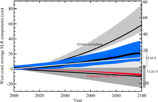
FIGURE 5.8 Committee projections of components of sea-level rise off California, Oregon, and Washington. The blue band represents the model results for combined global steric and local dynamical sea-level change, averaged between 32° and 49° latitude, from 13 GCMs. Light gray shading in the middle of the figure shows estimated effects of vertical land movement in the San Andreas region (VLM S), and dark gray shading at the bottom of the figure shows the vertical land movements for Cascadia (VLM N). Light gray shading at the top of the figure shows the global cryosphere, including added ice dynamics. The red line is the effect of the sea-level fingerprint of ice melt from the Alaska, Greenland, and Antarctica sources, shown for the north coast (49°N). The fingerprint effect is subtracted from the global cryosphere.
of Cape Mendocino is experiencing mean subsidence, so vertical land motion contributes positively to relative sea-level rise.
Figure 5.9 shows the total regional sea level projected for the years 2030, 2050, and 2100, relative to year 2000, for a transect along the west coast. The shape of the curve is dominated by the change in vertical land motion at about 40° latitude from uplift in the north to subsidence in the south. The sea-level fingerprint effect reduces the projected sea levels along the entire coast and is most pronounced in Washington. The fingerprint effect has not been included in previous studies and projections of sea level for the west coast (e.g., Mote et al., 2008; Cayan et al., 2009; Tebaldi et al., 2012). The ocean components have little effect on the north-south gradient in projected sea-level change.
The committee’s projections for the west coast of the United States are significantly different from global projections (Figure 5.10). The difference is largest off the Washington coast, where sea-level fingerprint effects lower the height of the ocean surface and regional tectonics raises the height of the land surface, resulting in rates of relative sea-level rise that are substantially lower than the global mean. Off the California coast, where subsidence is lowering the land surface, the projected relative sea-level rise is slightly higher than the global mean. The committee’s projected values for California are somewhat lower than the Vermeer and Rahmstorf (2009) projections, which are being used by California state agencies on an interim basis for coastal planning (CO-CAT, 2010). For California and Washington, the committee’s projections fall within the range presented in Cayan et al. (2009) and Mote et al. (2008), respectively. The committee’s projected values for 2030 and 2050 also are comparable to those of Tebaldi et al., (2012), although the committee found a larger north-south difference in the magnitude of sea-level rise.
Projections of future sea-level rise carry numerous sources of uncertainty. This uncertainty arises from an incomplete understanding of the global climate system, the inability of global climate models to accurately represent all important components of the climate system at global or regional scales, a shortage of data at the temporal and spatial scales necessary to constrain the models, and the need to make assumptions about future conditions (e.g., population growth, technological developments, large volcanic eruptions) that drive the climate system. Although a systematic analysis of these uncertainties was beyond the ability of the committee, this report attempts to describe and combine the most important uncertainties. For the committee’s global sea-level rise projections, important uncertainties are associated with assumptions about the growth of concentrations of greenhouse gases and sulfate aerosol, which affect the steric contribution, and future ice loss rates and the effect of rapid dynamic response, which affect the land ice contribution. Additional, unquantified uncertainties arise from neglecting the terrestrial water component in the projections and from combining model-projected steric contributions with extrapolation-projected land ice contributions (e.g., model projections account for future emissions whereas extrapolations do not).
Regional projections carry additional uncertainties because more components are included and some components are estimated from global scale analyses. The uncertainties are larger for the committee’s projections for California, Oregon, and Washington than they are for the global projections, primarily because uncertainties in the steric component are larger at smaller spatial scales and because some of the additional components (e.g., vertical land motion) have relatively large uncertainties.
For both global and regional projections of sea-level rise, uncertainties grow as the projection period increases because the chances of the observations and models deviating from actual climate changes increases. Currently, all projection methods—including process-based numerical models, extrapolations, and semi-empirical methods—have large uncertainties at 2100. Although the actual value of sea-level rise will almost surely fall somewhere within these wide uncertainty bounds, confidence in specifying the exact value is relatively low. At short timescales, the models more closely represent the future climate system, so uncertainties are smaller and confidence is higher. Confidence in the committee’s projections is likely to be highest in 2030 and perhaps 2050, which are likely of greatest interest to coastal planners, engineers, and other decision makers tasked with planning for sea-level rise along the west coast of the United States.
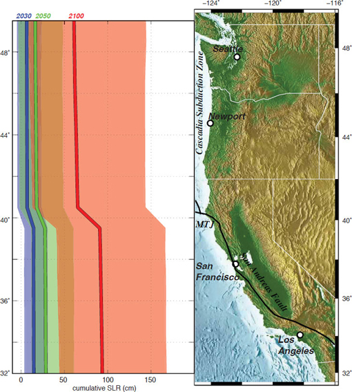
FIGURE 5.9 Projected sea-level rise off California, Oregon, and Washington for 2030 (blue), 2050 (green), and 2100 (pink), relative to 2000, as a function of latitude. Solid lines are the projections and shaded areas are the ranges. Ranges overlap, as indicated by the brown shading (low end of 2100 range and high end of 2050 range) and blue-green shading (low end of 2050 range and high end of 2030 range). MTJ = Mendocino Triple Junction, where the San Andreas Fault meets the Cascadia Subduction Zone.
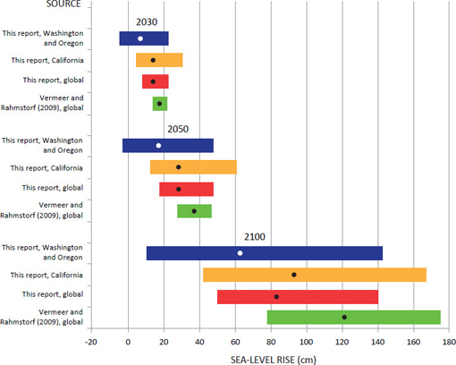
FIGURE 5.10 Committee’s projected sea-level rise for California, Oregon, and Washington compared with global projections. The dots are the projected values and the colored bars are the ranges. Washington and Oregon = coastal areas north of Cape Mendocino; California = coastal areas south of Cape Mendocino.
Extreme events can raise sea level much faster than projected above. The rapid rise in sea level could be temporary, as in the case of a severe storm, or permanent, as in the case of a great subduction zone earthquake. The potential contribution of such extreme events to future sea-level rise is described below.
Extreme Sea Level
In the first 3 months of 1983, the west coast of the United States experienced a sequence of strong storms, with the coincidence of El Niño conditions, high astronomical tides, and large waves producing record sea levels along virtually the entire coast (see “Changes in Ocean Circulation” in Chapter 4). Damage was extensive (e.g., Figure 5.11), with losses totaling $215 million (in 2010 dollars; Griggs et al., 2005). Some models predict that such extreme events will become more common and that heightened sea level will persist longer as sea level rises, increasing the potential for damage (Cayan et al., 2008; Cloern et al., 2011).
Cloern et al. (2011) used a GCM forced by the IPCC (2000) B1 emission scenario to assess possible climate change impacts in the San Francisco Bay and delta. As part of the analysis, they used a local sea-level model, introduced by Cayan et al. (2008), to investi-
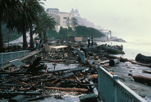
FIGURE 5.11 Rio Del Mar on northern Monterey Bay was damaged during the El Niño winter of 1983 by large waves arriving simultaneously with high tides and elevated sea levels. SOURCE: Courtesy of Gary Griggs, University of California, Santa Cruz.
gate sea-level extremes that occur in conjunction with broad-scale sea-level rise. Historical (1961–1999) and projected (2000–2100) hourly sea level was simulated using predicted tides, simulated weather and El Niño-Southern Oscillation conditions, and long-term rates of sea-level rise from Vermeer and Rahmstorf (2009). Wind, surface atmospheric pressure, and tropical Pacific sea surface temperature were obtained from the National Center for Atmospheric Research PCM1 climate model simulation.
The committee reproduced the Cloern et al. (2011) analysis using its own sea-level projection for the San Francisco area and the Geophysical Fluid Dynamics Laboratory CM2.1 model. This exercise showed that as mean sea level rises, the incidence of extreme high-sea-level events becomes increasingly common (Figure 5.12). According to the model, the incidence of extreme water heights that exceed the 99.99th percentile level (1.41 m above historical mean sea level) increases from the historical rate of approximately 9 hours per decade to more than 250 hours per decade by mid-century, and to more than 12,000 hours per decade by the end of the century. The model also shows that the duration of these extremes would lengthen from a maximum of 1 or 2 hours for the recent historical period to 6 or more hours by 2100, increasing the exposure of the coast to waves.
The marked rise in the occurrence of extreme sea levels is qualitatively similar for different sea-level rise scenarios, but the duration of extremes can differ substantially. For example, for the low end of the Vermeer and Rahmstorf (2009) sea-level projection (78 cm by 2100), extreme water heights (exceeding the 99.99th percentile) are predicted to occur more than 300 hours per decade by 2050 and more than 7,500 hours per decade by 2100.
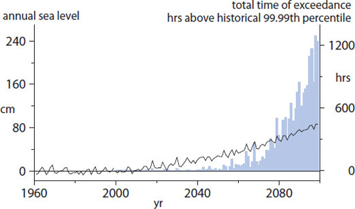
FIGURE 5.12 Projected number of hours (blue bars) of extremely high sea level off San Francisco under an assumed sea-level rise and climate change scenario. In this exercise, a sea-level event registers as an exceedance when San Francisco’s projected sea level exceeds its recent (1970–2000) 99.99th percentile level, 1.4 m above historical mean sea level. In the recent historical period, sea level has exceeded this threshold about one time (1 hour) every 14 months. Sea-level rise (black line) during 1960–1999 was arbitrarily set to zero, then increased to the committee’s projected level for the San Francisco area over the 21st century (92 cm). SOURCE: Adapted from Cloern et al. (2011).
Great Earthquakes Along the Cascadia Subduction Zone
Measurements of current deformation and geologic records (e.g., Savage et al., 1981; Atwater, 1987; Nelson et al., 1996; Atwater and Hemphill-Haley, 1997) establish the potential for great (magnitude greater than 8) megathrust earthquakes and catastrophic tsunamis along the Cascadia Subduction Zone. In Washington and Oregon, a great earthquake would cause some areas to immediately subside and sea level to suddenly rise perhaps by more than 1 m. This earthquake-induced rise in sea level would be in addition to the relative sea-level rise projected above. A great earthquake also would produce large postseismic vertical land motions in the area for years to decades.
Sudden subsidence during great earthquakes is revealed in the geological record as abrupt changes in sedimentary sequences (Nelson, 2007). When a great earthquake occurs, salt marsh or terrestrial soils are lowered into the intertidal zone, killing the vegetation (e.g., Figure 5.13). These peaty soils are quickly covered by tsunami-deposited sand or muddy tidal sediments. In the decades after an earthquake, the coast slowly rises, producing a gradual transition back to a salt marsh or terrestrial soil (e.g., Nelson et al., 1996; Leonard et al., 2010).
Cycles of buried peat-mud couplets beneath coastal marshes (Figure 5.14) suggest that 6 to 12 great earthquakes have occurred at irregular intervals ranging from a few hundred years to 1,000 years along the central Cascadia margin over the past 6,000 years (Long and Shennan, 1998). Geologic evidence also has been found for six great earthquakes along the northern Oregon coast in the past 3,000 years (Darienzo and Peterson, 1995), 11 or 12 great earthquakes in southern Oregon in the past 7,000 years (Kelsey et al., 2002; Witter et al., 2003), and seven great earthquakes in southwest Washington in the past 3,500 years (Atwater and Hemphill-Haley, 1997). Turbidite deposits identified in marine cores suggest that 18 great earthquakes ruptured at least the northern two-thirds of the Cascadia margin during the Holocene (Goldfinger et al., 2003, 2008).
The last great earthquake on the Cascadia megathrust occurred on January 26, 1700 (Satake et al., 1996, 2003). The date of the earthquake was determined by radiocarbon dating of suddenly buried marsh herbs, tree-ring records of trees stressed by coastal flooding
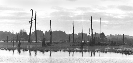
FIGURE 5.13 Ghost forests, such as this grove of weather-beaten cedar trunks near Copalis River, Washington, are evidence of sudden subsidence. SOURCE: Courtesy of Brian Atwater, U.S. Geological Survey.
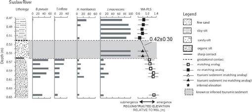
FIGURE 5.14 Stratigraphy and abundance of foraminifera in the sediment sequence recording the 1700 earthquake at Siuslaw River, Oregon. Also shown is a reconstruction of elevation during this interval (WA-PLS column). Sediment likely deposited by tsunamis is shaded in gray. SOURCE: Modified from Hawkes et al. (2011).
during subsidence (e.g., Yamaguchi et al., 1997), and Japanese historical records of a tsunami from a distant source. Modeling of the tsunami waveform (Satake et al., 1996) and estimates of coastal subsidence based on detailed microfossil studies (Hawkes et al., 2011) suggest an earthquake magnitude of 8.8 to 9.2. The coastal subsidence and associated sea-level rise were spatially variable, with the largest rise in sea level (1–2 m) occurring in northern Oregon and southern Washington, where the plate boundary forms a wide, shallow arch (Leonard et al., 2004, 2010; Hawkes et al., 2011). Other sections of the margin subsided <1 m and the southernmost part of the subduction zone was uplifted (Leonard et al., 2004, 2010; Hawkes et al., 2011).
Discussion
Changes in regional meteorological and climate patterns, including El Niños, coupled with rising sea level, are predicted to result in increasing extremes in sea levels. Models suggest that sea-level extremes will become more common by the end of the 21st century. Waves riding on these higher water levels will cause increased coastal damage and erosion—more than that expected by sea-level rise alone.
The biggest game changer for future sea level along the west coast of the United States is a great Cascadia earthquake. The related coastal subsidence of such an earthquake would, in a matter of minutes, produce significantly higher sea levels off the Cascadia coast than 100 years of climate-driven sea-level rise. A great earthquake could cause 1–2 m of sea-level rise in some areas, which is significantly higher than the committee’s projection for Cascadia in 2100 (0.6 m). Further, the earthquake-induced sea-level rise would be an addition to the expected global warming-related sea-level rise.
Global projections are commonly made using ocean-atmosphere GCMs, which provide a reasonable representation of the steric contribution to global sea-level rise, but do not yet fully capture the cryospheric contribution. The IPCC (2007) projections made using this method are likely too low, even with an added ice dynamic component. Some studies project the cryospheric contribution by extrapolating current observations into the future, but the results depend on assumptions about the future behavior of the system. Semi-empirical methods avoid these difficulties by projecting global sea-level rise based on the observed relationship between sea-level change and global temperature. However, the highest projections made using this method (e.g., Grinsted et al., 2009) require unrealistically rapid acceleration of glaciological processes.
Given the strengths and weaknesses of the different projection approaches and the resource constraints of an NRC study, the committee chose to use GCMs developed for the IPCC Fourth Assessment Report to estimate the steric contribution and extrapolation techniques to estimate the cryospheric contribution. The contributions were then summed. The land hydrology component was assumed to be near zero and was not factored into the projection. The committee’s global projections for 2100 are substantially higher than the IPCC’s (2007) projection, mainly because of a faster growing cryosphere component, and are somewhat lower than the Vermeer and Rahmstorf (2009) projections. The committee estimates that global sea level will rise 8–23 cm by 2030, 18–48 cm by 2050, and 50–140 cm by 2100, relative to 2000 levels. As the projection horizon lengthens, the uncertainties grow, and hence the ranges widen. The major sources of uncertainty in the global projection are related to assumptions about the increase in rapid ice dynamics and the growth of future greenhouse gas emissions.
Formal projections of future sea-level rise along the west coast of the United States have not been made, although a few studies have presented ranges of possible outcomes for California and Washington. Methods vary but usually involve a combination of global models and local information. The committee’s projections account for factors that affect sea level in the area, including local steric variations; wind-driven differences in ocean heights; the gravitational and deformational effects associated with melting of Alaska, Greenland, and Antarctic glaciers; and vertical land motions along the coast. The local steric and wind-driven components were estimated by extracting northeast Pacific data from the same ocean models used for the global projections. The cryosphere component was adjusted for gravitational and deformational effects and then extrapolated forward. Vertical land motion was estimated using continuous GPS measurements.
The projected values vary by latitude, with the highest sea levels expected off the coast south of Cape Mendocino (4–30 cm for 2030, 12–61 cm for 2050, and 42–167 cm for 2100, relative to 2000) and the lowest sea levels expected off the coast north of Cape Mendocino (-4–23 cm for 2030, -3–48 cm for 2050, and 10–143 cm for 2100). The lower sea levels projected for Washington, Oregon, and northernmost California reflect coastal uplift and gravitational and deformational effects, which lower the relative sea level. Major sources of uncertainties in the regional projections are related to assumptions about the rate of future ice losses and the constant rate of vertical land motion over the projection period. Uncertainties are larger for the regional projections than for the global projections because more components are considered and because uncertainties in the steric and ocean dynamic components are larger at a regional scale than at a global scale.
Extreme events can raise sea level much faster than the rates projected by the committee. For example, unusually high sea levels may occur temporarily when major storms coincide with high astronomical tides, and especially during years when regional sea levels are anomalously heightened during El Niño events. As mean sea level continues to rise, the number of extreme high water events and their duration are expected to increase. A simulation based on predicted tides, projected weather and El Niño conditions under a mid-range greenhouse gas emission scenario, and the committee’s projections of sea-level rise suggests that the incidence of extreme water heights in the San Francisco Bay area would increase from about 9 hours per decade for the recent historical period (1961–1999) to hundreds of hours per decade by 2050 and several thousand hours per decade by 2100. In addition, the duration of these extremes would lengthen from 1 or 2 hours in the historical period to about 6 hours by 2100.
The biggest game changer for future sea-level rise along the U.S. west coast would be a great earthquake (magnitude greater than 8) along the Cascadia Subduction Zone. Such earthquakes have occurred every several hundred to 1,000 years, with the most recent occurring in 1700. During a great earthquake, some land areas would immediately subside and relative sea level would suddenly rise, perhaps by 1 m or more. This earthquake-induced rise in sea level would be added to the projected rise in relative sea level (about 60 cm by 2100).


