
In its Phase I report, the committee made several specific recommendations to alter the ways in which the hospital wage index (HWI) and the physician geographic practice cost indexes (GPCIs) are computed. During the committee’s second year, simulations were run to obtain the estimated payment impact for each of the committee’s recommended changes, using the best available data. Methods used and detailed findings from the simulations are provided in Appendix A-1, and Appendix A-2 provides 10 annotated Excel files with the hospital and physician payment simulation data reviewed by the committee (see http://www.iom.edu/GeoAdjustPaymentSimulations). This chapter presents highlights from the simulations and uses them to assess the effects that the committee’s recommendations could have on health care shortage areas or at-risk populations and providers.
By definition, implementation of a geographic adjustment results in redistribution of payments but not a change in aggregate payment. The changes recommended in the Phase I report were made to improve the technical accuracy of the price adjusters as measures of market-level variation in health care input prices.
In areas where simulated payments under the proposed changes are higher than payments under current policy, the committee interprets this as evidence that current Centers for Medicare & Medicaid Services (CMS) prices have been underpaying providers by not accurately accounting for exogenous factor prices. Conversely, in areas where simulated payments are lower than payments under current policy, the committee interprets this as evidence that providers have been overcompensated for services delivered. Over- or underpayment may be due to correctable technical shortcomings in the current index construction. It may also reflect intentional cross-subsidization or other payment redistributions implemented by the Medicare program to achieve policy objectives that are unrelated to input price differences.1
______________
1 An example of an intentional cross-subsidization is the rural floor for hospitals, a policy that states that hospitals in metropolitan areas must have indexes that are at least as high as the rural indexes in that state. Because this provision is budget-neutral, other hospitals not in these metro areas that benefit from the rural floor must essentially “fund” their higher index by accepting payment decreases. Notably, the frontier floors are not an example of an intentional cross-subsidization because the provision is budget-neutral.
Seven of the committee’s 15 recommendations from Phase I directly affected HWI or GPCI computations. These are listed in Box 2-1.
Some recommendations could not be included in our simulations due to lack of data.2 For ease in following the material in this chapter, Table 2-1 lists the recommendations as proposed for the hospital index and for the physician price adjusters, or GPCIs. This table categorizes recommendations into three groups: those that reflect technical improvements to data sources and/or computation methods; those that affect the definitions of labor markets or payment areas; and those that reflect elimination of policy adjustments that are currently incorporated into the hospital and physician indexes.
It is important to keep in mind that the Phase I report did not take a position for or against the objectives underlying various policy adjustments. The committee has, however, made a clear statement that it does not believe that the HWI and GPCIs are effective vehicles for implementing policy-motivated payment redistribution. The recommendations in the Phase I report were intended to improve the technical accuracy of the indexes and ensure their integrity as measures of geographic variation in input prices. Under the committee’s recommendations, the resulting hospital and physician indexes do not reflect any special treatment for providers located in areas currently affected by policy adjustments.
All of the committee’s recommended changes to the indexes have been implemented in the simulation as “budget-neutral” to the estimated payments under current policy. This means that total payments estimated under the committee’s proposed indexes must be the same as total payments estimated under current policy. The impact analyses thus focus only on the redistribution effects—that is, variation across areas or providers in the size of the payment impact. The hospital index findings present changes across hospitals or across labor markets (payment areas), while the physician index findings present changes across counties or across payment areas.
The committee believes that each of these changes improves the accuracy of the HWI or GPCIs as technical measures of variation in local input prices. The combined payment effects as presented in this chapter thus represent the committee’s best estimate of the inaccuracy present in the current hospital and physician payment system, whether due to data shortcomings, market misclassification, or potentially mistargeted policy adjustments. By removing the policy adjustments from the index computations, the committee is not recommending the elimination of policy adjustments in the payment systems, only that policy adjustments should not be implemented through the geographic price adjusters.
______________
2 For example, recommendations related to the rent component of the PE-GPCI could not be included in the simulations because the Phase I report indicated the data were not accurate and a reasonable proxy was not available. The Institute of Medicine (IOM) committee recommended developing new data on geographic variation in commercial rents, and although we reviewed survey data from other existing sources, none of them had sufficient geographic detail on a price-per-square-foot basis to be used as a next-best alternative for the computations in this chapter. Simulations therefore use the same Department of Housing and Urban Development rent data as CMS uses now. Other recommendations were included in the simulations using best available substitute data. For example, the committee also recommended that CMS work with the Bureau of Labor Statistics to obtain better data on geographic variation in employee benefits for health care workers, because benefit data as currently collected by that agency does not have sufficient geographic detail. In this instance, we do have a measure of market-level variation in hospital worker benefits through information on Medicare cost reports. The committee determined that an independent benefits index constructed from this information would be a reasonable proxy and would be preferable to constructing the wage indexes from base hourly wage data alone.
BOX 2-1
Phase I Recommendations Pertaining to Payment Simulations
The committee’s Phase I report made 15 recommendations, of which 7 were directly related to the computation of the geographic price indexes and were able to be incorporated into the payment simulations.
• Recommendation 2-1: The same labor market definition should be used for both the hospital wage index (HWI) and physician geographic adjustment factor. Metropolitan statistical areas and statewide nonmetropolitan statistical areas should serve as the basis for defining those labor markets.
• Recommendation 2-2: The data used to construct the HWI and the physician geographic adjustment factor should come from all health care employers.
• Recommendation 3-3: The committee recommends use of all occupations as inputs in the HWI, each with a fixed national weight based on the hours of each occupation employed in hospitals nationwide.
• Recommendation 4-1: The committee recommends that wage indexes be adjusted by using formulas based on commuting patterns for health care workers who reside in a county located in one labor market but commute to work in a county located in another labor market.
• Recommendation 4-2: The committee’s recommendation (4-1) is intended to replace the system of geographic reclassification and exceptions currently in place.
• Recommendation 5-4: The practice expense (PE) geographic practice cost index should be constructed with the full range of occupations employed in physicians’ offices, each with a fixed national weight based on the hours of each occupation employed in physicians’ offices nationwide.
• Recommendation 5-7: Nonclinical labor-related expenses currently included under PE office expenses should be geographically adjusted as part of the wage component of the PE.
SOURCE: IOM, 2011.
The two panels in Figure 2-1 show that the payment impact of the committee’s recommendations is relatively small for the large majority of Inpatient Prospective Payment System (IPPS) hospital and physician services. With respect to the HWI, 88 percent of IPPS discharges are from hospitals where the overall payment impact is less than 5 percent in either direction, and for 61 percent of discharges from hospitals, the payment impact is between -1 and 5 percent.3 Hospitals where payment drops by 10 percent or more represent 2.3 percent of discharges, and hospitals where payment increases by 10 percent or more represent 0.3 percent of discharges. With respect to the physician GPCIs, 96 percent of Part B relative value units (RVUs) are billed in counties where the overall payment impact is less than 5 percent in either
______________
3 This represents 84 and 62 percent of hospitals respectively (for the −5 to 5 percent range and −1 to 5 percent range) and 88 and 25 percent of counties respectively (for the −5 to 5 percent range and −1 to 5 percent range) for the physician payments.
| Type of Recommendation | Institutional Payments: HWI | Physician Payments: GPCI | ||
| Changes in Data |
|
|
||
| Changes in Payment Areas (Market Definitions) |
|
|
||
| Policy Changes in Exceptions and Adjustments |
|
|
||
NOTE: BLS = Bureau of Labor Statistics; CBSA = core-based statistical area; GPCI = geographic practice cost index; HWI = hospital wage index.
SOURCE: IOM, 2011.
direction, and for 67 percent of RVUs billed the payment impact is between −1 and 5 percent. Counties where payments are reduced by 10 percent or more represent 0.1 percent of RVUs, and counties where payment increases by 10 percent or more represent 0.3 percent of RVUs.
Although the aggregate payment impact is zero by design, the positive and negative effects are not randomly distributed across payment areas. Lower physician payments are estimated for 82 percent of counties, for example, and these counties tend to be smaller and located in rural areas. Forty-one percent of hospitals are located in areas with lower estimated diagnosis-
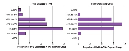
NOTE: GPCI = geographic practice cost index; HWI = hospital wage index; IPPS = Inpatient Prospective Payment System; RVU = relative value unit.
SOURCE: RTI simulations.
related group payments under the committee’s recommendations, but these reductions are not concentrated in specific types of hospitals nor are they more severe in rural versus urban areas.
The remainder of this chapter provides additional information on the impact of changes to the HWI as well as the impact of changes to the GPCIs. Boxes are provided in each of these sections with a review of how the geographic price adjuster is computed under current policy. The final section of this chapter summarizes what the committee has identified as the key findings from the payment simulations.
The distribution of estimated payment changes to hospitals paid under the inpatient prospective payment system is shown in Figure 2-2. The unit of observation in these graphs is the IPPS hospital. The upper frame identifies the impact of all recommended changes while the lower frame shows an estimate of the isolated impact of moving from the CMS hospital data source to the Bureau of Labor Statistics (BLS) data source. The two graphs together demonstrate that (1) hospitals in state nonmetropolitan markets tend to benefit under the BLS data change, but (2) the impact of other changes recommended by the committee offsets this effect in several areas. Under a comparison of simulated payments using the benefits-adjusted BLS-based index4 versus simulated payments using the CMS occupation-mix adjusted wage index, 78 percent of nonmetropolitan hospitals have higher payments under the BLS-based index.5 When all of the committee’s recommendations for the HWI are included in the simulations, that figure drops to 64 percent, owing primarily to the elimination of hospital labor market reclassification. In total, however, the simulations show that the committee’s recommendations have no effect on the aggregate rural—urban distribution of IPPS payments.
The move from hospital-reported data to BLS data affects individual market index values in both directions, but areas with the most extreme changes (those at either tail of the distribution in the lower frame of Figure 2-2) tend to be the smaller metropolitan markets where only one or two hospitals contribute to the CMS index. In larger markets where the CMS wage index value is derived from multiple hospitals, the relative wages computed from BLS data are more closely correlated with the occupation-mix adjusted relative wages from CMS data. To the extent that relative hospital wages are an unreliable proxy for relative wages in the health care industry as a whole, this suggests that the problem may lie in small or unstable samples of hospitals (in CMS’s hospital reported data) more than with inherent differences between hospitals and other parts of the industry.
The only change to market areas that was recommended for the HWI is the use of commuter data to “smooth” the differences between indexes at borders where health care workers commute across market areas. (For a recap of the commuter smoothing method the committee has recommended, see Box 2-2.) Smoothing adjustments for the HWI are generally small (25th to 75th percentile is −0.1 to +0.1 percent, with a minimum value of −1.8 percent and a few counties with increases as high as 6 to 8 percent). They behave as expected: commuting is more common from lower to higher wage areas, such that adjustments are more often positive than negative, and adjustments are largest for rural counties located adjacent to metropolitan areas.
______________
4 The term BLS-based index refers to the construction of the HWI and the GPCIs using BLS Occupational Employment Statistics wage data.
5 Each wage index was first adjusted for budget neutrality such that total simulated payments remain equal to total estimated payments under current CMS policy.
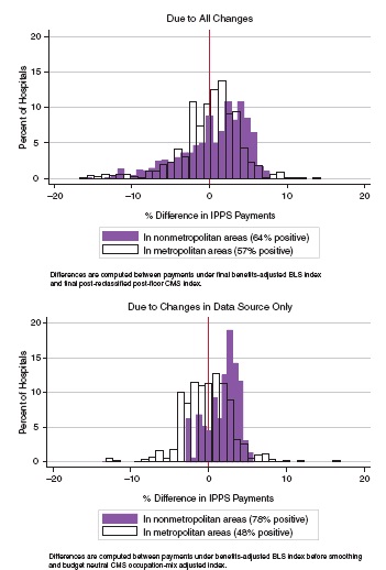
FIGURE 2-2 Distribution of payment effects of IOM committee recommendations on the hospital index.
NOTE: BLS = Bureau of Labor Statistics; CMS = Centers for Medicare & Medicaid Services; IPPS = Inpatient Prospective Payment System.
SOURCE: RTI simulations.
BOX 2-2
Summary of the Committee’s Commuter Smoothing Recommendation
The committee’s recommendation: The committee recommends that wage indexes be adjusted using formulas based on commuting patterns for health care workers who reside in a county located in one labor market but commute to work in a county located in another labor market.
Justification for recommendation: The committee recommends commuting pattern-based smoothing because it is anchored in a solid conceptual framework linking commuting with economic integration and therefore with labor markets. It is also consistent with the way metropolitan statistical areas (MSAs) are defined. Commuting patterns of health care workers are an indication of overlap and economic integration of labor markets across their geographically drawn boundaries. Implementing the adjustments based on commuting patterns of all health care workers, as opposed to hospital workers only, would incorporate the contribution of labor employed by physician offices and other health providers, and acknowledge a growing degree of integration in the workforce across clinical practice settings.
The committee is in favor of adjustments based on outmigration rather than inmigration patterns to address the issue of hospitals competing for workers in surrounding higher-wage areas and because there is precedent in using an outmigration adjustment. However, the full range of options should be reviewed by the Department of Health and Human Services and CMS, given the level of complexity of the administrative details involved in implementation.
Commuting-based county smoothing methodology: To model commuting-based county smoothing, RTI used the same special census tabulation file that is used by CMS for outmigration adjustments. The file contains data for each combination of county of worker residence (“home county”) and county of hospital employment (“work county”), identifying the number of hospital workers qualifying for both.
Each county where a hospital is located is a potential target for commuting pattern-based adjustment. For each target county, we computed the number of resident workers who commuted out of the county for a job in a hospital, and identified the wage index applicable to each of the counties to which resident workers were commuting. An adjusted wage index for the target county is computed as the worker-weighted average of the wage index values for each county where its resident hospital workers are employed. However, if workers commute to counties located within the same labor market as the county in which they reside (“within-MSA commuting”), then their “home counties” and “work counties” have the same wage index and commuting patterns have no effect on the wage index of the target county.
SOURCE: IOM, 2011.
The committee’s recommendation that has the strongest impact on metropolitan hospital payments is the elimination of the wage index adjustment referred to as the “state rural floor.” Under current law, no metropolitan market area can have a wage index lower than the nonmetropolitan index of its state. There are 29 states and 81 metropolitan labor markets where the state nonmetropolitan hospital index is higher than the computed metropolitan area index, and hospitals located in these 81 markets are assigned the higher nonmetropolitan index. Any overall increase in payments that results from assigning rural floors is offset by a budget neutrality factor applied to all wage index values. There were 261 affected hospitals in the FY
2012 files, with the states of California, Connecticut, Massachusetts, and Pennsylvania having the most hospitals benefitting from this rule.
In many areas, the state rural floor can raise hospitals’ applicable wage index by 15 to 20 percent. There are a few markets where the final index recommended by the committee for a metropolitan market is actually closer to that state’s applied rural floor than to the market’s initial CMS index. In these cases, it is possible that the original CMS index for this area is abnormally low, possibly owing to a data anomaly where there are too few hospitals contributing to the market average. In the great majority of labor markets affected by the rural floors, however, the index under the committee’s recommendations is much closer to the original (prefloor) CMS index. The committee interprets this as evidence that the rural floors are not a technical correction (i.e., a correction made with the intention of improving the accuracy of the HWI) but a policy adjustment (made with the intention of meeting a policy goal).6
Another important policy adjustment that is excluded from the hospital index under the committee’s recommendations is the floor of 1.00 for “frontier states.” Frontier states are defined as states where more than half the counties have a population density of less than six persons per square mile. The floor applies to the entire state, not just to the frontier counties. There are 5 frontier states (Montana, Nevada, North Dakota, South Dakota, and Wyoming), and these include 30 metropolitan and 42 nonmetropolitan IPPS hospitals. Forty-six of these hospitals benefit from the frontier floor because they are located in markets where the wage index is below 1.00. For hospitals benefitting from the frontier floor, payments estimated under the committee’s proposed wage index can be as much as 12 percent less than payments under current policy.
Payment Effects on Hospitals with Special Payment Status
As discussed at length in the Phase I report, the Medicare program has created several classifications of hospitals that receive special payment adjustments under the IPPS. One group includes all those eligible for exceptions, reclassifications, or other adjustments to the HWI (as described in Box 2-3); another group includes rural hospitals with special treatment under the IPPS. The committee had a special interest in identifying the effects of its recommendations on these hospitals.
Table 2-2 summarizes payment effects for hospitals grouped by the type of wage index adjustment or exception they have. For hospitals that are currently reclassified, payments under the committee’s recommendations are 1.8 percent lower (slightly less for the permanently reclassified “Lugar hospitals"). For metropolitan hospitals eligible for their state’s rural floor, payments are 3.1 percent lower. For nonreclassified hospitals that are eligible for outmigration adjustments, payments are barely changed. For the 46 hospitals that benefit from the frontier floors (and do not qualify for any of the preceding adjustments), estimated aggregate payments are 7.4 percent lower. By comparison, the payment impact across hospitals that are not eligible for any of these exceptions or adjustments is an increase of 1 percent.
As expected, implementation of a more technically accurate wage index would reduce payments in hospitals currently benefitting from reclassification and floors. Notably, however,
______________
6 Because the committee’s recommendations in the Phase I report were all made with the intention of improving the accuracy of the GPCIs and HWI, all of the recommended changes are viewed as technical corrections. However, the committee recognizes that some of its recommendations would have the effect of changing the urban—rural distribution of funds. The committee interprets these effects as the results of inaccuracies in the current system that are systemically biased in favor of rural areas.
in many if not most cases, the BLS-based index is higher than the pre-reclassified, preadjusted CMS index. This can be interpreted as evidence that use of the BLS-based index reduces the need for such administrative adjustments.
Table 2-3 summarizes payment effects for rural hospitals grouped by special payment status under the IPPS, with an entry for “other nonrural” hospitals added for reference. The three categories of special rural status are sole community hospitals (SCHs); Medicare-dependent rural hospitals (MDHs); and rural referral centers (RRCs).7Table 2-3 also stratifies the columns by hospitals located in frontier states and hospitals located in other states.
There are 32 hospitals in the frontier states that are designated as SCHs, of which 23 are currently benefitting from the frontier state floor. (The wage indexes for the other nine are already above 1.0.) Based only on the simulated IPPS rates, the committee’s recommendations would result in an estimated reduction of 6 percent in payments for these 32 SCHs, most of which is likely in the 23 facilities that would lose their index floor of 1.0. SCHs are, however, allowed to receive the higher of their own updated historical cost per discharge or the current IPPS rate. If these hospitals were to receive IPPS rates, payments for the group as a whole would decline, but since they are already the beneficiaries of an IPPS payment floor, the final payment effect of the committee’s recommended hospital index changes is harder to identify. Among the 410 SCHs that are not located in frontier states, the aggregate payment effect is minimal (−0.3 percent). Among 211 facilities designated as MDHs, the aggregate payment effect is an increase of 2 percent. Among hospitals designated as RRCs that are not also designated as SCHs or MDHs, the aggregate payment effect is −1.1 percent. Among the rest of rural hospitals (those with no special status), the aggregate payment effect is an increase of 1.3 percent.
In conclusion, there is no evidence the committee’s recommendations would place a particular burden on the subset of rural hospitals already identified under current regulation as needing special policy attention. Hospitals currently benefitting from the frontier floor that was implemented in 2011, however, would clearly lose that benefit.
For purposes of comparison, Table 2-4 shows the historic volatility in the HWIs for hospitals over the past 4 years as a result of changes CMS has adopted and compares this to the percent changes in their HWIs that hospitals would experience under the committee’s recommendations. Notably, both the largest increases and decreases resulting from the committee’s recommendations are similar to the largest annual increases and decreases resulting from changes over the past 4 years. In addition, while one-quarter of hospitals would experience somewhat larger decreases than has been typical, roughly half of hospitals would experience larger increases than has been typical. Thus, while some of these changes are potentially significant to individual hospitals, the HWI historically has been subject to fluctuations similar to those that would be experienced if the IOM recommendations were implemented.
Impact of Payment Changes to the GPCIs
Box 2-4 summarizes the components of the GPCIs. The distribution of estimated payment changes to physicians is shown in the two frames appearing as Figure 2-3. The unit of
______________
7 Hospitals can qualify for RRC status in addition to qualifying for either of the other two, but for this table we assigned SCH or MDH status first, such that the number listed as RRC reflects the number of hosptials with RRC status only. (See Chapter 4 for further descriptions of these categories.)
BOX 2-3
Summary of the Hospital Wage Index (HWI)
The HWI reflects geographic differences across markets in the price of labor faced by hospitals. For purposes of constructing the index, labor markets are defined by metropolitan areas or statewide aggregations of all nonmetropolitan counties. Metropolitan areas are identified from core-based statistical areas (CBSAs).
Wage data for the HWI are taken from the annual Medicare Cost Reports submitted by all hospitals paid under the Inpatient Prospective Payment System (IPPS). Wage data include salaries and benefits for IPPS hospital staff (excluding patient-care physicians) plus certain contract labor costs.
Each hospital computes its own average hourly wage, and this hourly wage reflects both the prices paid per hour of labor and the mix of occupations contributing to that hospital’s employment. Because the wage index is intended to reflect variation in prices but not variation in occupation mix, the Centers for Medicare & Medicaid Services (CMS) applies a partial occupation-mix adjustment to each hospital’s hourly wage before computing the index. The adjustment is derived from nurse employment data on a survey completed by each IPPS hospital every 3 years. It serves the purpose of standardizing the individual hospitals’ hourly wage figures to reflect what their average hourly wages would be if all hospitals hired the same proportion of nurses to other staff, and all of them hired the same proportion of aides, licensed practical nurses, and registered nurses.
After the occupation-mix adjustment is applied, the average hourly wage for every labor market is computed as an hour-weighted average of the occupation-mix adjusted hourly wage across all hospitals in the market. The numerical value of the HWI for any given labor market is then computed as the ratio of that area’s average hourly wage to the national aggregate average hourly wage. Index values typically range from 0.75 to 1.50.
There are numerous exceptions and adjustments allowed to the HWI:
• Geographic reclassification. Hospitals can request to be regrouped into a neighboring labor market if they are within a minimum distance from that market and they meet specific criteria demonstrating similarity in wages with that market. Requests are granted for 3-year
TABLE 2-2 Differences in Payments by IPPS Hospital Reclassification
| Difference Under IOM Committee Recommendations | |||
|---|---|---|---|
| Hospital Reclassification or Adjustment Status for Hospitals with the Following: | IPPS Payments Under Current Policy ($ Billions) | Number of Hospitals | Percent Difference In Payments |
| Reclassifications (MGCRB) | $19.5 | 608 | −1.8% |
| Reclassifications (“Lugar” hospitals) | $0.5 | 53 | −1.4% |
| Section 505 outmigration adjustments | $4.6 | 270 | −0.5% |
| Frontier floors | <$0.05 | 46 | −7.4% |
| Metropolitan area rural floors | $9.6 | 261 | −3.1% |
| For comparison: no reclassifications or adjustments | $73.2 | 2,180 | 1.0%* |
NOTE: CMS = Centers for Medicare & Medicaid Services; IOM = Institute of Medicine; IPPS = Inpatient Prospective Payment System; MGCRB = Medicare Geographic Classification Review Board.
*The 1 percent difference is because these simulations are made budget-neutral to CMS payments post-adjustments, and not all of the CMS adjustments are required to be budget-neutral.
SOURCE: RTI simulations.
periods. Some rural counties with historically high commuting patterns to a neighboring metropolitan area are permanently redesignated by Congress (“Lugar counties”).
• State “rural floors.” By statute, wage index values for counties in a metropolitan area cannot be lower than the wage index value computed for rural counties in their same state. In metropolitan areas that cross state lines, this can result in multiple wage index values within the same market.
• “Frontier state” floors. States where at least half the counties qualify as frontier counties (population density <6 per square mile) are called “frontier states.” The HWI is subject to a floor of 1.00 in these states.
• “Section 505 outmigration adjustments.” Many hospitals do not qualify for reclassification, but are located in counties where a substantial portion of the resident hospital workers are commuting to neighboring higher-wage markets. Hospitals located in these counties are given a positive adjustment to their index, as a way to recognize that hospitals at the outer boundaries of markets may face different levels of wage competition. The adjustment varies by the level of “outcommuting”; the median is a 1 percent increase in the index, but it ranges as high as 9.4 percent.
Because the HWI reflects price variation in labor costs but not nonlabor costs, the index is applied only to a portion of the hospital payment, known as the “labor-related share.” In labor markets where the index is below 1.0, the labor-related share for IPPS hospitals is fixed at 62 percent. In all other markets, the labor-related share is equal to the sum of certain labor-related weights in the hospital market basket that is computed by CMS for annual payment update purposes, and is usually 68 to 70 percent.
The HWI is computed from IPPS hospital data, but it is applied as a price adjuster for all other types of institutional providers that are subject to other Medicare prospective payment systems. Occupation-mix adjustments are not done for other types of providers, and the various exceptions and adjustments are not applicable.
SOURCE: RTI, written for this report; and IOM, 2011.
TABLE 2-3 Differences in IPPS Payments by Special Rural Status
| Difference Under IOM Committee Recommendations | |||||
|---|---|---|---|---|---|
| In Frontier States | In Other States | ||||
| Special Rural Hospital Status | Payments Under Current Policy ($ billions) | Number of Hospitals |
% Difference |
Number of Hospitals |
% Difference |
| Sole community hospital (all) | $5.9 | 32 | -6.0% | 410 | -0.3% |
| Medicare-dependent hospitals (all) | $1 .6 | 0 | - | 211 | 2.0% |
| Rural referral centers (those not SCH or MDH) | $5.5 | 2 | -8.0% | 174 | -1.1% |
| All other rural | $1.7 | 4 | -10.4% | 219 | 1.3% |
| For comparison: all other nonrural | $94.5 | 34 | -3.3% | 2,332 | 0.1% |
NOTES: Payments for SCHs and MDHs area were estimated using full IPPS rates, without taking alternative hospital-specific rates into account. IOM = Institute of Medicine; IPPS = Inpatient Prospective Payment System; MDH = Medicare-dependent hospital; SCH = sole community hospital.
SOURCE: RTI simulations.
| Percent Change Over Previous Year in HWI | |||||||
|---|---|---|---|---|---|---|---|
| Percentiles (by Hospital) | |||||||
| Min. | 10th | 25th | 50th | 75th | 90th | Max. | |
| Actual Changes in HWI FY09 over FY08 |
−18.2% | −2.2% | −1.3% | −0.1% | 1.2% | 2.6% | 25.1% |
| FY 10 overFY09 | −20.4% | −2.7% | −1.3% | 0.1% | 1.4% | 2.3% | 21.2% |
| FY11 over FY10 | −21.0% | −1.9% | −0.7% | −0.1% | 1.0% | 2.0% | 25.5% |
| FYI2 over FY11 | −17.8% | −2.6% | −1.5% | −0.6% | 0.4% | 1.3% | 39.8% |
| Simulated HWI values from IOM committee recommendations over actual HWI values for FY12 | −22.5% | −6.6% | −2.6% | 1.1% | 4.8% | 7.7% | 24.9% |
NOTE: HWI = hospital wage index; IOM = Institute of Medicine.
SOURCES: CMS hospital wage index, IPPS Final Rules for FY 2008-2012, and RTI simulations.
observation in these two graphs is the county.8 The upper frame identifies the impact of all recommended changes, and the lower frame shows an estimate of the isolated impact of the recommended move from the 89 GPCI payment localities to 441 CBSA markets equivalent to those used in the HWI. Data graphed in the lower frame also include the effects of commuter- based smoothing based on cross-market commuting patterns. Both frames reflect payment estimates made with the continued use of the 25 percent physician work adjustment.9
Isolating the separate effects of the three types of committee recommendations is somewhat more complicated for physician payments than it is for hospital payments, because in order to separate market effects from others it is necessary to compute payments holding other factors the same except for the market redefinition. This was accomplished by comparing payments simulated from indexes reflecting all of the committee’s changes except the revised markets, to payments simulated using indexes reflecting all of the committee’s changes including the revised markets.10 It is the percent change in payments from this comparison that is graphed in the second frame.
Viewed together, the two graphs in Figure 2-3 demonstrate that (1) redefining the market
______________
8 The unit of observation for physician payments is the county because the committee’s recommended methodology results in county-specific GPCIs. While most of the data (e.g., the BLS wage data used in the nonphysician component of the PE-GPCI and the nonphysician proxy occupations in the work GPCI) are available at the MSA level, the decision to apply the commuter adjustment at the county level to smooth cliffs associated with using MSA as the basis for payment localities has resulted in GPCIs that vary across counties within MSAs, making counties the appropriate unit of observation when analyzing the effect of Phase I recommendations on physicians’ payments. Moreover, using counties as the unit of observation allows for a more detailed HPSA analysis than using MSAs.
9 The committee did not recommend a change in the use of proxy professions as a basis for the physician work GPCI, but it did recommend that further empirical analysis be conducted to test the correlation between the proxy professions and RVU-adjusted physician income. Findings from this analysis would then be used to review the current policy of using one-quarter of the proxy work adjustment. Throughout most of this chapter the committee assumes continuation of the one-quarter work GPCI in the physician payment simulations. In the final section, however, the impact of the work adjustment is addressed by simulating payments at the upper (100 percent) and lower (0 percent) bounds of the proxy index.
10 All of the simulations were conducted using the payment rules in effect in the 2012 Physician Fee Schedule, published by CMS in the Federal Register in November 2011. Thus, the modeling did not include work floors, which were put in place by Congress in early 2012.
The physician geographic price adjusters are designed to reflect local or regional differences in the prices faced by local practitioners for both labor and other expenses. Under the Medicare physician fee schedule there are three separate adjusters for geographic price variation: one for nonphysician practice expenses (PEs) (the PE-GPCI); one for malpractice (MP) (the MP-GPCI); and one for physician work (WK) (the WK-GPCI). All practitioner payments are made on a per-procedure code basis, where each procedure code is also assigned three separate relative value units (RVUs): one for practice expenses (PE-RVU); one for malpractice (MP-RVU); and one for physician work (WK-RVU). Different procedure codes will have a different mix of these three types of RVUs, and each specialty will have a different mix of procedure codes. In aggregate, however, national billed RVUs are 47.4 percent practice expense, 4.3 percent malpractice, and 48.3 percent work.
The GPCIs are constructed around 89 “payment localities” rather than around specific markets. Payment localities can be defined as a single state or as individual urban areas within a state, with a single locality constructed from the balance of “rest-of-state” counties. The choice of using single versus multiple localities within a state has historically been a local decision rather than one made by CMS.
Data for the three GPCIs come from multiple sources. The PE-GPCI is composed of a wage index for nonphysician employees in physician offices using BLS data plus a “rent” index using relative residential rents from the Department of Housing and Urban Development. The MP-GPCI is derived from specialty-weighted averages of state-filed data on malpractice insurance premiums. The WK-GPCI is derived from BLS wage data on seven “proxy” professions (see the 2011 Institute of Medicine Phase I report entitled Geographic Adjustment in Medicare Payment: Phase I: Improving Accuracy for discussion of why proxy professions are used rather than wages for physicians). By statute, the WK-GPCI represents one-quarter of the variation in this proxy index.
Payments for each procedure are computed by summing the GPCI-adjusted payments of each of the three components, where each component payment is the product of a dollar conversion factor (CF) and the RVU multiplied by its respective GPCI:
• Procedure Payment = (PE-GPCI * PE-RVU * CF) + (MP-GPCI * MP-RVU * CF) + (WK-GPCI * WK-RVU * CF)
For ease of discussion CMS also publishes an aggregate measure called the GAF, which simply averages the relative shares of PE-, MP-, and WK-RVUs. The GAF values represent what each payment locality’s average physician payment adjustment would be if each locality had a mix of PE-, MP-, and WK-RVUs that was equal to the national average. In practice, however, the relative shares of the three types of RVUs will vary by specialty and by geography; the GAF is a convenient measure for some purposes but it does not reflect the distribution of actual payments.
SOURCE: RTI, written for this report. Also see IOM, 2011.
areas results in a redistribution of payments from rural to urban areas, and (2) other changes proposed to the GPCIs do not offset or exacerbate this effect. Separating the metropolitan and nonmetropolitan markets has a significant impact in many metropolitan areas, with payments going up in some and down in others, but it has a systematically negative effect on the index values for nearly all rural counties. Many of the existing payment localities incorporate both
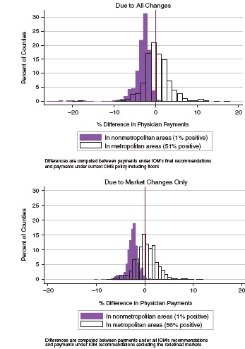
FIGURE 2-3 Distribution of payment effects of IOM committee recommendations on the GPCIs.
NOTE: CMS = Centers for Medicare & Medicaid Services; GPCI = geographic practice cost index; IOM = Institute of Medicine.
SOURCE: RTI simulations.
lower-wage rural and higher-wage urban areas into a single locality. To the extent that the areas do not represent integrated markets, this artificially raises index values in lower-wage areas above what they would be if markets were more locally defined.
The effects of the policy and data-related changes recommended by the committee are more limited than the effects of the market redefinition. Eliminating index floors has a negative impact on payments but only in a small number of areas, while changes to the GPCI data (including adding the benefits index) and the market smoothing adjustments by themselves have a relatively modest impact.11 Committee recommendations for the GPCIs that are not related to redefined markets do not appear to have a systematic redistribution effect by rural or regional location.
Looking at the distribution of payments due to all changes, the counties with the largest total estimated payment reductions (from 15 to 26 percent) are all in Alaska, but these changes reflect the impact of removing the 1.5 Alaska work GPCI rather than the market change. Removing the GPCI floor of 1.0 in frontier states also magnifies the effects of market-related changes in rural counties for the four states affected by the frontier state policy.
Among metropolitan counties, roughly half would see a reduction in payment rates and half would see an increase. If all of the committee’s GPCI recommendations were implemented, the aggregate payment effect across metropolitan counties would be an increase of less than one half of 1 percent. This contrasts with the impact among nonmetropolitan counties, where the aggregate payment effect would be a reduction of nearly 3 percent.
Effects in Statewide vs. Nonstatewide Payment Localities
There are states where the current payment localities are statewide. In these states, the effect of moving from payment localities to CBSA markets is predictable as higher-cost metropolitan areas are separated from the lower-cost nonmetropolitan areas.
There are 55 payment localities that represent parts of states, of which 14 are “rest-of-state” localities and 41 are specifically identified urban localities. The effects of market redefinition are still significant in these localities. In part this is because the urban localities are often larger than defined metropolitan CBSAs, either encompassing multiple metropolitan areas or encompassing outlying rural counties.
There are also instances where the urban localities do not include counties that are identified as part of metropolitan CBSAs. As a consequence, county-level effects of the market redefinition are not as predictable in the nonstatewide localities. A larger urban locality that encompasses two metropolitan areas will be separated into two metropolitan markets, with the result that one will see increased rates and another will see a decrease. A nonmetropolitan county currently grouped in an urban locality may see a large decrease in rates from the market redefinition, but a metropolitan county currently excluded from the urban locality could see substantially higher rates.
______________
11 Cross-market worker commuting patterns resulted in smoothing adjustments to index values in nearly three-fourths of all counties, but the adjustments are small for all but a few areas. Commuter-based smoothing was applied to the wage and purchased services component of the PE-GPCI as well as to the physician work GPCI. It had the strongest impact on the wage component index (adjustment factors ranging from 0.9 to 1.2). Factors greater than 1.10 occurred in only 14 counties, and there was only one county with a factor of 0.90. Smoothing factors for the physician work GPCI ranged from 0.97 to 1.06. With respect to the effects of incorporating a benefits index, Puerto Rico is the only area where this resulted in a substantial reduction in the wage component index. A review of the data indicates that this could be due to underreporting of benefits on the Medicare Cost Report.
For rural counties, the average payment effect from moving to CBSA markets in the statewide payment localities are very similar to those in nonstatewide localities, as shown in Figure 2-4.
Isolating the Effects of Removing Index Floors
The PE-GPCI values as computed under the committee’s recommendations do not include any of the existing frontier state floors of 1.00, and they do not include the physician work floor of 1.5 for all of Alaska. While the committee is not opposed to the idea of targeting special payments or bonuses to create incentives to improve the supply of primary care practitioners, it has taken a position against making special adjustments available based solely on geographic location rather than demonstrated need.
Eliminating the frontier state floors reduces physician payments in four of the five eligible states. (In Nevada, the PE-GPCI is already higher than 1.0 due to the strong influence of Reno within the statewide payment locality.) In Montana, North Dakota, South Dakota, and Wyoming, the CMS PE-GPCIs without the frontier floor are 10 to 12 percent lower than they are with the floors, which would translate into payment reductions of 4 to 5 percent in the absence of any other changes to the GPCIs. In aggregate, physician payments to the remaining four frontier states under the committee’s proposed GPCIs are also estimated to be 5 percent lower than payments under current policy.
In Alaska, current policy sets the physician work GPCI at 1.5. Without this limit, the work GPCI would be 1.015 for the statewide Alaska locality, or 32.3 percent lower. In the absence
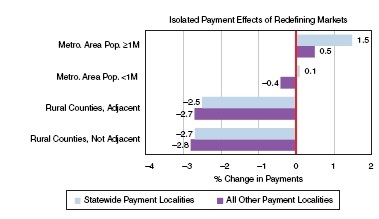
NOTE: Values plotted are the percent difference between payments computed using geographic practice cost indexes with all Institute of Medicine committee recommendations vs. payments computed under current Centers for Medicare & Medicaid Services policy.
SOURCE: RTI simulations.
of any other changes to the GPCIs, eliminating the 1.5 floor would translate to a 19 percent reduction in the GAF (from 1.257 to 1.023) and an estimated 20 percent reduction in payments. In aggregate, physician payments in the state of Alaska under the committee’s proposed GPCIs are also estimated to be 19 percent lower than payments under current policy.
Physician Payments Effects by Geographic and Demographic Subgroups
Technical corrections to GPCIs are intended to improve accuracy and have not been motivated by any a priori objective with respect to the rural—urban distribution of Medicare payments. Nevertheless, the negative effect of the committee’s recommendations on payments to rural areas suggests that correcting the GPCIs could have a disproportionate effect on vulnerable or underserved populations. The frontier floors came into effect very recently, in 2011, and it is not clear whether they have had much of an effect yet or what would happen to the health of underserved or vulnerable populations if they were withdrawn.
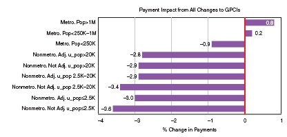
The remainder of this section discusses estimates of the overall payment effects of the committee’s recommendations across counties grouped by key geographic, demographic, and health care shortage area measures. Figure 2-5 shows the payment effects on counties grouped by the U.S. Department of Agriculture’s (USDA’s) Rural−Urban Continuum Codes (RUCCs).12 Payments in counties in large metropolitan areas (population ≥1 million) increase by 0.8 percent, while payments to those in metropolitan areas of 250,000 to 1 million increase only 0.2 percent, and those to metropolitan areas with populations less than 250,000 decrease 0.9 percent. Across the six categories of nonmetropolitan counties, payments decrease somewhat more for those with the smallest urbanized populations.
Many measures of population demographics and health care supply are correlated with rurality. Thus, this differential impact on very rural areas is also reflected in differential impact on other measures. For example, payments in counties ranked in the bottom quartile of median household income (mostly rural) are estimated to decline by 2.6 percent, while those to counties in the highest quartile (mostly urban) show a marginal increase. Payments in counties with the highest proportion of minority populations (which also tend to be in larger urban areas) are virtually unchanged, while payments in counties ranking in the lowest quartile by percent minority population show a decline of 2 percent.
Physician Payment Effects by Health Professional Shortage Areas (HPSAs)
Primary care shortage areas are a key construct for the committee’s deliberations in addressing its mandate to consider the impact of geographic payment adjusters on access to care. It was therefore important to the committee to analyze the payment impact of its recommendations using valid and up-to-date measures of underservice. The Health Resources and Services Administration’s (HRSA’s) HPSAs are identified both by geography (by census division or county) and by institution (for example, specific safety-net provider catchment areas). To implement the primary care bonus payment provisions of the Patient Protection and Affordable Care Act, CMS uses a file that maps HRSA’s primary care service shortage areas to specific ZIP codes, and then pays the bonus to qualifying practitioners for services delivered in that ZIP code.
______________
12 RUCCs group the metropolitan counties according to the size of the total population in the areas. The nonmetropolitan counties are classified by the size of the “urbanized” population (which can be in multiple towns) and by adjacency to a metropolitan area. RUCCs were last updated in 2003.
SOURCE: RTI simulations.
The committee used HPSAs as a measure of access and underservice for several reasons. HPSAs are a recognized standard in workforce research in that they are the official national designation of shortage areas, and they are also being used for a new incentive payment program for primary care services and general surgery in underserved areas from 2011 to 2015, as described in Chapter 4. There are some recognized drawbacks to using HPSAs, including their degree of currency and accuracy as designated shortage areas compared with other nondesignated areas, the degree to which they affect access given that patients travel outside the HPSA to seek health care, their high practitioner vacancy rates and varying appeal to practitioners as practice locations, and the fundamental differences in access problems between rural and urban HPSAs. However, the committee viewed HPSAs as the generally accepted approach for its deliberations and its payment simulations.
The estimated payment effects for this study are computed at a county level, but linking the variously defined shortage areas to counties is not a straightforward task. HRSA’s Area Resource File provides a three-level county shortage area indicator, where counties are identified only as a “full” shortage county, a “partial” shortage county, or “not a shortage county.”13 Many counties are identified as “partial,” particularly in metropolitan areas, and linking the payment impact to this indicator did not provide a strong enough base to evaluate the impact of the committee’s recommendations on actual shortage area populations.
To provide a county shortage variable with more information, a new indicator was constructed based on the CMS ZIP codes for the primary care bonus awards in 2012, using a commercial file that is organized by ZIP code/county subareas.14 The next step was to compute
______________
13 HPSA designations are discussed in more detail in Box 3-1 in Chapter 3.
14 Roughly one in five ZIP codes crosses over more than one county. The database also provides a statistic to use as an approximate population weight for each subarea, allowing us to develop a measure of how much of any one county’s population is included in the bonus-eligible ZIP codes. Further detail on this computation is provided in Appendix A-1.
an estimate of the proportion of each county’s population located in the areas covered by the primary care bonus payments, review the distribution of this measure, and then construct a new five-level county indicator. Counties are identified as “nonshortage” if the county proportion of the estimated population in bonus areas is 0 percent; one of three levels of “partial shortage” if the county proportion in bonus areas is from 1 to 20 percent, 20 to 80 percent, or 80 to 99 percent; and “full shortage” if the estimated population in bonus areas is 100 percent. The results are shown below in Table 2-5.
Table 2-6 shows the combined payment effects of all proposed GPCI changes stratified by this new county HPSA variable. To identify any association between estimated payment effects
TABLE 2-5 Distribution of Counties and Beneficiaries Across Newly Constructed HPSA Categories
| New HPSA County Categorical Variable | Number of Counties | Percent of Counties | Percent of Population* |
| Nonshortage counties | 1.216 | 38% | 44% |
| Partial shortage counties: Low ≤20% | 1.065 | 33% | 50% |
| Medium 20 to 80% | 140 | 4% | 2% |
| High 80 to 99% | 549 | 17% | 1% |
| Full shortage counties | 255 | 7% | 1% |
NOTE: HPSA = Health Professional Shortage Area.
* Percent of 2009 population living in counties assigned to this row.
SOURCE: RTI analysis of CMS Bonus Area Files.
| Metropolitan | Nonmetropolitan | |||||
| HPSA County Status, by Estimated Share of County Population in CMS Primary Care Bonus Areas | Percent Difference in Paymentsa | Share of Part B Enrolleesb | Share of Total Primary Care RVUsc | Percent Difference in Paymentsa | Share of Part B Enrolleesb | Share of Total Primary Care RVUsc |
| Non HPSA: 0% | +0.7% | 0.365 | 0.384 | -2.8% | 0.089 | 0.063 |
| Partial HPSA: ≤20 percent | +0.1% | 0.369 | 0.437 | -3.0% | 0.096 | 0.075 |
| 20 to SO percent | -0.8% | 0.011 | 0.008 | -2.5% | 0.010 | 0.005 |
| 80 to<100 percent | -1.3% | 0.012 | 0.005 | -3.0% | 0.032 | 0.013 |
| Full HPSA: 100% | -1.4% | 0.004 | 0.003 | -3.7% | 0.012 | 0.006 |
| All counties | .0.4% | 0762 | 0.836 | -2.9% | 0.238 | 0.164 |
NOTE: CMS = Centers for Medicare & Medicaid Services; HPSA = Health Professional Shortage Area; RVU = relative value unit.
aDefined as difference between payments estimated with GPCIs computed using all of the committee’s recommendations, relative to payments estimated under current CMS policy, including all floors.
bShare of Medicare beneficiaries enrolled in Part B fee-for-service program, from calendar 2009 (most recent county data available for download as of January 2012).
cShare of national total Part B RVUS billed in 2010 by physicians identified as internists, geriatricians, family practitioners and pediatricians, plus RVUs billed by nurse practitioners and physician assistants.
SOURCE: RTI simulations.
and HPSA status that is independent of the rural-urban differentials already noted, the table also stratifies by metropolitan status. This table also includes columns showing the share of Part B enrollees in these county subgroups and the share of total primary care RVUs.
From this table there appear to be larger reductions in payments in the counties with HPSA shortage areas, but the number of counties in the higher shortage area categories is very small.15 Overall, in metropolitan areas, the percent decrease grows smaller as the percent of the populations living in an HPSA increases, while in nonmetropolitan areas, the percentage difference does not vary with the HPSA measure. Specifically, payments to physicians in metropolitan non-HPSA counties are estimated to increase by 0.7 percent, while payments to physicians in metropolitan full HPSA counties (only 31 counties) are estimated to decrease by 1.4 percent. Payments to physicians in nonmetropolitan counties are estimated to decrease by 2.8 percent while payments to physicians in full HPSAs (224 counties) are estimated to decrease by 3.7 percent. It is also worth noting that despite their constrained resources, full HPSAs in nonmetropolitan areas shoulder the burden of three times more beneficiaries than full HPSAs in metropolitan areas and twice as many primary care RVUs.
The committee recognizes the importance of ensuring adequate Medicare funding to physician practices in both urban and rural shortage areas. The committee’s Phase I principles state clearly that GPCIs should be used only to adjust for input cost differences, but reductions in payments to any shortage area potentially pose a policy problem that may need to be offset through other policy adjustments or programmatic interventions. For example, CMS could consider increasing the bonus payment for primary care practitioners in the primary care bonus ZIP codes, if those ZIP codes are located in a county where the GPCI changes result in a payment reduction.16 To illustrate how this might work, Figure 2-6 is a county-level map for the state of North Dakota. Each county is shaded according to its shortage area category, from the lightest areas (no shortage) to the darkest areas (full shortage). Additional cross-hatching identifies metropolitan counties. The numbers shown on each county are the percent change in payments that are estimated as a result of the committee’s recommendations.
The Medicare Part B primary care bonus is currently a 10 percent increase for any services delivered by an eligible provider in an eligible ZIP code. For purposes of illustration, suppose that CMS modified this to say that the bonus would be increased to (10 + x) percent for any service delivered in a bonus-eligible ZIP code where the revised GAF is less than the current GAF. North Dakota is one of the five frontier states, and the proposed revised GAF is lower than the current GAF for all of its counties. There are 11 counties identified as “full shortage” counties (all rural), and combined they account for 1.4 percent of all billed RVUs in the state. The estimated payment impact of the committee’s recommendations ranges from −4.5 to −9.6 percent, and all eligible primary care providers in these counties would be eligible for an offsetting increase to the bonus. There are 16 counties where less than 20 percent of the population is estimated to live in primary care bonus areas, three of which are metropolitan. These 16 counties account for 95 percent of all RVUs billed in the state, and the estimated payment impact of the committee’s recommendations ranges from -2.7 to -7.9 percent. An offsetting increase to their bonus
______________
15 We tested for significant differences across these groups using separate RVU-weighted regressions for metropolitan and nonmetropolitan counties. Some but not all of the differences in payment impact across HPSA county subgroups were significant when tested against payment impact in non-HPSA counties in both regressions, although there was no pattern of increasing impact by level of shortage.
16 Section 413 in the Medicare Modernization Act of 2003 stipulates many of the details surrounding the current bonus payments. Adjustments to these bonus payments may therefore require congressional action. See http://www.cms.gov/Medicare/Medicare-Fee-for-Service-payment/HPSAPSAPhysicianBonuses/downloads//Overview.pdf.
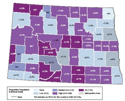
FIGURE 2-6 Sample state map identifying payment impact and HPSA status by county (North Dakota: Physician payment impact vs. HPSA county designations, by estimated proportion of population living in CMS primary care bonus areas).
NOTE: CMS = Centers for Medicare & Medicaid Services; HPSA = Health Professional Shortage Area; RVU = relative value unit.
SOURCE: RTI analysis of ZIP codes eligible for CMS primary care bonus payments in 2012.
payments would apply only to practitioners located in the bonus ZIP codes, while the other practitioners in the counties would be subject to the full reductions.
There are three key advantages to this type of approach over a market-wide adjustment, such as applying an index floor. The most important is that special payment bonuses remain targeted to areas in need—in this case, to geographic primary care provider shortage areas, where the purpose of increasing the payments is to encourage more practitioners to locate in these underserved areas. In this example, a small number of areas in Grand Forks, Fargo, and Bismarck metropolitan areas would receive offsetting bonus payments, but most practices in those metropolitan areas would not.
A second major advantage is that the bonus payments do not have to be funded from reduced payments elsewhere in the system. They represent new money to the system, but new money that is applied to a relatively small proportion of billed RVUs. The frontier floors were not made budget-neutral by Congress and therefore also represent new money, but these extra
payments were awarded across the board to all providers in the five states, whether or not the area is experiencing provider shortages.
Finally, a third advantage to this type of approach over something like the frontier floors is that the geographic price indexes remain an accurate (or at least more accurate) reflection of real market-level input price variation.17
Optional Assumptions for the Physician Work GPCI
In its Phase I report, the committee did not recommend a change in the use of proxy professions as a basis for the physician work GPCI, but it did recommend that further empirical analysis be conducted to test the correlation between the proxy professions and RVU-adjusted physician income. Findings from these recommended analyses would then be used to review the current policy of using one-quarter of the proxy work adjustment as the physician work GPCI.
All of the simulations discussed thus far have incorporated a continuation of the one-quarter work GPCI. This section addresses the impact of the work adjustment by simulating payments at the upper (100 percent) and lower (0 percent) bounds of the proxy index. Although the effect could be estimated as a simple proportional change, a full simulation was preferable because the share of work RVUs to total RVUs varies by county, and the correlation between the work GPCI and other GPCIs also varies by county.
Eliminating the physician work adjustment altogether clearly reduces the impact of the committee’s other recommendations on all counties, reducing the slight estimated payment increase in metropolitan areas from +0.4 down to +0.1 percent, and reducing the estimated payment decrease in nonmetropolitan counties from −2.9 to −1.1 percent. Likewise, applying the full work adjustment increases the impact of the committee’s other recommendations on all counties, raising the estimated payment increase in metropolitan areas from +0.4 to +1.1 percent, and the estimated payment decrease in nonmetropolitan counties from −2.9 to −8.4 percent.
The differential impact of the committee’s GPCI recommendations would be seen primarily between urban and rural county designations rather than low-shortage and high-shortage area designations. The extent to which an area would be disadvantaged or benefit from the recommendations, once implemented, is partially dependent on the percentage work adjustment. The least impact would be felt with a 0 percent adjustment and the most with a 100 percent adjustment, with the impact of a 25 percent adjustment, the current level, falling within the two extremes.
This section provides examples to illustrate some of the ways in which selected providers would experience significant changes as a result of the committee’s recommendations. In the case of the GPCIs, the examples focus on how and why the payments differ under the CBSA markets as compared to payment localities. The first two are individual counties with large negative or positive payment effects, and the third describes statewide effects in Minnesota.
______________
17 Notably, most of the policy adjustments, such as the frontier floors, the work GPCI floor in Alaska, and the rural floor for the HWI are congressional mandates. Standard reclassification rules were regulatory, originally contained in the enabling regulations for the Medicare Geographic Classification Review Board in the late 1980s, but over the years Congress has adopted various mandated changes. Thus, replacing the policy adjustments and reclassification rules would require congressional action.
The specific areas are chosen to illustrate how different the impact of market redefinition can be when the current payment localities cross multiple rural-urban designations.
In the case of the HWI, the examples focus on the effect of removing the rural floor on metropolitan areas in California, Massachusetts, and Ohio. These examples consider the degree to which these changes may be due to the rural floor distorting the accuracy of the HWI versus the switch from using hospital-reported occupationally adjusted wage data to BLS wage data. Finally, this section also gives examples of three of the largest adjustments that are made to the HWI as a result of applying the outmigration commuter smoothing method.
On the GPCI side, the largest decrease in payments attributable to the market redefinition is in Monroe, Florida, which is currently part of the Miami payment locality. Under the CBSA classification, however, it is a single-county micropolitan area south and west of Miami that incorporates the Florida Keys, the Big Cypress National Preserve, and parts of the Everglades. Because of the distance to the main population center (Key West), there is relatively little commuting to Miami and consequently only a small bump up in the CBSA indexes from smoothing adjustments (+0.4 percent for the wage component of the PE-GPCI, and +0.1 percent for the overall GAF). From the combined effects of market and smoothing adjustments, payments in Monroe, Florida, are estimated to decline by 10.4 percent.
The largest increase from the market redefinition is in Jefferson, West Virginia. This county is currently part of the West Virginia statewide payment locality, and West Virginia has historically had very low relative wages. Under the current CBSA designations, however, Jefferson is considered part of the Washington, DC—Arlington—Alexandria metropolitan area—where relative prices are considerably higher. Although the county is included in the DC-Arlington CBSA because of its strong commuting pattern into the area, later commuting data also indicate that more than a quarter of Jefferson County’s resident health care workers have jobs in the adjacent Hagerstown and Winchester metropolitan areas, where the relative wages are not as high as those in the DC metro area. The estimated payment increase due to market reassignment would have been even higher if we had not applied smoothing adjustments (a negative 2.8 percent adjustment to the wage component of the PE-GPCI, and -1.8 percent for the overall GAF). From the combined effects of market and smoothing adjustments, payments in Jefferson, West Virginia, are estimated to increase by 12.0 percent.
Many of the counties with the largest payment reductions resulting from market redefinition are in Minnesota, which is currently under a statewide payment locality. Taking all of the committee’s recommendations into account, the estimated payments for the state are about 1.6 percent higher than under current policy. If we isolate just the effect of the market redefinitions, state payments in aggregate are less than half of 1 percent higher under the CBSA markets. Part B services in this state are highly concentrated in a few urban areas, however, and separating rural from urban areas tends to have a modest impact on the urban areas but a larger one on the rural counties. There are 87 counties in Minnesota, 23 of which are included in eight metropolitan areas. The Minneapolis—St. Paul area accounts for more than half the RVUs generated in this state, and their payments under the redefined markets are 2 percent higher than they would be under a statewide locality. In the Rochester area, which accounts for 18 percent of the state’s RVUs, payments under the redefined markets are 1.6 percent higher. For the other six metropolitan areas in the state, however, payments are lower, with aggregate decreases ranging from 2.1 to 6.3 percent.
Aggregate payments to nonmetropolitan counties under the CBSA markets are 5.6 percent lower than they are under a statewide locality, and would have been 6.5 percent lower had it
not been for smoothing adjustments based on commuting patterns into the metro areas. Across rural counties, the payment effects range from −3 to −7 percent. Commuter-based smoothing works to the advantage of 29 out of 64 rural counties; in Goodhue County, for example (just south of St. Paul) smoothing increased the PE-GPCI by 11.6 percent and the overall GAF by 3.2 percent. Fillmore, Mower, and Winona counties (surrounding the Rochester metro area) all have similarly large smoothing adjustments. There are only 10 rural counties where smoothing adjustments are negative, but most of these are state border counties to the east, and the adjustments are generally small (less than half a percent on the GAF).
On the HWI side, some of the largest decreases in payments attributable to removing the rural floor can be seen in the states of California, Massachusetts, and Ohio. Massachusetts is a unique example of the rural floor as a result of the “Nantucket effect.” Prior to 2012, the Nantucket Cottage Hospital was classified as a critical access hospital and therefore did not figure into the computations for the states’ IPPS HWI rural floor. However, as a result of being acquired by a large health system, the Nantucket Cottage Hospital converted to IPPS status, becoming the only rural IPPS hospital in the state of Massachusetts. This change resulted in the rural floor wage index being applied to 60 urban hospitals in the state of Massachusetts, increasing wage indexes for these hospitals from an average of 1.16 in FY 2011 to 1.35 in FY 2012.18 It is therefore not surprising that the isolated effect of removing the rural floor in Massachusetts would result in a 9–29 percent decrease in the HWI for urban hospitals across the state. For the majority of metropolitan areas in Massachusetts, the original occupationally adjusted HWIs that are based on wage data reported from hospitals only differ from the committee’s recommended wage indexes using BLS data by a few percentage points compared to the 19–29 percent difference between the pre- and postrural floor occupationally adjusted indexes. This underscores the importance of removing the rural floor in order to improve the accuracy of the HWIs for hospitals in Massachusetts.
While all of the metropolitan areas in Massachusetts are significantly affected by the rural floor, the impact of removing the rural floor would be more moderate in most states. In the state of Ohio, 11 of the 16 metropolitan areas would actually experience an increase in their HWI as a result of replacing the hospital reported occupationally adjusted wage data with wage indexes based on benefits-adjusted BLS data. Four metropolitan areas in Ohio would experience modest decreases of 0.1-2.6 percent in their HWIs as a result of removing the rural floor, while the metropolitan area of Wheeling would experience a larger decrease of 14.1 percent. Notably, in Ohio, three of the metropolitan areas cross state lines, which currently results in some of the counties benefiting from the rural floor more than others within the same MSA. This is likely the case in Wheeling, which sits right on the border of Ohio and West Virginia. By removing the rural floor, the HWI for counties in Wheeling that sit in Ohio will more accurately reflect local wages in both states, rather than just the rural floor in Ohio.
In the state of California, 26 of the 28 metropolitan areas would experience a decrease of between 2 and 20 percent in their HWIs as a result of moving from the occupationally adjusted HWI with the rural floor to the IOM committee’s benefits-adjusted wage index based on BLS data. However, the decrease in the HWI value is attributable to the removal of the rural floor (versus the switch to BLS data with the benefit adjustment) in only half of these cases, as evidenced by the relatively large percentage differences between the committee’s index using BLS data and the original occupationally adjusted index prior to applying the floor in these
______________
18 MedPAC, June 17, 2011, letter to CMS. http://www.medpac.gov/documents/06172011_FY12IPPS_MedPAC_COMMENT.pdf.
markets. This is in contrast to Massachusetts, where the decrease in HWI was clearly caused by the removal of the rural floor for the vast majority of the metropolitan markets.
The effect of removing the rural floor is more dramatic in some states than others as a result of the differing degrees of inaccuracy that result from the current policy. In addition, the effect of applying the outmigration commuter smoothing adjustment is also larger in some counties than others. In the case of Yuba County, California, approximately three-quarters of the health care workers in that county commute to other counties that are in the same metropolitan statistical area, Yuba City. However, the other one-quarter of health care workers commute to counties in other metropolitan statistical areas (namely, the MSAs of Chico and Sacramento—Arden—Arcade—Roseville) that have higher benefits-adjusted indexes based on BLS data. The result is that the HWI for the one hospital in Yuba County, California, increases from 1.046 to 1.107 as a result of applying the smoothing adjustment, representing a 5.8 percent increase in payments. Thus, this is an example of where the commuter-adjustment method improves the accuracy of HWIs in areas where workers may commute across MSAs.
Similarly, the 39 hospitals in Monroe County, Pennsylvania, also experience a significant increase in their HWI of 9.5 percent as a result of the commuter smoothing adjustment. Two- thirds of health care workers commute to counties inside the same rest-of-state area in Pennsylvania. However, the other one-third of health care workers commute to MSAs that have significantly higher HWIs, including the relatively high wage area of New York—White Plains—Wayne, an MSA that crosses the New York and New Jersey borders. Thus, this is an example of an area in which the commuter smoothing adjustment appropriately results in an increase to the HWI for hospitals in a relatively rural area that must compete with hospitals in higher-wage metropolitan areas.
Finally, it is important to give an example of an area in which hospitals experience a decrease in their HWIs as a result of the outmigration commuter adjustment method. The majority of the decreases in HWIs as a result of health care workers commuting to other counties occur in counties where there are not any hospitals. This is not surprising, given that fewer jobs are likely to be available for health care workers in a county that has no hospital, forcing them to migrate to other areas. Tazewell County, Virginia, is an example of a county that would experience a decrease in its HWI, albeit a relatively small decrease of 1.6 percent. This decrease is the result of 22.7 percent of the health care workers in Tazewell County commuting from the rest-of-state area Virginia to a county in the rest-of-state area of West Virginia.
In Box 2-5, two examples of special circumstances are described in terms of the physician payment simulations. The first is the state of Alaska, which would experience the largest reductions in payments if the committee’s recommendations were fully implemented as a result of the removal of the 1.5 work floor. The second example is Puerto Rico, whose reduced payments from the simulations are due primarily to the way missing data were handled in the simulations. Both examples would warrant additional consideration if the recommended changes were to be implemented.
This chapter highlights the impact that the committee’s recommendations would have on the HWI and the GPCI. The changes recommended in the Phase I report were made to improve the technical accuracy of the price adjusters as measures of market-level variation in health care input prices.
The committee believes that increases in payments reflect evidence that current CMS prices
BOX 2-5
Further Narrative on Alaska and Puerto Rico
Under the committee’s more technically accurate indexes, Alaska would experience the largest reductions in payments, with reductions of approximately 20 percent across CBSAs and the rest-of-state area. The implications of these reductions warrant further consideration of the issues surrounding the GAFs for this state. In addition, Puerto Rico is also a unique case. While its changes in payments are more modest (0.47 to −3.97 percent across CBSA areas), it is important to acknowledge concerns about missing data in this territory.
In Alaska, the final GAFs would decrease following the committee’s recommendations as a result of the 1.5 work floor removal. The committee believes the work floor was an inaccurate reflection of the geographic input cost differentials in physician work in Alaska. Instead, moving to MSA-based payment localities would assign an appropriately higher GAF to metropolitan areas such as Anchorage, Fairbanks, and Matanuska-Susitna, relative to the rest of the state. Moreover, even with the removal of the work floor, all of the new payment localities in Alaska under the MSA-based system would still retain GAFs of over 1, reflecting the higher input costs in Alaska, relative to the rest of the nation.
While the GAFs under the committee’s recommendations would be more accurate, the committee acknowledges the current access problem in Alaska and supports other policy mechanisms to help address this problem. A recent report interviewed Alaska physicians who had not accepted new Medicare patients in the previous year, and found that less than 20 percent of primary care physicians in Anchorage, Fairbanks, and Matanuska-Susitna were accepting new Medicare patients (Frazier and Foster, 2009). Primary care physicians in rural areas and medical specialists were more willing to see new Medicare patients. This report goes on to point to the reimbursement difference between Medicare and private insurance for physician services, concluding that primary care physicians in Alaska and Fairbanks are declining new Medicare patients because Medicare reimbursement is only 66 percent of private reimbursement. Notably, they also acknowledge that this differential in Alaska is the same as the national average, and portends a growing access problem for Medicare beneficiaries nationwide. While payment differentials between Medicare
have been underpaying providers by not accurately accounting for exogenous factor prices. Conversely, reductions in payments are interpreted as evidence that providers have been overcompensated for services delivered. The committee also acknowledges that it is important to understand the implications that these changes may have on access to care. As part of this task, this chapter therefore also assesses the effects the committee’s recommendations could have on health care shortage areas or at-risk populations and providers.
Key Findings from Hospital Payment Simulations
1. If the more technically accurate wage index were implemented, the change in payments would be between −5 and +5 percent for discharges in 88 percent of hospitals.
2. The most substantial differences in payments under the index as recommended by the committee as compared to payments under current CMS policy are the result of eliminating policy adjustments, such as the various exceptions, market reclassifications, and floors, rather than the result of technical corrections to improve accuracy.
and private insurers have significant policy implications, the committee does not believe that GAFs are the appropriate tool for addressing this. Rather, the purpose of the GAFs is to adjust for geographic differences in input costs across areas, but it is not intended to make Medicare competitive with private health insurance reimbursement levels. If there is concern that Medicare does not pay enough relative to private insurance, this may be because private insurance is overpaying, or because Medicare is underpaying, which reflects an issue with the relative value unit system and/or the payment updates (i.e., increases/decreases).
Unlike in Alaska, where the large reduction in payments results from the committee’s recommendation to remove the work GPCI floor, in Puerto Rico payment changes result from the committee’s treatment of missing data. Specifically, the committee deals with missing data by renormalizing, which assigns national weights to the occupations for which there are data, ensuring that the weights sum to one in each area. This method differs from the CMS’ current practice of replacing missing data with national medians. Out of the top 25 occupations in the physician office industry, wage data across areas are only available for between 11 and 15 occupations in Puerto Rico. The committee’s process of renormalizing assigns all of the weight to occupations for which local wage data do exist, thereby reflecting the weighted average wages of that area’s occupation mix. Conversely, CMS’s current method of assigning national medians to occupations with missing data holds the occupation mix constant, but biases the area wage index toward the national average. In the case of Puerto Rico, the large wage differences between areas in Puerto Rico and the national average therefore cause an inaccurately high wage index, resulting in a decrease when reassigning all of the weights in the index to occupations for which data exist in Puerto Rico.
In addition, Puerto Rico is the only area that experiences a substantial reduction in wage portion of the practice expense index as a result of the benefits add-on. For example, the isolated effect of the benefit add-on to the practice expense GPCI in Guanica Mun County, Puerto Rico, is −10.8 percent. This is likely also due to data limitations, reflecting the potential underreporting of benefits on the Medicare Cost Report. Thus, although the committee believes that its method of renormalizing is a more accurate way to treat missing data than assigning inflated national medians, concerns about missing wage and benefits data in Puerto Rico warrant further attention by CMS to ensure accurate indexes.
a. The largest negative effect on payments in metropolitan areas is due to the elimination of state rural floors for metropolitan areas in states where the index for the rural area is higher than an index for a metropolitan area. For the majority of these areas the committee’s revised index for metropolitan areas is lower than the index under the current system with the rural floor.
b. Commuter-based smoothing adjustments have a modest effect on the HWI in the great majority of counties (99 percent of the HWIs after smoothing are between 0.99 and 1.04), but smoothing serves to partially offset the effects of eliminating reclassifications.
3. A HWI based on BLS data yields generally higher relative wages in rural areas, as compared to an index based on IPPS hospital data.
4. In general, relative wages computed from benefits-adjusted BLS data are not substantively different from relative wages computed from CMS hospital data. There are notable exceptions, however, in markets where few hospitals contribute to that market’s CMS index.
5. Payments to rural referral centers are slightly lower under the index proposed by the committee. Payments to other rural hospitals with special payment status are generally higher (roughly 1 percent), except for those located in frontier states.
6. The committee found no specific types of hospitals (for example, by teaching status, disproportionate share status, size, or region) that appeared to be disproportionately advantaged or disadvantaged by moving to a more technically accurate index.
Key Findings from Physician Payment Simulations
1. If the more technically accurate GPCIs were implemented, the changes in payments would be between −5 and +5 percent in counties where 96 percent of RVUs are billed. Most of the redistribution would be from rural to urban areas and from small urban to large urban areas.
2. The most important intervention to improve accuracy of physician payment adjusters is the move from current payment localities to CBSA market areas.
3. GPCIs computed under CBSA markets yield lower relative wages in rural areas, as compared to GPCIs computed under the larger payment localities.
4. Commuter-based smoothing adjustments have a modest effect on the GPCIs for the great majority of counties (99 percent of the wage component of the PE-GPCIs after smoothing are between 0.98 and 1.07), but smoothing serves to partially offset the impact of changing to CBSA markets in rural counties that are adjacent to metropolitan areas.
5. Because many rural areas are also HPSAs, physician payments under the committee’s proposed indexes are reduced in most of the rural primary care shortage areas that are currently eligible for Medicare primary bonus payments. Among medium, high, or full primary care shortage counties in rural areas, estimated payment changes range from a reduction of 26 percent to an increase of 1.7 percent.
6. The impact of the changes would vary primarily between metropolitan and nonmetropolitan county designations rather than across HPSA designations. The positive effects on metropolitan counties and negative effects on nonmetropolitan counties would be reduced with a 0 percent adjustment for physician work and increased with a 100 percent work adjustment. The impact of a 25 percent adjustment, the current level, would fall within the two extremes.
7. Under the committee’s more technically accurate indexes, areas with the highest reductions in payments would be the frontier states, with Alaska experiencing the largest reduction.
Frazier, R., and M. Foster. March 2009. How hard is it for Alaska’s Medicare patients to find family doctors? UA Research Summary No. 14. Institute of Social and Economic Research, University of Alaska. http://www.iser.uaa.alaska.edu/Publications/researchsumm/UA_RS14.pdf (accessed June 20, 2011).
IOM (Institute of Medicine). 2011. Geographic adjustment in Medicare payment: Phase I: Improving accuracy. Washington, DC: The National Academies Press.


