
Appendix D
Statistical Calibration
In the following, the ordinary least squares (OLS) and the weighted least squares (WLS) approaches to estimating the calibration function and related interval are reviewed.
OLS ESTIMATION1
As preparation for the following discussion, consider the relationship between response signal y and spiking concentration x in the region of the detection and quantification limits as a linear function of the form
![]()
where ![]() is a random variable that describes the deviations from the regression line, distributed with mean 0 and constant variance
is a random variable that describes the deviations from the regression line, distributed with mean 0 and constant variance ![]() . The assumption of constant variance is not critical to this approach and will be relaxed in a later section; however, it is useful to simplify the initial exposition. The sample regression coefficient
. The assumption of constant variance is not critical to this approach and will be relaxed in a later section; however, it is useful to simplify the initial exposition. The sample regression coefficient
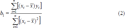
provides an estimate of the population parameter β1 (i.e., the slope of the calibration function). The sample intercept
![]()
provides an estimate of the population parameter β0 (i.e., the intercept of the calibration function, which describes the mean instrument response or measured concentration when
![]()
1This section is adapted from Gibbons, 1995.
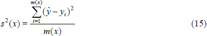
true concentration x = 0). An unbiased sample estimate of ![]() (i.e., the variance of deviations from the population regression line) is given by
(i.e., the variance of deviations from the population regression line) is given by
![]()
where ![]() .
.
WLS ESTIMATION2
When variance is not constant, as is typically the case in the calibration setting, then the previous OLS solution for constant or “homoscedastic” errors no longer applies. There are several approaches to this problem, but in general the most widely accepted approach is to model the variance as a function of true concentration x and to then use the estimated variances as weights in estimating the calibration parameters, which are now denoted as ![]() and
and ![]() .
.
The weighted least squares regression of measured concentration or instrument response (y) on true concentration (x) is denoted by
![]()
where
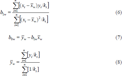
![]()
2This section is adapted from Gibbons and Bhaumik, 2001.
and the weight ![]() is the variance for sample i, which is computed from those samples with true concentration xi = x. The weighted residual variance is
is the variance for sample i, which is computed from those samples with true concentration xi = x. The weighted residual variance is
![]()
ESTIMATING THE WEIGHTS3
When the number of replicates at each concentration is small, as is typically the case, or there are no replicates, the observed variance at each concentration provides a poor estimate of the true population variance. Two better alternatives are to (1) model the observed variance or standard deviation as a function of true concentration or (2) model the sum of squared residuals as a function of concentration. The latter approach can also be performed iteratively, in which improved estimates of β0 and β1 are obtained from weights computed from the current sum of squared residuals on each iteration. These new estimates of β0 and β1 are in turn used to obtain a new set of estimated weights and so forth until convergence. This algorithm is commonly termed “iteratively reweighted least squares.” An essential element of either approach is to identify a plausible model for the variance function. The following sections consider a few models that are particularly well suited to this problem.
Rocke and Lorenzato Model
To measure the true concentration of an analyte (x), the traditional simple linear calibration model, ![]() with the standard normality assumption on errors, is not appropriate, as it fails to explain increasing measurement variation with increasing analyte concentration, which is commonly observed in analytical data. To overcome this situation, one may propose a log linear model, for example,
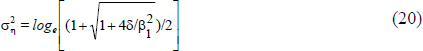
with the standard normality assumption on errors, is not appropriate, as it fails to explain increasing measurement variation with increasing analyte concentration, which is commonly observed in analytical data. To overcome this situation, one may propose a log linear model, for example, ![]() , where η is a normal variable with mean 0 and standard deviation
, where η is a normal variable with mean 0 and standard deviation ![]() . This model also fails to explain near-constant measurement variation of y for low true concentration level x (Rocke and Lorenzato, 1995). To better model the calibration curve, Rocke and Lorenzato (1995) proposed a combined model that has both types of errors:
. This model also fails to explain near-constant measurement variation of y for low true concentration level x (Rocke and Lorenzato, 1995). To better model the calibration curve, Rocke and Lorenzato (1995) proposed a combined model that has both types of errors:
![]()
3This section is adapted from Gibbons and Bhaumik, 2001.
![]()
where y is the r th measurement at the j th concentration level, xjr is the corresponding true concentration, and β0 and β1 are the fixed calibration parameters. In this model, η represents proportional error at higher true concentrations and the ejr ’s are the additive errors that are present primarily at low concentrations. Now assume that η and the ejr ’s are independent and follow normal distributions with means 0 ’s and variances ![]() and
and ![]() , respectively. Data near zero (i.e., x; 0) determine
, respectively. Data near zero (i.e., x; 0) determine ![]() , and data for large concentrations determine
, and data for large concentrations determine ![]() . The model specification also indicates that errors at larger concentrations are lognormally distributed and at low concentrations are normally distributed, which agrees with common experience.
. The model specification also indicates that errors at larger concentrations are lognormally distributed and at low concentrations are normally distributed, which agrees with common experience.
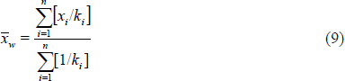
In their original paper, Rocke and Lorenzato (1995) derived the maximum likelihood estimators for their model based on maximizing the likelihood function:
These computations require complex numerical evaluation of the required integrals. Alternatively, Gibbons et al. (1997) and Rocke and Durbin (1998) have described a WLS solution that involves the following algorithm:
1.Use OLS regression to find initial estimates of β0 and β1 by fitting the linear model:
![]()
2.Using the sample standard deviation of the lowest concentration as an estimate for ![]() and the standard deviation of the log of the replicates at the highest concentration as an initial estimate for
and the standard deviation of the log of the replicates at the highest concentration as an initial estimate for ![]() , refit the model in step 1 using WLS with weights equal to
, refit the model in step 1 using WLS with weights equal to
![]()
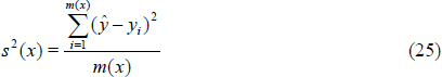
3.Using the new estimates of β0 and β1, compute the predicted response ![]() and standard error of the calibration curve at each concentration x :
and standard error of the calibration curve at each concentration x :
where m(x) is the number of replicates for concentration x
4.Using WLS, fit the variance function:
![]()
where
![]()
and
![]()
using weights:
![]()
5.Compute the new estimates of ![]() and
and
6.Iterate until convergence.
In general, this algorithm will converge to positive values of γ and δ. Note that this algorithm uses WLS to compute the parameters of the calibration curve (β0 and β1) as well as the parameters of the variance function (γ and δ). In this way, the lowest concentrations with the smallest variances provide the greatest weight in the estimation. The net result is to not sacrifice precision in estimating the calibration function and corresponding interval estimates at low levels by including higher concentrations in the analysis. This is quite useful if the interest is in low-level detection and quantification.
Exponential Model
An alternative parameterization of the variance function involves modeling the relationship between σ and x as an exponential function of the following form:
![]()
Although less well theoretically motivated than the Rocke and Lorenzato model, the exponential model provides excellent fit to a wide variety of analytical data (see Gibbons
et al., 1997). The model can be applied either to the observed standard deviations at each concentration or, iteratively, to the sum of squared residuals. For estimating a0 and a1, the traditional approach involves substituting sx for σx and using nonlinear least squares (e.g., Gauss-Newton) or using OLS regression of the natural log transformed observed standard deviation on true concentration (Snedecor and Cochran, 1989). Similarly, WLS can also be used on the regression of ![]() on x using weights
on x using weights
![]()
Linear Model
The linear model has also been used to model the variance function (Currie, 1995). The linear model is of the form
![]()
The primary disadvantage of the linear model is that the small sampling fluctuations in the observed sample variance at each concentration can lead to a negative intercept (i.e., a0 < 0) and negative variance estimates. This can lead to improper detection and quantification limit estimates and corresponding interval estimates. As such, the linear model is generally not recommended for routine use. This is not a problem for either of the two preceding models, which can mimic a linear model if required.
ITERATIVELY REWEIGHTED LEAST SQUARES ESTIMATION
An alternative to modeling the observed variance at each concentration is to model the squared residuals as a function of x, and then to use this estimated variance function to obtain weights that are then used in estimating the regression coefficients. This process is iterated until convergence, hence the term “iteratively reweighted least squares”’ (Carroll and Rupert, 1988). As noted by Neter et al. (1990) the methods of maximum likelihood and weighted least squares lead to the same estimators for linear regression models of the form considered here. The previous example of the WLS estimator for the Rocke and Lorenzato model is an example of iteratively reweighted least squares. The general algorithm is as follows:
1. Use OLS estimation to find initial estimates of β0 and β1 by fitting the linear model
![]()
2. Using the OLS estimates of β00 and β1, compute the predicted response ![]() and the standard error of the calibration curve at each concentration x:
and the standard error of the calibration curve at each concentration x:
where m(x) is the number of replicates for concentration x.
3. Using an appropriate model for the variance function, fit the variance function to the sum of squared residuals:
![]()
4. Using the provisional weights:
![]()
recompute β0 and β1 using WLS.
5. Iterate until convergence.
WLS PREDICTION INTERVALS
For WLS estimates of β0 and β1 the estimated variance for a predicted value ![]() is
is
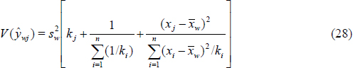
where kj is the estimated variance at concentration xj. An upper (1 -α)100 percent confidence interval for ![]() (i.e., an upper prediction limit for a new measured concentration or instrument response at true concentration xj) is
(i.e., an upper prediction limit for a new measured concentration or instrument response at true concentration xj) is
![]()
where t is the upper (1 -α)100 percent point of Student’s t -distribution on n - 2 degrees of freedom. For example, at x = 0, the upper prediction limit (UPL) is
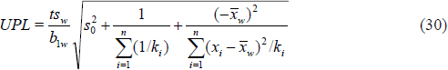
where ![]() is the variance of the measured concentrations or instrument responses for a sample that does not contain the analyte.
is the variance of the measured concentrations or instrument responses for a sample that does not contain the analyte.
CONFIDENCE REGION FOR AN UNKNOWN TRUE CONCENTRATION
In general practice, measured concentrations are reported as if they are true concentrations, without the benefit of an index of uncertainty. There are two problems with this. First, the measured concentration may provide a biased estimate of the true concentration to the extent that ![]() . Second, even in the absence of bias, the measured concentration is only an estimate of the true concentration, and it has a level of uncertainty that is ignored by simply presenting the measured concentration in the absence of a proper uncertainty interval.
. Second, even in the absence of bias, the measured concentration is only an estimate of the true concentration, and it has a level of uncertainty that is ignored by simply presenting the measured concentration in the absence of a proper uncertainty interval.
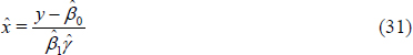
To provide an estimate of true concentration x from measured concentration y for the Rocke and Lorenzato model, compute
Bhaumik and Gibbons (2005) derived the asymptotic variance of ![]() as
as
![]()
where n0 is the number of calibration measurements at or near zero. As expected, the variance of ![]() depends on x and increases with increasing concentration.
depends on x and increases with increasing concentration.
Bhaumik and Gibbons (2005) developed a confidence interval for an unknown true concentration x given a measured concentration y, separately for true concentrations at or near x = 0 and for larger non-zero true concentrations. For a low-level true concentration x0, the (1 -α)100 percent confidence region for x0 is max![]() . To construct a confidence interval for an unknown higher level concentration x, they use a lognormal approximation. Let
. To construct a confidence interval for an unknown higher level concentration x, they use a lognormal approximation. Let
![]()
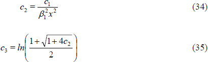
where c3 is the approximate variance of
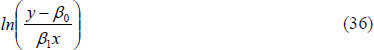
The quantity
![]()
is distributed N(0,1) so that the (1 -α)100 percent confidence region for x0 is obtained by iteratively solving
![]()
In addition to reporting measured concentrations, the point estimate of x and its 95 percent confidence interval should also be routinely reported; it can be used for the purpose of making both detection decisions and comparisons to regulatory standards. If, for example, the lower 95 percent confidence limit is greater than zero, there is 95 percent confidence that the true concentration is greater than zero. By contrast, if the upper 95 percent confidence limit is less than a regulatory standard, there is 95 percent confidence that the true concentration is less than the regulatory standard, and the corresponding (and potentially less costly) disposal options can be pursued.
DETECTION AND QUANTIFICATION
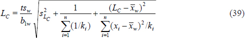
The previously described WLS prediction limit ![]() corresponds to the concept of a decision limit LC defined by Currie (1968) for the case in which the data arise from a calibration experiment, μ and σ at x = 0 are unknown, and one wishes to make a detection decision for a single future test sample. Measured concentrations (or instrument responses) that exceed the UPL should yield the binary decision of “detected” with (1 - α)100 percent confidence. Note that when the true concentation x = LC, the probability of exceeding the UPL is only 50 percent. As such, Currie defined the
corresponds to the concept of a decision limit LC defined by Currie (1968) for the case in which the data arise from a calibration experiment, μ and σ at x = 0 are unknown, and one wishes to make a detection decision for a single future test sample. Measured concentrations (or instrument responses) that exceed the UPL should yield the binary decision of “detected” with (1 - α)100 percent confidence. Note that when the true concentation x = LC, the probability of exceeding the UPL is only 50 percent. As such, Currie defined the
detection limit LD as the 95 percent UPL for a true concentration at LC. The WLS estimate of LC is therefore
and the WLS estimate of LD is
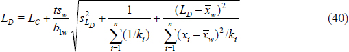
Note that in order to compute LC and LD, one must have estimates of ![]() and
and ![]() , which are often unavailable and must be estimated using a model of standard deviation versus concentration, as previously described. The final estimates of LC and LD are obtained from simple repeated substitution beginning from LC =0 and LD = LCuntil convergence (i.e., change of less than 10-4 in estimates of LC and LD on successive iterations).
, which are often unavailable and must be estimated using a model of standard deviation versus concentration, as previously described. The final estimates of LC and LD are obtained from simple repeated substitution beginning from LC =0 and LD = LCuntil convergence (i.e., change of less than 10-4 in estimates of LC and LD on successive iterations).
Finally, Currie (1968) defined the limit of determination LQ as the concentration at which the signal-to-noise ratio is 10 to 1. In the current context, one can estimate LQ by identifying the true concentration at which the estimated standard deviation is one-tenth of its magnitude. Again, a simple iterative approach generally performs quite well (Gibbons and Coleman, 2001; Gibbons et al., 1997).
REFERENCES
Bhaumik, D. and R. Gibbons. 2005. Confidence regions for random-effects calibration curves with heteroscedastic errors. Technometrics 47(2): 223-231.
Carroll, R. and D. Rupert. 1988. Transformation and Weighting in Regression. Boca Raton, FL: CRC Press.
Currie, L. 1968. Limits for qualitative detection and quantitative determination: Application to radiochemistry. Analytical Chemistry 40(3): 586-593.
Currie, L. 1995. Nomenclature in evaluation of analytical methods including detection and quantification capabilities. Pure and Applied Chemistry 67: 1699-1723.
Gibbons, R. 1995. Some statistical and conceptual issues in the detection of low-level environmental pollutants. Environmental and Ecological Statistics 2(2): 125-145.
Gibbons, R. and D. Bhaumik. 2001. Weighted random-effects regression models with applications to interlaboratory calibration. Technometrics 43(2): 192-198.
Gibbons, R. and D. Coleman. 2001. Statistical Methods for Detection and Quantification of Environmental Contamination. New York, N.Y.: John Wiley & Sons, Inc.
Gibbons, R., D. Coleman, and R. Maddalone. 1997. An alternate minimum level definition for analytical quantification. Environmental Science & Technology 31(7): 2071-2077.
Neter, J., W. Wasserman, and M. Kutner. 1990. Applied Linear Regression Models, 2nd Ed. Homewood, IL: McGraw-Hill/Irwin.
Rocke, D. and B. Durbin. 1998. Models and Estimators for Analytical Measurement Methods with Non-constant Variance. Davis, Calif.: University of California at Davis, Center for Image Processing and Integrated Computing.
Rocke, D. and S. Lorenzato. 1995. A two-component model for measurement error in analytical chemistry. Technometrics 37(2): 176-184.
Snedecor, G. and W. Cochran. 1989. Statistical Methods. Ames, IA: Iowa University Press.
This page is blank


