
5
Statistical Methods and Measurement
The central focus of the present committee’s activities is to evaluate the potential for new measurement technologies to make real-time and localized measurements for the presence of chemical agents at the Pueblo Chemical Agent Destruction Pilot Plant (PCAPP) and the Blue Grass Chemical Agent Destruction Pilot Plant (BGCAPP), including the possibility of making quick measurements on surfaces and detecting and quantifying low-level contamination.
New measurement capabilities might make possible more efficient and more reliable procedures. For example, using some of the new analytical technologies identified in Chapter 4, there are now quick and reliable means to detect and, if appropriate calibration standards are available, to quantify agent contamination on surfaces and hidden in crevices or other occluded places in machinery or building materials. Using these methods, it is now possible to more efficiently identify and delimit local hot spots of contamination, allowing a more efficient sorting of waste streams from the deconstruction process into segregated “contaminated” and “not contaminated” streams, each of which could get appropriate handling. The ability to conduct such segregation could enhance the speed of handling contaminated material and free the handling of uncontaminated material from onerous precautionary processes that may be unecessary in the absence of contamination.
To begin, some broad and overarching observations are worth noting. First, there are two broad categories of detection and measurement issues: (1) “monitoring,” which is used to check the adequacy of and detect inadvertent failures of current work practices, procedures, and protocols; and (2) “detection and characterization of contamination,” which aims at providing the basis for confident segregation and characterization of waste streams, identification of contaminated equipment, or parts of equipment, or areas of the facility that might have become contaminated with agent through routine operations or mishaps and malfunctions.
Overall, the following monitoring and measurement issues arise:
• Safety of workplace air for workers. Airborne agent monitoring is routine at chemical weapons demilitarization facilities, both to assure short-term air standards to protect against acute agent exposure effects and to establish that longer term standards designed to protect against any toxicity from ongoing
lower-level exposure have been met. The instruments and methods used for these purposes were reviewed in earlier National Research Council (NRC) reports (e.g., NRC, 2005a) and are not the subject of this report. Proactive evaluations of potential agent vapor sources that might lead to contaminated air (e.g., identifying potential agent vapor sources during maintenance or deconstruction activities) are a second element that may be aided by the new technologies discussed in Chapter 4.
• Contamination of local ambient air. During operations, the heating, ventilation, and air conditioning (HVAC) outflow is monitored with traditional methods for measuring airborne agents. During deconstruction, the containment and processing of the workplace air will no longer be in operation, and fugitive agent emissions from the site resulting from off- gassing from no-longer-contained contaminated materials may be an issue. Current airborne monitoring methods can detect any significant agent vapor concentrations. However, new surface analysis technologies may be useful in directing efficient decontamination activities, thus reducing the possibility of airborne agent contamination.
• Monitoring waste streams. During operations, agent monitoring can verify that procedures for preventing contamination are effective or assure that decontamination of any agent in or on protective gear and other waste streams are adequate. Waste streams of interest include used protective equipment, processed shell and rocket casings and other packaging materials, and the output of the chemical destruction process itself. Agent monitoring goals include assuring that workers handling waste streams are not subject to acute risks from contaminated material that has uncharacteristically and unintentionally entered the waste stream; assuring that any low-level contamination of the stream does not pose a hazard to workers from long- term, low-level exposure; assuring that any fugitive emissions during transport and disposal of wastes are not of concern; and evaluating the long-term safety of the ultimate disposal and storage methods. It may be important to characterize the mass of agent being exported with a waste stream, even at very low concentrations.
• Detecting and characterizing incidents of accidental contamination or failure of containment. The aim is to detect agent contamination before it can spread and be redistributed or cross-contaminate a wider area or commingled material. For such incidents, measuring the degree of contamination and delimiting its spread and extent will be key to efficient handling of contaminated material. Proactive investigation of the amount of spread and redistribution of local contamination from even well-performing routine operations may be wise. Materials that may absorb or trap ambient air agent vapors (such as electrical insulation) may be worth assessing.
• Providing the basis for segregating contaminated from noncontaminated materials into segregated waste streams. This issue occurs during process operations but may be more pressing during the facility deconstruction. As noted above, challenges include the possible presence of hidden or occluded contamination that might escape easy detection using vapor monitoring but may be exposed during demolition, collection, and transport of the materials in question. Issues may include the need to screen large amounts of material quickly enough to enable efficient processing into segregated streams on an ongoing, real-time basis and the challenge of efficiently scanning for localized hot spots, where lack of contamination of specific samples may not be sufficient to rule out contamination of the aggregate. Fast and effective detection of agent-contaminated surfaces may provide additional protection to demolition workers against acute releases of hidden reservoirs of material and identify structures that need special care in their demolition.
There are several potential advantages of the new analytical approaches. First, the ability to identify the source of contamination in a complex matrix of potential sources can lead to more efficient detection of residual contamination by agent trapped in occluded spaces. Second, the ability to simultaneously evaluate multiple potential contaminants may also be an advantage of the new measurement capabilities. Third, the ability to detect a source by following an airborne agent concentration gradient with a real-time measurement can lead to more rapid and efficent identification of an agent vapor source and decrease the extent of residual contamination. Fourth, waste streams such as spent activated carbon that are not amenable to analysis of headspace vapors can be interrogated in real time using these new methods.
However, in order to realize the potential benefits listed above, it must first be determined that these new methods have sufficient precision and accuracy to support the required, real-time, low-level-of-agent detection and quantitation in routine practice. What is the sensitivity and specificity of these new methods relative to existing procedures? To what extent can significant residual contamination be identified by these new methods that may not be detectable using existing methods such as headspace vapor analyses? How often can the rapid, in situ capabilities offered by the new methods be used to significantly reduce the time and effort required for necessary routine maintenance, upset response, agent changeover, or closure deconstruction procedures?
REVIEW OF EXISTING AGENT MEASUREMENT APPROACHES
In reviewing the Assembled Chemical Weapons Alternatives (ACWA) documents, there is little detailed description of the statistical methodologies guiding current agent monitoring and measurement methods. Most available material is presented in the ACWA document Chemical Agent Laboratory and Monitoring Quality Assurance Plan (LMQAP) (U.S. Army, 2011b). On page 7 of the plan, the authors state the objective:
Ensure that each operated and maintained monitoring system will indicate by alarm at least 95 percent (%) of the time in the presence of agent at or above the applicable airborne exposure limits (AEL) presented in Section 3.1. A confidence interval of 95% shall be established through the collection of quality data to characterize day-to-day reliability (precision) and validity (accuracy).
However, it is unclear to which statistic the confidence interval applies. In terms of measurement, calibration can be based on as few as three concentration points and is evaluated using a correlation coefficient that will not detect systematic bias. Certification of the method is based on the U.S. EPA method detection limit as described in USEPA 40 CFR Part 136, Appendix B, and involves computing the standard deviation of seven replicate samples spiked at the practical quantitation limit (PQL) and then multiplied by the constant 3.14, which is the 99th percentile of Student’s t-distribution with six degrees of freedom. The PQL is typically set at 5-10 times the method detection limit (MDL) and is often called the expected quantitation limit (EQL). This somewhat circular logic (i.e., spike at 5-10 times the analyst’s anticipated MDL and then compute the MDL) can yield a wide range of possible detection limits based solely on what a particular analyst expects the result (i.e., the MDL) to be. As will be shown graphically in a later section, the standard deviation is a function of spiking concentration, so the estimated MDL will be a function of the EQL, or, more simply, what the analyst expects it to be. Calibration-based approaches to estimating detection and quantitation limits remove the arbitrariness of this process and provide more statistically rigorous estimates of these unknown quantities. The following section and Appendix D provide a detailed review of calibration and related performance measures that represent a major improvement over common practice.
Chapter 11 of the ACWA LMQAP, “Statistical Analyses,” presents statistical approaches to be applied to quality control, calibration, and corrective action data. The discussion is limited and would benefit greatly from further statistical consultation. For example, when computing the statistical response rate at the alarm level, equation 11-10 in the LMQAP assumes that the true population mean and variance are known and the analyte concentration has a normal distribution. However, all that is available from the measurement process is an estimate of the population mean and variance (i.e., the sample mean and variance) from a finite and potentially small number of measurements, drawn from an unknown distribution that is likely to be right skewed and nonnormal. Ignoring the uncertainty in the sample mean and variance will produce incorrect probability estimates. Similar problems for the statistical response rate at the reportable limit (equation 11-12 in the LMQAP) are also present. A more complete discussion of comparing measurements to regulatory standards or alarm limits (e.g., airborne exposure limit (AEL)) is presented in a later section of this chapter and in Appendix E.
In this section, the committee considers analytical issues related to how surface (or other) measurement techniques might be qualified as effective for use, including issues of calibration, determination of false-positive and false-negative rates at specified
response levels, and the dynamic range of an instrument. The perspective is that the measurement techniques considered in Chapter 4 are designed to offer real-time, spatially resolved quantification of agent contamination. Furthermore, the main value of techniques such as desorption electrospray ionization (DESI), direct analysis in real time (DART), and related techniques may be follow-up evaluation of (relatively larger) areas that have been identified as contaminated through headspace monitoring methods or generator knowledge. For example, the distribution of contamination associated with visually identified quantities of spilled agents can be quickly evaluated.
The most rigorous approach to modeling measurement uncertainty and related detection and quantification limits involves analysis of the calibration function. In order to estimate the parameters of the calibration function and its related properties, a series of reference samples with known concentrations spanning the range of the hypothesized detection and quantification limits are analyzed. Variability is determined by examining the deviations of the actual response signals (or measured concentrations) from the fitted regression line of response signal on known concentration. In these designs, it is generally assumed that the deviations from the fitted regression line are Gaussian distributed; however this is not a requirement for corresponding statistical inference. Both ordinary least squares (OLS) and weighted least squares (WLS) approaches to estimating the calibration function and related uncertainty intervals are commonly used. The advantage of the WLS approach is that it can accommodate nonconstant variance across the range of the calibration function. In general, the magnitude of the variance increases with increasing concentration.
A useful model for the relationship between concentration and variability was originally proposed by Rocke and Lorenzato (1995). This R&L model postulates that there is a small region of constant variability near zero, which then increases linearly with increasing concentration. With a model for the calibration function (e.g., a linear model) and a model for the variance function (e.g., the R&L model), a prediction interval for the calibration function that provides 99 percent confidence for a future measured concentration within the calibration range can be derived. Such intervals provide an estimate of uncertainty in the measured concentration and can also be used to derive a confidence interval for true concentration given the measured concentration. Furthermore, using this statistical methodology, estimates of the detection and quantitation limits can be obtained. The detection limit describes the point at which the analytical method allows a binary decision on whether the analyte is present in the sample, and the quantitation limit describes the concentration at which the signal-to-noise ratio is 10:1 (i.e., a relative standard deviation of 10 percent). All of these statistical estimates document the capabilities of the analytical method and are essential in rigorous environmental monitoring programs. Details of the statistical methodology are presented in Appendixes D and E and are illustrated in the example below.
To demonstrate the benefit of the statistical data analysis using the calibration methodology described above, the committee analyzed data obtained by H. Dupont Durst and coworkers. These data were summarized in Nilles et al. (2009).1
The spectral area data (for agent and an isotopically labeled agent internal standard) were acquired with a time-of-flight mass spectrometer. Measurement samples were obtained by dipping a closed glass capillary tube into agent solutions (GA, GB, VX, and HD) and then inserting it into the DART ion source. Data at multiple concentrations in low (20 ppb), medium (200 ppb) and high (1 ppm) ranges were available for VX in deionized water and VX in 2-propanol, and GA, GB, and HD in methylene chloride. Each calibration generally included seven replicates at each of six different concentrations. For purpose of illustration, the committee selected the middle concentration range because the instrument responses are well differentiated across the concentrations in all matrices. VX in deionized water and VX in 2-propanol were also reasonably well differentiated at the lower concentration calibration, but GA, GB, and HD in methylene chloride were not. Quite similar results were obtained for VX in both low- and medium-concentration calibrations. The R&L model was used to characterize the variance function. This illustration focuses on VX in deionized water. All computations were performed using the Detect software (Discerning Systems, Vancouver, Canada). Figure 5-1 displays the estimated calibration function for VX in deionized water. Figure 5-2 displays the estimated relationship between variability and concentration. Figure 5-3 displays the relationship between the percent relative standard deviation and concentration.
This analysis reveals that the binary detection decision for VX in deionized water can be made at 2.7 ppb with 99 percent confidence, with a detection limit of 5.4 ppb. Quantification (i.e., the concentration at which the signal-to-noise ratio is 10:1) is possible at concentrations at or above 11.2 ppb. Applying the same methodology to the lower calibration range yielded critical level LC = 2.5 ppb, detection limit level LD = 4.9 ppb, and quantitation level Lq = 10.3 ppb, indicating that the estimated quantities are relatively robust to the selection of the calibration range.
For comparison purposes, the committee also examined the data for VX in 2- propanol. Here, it obtained LC = 6.7 ppb, LD = 13.4 ppb, and Lq = 28.0 ppb. These results suggest a substantial matrix effect, indicating that it is more difficult to detect and quantify VX in 2-propanol than in deionized water.
For GA, GB, and HD in methylene chloride, the committee obtained the following:
GA: Lc = 16.4 ppb, LD= 32.8 ppb, and LQ= 67.0 ppb.
GB: Lc = 22.6 ppb, LD = 45.0 ppb, and LQ = 92.8 ppb.
HD: Lc = 11.0 ppb, LD= 22.1 ppb, and LQ= 46.7 ppb.
![]()
1The committee used an extended dataset provided by H. Dupont Durst, Edgewood Chemical Biological Center, CMA.
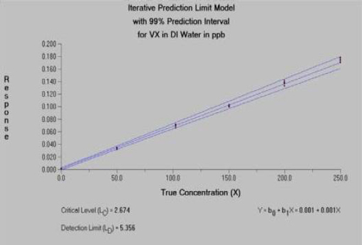
FIGURE 5-1 Estimated calibration function for VX in DI (deionized) water. SOURCE: Constructed from data provided by H. Dupont Durst, Edgewood Chemical Biological Center, CMA.
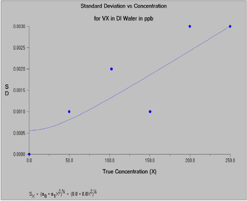
FIGURE 5-2 Estimated relationship between variability and concentration for VX in DI (deionized) water. SOURCE: Constructed from data provided by H. Dupont Durst, Edgewood Chemical Biological Center, CMA.
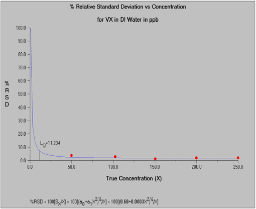
FIGURE 5-3 Relationship between the percent relative standard deviation (%RSD) and concentration for VX in DI (deionized) water. SOURCE: Constructed from data provided by H. Dupont Durst, Edgewood Chemical Biological Center, CMA.
It should be noted that the estimated detection and quantitation limits described here may not accurately represent expected performance for surface monitoring. Results obtained for single analytes in aqueous or liquid organic matrices may not be achievable in real- world applications. Additional challenges for chemical demilitarization surface data analyses include the presence of potential interferents; heterogeneous solid matrix properties; and heterogeneous analyte distributions and difficulty in introducing any internal standards. In the absence of internal calibration standards, the mean concentration for each physical sample (obtained from replicate samples) can be used as the reference and the methods described in Appendix D can then be applied.
Finding 5-1. New analytical methodologies (e.g., DART) have been demonstrated for relevant nerve agents (GB and VX) and blister agents (HD, HT, H) in simple liquid matrices (deionized water, isopropyl alcohol, and methylene chloride). Similar data for relevant surfaces (e.g., metal, concrete, activated carbon, plastics, and iron oxide) are sparse.
Recommendation 5-1. The use DART, DESI, or related new analytical methodologies for surface area measurements at the Pueblo Chemical Agent Destruction Pilot Plant or the Blue Grass Chemical Agent Destruction Pilot Plant requires that the quality of measurements be determined and related calibration studies be performed for relevant matrices.
Finding 5-2. Good precision and accuracy for DART techniques have been established for liquid matrices through the use of an internal standard. Challenges for development of internal standards for surface measurements include the presence of potential interferents; heterogeneous solid matrix properties; and heterogeneous analyte distributions and difficulty in introducing any internal standards. Development of internal standards for more homogeneous liquid and gas-phase matrices is more straightforward. The development of an internal standard may or may not be practical for some surface analysis applications at the Pueblo Chemical Agent Destruction Pilot Plant or the Blue Grass Chemical Agent Destruction Pilot Plant. In the absence of an internal standard, the precision of the quantitative measurements may decrease.
Recommendation 5-2. In the absence of an internal standard for surface measurements, the uncertainty in the measurement technologies (e.g., DART and DESI) should be established.
An important aspect of any monitoring program is demonstrating compliance with closure or remediation objectives. In the current context, the null hypothesis is that all surfaces, machinery, materials are contaminated and that the null hypothesis of contamination is rejected only when there is overwhelming evidence that the material in question is not contaminated. This specification of the null and alternative hypotheses leads to consideration on an upper bound on the true concentration of the analytes of interest, for example an upper confidence limit (UCL) for the mean concentration. To the extent that the UCL is beneath a health-based standard, cleanup objective, or worker safety threshold, it can be concluded that the material has been decontaminated, or that contamination was not present to begin with. This line of thinking can potentially lead to significant advantages in closure and related monitoring. If materials can be screened using new technologies, then headspace-type sampling and related analytical methods may not be required.
As an example, consider a surface such as a wall, which can be divided into grids. Wipe samples of each grid can then be used to produce a spatial distribution of analyte concentrations over the entire surface. If the spatial distribution is reasonably homogeneous (e.g., a nonsignificant random grid effect), then the average concentration of the grid measurements and the corresponding UCL can be estimated (based on an appropriate distribution for the chemical concentrations), and the UCL can be used to make a determination if further analytical or remedial work is required. Appendix E provides detailed parametric (normal, lognormal, gamma) and nonparametric methods for computing the appropriate UCL for relevant applications. If the spatial distribution is not homogeneous, then more local characterization of the concentration distribution can be performed and potential hot spots located and remediated until the distribution becomes homogeneous and an areawide determination can be made.
Finding 5-3. The published protocols for statistical procedures for compliance monitoring by the Assembled Chemical Weapons Alternatives program (i.e., in the draft Laboratory Monitoring Quality Assurance Plan, Rev. 0, April 4, 2011) contain insufficient detail to provide guidance for compliance monitoring. The ambiguity of current publicly available documentation suggests that quantification of statistical variability has the potential to be inaccurate. Such inaccuracies may result in difficulties such as unnecessary destruction of uncontaminated waste and/or failure to identify contaminated waste.
Recommendation 5-3. The Assembled Chemical Weapons Alternatives program should reexamine existing protocols planned for compliance monitoring at PCAPP and BGCAPP and means for incorporating increased statistical rigor in the assessments to be performed.
Measurement Bias, Precision, and Detection Limits
The “Analytical Measurements Issues” section in this chapter describes statistical approaches to understanding the information about a measurand (the quantity of interest) that can be inferred from one or more measurements. These discussions focus on measurement error as a source of random variability in measurement. With respect to the uncertainty associated with measurement error, calibration primarily refers to investigation of the relationship between a hypothetical “noiseless measurement” and the quantity being measured. In practice, calibration usually also refers to “correction” of a measurement system to eliminate measurement bias. In contrast, measurement precision refers to unreproducible random measurement error that leads to variation among multiple measurements of the same quantity.
In this section, it is assumed that the measurement systems of interest have been calibrated, so that bias has been eliminated. Conceptually then, a measurement can be thought of as the sum of the measurand and a random measurement error that has an expected (or long-run average) value of zero. The standard deviation of this random noise characterizes the precision of the measurement instrument (where a larger standard deviation corresponds to poorer precision). The precision associated with a measurement device can be improved by using the device to obtain multiple independent determinations of the same measurand and reporting the average of these as the measurement. In contrast, the bias associated with a measurement device cannot be reduced by repeated measurement; this fact underscores the critical importance of adequate calibration of any measurement system (Vardeman and Jobe, 1999).
Most measurement instruments used to determine the quantity or concentration of a substance also have a detection limit, a measurand value below which the instrument cannot discriminate true zero measurands from small positive values. When a measurement will be used alone (i.e., not along with other measurements in a more comprehensive analysis) and the detection limit is less than any applicable action level,
the detection limit has little or no practical implication. However, when the detection limit is not small relative to action levels, and/or multiple measurements are to be analyzed together, appropriate statistical treatment of the data can become more complicated. For example, simply substituting zero for the detection limit value for below-detection-limit readings can easily lead to seriously biased estimates and flawed conclusions. In these cases, appropriate censored data methods should be used to assure valid results (Helsel, 2004).2 However, while the more statistically rigorous analyses described above are more complicated than simple imputation methods, they may be captured in straightforward software routines to analyze ambient ionization data in real time and present evaluated data to the operator to guide further measurements.
Finding 5-4. Reliable real-time computer programs able to interpret real-time chemical analyses enable instruments (generally using proprietary software) to convert intensity measurements to concentrations of agents and potential interferents.
Recommendation 5-4. Instrument software for use with ambient ionization mass spectrometry should be reviewed to ensure that it meets appropriate validation and verification criteria. This software should be tested by using simulated data to test different measurement scenarios (e.g., all data below detection limits, at detection limits, mixtures, hot spots, and so on).
The measurement technologies used by ACWA, and those additional technologies that might also be considered, can be applied with different sampling strategies that correspond to substantially different definitions of “measurand.” In particular,
• Miniature continuous air monitoring system (MINICAMS) and depot area air monitoring system (DAAMS) measurements represent agent concentrations in air, integrated over fixed time intevals.
• DART and DESI techniques can be used to provide measurements of spatially resolved concentrations on surfaces.
Air concentration values have the most obvious connection to worker risk and so provide the basis for most existing standards and action values. However, where the challenge is to identify the location of quantities of adsorbed, absorbed, or trapped condensed-phase agent for decontamination, air concentration values are indirect and spatially indistinct indicators of the quantities of greatest interest. Conversely, while surface measurement techniques may accurately characterize the degree of contamination at a spatial point, such measurements are not efficient as a basis for screening a larger area or volume for contamination due to the number of such measurements that would be
![]()
2In statistical modeling, measurement data that may take on numerical values but may also result only in an indication that a threshold value has been exceeded (e.g., “below detection limits” or “above saturation level”) are termed “censored.” Statistical methods specifically designed to deal with such mixed data values are called “censored data methods.”
required. As discussed in the section “Hot Spot Detection” later in this chapter, the joint use of measurements representing different sampling modes may be an effective strategy in some settings.
In addition, surface measurements representing a larger basis than a near-point basis may also be achieved in some cases by some form of composite sampling—the collection and physical combination of material from several locations or over a continuous physical area—followed by one or more measurements of the combined sample. In particular, “wipe sampling” refers to a process in which a fabric matrix is passed across an extended area of the surface to be monitored and is then processed before a measurement is made. Such techniques can improve the efficiency of sampling activity, especially when the measurand is substantially below the action limit over most of the area to be characterized, because it may be possible to “clear” extensive areas using relatively few individual measurements.
However, when spatially integrated (e.g., composite) sampling is used, some thought must be given to how the resulting measurements should be related to the action levels. For example, if the intent of the standard is that no individual point on a surface have agent at a concentration above a specified level, wipe sampling may be only indirectly applicable if the concentration in the collected sample represents the average over the area wiped.3 In addition, there can be losses in efficiency associated with the process used to collect material; see, e.g., Verkouteren et al. (2008).
Finding 5-5. In some cases, analysis of direct surface and/or materials wipe sampling may complement or replace vapor screening level analysis, allowing more efficient and cost-effective closure operations.
Recommendation 5-5. If direct surface and/or materials wipe sampling analysis methods are adopted, appropriate statistical methods for characterizing the extent of contamination of surfaces, machinery, and/or materials should be employed.
In simple analytical applications where the measurement device is known to be well calibrated, it may be sufficient to limit analysis of measurement variation to random measurement error, considering only one measurand at a time. However, ACWA applications may also involve the use of one or more measurement methods within a spatial area4 to be monitored or characterized. For example, Scenario 3B (see Chapter 3) refers to demilitarization protective ensemble (DPE) suit entries into contaminated areas with the goal of identifying (the spatial location of) a source.
![]()
3In this sense, “average” refers to the mechanical process of collecting material over multiple locations or a contiguous surface. Single or repeated measurements of such combined samples may be expected to yield values that are between the extreme (high and low) concentrations that exist over the area sampled.
4A two- or three-dimensional region, such as a floor or room, over which agent concentration (on the surface or in the air) may vary. It is important to understand this variation, especially the more specific locations (in the spatial area) where concentration is unacceptably high.
In this context, a portable ambient ionization instrument, as described in Chapter 4, that produces a measurement of surface concentration of an agent specific to a location (actually, a small volume or area of surface, but here treated ideally as a point) within the region of interest may be used to collect data that can support the calculation of a contour map of concentration throughout that region. (For this discussion, the possibility that the measurand might change with time is ignored.) Regardless of the measurement technology used, it is clearly impossible to acquire a measurement at every spatial point of interest; at best, measurements taken at some collection of locations, or reflecting a “mechanically averaged” value over an area using a wipe, can be collected. As a result, there will be uncertainty stemming from spatial variability—the actual variation of the measurand across the area being studied—in addition to the uncertainty associated with measurement imprecision at any point. Specification of the nature of spatial variability is a critical step in deciding how samples should be collected, and how the resulting data should be analyzed for the purpose of monitoring or characterizing agent concentration in an area.
One widely used approach to spatial modeling describes the measurand as a stochastic spatial function of location within which concentration values are regarded as draws from a probability distribution (Cressie, 1993). Rather than being specified as independent draws at each location, they are modeled within a framework that allows statistical dependence, with stronger dependence for pairs of spatial locations that are separated by shorter distances.5 The result is that measurements collected at a fixed collection of spatial locations can be used to make useful predictions of concentration at other locations. One specific modeling method of this type, kriging,6 is widely used in environmental characterization studies and was employed first in mining applications where measurements at a collection of “core” sites were used to predict potential ore yield throughout an area or volume to be explored (Journel and Huijbregts, 1978).
Scenario 3B presents one possible setting for spatial modeling in the context of ACWA activities. If a spill has occurred in a work area and has been spread spatially by accidental contact or previous unsuccessful cleanup efforts, a spatially coherent (even if irregular) distribution of agent concentration may result. Sampling procedures that can efficiently acquire the measurements necessary to support reliable characterization of such agent deposits during DPE entries may be developed based on stochastic spatial models of agent concentration, so that areas requiring decontamination can be quickly identified.
Because the collection of measurements taken over a spatial domain is likely to be skewed in this context (i.e., many or most values are below detection, and perhaps a few are larger), the fidelity of spatial modeling may be improved by a nonlinear, monotonic transformation (such as a logarithm) of the measurand data No information is lost in
![]()
5In statistical modeling, two random quantities are “independent” if their values are completely unrelated, that is, if knowing the value of one does not influence what can be inferred about the other. “Dependent” random quantities, while each being subject to unpredictable noise, are related in such a way that knowing the value of one reduces the uncertainty in the other. For example, pairs of random quantities that are correlated (higher values of one are generally associated with either higher or lower values of the other) are dependent.
6Kriging is a statistical technique, originally developed for geological applications, that is used to estimate a continuous map of some quantity (e.g., a concentration) from measurements of that quantity taken at a discrete set of locations.
such a transformation, but the degree of spatial variability is typically more consistent in the transformed data, across the modeling domain. When modeling is done on a transformed scale, the resulting model (or “contour map”) can be reverse-transformed to the original, physically meaningful scale.
Sampling Plans for Spatial Modeling
There is no one optimal spatial sampling plan, even when a spatial variation model has been fully specified, because plans that are good for some purposes may be entirely inappropriate for others. For example, measurements may be collected within a defined spatial domain in order to support the following:
• Estimation of the parameters in a spatial model,
• Estimation or prediction of the measurand at a specified selection of locations not included in the sampling plan,
• Estimation or prediction of the integral or average of the measurand over the entire region of interest or a defined subregion,
• Estimation or prediction of the largest measurand within the region of interest, and
• Estimation or prediction of the location within the region of interest where the measurand is largest.
For any specified statistical model, each of these criteria may lead to different “optimal” sampling plans. However, within any specific application and for almost any realistic characterization goal, most reasonable sampling plans include:
• Measurements taken at a sufficient number of locations to provide reliable characterization of the spatial variation of the measurand across the region of interest and
• A sufficient number of replicate measurements at some locations to determine the magnitude of measurement errors being encountered or to validate the assumed precision of the instrument.
While the particular details of an efficient sampling plan must depend on specific goals and the details of the statistical model to be used, most reasonable models will lead to sampling plans with these two characteristics. Two general approaches to spatial sampling are briefly described below.
Fixed Sampling Plans
The simplest spatial sampling plans specify a collection of locations at which measurements are to be taken, and the number of replicate measurements to be taken at each location. For example, Scenario 3E anticipates that possible contamination over a
concrete surface may need to be characterized at facility closure in order to minimize the extent of scabbling. In this example, the floor of a 10 m x 10 m room might be sampled at 100 points, selected to cover the surface. These 100 points might be chosen randomly; however, randomly selected points often display clustering behavior. That is, some contiguous subregions may contain several selected sampling locations while others of similar size contain few or none. An approach that is often more reasonable is to use a distance-based measure to ensure that the 100 points selected cover the space as evenly as possible. Uniform discrepancy sampling designs (Fang et al., 2000) and maximin distance sampling designs (Johnson et al., 1990) are two approaches that can be more effective than simple random sampling of locations.
Generally, replicated measurements should be collected for at least some of the specified locations. In the committee’s hypothetical example, it might call for three replicate measurements to be made at each of the 100 locations in the room. Hence the overall sampling plan calls for 300 measurements in total. Given this restriction to 300 measurements, one might ask whether it would be more effective to collect four replicates at each of 75 locations (more replicate sampling at fewer spatial points) or two replicates at each of 150 locations (less replicate sampling at more spatial points). Determining an optimal balance requires some a priori generator knowledge of the relative sources of uncertainty associated with spatial variation of the measurand and with measurement error and also with the type of statistical model to be used for characterizing variability. In general, for measurement systems that are more noisy (i.e., that imply poorer measurement precision) relative to the actual variation in the measurand throughout the region, plans that sample at fewer distinct points and include more replicate measurements are preferred.
Sequential Sampling Plans
In contrast to fixed sampling, sequential sampling plans are designed so that later sampling locations are influenced by early measurements. Because one goal of sampling in this context is to identify subregions in which concentration is high, sequential sampling plans that use early measurements to get a rough idea of where these may be and carry out later measurements in the subregions that appear to be critical, can be more efficient than fixed sampling plans. The instruments described in Chapter 4 are rapid response (approximately 1 sec), making sequential sampling viable. As an alternative to the hypothetical fixed plan using 300 measurements described above, the following might be used.
A first stage of surface sampling might be carried out at 50 uniformly selected sites, with two replicate measurements at each point. Based on these 100 measurements and an acceptable statistical model, a “contour map” of agent concentration predictions of the measurand could be computed for the floor of the 10 m x 10 m room. This analysis will also yield standard errors, or confidence intervals, for the concentration at any point in the room. Some areas may be clearly below the applicable action value (i.e., with an upper confidence limit less than the action level), and some may be clearly above it (with a lower confidence limit greater than the action level). From a practical standpoint, there is little value in further sampling from either of these types of regions. Instead, a second
stage of sampling might be collected at 50 additional locations uniformly spread throughout the “ambiguous” regions, where upper and lower confidence limits of concentration are on either side of the action limit, perhaps again with two replicates at each location. A second analysis using all 200 data values collected in stages 1 and 2 will yield a more precise prediction of concentration in the areas that were initially difficult to classify, owing to the increased sampling intensity in these areas during the second phase of sampling. This process could then be extended to a third round of sampling, focused on regions that remain ambiguous based on the updated analysis.
Sequential sampling can be operationally impractical in applications where the analytical processing required for each measurement is substantial, or when the required data analysis between samples is complex. In contrast, sequential sampling appears to have great potential value when used with ambient ionization mass spectrometry because the latter provides location-specific data with very fast turn-around. Further, while interim formal statistical analysis may be needed in some cases, near-real-time results from these techniques will make it possible for workers to collect informal but informative sequences of measurements (without formal interim analysis) based on the characteristics of the sampled environment and the emerging patterns in the data.
Finding 5-6. The use of statistical sampling will improve agent contamination detection and quantitation. For near-real-time measurement technologies, sequential sampling may be particularly valuable. Specific sampling plans will depend on the geometry of the contaminated area, contaminant spatial variability, and the goal of the measurement process.
Recommendation 5-6. The Assembled Chemical Weapons Alternatives (ACWA) staff should have access to sufficient statistical expertise to develop effective sampling protocols for any application of ambient ionization monitoring. Once the resulting expert sampling protocols have been developed, ACWA headquarters monitoring staff or their contractors should then proceed to develop detailed standard operating procedures to guide monitoring technicians.
Another agent deposition pattern that may be especially relevant in the ACWA context could be formulated to describe one or a few hot spots in a region that otherwise has no agent or only a very low concentration of agent. Strictly speaking, this could also be regarded as a spatial pattern, but it is one in which there is relatively little spatial coherence and so relatively little opportunity to interpolate the measurand values at unsampled locations. Instead there are a few sparsely distributed but highly contaminated regions, and throughout the remainder of the area, contamination is comparatively low. For practical purposes, the important quantities to be determined are the elevated level and location of contamination.
In the context of Scenario 3D, it may not be sufficient to describe the occluded spaces using simple spatial coordinates. Cracks in concrete, pump chambers, and quantities of absorptive material may be pinpointed in space, but the specific
characteristics of these potential agent sinks and their patterns of operation may produce more helpful information than their physical coordinates. Here, potential hot spots coincide with these physically identifiable entities, and one or a few point-wise measurements within each may be a sufficient characterization.
The distinguishing characteristic of this model is the disconnected way in which it characterizes the contamination at each location, even within a spatial domain; essentially nothing is being assumed about spatial structure.7 That is, the model provides little or no basis for making any claim about what might exist at any unsampled locations. More specifically, there is no statistical basis for predicting or estimating the contamination at an unsampled location, no matter how close it is to the locations actually sampled. With sufficient sampling, including replicate measurements at some points, the model parameters (such as the mean and standard deviations representing measurement errors and the spatial variability of the contamination) may be estimable, and through this it may be possible to predict, for example, the proportion of the region of interest that exhibits significant contamination. But there may be little or no basis for identifying the sub-regions that may be most problematic.
From a modeling standpoint, hot spot phenomena are much more difficult to characterize than more gradually varying spatial patterns because of the noted lack of spatial coherency. Specifically, when hot spots comprise a relatively small area of volume compared to the region that must be screened, their location cannot be inferred by spatial interpolation from locations where the measurand is low. For practical purposes, a hot spot can be detected only by a measurement reflecting the concentration at the unknown location of the hot spot. For this purpose, sequential sampling plans that utilize multiple sampling bases may be most effective, as described below.
Sampling Plans for Hot Spot Detection
The fixed and sequential sampling plans described above can sometimes be useful in detecting isolated hot spots of agent concentration in spatial domains. However, if the hot spots are small in volume or area and the background concentrations do not “ramp up” to these elevated levels at nearby locations, the likelihood of identifying a hot spot with a spatially distributed collection of near-point measurements will often not be great.
Locating isolated agent deposits may be more effectively accomplished by a sequential strategy in which early samples are made on a broad area or air volume basis (e.g., headspace determinations), followed by measurements of wipe samples taken from limited surface areas, and finally with spatially resolved measurements.
The efficiency of sampling to identify hot spots may be improved substantially through the use of reliable generator knowledge in the temporal ordering of measurements. Ordered sampling suggests that there is some prior reason for making measurements at some locations earlier than at others. For example, in occluded space
![]()
7The kinds of spatial structure referred to might include continuity of the quantity of interest as a function of location, or any other characteristic that suggests a systematic connection between location and that quantity. In contrast, here the committee is discussing a model for which all pairs of spatial locations have the same relationship; for example, distance has no relationship to how much difference might be expected in the quantity of interest.
surveys (Scenario 3C), operation patterns and historical records will often suggest that some locations are more likely sources of agent than others. Arranging the order of measurements so that the elevated agent concentration is more likely to be found earlier rather than later can shorten inspection, at least in cases where a single reservoir can be tentatively assumed to be the source of contamination.
Finding 5-7. The successful application of any measurement technology is a function not only of its capabilities, but also of the ultimate use of the data generated. The context and purpose of the measurements will determine the sampling scheme, precision, and accuracy required.
A synopsis of the major issues identified in Chapters 1 through 5 is presented in the next and final chapter.


