
Appendix A
Population and Related Projections
Made by the Committee
Gretchen S. Donehower and Carl Boe
This appendix outlines the methods used to generate the population and labor force projections as well as summary measures and other indicators used in several chapters of this report. The projections were reviewed for accuracy and consistency by committee members and compared with results from other such projections. While the committee’s projections were made to 2100, the report primarily discusses results through 2050. Given the high degree of uncertainty regarding variables such as future rates of return, productivity growth, international capital flows, and so on, the committee chose to limit its analysis and discussion to the next four decades.
POPULATION PROJECTIONS BY AGE AND SEX
The population projections used by the committee are based on intermediate-cost population projections prepared by the Social Security Administration (SSA) for its 2011 Trustees Report, with some important modifications. The committee thanks Felicitie Bell, Office of the Chief Actuary of the SSA, for her generosity in sharing projection details with it. The Social Security methods are summarized here briefly, but complete information on SSA projection methods and assumptions can be found at http://www.ssa.gov/oact/tr/2011/index.html (accessed June 24, 2011). The starting population is the 2008 estimated Social Security Area population1
_____________
1The Social Security Area population covers the U.S. Census population (residents of all 50 states and Washington, D.C., plus Armed Forces overseas) but adds a small group of potential Social Security beneficiaries who are not covered by the U.S. Census population. These persons
by sex and single year of age. This population is projected forward each year based on projected rates of fertility, mortality, and net migration. Net migration is immigrants coming into the population minus emigrants leaving the population.
The age-specific fertility rates used are the same as in the intermediate-cost SSA projections, with a minor adjustment for the years 2008 and 2009.2 The age distribution of fertility is based on recent historical trends, while the overall level of fertility is assumed to decline gradually in the near term and remain constant at just below replacement level. Specifically, the observed total fertility rate is 2.09 children per woman in 2008 and is assumed to fall gradually to a constant level of 2.00 children per woman by 2035.
The main adjustment to the SSA projections is that the mortality rates used here are lower than those used in the intermediate-cost SSA projection. As described in Chapter 3, the committee agrees with the Social Security Advisory Board’s Technical Panel on Assumptions and Methods (TPAM) that there will likely be faster future declines in mortality than reflected in the intermediate-cost SSA projections. This conclusion is based on an analysis of potential future trends in smoking and obesity (Technical Panel on Assumptions and Methods, 2011). The SSA projection assumes that average life expectancy by 2050 will be 82.2 years, whereas the committee projection assumes instead an additional 2.3 years of life on average, for a life expectancy of 84.5 years by 2050. This mirrors the TPAM conclusion. The corresponding lower age-specific mortality rates are found by searching for a mortality schedule that is between the SSA intermediate- and high-cost options and implies a life expectancy in 2050 of 84.5 years. The high-cost option assumes lower mortality than the intermediate and thus an average life expectancy of 84.8 years by 2050. The projection used here employs a mortality schedule that is a weighted average of the two SSA options such that the desired life expectancy in 2050 of 84.5 years is achieved.
This average is found by first defining a difference term bx,s for age x and sex s, which is the difference between the death rates mx,s for the high cost and intermediate cost:
![]()
_____________
are U.S. citizens living abroad, residents of U.S. territories, and noncitizens living abroad who are insured for future Social Security benefits. They usually comprise around 2 percent of the U.S. Census population. In the aggregate, the Census and Social Security Area population age and sex distributions are almost identical.
2Published rates for 2008 were multiplied by 0.99 and for 2009 by 1.01 to match more closely the predicted birth cohorts of the SSA projections and correct for inconsistencies introduced by interpolation to estimate January 1 populations from July 1 population estimates.
The new death rates that were used for these projections are
![]()
where k, which is the same for both sexes and constant over age, is found by a search program to achieve the desired average life expectancy of 84.5 years in 2050.
The SSA projection adds net migrants at each projection step based on a guess about the future trend of migration, legal and illegal combined, and the age and sex distribution of net migrants from recent history. The total number of net migrants in the SSA projections begins at only 35,000 in 2008 based on evidence that the recent economic downturn in the United States has discouraged a great deal of potential immigration and encouraged some emigration. The projected number of net migrants quickly rebounds to 1,250,000 by 2015 but then falls slowly but steadily to 1,025,000 by 2085. While the committee’s projection uses the same age and sex distribution of net migration as in the SSA 2011 Trustees Report from 2008 to 2025, its trajectory for future migration is significantly higher than that of the SSA. As with future mortality, the committee believes that the future trajectory for net migration developed by the TPAM is more reasonable than the one currently used in intermediate SSA projections. Thus the committee adopted the TPAM migration schedule for 2026–2050, which assumes a constant rate of 3.2 net migrants for every 1,000 residents each year after 2025.
Given the rates of fertility, mortality, and net migration described above, the starting Social Security Area population of 2008 is projected forward in single-year steps of age and time for men and women separately using the cohort component method. The projection ends in the year 2100.3 This projection was the baseline scenario of future change. Summary measures for fertility, life expectancy, and net migration appear in Table A-1. For several analyses reported in previous chapters, the rates of fertility, mortality, and net migration were modified to calculate population projections based on alternative scenarios of change. In these cases, the projections were exactly as described above, except for the alternative rates described in the scenario.
_____________
3The SSA 2011 Trustees Report only published projection results to year 2085 because it is charged with reporting a 75-year time horizon for Social Security finances. The demographic projections, however, are estimated internally to 2100.
TABLE A-1 Summary Measures of Demographic Assumptions for Baseline Projection, Selected Years 2008–2100
| Years of Life Expectancy | |||||
| Year | Men | Women | Combined | Total Fertility Rate (births per woman) | Net Migrants (millions) |
| 2008 | 75.4 | 80.3 | 77.8 | 2.05 | 0.04 |
| 2009 | 75.6 | 80.4 | 77.9 | 2.04 | 0.84 |
| 2010 | 75.7 | 80.5 | 78.1 | 2.07 | 0.82 |
| 2015 | 76.9 | 81.3 | 79.0 | 2.05 | 1.25 |
| 2020 | 77.9 | 82.1 | 79.9 | 2.04 | 1.20 |
| 2025 | 78.8 | 82.9 | 80.8 | 2.02 | 1.14 |
| 2030 | 79.7 | 83.6 | 81.6 | 2.01 | 1.19 |
| 2035 | 80.5 | 84.3 | 82.4 | 2.00 | 1.23 |
| 2040 | 81.3 | 85.0 | 83.1 | 2.00 | 1.27 |
| 2045 | 82.1 | 85.7 | 83.8 | 2.00 | 1.31 |
| 2050 | 82.8 | 86.3 | 84.5 | 2.00 | 1.34 |
| 2055 | 83.5 | 86.9 | 85.1 | 2.00 | 1.38 |
| 2060 | 84.2 | 87.4 | 85.8 | 2.00 | 1.43 |
| 2065 | 84.8 | 88.0 | 86.3 | 2.00 | 1.47 |
| 2070 | 85.4 | 88.5 | 86.9 | 2.00 | 1.52 |
| 2075 | 86.0 | 89.0 | 87.4 | 2.00 | 1.57 |
| 2080 | 86.5 | 89.4 | 88.0 | 2.00 | 1.62 |
| 2085 | 87.1 | 89.9 | 88.5 | 2.00 | 1.67 |
| 2090 | 87.6 | 90.3 | 88.9 | 2.00 | 1.72 |
| 2095 | 88.1 | 90.7 | 89.4 | 2.00 | 1.78 |
| 2100 | 88.6 | 91.1 | 89.8 | 2.00 | 1.84 |
SOURCE: Committee calculations.
POPULATION PROJECTIONS BY RACE/ETHNIC GROUP
For some of the analyses, population projections by separate groups defined by race and ethnicity were of interest. The SSA does not take race or ethnicity into account when it makes projections, so data from the U.S. Census Bureau were used to break the SSA-based population projections into race/ethnic groups that are consistent with the main population projections used in this report. The committee thanks David Waddington, Ben Bolender, Christine Guarneri, and Donnette Willis of the Population Projections Branch of the U.S. Census Bureau for sharing data with it for the project.
Census Bureau projections are done based on the resident population by age, sex, race, and Hispanic origin. The set of projections published in 2008 was used here and can be found at http://www.census.gov/population/www/projections/2008projections.html (data first accessed May 31, 2011). These projections cover the years 2008 to 2050, so the committee extends the Census 2050 rates to the year 2100 to cover the full period of interest.
While the Census projections define many additional groups, only five groups were used in this work to avoid small numbers in groups defined by sex, single years of age, and race/ethnicity. The five race/ethnicity groups used were (1) Hispanic, (2) non-Hispanic white alone, (3) non-Hispanic black alone, (4) non-Hispanic Asian alone, and (5) non-Hispanic other. This last group includes non-Hispanic native Hawaiian and Pacific Islanders, American Indians and Alaska natives, and multiracial persons.
Census Bureau projected rates based on these five groups do not aggregate to the same rates as in the baseline single-group projection described in the preceding section. This is due both to the modifications in SSA rates made by the committee and to the different projection methods used by the Census Bureau and the SSA. To keep the projection by race/ethnic group consistent with the single-group projection, it was necessary to use the race/ethnic projections from Census to disaggregate the baseline projection rather than using Census rates by race/ethnic groups and projecting them directly.
This means that the starting population for the race/ethnic projections is not the starting population of the Census Bureau race/ethnic population projections. Instead, each age and sex group in the starting population for the single-group projection is broken down into the five race/ethnic groups based on the distribution in the Census Bureau population for that age and sex group.
Then, at each projection step, the total number of vital events (births, deaths, net migrants) for each age and sex group is estimated for the single-race projection and broken down into the five race/ethnic groups based on the distribution that would have occurred given the relative rates (of fertility, mortality, or net migration) from the Census Bureau race/ethnic population projections. In this way, the single-sex and race/ethnic projections are consistent with each other but the relative changes in the race/ethnic groups are consistent with the Census Bureau rates by race/ethnic group.
For example, say mortality rates for the single-group projection predicted 900 deaths to men aged 52 during the year, while the Census mortality rates by race/ethnic group projected 800 deaths across the five race/ ethnic groups. The 900 single-group deaths would be multiplied by the race/ ethnic distribution of the 800 deaths to get the race/ethnic distribution of the 900 deaths to men aged 52 during the year.
Finally, while the Census Bureau publishes mortality rates by each age/ sex/race/ethnic group, this is not the case for fertility or net migration. Birth rates are published by race/ethnic group only, not age, so the projection assumes that the age distribution of fertility for all five race/ethnic groups is the same as the overall SSA age distribution of fertility. Net migration is published as counts by sex and race/ethnic group, so the projection assumes that the age distribution of male net migration is the same as the SSA age
distribution of male net migrants for all five race/ethnic groups. Similarly for females, the SSA age distribution of female net migrants is used for all females across race/ethnic groups.
LABOR FORCE PROJECTIONS
The Bureau of Labor Statistics (BLS) usually projects the labor force only 10 years into the future. Occasionally, though, it extends those near-term projections to longer periods of time. The labor force projections in this report are based on labor force participation rates from a longer-term projection, one first produced in 2006 and later updated to a starting year of 2008. The method mainly takes historical trends within each age/sex/ race/ethnic group and extrapolates them into the future, but with a logit transformation so that the future path is nonlinear. During the first part of the projection period, through 2020, changes in the labor force “are the result not only of compositional changes in the population, but also of changes in the detailed labor force participation rates of the various age, sex, race, and ethnic categories. [These] latter changes are based on the past labor force behavior of those categories and are often assumed to approach zero beyond a certain point in the projection horizon. Accordingly, changes in the aggregate labor force participation rate and in the labor force between 2020 and 2050 will reflect only changes in the age, sex, race, and ethnic composition of the population.” (Toossi, 2006, p. 22) There is no economic model involved in the BLS projections, nor is there any attempt to include the effects of the business cycle.
The BLS data end in 2050, so the 2050 labor force participation rates were repeated to extend to a 2100 projection horizon. No estimates are provided for those younger than age 16, so their labor force participation rate is assumed to be zero. The details of the labor force projections can be found at http://www.bls.gov/opub/mlr/2006/11/art3full.pdf. (Data with projections through 2050 were accessed on July 11, 2011, but are no longer available on the BLS Web site.)
The BLS labor force participation rates are estimated by sex for single years of time, but for age the groups may span 2 years, 5 years, or more. To apply these rates to the population schedules by sex and single years of age, an interpolation method was used. A cubic spline was fitted to the cumulative counts of population and labor force, generating estimates of the total population and labor force at each age. The ratio of these produces labor force participation rates by single years of age that are completely consistent with the BLS age group rates but provide a smooth single-year-age schedule. These rates by sex and single year of age and time were then applied to the population projection described previously to get the total projected labor force by age and sex.
Note that the BLS labor force participation rates are based on a universe of the civilian noninstitutional population. They were applied here to a universe that includes noncivilians and the institutional population to avoid the need for estimating a further projection of future rates of military service and institutionalization by age, sex, and race/ethnic group. In the aggregate, the impact of the different population bases is very small.
The BLS does not include race/ethnicity in its labor force projections, so data from the March Current Population Survey (CPS) were used to estimate labor force participation rates by the same five race/ethnic groups discussed above. The CPS data were accessed through the Integrated Public Use Microdata Series facility, found at http://cps.ipums.org/cps/. Specifically, rates for the five groups from 2000 to 2011 were averaged together to estimate the labor force participation rates of the five groups within each age and sex group. Five-year age groups were initially estimated to reduce noise in the estimates, and then the same cumulative spline interpolation described above was applied to obtain a smooth single-year-of-age schedule. Then, a single multiplicative adjustment factor for each age-sex-year cell was computed so that the overall age-sex-year labor force participation rate was preserved; however, the race/ethnic groups had relative participation rates in the same ratios as the CPS rates by race/ethnicity for that age and sex.
SUPPORT RATIO ANALYSES
Calculating a support ratio requires two types of data: counts of population by age and per capita estimates of economic activity by age. The committee refers to the second item, the age schedules of per capita economic activity, as “age profiles.” The National Transfer Accounts project has a fully developed methodology for estimating age profiles of economic activity for individuals by age from surveys and administrative data. Details on the methodology are available at the project Web site, www.ntaccounts.org, and in Mason and Lee (2011). Examples of age profiles for consumption and production appear in Figure A-1 for the United States in 2007. Details on the sources and methods for constructing U.S. age profiles are found in Lee, Donehower, and Miller (2011).
A support ratio (SR) is the ratio of aggregate age profiles weighted by population. In mathematical notation, let c(x,t) and yl(x,t) represent the consumption and labor income profiles, respectively, in Figure A-1 at each age x at time t. Let n(x,t) be the number of persons age x in the population at time t. For a support ratio indicating the relative number of producers to consumers, the calculation is
![]()
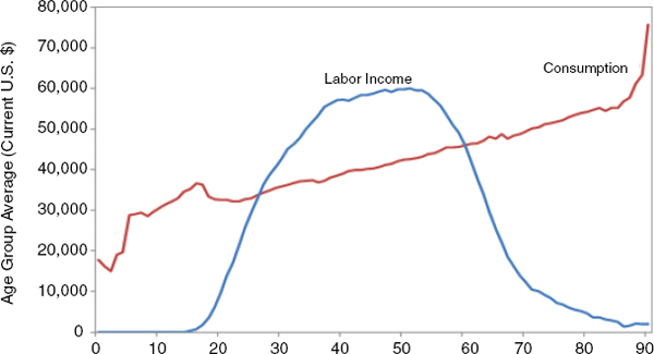
FIGURE A-1 U.S. per capita labor income and consumption, by single year of age, 2007. SOURCE: Committee calculations.
Similarly, a fiscal SR can be calculated substituting the age profile of taxes paid for labor income in the numerator and the age profile of government benefits received for consumption in the denominator.
The SR calculated for one time t in this way gives a snapshot of the aggregate balance between different pairs of age profiles at time t. If we combine the age profiles of a fixed time with a population projection, we can assess what will happen to the balance of age profiles, say labor income and consumption, over time if the age profiles remain fixed but the demography changes. For example, combining the age profiles shown in Figure A-1 with the U.S. population projection detailed in the first section allows generating a time series for t from 2007 to 2100:
![]()
This analysis was done for other countries with age profiles calculated as part of the National Transfer Accounts project, using the age profiles calculated for a recent year and combining them with population counts from the United Nations World Population Prospects database, medium variant projections (http://esa.un.org/wpp/unpp/panel_population.htm).
Calculating a time series of SRs in this way shows how population aging affects the ratio of producers to consumers or taxpayers to beneficiaries over time. It indicates what will happen if age profiles are held constant and population changes.
Another type of analysis asks how age profiles would have to change to maintain the level of the SR in the face of population aging. This was done by taking the labor income curve and extending the peak value for an additional year of age. For example, using 2007 age profiles for the United States and the population projection developed for this report, the support ratio in the United States for 2007 was 0.78. The peak value of average labor income was about $60,000 for people aged 51. Given population aging, the SR in the following year fell to just under that in 2007. Instead of allowing the support ratio to fall in 2008, the committee imagines that the age profile of labor income stretches at age 51, repeating the $60,000 value for age 52. The rest of the age profile shifts to the right by 1 year. The old age 52 value is assigned to age 53, and so on. Then the support ratio for 2008 becomes 0.80. This is above the initial 2007 value, so we proceed to the next year. The support ratio for 2009 to 2014 with the labor income curve stretched by 1 year is still above 0.78, so no further adjustment is needed. In 2015, however, the support ratio with the 1-year labor income extension falls below the 0.78 value, so the labor income curve must be extended again. Now labor income’s $60,000 peak value appears for ages 51, 52, and 53, and the original value for age 52 is assigned to age 54, for age 53 to age 55, and so on. Repeating this algorithm for the whole population projection gives an indication of roughly how many years retirement would have to be delayed on average to keep the SR from falling below its current level. This type of calculation can be made for other “thought experiments,” such as how much taxes would have to rise to maintain the current fiscal SR.
A different but more straightforward calculation indicates how much consumption would have to fall to maintain the current SR if labor income stayed fixed. That figure is simply the unadjusted SR divided by the SR in the starting year.
INCOME-WEIGHTED POPULATION
The future impacts of population aging may be conditioned by the socioeconomic conditions of countries with different future aging trajectories. To include this variable in the analysis, estimates of future population age distributions were calculated based not just on counts of population by age, but also by weighted population counts by age—that is, weighted by the relative wealth of the country where each projected person resides.
To review the basic population-weighted calculation where each person counts equally, let n(j,x,t) be the number of persons in country j of age x at time t. The global population age distribution, or the proportion of people in the world age q across all j countries at time t, is
![]()
which is the global number of persons aged q at time t divided by the global population at time t.
Now we can add a differential weight to each person in the calculation, based on the per capita gross domestic product (GDP) of each country j at time t, or GDP(j,t):
![]()
These analyses were done using several different data sources. The population by age and country were taken from the United Nations World Population Prospects database, medium variant projections for 2008, available at http://esa.un.org/wpp/unpp/panel_population.htm. Different GDP data were used to assess the robustness of the results to different data sources or scenarios.
One option was to use 2010 per capita GDP data for the entire projection period. The per capita GDP figures, measured in purchasing power parity-adjusted international dollars, came from the International Monetary Fund’s (IMF’s) World Economic Outlook database, the April 2011 version, available at http://www.imf.org/external/pubs/ft/weo/2011/01/weodata/download.aspx (accessed April 28, 2011).
Another option was to use per capita GDP figures for 2010 but multiply them by projected GDP growth rates to get a projected per capita GDP for each country. This was done using two different sources for the projected GDP growth rates. The first was the IMF World Economic Outlook database mentioned above, which has a projection of average annual growth from 2010 to 2016. This average annual rate was used to project each country’s GDP out to 2050, which was then divided by its projected population to get its projected per capita GDP (all adjusted for purchasing power parity). The second source was the consulting firm PriceWaterhouseCoopers, which estimates GDP growth using reports on future economic opportunities. Projected rates from 2010 to 2050 for 22 countries covering over 80 percent of 2010 global economic output are available at http://www.pwc.com/en_GX/gx/world-2050/pdf/world-in-2050-jan-2011.pdf (accessed April 28, 2011). As with the IMF projections, these rates were used to grow GDP from observed 2010 levels, which were then divided by projected population to get the per capita figures (also adjusted for purchasing power parity). For those countries not included in the PriceWaterhouseCoopers report, IMF data were used but adjusted by the ratio of the average PriceWaterhouseCoopers growth estimates to the IMF growth estimates for the 22 countries with data from both sources.
A few disputed territories or small islands that did not have both population and GDP projection data were dropped from the analysis.
TOTAL NET WORTH
If net worth differs by age, then population aging will have an impact on total net worth and thus the pool of assets available to an economy to fund growth. To examine this possibility, the committee used data on the average net worth of families in the United States by the age of the family head. These data come from the 2007 wave of the Survey of Consumer Finances (SCF), reported in the Federal Reserve’s February 2009 Bulletin (available at http://www.federalreserve.gov/pubs/bulletin/2009/pdf/scf09.pdf).
Let NW(x,t) be the average net worth of a family with head age x at time t. In order to apply this family measure to individuals, the committee assumed that all assets are owned by the head of the family and that nonheads have no assets. When NW(x,t) is multiplied by the headship rate h(x,t), or the proportion of persons age x who are family heads at time t, the product is the average net worth of a person age x at time t.4 The data on headship come from the 2007 March Supplement of the CPS. The CPS data were accessed through the Integrated Public Use Microdata Series facility found at http://cps.ipums.org/cps/.5
Finally, multiplying the average net worth per person in 2007, NW(x,2007)h(x,2007), by the population schedule n(x,t) gives the total net worth at time t. Dividing through by the total population gives the per capita amount:
![]()
As with the other calculations in this report, the committee is interested in the change brought about by population aging. This formula gives some indication of that by showing what will happen to per capita net worth in the future if the age profile of net worth and headship remain constant but the population continues to age.
_____________
4Note that NW(x,t) is the ratio of total net worth of families headed by those age x to the number of families headed by those age x. The headship rate h(x,t) is the ratio of the number of families headed by those age x to the number of persons age x. Multiply these two quantities together and the family terms cancel, leaving a ratio of total net worth of families headed by those age x to the number of persons age x. This is per capita net worth if we assume that only family heads own the assets.
5The concept of family in the CPS is not exactly the same as that in the SCF, so the headship data used from the CPS are the headship rates for households, not families. Across the entire population, the differences in family and household headship are small, as most households contain only one family, by both the SCF and CPS definitions.
STOCHASTIC POPULATION PROJECTIONS
Stochastic forecasts of fertility and mortality rates by age and sex, together with initial population counts and a deterministic migration schedule, allow for the generation of stochastic population trajectories through time that reflect uncertainty or variation around a long-term trend. The stochastic population counts (denoted Ns,x,ti, where the indices are sex (s), age (x), and time (t) and where i indicates a specific trajectory) in turn yield stochastic support ratios, SRit.
The level of uncertainty is a function of the amount of natural variation in the historical vital rates and in the forecast uncertainties of mortality and fertility components. The methodology is that described in Lee and Tuljapurkar (1994), where the Lee-Carter model is used for both the mortality and fertility components.
Mortality
Stochastic mortality trajectories were generated following the coherent forecast technique of Li and Lee (2005), which is a Lee-Carter model. This coherent method lowers forecast uncertainty by grouping forecasts for 15 low-mortality countries. Inputs to the model are mortality rates for 1950–2007 from the Human Mortality Database (University of California, Berkeley, and Max Planck Institute for Demographic Research, 2011); output consists of 1,000 stochastic sex-age-time trajectories Ms,x,ti from the online LCfit program (available at http://simsoc.demog.berkeley.edu/). Each projection i is independent from projection j ≠, i, and any life table functional such as e0 may be computed from the set of underlying death rates by fixing the trajectory number, time, and sex. The median in 2050 of the 1,000 trajectories for combined-sex e0 is close to 84.5, the target value from the baseline deterministic mortality projections in Table A-1.
The trajectories Ms,x,ti are “calibrated” so that the median of e0 for each sex matches up with the baseline values in Table A-1. Specifically, multipliers zs,t near unity are calculated so that
![]()
This affects the cloud of trajectories by changing the center while preserving the density of the cloud about the center.
Fertility
The fertility forecasts consist of simulations from a Lee-Carter model of age-specific fertility rates (ASFR), using data from the 2011 Trustees Re-
port of the Social Security Administration (http://www.ssa.gov/oact/tr/2011/index.html) and the small adjustments to data circa 2008 described earlier. The least-squares fit provided by the singular value decomposition of the 1917–2010 series of ASFR yields i trajectories:
![]()
where ax = ASFRx,2010i and Σ|bx| = 1 and Kti is a constrained autoregressive moving average (1,1) process with autoregressive coefficient 0.9673 and moving average coefficient 0.5367. The process is constrained so that the long-run average total fertility rate is 2.0 (see Lee and Tuljapurkar, 1994, for further details).
Migration
Net migration flows into the population follow the assumptions used in the deterministic population projections by age and sex (see Table A-1). Each stochastic trajectory experiences the same migration pattern.
Population
A population trajectory i begins with the initial launch population by age and sex in 2009, Ns,x,2009i. To bring this population to 2010, losses from death during the year and additions from new births are determined using rates Ms,x,2009i and ASFRs,x,2009i applied to the population. Finally, immigrants are added according to the baseline schedule.
Support Ratio
The SR for the i th trajectory,
![]()
is calculated along the trajectory based on the stochastic population counts. The consumption schedule c(x,t) is normalized so that the support ratio in 2007 is unity.


