
Around the world populations are aging. This is a relatively new demographic phenomenon because for most of human history populations were young and lives were short. Population aging is largely caused by two demographic trends. Most obviously, people today are living longer than before. A second and less obvious cause of population aging is a decline in the birth rate. With lower birth rates, younger generations are smaller relative to older generations, thus raising the average age of the population. There are other demographic processes that affect aging, including migration, but they generally play a smaller role.
This chapter will examine these trends in the United States, starting with improvements in life expectancy and their implications for the individual life cycle. Later sections of the chapter will discuss population aging and why it matters.
LIFE EXPECTANCY AND THE INDIVIDUAL LIFE CYCLE
Life Expectancy at Birth
U.S. life expectancy at birth started improving in the eighteenth century, reaching 47.3 years in 1900, 68.4 years in 1950, and 78.2 in 2010 (Arias, 2011; Board of Trustees, Federal Old-Age and Survivors Insurance and Federal Disability Insurance Trust Funds, 2011). Increases were most rapid in the first half of the twentieth century, when infectious diseases were brought under control, greatly improving survival of children. In contrast, increases in life expectancy since 1950 have been due mostly to declines in adult mor-
tality as cardiovascular disease became more manageable. The rise of 9.3 years in the United States between 1950 and 2006 was substantial, but most other countries in the world achieved more rapid improvements over the same period. Figure 3-1 compares trends in life expectancy for the United States (black line) and eight other large high-income countries (Australia,
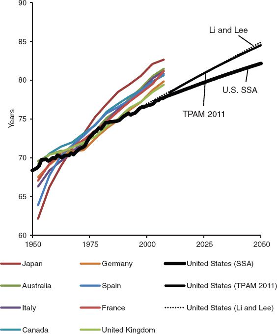
FIGURE 3-1 Life expectancy at birth in selected countries, and alternative projections for the United States to 2050. SOURCES: United Nations (2011); Board of Trustees, Federal Old-Age and Survivors Insurance and Federal Disability Insurance Trust Funds (2011); Li and Lee (2005); and Technical Panel on Assumptions and Methods (2011).
Canada, France, Germany, Italy, Japan, Spain, and the United Kingdom). The United States ranked at the top of this group of countries in 1950 but dropped to last place in 2006 (United Nations, 2011).
Why does the United States now rank so low in international life expectancy comparisons? This question has drawn the attention and concern of researchers and policy makers. The current situation is especially surprising given that the United States spends far more on health care than any other country. In response to these concerns, the National Research Council (NRC) appointed a committee of experts in 2008 to investigate the reasons for this divergence between the United States and other high-income countries. In its final report the committee reached several conclusions (National Research Council, 2011):
A history of heavy smoking and current levels of obesity are playing a substantial role in the relatively poor longevity performance of the United States. (p. S-4)
The damage caused by smoking was estimated to account for 78 percent of the gap in life expectancy for women and 41 percent of the gap for men between the United States and other high income countries in 2003. (p. S-2)
Obesity may account for a fifth to a third of the shortfall of life expectancy in the United States relative to the other countries studied. (p. S-2)
What are the implications of these conclusions for future trends in life expectancy? Mortality will likely continue to decline as further progress is made in medicine, biotechnology, public health, nutrition, access to medical services, incomes, and education. However, substantial disagreement exists among analysts about how rapidly future improvements will occur (Bongaarts, 2006; Wilmoth, 1997 and 2001). At one end of the spectrum of opinion are pessimists (Carnes, Olshansky, and Grahn, 1996; Olshansky et al., 2005), who believe that the most advanced countries are close to a biological limit to longevity. A very different opinion is held by optimists (Oeppen and Vaupel, 2002), who expect life expectancy at birth to continue to rise very rapidly, reaching over 100 years later this century. Most projections by researchers and government agencies fall between these extremes (Lee and Carter, 1992; Li and Lee, 2005; Tuljapurkar, Li, and Boe, 2000; Bongaarts, 2006). The best-known U.S. projection is the one used by the Social Security Administration. The 2011 Report of the Board of Trustees of the Federal Old-Age and Survivors Insurance and Federal Disability Insurance Trust Funds (commonly known as the Trustees Report) projects life expectancy to reach 82.2 years in 2050, up from 77.7 in 2006.
In 2010 the Social Security Advisory Board appointed the Technical Panel on Assumptions and Methods (TPAM) to assess the assumptions and methods used in the Trustees Report. The TPAM made a number of
recommendations, including a significant revision of mortality projections. The conclusion that increases in life expectancy will likely be more rapid than is currently assumed in the Trustees Report is based on an analysis of potential future trends in smoking and obesity (Technical Panel on Assumptions and Methods, 2011). The TPAM noted that the slow pace of improvement in life expectancy over recent decades was due to the impact of smoking and obesity and that these behavioral effects will likely continue to depress U.S. life expectancy. However, after rising for decades, indicators for smoking and obesity have now plateaued. According to the 2011 NRC report mentioned above:
After 1964, when the Surgeon General’s Office released its authoritative report on the adverse effects of cigarette smoking, the increase in smoking slowed, stopped and eventually reversed in the United States. (p. 5–4)
Recent data on obesity for the United States suggest that its prevalence has leveled off and some studies indicate that the mortality risk associated with obesity has declined. (p. S-4)
The TPAM therefore assumed that the adverse impact of these behaviors on life expectancy will remain at, or close to, current levels rather than rise much further in the future. Taking these trends into account, the TPAM expects U.S. life expectancy to reach 84.5 years in 2050. This estimate is close to a widely used and respected projection made by Li and Lee (2005) but above the 2011 Trustees Report assumption of 82.2 years. As shown in Figure 3-1, the future pace of improvement is more rapid than assumed in the Trustees Report but still slightly slower than the pace achieved by other high-income countries in past decades.
The projections of life expectancy, population aging, and other demographic indicators used in the present report are based on special projections made by the committee to incorporate the higher trend in life expectancy recommended by the Social Security TPAM (see Appendix A).
Life Expectancy at Older Ages
Remaining male life expectancy for those aged 65 in 2010 equaled 17.5 years, but it dropped to 10.8 years for those aged 75 and to 5.7 years at age 85 (Table 3-1). At all ages women have more years remaining than men. The committee’s projections indicate an ongoing upward trend in remaining life expectancy at these older ages as well, with life expectancy at 65 reaching 22.2 years for males and 24.1 years for females in 2050. It is noteworthy that Japanese females had already achieved in 2009 the life expectancy that U.S. women are not projected to reach until 2050 (Organisation for Economic Co-operation and Development, 2011). The declines in remain-
TABLE 3-1 Years of Remaining Life at Older Ages in the United States: 1950, 2010, and 2050
| Age | Gender | 1950 | 2010 | 2050 |
| 65 | Male | 12.8 | 17.5 | 22.2 |
| Female | 15.1 | 19.9 | 24.1 | |
| 75 | Male | 7.9 | 10.8 | 14.2 |
| Female | 9.0 | 12.5 | 15.6 | |
| 85 | Male | 4.5 | 5.7 | 7.6 |
| Female | 5.0 | 6.7 | 8.5 | |
SOURCES: 1950 and 2010 from Board of Trustees, Federal Old-Age and Survivors Insurance and Federal Disability Insurance Trust Funds (2011); 2050 from special projections prepared by the committee (see Appendix A).
ing life expectancy as people age are important for the later discussion of public support systems such as Social Security and Medicare.
Longer Life and the Individual Life Cycle
As discussed later in this chapter, population aging results in part from longer life and in part from lower fertility. Figure 3-2 plots the average number of years spent in the three main life cycle phases: (1) total not working (during childhood or adult years prior to age 60); (2) working (defined as being in the labor force); and (3) retired (over age 60 and not in the labor force). The sum of the years spent in these three phases equals the life expectancy at birth, as plotted in Figure 3-1.1
As longevity rises over time, people spend more time in retirement. Between 1962 and 2010 the average time spent in retirement rose by 5 years (from 10 to 15 years), while life expectancy rose by 8 years. During this period, years in the labor force increased modestly but years not working declined slightly. These trends are largely attributable to the increasing labor force participation of women (see Chapter 5). In 1950, only 10.6 years were spent retired, but by 2050 the years in retirement are projected to reach 20, nearly doubling, while working years rise from 31 to 40 and nonworking years remain nearly constant.
The U.S. population is devoting increasing years to retirement both in absolute terms and as a proportion of life. As shown in Figure 3-3, the proportion of life spent in retirement rose from 15 to 19 percent between 1962 and 2010 and is expected to reach 24 percent in 2050. The ratio of retired
_______________
1Estimates are based on labor force participation rates by age through 2010 provided by the Office of Critical Trends Analysis of the Social Security Administration. Labor force participation rates are held constant from 2010 to 2050.
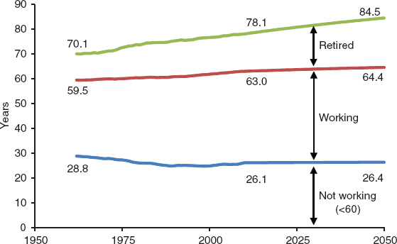
FIGURE 3-2 Years lived retired, working, and not working, 1962–2050. SOURCES: Board of Trustees, Federal Old-Age and Survivors Insurance and Federal Disability Insurance Trust Funds (2011) and projections by the committee.
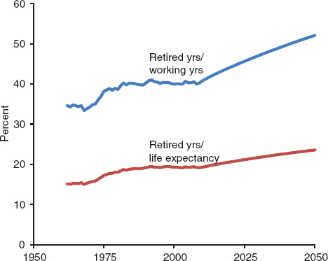
FIGURE 3-3 Retired years as a proportion of working years and of life expectancy, 1962–2050. SOURCES: Board of Trustees, Federal Old-Age and Survivors Insurance and Federal Disability Insurance Trust Funds (2011); and projections by the committee.
to working years also grew from 35 to 41 percent between 1962 and 2010. By 2050 this proportion is projected to be 52 percent, which implies that the average individual would then work 2 years for every year in retirement.
Adjusting the Life Cycle
As discussed in later chapters of this report, the costs of public support for health and pension benefits to the elderly will be difficult to bear given the rapid pace of population aging. Among the adaptations that are being considered is an increase in the age at retirement with full benefits, because the costs of this public support decline as the age of eligibility rises. It is useful to consider two simple demographic calculations to put this adaptation in context. In the first, we ask until what age a person would have to work in 2050 in order to have the same number of years in retirement as someone who retired at age 65 in 2010. The answer is 70.2 years.
Another useful calculation would be how many more years of work will be needed in the future to keep the ratio of retired years to working years constant at the 2010 level.2 As shown in Figure 3-4, a retirement age of just 60 years would have yielded the same ratio in 1950 as in 2010. Based on the committee’s projections, a rise of 4 years (from 65 to 69) would hold this ratio unchanged between 2010 and 2050. This scenario involves a smaller rise in the age at retirement and would allow some increase in years spent in retirement.
Socioeconomic and Geographic Variations in U.S. Life Expectancy
The preceding discussion focused on the average life expectancy in the United States and other countries. In addition to between-country variation in life expectancy there is substantial within-country variation, e.g., among racial and ethnic groups, among states and counties, and among groups with different levels of education and income.
Table 3-2 presents life expectancy for whites and blacks in 2008. White life expectancy at birth exceeds black life expectancy by 5 years (75.9 vs. 70.9) among males and by 3.4 years (80.8 vs. 77.4) among females. By age 65, these racial differences have declined to 1.8 years for males and 1.0 year for females. Analyses of ethnic differences usually find mortality among Hispanics to be lower than among whites. This so-called “Hispanic paradox” is probably due to a selection for good health among immigrants from Latin America and a tendency of Hispanic immigrants to return to their
_______________
2For this simulation, working years are calculated as years lived between age 20 and retirement age in a stationary population with current life expectancy. Retired years equal years of life remaining after retirement. Age at retirement is set at 65 in 2010.
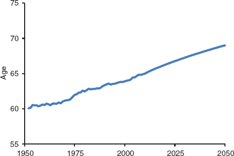
FIGURE 3-4 Hypothetical retirement age required to keep the 2010 ratio of retired to working years constant through 2050. SOURCES: Board of Trustees, Federal Old-Age and Survivors Insurance and Federal Disability Insurance Trust Funds (2011) and projections by the committee.
country of origin when they become ill (Elo and Preston, 1997; Markides and Eschbach, 2011).
Large mortality differences due to education level are found in the United States as well as in other countries. As shown in Table 3-3, life expectancy at age 25 in 1998 was 7.6 years less for males with less than 9 years of schooling compared to males with 13 or more years of schooling. Among females the difference between these two groups was 4.9 years. At age 65 these differences narrowed but remained a substantial 3.4 years for males and 2.5 years for females. A more recent analysis of trends through 2008 found that adults with fewer than 12 years of education in 2008 had life expectancies similar to the U.S. average in the 1950s and 1960s
TABLE 3-2 Years of Life Expectancy at Birth and at Age 65 for Whites and Blacks, 2008
| White | Black | Difference (White - Black) | |
| At birth | 78.4 | 74.3 | 4.1 |
| Male | 75.9 | 70.9 | 5.0 |
| Female | 80.8 | 77.4 | 3.4 |
| At age 65 | 18.7 | 17.5 | 1.2 |
| Male | 17.3 | 15.5 | 1.8 |
| Female | 19.9 | 18.9 | 1.0 |
SOURCE: U.S. Census Bureau (2012).
TABLE 3-3 Years of Life Expectancy at Ages 25 and 65 by Educational Attainment, 1998
| Years of Schooling | ||||
| 0–8 | 9–12 | 13+ | Difference (13+) - (0–8) | |
| At age 25 | ||||
| Male | 47.0 | 47.5 | 54.6 | 7.6 |
| Female | 52.9 | 53.6 | 57.8 | 4.9 |
| At age 65 | ||||
| Male | 14.9 | 15.1 | 18.3 | 3.4 |
| Female | 17.9 | 18.3 | 20.4 | 2.5 |
SOURCES: Data from Hummer and Lariscy (2011); Molla, Madans, and Wagener (2004).
(Olshansky et al., 2012). By combining education and race, the study showed large and growing differences in life expectancy between whites with 16+ years of schooling compared to blacks with fewer than 12 years of education.
Geographic differences in mortality are also well established. Life expectancy in 1999–2001 was highest in Hawaii and Minnesota and lowest in the District of Columbia and Mississippi (Table 3-4). Differences at the county level are even larger than among states (Ezzati et al., 2008).
The literature has proposed a range of factors that may be responsible for or contribute to these mortality differences. Generally, disadvantaged groups or populations smoke more, are more obese, exercise less, live more stressful lives; have less access to health care services; have fewer social resources and lower status occupations; live in neighborhoods with poor housing, high levels of pollution, and relatively high crime rates; and have less income and education (Centers for Disease Control and Prevention, 2011; National Research Council, 2004a, 2004b). Differences in genetic endowment may also play a role (Christensen and Vaupel, 2011). Despite the often significant correlation between these explanatory factors and mortality, it is difficult to disentangle the complex causal pathways and quantify the true determinants of mortality differences.
TABLE 3-4 Years of Life Expectancy at Birth and at Age 50 for Selected States/Areas, 1991–2001
| District of Columbia | Mississippi | ..… | Minnesota | Hawaii | Difference (Hawaii - D.C.) | |
| At birth | 72.3 | 73.6 | 79.0 | 79.7 | 7.4 | |
| At age 50 | 28.0 | 31.4 | 31.4 | 32.4 | 4.4 | |
SOURCE: Wilmoth, Boe, and Barbieri (2010).
These mortality differences have potentially important implications for the design of policies to address the adverse consequences of aging. In particular, raising the full retirement age for all retirees leads to a larger proportional reduction in expected years of retired life for disadvantaged groups than for advantaged groups. The committee believes that such a differential impact would be undesirable.
POPULATION AGING
Population Age Distribution
The older population in the United States is on the threshold of a boom. The population aged 65 and over will increase substantially between 2010 and 2030, reaching 72 million in 2030, more than twice the level (35 million) in the year 2000 (He et al., 2005; Vincent and Velkoff, 2010). Figure 3-5 shows broad changes in the nation’s age distribution from 1950 to 2010 and projected changes through 2050. This graphic highlights the growing share of people in older age groups and the corresponding decline in the share of the population under age 30. As discussed in more depth later in this chapter, the United States is aging less rapidly than most other high-income countries and may be relatively better able to cope with the pressures of demographic change.
Another view of changing age distribution is provided by Figure 3-6, which plots U.S. population size by age for 1975 and 2000 and as projected to 2025 and 2050. In 1975 a large proportion of the population was between 10 and 30 years of age. This group is often referred to as the baby boom generation, because it consists of the survivors of the large number of U.S. births between 1945 and 1965. As this generation ages, its presence in the age structure leaves a visible bulge that reaches ages 35–55 in 2000, ages 60–80 in 2025, and ages 85+ in 2050. The population aged 90+ rises more than 17-fold between 1975 and 2050. Over past decades, the baby boom postponed population aging as it moved through the labor force ages. But now it is ushering in a new period of very rapid population aging as it moves into old age.
The baby boom generation retires during the first quarter of the twenty-first century, causing a steep increase in the number of recipients of Social Security and Medicare benefits (Figure 3-7). The number of people reaching age 65 each year rose modestly between 1950 and 1980 and then fell for several years as a result of low birth rates during the Depression years of the 1930s. But between 2000 and 2025 the annual number of those turning age 65 is expected to more than double, from 2.1 to 4.3 million (the modest reduction after 2025 is due to the end of the baby boom in the 1960s).
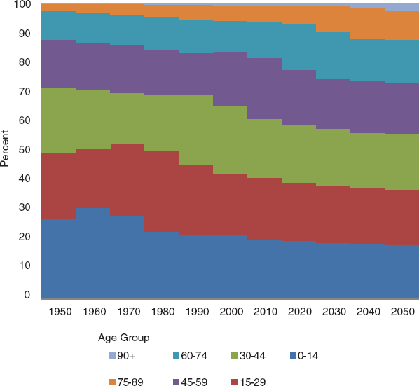
FIGURE 3-5 Percent distribution of the population by age, 1950–2050. SOURCES: Board of Trustees, Federal Old-Age and Survivors Insurance and Federal Disability Insurance Trust Funds (2011) and projections by the committee.
Providing pensions and health care for this wave of new retirees will be a challenge.
Demographic Drivers of Aging
The amount of aging the U.S. population will experience in the future depends on trends in mortality, fertility, and migration. In general, the lower the levels of fertility, mortality, and migration, the older the population will become. It should be stressed that if infant and younger-adult mortality rates remain relatively low for a prolonged time, as has been the case in most developed countries for many decades, changes in life expectancy at older ages become inceasingly important to changes in overall life expectancy. The demographic assumptions on fertility, mortality, and migration underlying the population projections in this report are discussed next.
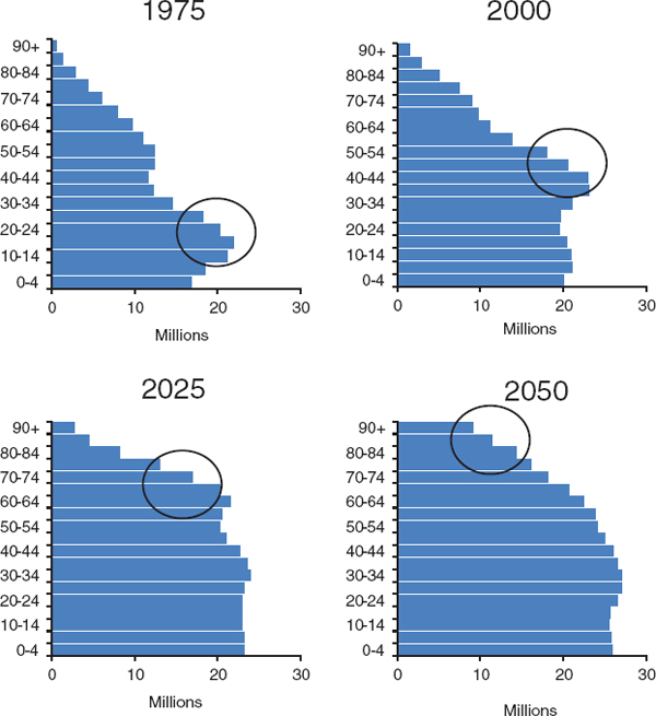
FIGURE 3-6 Population by age, 1975–2050. The circled groups approximate the baby boom as it moves through time. SOURCES: Board of Trustees, Federal Old-Age and Survivors Insurance and Federal Disability Insurance Trust Funds (2011) and projections by the committee.
Fertility
Past estimates and projections of fertility as measured by the total fertility rate (TFR) are plotted in Figure 3-8. Over the past half-century the TFR has fluctuated widely in response to a range of social and economic developments. Fertility rose sharply after the Second World War, reaching 3.7 births per woman at the peak of the baby boom in 1957. The next two
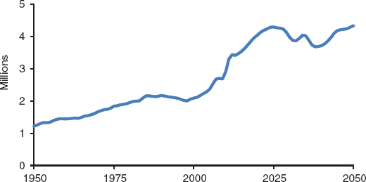
FIGURE 3-7 Number of people turning 65, 1950–2050. SOURCES: Board of Trustees, Federal Old-Age and Survivors Insurance and Federal Disability Insurance Trust Funds (2011) and projections by the committee.
decades saw a steep decline to 1.7 births per woman in 1976. Over the next three decades, the TFR slowly recovered, reaching an average just below 2.1 during the period 2006–2010.3 The 2011 Trustees Report assumes a small decline to 2.0 will occur over the next two decades. This assumption was reviewed by the 2011 TPAM and found to be reasonable, and it is incorporated into the population projections used in this report.
Mortality
As noted earlier, the Social Security Advisory Board’s TPAM has recommended assuming a U.S. life expectancy of 84.5 years in 2050, and this assumption has been adopted in the population projections used in the present report.
Migration
Net migration, legal and illegal, rose from 0.8 to 1.9 million per year between 1980 and 2005 (see Figure 3-9, solid line). The recession of the late 2000s reduced this number to near zero in 2008, followed by a rebound in 2009 and 2010. These large recent swings are mostly due to changes in illegal migration, which is estimated to have turned negative in 2007. Legal
_______________
3The total fertility rate was between 2.0 and 2.1 births per woman during the period 2000–2005 and reached 2.1 in 2006 and 2007. The TFR declined modestly after 2007 in conjunction with the economic downturn, to a level between 1.9 and 2.0 according to preliminary 2010 data (National Center for Health Statistics, 2011).
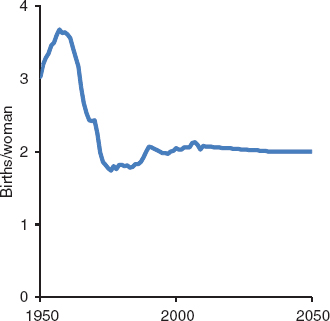
FIGURE 3-8 Total fertility rate, 1950–2050. SOURCE: Board of Trustees, Federal Old-Age and Survivors Insurance and Federal Disability Insurance Trust Funds (2011).
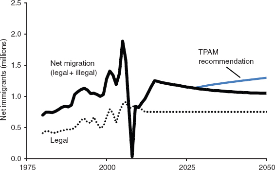
FIGURE 3-9 Net migration, 1980–2050. SOURCES: Board of Trustees, Federal Old-Age and Survivors Insurance and Federal Disability Insurance Trust Funds (2011) and Technical Panel on Assumptions and Methods (2011).
net migration shows only minor fluctuations. The fairly steady past rise in legal migration comes from the implementation of new legislation allowing a larger influx in recent decades.
The Social Security Trustees Report projects that the rebound in migration will continue until 2015 before beginning a steady decline over future decades. This decline is assumed to be entirely in illegal migration; legal migration is held constant at 750,000 from 2012 onward following current law. The TPAM reviewed these projections and accepted the projections from 2010 to 2025 but recommended an increase in the projected flow of migrants after 2025. There are two main reasons for this recommendation: (1) the population of the United States and the sending countries is expected to grow in future decades and (2) current law will probably change to allow more legal migration. The projections in the present report incorporate this higher migration trajectory recommended by the TPAM.
Because migrants are on average younger than the U.S. population, migration reduces population aging. The impact of migration can be es-
BOX 3-1
The Impact of Demographic Alternatives
Since trends in fertility, migration, and mortality are the direct determinants of trends in the population age structure, it is reasonable to consider policies that could reduce future population aging by changing these determinants. Raising mortality is, of course, not a realistic option, but fertility and migration could be changed through government intervention.
To illustrate the likely effects of demographic alternatives, the committee poses the question, How would levels of fertility and migration have to change (relative to the committee’s preferred assumptions—see Appendix A) to achieve a 10 percent reduction in the old age dependency ratio (OADR) by the year 2050? In other words, what amount of change would reduce the expected 2050 OADR of about 0.39 shown in Figure 3-13 to 0.35?
Current projections made by the Social Security Trustees and accepted by the committee assume that the U.S. total fertility rate will decline very modestly from about 2.1 births per woman during the period 2006–2010 to 2.0 births by 2035 and remain constant until 2050. In order to achieve a 10 percent reduction in the projected OADR, the total fertility rate would have to increase by 0.5 birth per woman between now and 2035 and then remain constant (assuming no concurrent change in mortality or migration). Thus, an OADR of 0.35 in 2050 would require a 25 percent increase in the total fertility rate, from 2.0 to 2.5.
Higher fertility would reduce population aging but at the same time raise the population growth rate and lead to a larger future population. Hence, there is a trade-off between the gains from a younger population and the costs of a larger population, including environmental costs. And it is unclear what might prompt such a rise in fertil-
timated by comparing the standard projection (which includes migration) with a hypothetical projection in which migration is set to zero from 2010 onwards. The former expects the proportion of the population aged 65+ to reach 21 percent in 2050, while the latter expects a substantially higher 24 percent. In contrast, if the migration rate is projected to be twice the rate in the standard projection, the proportion of the population aged 65+ declines to 19 percent. These estimates of the impact of changes in future migration are probably somewhat conservative because they ignore secondary effects on fertility and mortality, which are difficult to assess (see Box 3-1 for an alternative illustration of the impact of migration).
The projections presented in this report differ from those made in the Trustees Report because the committee has adopted the TPAM assumptions regarding future trends in mortality and migration. According to the actuaries of the Social Security Administration, the change in the mortality assumption raises the deficit in the system balance in 2060 from −3.55 percent to −4.33 percent while the change in the migration assumption
ity. Pronatalist financial incentives have had relatively little effect on fertility when they have been tried in other countries, particularly in Europe. It is easier to alter the timing of a woman’s fertility than it is to alter the eventual number of children that she has (Hoorens et al., 2011; Kohler, Billari, and Ortega, 2006).
Higher net immigration, both documented and undocumented, would also reduce population aging, but like higher fertility, would lead to faster population growth and larger size. Because immigrants themselves become old, the long-term effect of immigration on population aging is less than might be expected (United Nations, 2001). In the example here, a 10 percent reduction in the OADR by 2050 would require an average annual increase of 69 percent in the rate of net immigration during the period 2010–2050. In absolute terms, this would mean an average of nearly 1 million more net immigrants each year.
In the past, immigrants had substantially higher fertility than the native population, although not as much higher as was often thought (Parrado, 2011). But fertility has fallen rapidly in many of the source countries—for example, to around 1.6 births per woman in China and 2.3 births per woman in Mexico—so the effects of immigration on fertility in the United States will most likely be smaller than before. Again, there is a trade-off between reduced population aging and increased population size, and there are well-known controversies surrounding levels of immigration. The economic, social, and demographic consequences of immigration were analyzed in earlier National Research Council reports (1997; 2001).
The conventional OADR is calculated as the ratio of population over 64 (“old dependents”) to the population aged 20–64 (“working age”). Age 65 is the boundary between these groups and represents the assumed retirement age. A reduction in the OADR can therefore also be achieved by raising this age boundary. In fact, a rise in this age from 65.0 to 66.7 would produce a decline of 10 percent in the OADR in 2050.
reduces this deficit from −3.55 percent to −3.36 percent (Technical Panel on Assumptions and Methods, 2011). The mortality change is clearly much more consequential than the migration change.
WHY POPULATION AGING MATTERS: AGE PATTERNS
OF CONSUMPTION AND LABOR INCOME
Population aging matters because average economic behavior varies systematically with age. It is interesting to estimate how consumption and labor income have actually varied across age at different periods over the past half century. Such estimates are shown in Figures 3-10 and 3-11 for 1960, 1981, and 2007. Consumption includes private household expenditures that are imputed to the members of each household in proportion to an assumed set of age-weights. It also includes in-kind public transfers to individuals of public education and of publicly provided health care through Medicare and Medicaid, including long-term care. Labor income includes wages and salaries and fringe benefits, plus two-thirds of self-employment income (the other third is counted as a return to property or assets such as a farm or family store). To make these “age profiles” easier to compare across calendar years, they are divided by the average level of labor income between ages 30 and 49 in each calendar year.
Figure 3-10 shows several important changes over the half-century. At younger ages, there was a large increase in expenditures on public education and an accompanying increase in private spending for college education. Most interesting here, however, are the changes in adulthood, particularly at older ages. In 1960 total consumption declined substantially after age 60
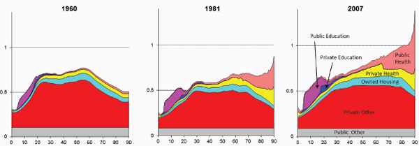
FIGURE 3-10 The age profile of U.S. consumption, 1960, 1981, and 2007. For each year, all values have been divided by average labor income in that year between ages 30–49 to standardize for visual comparison of shapes. SOURCE: Special tabulations by Lee and Donehower using data from the National Transfer Accounts project; see Lee and Mason (2011, Chapter 9) for details and methods.
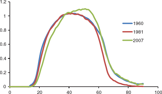
FIGURE 3-11 U.S. labor income by age, 1960, 1981, and 2007. Labor income is before taxes and includes fringe benefits and two-thirds of self-employment income. For each year, all values have been divided by average labor income in that year between ages 30 and 49. SOURCE: Special tabulations by Lee and Donehower using data from the National Transfer Accounts project; see Lee and Mason (2011, Chapter 9) for details and methods.
owing to the decline in “Private Other” spending—that is, all household consumption other than health, education, and services from owned housing. This predated Medicare and Medicaid, and public expenditures on health care were no greater for elderly individuals than for younger adults. By 1981, “Private Other” consumption did not begin to decline until age 70. Private spending on health rose substantially with age, and public spending on health care rose even more strongly with age. Total consumption rose across adult ages in 1981 in contrast to its decline in 1960, and rose strongly after age 85.
By 2007 these changes had intensified. Private nonhealth consumption did not decline until age 80 in 2007 as compared with age 70 in 1981 and age 60 in 1960. Most striking was the expansion of public spending on health care. We also see a sharp reduction in private spending on health care at age 65 and a corresponding increase in public spending through Medicare. Total consumption is now seen to rise strongly with age. In 1960 an 80-year-old consumed 83 percent of what a 20-year-old consumed. By 1981 an 80-year-old consumed 39 percent more than a 20-year-old, and by 2007 an 80-year-old consumed 67 percent more. The ratio of consumption at age 80 to age 20 doubled since 1960.
Comparable estimates are available for labor income (Figure 3-11). In 1960 and 1981, the labor income curve for the 20s and early 30s is shifted
3 to 4 years toward younger age relative to the curve for 2007. The 1960 and 1981 curves are virtually identical until age 60. After age 60, the 1960 curve is virtually coincident with the 2007 curve and is shifted 2 to 3 years toward older ages relative to 1981. In the 70s age range it is shifted many years toward older ages.4 The result of these changes in the economic life cycle is that consumption in old age net of labor income has become much more costly. Population aging will occur rapidly over the coming decades as the baby boom moves into older ages, and the societal costs will be heightened by the corresponding increase in the net consumption of the elderly. At the same time, the elderly in the United States continue to earn a substantial amount of labor income, more than in most other industrial nations (Lee and Mason, 2011).
INDICATORS OF POPULATION AGING
AND ITS ECONOMIC IMPACT
Demographers and economists use a range of indicators to compare the degree of population aging over time and between countries. The most basic of these measures can be calculated for all countries but have shortcomings that limit their usefulness; the more complex ones require more detailed data but are better suited to analyses of the economic impact of aging. One key point is that the correspondence between chronological age on the one hand and health and vitality on the other has changed dramatically in recent decades, as reflected in the popular saying “70 is the new 60.” These changes will be discussed in the next chapter, and must be kept in mind even as “the elderly” continue to be defined as people aged 65 and over.
Proportion of Population Aged 65 and Over
In 2010, 13 percent of the U.S. population was over the age of 64, up from 8 percent in 1950. This proportion is expected to jump above 20 percent over the next two decades as the baby boom generation retires, before plateauing in the 2030s and 2040s (Figure 3-12). The proportions aged 75+ and 85+ follow a similar path but at a lower level. Moreover, the upswings occur later, with a delay of 10 years for the 75+ population and 20 years for the 85+ population.
_______________
4Throughout this discussion of consumption and labor income we are comparing values across ages in the same time period. Actual paths of earning and consuming over the lifetime of a generation would have different shapes, tilted upwards and shifted to older ages, because productivity growth leads to growing income and consumption as generations move through their lives.
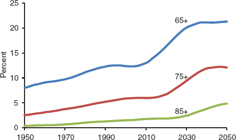
FIGURE 3-12 Share of population aged 65+, 75+, and 85+, 1950–2050. SOURCES: Board of Trustees, Federal Old-Age and Survivors Insurance and Federal Disability Insurance Trust Funds (2011) and projections by the committee.
Age Dependency Ratio
The age dependency ratio (ADR) is the ratio of population aged 65 and over plus those under 20 (“dependents”) to the working age population (ages 20–64). Figure 3-13 plots estimates of the ADR for the United States from 1950 to 2010 and projections to 2050. The ADR fluctuates substantially over time but shows no clear long-range trend. It reached its
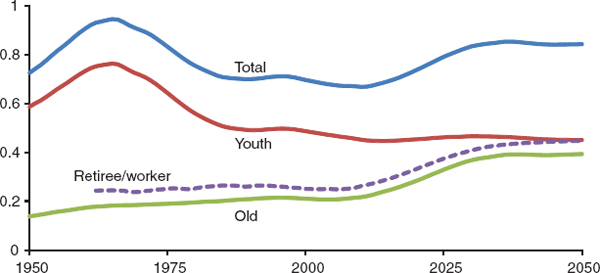
FIGURE 3-13 Age dependency ratios, 1950–2050. SOURCES: Board of Trustees, Federal Old-Age and Survivors Insurance and Federal Disability Insurance Trust Funds (2011) and projections by the committee.
peak value, 0.94, in 1965 then declined to its minimum, 0.67, in 2010 and is projected to rise again to a new peak, 0.85, in 2037.
To explain this trend it is useful to examine the two components of the ADR: the old age dependency ratio (OADR, population 65+/population 20–64) and the young age dependency ratio (YADR, population <20/ population 20–64). As seen in Figure 3-13, these two components show very different trajectories over time. The YADR peak in 1965 was responsible for the first peak in the ADR, and the future rise in the OADR is responsible for the projected second peak in the ADR in the 2030s. As a result of these opposing trends in the OADR and YADR, the composition of dependents shifts from mostly under age 20 in the 1960s to nearly even between old and young dependents in 2050.
Although widely used, this ratio has a key flaw: It implicitly assumes that all people aged under 20 and over 64 are “dependents” and that all people aged 20–64 are “working.” These assumptions are at best an approximation of reality, and the quality of this approximation changes over time both because of changes in actual economic behavior and because of changes in underlying health.
Retiree to Worker Ratio
The retiree/worker ratio (RWR) can be considered an improved version of the old age dependency ratio. The numerator of the RWR consists of the number of retirees (instead of the population 65+) and its denominator consists of all people in the labor force (instead of the population aged 20–64). The RWR typically exceeds the OADR by a small amount because the number of retirees exceeds the population aged 65+ and because the number of workers is somewhat smaller than the population aged 20–64. The trends over time in the two indicators are similar, as shown in Figure 3-13, where the dashed line represents the RWR.
Support Ratio
Unweighted
Support ratios differ from dependency ratios in that the supporters (or workers) are in the numerator and the dependents (or consumers) are in the denominator; these measures are therefore inversely related to dependency ratios. The simplest support ratio is the proportion of the population that is working. The numerator consists of everyone in the labor force5 and the denominator equals the entire population, all of whom are consumers. The
_______________
unweighted support ratio (SRU) rose from 1962 to 1980 then plateaued until 2010, but it is expected to decline by 2050 (Figure 3-14). The disadvantage of this measure is that it assumes that workers of all ages have equal incomes and that the same amount is consumed by people of all ages.
Weighted
The weighted support ratio (SRW) is a more sophisticated measure that improves on the unweighted version by allowing incomes of workers and consumption levels to vary by age. Specifically, the age patterns of consumption and labor income discussed previously (see Figure 3-10) are applied to the population by age to calculate the SRW. The ratio depends on the base year age profiles of consumption and labor income that are used. These are held constant to isolate the effect of changing population age distributions. It is a hypothetical “other things equal” calculation, not an attempt to project what the future ratios of labor income to consumption will be.
Trends and projections of SRW are presented in Figure 3-14 (top line), based on the labor income and consumption profiles of 2007 combined with each year’s population age distribution. The SRW is higher than the SRU mainly because income substantially exceeds consumption among
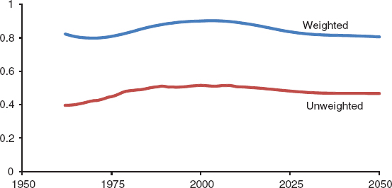
FIGURE 3-14 Unweighted and weighted support ratios, 1962–2050. SOURCES: Board of Trustees, Federal Old-Age and Survivors Insurance and Federal Disability Insurance Trust Funds (2011); Lee and Mason, 2011; and projections by the committee.
workers.6 However the pattern of change in the SRW over time is similar to that of the SRU.
Table 3-5 summarizes estimates of six indicators in 2010 and 2050. These aging indicators differ because they are differently defined. Their absolute levels will not be examined here because there is little to be gained from a discussion of the differences. Instead the committee focuses on the projected trends (last column), which anticipate the future impact of population aging.
These results lead to two main conclusions regarding trends to 2050. First, the U.S. population will likely age substantially, as indicated by the 64 percent rise in the population aged 65+, the 81 percent rise in the OADR, and the 71 percent rise in the RWR. Second, the economic impact of this aging is cushioned by a decline in youth dependency.
The net effect of these demographic trends is best captured by the SRW, which is projected to decline 12 percent by 2050. This means that, other things being equal, consumption per capita will be 12 percent lower than it would be without population aging.7
Adapting to Population Aging
As noted throughout this report, adapting to future population aging might involve a rise in the age at retirement. Such an increase would counteract the projected adverse changes in most of the above indicators. To illustrate, Figure 3-15 plots the age at retirement (conventionally set at age 65) required to keep the OADR constant at 0.22. This calculation indicates that the age at retirement would have to rise from 65.0 in 2010 to 73.3 years in 2050 to prevent the OADR from increasing. A separate calculation indicates that a similar increase in age at retirement will keep the SRW constant. It should be emphasized that Figure 3-15 represents a purely hypothetical exercise to illustrate the magnitude of changes in age at retirement needed to keep this dependency ratio unchanged. Such a large change in age at retirement is likely to be politically unacceptable, and it is not the committee’s intention to recommend it.
It is worth noting that this increase in the age at retirement of 8.3 years is larger than the rise of 4.0 years needed to keep the ratio of retired to working years constant over the individual life cycle (see earlier discussion of Figure 3-4). The reason for this difference is that the rise in the age at retirement plotted in Figure 3-15 compensates both for the projected rise in life expectancy and for population aging resulting from fertility decline
_______________
6The support ratio is typically less than unity because consumption is funded in part from sources other than labor income, such as asset income.
7That is, consumption per weighted consumer will decline by 12 percent, other things equal.
TABLE 3-5 Summary Indicators of Population Aging, 2010 and 2050
| Indicator | 2010 | 2050 | Percent Change, 2010–2050 |
| Aged 65+ (%) | 13.0 | 21.3 | 64 |
| ADR | .67 | .84 | 26 |
| OADR | .22 | .39 | 81 |
| RWR | .26 | .45 | 71 |
| SRU | .51 | .47 | −8 |
| SRW | .78 | .68 | −12 |
SOURCES: Board of Trustees, Federal Old-Age and Survivors Insurance and Federal Disability Insurance Trust Funds (2011) and projections by the Committee.
and migration changes. In contrast, the life cycle calculations summarized in Figure 3-4 compensate only for rising life expectancy.
GLOBAL PATTERNS OF AGING
Population aging is occurring in most countries because life expectancy has risen and fertility has declined. Aging is most pronounced in high-income countries (i.e., Europe, North America, and Japan), where the median age of the population rose from 29 to 39 years between 1950 and 2010 (United Nations, 2011). United Nations projections expect this median to reach 48 years in 2050. Populations in the developing world (Asia excluding Japan, Latin America, and Africa) are generally younger, with
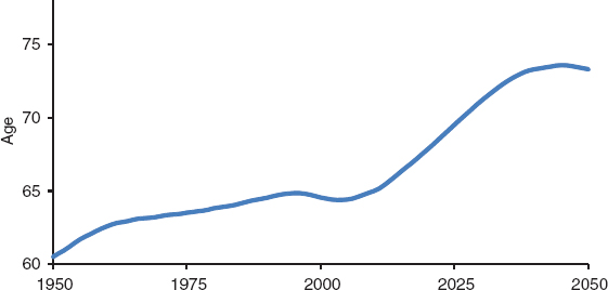
FIGURE 3-15 Retirement age required to keep old-age dependency ratio constant at its 2010 level. SOURCES: Board of Trustees, Federal Old-Age and Survivors Insurance and Federal Disability Insurance Trust Funds (2011) and projections by the committee.
a current aggregate median age of 27 years, but aging is also proceeding rapidly and the median is projected to reach 37 years in 2050.
Figure 3-16 plots past estimates and projections of the proportion aged 65+ for each of the world regions. Large regional differences are apparent. In 2010, proportions 65+ in Europe (16.2) and North America (13.2) are substantially higher than in Latin America (6.9), Asia (6.7) and Africa (3.5). By 2050 these proportions are expected to have risen further, reaching 26.9 percent in Europe and 21.6 percent in North America. The steepest increases are projected for Asia and Latin America, where levels will more than double and reach above today’s European levels. Africa will also age, but slowly, and will remain the youngest region.
Figure 3-17 compares the United States with other high-income countries. By mid-century the proportion aged 65+ is projected to reach 21 percent in the United States and substantially higher in other rich countries (over 30 percent in Germany, Italy, and Spain and 36 percent in Japan). The reason for this difference is the relatively high fertility in the United States and the low fertility in Germany, Italy, Japan, and Spain. In addition, the United States is expected to have higher mortality and migration rates. Other high-income countries therefore face more pronounced aging than does the United States.
UNCERTAINTY IN POPULATION PROJECTIONS
It is obvious that many assumptions are required for a population projection. Painful actions such as raising the retirement age might be taken
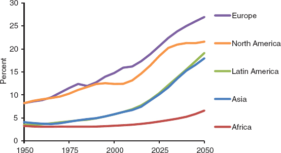
FIGURE 3-16 Share of the population aged 65+ in five world regions, 1950–2050. SOURCE: United Nations (2011).
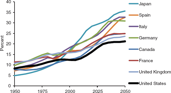
FIGURE 3-17 Share of population aged 65+ in eight high-income countries, 1950–2050. SOURCE: United Nations (2011).
now to ameliorate the consequences of projected population change far in the future. How certain can we be that the projected changes will actually occur and that action is needed now? To answer this important question, we need an indication of the uncertainty in the projections.
Demographers and statisticians have mainly used four different methods to assess the uncertainty of population projections (see National Research Council, 2000, for a detailed examination of both the accuracy of past projections and the uncertainty of population forecasts). The traditional method, which can be called “scenarios,” is familiar to all: The projections are made in high, medium, and low variants, based on expert opinion about how high or low each of the key inputs—fertility, mortality, and net immigration—might be. This is certainly helpful, but there are difficulties with this approach. It seems to assume that if fertility (for example) is higher than expected in the first year of the projection, then it will also be higher in every subsequent year, and this assumption rules out the kinds of fluctuations that have occurred in the past. Because of this, the scenario method invites us to believe that if we just wait for a few years it will become clear whether the population is evolving according to the high or the low scenario, and uncertainty will be reduced. But this interpretation is mistaken. After a few years, a new set of scenarios would again feature similar high, medium, and low variants.
Construction of the scenarios also requires deciding whether to combine the high fertility assumption with a low mortality assumption or a high mortality assumption, and likewise for migration assumptions. This
decision is essentially arbitrary, and however it is done, inconsistencies in the high-low ranges will result (see Lee, 1999).8
A second approach, called ex post analysis, analyzes the past record of success of forecasts prepared by an agency as a guide to the uncertainty of future forecasts. If the forecasting method has not changed too much over time, this method can be very useful. An unusually careful ex post analysis of the United Nations projections was provided by the National Research Council (2000).
A third approach might be called “random scenarios.” It assumes a certain probability distribution of the true outcome in relation to high and low bounds provided by experts. Given this distribution, a process like the one described above can be used to generate possible future paths for each vital rate (Lutz, Sanderson, and Scherbov, 2004; Tuljapurkar, Li, and Boe, 2000).
A fourth approach is based on time-series analysis, which combines demographic methods with well-established statistical methods to model, analyze, and forecast historical data on fertility, mortality or migration (Lee and Tuljapurkar, 1994). The models capture not only the trend but also the typical patterns and degree of persistence of fluctuations. One can draw random numbers that, combined with the models, generate one possible version of the future of a particular rate—say fertility—that is consistent with the typical past patterns (Lee, 1999; 2011). In the same way, possible futures can be generated for mortality and net immigration. Then this set of randomly generated fertility, mortality, and migration outcomes can be used to generate a possible future trajectory for the population and its age distribution, say up to 2050. By repeating this process with a new set of random numbers, another possible future is generated. After 1,000 such repetitions, it becomes clear which outcomes are most likely and which are less likely, and it is possible to derive a probability distribution. This method produces not only a probability distribution of outcomes for a given year, but also a distribution of trajectories. Such an approach is valuable because some outcomes of interest, such as the projected Trust Fund balance for Social Security in a given year, depend not only on the demography of that particular year but also on the whole demographic trajectory leading up to that point, with all its ups and downs. In fact, the Social Security Trustees have included in their annual reports a stochastic forecast of this sort for the system’s finances.
Figure 3-18 shows a probabilistic forecast of the OADR based on a stochastic version of the committee’s single-sex population projection, for
_______________
8In effect, the scenario method assumes that projection errors in each component are perfectly correlated over time (always too high or always too low), and that errors in the different components are always perfectly positively or negatively correlated with one another (if fertility is high, then mortality or immigration is low, for example). Neither assumption is correct.
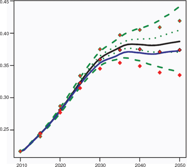
FIGURE 3-18 Old-age dependency ratio as projected by the committee, the Census Bureau, and the Social Security Trustees, 2010–2050. The central black line is the median committee forecast. There is a 50 percent probability that the ratio will lie between the green dotted lines in any year and a 95 percent probability that it will lie between the green dashed lines. The solid purple line is the 2008 Census Bureau projection. The red diamonds indicate the high, intermediate, and low variants of the 2012 Social Security Trustees projection. SOURCES: Donehower and Boe (2012), U.S. Census Bureau (2008), and Board of Trustees, Federal Old-Age and Survivors Insurance and Federal Disability Insurance Trust Funds (2012).
which 1,000 stochastic trajectories were created (see Appendix A for a description of the method used). The solid black line is the median in each year of the 1,000 random trajectories. The inner dotted green lines indicate quartiles, so there is a 50 percent chance that the future outcome will lie between them in a given year. The outer dashed green lines represent the upper and lower 2.5 percent bounds and define the 95 percent probability interval for the OADR in each year.
Figure 3-18 also plots the most recent Census Bureau projection of the OADR as a purple line. It is just at or below the lower 25 percent bound of the committee forecast, perhaps because the life expectancy forecast in the Census Bureau projection is lower than in the committee’s. The Census projection does not come with a range. Figure 3-18 further shows the OADR as projected by the Social Security Trustees in its 2012 high, intermediate, and low-cost variants, all indicated by diamonds. The intermediate projection is very close to the committee’s median through 2030, and then transits to the Census Bureau projection at the lower 25 percent of the committee’s range. The Trustees’ low-cost scenario is slightly below the lower 2.5 percent bound for the committee’s forecast, while the high-cost scenario rises above the committee’s upper 2.5 bound before dipping below this bound around 2040. The Trustees’ projection is centered a bit lower than the committee’s owing to less projected gain in longevity (life expectancy of 82.2 years in 2050, versus the committee projection of 84.5 years, as discussed earlier). The Trustees do not assign a probability to the range for the OADR, but Figure 3-18 suggests that its probability coverage is about 95 percent. This is the probability that the OADR in any given year will fall between the high-cost and low-cost brackets. This does not mean, however, that there is a 5 percent chance that the OADR would generally lie outside this range in every year between 2010 and 2050. That probability would be far lower, because a typical trajectory of the OADR would wander around within that range, with offsetting upward and downward variations.
This last point can be seen clearly in Figure 3-19, which shows a probabilistic forecast of the weighted support ratio based on the age profiles for 2007 shown earlier in Figures 3-10 and 3-11. It uses the same 1,000 stochastic trajectories and plots 20 of them for illustrative purposes. The trajectories often can be seen to fluctuate rather than to be persistently high or low. As in Figure 3-18, the solid black line is the median projection. The dashed blue lines indicate quartiles (so there is a 50 percent chance that the future outcome will lie between them in a given year), and the dashed green lines represent the upper and lower 2.5 percent bounds and define the 95 percent probability interval. The value of the ratios has been adjusted so that the ratio in 2007 is 1.0. That is, the plotted values show the ratio relative to the ratio in 2007.9
The expected decline in the support ratio between 2010 and 2050 is 12 percent (the same as reported earlier in this chapter), and there is a two-
_______________
9Of course, the age profiles of labor income and consumption will change over the next four decades, and any attempt to project their future levels would involve substantial uncertainty. However, the support ratio for future years is calculated using the baseline (2007) age profiles so as to isolate the effects of demographic change. Therefore the uncertainty surrounding future values of the age profiles is irrelevant. For a discussion of the construction and use of support ratios in this context, see Cutler et al. (1990).
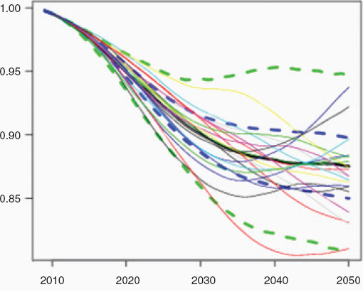
FIGURE 3-19 Projected weighted support ratio with probability bounds and 20 illustrative stochastic trajectories, 2010–2050. The central dark line is the median committee forecast. There is a 50 percent probability that the support ratio will lie between the blue dashed lines in future years and a 95 percent probability that it will lie between the green dashed lines. The figure shows 20 trajectories. The actual projection is based on 1,000 sample paths. For the method used, see Appendix A. SOURCE: Donehower and Boe (2012).
thirds chance that the decline will be between 9 percent and 16 percent, and a 95 percent chance that it will be between 5 percent and 19 percent. We can conclude from the stochastic approach in Figures 3-18 and 3-19 that it is virtually certain that the U.S. will experience substantial population aging and that the support ratio is virtually certain to fall in the coming decades. The expected decline of 12 percent translates into an average yearly rate of decline of one-third of 1 percent (0.33 percent).


