
THE SUN AND SOLAR VARIABILITY—PAST AND PRESENT
Over the past 30 years substantial advances have been made in understanding variability in solar output. Perhaps most dramatic has been the improved insight into the classic question posed by William Herschel two centuries ago: Does the Sun’s brightness vary?1 Information on total solar irradiance (TSI) behavior has advanced from inferential knowledge for times prior to 1980 to the current understanding of its variation on scales from minutes to the 11-year cycle.
Solar variability is closely related to the structure and magnitude of the solar magnetic field, and so the ability to reconstruct past solar outputs, or predict them, is only as good as the understanding of how the solar magnetic field varies in time and location on the Sun. The past 20 years have seen great strides in the ability to model the large- and smaller-scale structure and variability of the solar magnetic field.2 These developments in models have been supported by the ability to make measurements of the solar magnetic field.
Precise helioseismic measurements reveal the complex depth dependence of solar rotation throughout the convection zone and well into the radiative core. However, translation of these advances into improved understanding of the dynamo processes that generate solar magnetism has proven more difficult.3 There is still no precise predictive model of the dynamo that drives solar magnetism over the 11-year cycle or of its modulation envelope over centuries and millennia.
The most rapid advances in this area are coming from simulations of magneto-convection on small scales in relatively shallow layers.4,5 Their extension to the much deeper layers of the convective and tachocline zones that are most likely to generate the 11-year sunspot cycle is not yet possible with today’s computing power.
At the September 2011 workshop, presentations on this topic included discussions of advances in solar radiometry, an assessment of solar influences on Earth’s climate change, heliospheric phenomena responsible for cosmic ray modulation, and the behavior of quiet Sun contributions to solar irradiance on timescales ranging from years to thousands of years.
_______________
1 W. Herschel, Observations tending to investigate the nature of the Sun, Philosophical Transactions of the Royal Society of London 91:265-318, 1801.
2 Y.-M. Wang, A.G. Nash, N.R. Sheeley Jr., Magnetic flux transport on the Sun, Science 245:712, 1989.
3 P. Foukal, Solar Astrophysics, Wiley Online Library, 2nd edition, available at http://onlinelibrary.wiley.com/doi/10.1002/9783527602551.fmatter/summary, 2004.
4 M. Carlsson, R.F. Stein, A. Nordlund, and G.B. Scharmer, Observational manifestations of solar magnetoconvection: Center-to-limb variation, Astrophysical Journal Letters 610:137, 2004.
5 M. Rempel, Penumbral fine structure and driving mechanism of large-scale flows in simulated sunspots, The Astrophysical Journal 729(1):5, 2011.
Overview and Advances in Radiometry for Solar Observations
Greg Kopp, University of Colorado, Boulder
Greg Kopp began by listing the potential climate-relevant changes in Earth’s radiation budget ranging from volcanic dust veils to heating from radioactive decay in Earth’s interior. Solar irradiance is the dominant energy source for Earth, four orders of magnitude greater than the next largest contributor, radioactive decay. Although the Sun’s irradiance can change significantly during the passage of features on its surface, such changes are of sufficiently high frequency as to not affect climate. More relevant are trends of a decade or longer. As Kopp explained it, the challenge is to delineate these longer-term solar changes and to discriminate them from other causes of climate change. Statistical studies have suggested that natural influences—including the Sun, effects from volcanic eruptions, and changes in Earth-atmosphere-ocean coupling—together explain roughly 15 percent of the past century’s temperature anomaly. Although small, the contribution from the Sun must be determined with a high degree of accuracy in order to reliably quantify the other contributors to climate change (Figure 2.1).
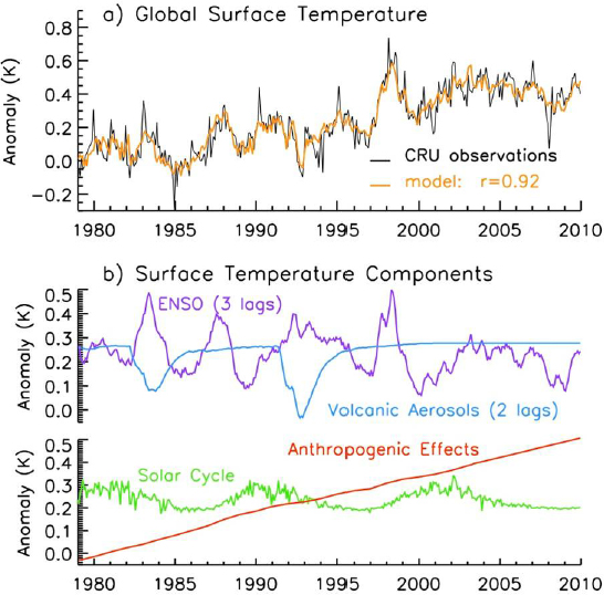
FIGURE 2.1 Global temperature and surface temperature components of Earth’s climate. Combined El Niño-So0uthern Oscillation (ENSO), volcanic aerosols, solar activity, and anthropogenic effects explain 85 percent of observed temperature variance. SOURCE: G. Kopp and J.L. Lean, A new, lower value of total solar irradiance: Evidence and climate significance, Geophysical Research Letters 38:L01706, 2011; Copyright 2011 American Geophysical Union, reproduced by permission of American Geophysical Union.
The Sun may vary by as much as 0.1 percent over the 11-year solar cycle and perhaps by 0.05 to 0.3 percent over centennial timescales. Uncertainty in the long-term variability is limited by the proxy models used to derive irradiance backward in time, before the measurement record began. Kopp used an estimate of how the Sun might have varied coming out of the Maunder Minimum, by approximately 0.1 percent over 80 years, to derive accuracy and stability requirements for measuring TSI. Although change of that magnitude may be easy to measure over a solar rotation or over a maximum-to-minimum half solar cycle, it is a considerable challenge to derive a change that small over a century. This derivation requires a stability of 10 parts per million (which is at the frontier of the possible with the best instruments today), and it requires substantial periods of overlap between those measurements with different instruments and a long-term accuracy of 100 parts per million. These tight demands make it difficult to obtain such measurements needed for climate science. To resolve the offsets among the various measurements of TSI that make up the 33-year record, Kopp and his colleagues established a test facility using a calibrated cryogenic radiometer and a laser source at solar power levels to provide the first-ever end-to-end validation of active cavity solar irradiance instruments. This facility also helped resolve the source of the offsets among the various TSI instruments. For the Solar Radiation and Climate Experiment (SORCE) Total Irradiance Monitor (TIM) the precision aperture is at the front of the instrument. All of the other sensors use view-limiting apertures in front of the precision aperture. By overfilling and underfilling that aperture, Kopp determined that scattered light was the source of a large fraction of the offsets between those instruments and SORCE TIM, which measures a TSI of approximately 1361 W m-2, the lowest among the group (see Figure 1.1 in Chapter 1). The scattering-corrected Active Cavity Radiometer Irradiance Monitor (ACRIM) measurements are now very close to this value, as are those from Precision Monitoring Sensor (PREMOS). A large scattering correction was derived for the Variability of Solar Irradiance and Gravity Oscillations (VIRGO) instrument, but it has yet to be applied.
Although the general agreement among the ACRIM, PREMOS, and TIM instruments has improved since the discovery of scattered light in the ACRIM and PREMOS sensors, Kopp showed that only the TIM is accurate (100 ppm) and stable (10 ppm per year) enough to monitor the long-term changes of the Sun at climate-quality levels on timescales of years to decades. Without this level of stability it is difficult to distinguish real solar change (for example, between successive solar minima) over instrument drift. Thus, Kopp concluded, it is crucial that the TSI record from TIM remains unbroken, a proposition growing riskier with time since the failure of the Glory launch in 2011, and one that now must rely on overlap between SORCE and the Total Solar Irradiance Sensor.
Assessing Solar and Solar-Terrestrial Influences as a Component of Earth’s Climate Change Picture
Daniel N. Baker, University of Colorado, Boulder
Given the previous discussion there are then two challenges: understanding the variation in TSI in the modern era and extrapolating back in time on the order of tens of millennia to understand the variation in TSI through the use of proxies. Baker pointed out that measurements of total solar irradiance vary widely, and the normalization of the values could possibly obscure small trends—a problem he feels should be addressed. Historical TSI reconstruction connects these contemporary TSI measurements via an index that requires extrapolating the TSI back in time—with the attendant uncertainties. As Baker summarized, the connection between TSI and various proxies is that the size of the heliosphere controls the number of galactic cosmic rays (GCRs) that reach Earth: the GCR flux is higher at solar minimum. Isotopic abundances in the atmosphere are altered by GCR flux, generating increased 14C and 10Be, and this isotopic evidence is found in tree rings and ice cores.
Baker also noted that GCRs reach into the stratosphere and troposphere, and are an important “top-down” mechanism for coupling the Sun to climate. For example, Lockwood et al. found a
correlation between GCR and TSI,6 and Russell et al. presented a discussion of the link between the modulated energetic particle flux and nitrogen oxide production in the stratosphere showing a link to ozone.7 The destruction of ozone changes the energy balance in the atmosphere because ozone absorbs solar radiation. Baker discussed how Randall et al. quantified this in terms of the trend in ozone using the WACCM general circulation model that includes the upper-atmosphere dynamics and chemistry.8 The high-latitude case shows a depletion of stratospheric ozone due to increases in nitrogen oxides from energetic particles that then is reflected in a lower-atmosphere increase in ozone due to destruction of chlorine oxide through reactions with nitrogen oxides. Baker concluded, however, that all of these processes appear to have a minimal effect on surface temperatures.
Behavior of Quiet Sun Contributions to Solar Irradiance
Peter Foukal, Heliophysics, Inc.
The main aim of Peter Foukal’s presentation was to consider whether the Sun dimmed enough during the 17th century Maunder Minimum of solar activity to influence climate. He argued that the simplest way to achieve sufficient dimming is through a decline in the area coverage of small flux tubes in the quiet magnetic network and internetwork (Figure 2.2).
The fractional decline required may be less than the complete disappearance required by earlier irradiance models, judging by recent findings from solar photometry. These findings9 indicate that the excess radiative flux/unit area of faculae increases with their decreasing cross section. This relationship suggests that climatically significant variations in TSI might be achieved without the need for the complete disappearance of photospheric magnetism. Foukal noted that this relationship is important because 10Be proxy record studies indicate persistence of a residual 11-year solar cycle through the Maunder Minimum.
Foukal then pointed out that present estimates of the quiet network’s contribution to total irradiance (Figure 2.3) are uncertain because of limitations on angular resolution, angular coverage, or wavelength coverage. He described how, ideally, the measurement should be carried out with the Solar Bolometric Imager, which has been flown by the Johns Hopkins University Applied Physics Laboratory on NASA balloons,10 but modified for larger image scale and higher angular resolution.
If the contribution of the quiet network to TSI is significant, it is still necessary to know whether the network’s area decayed. This decay is controversial,11 but the most reproducible indices of network area (such as MgII) did indicate a decline by 5-10 percent below the average of previous minimum values, during the most recent 2008-2009 activity minimum.12 This amount of decline during a minimum that was only about 1 year longer than normal suggests an even greater decline during a Maunder
_______________
6 M. Lockwood, What do cosmogenic isotopes tell us about past solar forcing of climate? Space Science Review 125:95-109, 2005.
7 J.M. Russell, S. Solomon, L.L. Gordley, E.E. Remsberg, and L.B. Callis, The variability of stratospheric and mesospheric NO2 in the polar winter night observed by LIMS, Journal of Geophysical Research 89:7267-7275, 1984.
8 C. Randall, E.D. Peck, L.A. Holt, V. Harvey, D.R. Marsh, X. Fang, C.H. Jackman, M.J. Mills, and S.M. Bailey, Atmospheric coupling via energetic particle precipitation, paper presented at the American Geophysical Union Fall Meeting, December 13-17, 2010, San Francisco, Calif., 2010.
9 P. Foukal, A. Ortiz, and R. Schnerr, Dimming of the 17th Century Sun, The Astrophysical Journal Letters 733:L38, 2011.
10 P. Bernasconi, H.A.C. Eaton, P. Foukal, and D.M. Rust, The solar bolometric imager, Advances in Space Research 33:1746-1754, 2004.
11 C.J. Schrijver, W.C. Livingston, T.N. Woods, and R.A. Mewaldt, The minimal solar activity in 2008-2009 and its implications for long-term climate modeling, Geophysical Research Letters 38: L06701, 2011.
12 C. Frölich, Evidence of a long-term trend in total solar irradiance, Astronomy and Astrophysics 501: L27-L30, 2009.
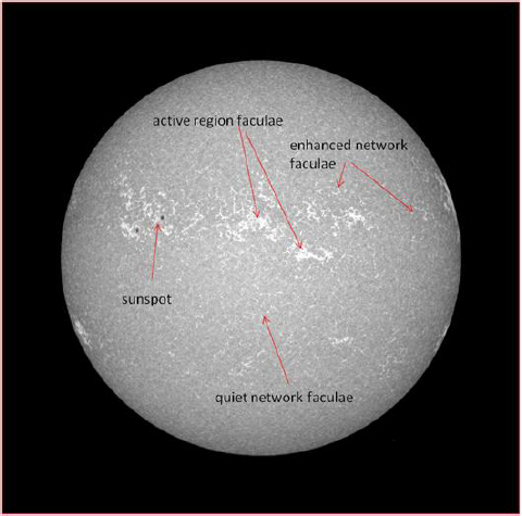
FIGURE 2.2 Image of the Sun’s upper photosphere in the 170 nm continuum showing the magnetic structures responsible variation in for total solar irradiance and in 130-240 nm ultraviolet irradiance. SOURCE: Courtesy of P. Foukal, Heliophysics, Inc.
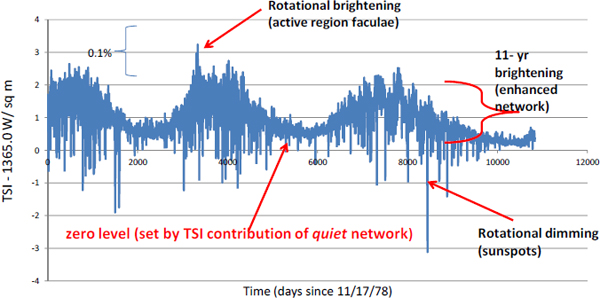
FIGURE 2.3 Variation in total solar irradiance (TSI) measured radiometrically (Physikalisch-Meteorologisches Observatorium Davos composite) between 1978 and the present, identifying the magnetic structures responsible for variation in TSI and the 130-240 nm ultraviolet irradiance. SOURCE: Courtesy of P. Foukal, Heliophysics, Inc.
Minimum-like episode lasting 70 years. Foukal asserted that further work is required on this network-area behavior during extended activity minima.
Foukal stressed that there is no evidence for the large (~0.3 percent) increase in TSI during the early 20th century reported in a recent, widely quoted, study based on 10Be.13 That level of increase in TSI would require the complete disappearance of the quiet network and internetwork going back in time to 1900. This requirement contradicts the presence of a fully developed network on Ca K spectroheliograms available since the 1890s.14 Foukal asserted that this model, which also predicts strong TSI driving of climate throughout the Holocene, cannot be correct.
Heliospheric Phenomena Responsible for Cosmic Ray Modulation at the Earth
Joe Giacalone, University of Arizona
Galactic cosmic rays are expected to be essentially isotropic in the space immediately outside the heliosphere and penetrate the solar system with nearly equal probability from all directions. As GCRs enter the solar system, they undergo both energetic and intensity variations resulting from their interaction with the solar wind, interplanetary magnetic field, and the heliosphere (Figure 2.4). As Joe Giacalone discussed, GCRs interact with atomic nuclei in Earth’s atmosphere, creating a secondary cosmic ray (neutron) that can interact with a background very abundant in oxygen and nitrogen to form 14C or 10Be, among other nuclei. The GCR intensity at the top of Earth’s atmosphere is anti-correlated with the number of sunspots—GCR intensity is higher when there are fewer sunspots. This anti-correlation is the basis for using 14C and 10Be deposited in tree rings and ice cores as a proxy measure of solar activity dating back thousands of years. In addition to the 11-year GCR cycle, there is also a 22-year variation related to the polarity of the solar magnetic field. These variations can be understood through the physics of charged-particle motion in turbulent electric and magnetic fields associated with the solar wind plasma. Even during the Maunder Minimum when sunspots were scarce, there were still polarity reversals, and there were still enhancements of GCRs in the 11-year cycle such that a stronger magnetic field yielded smaller GCR flux. The highest flux of GCRs on record occurred during the most recent solar minimum.
The radioisotope record in 14C and 10Be provides information on the varying concentration of these isotopes in the biosphere over past millennia. This information can be translated into a time series showing the variation in flux of the GCRs mainly responsible for the formation of these isotopes. The resulting GCR flux variation has been used in Sun-climate studies in two separate ways. It can be used directly to study the possible effect of GCR variation on atmospheric electrification and cloud formation. As pointed out in the presentation by Giacalone, recent findings from laboratory measurements at CERN have brought more attention to studies of cosmic ray effects. He also described the various influences causing GCR flux variation on timescales from days to millennia. Sudden changes in the solar magnetic field or in the resulting heliospheric structures account for the rapid changes. The 11- and 22-year cycles are caused by more gradual variation of the heliospheric field strength and complexity, and in the number of solar eruptive events over the sunspot cycle. Supernova eruptions and other changes in the interstellar medium play a role on millennial timescales because of the large distances between stars and the diffusive transport of the GCR population. Nearby supernovae can create short-lived pulses, but these are exceptionally rare.
_______________
13 A. Shapiro, W. Schmutz, E. Rozanov, M. Schoell, M. Haberreiter, A.V. Shapiro, and S. Nyeki, A new approach to the long-term reconstruction of the solar irradiance leads to large historical solar forcing. Astronomy and Astrophysics 529:67, 2011.
14 P. Foukal, A new look at solar irradiance variation, Solar Physics 279:365-381, 2012.
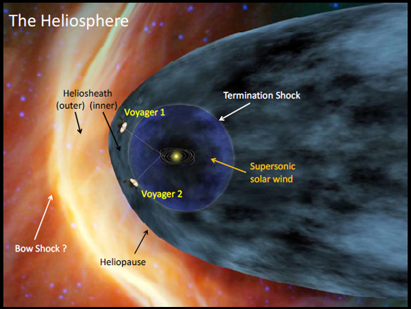
FIGURE 2.4 Diagram of the heliosphere. SOURCE: Courtesy of J. Giacalone, University of Arizona, modified from NASA image available at http://www.nasa.gov/mission_pages/sunearth/multimedia/Heliosphere.html, courtesy of NASA/Goddard/Walt Feimer.
Giacalone also pointed out that, although the four basic processes of particle diffusion, convection, drifts, and energy changes have been known for 50 years, the transport coefficients needed to calculate their effects are still poorly known. However, it is now accepted that none of the processes included in the classic Parker transport equation can be neglected; it is a complex system. This complexity limits the accuracy of attempts to use the isotope record to derive the record of solar irradiance. The solar modulation of cosmic rays is caused by both the relatively gradual evolution in the background solar wind and by the pulses associated with coronal eruptions, through the complex processes referred to. Much of the variation in irradiance (at least the 11-year variation) originates from the emission from plasma heated by the dynamics of the near-surface magnetic field with contributions from both the open and closed field components both during quiescence and during flarings. This differential behavior makes it difficult to use radioisotopes to generate more than a rough estimate of variation in TSI and ultraviolet flux, such as those shown by workshop presenter Raimund Muscheler.
Giacalone showed the evidence for a low-level 11-year cycle in radioisotopes during the extended Maunder Minimum of solar activity during the 17th century. Such isotopic evidence currently provides the best chance of determining how much the solar magnetic field decreased during that period and therefore how much the Sun dimmed. He discussed how the differences between galactic cosmic rays and anomalous cosmic rays (ACRs) could be seen during the most recent solar minimum. The GCR intensity was the highest measured by spacecraft, but ACRs had a lower intensity compared to previous solar minima. He suggested one possible interpretation was that fewer ACRs were being produced at the termination shock of the heliosphere. This difference is useful for determining the physics of cosmic ray transport in the heliosphere.
The Record of Solar Forcing in Cosmogenic Isotope Data
Raimund Muscheler, Lund University, Sweden
Muscheler discussed how information can be recovered about the Sun’s activity in the past from studies of cosmogenic isotope data. The most common isotopes used in these studies are 10Be in ice cores and 14C in tree rings, and they can be used together to separate changes in solar activity from differences in climate. He noted that responses in the data are seen not only for solar modulation but also for variations in Earth’s geomagnetic field on timescales longer than 500 years. The challenge is to detect reliable signals from these data sets for a particular time period. TSI can be considered to be more closely tied to the closed flux (which is larger than the open-field fraction) and magnetic features on the Sun compared to the modulation of the GCRs in the heliosphere by the Sun’s open flux. He noted that when talking about the cosmic-ray flux at Earth, Earth’s magnetic field determines where and how much of the cosmic -ray flux makes it into Earth’s atmosphere. An estimate of the geomagnetic field intensity is necessary along with isotope measurements to determine the solar modulation. In the atmosphere itself, circulation and climate also affect the deposition of the isotopes.
14C’s response to variations in the solar cycle is affected by the fact that the 14C is taken up in CO2. Muscheler explained that CO2 remains in the atmosphere for approximately 7-8 years and then has a long residence time in the large reservoir of the ocean where it can continue to exchange with the atmosphere and the biosphere before being trapped in tree rings. This leads to a dampening of the smaller-scale variations. Because of this residence time in a large reservoir, 14C is a less direct proxy for cosmic rays, but it does have the advantage of being less subject to concerns about geographic influences than is 10Be. 14C records a more global signal on 11-year-cycle timescales or longer. Muscheler stated that even if changes in climate cause changes in the carbon cycles of the biosphere and the ocean, the 14C in the atmosphere changes at the same rate and so does not obscure a solar signal. Even though climate influence is unlikely to be a major influence, a model of the carbon cycle is needed to calculate 14C production rates to make an assumption about the carbon cycle. Variations in 14C in the atmosphere alone do not provide a signal of the production of 14C.
Muscheler discussed how 10Be is produced by spallation processes in the atmosphere through reactions with nitrogen and oxygen. These reactions require high-energy particles. Normally energies at these levels are seen only in GCRs and in the relatively rare solar proton events (SPEs). These SPE contributions are relatively short-lived and are generally believed to be undetectable in the climatological record because they are obscured by other short cycles, such as the changes in 18O caused by yearly temperature changes.
Muscheler continued by explaining how 10Be is produced in the stratosphere, becomes attached to aerosols, and is then sensitive to stratosphere-troposphere exchange processes before being deposited and trapped in ice cores. 10Be is further complicated by the geomagnetic field configuration characteristic of the location. High-latitude locations such as Greenland or Antarctica have little shielding, and so the solar signal is relatively strong. At low latitudes there is little variation with solar cycle due to the stronger geomagnetic shielding. A still unresolved issue is how to go from a local measurement with some random variability to a globally representative value. Muscheler summarized 10Be as a relatively direct proxy for cosmic rays with significant noise associated with location and climate influences.
Muscheler discussed two commonly used data sets from the past 1,000 years for 10Be. Both sets of data show a largely consistent picture with the Maunder and Spörer Minima from activity indices seen in the 10Be record. There is a disagreement between researchers when looking at the records from the past 50 years. On the basis of one data set, it can be argued that today’s base solar activity is high, but that it is not unprecedented. Others claim that their reconstruction indicates a period of high solar activity in the past 60 years that is unique in the past 1,150 years. Muscheler suggested that the difference between the recent records is caused by one of them having been influenced by non-solar-related climate change. Muscheler discussed evidence of long-term changes in solar activity over the past 10,000 years. There are, however, uncertainties engendered by the comparison of the 10Be to the 14C record. These differences may be due to changes in 10Be transport, snow accumulation rates, carbon cycle uncertainties, or
geomagnetic field uncertainties. Muscheler stated that further research would be required to understand these differences.
Muscheler pointed out that there is good agreement between 10Be and 14C on the scale of the 11-, 88-, and 207-year solar cycles and that those signals can be clearly seen. On the other hand, there is no evidence of sustained periods on the order of 1,000 years of low solar activity in either the 10Be or the 14C record. This can be said with some confidence for the records going back over the past 10,000 years; however, characterization any farther back than that is more complicated because of the influence of climate change during the last ice age on the 10Be record.
In response to a question from the audience on the “climate/cosmic ray hypothesis” (i.e., that cosmic rays decreased over the last half of the 20th century and that this decrease is linked to the climate change of the past 30 years), Muscheler stated that proxy data indicate that the cosmic-ray flux actually decreased early in the 20th century, but recently the level has been steady and high. Based on the proposed link between increased GCR flux and cloudiness, one might have expected that the late 20th century would be cooler than the early 20th century—a state that was not observed.
Another audience member pointed out that it is necessary to be careful about the scale of the solar activity minima; minima on the scale of the heliosphere are not appropriately grouped with those on the scale of a hundred kilometers. The relationship between the large- and the small-scale field of the Sun is not known. Muscheler agreed that in his radionuclide data, only the solar modulation of GCRs can be clearly seen.
Solar Grand Minima Inferred from Observations of Sun-like Stars
Dan Lubin, Scripps Institution of Oceanography, University of California, San Diego
Dan Lubin discussed how the behavior of Sun-like stars can provide insight into the Sun’s activity and how solar forcing may change in the future. The frequency of grand minima (Maunder Minimum-like occurrences) is difficult to extract from the geophysical proxy record. In a sample of solar-type stars, the fraction of very inactive stars is analogous to the fraction of the Sun’s lifetime spent in a Maunder Minimum-like state. Early estimates of grand minimum frequency in solar-type stars ranged from 10 to 30 percent,15 implying that the Sun’s influence could be overpowering. It was later determined using much more accurate distance data from the European Space Agency’s Hipparcos Space Astrometry mission that these studies included many stars that evolved off the main sequence and are no longer burning hydrogen like the Sun.16,17 More recent studies, using the Hipparchos data and accounting for the metallicity of the star, place the estimate in the range of less than 3 percent for the fraction of the Sun’s lifetime spent in a Maunder Minimum-like state of low activity.18 The deduced frequency of occurrence of a Maunder Minimum state is sensitive to the choice of metallicity threshold and the definition of level corresponding to “inactive.”
Lubin pointed out that the early pre-Hipparcos estimates of Maunder Minimum analog frequency gave estimates that are too large. Instantaneous activity measurements of the hydrogen and potassium spectral lines (HK) are suggestive but not conclusive for identifying Maunder Minimum analog candidates; the result depends strongly on the chosen inactive threshold. Very low activity may be seen with an old star nearing the end of its main sequence lifetime. However, the historical Maunder Minimum most likely did involve very low HK activity and weak cycling compared with the present-day Sun.
_______________
15 S. Baliunas, and R. Jastrow, Evidence for long-term brightness changes of solar-type stars, Nature 348:520-523, 1990.
16 J.T. Wright, Do we know of any Maunder Minimum stars? The Astrophysics, Journal 128:1273, 2004.
17 P.G. Judge, and S.H. Saar, The outer solar atmosphere during the Maunder Minimum: A stellar perspective, The Astrophysics Journal 663:643, 2007.
18 D. Lubin, D. Tytler, and D. Kirkman, Frequency of Maunder minimum events in solar-type stars inferred from activity and metallicity observations, The Astrophysical Journal Letters 747: L32, 2012.
EVIDENCE OF SUN-CLIMATE CONNECTIONS ON DIFFERENT TIMESCALES
Instrument meteorological records rarely extend back more than 200 years; therefore, a long-term perspective on solar forcing must rely on the records provided by paleoclimate archives—principally, ice cores, lake and marine sediments, stalagmites, corals, and tree rings. Within each of these natural archives, a number of parameters can be measured and their relationship to climate assessed through calibrations with overlapping instrument data. In this way, paleoclimate proxies extend the record of past climate over past millennia.
Workshop presentations on this topic included discussions of detection of solar signals from paleorecords and temperature proxies as well as the role of cyclic and secular forcing at Earth’s surface and the corresponding climate response.
Detection of the Solar Signal in Climate from Paleorecords
Raymond S. Bradley, University of Massachusetts
Paleoclimate archives also provide an index of past solar activity, through the record of changes in cosmogenic isotopes recorded in tree rings and ice cores. In particular, variations in the cosmogenic isotopes 10Be and 14C indicate changes in the production rate of these isotopes. Raymond Bradley described how, over the past 12,000 years, these variations have been controlled mainly by changes in Earth’s magnetic field, and the field was weaker than today’s for much of that period (only ~40% of the present day value at 7000 years before present). Thus, isolating solar magnetic effects on the production rate of 10Be and 14C requires that changes in the geomagnetic field strength be removed, leaving the heliomagnetic signal as a residual. Unfortunately, past changes in Earth’s magnetic field are not well constrained, and Bradley indicated that further research on this topic is needed to refine the signal of whatever residual solar signal may be present. Furthermore, although attempts have been made to calibrate changes in 10Be in terms of variations in total solar irradiance,19 it is still debatable how variations in cosmogenic isotope production relate to changes in total or spectrally distributed irradiance.
Bradley noted that, despite these limitations, paleoclimatologists have generally accepted that the record of 10Be or 14C anomalies provides an index of changes in TSI, and have often sought to correlate paleoclimatic records with these data. The results have been mixed. In the case of the high-resolution Belukha glacier ice core data (from the Siberian Altai), a well-defined correlation between δ18O (a proxy for March-November mean temperature) and 10Be was found, with the strongest correlation associated with a 20-year lag in the temperature response.20 Furthermore, spectral analysis of the δ18O record revealed statistically significant variance at 10.8, 86, and 205 years, frequencies known to be prominent in the 14C anomaly record. However, when other nearby proxy records were examined, there was no evidence for a similar relationship to solar forcing, leaving open the question of whether the Belukha record is superior to the others, or whether the observed relationship is only of local significance.
Bradley discussed how a number of high-resolution ice core records have noted a strong relationship between 14C anomalies and changes in oxygen isotopes in the stalagmite carbonate. For example, Neff et al. noted a high correlation between δ18O in a stalagmite from Oman, and 14C, which they suggest is related to solar influences on monsoon-derived rainfall.21 Similarly, Wang et al. examine
_______________
19 See, for example, F. Steinhilber, J. Beer, and C. Fröhlich, Total solar irradiance during the Holocene, Geophysical Research Letters 36:L19704, 2009.
20 A. Eichler, S. Olivier, K. Henderson, A. Laube, J. Beer, T. Papina, H.W. Gäggeler, and M. Schwikowski, Temperature response in the Altai region lags solar forcing, Geophysical, Research, Letters 36: L01808, 2009.
21 U. Neff, S.J. Burns, A. Mangini, M. Mudelsee, D. Fleitmann, and A. Matter, Strong coherence between solar variability and the monsoon in Oman between 0 and 6 kyr ago, Nature 411:290-293, 2001.
δ18O in a well-dated monsoon-derived stalagmite from southern China and found a highly statistically significant relationship with 14C anomalies over the past ~9,000 years.22
Bradley asserted that it is noteworthy that all these studies focus on changes in the hydrological cycle of each region, rather than changes in temperature. This points to the possibility that if there is a solar effect on climate, it is manifested in terms of changes in the general circulation, rather than in a direct temperature signal. Bradley noted that in fact, despite the serious limitations in terms of statistical significance of most of the published paleoclimate studies that claim to find a solar signal in the records, there is nevertheless a clear geographical pattern in the overall signal that emerges when all records are mapped out. Specifically, periods of high cosmogenic isotope production (which might be related to reduced irradiance) appear to be associated with weaker monsoon rainfall in Oman, India, and southern China. There is also evidence for colder conditions at high latitudes, more extensive sea-ice in the North Atlantic, and wetter and colder conditions in western Europe, suggesting a general expansion of the polar vortex and a southward displacement of the westerlies when solar activity is low. There is a corresponding displacement, or seasonal shift in the intertropical convergence zone, affecting rainfall distribution in Central and South America and equatorial Africa.23,24,25 Meehl et al. suggested that this pattern results from regional differences in radiation receipts, with cloud-free zones differentially warming more than cloudy regions during periods of higher TSI, leading to changes in circulation patterns.26 Others have related solar-driven changes in stratospheric heating to changes in tropospheric circulation.27 Bradley concluded that either top-down or bottom-up effects (or both) may be relevant in explaining the pattern of hydrological changes that appear to be present in the paleoclimatic records. However, he asserted that it is clear that the current evidence for solar forcing from paleoclimate is very limited, and most records do not provide the necessary resolution or signal strength to detect a solar signal if it is present. Bradley suggested that further studies could be designed to address this question in a more rigorous and systematic manner.
Detecting the Solar Cycle Via Temperature Proxies Back to the Maunder Minimum
Gerald R. North, Texas A&M University
Gerald North described an approach to detection of a solar signal in 18O climate records thought to record air temperature at the time of deposition on snow/ice fields. Some of these records are claimed to resolve timescales fine enough to spectrally resolve signals at the 11-year-cycle period. North described efforts to do this in oxygen isotope data from the Dye-3 core from Greenland and the Taylor Dome cores from Antarctica, both of which revealed a weak 11-year signal. He described how further research, involving additional well-dated records and band pass filtering, may further elucidate the temporal evolution of such signals in relation to the long-term record of solar forcing.
_______________
22 Y. Wang, H. Cheng, R.L. Edwards, Y. He, X. Kong, Z. An, J. Wu, M.J. Kelly, C. A. Dykoski, and X. Li, The Holocene Asian Monsoon: Links to solar changes and North Atlantic climate, Science 308:854-857, 2005.
23 D.E. Black, L.C. Peterson, J.T. Overpeck, A. Kaplan, M.N. Evans, and M. Kashgarian, Eight centuries of North Atlantic ocean atmosphere variability, Science 286:1709-1713, 1999.
24 D.E. Black, R.C. Thunell, L.C. Peterson, A. Kaplan, and E.J. Tappa, A 2000-year record of tropical North Atlantic hydrographic variability, Paleoceanography 19:PA2022, 2004.
25 J.C. Stager, D. Ryves, B.F. Cumming, L.D. Meeker, and J. Beer, Solar variability and the levels of Lake Victoria, East Africa, during the last millennium, Journal of Palelimnology 33:243-251, 2005.
26 G.A. Meehl, and C. Tebaldi, More intense, more frequent, and longer lasting heat waves in the 21st century, Science 305:994-997, 2004.
27 See, for example, D.T. Shindell, G. Faluvegi, and N. Bell, Preindustrial-to-present-day radiative forcing by tropospheric ozone from improved simulations with the GISS chemistry-climate GCM, Atmospheric Chemistry and Physics 3:1675-1702, 2003.
Climate Response at Earth’s Surface to Cyclic and Secular Solar Forcing
Ka-Kit Tung, University of Washington
One overriding problem in all studies that attempt to relate past changes in climate to solar forcing involves the complications of other forcing factors operating on similar timescales. Volcanic forcing is of particular significance, especially during recent centuries (including the Maunder and Dalton Minima) when explosive eruptions were common (Figure 2.5). In addition, internal modes of circulation, such as the Atlantic Multidecadal Oscillation (AMO), further complicate signal detection at certain frequencies. Ka-Kit Tung examined this matter by focusing on the longest instrumental temperature record, from central England, which extends back over 350 years, as well as estimates of the global surface temperature instrument record since 1850 to help define a component of these records due to unforced internal variability likely associated with the AMO. This analysis suggests that >90 percent of the variance in temperatures can be accounted for by non-solar forcing factors and internal modes of variability.
Using the central England temperature record to help define AMO cycles in earlier centuries, Tung also estimated that roughly half of the warming at the end of the Maunder Minimum period could be due to AMO variability and that, more generally, internal variability combined with volcanic forcing can explain a significant part of the variability commonly attributed to solar variations.
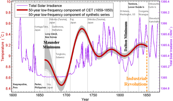
FIGURE 2.5 The low-frequency portion of the Central England temperature record, which could represent the Northern Hemisphere mean, is plotted along with the solar total solar irradiance (TSI) index and the occurrence of known large volcanic explosions. The figure indicates that the warming at the end of the Maunder Minimum around 1700 leads the increase in TSI by about 20-30 years and suggests that the warming may instead be a recovery from the cooling produced by the aerosols from a series of large volcanic eruptions between 1660 and 1680. SOURCE: Courtesy of K.K. Tung and J. Zhou, University of Washington, “Climate Response at Earth’s Surface to Cyclic and Secular Forcing,” presentation to the Workshop on the Effects of Solar Variability on Earth’s Climate, September 9, 2011.
MECHANISMS FOR SUN-CLIMATE CONNECTIONS
Mechanisms proposed to explain Earth’s climate response to solar variability can be grouped into three broad categories involving the response to variations in total solar irradiance, ultraviolet irradiance, and corpuscular radiation. The following talks at the workshop outlined the current rationale for considering how these stimuli might lead to significant responses by the climate system.
Issues in Climate Science Underlying Sun/Climate Research
Isaac M. Held, National Oceanic and Atmospheric Administration Geophysical Fluid Dynamics Laboratory
In his presentation Isaac Held asserted that the response of the climate to radiative heating—whether it comes from greenhouse gases trapping heat, stratospheric aerosols from volcanic eruptions or aerosols of various origin reflecting sunlight back to space, or finally variable TSI heating—involves both the troposphere and the ocean. The surface and the troposphere are intimately coupled through fast radiative-convective adjustments so that they respond as a whole, with part of the heat input going into the ocean. The ocean heat uptake and later slow release back to the atmosphere are the factors responsible for the difference between the transient response of the climate to radiative forcing as compared to the equilibrium climate (some 40-70 percent of the adjustment is achieved on a timescale on the order of 4 years, whereas equilibration takes centuries). This transient behavior can be demonstrated using a simple two-box model of the mixed layer and deep ocean, and it applies to all radiative forcings, such as to the Mount Pinatubo volcanic aerosols, as well as for the response to the 11-year solar cycle. On stratosphere-troposphere coupling, there is recent observational evidence that in the Southern Hemisphere the surface westerlies (and the storm track) have shifted poleward by a few degrees due possibly to the ozone hole over the South Pole in the stratosphere.
Held summarized work on this issue, focusing on a potential mechanism that employs the fact that cooling in the polar stratosphere associated with the loss of ozone increases the horizontal temperature gradient near the tropopause. Strengthening the horizontal temperature gradient alters in turn the fluxes of angular momentum by midlatitude eddies. The angular momentum budget of the troposphere controls the surface westerlies. This mechanism could work with volcanic aerosol warming or greenhouse gas cooling of the stratosphere, as well as for the solar warming of the lower stratosphere through ultraviolet absorption by ozone. Held noted that it is more difficult for perturbations to the middle stratosphere to engage this kind of mechanism. Other dynamics would be needed to communicate signals from the middle to the lower stratospheric regions capable of influencing Earth’s angular momentum budget significantly.
Indirect Climate Effects of the Sun Through Modulation of the Mean Circulation Structure
Caspar Ammann, National Center for Atmospheric Research
Caspar Amman emphasized the indirect climate effects of the Sun. He suggested that solar heating appears to be plausible as a radiative driver for the medieval warm period (approximately A.D. 900-1250) (Figure 2.6). When Earth’s radiative balance is altered, as in the case of a change in the solar-cycle forcing, not all locations are affected equally. He argued that although the global mean temperature change may be small, regional signatures in moisture, pressure, and temperature offer a consistent picture as revealed by proxy records. The equatorial central Pacific is generally colder, the runoff from rivers in Peru is reduced, and drier conditions affect the western United States. The western tropical Pacific is warmer, with a high-pressure system in the northwestern Pacific steering storm tracks further north, bringing moisture to Alaska and warming the interior of northern continents. The storm tracks drift to northern Europe, with moisture deposited in the northern part of Scandinavia although the Mediterranean
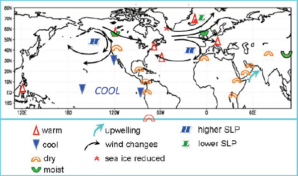
FIGURE 2.6 Dynamical mapping of persistent medieval anomalies in the Northern Hemisphere winter. SOURCE: N.E. Graham, C.M. Ammann, D. Fleitmann, K.M. Cobb, and J. Luterbacher, Support for global climate reorganization during the Medieval Climate Anomaly, Climate Dynamics 37:1217-1245, 2011.
remains dry. Global climate models (GCMs) currently do not reproduce the tropical features seen in proxy records, giving instead a more uniform warming. One model was able to present an improved spatial structure of response to medieval solar forcing when the solar flux into the Indian Ocean was artificially enhanced, producing a small expansion of the zonal overturning circulation of the atmosphere over the tropical Pacific Ocean (Walker cell) and inducing circumhemispheric circulations. The mechanisms involved are complex, and it is possible that both stratospheric-tropospheric dynamical coupling and coupled atmosphere-ocean dynamics are involved.
Climate Response to the Solar Cycle as Observed in the Stratosphere
Lon Hood, University of Arizona
Lon Hood’s presentation at the workshop covered the decadal signal in measurements of ozone mixing ratio in the upper stratosphere. These satellite measurements correlate with the ultraviolet variation associated with the 11-year solar cycle. The cyclic response of ozone in the middle stratosphere is rather weak, but larger again in the lower stratosphere. The WACCM3 climate model (which extends above the stratosphere) is able to simulate the upper- and middle-stratosphere signals but not the lower-stratosphere ones. Hood noted that it is possible that there is a change in the meridional circulation in the stratosphere, through the interaction with planetary waves, that could bring ozone from above to the lower stratosphere. The question is what could have produced the decadal variation in the planetary wave driving. There are both top-down and bottom-up potential mechanisms. The top-down (actually upper to lower stratosphere) mechanism involves the direct solar heating of the upper stratosphere, altering the circulation in such a way as to modify the planetary propagation. The bottom-up mechanism has the TSI radiative heating modifying the planetary wave amplitudes near the surface, which then propagate upward
into the stratosphere. The La Niña type of response during solar peak years proposed by Gerald Meehl and Harry van Loon could affect the production of planetary waves. However, Hood contended that regression analysis of sea surface temperature data does not show this pattern.
Solar Effects Transmitted by Stratosphere-Troposphere Coupling
Joanna D. Haigh, Imperial College, London
Joanna Haigh focused on the solar effects transmitted from the stratosphere to the troposphere through a dynamical coupling between the two layers. Solar-cycle signals in observational zonal mean temperature data show that when the Sun is more active, warming occurs in the tropical lower stratosphere and in vertical bands passing through the midlatitude troposphere (Figure 2.7). Consistent with this observation is an increase in the extent of the major meridional overturning (Hadley) cells of the tropical atmosphere and a slight shift toward the poles of the midlatitude jets. Surface air temperatures show a pattern in the North Atlantic consistent with the positive phase of the North Atlantic Oscillation. GCMs simulating solar influence with enhanced ultraviolet radiation show similar patterns of response, although the magnitude depends on the changes in solar spectrum (and implied influence on stratospheric ozone). Haigh claimed that studies with simpler models show that this pattern of response can be produced through the effects on wave momentum and heat fluxes of changing the thermal structure around the tropopause, and through a feedback on the mean state. She noted that recent measurements of the solar spectrum from the SORCE satellite imply large changes in ultraviolet that would reinforce these mechanisms.
Direct Solar Forcing of the Lower Atmosphere and Ocean
Gerald A. Meehl, National Center for Atmospheric Research
Gerald Meehl showed evidence that when observed sea surface temperature data are composited using only sunspot peak years, the tropical Pacific shows a pronounced La Niña-like pattern, with a cooling of almost 1°C in the equatorial eastern Pacific. This result has been seen in simulations using global coupled climate models. Diagnosis of the model results show that both bottom-up (related to air-sea coupling) and top-down (related to stratospheric ozone) mechanisms are needed to give the correct amplitude of the observed response (Figure 2.8). According to Meehl, the bottom-up mechanism involves greater solar heating of the tropical and subtropical ocean in the eastern Pacific for solar maximum, where there are relatively cloud-free conditions. The evaporated water vapor is transported to the western Pacific by the trade winds, enhancing the convection there and thereby increasing the strength of the Walker circulation. The enhanced surface easterlies drive a La Niña-like cold tongue in the eastern equatorial Pacific from the increased upwelling from the cold water below the thermocline. The signal appears in the sunspot peak years with dynamical coupled processes working on the timescale of El Niño-Southern Oscillation (ENSO), and those coupled dynamics then transition the tropical Pacific to a more El Niño-like pattern in the several years following the peak solar years. This La Niña-like pattern appears shortly after the rapid increase in solar activity from solar minimum to solar maximum, and is usually in evidence early in the broader solar maximum that lasts for several years. Thus, averaged over the several years of solar maximum, the initial La Niña-like pattern is not seen as strongly, and the El Niño-like pattern is more evident. The top-down mechanism related to stratospheric ozone also ends up strengthening tropical convection and precipitation, with the result that the same coupled air-sea dynamics produce responses similar to that for the bottom-up mechanism. Therefore, Meehl concluded, in the models the top-down and bottom-up mechanisms reinforce each other and work in the same sense to give measurable signals in sea surface temperature and precipitation in the tropics, with connections to midlatitude circulation (i.e., an anomalous high-pressure region in the North Pacific that extends to parts of North America).
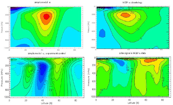
FIGURE 2.7 Northern hemisphere zonal and annual mean zonal wind (m/s) as a function of latitude and atmospheric pressure. Top row, right: climatology from National Centers for Environmental Prediction (NCEP) Reanalysis data set; left: climatology from a simplified climate model. Bottom row, right: solar 11-year-cycle signal from a multiple regression analysis of NCEP data; left: response in a simple model to heating applied (only) in the tropical lower stratosphere. Both sets of panels show a weakening and poleward shift in the westerly jet. This figure does not present a model simulation of solar effects but demonstrates that a thermal perturbation to the stratosphere can produce similar patterns in tropospheric response, giving indications as to potential mechanisms for a solar influence on climate. SOURCE: J. Haigh, M. Blackburn, and R. Day, The response of tropospheric circulation to perturbations in lower-stratospheric temperature, Journal of Climate 18:3672-3685, 2005; © Copyright 2005 American Meterological Society (AMS).
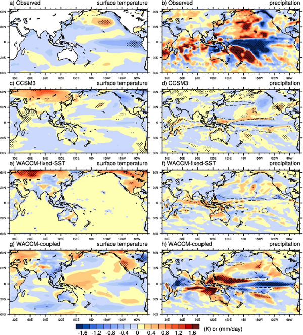
FIGURE 2.8 Composite averages for December-January-February for peak solar years (a,b). Observed, bottom-up coupled air-sea mechanism only (c,d); top-down stratospheric-ozone mechanism only (e,f); and both bottom-up and top-down mechanism (g,h). SOURCE: G.A. Meehl, J.M. Arblaster, K. Matthes, F. Sassi, and H. van Loon, Amplifying the Pacific climate system response to a small 11 year solar cycle forcing, Science 325:1114-1118, 2009; reprinted with permission from AAAS.
The Impact of Energetic Particle Precipitation on the Atmosphere
Charles Jackman, NASA Goddard Space Flight Center
Charles Jackman reported on solar energetic precipitating particles (EPPs), which are electrons and protons generated by solar flares, coronal mass ejections, and geomagnetic storms. They precipitate in Earth’s polar regions, where they enhance the production of HOx and NOx that destroy ozone in the mesosphere and upper stratosphere (Figure 2.9). Because of the relatively short lifetime of HOx constituents, most of the atmospheric and climate-relevant EPP focus is on NOx. Solar protons and electrons have episodic seasonal and solar cycle influence on the polar mesosphere. Measurements and models show that in years when significant winter-time meteorological events occur, EPP-enhanced NOx is transported from the upper mesosphere and lower thermosphere to lower altitudes where their impact may last several months, decreasing ozone by a few percent. There may even be a top-down effect where by EPP-NOx induced ozone destruction leads to changes in surface air temperature. Jackman noted that there may be a coupling between electron impact and climate,28,29 but that these findings need further work and affirmation. Jackman stated that GCRs (primarily protons and alpha particles) also create NOx and HOx but at lower altitudes due to their higher energy compared to solar particles. Because the incidence of GCRs varies inversely with solar activity, their effects on stratospheric chemistry tend to be out of phase with those of EPPs. Including GCRs in models results in an increase (relative to no GCRs) in NOy of 10-20 percent in the lower stratosphere, with the greatest effects at high latitudes, and a decrease is stratospheric ozone by around 1 percent. However, a GCR-driven solar-cycle variation in polar NOy is less than about 5 percent (greater at solar minimum than at solar maximum), resulting in annually averaged variations in polar ozone of less than 0.06 percent.
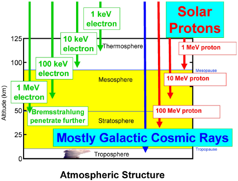
FIGURE 2.9 The atmospheric structure with incoming galactic cosmic rays and solar protons. SOURCE: C. Jackman, NASA Goddard Space Flight Center, “The Impact of Energetic Particle Precipitation on the Atmosphere,” presentation to the Workshop on the Effects of Solar Variability on Earth’s Climate, September 9, 2011.
_______________
28 E. Rozanov, L. Callis, M. Schlesinger, F. Yang, N. Andronova, and V. Zubov, Atmospheric response to NOy source due to energetic electron precipitation, Geophysical Research Letters 32:L14811, 2005.
29 A. Seppälä, C.E. Randall, M.A. Clilverd, E. Rozanov, and C.J. Rodger, Geomagnetic activity and polar surface air temperature variability, Journal of Geophysical Research 114:A10312, 2009.
Cosmic Rays and Cloud Nucleation
Jeffrey Pierce, Dalhousie University, Halifax, Nova Scotia
Evidence of a correlation between GCRs and climate via their influence on cloud cover has been debated, but insight into potential underlying physical mechanisms is providing a better understanding of the types of studies required to better quantify any impact. According to Jeffrey Pierce, there are two potential GCR-cloud-climate pathways:
1. GCRs enhance aerosol nucleation rates and cloud condensation nuclei concentrations through ionization of gases. These changes modify cloud formation, cloud amount, and subsequently, the shortwave radiation reaching the surface.
2. GCRs impact precipitation through the modification of near-cloud electrification with subsequent impact on the freezing of supercooled liquid droplets. Processes in this category could alter the global electrical circuit with potential but as yet unknown mechanisms.
Pierce noted that the first mechanism has been studied in far greater detail. International Satellite Cloud Climatology Project cloud analysis has suggested a 2 percent absolute change in cloud amount over the solar cycle, which corresponds to a 6 percent relative change.30 Although there is a 5-20 percent change in GCR-induced ionization in the troposphere over the solar cycle, this results (due to a number of dampening factors) in a smaller increase in nucleation rates, an even smaller increase in cloud condensation nuclei, and finally, a still smaller change in cloud amount. Thus it appears that the ion-aerosol clear-sky mechanism is too weak to explain the observed cloud changes, even with favorable assumptions for model inputs. Pierce asserted that a number of controlled experiments are necessary to better assess both the ion-aerosol hypothesis and the near-cloud hypothesis.31
_______________
30 K.S. Carslaw, R.G. Harrison, and J. Kirkby, Cosmic rays, clouds and climate, Science 298:1732-1737, 2002.
31 See also discussion by Daniel Baker, above.


