
D
Reports on Transportation Greenhouse Gas Emissions Projections to 2050
Many studies have examined the potential for greenhouse gas (GHG) emissions reductions in the U.S. transportation sector. Summarized below are the key studies that the National Research Council (NRC) Committee on Transitions to Alternative Vehicles and Fuels considered in its analysis. They include broad impact studies, such as the NRC report Real Prospects for Energy Efficiency in the United States (NRC, 2009b) and the Science article “Stabilization Wedges: Solving the Climate Problem for the Next 50 Years with Current Technologies” (Pacala and Socolow, 2004), as well as studies focused on specific components of the transportation sector, such as the Transportation Research Board (TRB) report Driving and the Built Environment: Effects of Compact Development on Motorized Travel, Energy Use, and CO2 Emissions. Special Report 298 (2009), which focuses on compact land use as a mitigation strategy. This summary is meant merely to serve as context for the committee’s charge—it does not attempt to review the validity of any findings contained herein. Any assertions made in the text of this appendix represent findings in the respective reports, not judgments of the current committee.
D.1 REAL PROSPECTS FOR ENERGY EFFICIENCY IN THE UNITED STATES (NRC, 2009b)
The NRC project “America’s Energy Future: Technology Opportunities, Risks, and Tradeoffs” evaluated current contributions and the likely future impacts, including estimated costs, of existing and new energy technologies. The study looked at three time frames: today through 2035, 2035 through 2050, and beyond 2050.
In its transportation analysis in the report Real Prospects for Energy Efficiency in the United States, the panel reviewed how current technologies are likely to improve and, as a result, be deployed. It then constructed two scenarios of vehicle and technology deployment as a means of estimating the potential overall effects of improved passenger vehicles and technologies on fuel consumption and GHG emissions.
For its analysis, the panel first assessed the likely technological changes expected over the three time frames and estimated the relative changes that might be seen among vehicle types. It then applied estimates of possible deployments of vehicle types to determine the overall potential reduction in petroleum use and GHG emissions that might be possible in the time frames of interest. The tables and figures below show the results. More details are available in the report itself and in the reports referenced in the text, especially Bandivadekar et al. (2008).
D.1.1 Relative Petroleum Use and Greenhouse-Gas Emissions by Vehicle Type
Table D.1 estimates the potential relative petroleum use and emissions of different vehicle types, both current and projected out to 2035. These estimates are based on studies that evaluated the fuel-consumption reduction potential of plausible improvements in vehicle technologies, including alternative powertrains. Each entry in Table D.1 is the fuel consumption (in gasoline equivalent) relative to that of the average vehicle in either the current or 2035 new-vehicle sales mix.
TABLE D.1 Potential Relative Vehicle Petroleum Use and Greenhouse Gas Emissions from Vehicle Efficiency Improvements
| Propulsion System | Petroleum Consumption (gasoline eq.) |
Greenhouse Gas Emissionsa | |||||||
| Relative to 2005 gasoline ICE | Relative to 2035 gasoline ICE | Relative to current gasoline ICE | Relative to 2035 gasoline ICE | ||||||
| 2005 gasoline HEV | 1.00 | — | 1.00 | — | |||||
| 2005 turbocharged gasoline | 0.90 | — | 0.90 | — | |||||
| 2005 diesel | 0.80 | — | 0.80 | — | |||||
| 2005 hybrid electric vehicle (HEV) | 0.75 | — | 0.75 | — | |||||
| 2035 gasoline | 0.65 | 1.00 | 0.65 | 1.00 | |||||
| 2035 turbocharged gasoline | 0.60 | 0.90 | 0.60 | 0.90 | |||||
| 2035 diesel | 0.55 | 0.85 | 0.55 | 0.85 | |||||
| 2035 HEV | 0.40 | 0.60 | 0.40 | 0.60 | |||||
| 2035 plug-in hybrid (PHEV) | 0.20 | 0.30 | 0.35-0.45 | 0.55-0.70 | |||||
| 2035 battery electric vehicle (BEV) | None | 0.35-0.50 | 0.55-0.80 | ||||||
| 2035 hydrogen fuel cell vehicle (HFCV) | None | 0.30-0.40 | 0.45-0.60 | ||||||
NOTE: These estimates assume that vehicle performance (maximum acceleration and power-to-weight ratio) and size remain the same as today’s average new-vehicle values. That is, the improvements in propulsion efficiency are used solely to decrease fuel consumption rather than to offset increases in vehicle performance and size. Estimates have been rounded to the nearest 0.05. BEVs and HFCVs are expected to have shorter driving ranges than PHEVs between rechargings or refuelings.
a Greenhouse gas emissions from the electricity used in 2035 PHEVs, 2035 BHEVs, and 2035 HFCVs are estimated from the projected U.S. average electricity grid mix in 2035 (Kromer and Heywood, 2008). Greenhouse gas emissions from hydrogen production are estimated for hydrogen produced from natural gas.
SOURCE: Bandivadekar et al. (2008). Estimates based on assessments by An and Santini (2004); Wohlecker et al. (2007); Cheah et al. (2007); NPC (2007); and NRC (2004).
These values assume fleet performance and interior size are essentially the same as those of vehicles coming out on the market today, although the load is reduced via lightweighting (20 percent weight reduction), aerodynamics (25 percent reduction in vehicle drag), and rolling resistance (33 percent reduction in tire rolling-friction coefficient). The values in the table are meant to represent what could be achieved, not what is likely to be achieved.
D.1.2 Incremental Purchase Cost by Vehicle Type
These fuel economy improvements are obtained at a premium. Table D.2 depicts the estimated increase in vehicle cost (compared to today’s car and truck average prices for a new vehicle). These cost estimates are based on a number of studies examining current and future vehicle technology costs for manufacturers. An additional 40 percent mark-up is assumed to account for indirect costs, reflecting with the 1.4 retail price equivalent what a consumer would actually pay for the vehicle. However, different manufacturers may choose to subsidize particular technologies with different deployment strategies in mind, so these costs are subject to large uncertainty.
TABLE D.2 Estimated Additional Cost to Purchaser of Advanced Vehicles Relative to Baseline 2005 Average Gasoline Vehicles
| Additional Retail Price (2007 dollars) | ||
| Propulsion System | Car | Light Truck |
| 2005 gasoline ICEV | 0 | 0 |
| 2005 diesel ICEV | 1,700 | 2,100 |
| 2005 hybrid HEV | 4,900 | 6,300 |
| 2035 gasoline ICEV | 2,000 | 2,400 |
| 2035 diesel ICEV | 3,600 | 4,500 |
| 2035 hybrid HEV | 4,500 | 5,500 |
| 2035 PHEV | 7,800 | 10,500 |
| 2035 BEV | 16,000 | 24,000 |
| 2035 HFCV | 7,300 | 10,000 |
NOTE: Costs listed are additional costs only, relative to baseline average new car and light truck purchase prices (in 2007 dollars) that were calculated as follows:
• Average new car: $14,000 production cost × 1.4 retail price equivalent = an average purchase price of $19,600; and
• Average new light truck: $15,000 × 1.4 = $21,000. For the purpose of these estimates, the PHEV all-electric driving range is 30 miles; the BEV driving range is 200 miles. Advanced battery and fuel-cell system prices are based on target battery and fuel-cell costs.
SOURCE: Bandivadekar et al. (2008).
D.1.3 Deployment
Because these alternative powertrains are at an emerging stage of deployment, it is difficult to ascertain what the vehicle mix will look like in the future. For example, while the NRC report Transitions to Alternative Transport Technologies: A Focus on Hydrogen (NRC, 2008) concluded that up to 2 million hydrogen fuel cell vehicles (HFCVs) could be on the road by 2020, it is unlikely that such a rapid transformation would take place, given the infrastructural needs of a hydrogen-powered fleet.
Table D.3 is an attempt by the Committee on America’s Energy Future to project what the likely future vehicle fleet mix could look like, focusing in particular on alternative powertrains. These numbers are for new sales only and do not represent the total fleet mix. The committee did not foresee significant deployment of plug-in hybrid electric vehicles (PHEVs), battery-powered electric vehicles (BEVs), or HFCVs without significant technical progress resulting in significant cost reduction below the levels indicated in Table D.2.
Table D.4 depicts how consumption would change given such a potential vehicle mix. The committee suggested that in the future, some of the reduction in fuel consumption for a fleet comprised of vehicles equivalent to today will be offset by changes in the fleet (increased vehicle performance, size, and weight). There are two scenarios—the first (optimistic) would meet the Corporate Average Fuel Economy (CAFE) standards outlined in Energy Independence and Security Act of 2007 (EISA 2007) (35 mpg by 2020), as required; the second (conservative) would see those standards delayed by 5 years and put less of an emphasis on fuel economy. Neither scenario considered BEVs or HFCVs. In both scenarios, advanced powertrains are imagined to make up more than half of the new vehicle fleet in 2035, resulting in the optimistic case of a 100 percent increase in fuel efficiency up to 50 mpg. For reference, the most recent proposed rule for the 2017-2025 model years (MYs) by the Environmental Protection Agency and the National Highway Traffic Safety Administration has a CAFE standard of 40.9 mpg by MY2021 with a conditional second phase leading to a 49.6 mpg fleet-wide average by MY2025.
TABLE D.3 Plausible Share of Advance Light-Duty Vehicles in the New-Vehicle Market by 2020 and 2035 (%)
| Propulsion System | 2020 | 2035 |
| Turbocharged gasoline SI vehicles | 10-15 | 25-35 |
| Diesel vehicles | 6-12 | 10-20 |
| Gasoline hybrid vehicles | 10-15 | 15-40 |
| PHEV | 1-3 | 7-15 |
| HFCV | 0-1 | 3-6 |
| BEV | 0-2 | 3-10 |
NOTE: The percentage of hydrogen fuel-cell vehicles considered “plausible” is in contrast to the percentages reported in Transitions to Alternative Transport Technologies: A Focus on Hydrogen (NRC, 2008), which represent “maximum practical” shares.
TABLE D.4 Illustrative Vehicle Sales Mix Scenarios
| Market Share by Power Train (percent) | ||||||||||
| % Emphasis on Reducing Fuel Consumptiona | % Light Trucks vs. Cars | % Vehicle Weight Reduction | Naturally Aspirated SI | Turbo SI | Diesel | Hybrid | Plug-in Hybrid | Total Advanced Power Train | % Fuel Efficiency Increase from Today | |
| Optimisticb | ||||||||||
| 2020 | 75 | 40 | 17 | 52 | 26 | 7 | 15 | 0 | 48 | +38 |
| 2035 | 75 | 30 | 25 | 36 | 26 | 9 | 20 | 9 | 64 | +100 |
| Conservativec | ||||||||||
| 2025 | 50 | 40 | 17 | 55 | 24 | 7 | 14 | 0 | 45 | +38 |
| 2035 | 50 | 40 | 20 | 49 | 21 | 7 | 16 | 7 | 51 | +62 |
a The amount of the efficiency improvement that is dedicated to reducing fuel consumption (i.e., that is not offset by increases in vehicles power, size, and weight).
b The optimistic scenario meets the new CAFE target of 35 mpg in 2020, and then extrapolates this rate of improvement through 2035. In this case, the average fuel economy in 2035 reaches 52 mpg, roughly double today’s value.
c The conservative scenario achieves the new CAFE target of 35 mpg only in 2025 (5 years later) and extrapolates this rate of improvement through 2035, when the average fuel economy reaches only 60 percent above today’s value.
D.1.4 Cumulative Effects
Figure D.1 shows, for the conservative and optimistic scenarios, the corresponding annual gasoline consumption of the United States in-use light-duty vehicle (LDV) fleet from the present out to 2035. A no-change baseline assumes that all of the efficiency improvements go to vehicles size, weight, and power, as has occurred since 1982. The cumulative fuel savings under each scenario compared with this no-change baseline are indicated. Note that this no-change baseline includes some growth in overall fleet size and miles driven but no resulting change in vehicle fuel economy. No similar assessment is given for GHG emissions.
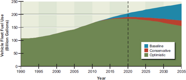
FIGURE D.1 Fuel use for the U.S. in-use light-duty vehicle fleet out to 2035.
SOURCE: Cheah and Heywood (2008).
D.2 LIQUID TRANSPORTATION FUELS FROM COAL AND BIOMASS—TECHNOLOGICAL STATUS, COSTS, AND ENVIRONMENTAL IMPACTS (NRC, 2009a)
The NRC committee examining America’s energy future also looked into developments in the fuels sector related to conversion from coal and biomass. Below are the study’s main findings as it pertains to the automotive sector.
Figure D.2 shows the estimated gasoline-equivalent costs of alternative liquid fuels produced from coal, biomass, or a combination of the two. The fuels would be produced by either biochemical conversion to ethanol, thermochemical conversion via Fischer-Tropsch, or thermochemical conversion via the methanol-to-gasoline process. Carbon capture and storage (CCS) could be used in either thermochemical conversion process to reduce GHG emissions, so the costs are shown both with and without CCS. Also shown for comparison are the prices for gasoline based on two different crude oil prices, (2007) $60 or (2007) $100 per barrel. At $60 per barrel, only the coal-to-liquid fuels are comparably priced. Even at $100 per barrel, biomass-to-liquid fuels are not cost competitive without carbon pricing.
Carbon pricing has a significant effect on competitiveness. The committee examined the costs with a carbon price of $50 per tonne (1,000 kg) CO2-equivalent, and biomass-to-liquid fuels become cost competitive with standard gasoline at $100 per barrel crude oil. If CCS is added to the biomass-to-liquid plant, it becomes cost competitive by $80 per barrel crude oil, as does cellulosic ethanol.
The reason for this shift in competitiveness can be seen in Table D.5. Here is tabulated the committee’s values for lifecycle emissions for the various fuels. Fuels generated from biomass have a net-negative emissions of CO2 over the lifecycle of the fuel, where the lifecycle is defined from the harvesting of the fuel to its consumption.
In addition to examining the costs and benefits associated with alternative fuels, the committee studied its potential for deployment. Figure D.3 depicts the maximum potential build-up of cellulosic ethanol, one of the alternative fuels specified as part of the Renewable Fuel Standard 2 (RFS2). Two scenarios are shown in Figure D.3—the first (in blue) is the maximum build-up if it is assumed to be similar to that of grain ethanol; the second (in red) is a more aggressive scenario leading to approximately double the capacity of grain ethanol. Neither scenario is meant to be a prediction but a limit.
The build-up of cellulosic-ethanol is, like other biomass fuels, highly dependent on the prices of other fuels. However, if cellulosic-ethanol plants are shown to be commercially viable, cellulosic
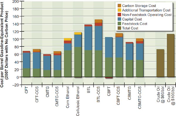
FIGURE D.2 Costs of alternative liquid fuels produced from coal and biomass assuming no carbon price. BTL = biomass-to-liquid fuel; CBFT = coal-and-biomass-to-liquid fuel, Fischer-Tropsch; CBMTG = coal-and-biomass-to-liquid fuel, methanol-to-gasoline; CCS = carbon capture and storage; CFT = coal-to-liquid fuel, Fischer-Tropsch; CMTG = coal-to-liquid fuel, methanol-to-gasoline.
TABLE D.5 Net CO2 Emissions
(tonnes per barrel gasoline eqivalent)
| Fuel Type | Net CO2 |
| CFT | 1.06 |
| CFT-CCS | 0.44 |
| CMTG | 1.10 |
| CMTG-CCS | 0.42 |
| Corn ethanol | 0.37 |
| Cellulosic ethanol | –0.10 |
| BTL | –0.13 |
| BTL-CCS | –0.76 |
| CBFT | 0.49 |
| CBFT-CCS | –0.21 |
| CBMTG | 0.47 |
| CBMTG-CCS | –0.13 |
| Gasoline | 0.42 |
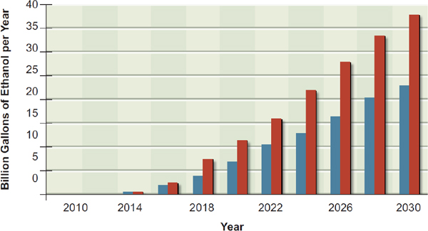
FIGURE D.3 Cellulosic-ethanol capacity-building scenarios starting with commercial demonstration plants in 2009 with first commercial-scale plants following thereafter, building to 1 billion gallons of cellulosic ethanol per year in 2015. Capacity-building beyond 2015 is in accordance with the maximum capacity build achieved for grain ethanol (blue bars) and a more aggressive capacity build of about twice that achieved for grain ethanol (red bars). The maximum build rate could achieve the 2022 RFS2 mandate of 16 billion gallons of cellulosic ethanol per year, but it would be a stretch.
ethanol could replace up to 0.5 million barrels of gasoline equivalent per day by 2020 and 1.7 million barrels per day by 2035. The necessary supply of tons of biomass per year of 440 million dry tons in 2035 would be only marginally larger than the estimated annual supply of 400 million dry tons of cellulosic biomass that could be produced sustainably with technologies and management practices available in 2008 and well short of the estimated 550 million dry tons that would be deliverable by 2020.
D.3 TRANSPORTATION’S ROLE IN REDUCING U.S. GREENHOUSE GAS EMISSIONS (DOT, 2010)
Under EISA 2007, the Department of Transportation (DOT) was required to report on the potential strategies for reducing GHG emissions within the transportation sector. Select results from this two-volume report are summarized below.
D.3.1 Alternative Fuels
Because this report was written during the rulemaking for the second generation of the Renewable Fuel Standard (RFS2), biofuels were excluded from analysis. However, numerous other alternatives to gasoline and diesel were given, including compressed natural gas (CNG), hydrogen, and electricity. The GHG emissions reductions for each of these fuels is summarized in Table D.6. Values for electricity as a “fuel” are calculated for BEVs with all-electric ranges of 100 and 200 miles. Fuel
TABLE D.6 Costs and Benefits for Alternative Fuels Out to 2030 to 2050
| Fuel | Year | Incremental Vehicle Cost | Discounted Fuel Cost ($) | Net Discounted Cost/Savings | Average GHG Reduction (Tonnes/yr.) | Net Dollars per Tonne per Year | |||
| Compressed natural gas | 2030 | $3,000 | −$4,460 | −$1,460 | 0.7 | −$132 to −$50 | |||
| Hydrogen | 2020 | $10,000 | −$3,500 to $4,400 | $6,500 to $14,400 | 2.7 | $151 to $333 | |||
| 2030 to 2050 | $1,500 to $5,300 | −$11,900 to −$8,300 | −$10,300 to −$3,000 | 3.3 | −$199 to −$57 | ||||
| BEV100 | 2030 | $6,000 | −$11,300 | −$3,500 | 3.1 to 3.7 | −$90 to −$106 | |||
| BEV200 | 2030 | $10,200 | −$11,300 | −$1,100 | 3.1 to 3.7 | −$19 to −$22 | |||
generated from fossil fuel products such as liquid propane, Fischer-Tropsch gas-to-diesel, and coal-to-liquid gasoline were also discussed but found to be too carbon intensive to be used to effect significant GHG reductions; in fact, in one cited example, an sport-utility vehicle (SUV) fueled with gasoline derived from coal released twice as much GHG emissions per mile compared to conventional fuel when you look at the entire fuel lifecycle. CCS would help eliminate some of the upstream GHG emissions, but the DOT study viewed this as still in the research and development (R&D) stage and did not include such features in its report.
A crucial question for the application of non-traditional fuels is the ability for vehicles using those fuels to penetrate the marketplace. In the case of natural gas, this report estimates that approximately 19 million vehicles could be fueled by CNG without significantly affecting the price and supply of domestic natural gas; furthermore, they cite an established infrastructure and current vehicle fleet as evidence of its potential for scalability. For hydrogen, because there is no established model for the vehicles or infrastructure, the estimates ranged from 93,000 by 2030 to 2 million vehicles on the road by 2025 at a cost of approximately $10 billion. Finally, electric vehicles were estimated to be as much as 9 percent of new vehicle sales in 2030, or approximately 10 million total vehicles on the road; however, this value is noted as highly speculative.
D.3.2 Vehicle Technologies
There were four main strategies considered to reduce GHG emissions from gasoline-powered LDVs, (1) advanced conventional gasoline engine technologies, (2) conversion to diesel, (3) hybrid electric vehicles (HEVs), and (4) PHEVs. The resultant GHG reductions and costs are shown in Table D.7. Hydrogen fuel cells were considered separately because they would require a transition to an alternative fuel.
In addition to technology that addresses fuel consumption, it is possible to reduce GHG emissions by addressing mobile air conditioning (MAC) systems. Current, MAC systems contribute approximately 3.5 percent of all LDV GHG emission. There are three approaches to reducing emissions associated with the operation of the MAC system: (1) reduce the leakage of the refrigerant to the atmosphere; (2) reduce the greenhouse warming potential of the refrigerant itself; and (3) reduce the engine load associated with running the air conditioning system. Alternative refrigerants would result in reductions of 91.3 to 99.9 percent. Reductions in engine load could reduce GHG emissions from MAC operation by as much as 30 percent.
TABLE D.7 Greenhouse Gas Reductions and Costs for the Implementation of Different Fuel Economy Technologies
| Technology | Year | Conventional Vehicle MPGGE | Scenario MPG | GHG Emission Reduction Range | Average Incremental Vehicle Cost | ||||
| Min. | Max. | Min. | Max. | Min. | Max. | ||||
| Advanced ICE | 2010 | 21.9 | 26.7 | 29.3 | 18% | 25% | −$60 | $2,399 | |
| 2030+ | 28.2 | 30.8 | 40.4 | 8% | 30% | ||||
| Advanced diesel | 2010 | 21.8 | 27.6 | 31.2 | 21% | 29% | $1,567 | $5,617 | |
| 2030+ | 28.2 | 28.2 | 33.2 | 0% | 16% | ||||
| Hybrid electric vehicles | 2010 | 21.8 | 26.2 | 53.9 | 17% | 60% | $3,700 | $5,700 | |
| 2030+ | 28.2 | 38.3 | 60.8 | 26% | 54% | $2,300 | $4,100 | ||
| PHEV-10 | 2030 | 28.2 | 36% | 60% | $3,100 | ||||
| 2050 | 38% | 62% | $2,900 | ||||||
| PHEV-40 | 2030 | 28.2 | 51% | 70% | $6,100 | ||||
| 2050 | 57% | 74% | $5,300 | ||||||
| PHEV-60 | 2030 | 28.2 | 58% | 74% | $8,100 | ||||
| 2050 | 65% | 74% | $6,900 | ||||||
NOTE: PHEV values recalculated using the range of hybrid electric vehicle reductions from the table above instead of the nominal 40 percent used in the text. Utility factors for the PHEV-10, -40, and -60 are 0.23, 0.60, and 0.75, respectively.
D.3.3 Vehicle Miles Traveled Strategies
An alternative way to reduce fuel consumption by the transportation sector is to simply use vehicles less. There are numerous ways of reducing vehicle miles traveled (VMT)—among them are telecommuting, increased use of public transportation, compact land use, traffic management, and eco-driving. Implementing all of these potential strategies could result in a net GHG reduction of 12 to 30 percent by 2030 and 14 to 37 percent by 2050,1 with the largest contribution coming from compact land use (2.5 to 7.8 percent in 2030 and 5.0 to 16 percent in 2050). Details of the strategies to improve system efficiency and reduce carbon-intensive travel activities can be found in DOT (2010) in Tables 3.5 and 3.6, respectively.
D.4 SUSTAINABLE TRANSPORTATION ENERGY PATHWAYS (UCD, 2011)
The Institute for Transportation Studies (ITS) at the University of California, Davis, compiled its research on sustainable transportation pathways from 2007-2010. Its work focused on six main technology pathways moving forward: biofuels; advanced, efficient internal combustion engines (ICEs); HEVs; PHEVs; BEVs; and HFCVs. The report looked at the costs of these technologies, the challenges facing implementation of these technologies, their ability to reduce GHG emissions, and policy options that could be used to push these technologies into the mainstream in order to reduce GHG emissions.
_____________________________
1 Tables 3.5 and 3.6 in Volume 1 show the cost effectiveness of GHG emission reductions by reducing VMT of the light-duty vehicle fleet by 2030. Combined reductions are treated as multiplicative so as to not overcount.
D.4.1 Technology Costs
The ITS researchers calculated costs for each advanced vehicle technology in 2030 and compared them to a 2007 baseline, port-injected gasoline vehicle (27.1 mpg). They found that advanced ICE technology offers an extremely cost-effective path to obtain a 43 percent reduction in fuel consumption, with a break-even fuel price of $3.62/gallon.2 They looked at a range of battery and hydrogen fuel cell prices to examine the potential for novel technologies to make a significant impact. Although hybrid vehicles require a small battery, it is a small component of the cost of the vehicle, and because of its 33 percent reduction in consumption beyond that of the advanced ICE vehicle (ICEV), the advanced hybrid vehicle has a break-even cost of $2.29-$2.61/gallon. According to the ITS analysis, the PHEV-40 offers the greatest potential for energy savings at 79 percent; however, at $500/kWh the break-even cost is $5.29, and it does not slip below $4 unless the battery price comes down to $300/kWh. HFCVs offer a similar fuel benefit, but because of the additional cost of hydrogen as a fuel source, the break-even cost is $4.02/gallon for a $50/kW fuel cell and $2.86/gallon if the $30/kW fuel cell target set by the Department of Energy (DOE) is met. According to the ITS report, BEVs would require $5/gallon gasoline to break even, even for a battery at $300/kWh, due to the extremely high costs of the lithium-ion (Li-ion) battery.
D.4.2 Requirements for Deployment
In order to understand the barriers facing a transition to any of the advanced fuels (hydrogen, electricity, biofuels), the ITS researchers examined the capability of fueling 10 percent of the LDV fleet with these fuels.
D.4.2.1 Hydrogen
Supporting 10 percent of the LDV fleet would require approximately 250,000 kg of platinum (Pt), more than the current world annual production. It is likely, therefore, that platinum recycling would be necessary and add to the cost of hydrogen deployment. Additionally, because the initial deployment of hydrogen as a fuel is almost certainly going to be derived from natural gas, about 3 percent of the total natural gas in use today would be needed to generate the required 5 billion kg of hydrogen. Most of the hydrogen is expected to be reformed on site, although approximately 9,000 miles of pipeline centered in urban areas would be required. The investment necessary to support such a fleet size would be $38 billion: $21 billion would be used for the 14,000 onsite reformers, $4 billion for biomass plants with CCS, $9 billion for pipeline, and $4 billion for pipeline stations.
D.4.2.2 Electricity
For a 10 percent fraction of the country’s LDVs, approximately 28 GW of night-time energy would be necessary, or less than 5 percent of the U.S. generation capacity. Over the course of the next 40 years, it is also expected that the grid will become become greener. While major system upgrades are unlikely to be necessary, there may be a need for local “smart grid” interfaces. The largest deployment cost is going to in home chargers, which are estimated at $800-$2,100 per installation. Summed over 10 percent of the total LDV fleet, this would require an investment of $16 billion to $42 billion. There may be additional infrastructure required for fast charging at waypoints.
_____________________________
2 Break-even gas prices are calculated based on a 5-year return with a 4 percent discount rate and an average VMT of 12,000 miles per year.
D.4.2.3 Biofuels
To fully fuel 10 percent of the LDV fleet with biofuels would require about 12 billion gallons of gasoline equivalent per year. This, in turn, would be derived primarily from corn (requiring ~30 percent of the current annual supply) and forest, agricultural, and municipal wastes. To distribute the biofuels, an additional 7,000 rail tank cars would be required. If the fuels produced are drop-in fuels, no additional infrastructure is required for fueling; however, if it is entirely ethanol, 20,000 E85 stations would be required to support 20 million vehicles. $50 billion to $70 billion would be required in total, with 80 percent of that for biorefineries (150 corn ethanol plants, 76 cellulosic biorefineries, and/or 16 biodiesel plants) and the remainder to support the biofuel delivery system.
D.4.3 Scenarios to Reduce Greenhouse Gas Emissions
Looking forward to 2050, the researchers at ITS came up with three types of future scenarios: (1) the business-as-usual (BAU) scenario; (2) “silver bullet” scenarios, where an individual technology is deployed as aggressively as possible; and (3) “deep-reduction” scenarios, where a combination of technologies are deployed in tandem to maximize the reductions in GHGs.
D.4.3.1 Reference Scenario
The reference scenario is dependent on a 69 percent population increase, significant increase (102 percent) in per-capita transport demand (mostly due to an expansion of air-based travel), and moderate efficiency improvement (45 percent, or about 1 percent each year). In the LDV fleet, these efficiency improvements would result in a fleetwide fuel economy of 35 mpg by 2050. The carbon intensity of the grid remains essential the same as 1990 levels, owing to the presumed continued dominance of carbon-based fuels. Any improvements in carbon intensity from the increased blending of biofuels into gasoline is offset by the increased usage of unconventional fossil fuel sources such as oil sands. In this scenario, domestic GHG emissions from the transportation would increase by 82 percent.
D.4.3.2 Silver Bullet Scenarios
The available technologies have been described in USD (2010). Figure D.4 depicts the GHG emissions with full deployment of each technology. It is clear that no single technology can meet even the 50 percent reduction in GHG emissions from 1990—in fact, only one (a 50 percent reduction in average VMT across the transportation sector, with an increased use of mass transit and high-density land use) even breaks even with 1990 levels. In the hydrogen-intensive scenario, low-carbon hydrogen production (24.3 gCO2e/MJ) is assumed, and HFCVs make up 60 percent of the fleet. In the electricity-intensive scenario, the carbon intensity of the grid is assumed to be reduced by 79 percent below 1990 values, and the fleet is presumed to be composed of half BEVs and half PHEVs in 2050.
D.4.3.3 Deep-Reduction Scenarios
The study focused on three deep-reduction scenarios: (1) U.S. Efficient Biofuels 50in50, which looks at a deep penetration of biofuels and improved efficiency; (2) U.S. Electric Drive 50in50, which focuses on widespread adoption of BEVs, PHEVs, and HFCVs; and (3) U.S. Multi-Strategy 80in50, which effectively combines the two 50in50 plans. Assumptions of the three plans are shown in Table D.8,
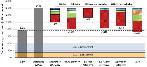
FIGURE D.4 Greenhouse gas (GHG) emissions for the transportation sector in 2050 for scenarios with the widespread implementation of various GHG-reducing strategies. 1990 levels and the BAU reference case are shown for comparison. SOURCE: McCollum and Yang (2009).
and the results for the three scenarios are shown in Figure D.5. In outlining these deep-reduction scenarios, there are implicit changes in fuel generation as well such as a cleaner grid and low-carbon-intensity hydrogen production in order to achieve the results depicted in Figure D.5.
All scenarios involve a significant reduction in VMT. Somewhat counterintuitively, increased vehicle efficiency (due to the efficiency of electric motors and hydrogen-powered engines) in the Electric Drive scenario actually reduces fuel usage beyond the Efficient Biofuel scenario. In all cases, biofuels are used to reduce emissions from the expected increase in air travel; however, concerns about the availability of feedstock does raise uncertainty in its application. In fact, the Multi-Strategy 80in50 scenario would require 1.8 billion dry tons of biomass to produce both hydrogen (with CCS) for LDVs and the biofuels necessary to replace all aviation fuel. For shifting a large fraction of fuel to the electrical grid, an increasing diversity of natural resources (wind, solar) is more than adequate.
D.4.4 Policy Options for GHG Emissions
Policy will likely play a major role in enacting any of the transformative scenarios described in the previous section. In particular, ITS examined how cap-and-trade both economywide and in the transportation sector can play a role in driving these scenarios. They also explored the potential ramifications of a biofuel mandate and, conversely, a lack of cellulosic biofuels.
The results of the ITS study are shown in Figure D.6. The scenarios studied include a CO2 emission cap of 10 percent, 20 percent, and 30 percent in both transportation and economywide; a 30 percent economywide and transportation cap without a complementary biofuel mandate and/or without access to biofuels; and a 40 percent and 50 percent economywide cap on CO2 emissions. A major result in all studies is the complete lack of hydrogen vehicle penetration—the authors note, however, that hydrogen penetration is particularly sensitive to the cost of fuel cell technology, oil price, and discount rate assumed. By comparing the scenarios with and without a biofuel mandate, it is clear that ethanol use in the fleet for flex-fuel vehicles is driven by a mandate; however, looking at the fuel mix results, ethanol still can have significant penetration, even without a mandate. It can also be shown that biofuels are not a
necessary component of meeting an emissions cap, although without biofuels available, cumulative fuel usage must decrease substantially compared to other scenarios, requiring significantly more efficient vehicles. In all scenarios, whether or not the transportation sector is specifically capped, the largest reduction in CO2 emissions comes from a greening of the electric grid.
TABLE D.8 Assumptions for the Three Deep-Reduction Scenarios for U.S. Domestic Emissions in 2050
| Shares of Miles by Fuel Type | Normalized Transport Intensity (1990=100%) | Normalized Energy Intensity (1990=100%) | Normalized Carbon Intensity (1990=100%) | ||||||
| Petroleum | Biofuels | Hydrogen | Electricity | ||||||
| U.S.-Efficient Biofuels 50 in 50 | |||||||||
| LDV | 0 | 100 | 0 | 0 | 137 | 33 | 13 | ||
| HDV | 80 | 20 | 0 | 0 | 149 | 52 | 82 | ||
| Aviation | 100 | 0 | 0 | 0 | 234 | 36 | 100 | ||
| Rail | 84 | 0 | 0 | 16 | 171 | 59 | 80 | ||
| Marine/Ag/off-road | 100 | 0 | 0 | 0 | 117 | 40 | 101 | ||
| All subsectors combined | 35 | 64 | 0 | 1 | 152 | 37 | 53 | ||
| Fuel demand (billion GGE) | 77.2 | 88.5 | 0.0 | 1.3 | |||||
| Carbon intensity (gCO2e/MJ) | 90-96 | 12.3 | - | 44 | |||||
| U.S.-Electric Drive 50 in 50 | |||||||||
| LDV | 10 | 0 | 60 | 30 | 137 | 24 | 40 | ||
| HDV | 72 | 0 | 22 | 5 | 149 | 60 | 100 | ||
| Aviation | 20 | 75 | 5 | 0 | 234 | 37 | 32 | ||
| Rail | 0 | 0 | 0 | 100 | 171 | 38 | 43 | ||
| Marine/Ag/off-road | 62 | 0 | 38 | 0 | 117 | 40 | 78 | ||
| All subsectors combined | 17 | 17 | 42 | 24 | 152 | 33 | 59 | ||
| Fuel demand (billion GGE) | 64.6 | 21.2 | 42.2 | 19.7 | |||||
| Carbon intensity (gCO2e/MJ) | 90-96 | 12.3 | 24 | 44 | |||||
| U.S.-Multi-Strategy 80 in 50 | |||||||||
| LDV | 0 | 10 | 60 | 30 | 137 | 22 | 30 | ||
| HDV | 0 | 63 | 28 | 9 | 149 | 58 | 19 | ||
| Aviation | 0 | 100 | 0 | 0 | 234 | 37 | 14 | ||
| Rail | 0 | 0 | 0 | 100 | 171 | 38 | 43 | ||
| Marine/Ag/off-road | 2 | 79 | 20 | 0 | 117 | 40 | 28 | ||
| All subsectors combined | 0 | 36 | 40 | 24 | 152 | 32 | 24 | ||
| Fuel demand (billion GGE) | 1.9 | 82.3 | 39.3 | 19.1 | |||||
| Carbon intensity (gCO2e/MJ) | 90-96 | 12.3 | 24 | 44 | |||||
NOTE: Shown are the transport, energy, and carbon intensities as well as the share of transport miles for each fuel type/technology.
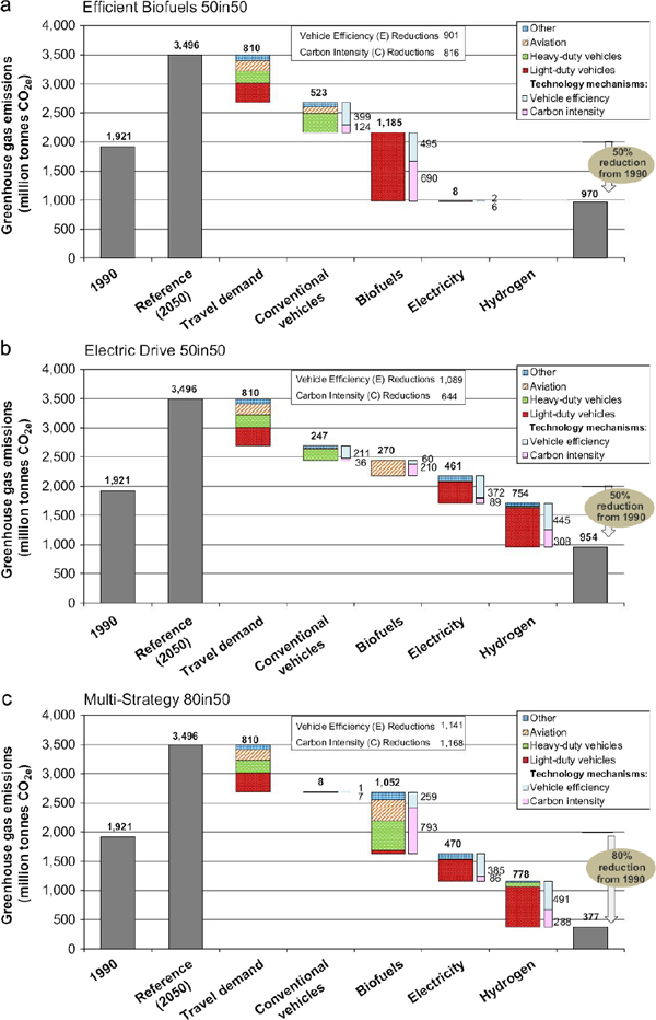
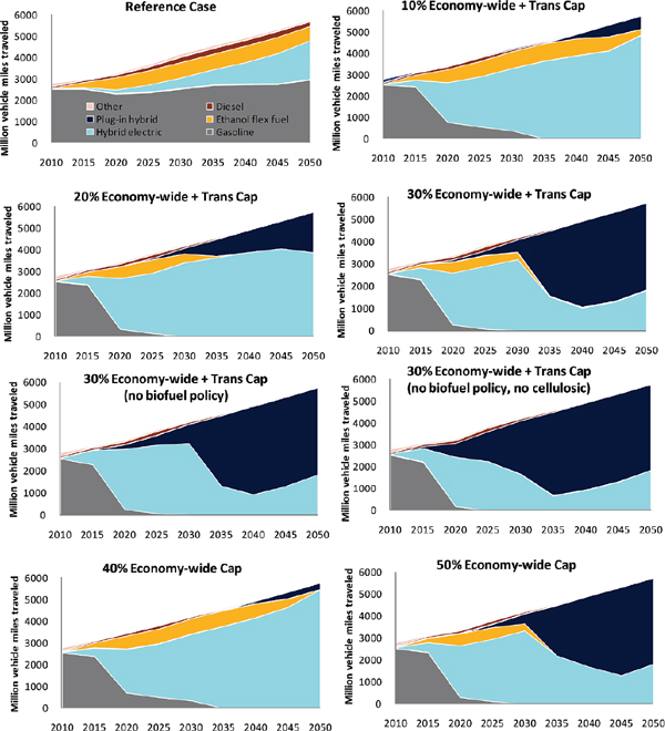
FIGURE D.6 Vehicle miles traveled for various vehicle technologies over time under different cap-and-trade scenarios.
D.5 LIMITING THE MAGNITUDE OF FUTURE CLIMATE CHANGE (NRC, 2010a)
The America’s Climate Choices Panel on Limiting the Magnitude of Climate Change was charged to describe, analyze, and assess strategies for reducing the net future human influence on climate, including both technology and policy options. The panel’s report focuses on actions to reduce domestic GHG emissions and other human drivers of climate change, such as changes in land use. As part of its analysis, it examined the energy demand from the transportation sector.
Shifting to low-carbon fuels provides one path to a reduction of GHG emissions. While there are vehicle technologies available that are already in use and could be rapidly deployed over the next decade (e.g., cylinder deactivation and direct injection), alternative-powertrain vehicles (PHEVs, HFCVs, BEVs) could provide a more significant reduction in GHG emissions by shifting away from gasoline as a primary fuel. However, in the case of electric vehicles, shifting the fuel source to the grid would require a decarbonization of the grid to make a significant impact. New natural gas plants can compete with new coal plants thanks to the plummeting costs of natural gas, and it emits about half the CO2. A 12-20 percent increase in U.S. nuclear capacity is possible by 2020—this, too, would help decarbonize the grid and provide a low-GHG fuel for vehicles. Finally, biofuels offer significant potential for a low-carbon fuel source. There is no technological limit to expansion out to 2020 using current technologies, but a high level of deployment may result in significant barriers. Furthermore, while new technologies such as cellulosic ethanol provide an even lower-GHG alternative, there is significant uncertainty in its feasibility.
Reducing the VMT is another way to decrease GHG emissions. Urban development focused on mixed-use and aimed to make alternative modes of travel more feasible is one strategy for reducing VMT and thus CO2 emissions. TRB recently examined this question of whether petroleum use and GHG emissions could be reduced by changes in development patterns. Below is a brief overview of some key findings from TRB (2010).
In order to reduce VMT, it is not enough to increase population and employment densities. While this does lead to shorter trips and better supports public transit, it is generally insufficient to significantly reduce VMT. Providing good connectivity between locations and accommodating non-vehicular travel is also important. The effects of compact development will differ depending on where it takes place: increasing density in established inner suburbs and urban core areas is likely to produce substantially more VMT reduction than developing more densely at the urban fringe.
The TRB committee developed a number of scenarios to estimate the potential effects of mixed-use development on reductions in energy consumption and CO2 emissions. A “best case” scenario (with 75 percent of new housing units steered into more compact development and residents of compact communities driving 25 percent less) could lead to reduced VMT and associated fuel use and CO2 emissions by about 7-8 percent less than the base case by 2030 and 8-11 percent less by 2050. A more moderate scenario (with 25 percent of new housing units built in more compact development and residents of those developments driving 12 percent less) could lead to in reductions in fuel use and CO2 emissions of about 1 percent by 2030, and 1.3 to 1.7 percent by 2050. Committee members disagreed about whether the changes in development patterns and public policies necessary to achieve the high end of these findings are plausible.
In order to reduce heavy-duty/freight VMT, it may be possible to divert shipments from truck to rail travel. Rail transport is 5 to 15 times more energy efficient than truck per ton-mile. About 5 to 10 percent of truck traffic may be candidates for additional movement by rail. The greatest potential would be for shipments going more than 500 miles, although many carriers are already making this transition.
D.6 DRIVING AND THE BUILT ENVIRONMENT (TRB, 2010)
This study focused on the extent to which developing more compactly could reduce VMT and make alternative modes of travel more feasible. It is focused on metropolitan areas and personal travel, the two areas in which policy changes are likely to have the greatest effect. In addition to surveying the body of literature on VMT and compact land use, the committee conducted its own analysis of two scenarios. The first scenario is a plausible case of diverting 25 percent of all new housing developments to more compact mixed-use developments, where “compact” is defined as a doubling in density. The second scenario is a much more optimistic, policy-driven case that steers 75 percent of new and replacement housing units into more compact developments. The resulting reductions in CO2 emissions for the higher density case are compared to the baseline projections in Figure D.7.
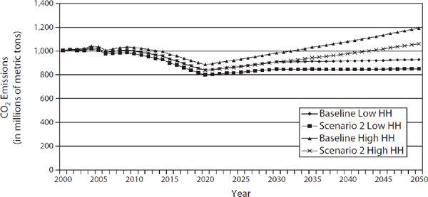
FIGURE D.7 Reduction in CO2 emissions for low to high range of households (HH) from baseline in 2000-2050, assuming 75 percent of all new growth is compact, mixed-use development.
The low and high household values reflect the uncertainty in predicting population growth and replacement housing needs out to 2050. The committee estimates that the number of new housing units would be between 62 million and 105 million units by 2050—this compares to the housing stock of 105.2 million in 2000. The committee assumed no changes to the vehicle fleet beyond the standard proposed in EISA 2007; however, they did run sensitivity analyses to test a doubling of fuel economy by 2050 and found no change in the percent reduction between each scenario. The committee did find that significant fuel economy reductions would far outstrip a reduction in CO2 emissions from VMT only.
Density is likely to lead to changes in vehicle mix and driving conditions that could affect the relationship of VMT to energy use and CO2 emissions. For example, there is evidence that density will encourage the purchase of smaller and hence more fuel-efficient vehicles, so that the reduction in energy use may be more than proportionate to the reduction in VMT. Density may also increase stop-and-go driving and lower speeds under more congested conditions in higher-density areas, which would increase fuel consumption per VMT for conventional vehicles. Such behavioral changes may affect the results; however, the committee believes that these differences are captured in the uncertainties. Final results of the simulations for both scenarios and the baseline are summarized in Table D.9.
D.7 REDUCING GREENHOUSE GAS EMISSIONS FROM U.S. TRANSPORTATION (GREENE AND PLOTKIN, 2011)
This report looks at three scenarios for GHG reduction in the transportation sector. Key technology and policy assumptions for the scenarios as well as the results are described below.
D.7.1 Advanced Vehicles
Building largely on the work of the Massachusetts Institute of Technology report On the Road in 2035 (Bandivedkar et al., 2008), the authors make a case for technological development that could be achieved: new passenger cars could attain 42.8 on-road mpg for gasoline-fueled engines with conventional drivetrains, 48.0 mpg with turbocharging, and 75.9 mpg with hybrid drivetrains. Equivalent values for light-duty trucks are 27.3 mpg, 32.2 mpg, and 49.0 mpg, respectively. The key question in each
TABLE D.9 Assumptions and Results for 2000-2050 Scenarios
| Baseline | 25% New Housing | 75% New Housing | |||||||
| Assumptions | |||||||||
| Housing Units (2000) [#] | 105.2 million | ||||||||
| Housing Units (2050) [#] | 152.9-190.0 million | ||||||||
| VMT per household (existing development) | 21,187 | 21,187 | 21,187 | ||||||
| VMT per household (new noncompact dev.) | +8.4% | +17.5% | |||||||
| 22,967 | 24,895 | ||||||||
| VMT per household (new compact dev.) | −12% | −25% | |||||||
| 20,211 | 18,671 | ||||||||
| Results | |||||||||
| % Increase in VMT between 2000 and 2050 | 50.2%-100% | 48.3%-87.7% | 42.6%-78% | ||||||
| VMT (in billions of miles) 2000 2050 | 2,228.9 | 2,228.9 | 2,228.9 | ||||||
| 3,348.5-4,458.6 | 3,305.5-4,182.8 | 3,177.4-3966.8 | |||||||
| % change in 2050 VMT compared to base case | −1.3% to −1.7% | −8.4% to −11.0% | |||||||
NOTE: Two scenarios are shown (25 percent of new housing at twice the average density and 75 percent of new housing at twice the average density) as well as the baseline projection.
of their proposed scenarios is the degree to which these improvements are made, because while these improvements may be technically achievable, historically most of the efficiency improvements have been nullified by increased performance and additional vehicle mass.
In order to reach the highest levels of fuel efficiency considered in the maximum reductions scenario, alternatively fueled vehicles must be considered. A large number of possible scenarios are conceivable, whether the fuel mix would involve a transition to biofuels, electricity, hydrogen, or a mixture of all three. For biofuel availability, the authors estimate as much as 60 billion gallons could be produced annually in 2050. In the case of electricity, the report cautions against battery electric vehicles due to costs and range anxiety, estimating instead as many as 20 million PHEVs on the road by 2050. With hydrogen, an infrastructure must also be put in place. One clear concern about any of these fuels is that in order to reach significant reduction, they must be generated with low-GHG emissions. For biofuels, this would entail careful tracking of indirect land use change and lifecycle emissions; for electricity, this would mean a shift to a “clean” grid, along with any necessary policies to induce such a shift; for hydrogen, this could mean biomass and coal with CCS instead of steam methane reforming.
D.7.2 System Efficiency
Improving system efficiency offers the potential for significant percent reductions in GHG emissions. However, there is significant debate over the effectiveness of these policies, given the unknown future public response. The authors describe a number of policies to improve system efficiency and reduce GHGs. They estimate that improvements in traffic flow would likely lead to between 0.5 and
1 percent reduction. Reduced trips from ridesharing and car-sharing programs utilized by 1 percent of the population yield GHG emission reduction potentials of 0.2 to 0.6 percent and 0.3 percent, respectively. While ecodriving could improve fuel economy for the average driver by about 10 percent, it is difficult to know to what degree these fuel efficient behaviors would manifest themselves in the public as a whole. Driver awareness also lends itself to proper maintenance, such as maintaining appropriate tire pressure, which could improve total on-road fuel economy by 0.3 percent. Increasingly compact land use is often touted as way to improve efficiency, but this is also the policy with the greatest barriers. The authors find that with appropriate policies, as much as 5 percent reductions in GHG emissions would be possible by 2050, although this would require the greatest acceptance among the public and is only suggested for the “High Reduction” strategy.
D.7.3 Policies to Promote Mitigation
Because GHG emissions reduction is a “public good,” the market will not adequately capture any desired changes unforced. Thus, in order to reduce GHG emissions, policies are necessary. The policies and assumptions of the effectiveness of these policies are outlined in Table D.10. Policies such as fuel economy standards (like CAFE) and fuel standards (e.g., Low Carbon Fuel Standard, Renewable Fuel Standard) may be modeled after programs that are currently in place in this country. However, some of these policies need further clarification.
The main effect of a pricing policy is to suppress demand for a product. It may also be used to incorporate an external cost that the market does not account for. A carbon price of $25 per ton would raise the price of gasoline about 8 percent, reducing vehicle travel by 0.8 percent. Raising the price of fuel by pricing carbon also acts to increase demand for more fuel-efficient vehicles; thus, it can act as a complementary policy to fuel economy standards, encouraging consumers to purchase the vehicles manufacturers are required to make. Pay-as-you-drive insurance is an insurance mechanism that would charge based on the number of miles driven, thus encouraging operators to drive less; pay-at-the-pump has a similar effect but would charge as a function of energy usage and, therefore, encourages more efficient driving as well. Feebates are another way of promoting efficiency—a target vehicle fuel efficiency is set by a governing authority, and those vehicles that surpass it receive a rebate, while those that fall below this efficiency will be assessed a fee, both commensurate with the degree to which they exceed/fall short of the standard. Typically such a program is designed to be revenue-neutral. Because the goal of such policies is to improve the efficiency of vehicles traveling on U.S. roads, it is also important that the highways remain adequately funded as users travel a greater number of miles for a given amount of fuel. Currently, taxes have remained fixed per gallon of gasoline for decades. One way of ensuring a stable revenue source is to index the fuel tax to the efficiency of vehicles on the road.
Results of the scenarios involving the implementation of policies described above are shown in Figure D.8. By 2050, the High, Mid, and Low mitigation scenarios lead to a net decrease of GHG emissions from the transportation sector of 65 percent, 39 percent, and 16 percent, respectively.
D.8 POLICY OPTIONS FOR REDUCING ENERGY USE AND GREENHOUSE GAS EMISSIONS FROM U.S. TRANSPORTATION (TRB, 2011)
Like the study described in the previous section, this TRB study examines policy options across the entire transportation sector; however, it does not describe the implementation of particular levels of policy. In addition to sector-specific policies, the study first explores the effect of economywide carbon pricing. According to several economic models, each employing different assumptions about the costs of developing and deploying emissions-reducing technologies, prices starting at $25 to $75 per CO2-equivalent tonne (CO2e-t) and increasing to $225 to $500 per CO2e-t would be required to achieve an 80 percent reduction in emissions economywide by 2050 (Fawcett et al., 2009). Such a carbon price would
TABLE D.10 Summary of Key Assumptions for Light-Duty Vehicles for the Low, Mid, and High Greenhouse Gas Emissions Mitigation Scenarios
| AEO 2010 (2010-2035) | 2035 | 2050 | |||||||
| Low | Mid | High | Low | Mid | High | ||||
| Change in energy efficiency for total stock (miles per gallon) | 39% | ||||||||
| Fuel economy/emissions standards, % | 15.00 | 30.00 | 40.00 | 35.00 | 60.00 | 80.00 | |||
| Driver behavior and maintenance, % | 2.50 | 5.00 | 10.00 | 2.50 | 5.00 | 10.00 | |||
| Improved traffic flow, % | 0.00 | 1.00 | 2.00 | 0.00 | 1.00 | 2.00 | |||
| Pricing policies | |||||||||
| Carbon price, % | 2.44 | 2.44 | 2.44 | 3.57 | 3.57 | 3.57 | |||
| Road user tax on energy, % | 0.94 | 1.55 | 1.88 | 2.23 | 2.23 | 2.23 | |||
| Pay at the pump insurance, % | 0.00 | 4.37 | 4.37 | 0.00 | 5.20 | 5.20 | |||
| Feebates, % | 0.00 | 10.00 | 10.00 | 0.00 | 10.00 | 10.00 | |||
| Automated highways, % | 0.00 | 0.00 | 1.00 | 0.00 | 0.00 | 5.00 | |||
| Change in vehicle miles traveled (billion vehicle miles traveled) | 54% | ||||||||
| Road user tax on energy, % | −0.19 | −0.49 | −0.64 | −0.39 | −0.77 | −1.03 | |||
| Carbon price, % | −1.20 | −1.20 | −1.20 | −1.74 | −1.74 | −1.74 | |||
| Pay at the pump insurance, % | 0.00 | −0.97 | −0.97 | 0.00 | −0.97 | −0.97 | |||
| Trip planning and route efficiency, % | 0.00 | −2.00 | −4.00 | 0.00 | −5.00 | −10.00 | |||
| Ridesharing, % | 0.00 | −0.70 | −1.40 | 0.00 | −1.00 | −2.00 | |||
| Land use and infrastructure development, % | 0.50 | −1.00 | −2.00 | −1.50 | −3.00 | −5.00 | |||
| Change in fuel carbon intensity for total stock (gCO2e/MJ) | −7% | ||||||||
| LCFS: 2035 / increased hydrogen and electricity: 2050, % | −5.00 | −10.00 | −15.00 | −5.00 | −10.00 | −47.22 | |||
NOTE: The percent change for the Annual Energy Outlook (AEO) 2010 BAU Case from 2010 to 2035 is shown in italics. Values shown in the table reflect percent changes from the AEO value for implementing the respective option. To compare the 2050 values, the AEO 2010 BAU scenario was extrapolated out to 2050 by the authors of the report.
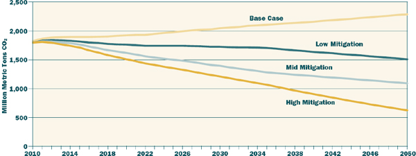
FIGURE D.8 Greenhouse gas emissions from the U.S. transportation sector for different policy scenarios.
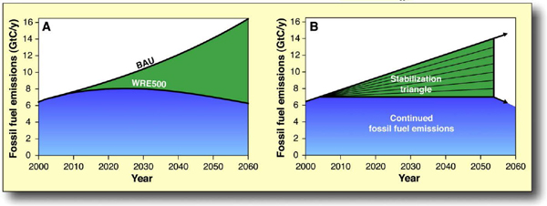
FIGURE D.9 (a) The top curve is a representative emissions pathway, in this case an annual growth of GHG of 1.5 percent. The lower curve models a scenario where GHG emissions would stabilize. (b) is an idealization of (a). The triangle is then broken up into wedges of equal area, each representing a reduction in carbon of 1 gigaton per year.
result in a approximately 20 percent reduction in emissions from the transportation sector alone. However, they also recognize the steep costs this would entail for electricity as well as in the LDV sector, where gasoline prices would be expected to increase about $0.01/gallon per $1/CO2e-t.
D.9 STABILIZATION WEDGES: SOLVING THE CLIMATE PROBLEM FOR THE NEXT 50 YEARS WITH CURRENT TECHNOLOGIES (PACALA AND SOCOLOW, 2004)
The authors of this Science article outline tangible steps the world can take to reduce its fossil fuel emissions modeled on what they term “stabilization wedges” as shown in Figure D.9. There are several suggested activities in the paper—four of them are directly applicable to transportation emissions. Before detailing the strategies, it should be pointed out that these are approaches to mitigating GHG emissions—there are no price-tags associated with these strategies, nor are they meant to be a predictor of the transportation sector of 2054.
D.9.1 Efficient Vehicles
Citing a growth rate of 2.4 percent, the article estimates that in 50 years there will be roughly 2 billion cars on the road globally. If these gasoline-powered vehicles continue to average 10,000 miles per year as they do today, a doubling of fuel economy from 30 mpg to 60 mpg would correspond to the 1 gigaton reduction in carbon emissions necessary for a wedge. The level of fuel economy necessary to reduce GHG emissions by 1 gigaton is highly dependent on the initial level of fuel economy in the base case. If instead of 30 mpg the average fleetwide fuel economy today were 24 mpg, then the entire fleet would only need to achieve 40 mpg in 2050 to achieve a reduction of 1 gigaton of carbon.
D.9.2 Reduced Use of Vehicles
If instead these 2 billion 30-mpg cars reduced their VMT from 10,000 to 5,000 miles, this would also correspond to a 1 gigaton reduction in carbon emissions. Reducing the VMT by such a significant number would likely result in a modal shift towards mass transit, however, which (being another wedge) may result in double-counting of emissions.
D.9.3 Hydrogen-Powered Vehicles
Hydrogen-fueled vehicles offer a low-carbon alternative to gasoline-powered vehicles, enough so that a full transition to a hydrogen-powered fleet provides another wedge of opportunity. However, the way in which the hydrogen fuel is produced determines how much of an offset a complete transition to hydrogen-fueled vehicles yields. The most common mode of generating hydrogen today is part of the fossil-fuel power generation process. However, unless this is combined with carbon sequestration, this is too carbon-rich to provide enough of an offset.
An alternative production mechanism for producing hydrogen is via electrolysis. In this case, however, the authors found that the carbon emissions reductions from using carbon-free electricity that displaces coal and natural gas power plants were significantly larger than using this carbon-free electricity that displaces gasoline and diesel.
D.9.4 Biomass Fuel for Fossil Fuel
The displacement of carbon-rich fossil fuel with biofuels offers another potential wedge. It would require the production of about 34 million barrels per day of ethanol in 2054. This corresponds to roughly 250 million hectares of high-yield plantations (15 dry tons/hectare), or about one-sixth of the world’s cropland. This may be an underestimate to the extent that biofuels require fossil fuel inputs. Because land suitable for annually harvested biofuel crops is also often suitable for conventional agriculture, biofuel production could compromise agricultural productivity. This is, however, a more efficient reduction in carbon emissions possible than if that same land were to be used as a carbon sink.
D.10 TRANSITIONS TO ALTERNATIVE TRANSPORTATION TECHNOLOGIES—A FOCUS ON HYDROGEN (NRC, 2008)
This study looks at the maximum practical number of HFCVs that could be deployed in 2020 and beyond. The committee concluded that “it would not be feasible to have enough hydrogen vehicles on the road by 2020 to significantly affect CO2 emissions and oil use” (p. 3) and thus extended its timeframe out to 2050.
D.10.1 Hydrogen Production
In order to fuel a large hydrogen-powered fleet, hydrogen production will have to be significantly increased. The committee examined four means of producing hydrogen: (1) distributed steam methane reformation (DSMR) using natural gas, (2) centralized hydrogen production from coal gasification, (3) centralized production from biomass gasification, and (4) electrolysis. DSMR from natural gas for onsite production at a refueling station offers an economical first fuel for HFCVs, and even without carbon capture and sequestration (CSS) the well-to-wheels CO2 emissions would be less than half that of a gasoline-powered automobile. However, the cost of DSMR is significantly dependent on the price of
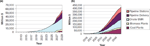
FIGURE D.10 Capital costs for hydrogen infrastructure out to 2030 (a) and 2050 (b).
natural gas, and just 50 million hydrogen-powered vehicles (less than 20 percent of the current fleet) would require a 10 percent increase in natural gas production if it was all generated via DSMR. Centralized hydrogen from coal gasification would require CCS to have a significant impact on CO2 emissions, which also increases its costs. Biomass gasification has much lower emissions than coal, and combined with CCS it would be negative; however, the committee expressed concerns about it being an unproven technology with limits on availability (citing 500 million dry tons, or about 37 billion gallons of gasoline equivalent, 26 percent of the gasoline market). Finally, electrolysis was deemed too expensive to be used in any significant capacity, although the technology is available now. Infrastructure costs associated with these fuels are shown in Figure D.10.
D.10.2 Hydrogen Fuel Cell Vehicles
Because manufacturers have been working on prototype and preproduction HFCVs for a number of years, the committee believes that it is simply a matter of time before hydrogen vehicles are on the market. However, there are still a few technological hurdles to overcome, namely the high cost associated with platinum use in the fuel stack, fuel stack lifetime, and on-board storage. However, based on the amount of R&D money being pumped into HFCV projects, the committee expects full commercialization in the future. The cost for a hydrogen vehicle is shown in Figure D.11a. It is expected that the hefty price tag associated with a hydrogen vehicle would be subsidized by the manufacturer or the government in order to get the market price down to its fully learned out cost. Fuel costs are expected to be competitive with gasoline on a similar time frame (Figure D.11b.. This is expected to lead to a practicable penetration rate of 20 percent of new vehicles by 2035 and 80 percent by 2050, leading to almost 2 million HFCVs on the road in 2020, 60 million in 2035, and more than 200 million in 2050.
D.10.3 Alternative Vehicle Technologies
There are three main paths for reducing gasoline usage proposed in this report: (1) efficiency, (2) HEVs, and (3) biofuels. Via conventional vehicle technologies (including but not limited to lightweighting, aerodynamics, and transmission upgrades), the report estimates that “evolutionary vehicle technologies could, if focused on vehicle efficiency, reduce fuel consumption by 2.6 percent per year through 2025, 1.7 percent per year in the 2025-2035 time frame, and 0.5 percent per year between 2035-2050” (p. 49), resulting in a net decrease in fuel consumption of 48 percent by 2050. Although the committee examined the use of HEVs, they did not consider PHEVs or BEVs to be a sufficiently established technology to develop a framework for analysis (see Section D.11 for a follow-up report). Hybrid vehicles were assumed to maintain their additional 29 percent reduction in fuel consumption
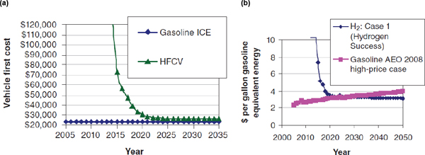
FIGURE D.11 Costs for hydrogen vehicle (a) and fuel (b) compared to gasoline equivalent.
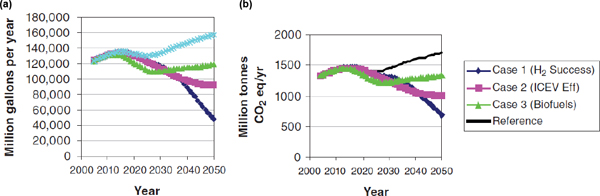
FIGURE D.12 (a) Millions of gallons of oil per year and (b) millions of tonnes CO2 equivalent per year for each of the three scenarios (HFCVs, efficiency, and biofuels).
relative to comparable evolutionary conventional ICEVs. For biofuels, the main concern of the committee was, again, price and availability. The committee estimated that 335 million dry tons per year would be available in the near-term, 490 million dry tons per year by 2030, and as much as 700 million dry tons per year by 2050, although this would require significant technological advancement and potentially high-priced feedstock. This would result in an upper bound of 63 billion gallons of ethanol producible in 2050.
D.10.4 Greenhouse Gas Emissions
The committee examined three scenarios that offered substantial CO2 emissions reductions by 2050: (1) HFCVs, (2) improved vehicle efficiency (including HEVs), and (3) biofuels. Figure D.12 shows reduction in oil (panel a) and GHG emissions (panel b) for each of these scenarios.
In addition to these scenarios, combinations of technologies were also examined. For example, a combination of efficiency and biofuels yields similar oil and GHG reductions to the HFCV case. Final results for all studies are shown in Table D.11.
TABLE D.11 Gasoline Displacement and GHG Emission Reductions for All Cases Compared to Reference
| Scenario | Billion Gallons Gasoline Saved/yr (%) | Millions Tonnes CO2 Avoided (%) | |||||||
| 2020 | 2035 | 2050 | 2020 | 2035 | 2050 | ||||
| HFCVs | 1.0 (0.8%) | 34 (24%) | 109 (69%) | 10 (0.7%) | 295 (19%) | 1026 (60%) | |||
| Efficiency | 2.2 (1.7%) | 35 (25%) | 64 (41%) | 24 (1.7%) | 385 (25%) | 700 (41%) | |||
| HFCVs + Efficiency | 3.0 (2.2%) | 55 (39%) | 125 (80%) | 26 (1.8%) | 475 (31%) | 1123 (66%) | |||
| Biofuels | 12 (9%) | 28 (20%) | 39 (25%) | 118 (8%) | 281 (18%) | 386 (23%) | |||
| Efficiency + Biofuels | 14 (11%) | 64 (45%) | 103 (66%) | 143 (10%) | 666 (44%) | 1086 (64%) | |||
| Portfolio (All Options) | 15 (11%) | 83 (59%) | 157 (100%) | 130 (9%) | 747 (49%) | 1505 (88%) | |||
TABLE D.12 Estimated Future Incremental (Compared to Nonhybrid) Costs of PHEVs (to the Manufacturer)
| 2011 | 2015 | 2020 | 2030 | ||||||
| PHEV-40 | 14,100-18,100 | 11,200-14,200 | 9,600-12,200 | 8,800-11,000 | |||||
| PHEV-10 | 5,500-6,300 | 4,600-5,200 | 4,100-4,500 | 3,700-4,100 | |||||
D.11 TRANSITIONS TO ALTERNATIVE TRANSPORTATION TECHNOLOGIES—PLUG-IN HYBRID ELECTRIC VEHICLES (NRC, 2010b)
PHEVs were not included in the original analysis of this committee (NRC, 2008; see Section D.10) because of the speculative nature of any discussion regarding this emerging technology. However, this follow-on study returned to that issue to study the impacts of PHEVs within the scenarios outlined above. Here the committee considered two types of PHEV—a Toyota Prius-like PHEV with an all-electric range of 10 miles (which will be abbreviated as PHEV-10) and a Chevrolet Volt analog with an all-electric range of 40 miles (PHEV-40). The PHEV-10 has a smaller electric motor, so the gasoline engine is engaged in high-power situations as well as when the vehicle is running in charge-sustaining mode (similar to standard hybrid operation). In contrast, the PHEV-40 only runs in charge-sustaining mode when the battery has been fully depleted.
D.11.1 Battery Packs for PHEVs
Because Li-ion battery technology is well-adopted in the consumer electronics market (cell phones, laptop batteries, etc.), the committee felt that the steep drop in price typically associated with volume-based learning would not occur for the PHEV battery packs, leading to a slow reduction in price over time (Table D.12). The committee further noted that while breakthroughs in battery technology offer the potential to greatly lower the cost, it is not clear what sorts of breakthroughs may occur and, even if they did, whether they would be able to have much impact by 2030. While simply increasing the available state of charge (SOC) from 50 to 80 percent would lower the cost of the battery substantially, it was felt that there were significant potential risks to the longevity and safety of the battery, so the committee did not include changes to the available SOC in their cost reductions.
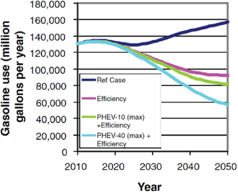
FIGURE D.13 Gasoline use for PHEV scenarios.
D.11.2 Market Penetration
Because of the high cost of batteries, the committee expressed concern over the ability for PHEVs to penetrate the market. They put forward two scenarios—the first is the probable market penetration, without subsidization and giveaways; the second is the maximum possible penetration of PHEVs, which would require policy initiatives such as subsidies, fuel economy standards, or carbon pricing. In the probable scenario, 3 percent of new vehicles sold in 2020 and 15 percent in 2035 would be PHEVs, leading to 110 million PHEVs on the road by 2050. This rate of penetration was determined by selecting the “probable” incremental costs of PHEVs, which do not find a payback period for PHEVs within a timeframe appropriate for the consumer, given gasoline prices less than $4 per gallon. In the maximum practical scenario, the committee used the same maximum sales rate as in the previous study for HFCVs (see Section D.10), resulting in a fleet of approximately 240 million PHEVs by 2050. Here they assumed the lowest anticipated future costs, noting that “if costs fail to decline to those levels, this scenario would be prohibitively expensive” (p. 24).
D.11.3 Petroleum and Greenhouse Gas Reductions
A PHEV gets its fuel economy benefits from the fact that the vehicle is using an electric motor for a substantial fraction of its mileage. However, GHG emissions from the vehicle are only reduced if the upstream emissions from the power plants acting as a “fuel source” for this battery are cleaner than the gasoline it is displacing. To analyze the potential GHG reductions under widespread PHEV adoption, the committee considered a number of different scenarios, as in the previous study (see Section D.10.4), as well as two different projected electrical grids, a BAU grid from the Energy Information Administration (EIA) and a “clean grid” adapted from the Electric Power Research Institute (EPRI) and the National Resource Defense Council (NRDC).
In the case of the PHEV-10, the vehicle runs 81 percent of its miles on the gasoline engine, meaning that it does not result in significant petroleum reductions compared to a normal HEV (just 7 percent additional reduction). This is reflected in Figure D.13, which compares the maximum practical PHEV-10 and PHEV-40 scenarios with the base efficiency and reference cases. Here the PHEV scenarios are combined with the efficiency case under the assumption that PHEVs would not make significant market gains until other efficiency measures have been enacted because of the costs associated with implementing this technology in the fleet.
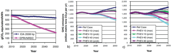
FIGURE D.14 (a) Comparison of the Energy Information Administration (EIA) business-as-usual grid and the Electric Power Research Institute (EPRI)/National Resource Defense Council (NRDC) clean grid. Greenhouse gas (GHG) emissions for the PHEV scenarios are shown for the two grids: (b) EIA BAU grid (2050: PHEV-10 max = 1170 Mmt CO2, PHEV-40 max = 1100 Mmt CO2); (c) EPRI/NRDC clean grid (2050: PHEV-10 max = 1090 Mmt CO2, PHEV-40 max = 890 Mmt CO2).
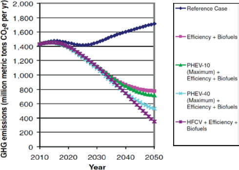
FIGURE D.15 Comparison of maximum practicable PHEV scenarios with biofuels and efficiency, in the clean grid case.
The significance of the grid in adoption of PHEVs is shown in Figure D.14. A cleaner grid increases the spread in the PHEV-10 and PHEV-40 emissions because of the higher fraction of VMT on electricity (19 percent for the PHEV-10 and 55 percent for the PHEV-40) and increases the available decrease in GHG emissions for the PHEV-40 (PHEV-10) from 35 percent (31 percent) to 48 percent (36 percent) by 2050.
The maximum practicable scenario for a clean grid, efficiency, and biofuels is shown in Figure D.15. Here it is also compared to the hydrogen case (Section D.10) with similarly available technologies. While efficiency and biofuels alone make up the majority of the reductions in all cases by 2050 (55 percent), PHEV-10s (59 percent) and PHEV-40s (71 percent) offer significant additional reductions, although short of the possible reductions from HFCVs calculated by the hydrogen study committee (80 percent) (Section D.10).
D.12 ENVIRONMENTAL ASSESSMENT OF PLUG-IN HYBRID ELECTRIC VEHICLES, VOLUME 1 (EPRI AND NRDC, 2007)
EPRI and the NRDC examined the potential for GHG reductions due to the widespread adoption of PHEVs. The study looked at the timeframe of 2010 (when they assumed PHEVs would first hit the market) to 2050.
D.12.1 Power Generation
PHEVs can be thought of as a dual-fuel vehicle—any reduction in GHG emissions relative to a normal hybrid will have to come as a function of use of the secondary fuel (electricity) and its carbon intensity. Therefore, this study first examined the carbon intensity of the grid from 2010-2050 using EIA’s National Energy Modeling System and EPRI’s own National Electric System Simulation Integrated Evaluator.
Three scenarios were considered—a low-, medium-, and high-CO2 scenario—each representing a different projection of the electrical grid of the future. In the high-CO2 scenario, there is not a significant adoption of renewable and other low-GHG-emitting power generation sources. Furthermore, there is no economic incentive (such as cap-and-trade or a carbon tax) for producers to de-carbonize power production. In this case, total GHG emissions from the grid increase by 25 percent by 2050. In the medium-CO2 scenario, there is a moderate cost of carbon that helps push adoption of low-CO2 energy sources as well as greater technological advancement allowing for biomass plants and CCS on new plants. This results in a decrease in total GHG emission by 41 percent between 2010 and 2050. Finally, the low-CO2 scenario represents the greatest adoption of low-CO2 energy sources as well as the most advanced technology, allowing for retrofits of “dirty” coal plants with CCS and greater efficiencies of renewable energy sources. This results in a net decrease in GHG emissions from power generation of 85 percent. The assumptions leading to these scenarios are given in Table D.13.
TABLE D.13 Key Parameters of Power Generation Scenarios
| Scenario Definition | High CO2 Intensity | Medium CO2 Intensity | Low CO2 Intensity | ||||||
| Price of greenhouse gas emission allowances | Low | Moderate | High | ||||||
| Power plant retirements | Slower | Normal | Faster | ||||||
| New generation technologies | Unavailable: Coal with CCS New nuclear New biomass | Available: IGCC coal with CCS New nuclear New biomass Advanced renewables | Available: Retrofit of CCS to existing IGCC and PC plants | ||||||
| Lower performance: SCPC, CCNG, GT, wind, and solar | Nominal EPRI Performance Assumptions | Higher performance: Wind and solar | |||||||
| Annual electricity demand | 1.56% per year on | 1.56% per year on | 2010-2025: 0.45% | ||||||
| growth | average | average | 2025-2050: None | ||||||
NOTE: PC = pulverized coal; CCNG = combined cycle natural gas; CCS = carbon capture and storage; SCPC = supercritical pulverized coal; GT = gas turbine (natural gas).
TABLE D.14 Peak New Vehicle Market Share in 2050 for the Three PHEV Adoption Scenarios
| 2050 New Vehicle Market Share by Scenario | Vehicle Type | ||||||||
| Conventional | Hybrid | Plug-In Hybrid | |||||||
| PHEV Fleet | Low PHEV | 56% | 24% | 20% | |||||
| Penetration Scenario | Fleet Penetration | ||||||||
| Medium PHEV | 14% | 24% | 62% | ||||||
| Fleet Penetration | |||||||||
| High PHEV | 5% | 15% | 80% | ||||||
| Fleet Penetration | |||||||||
| Baseline Fleet | Low PHEV | 70% | 30% | 0% | |||||
| Penetration Scenario | Fleet Penetration | ||||||||
| Medium PHEV | 37% | 63% | 0% | ||||||
| Fleet Penetration | |||||||||
| High PHEV | 25% | 75% | 0% | ||||||
| Fleet Penetration | |||||||||
D.12.2 Market Penetration
EPRI and NRDC determined that PHEVs would be applicable not just in the light-duty gasoline and diesel vehicle sector but also to heavy-duty vehicles up to 19,500 pounds (Class 5). Three different scenarios for PHEV penetration into these sectors by 2050 were considered (Table D.14). The penetration scenario is characterized by the familiar S-shape, with the majority of adoption occurring by 2020. It is also assumed that the share of PHEV-20s and PHEV-40s within the PHEV class will grow over time. The baseline case represents what the scenario would look like in the absence of PHEVs, yielding the same ratio of HEVs to conventional vehicles as in the PHEV penetration scenario.
D.12.3 Results
Figure D.16 shows the relative GHG emissions for conventional, hybrid electric, and PHEVs with a 20-mile all-electric range (PHEV-20). Included in the PHEV values are the upstream emissions from different types of power plants. This graph shows the significance of the carbon intensity of the grid itself on the effectiveness of the PHEV at reducing GHG emissions. Figure D.16 shows the values in 2050 given the deployment of advanced low-CO2 power generators. These values also incorporate increases in fuel economy in conventional and hybrid vehicles.3
Table D.15 shows the annual CO2 reduction from PHEVs in 2050 in each of the nine scenarios. Even in the highest carbon grid case, they find significant potential for GHG reductions with a net market penetration of 20 percent. The cumulative CO2 reductions amount to between 3.4 and 10.3 billion tons of carbon between 2010 and 2050.
_____________________________
3 When the PHEV is running in charge-sustaining mode, it is assumed that it will have the same fuel economy as a hybrid vehicle. The hybrid is assumed to have 35 percent better fuel consumption than a similar conventional vehicle. Fuel consumption is projected to improve for all vehicles at a rate of 0.5 percent per year.
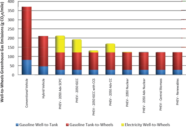
FIGURE D.16 Year 2050 comparison of greenhouse gas emissions from a light-duty, gasoline-power PHEV-20 when charged entirely with electricity from specific power plant technologies (assuming 12,000 miles driven per year).
TABLE D.15 Annual CO2 Reductions in 2050 for the Nine Analyzed Scenarios
| 2050 Annual CO2 Reductions (million tons) | Electric Sector CO2 Intensity | ||||||||
| High | Medium | Low | |||||||
| PHEV Fleet | Low | 163 | 177 | 193 | |||||
| Penetration Scenario | Medium | 394 | 468 | 478 | |||||
| High | 474 | 517 | 612 | ||||||
D.13 STRATEGIES FOR REDUCING THE IMPACT OF SURFACE TRANSPORTATION ON GLOBAL CLIMATE CHANGE (BURBANK, 2009)
This study was commissioned by the American Association of State Highway and Transportation Officials as part of the National Cooperative Highway Research Program through the TRB and examines the ability of the United States to reduce GHG emissions in the transportation sector. A significant reduction in transportation GHGs (70 percent below 2005 levels by 2050) was analyzed in this study based on state-adopted and federally proposed targets for total GHG emissions reductions. In order to meet this level, the authors focused on four potential areas of reduction: (1) vehicle technologies, (2) alternative fuels, (3) VMT, and (4) vehicle/system operations.
TABLE D.16 Year 2050 Scenarios Evaluated; Change in Emissions Compared to 2005
| Scenario Concept Description | GHG emission reduction per mile | Annual Change to VMT | Operational Efficiency Improvements by 2050 | 2050 GHG % Change compared to 2005 Baseline | |||||
| Baseline forecast from DOE AEO 2008 | 41% | +1.74% | None | +11% | |||||
| “Stretch” fleet GHG efficiency and 1% VMT | 79% | +1.0% | 10% | −76% | |||||
| AASHTO approximated scenario with more aggressive operational efficiency improvements | 72% | +1.0% | 15% | −69% | |||||
| AASHTO approximated scenario with improved operational efficiency improvements | 72% | +1.0% | 10% | −64% | |||||
| Improved fleet GHG efficiency; near-zero VMT per capita increase | 72% | +0.9% | 10% | −66% | |||||
| Fleet GHG efficiency; near-zero VMT per capita increase | 58% | +0.9% | 10% | −44% | |||||
| Fleet GHG efficiency; more aggressive operational improvements; lowest VMT growth | 58% | +0.5% | 15% | −56% | |||||
SOURCE: Adapted from Burbank (2009), Table 3.1.
D.13.1 Light-Duty Vehicle Scenarios
In order to ascertain future directions of policy and the potential for GHG reductions in the transportation sector, a series of projected scenarios were carried out looking forward to GHG emissions in 2050. They assumed some amount of operational efficiency improvements (e.g., traffic smoothing, “ecodriving”) in every scenario but the BAU baseline case. Each scenario offers varying levels of vehicle efficiency and VMT. Results are summarized in Table D.16.
The baseline case results in an increase in GHG emissions due to increased VMT despite a 41 percent reduction in efficiency. Only one scenario (that requiring a 100 mpgge fleet, shown in Figure D.17) was shown to meet the 70 percent GHG reduction benchmark according to the study. With significant improvements in operational efficiency, a less aggressive efficiency mark (75 mpgge, just slightly lower than the study’s estimated efficiencies for available fuel cell and PHEVs) would nearly meet this 70 percent target as well.
D.13.2 Medium-and Heavy-Duty Vehicle Scenarios
The projected scenarios for the medium-and heavy-duty vehicles are significantly less complicated than that for the LDVs. The baseline scenario was developed first from the EIA’s Annual Energy Outlook (AEO) from 2008, which showed an annual increase in VMT for medium-and heavy-duty trucks of about 1.68 percent. The average annual increase in energy consumption by the fleet in the EIA AEO 2008 from 2005 to 2030 was then extrapolated out to 2050. The energy consumption was converted to GHG emissions using the fuel mix for the fleet. The baseline case does include proposed fuel economy standards from the EISA 2007 and the Renewable Fuel Standard. The percentage of fuels by fuel type from 2031 to 2050 was assumed to be the same as percentages of fuel by fuel type in 2030.
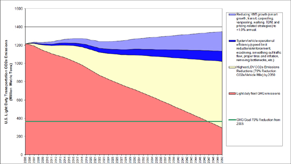
FIGURE D.17 Scenario 1—1 percent vehicle miles travelled (VMT) growth, 100 mpgge LDV fleet in 2050, improving operational efficiency.
A second scenario was projected that saw marked fuel efficiency improvements in the medium-and heavy-duty fleet. These improvements are based on the 21st Century Truck Program, which includes the development and demonstration of heavy-duty hybrid propulsion technology. A rapid fleetwide transition to this technology is assumed by 2030; this trend was projected out to 2050, resulting in a net efficiency improvement of 133 percent. However, even with these efficiency gains, the net GHG emissions for the medium-and heavy-duty fleet are barely sufficient to counter the increase in GHG emissions due to increasing VMT (Figure D.18).
D.14 ASSESSMENT OF FUEL ECONOMY TECHNOLOGIES FOR LIGHT-DUTY VEHICLES (NRC, 2011)
The Committee on the Assessment of Technologies for Improving Light-Duty Vehicle Fuel Economy was faced with the task of assessing the costs of LDV technologies that might be used to reduce fuel consumption in vehicles over the next 15 years, including significant changes to the powertrain and advanced lightweighting. Homogeneous-Charge Compression Ignition (HCCI) engines are a technology that has been perennially 10 years on the horizon, and it was deemed by the committee to be beyond the 15-year scope of the study. Advanced diesel is available today in the United States, but the committee felt that much of the fuel consumption benefit will be offset by fuel consumption increases in the future (2014-2020) to meet more stringent emissions standards. While there are fully electric battery-powered vehicles in the marketplace today, the committee found that the most likely electrification scenario over the next 15 years would be for range-extended electric vehicles to make major inroads due to high battery costs forcing a limited range and/or extremely high costs for BEVs without breakthrough technology. While the committee noted that every major original equipment manufacturer (OEM) has a fuel cell vehicle program, through interviews and presentations they found little evidence that a commercially viable fuel cell vehicle will be available in significant numbers by 2020. Furthermore, the difficulty of providing the hydrogen infrastructure necessary to support HFCVs and other factors suggested to the committee that there would not be wide use of fuel cell vehicles before 2025. Finally, in regards to
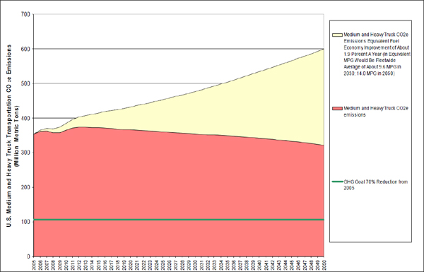
FIGURE D.18 Truck Fleet Efficiency Improvement Scenario: Annual VMT of 1.68 percent and 14 mpgge in 2050.
lightweighting, while the committee made no long-term projection of how light a vehicle could get, they noted that achieving a mass reduction of 10-20 percent will require a significant change in vehicle design, which will in turn increase costs. The uncertainty and instability of commodity prices (e.g., for aluminum or carbon fiber compared to steel) also increase the risk to OEMs of adopting these new materials.
D.15 LIGHT-DUTY VEHICLE FUEL CONSUMPTION DISPLACEMENT POTENTIAL UP TO 2045 (ANL, 2011)
The Vehicle Modeling and Simulation group at Argonne National Laboratory prepared a report that examined the technologies likely to be implemented by 2045 and the costs associated with them in order to evaluate the breadth of LDV technologies and ensure that the DOE is focusing its research on the most promising technologies. In order to simulate the uptake of the technologies, the researchers modeled vehicles packaged using various vehicle technologies. In all, more than 2,000 different vehicles were simulated. These different vehicles were chosen to simulate the various combinations of powertrain (i.e., power-split hybrid, conventional, full-electric) and fuel (i.e., gasoline, E85, diesel) available for each of the five vehicle classes (compact and midsize cars, small and large SUVs, and pick-up trucks).
Among its key findings, the report concludes that significant weight reductions (up to 37 percent in the most optimistic scenario) can be achieved by 2045, compared to current state of the art, especially for vehicles with large batteries and/or using hydrogen fuel. Owing to this, the peak power of engines/motors can be reduced significantly over time while maintaining current vehicle technical specifications.
FIGURE D.19 Simulated total fuel use (a) and GHG emissions (b) for the US LDV fleet in 2050.
The most prominent conclusion is that due to expected improvements, this report finds that advanced technologies are expected to have significant market penetration. In the short term (to 2015), HEVs and PHEVs offer significant fuel displacement with an acceptable additional cost; however, BEVs are likely to remain expensive and range-limited, hindering their initial market penetration. In the medium term (to 2030), hybridized hydrogen-fueled ICE-powered vehicles would offer significant fuel improvements and could potentially act as a bridging technology to establish the infrastructure required for fuel cell vehicles. In the long term (to 2045), fuel cell vehicles demonstrate the highest fuel displacement potential at a competitive cost.
D.16 THE EFFECT OF UNCERTAINTY ON U.S. TRANSPORT-RELATED GHG EMISSIONS AND FUEL CONSUMPTION OUT TO 2050 (BASTANI ET AL., 2012)
Bastani, Heywood, and Hope employed a deterministic model to shed light on the likely future of LDVs in 2050. The scenarios given by the model are based around the statistical uncertainty of key parameters driving future deployment, such as vehicle technology performance, fuel performance and GHG emissions, alternative fuel availability, and demand and market deployment of new technologies and fuels. Tens of thousands of “futures” are considered via Monte Carlo simulation using parameter values obtained via a thorough review of the literature.
Figure D.19 shows simulated fuel use and GHG emissions for the simulated scenarios. While these values are meant to represent likely scenarios for future LDV pathways, which is inconsistent with the committee’s task, they do show both the high potential for significant reductions in oil use and GHG emissions from efficiency improvements as well the high degree of uncertainty in any such modeling endeavor.
Figure D.20 outlines the most significant parameters affecting the future GHG emissions of the light duty fleet, according to the statistically modeled scenarios. The most significant contribution is the uncertainty in future vehicle sales, as should be obvious since the number of vehicles is directly proportional to the GHG emissions of the fleet. This is followed by the percentage of cellulosic ethanol in future gasoline, which has a strong impact on the well-to-wheel emissions of the fleet. There is a comparable strong dependence on the emphasis on reducing fuel consumption (ERFC). The ERFC represents the relative importance of fuel consumption as engines are improved—for example, in the 1990s the ERFC was near zero, while engine improvements were devoted primarily to increasing horsepower. Because the future fleet is dominated by spark-ignited ICE vehicles, the relative fuel
FIGURE D.20 Major influences on the simulated GHG emissions for the U.S. LDV fleet in 2050.
consumption of such vehicles is also a significant contributor. Scrappage is another strong contributor because it helps set the rate at which new technology penetrates the fleet. Because plug-in and HEVs are not expected to be a significant fraction of the fleet in this work, assumptions about their sales and the emissions from the grid are much less significant to future scenarios than VMT or well-to-wheels emissions from gasoline.
D.17 REFERENCES
An, F., and D. Santini. 2004. “Mass impacts on fuel economies of conventional vs. hybrid electric vehicles.” SAE Technical Paper 2004-01-0572. Warrendale, Pa.: SAE International.
ANL (Argonne National Laboratory). 2011. Light-Duty Vehicle Fuel Consumption Displacement Potential Up to 2045. ANL/ESD/11-4. Argonne, Ill.: Energy Systems Division, Argonne National Laboratory. July.
Bandivadekar, A.P., K. Bodek, L. Cheah, C. Evans, T. Groode, J. Heywood, E. Kasseris, K. Kromer, and M. Weiss. 2008. On the Road in 2035: Reducing Transportation’s Petroleum Consumption and Greenhouse Gas Emissions. Laboratory for Energy and the Environment Report No. LFEE 2008-05 RP. Cambridge, Mass.: Massachusetts Institute of Technology. July.
Bastani, P., J.B. Heywood, and C. Hope. 2012. The effect of uncertainty on U.S. transport-related GHG emissions and fuel consumption out to 2050. Transportation Research, Part A: Policy and Practice 46(3):517-548.
Burbank, C.J. 2009. Strategies for Reducing the Impact of Surface Transportation on Global Climate Change. Prepared for the American Association of State Highway and Transportation Officials. Washington, D.C.: Parsons Brinckerhoff. February.
Cheah, L., and J. Heywood. 2008. “Meeting CAFE standards by 2020 and beyond.” Research Brief, Sloan Automotive Laboratory. Cambridge, Mass.: Massachusetts Institute of Technology. November.
Cheah, L., C. Evans, A. Bandivedkar, and J. Heywood. 2007. Factor of Two: Halving the Fuel Consumption of New U.S. Automobiles by 2035. Laboratory for Energy and the Environment Report No. LFEE 2007-04 RP. Cambridge, Mass.: Massachusetts Institute of Technology.
DOT (U.S. Department of Transportation). 2010. Transportation’s Role in Reducing U.S. Greenhouse Gas Emissions. Volumes 1 and 2. Report to Congress. Prepared by the Center for Climate Change and Environmental Forecasting. Washington, D.C. April.
EPRI (Electric Power Research Institute) and NRDC (Natural Resource Defense Council). 2007. Environmental Assessment of Plug-In Hybrid Electric Vehicles—Volume 1: Nationwide Greenhouse Gas Emissions. Palo Alto, Calif.: EPRI. July.
Fawcett, A.A., K.V. Calvin, F.C. de la Chesnaye, J.M. Reilly, and J.P. Weyant. 2009. Overview of EMF 22 U.S. transition scenarios. Energy Economics 31: S198-S211.
Greene, D.L., and S.E. Plotkin. 2011. Reducing Greenhouse Gas Emissions from U.S. Transportation. Prepared for the Pew Center on Global Climate Change. Arlington, Va. January.
Kromer, M.A., and J.B. Heywood. 2007. Electric Powertrains: Opportunities and Challenges in the U.S. Light Duty Vehicle Fleet. MIT publication LFEE 2007-02 RP. Available at http://web.mit.edu/sloan-auto-lab/research/beforeh2/files/kromer_electric_powertrains.pdf.
McCollum, D., and C. Yang. 2009. Achieving deep reductions in U.S. transport greenhouse gas emissions: Scenario analysis and policy implications. Energy Policy 37(12):5580-5596.
NPC (National Petroleum Council). 2007. “Technologies for transportation efficiency.” Topic paper of the Transportation Efficiency Subgroup. Council Committee on Global Oil and Gas. Washington, D.C.: NPC. July.
NRC (National Research Council). 2004. The Hydrogen Economy: Opportunities, Costs, Barriers, and R&D Needs. Washington, D.C.: The National Academies Press.
———. 2008. Transitions to Alternative Transportation Technologies: A Focus on Hydrogen. Washington, D.C.: The National Academies Press.
———. 2009a. Liquid Transportation Fuels from Coal and Biomass—Technological Status, Costs, and Environmental Impacts. America’s Energy Future Series. Washington, D.C.: The National Academies Press.
———. 2009b. Real Prospects for Energy Efficiency in the United States. America’s Energy Future Series. Washington, D.C.: The National Academies Press.
———. 2010a. Limiting the Magnitude of Future Climate Change. America’s Climate Choices Series. Washington, D.C.: The National Academies Press.
———. 2010b. Transitions to Alternative Transportation Technologies—Plug-in Hybrid Electric Vehicles. Washington, D.C.: The National Academies Press.
———. 2011. Assessment of Fuel Economy Technologies for Light-Duty Vehicles. Washington, D.C.: The National Academies Press.
Pacala, S., and R. Socolow. 2004. Stabilization Wedges: Solving the Climate Problem for the Next 50 Years with Current Technologies. Science 305(5686):968-972. August 13.
TRB (Transportation Research Board). 2010. Driving and the Built Environment: Effects of Compact Development on Motorized Travel, Energy Use, and CO2 Emissions. Special Report 298. Washington, D.C.: The National Academies Press.
———. 2011. Policy Options for Reducing Energy Use and Greenhouse Gas Emissions from U.S. Transportation. Special Report 307. Washington, D.C.: The National Academies Press.
UCD (University of California, Davis). 2011. Sustainable Transportation Energy Pathways: A Research Summary for Decision Makers (J. Ogden and L. Anderson, eds.). Davis, Calif.: Institute of Transportation Studies.
Wohlecker, R., M. Johannaber, and M. Espig. 2007. “Determination of weight elasticity of fuel economy for ICE, hybrid and fuel cell vehicles.” SAE Technical Paper 2007-01-0343. Warrendale, Pa.: SAE International.


