
This appendix is an addendum to Chapter 2 of the main report, providing additional information on subjects discussed there. Section F.1 discusses efficiency technologies for internal combustion engine (ICE) vehicles (ICEVs) and hybrid electric vehicles (HEVs). Some of these technologies also apply to other types of vehicles. Section F.2 discusses the modeling techniques uses to estimate future fuel consumption. Two spreadsheet models are also included in the electronic version of this appendix. The Vehicle Input Spreadsheet shows the committee’s estimates of the reduction in energy losses over time for the six vehicles analyzed. The Vehicle Cost Summary estimates the cost of the various vehicles analyzed (6 models each of ICEVs, HEVs, battery-powered electric vehicles [BEVs], and hydrogen fuel cell electric vehicle [FCEVs]). Section F.3 elaborates on the battery vehicle section of Chapter 2, and Section F.4 on the hydrogen fuel cell electric vehicle section.
F.1 EFFICIENCY TECHNOLOGIES FOR CONVENTIONAL VEHICLES
F.1.1 Load Reduction Technologies Applicable to All Vehicles
F.1.1.1 Mass Reduction
This discussion is focused on the potential benefits of reducing the mass of vehicles to improve fuel economy. The government’s fuel economy standards are footprint based and provide no incentive for downsizing vehicles. Potential effects on safety, fuel economy, and vehicle costs are discussed for scenarios where mass reduction is accomplished entirely through material substitution and smart design that can reduce mass without changing a vehicle’s functionality or safety performance and maintains structural strength.
Fuel Economy Benefits
The engineering rule of thumb, assuming appropriate engine resizing is applied and vehicle performance is held constant, is that a 10 percent curb weight reduction results in a 6-7 percent fuel consumption savings (NHTSA-EPA, 2010). For this committee’s analysis, the fuel consumption from weight reduction is calculated as one of the inputs into an energy audit model.
Potential for Mass Reduction
The National Highway Traffic Safety Administration (NHTSA) and the Environmental Protection Agency (EPA) examined mass reductions of 15-30 percent for the 2017-2025 timeframe (NHTSA-EPA, 2010). The automobile manufacturers’ position, as characterized in the Technical Assessment Report (TAR), was that mass reduction plans for 2017-2025 were focused on increased use of high strength steel and some additional aluminum with resulting mass reductions of 10-15 percent. Manufacturers generally
indicated that universal material substitution (such as a switch from steel to aluminum body in white (BIW)1 structures) would not be feasible across all body lines in the 2017-2025 timeframe. In the TAR covering 2017-2025 Model Years, the government stated that “the ability of the industry to reduce mass beyond 20% while maintaining vehicle size … is an open technical issue” (EPA-NHTSA-CARB, 2010, p. 3-8).
The Partnership for New Generation Vehicles research effort from 1994-2002 was an early effort to conceptualize and build highly fuel efficient vehicles. The mass reduction goal was 40 percent. Actual vehicles achieved a mass reduction of 20 to 30 percent (NRC, 2001).
A recent study by the University of Aachen, done for the European Aluminum Association, looked at weight reduction opportunities for aluminum versus steel for subcompact and medium-sized passenger vehicles, crossover vehicles, and small multi-purpose vehicles. The Aachen study looked at optimizing the BIW and closures with aluminum intensive designs and concluded that a 40 percent weight savings in these areas was possible. BIW and Closure Reductions of 40-45 percent translate to an incremental (taking into account aluminum content already in standard production vehicles) 10-11 percent total vehicle weight reduction and with secondary weight savings yield approximately a 15 percent reduction in total vehicle weight (Aachen, 2010).
The 15 percent weight reduction of the total vehicle was repeated in detailed design studies by IBIS Associates, Inc., although secondary weight savings and use of lightweight materials in the rest of the body would result in much greater overall weight savings (IBIS, 2008). An interesting aspect of the Aachen study is that it looked specifically at the use of the aluminum-intensive parts from the standpoint of vehicle stiffness (handling, comfort, noise) and strength needed for managing crash energies and constrained the proposed design to meet or exceed current vehicle BIW performance when it quantified weight reduction opportunities.
Lotus showed similar conclusions to the Aachen study regarding BIW weight savings (Lotus, 2010). The Lotus study evaluated the total vehicle design and hypothesized a “high development” vehicle using an aluminum/magnesium intensive design with an overall weight reduction of about 40 percent. The primary areas of mass reduction are:
- Body in white and closures—44 percent,
- Interior—20 percent, and
- Suspension/chassis—33 percent.
The aluminum industry sponsored studies, which looked strictly at weight reduction for the BIW and closures with associated secondary weight reduction, are in agreement with the Lotus study for similar areas of the vehicle. Lotus also used increased aluminum as part of the suspension and chassis optimized design.
Polymer-matrix composites (PMC, e.g., carbon fiber) have the potential to make a significant further contribution to reducing mass if the production costs of such materials can be reduced with mass production. “Conservative estimates are that carbon fiber PMC can reduce the mass of a steel structure by 40-50 percent …” (NRC, 2011, p. 102). However, there are currently production concerns for using carbon fiber in mass-produced vehicles. Currently, there still is not a known substitute for the existing carbon fiber process, which is too expensive for high-volume applications. Because of this uncertainty, the committee has not included carbon fiber in the 2050 mass reduction scenarios.
A key factor when evaluating design strategies for reducing mass is the corresponding secondary weight savings from rationalizing chassis, suspension, and drivetrain performance for the reduced mass. Estimates of the synergistic effects of mass reduction and the compounding effect that occurs along with it can vary significantly. In comments to various U.S. Corporate Average Fuel Economy (CAFE) rulemaking proposals, the Auto-Steel Partnership estimates that these secondary mass changes can save
_____________________________
1Body in white is the term for the stage in vehicle manufacture when all the fixed sheet metal components are fastened together. It does not include moveable parts such as doors, hood, and trunk (closures).
an additional 0.7 to 1.8 times the initial mass change. Comments by the Aluminum Transportation Group have estimated a factor of 64 percent for secondary mass reduction (NHTSA, 2010). The 2011 National Research Council (NRC) report Assessment of Fuel Economy Technologies for Light-Duty Vehicles pointed out the importance of secondary weight reduction “as the mass of a vehicle is reduced … other components of the vehicle can be reduced … for example brakes, fuel system, powertrain, and even crash management structures” (NRC, 2011, p. 113). It discussed a rule of thumb that for every pound saved in the design through material substitution or structural modifications, an additional 30 percent of the weight savings in secondary systems could be saved (NRC, 2011).
Potential Cost Impacts
Cost estimates for reducing vehicle mass have varied significantly. One difference is the cost savings from secondary weight reduction which can offset some of the costs related to lightweight materials and improved structural design. In this context, the net costs for mass reduction should include the secondary weight and drivetrain downsizing that are directly related to mass efficient vehicle designs. The impacts of weight reduction on drivetrain costs are discussed below.
NHTSA and EPA summarized three studies, which were first used in the 2012-2016 CAFE rulemaking, that concluded that weight could be reduced for approximately $1.50 per pound. Additionally, Sierra Research estimated a 10 percent reduction, with secondary weight reduction, could be accomplished for $1.01 per pound. The Massachusetts Institute of Technology (MIT) estimated that the weight of a vehicle could be reduced by 14 percent with no secondary weight reduction, for a cost of $1.36 per pound. The final NHTSA/EPA cost estimate for the 2012-2016 rulemaking was $1.32 per pound and was based on the average of the three referenced studies (NHTSA/EPA, 2010).
The 15 percent reduction in total vehicle weight estimated by IBIS for the Aluminum Transportation Group discussed above was estimated to cost $0.18 per pound. This cost was significantly less than the $1.32 per pound used in NHTSA/EPA’s rulemaking analysis—an estimate that did not account for secondary weight savings.
Downweighting is even more cost-effective for battery-powered vehicles (or other high-cost propulsion systems) because of the potential savings in battery/energy storage. The Aachen and IBIS reports produced detailed designs using aluminum intensive BIW and Closures with weight savings of 19 percent of total vehicle weight. The increased cost of aluminum was estimated at $630. Cost savings in the study were estimated at $450-$975 for the batteries (using $375/kWh).
The Lotus study estimated that a 21 percent mass reduction could be achieved by 2020 using high-strength steel with no cost impact. A 38 percent mass reduction could be achieved by 2020 with a moderate cost growth (e.g., a 3 percent increase in vehicle cost using aluminum, magnesium, and composites; Lotus, 2010).
For the 2017-2025 proposed rule, NHTSA and EPA updated their analysis of existing cost studies. Currently the government is proposing a formula that assumes mass reduction increases in cost as the absolute size of mass reduction increases, e.g., $4.32 × % weight reduction. Table F.1 shows the results over a range of mass reduction.
Down-weighting battery powered (or other high cost propulsion systems) vehicles is even more cost effective because of the potential savings in battery/energy storage (Ricardo, 2011).
Carbon fiber/plastics may also make a significant impact on mass reduction if costs are reduced: “Conservative estimates are that carbon fiber PMC can reduce the mass of a steel structure by 40 to 50 percent (Powers, 2000)” (NRC, 2011, p. 102). The 2011 NRC report states “that the price of carbon fiber has to fall to $5 to $7 per pound (about 50 percent) before it can be cost competitive for high-volume automobiles (Carpenter, 2008)” (NRC, 2011, p. 102). Research conducted at ORNL suggests that if a vehicle design with a weight reduction of 50 percent was achieved with a 50/50 mix of plastic resin (1.00 $/#) and carbon fiber (7.00 $/#), then an average cost for using carbon fiber/plastic would be $3 to $4 per pound at a high production volume (10 million pounds per year) (ORNL, 2008).
TABLE F.1 Cost of Mass Reduction
| MassR | $/lb | Incremental $/lb |
| 10% | $0.43 | $0.43 |
| 20% | $0.86 | $1.30 |
| 30% | $1.30 | $2.16 |
| 40% | $1.73 | $3.02 |
Table 2.2 in Chapter 2 summarizes the weight reductions and costs that are used in 2the committee’s scenarios. It includes carbon fiber in 2050 for context, even though the committee considers it unlikely that costs will drop sufficiently for widespread use in vehicles. For the midrange cases, 5 percentage points of the weight reduction were countered by weight increases due to increased vehicle features in 2030, and 10 percentage points in 2050. Predicted reductions of new car weight are 18-22 percent in 2030 and 28-37 percent in 2050. For light trucks, they are 17-20 percent in 2030 and 23-33 percent in 2050.
The cost estimates in Table 2.2 do not include secondary weight reductions. In general, secondary weight reductions are free or even reduce costs, as they reduce component size. However, available estimates for secondary weight reductions generally include powertrain size reduction, in addition to chassis and suspension weight reductions. As the cost benefits of powertrain size reductions are being calculated elsewhere in the analysis and the amount of secondary weight reduction for the chassis and suspension alone is uncertain, no adjustments were made to lightweight material costs.
Safety Implications
The 2011 NRC report said the following: “Vehicle mass can be reduced without compromising size, crashworthiness, and [noise/vibration/harshness] …” NRC (2011, p. 100).
The NHTSA/EPA Final Rule stated that “the agencies believe that the overall effect of mass reduction in cars and LTVs may be close to zero, and may possibly be beneficial in terms of the fleet as a whole.”2 This statement was based on an analysis which looked at historical experience and tried to separate out size and weight differences and how they affect real world safety performance based on vehicle designs of the 1990s, which were not optimized with innovative designs using improved, lighter weight, stronger materials, and improved structural design (NHTSA/EPA (2010b).
NHTSA/EPA issued the proposed rule “2017 and Later Model Year Light-Duty Vehicle Greenhouse Gas Emissions and Corporate Average Fuel Economy Standards” (NHTSA/EPA, 2011c), which discussed an updated statistical analysis (Kahane, 2011). NHTSA created a common, updated database for statistical analysis that consists of crash data of model years 2000-2007 vehicles in calendar years 2002-2008, as compared to the database used in prior NHTSA analyses, which was based on model years 1991-1999 vehicles in calendar years 1995-2000. The study found that decreasing weight (while maintaining footprint) generally decreased fatalities in rollovers and collisions with fixed objects for all vehicles. In the other type of crashes, weight reduction in smaller vehicles tended to increase fatalities and in larger vehicles tended to decrease fatalities. NHTSA/EPA concluded, however: “The effect of mass reduction while maintaining footprint is a complicated topic and there are open questions whether future designs will reduce the historical correlation between weight and size. It is important to note that while the updated database represents more current vehicles with technologies more representative of vehicles on the road today, they still do not fully represent what vehicles will be on the road in the 2017-2025 timeframe.”3
_____________________________
2 NHTSA/EPA, Final Rule, Federal Register, Volume 75, Number 88, May 7, 2010, p. 25383.
3 NHTSA/EPA, Proposed Rules, Federal Register, Volume 76, Number 231, December 1, 2011, p. 74955.
Safety is primarily a design issue. Advanced designs that emphasize dispersing crash forces and optimizing crush stroke and energy management can allow weight reduction, while maintaining or even improving safety. In a crash, occupant protection is provided by designing the vehicle structure to absorb energy in a managed way and prevent intrusion into the occupant compartment. Advanced materials such as high-strength steel, aluminum, and polymer-matrix composites (PMC) have significant advantages in terms of strength versus weight. For example, pound for pound, aluminum absorbs two times the energy in a crash compared to steel and can be up to two and a half times stronger. The high strength-to-weight ratio of advanced materials allows a vehicle to maintain, or even increase, the size and strength of critical front and back crumple zones without increasing vehicle weight and maintain a manageable deceleration profile. And, given that all light-duty vehicles (LDVs) likely will be down weighted, vehicle-to-vehicle crashes should also be mitigated. Lastly, assuming mass reduction without size reduction, vehicle handling (exacerbated by smaller wheel bases, for instance) is not an issue. In fact, lighter vehicles are more agile, helping to avoid crashes in the first place.
Several significant engineering studies on mass/safety are in progress:
- NHTSA has issued a contract proposal for an engineering down-weighting design and crash simulation analysis.
- California Air Resources Board is having Lotus look at the crash worthiness of the recent design study on down weighting. And EPA is having FEV, Inc., conduct crash simulations on a high strength steel design.
- The U.S. Department of Energy (DOE) has several research studies planned. One will be looking at the amount of mass reduction that is technically feasible. A second, more ambitious project will be an actual vehicle build of a light weighted vehicle identified as a multi-material vehicle. DOE has also asked Lawrence Berkeley National Laboratory to look at mass reduction versus safety.
F.1.1.2 Reduced Rolling Resistance
About one-third of the energy delivered by the drive-train to the wheels goes to overcoming rolling resistance. Rolling resistance, and the energy required to overcome it, is directly proportional to vehicle mass. It is calculated by multiplying the tire rolling resistance coefficient times the weight on the tire. Thus if a tire with a coefficient of 0.01 is supporting 1,000 pounds, the force resisting rolling is 10 pounds.
The tire rolling resistance coefficient depends on tire design (shape, tread design, and materials) and inflation pressure. According to a 2006 NRC study, reductions in rolling resistance can occur without adversely affecting wear and traction (NRC, 2006). This study estimated the fuel consumption reduction from a 10 percent reduction in rolling resistance at 1-2 percent. Additional savings from the reduced power requirement (at constant performance) result in a total reduction of 2-3 percent. Measured rolling resistance coefficients provided by manufacturers for commercial LDV tires in 2005 ranged from 0.00615 to 0.01328, with a mean of 0.0102. The best is 40 percent lower than the mean, equivalent to a fuel consumption reduction of 4-8 percent. Vehicle manufacturers have an incentive to provide their cars with low rolling resistance tires to maximize fuel economy during certification. The failure of owners to maintain proper tire pressures and to buy low rolling resistance replacement tires increases in-use fuel consumption.
Average future improvements by 2030 are estimated to provide 20-28 percent reduction in rolling resistance relative to 2010 for a fuel consumption reduction of 5-8 percent at a cost of $25. By 2050, rolling resistance could be reduced by 35-41 percent for a fuel consumption reduction of about 10 percent. Since tires are usually replaced several times over a vehicle’s lifetime, achieving such fuel consumption improvements may depend on ensuring that replacement tires are as efficient as the vehicle’s original tires.
F.1.1.3 Improved Aerodynamics
The fraction of the energy delivered by the drive-train to the wheels going to overcoming aerodynamic resistance depends strongly on vehicle speed. The drag resistance,
D = ½CdρAV2
where
Cd = drag coefficient
ρ = density of air
A = vehicle frontal area
V = vehicle velocity.
Unlike rolling resistance, the energy to overcome drag does not depend on vehicle mass. It does depend on the size of the vehicle as represented by the frontal area. For low-speed driving, about one-fourth of the energy delivered by the drivetrain goes to overcoming drag; for high-speed driving, one-half of the energy goes to overcoming drag.
Vehicle drag coefficients vary considerably, from 0.195 for the General Motors EV1 to 0.57 for the Hummer 2. Vehicle drag can be reduced through both passive and active design changes. The drag coefficient can be lowered by more aerodynamic vehicle shapes, smoothing the underbody, wheel covers, active cooling aperture control (radiator shutters). Active ride height reduction reduces frontal area and improves tire coverage. Narrower tires reduce frontal area.
A 10 percent reduction in drag can give a 2.5 percent reduction in fuel consumption—more at high speeds, less at low speeds. A combination of technologies can reduce drag by 17-25 percent by 2030, and 30-38 percent by 2050. Improved aerodynamics could reduce fuel consumption by about 4 percent by 2030 and 8-9 percent by 2050. These changes could be implemented at low cost.
F.1.1.4 Improved Accessory Efficiency
• Heating, ventilation, and air conditioning —Air conditioning accounts for about 4 percent of LDV fuel consumption (EPA-NHTSA-CARB, 2010). Since the air conditioner is not operating during vehicle certification testing, there has been little incentive for manufacturers to improve air conditioning. EPA mileage labeling, however, does include air conditioner use, and new fuel economy and greenhouse gas regulations credit improved air conditioner efficiency. Multiple technologies exist for improving the efficiency of air conditioning systems, in particular in the compressor, air handling fans, and refrigeration cycles. These are estimated to reduce air conditioning related fuel consumption by 40 percent by 2016. Better cabin thermal energy management through use of solar-reflective paints, solar-reflective glazing, and parked car ventilation is projected to reduce air conditioner-related fuel consumption by 26 percent (Rugh et al., 2007). This study estimates 2030 fuel consumption reduction for improved air conditioning and thermal load management at 2 percent.
BEVs and FCEVs do not have access to ICE waste thermal energy for heating. Heat pump technology can provide these vehicles both cooling and heating with improved efficiency.
• Efficient lighting —The use of light emission diodes is claimed to reduce CO2 emissions by 9 gm/mi (Osram Sylvania, 2011). This is equivalent to a fuel consumption reduction of 2.6 percent while the lights are in use.
• Power steering —The traditional hydraulic pump draws power from the engine whether the vehicle is turning or not. Replacing it with an electric motor, which operates only when needed, saves 2-3 percent of fuel consumption. Some weight reduction is realized and costs are similar to hydraulic systems. Both pure electric and hydroelectric systems have been used. Systems are not yet available for the largest
vehicles, but are likely well before 2030. Electric power steering is required on vehicles with any electric drive mode.
• Intelligent cooling system —The use of an electric coolant pump allows speed control and optimal operation. Engine friction is reduced by facilitating engine operation at the optimum temperature. An electric radiator fan, already used in most LDVs, is part of the system. Fuel consumption reduction is about 3 percent.
• Energy generation (vehicle specific) —Vehicles with batteries for energy storage (HEVs, plug-in hybrid electric vehicles [PHEVs], BEVs, and FCEVs) provide an opportunity for charging from on-vehicle solar cells. The value of this technology in reducing fuel consumption depends strongly on vehicle location over a 24-hour period. With a nominal power level of 100 watts (W), a reduction of fuel consumption of 0.5 to 2.5 percent is projected, but is not considered in this study.
Overall, energy consumption by accessories is estimated to drop 21-25 percent by 2030 and 30-36 percent by 2050.
F.1.2 Internal Combustion Engine and Powertrain Efficiency Improvements
F.1.2.1 Engine Technologies
Gasoline Direct Injection Engines
Although the dominant technology used to control fuel flow in gasoline engines has been port fuel injection, engines with direct injection (DI) of fuel into the cylinders have been rapidly entering the U.S. fleet. Gasoline direct injection (GDI) systems provide better fuel vaporization, flexibility as to when the fuel is injected (including multiple injections), and more stable combustion. The rapid evaporation of the direct-injected fuel spray cools the in-cylinder air charge, reducing engine knock and allowing for higher compression ratios and higher intake pressures with reduced levels of fuel enrichment. Direct injection reduces fuel consumption across the range of engine operations, including high load conditions. Although current U.S. GDI systems are stoichiometric—the air/fuel ratio is set to provide exactly the amount of oxygen needed to combust the fuel, with no excess—future systems using spray-guided injection can deliver a stratified charge (delivering more fuel close to the spark plug) and can operate with a lean air/fuel mixture (e.g., excess air). This reduces the need to throttle the air intake, reducing pumping losses and fuel consumption. Such a system would require additional NOx controls beyond a three-way catalyst, such as a lean NOx trap, and would likely shift to stoichiometric operation at high load conditions.
Ricardo (2011) projects a 3 percent benefit for stoichiometric DI engine, 8-10 percent benefit for stoichiometric DI turbo engines, 8-10 percent benefit for a lean DI engine, and 20-22 percent benefit for lean DI turbo engines in the 2020-2025 timeframe.
Direct injection enables more effective turbocharging and engine downsizing. In a turbocharged engine, exhaust gases are allowed to drive a turbocharger turbine that compresses the air entering the engine cylinders. This increases the amount of fuel that can be burned in the cylinders, increasing torque and power output, and allows engine downsizing. The degree of turbocharging is enhanced by GDI because of its cooling effect on the intake charge and delay of knock.
Ricardo (2011) expects turbocharged engines in the 2020-2025 time frame to have overcome many of the issues often associated with turbocharging (e.g., minimal turbo lag and a smooth acceleration feel), with one likely solution being two-stage series sequential turbocharger systems building on systems tested by General Motors (Schmuck-Soldan et al., 2011 from Ricardo report).
Another engine/turbocharger combination, exhaust gas recirculation (EGR) DI turbo, recirculates cooled exhaust gas into the cylinder to reduce intake throttling (and pumping losses) and to manage combustion knock and exhaust temperatures (Ricardo, 2011). This engine allows operation without
enrichment over a wider range of load and speed and by reducing knock still further, allows a higher compression ratio over that of a stoichiometric GDI engine, thus allowing even more downsizing. Ricardo (2011) projects a 2020-2025 benefit for this engine of 15-18 percent.
Diesel Engines
This report has not explicitly considered diesel engines. The committee considered at length whether or not to include separate calculations for diesel and gasoline engines. The current efficiency advantage of the diesel is widely known, and diesels have about 50 percent of the light duty market share in Europe, both of which argue for inclusion.
It was ultimately decided that a diesel case would not add significant value to the results of this study, primarily because the efficiency advantage of the diesel will be much smaller in the future as gasoline vehicles improve. Current diesels have a higher level of technology than most gasoline engines, as it was needed to address drivability, noise, smell, and emission concerns. As this same level of technology (direct injection, sophisticated turbocharged systems, dual-path and cooled EGR) is added to the gasoline engine, the efficiency advantage of the diesel will be much smaller. Also, BMEP can be higher on gasoline engines than on diesels, at least without additional reinforcement of the diesel engine block (cost and weight), so more downsizing is possible with gasoline.
Another consideration is that combustion technology by 2050 may blur, if not completely eliminate, the distinction between diesel and gasoline engine combustion. Given the reduced efficiency advantage of the diesel in the near future and the uncertainty about the relative benefits in the long term, there is little to be gained by adding a diesel case.
It is also not at all clear that diesels will gain significant market share in U.S. LDVs. Diesels are inherently more expensive than gasoline engines. In addition, they always operate with a lean air/fuel mixture, requiring expensive NOx aftertreatment, and the late fuel injection creates a lot of particulates, requiring expensive particulate traps. It is expected that diesels will cost $1,500 to $2,500 more than equivalent performance gasoline engines. In most countries in Europe, gasoline taxes are higher than diesel taxes, so diesel vehicles can recoup this additional cost fairly quickly in fuel savings. However, in the United States, diesel fuel prices are higher than gasoline due to a worldwide imbalance between gasoline/diesel demand and refinery capacity. This makes for a much longer payback period that may not be acceptable to U.S. customers, especially as gasoline engine efficiency improves and hybrid alternatives come down in cost.
Engine Friction Reduction
Engine friction is an important source of energy losses. Engine friction reduction can be achieved by both redesign of key engine parts and improvement in lubrication. The major sources of friction in modern engines are the pistons and piston rings, valve train components, crankshaft and crankshaft seals, and the oil pump. Key friction reduction measures include the following (EEA, 2006):
- Low mass pistons and valves,
- Reduced piston ring tension,
- Reduced valve spring tension,
- Surface coatings on the cylinder wall and piston skirt,
- Improved bore/piston diameter tolerances in manufacturing,
- Offset crankshaft for inline engines, and
- Higher efficiency gear drive oil pumps.
Over the past two and one half decades, engine friction has been reduced by about 1 percent per year (EEA, 2006). Continuing this trend would yield about a 20 percent reduction by 2030, but considerably greater reduction than this should be possible. For example, surface technologies such as diamond-like carbon and nanocomposite coatings can reduce total engine friction by 10-50 percent. Laser texturing can etch a microtopography on material surfaces to guide lubricant flow, and combining this texturing with ionic liquids (made up of charged molecules that repel each other) can yield 50 percent or more reductions in friction.
F.1.2.2 Transmission Technologies
The primary advanced transmissions over the next few decades are expected to be advanced versions of current automatic transmissions with more efficient launch-assist devices and more gear ratios and dual clutch transmissions (DCTs). Transmissions with 8 and 9 speeds have been introduced into luxury models and some large mass market vehicles, replacing baseline 6-speed transmissions. The overdrive ratios in the 8-and 9-speed transmissions allow lower engine rpm at highway speeds, and the higher number of gears allows the engine to operate at higher efficiency across the driving cycle. Ricardo (2011) projects a 20-33 percent reduction in internal losses in automatic transmissions by 2020-2025 from a combination of advances, including improved finishing and coating of components, better lubrication, improvements in seals and bearings, better overall design, and so forth. Dual clutch transmissions, currently in significant use in Europe, will also improve with the perfection of dry clutches and other improvements, with an additional reduction in internal losses (beyond advanced automatic transmissions) of about 20 percent.
F.1.2.3 Engine Heat Recovery (Vehicle Specific)
About two-thirds of fuel energy is rejected as heat, roughly evenly divided between the engine cooling system (through the radiator) and the exhaust. Because the exhaust is at a higher temperature, heat recovery has been focused on this energy source. Most activity in this area has been focused on diesel engines used in trucks and off-road vehicles (NRC, 2010). These technologies are not applicable to BEVs or FCEVs.
• Mechanical turbocompounding attaches a power turbine to the exhaust to extract energy, which is coupled to the engine crankshaft. This technology, applied to a diesel engine, is in production with a reduction in fuel consumption of 3 percent. A potential for up to 5 percent reduction is claimed. Performance is best at high load operation. The technology should be applicable to gasoline engines, which have higher exhaust temperatures than diesel engines but have the disadvantage of typically operating at lower loads.
• Electric turbocompounding is similar to mechanical turbocompounding, but the power turbine drives a generator. The electricity can be used to supplement engine power through an electrical motor to drive accessories or to charge a battery in a hybrid system. Up to 10 percent fuel consumption reduction is predicted with 5 percent more commonly quoted. Such units are not yet available commercially.
• Thermoelectric power generation utilizes a direct energy conversion device, for example Bi2Te3, located in the engine exhaust. BMW has demonstrated this technology on a gasoline engine vehicle and projects fuel consumption reduction of 2-3 percent on the U.S. combined cycle at a power level of about 100 W (BMW, 2009). At high-load conditions, reductions of 5-7 percent are projected.
For LDV application, the most promising are the electric turbocompounding and thermoelectric technologies, used with hybrid propulsion systems, which have the necessary electric energy storage and
drives. These technologies are at an early stage of development but should be commercially available by 2030. HEVs would likely benefit more than ICEVs from waste heat recovery, as generated electric power could be used in their hybrid propulsion systems or to recharge the battery. This analysis assumes waste heat recovery systems will be applied starting in 2035, and only to HEVs. The committee concluded that only mechanical turbocompounding is sufficiently advanced to be included in the study, and more efficient forms of waste heat recovery, such as Rankine cycle devices, were not included in the analyses. This report projects that 1 percent of the available combustion energy can be recovered in the midrange case and 2 percent in the optimistic case in 2050 at a cost of $200.
F.1.2.4 Performance Versus Fuel Economy
Historically, much of the improvement in efficiency has been diverted toward higher performance (i.e., weight and power), instead of improving fuel economy. It is difficult to assess the sensitivity of fuel economy to changes in performance, but it is clear that in the past up to 50 percent of the efficiency benefits may have been lost to performance increases.
The committee considered the impacts of further performance improvements in the future on the calculated efficiency estimates. It concluded that the effect of performance on fuel economy trade-off will be very different in the future for the following reasons:
1. The historical performance increases occurred primarily during periods of little regulatory pressure. The committee’s goals can only be achieved with aggressive policies, including stringent efficiency standards. Such policies will influence manufacturers to emphasize fuel economy improvements over performance improvements.
2. The average performance level of vehicles in the United States is very high, both when compared historically and when compared with other countries. Certainly additional performance increases are possible, but it is reasonable to assume that performance expectations by the average consumer are not insatiable and will eventually reach a plateau.
3. The impact of power on efficiency will decrease in the future. The downsized, boosted engines needed to meet stringent efficiency standards will have a much larger region of high efficiency operation. Currently, powerful engines running at light load are operating at much lower efficiency. Future, downsized engines will maintain much better efficiency at these low load points. In addition, hybrid systems have the ability to turn the engine off and run on the motor alone, avoiding the lowest engine efficiency regions entirely. Thus, the fuel economy impact of increasing power or engine displacement will be much smaller on future engines.
4. The fuel cell stack is more efficient at low loads. This means that more powerful fuel cell stacks will have higher efficiency during normal driving, the reverse of the ICE situation.
5. Motors are also more efficient at lower loads, so a more powerful motor will also have higher efficiency during normal driving. The effect is smaller than it is for fuel cell stacks, plus a more powerful BEV likely needs a larger battery pack, which means more weight. But, overall, there is likely to be little or no tradeoff between power and efficiency on BEVs.
Based upon the above, the committee decided that performance increases may not happen to a great degree and, if they did, would likely not have a significant impact on fuel economy in the future. More probable, under the assumptions of this study, is a reduction in performance.
Some common metrics of performance that have a direct relationship to fuel consumption include interior volume, footprint, weight, acceleration (0-60 mph time), and hill climbing (gradeability at 65 mph). Additional performance metrics, not directly related to fuel consumption but often valued by consumers, include turning radius, smoothness of ride, noise, vibration, handling, braking, headlights, seat comfort, safety, ground clearance, load carrying, towing capacity, cabin cool-down time, and more.
Fuel consumption decreases linearly with weight. Model year 2010 cars that, in general, weighed 10 percent less than average used 9 percent less fuel than average. For trucks, a 10 percent reduction in weight would yield a fuel consumption reduction of 8.3 percent.
A reduction of footprint (product of the wheelbase and track distances) by 10 percent is associated with a reduction in fuel consumption of 13.1 percent for cars and 6.5 percent for trucks. In addition, a 10 percent reduction in car interior volume came with a 1.3 percent decrease in fuel consumption.
Large fuel consumption reductions are available from downsizing at a purchase cost savings. Technology will play a role in making smaller vehicles as safe as the vehicles they replace. The attractiveness of smaller cars will be enhanced by including qualities common to larger vehicles, albeit at an increased cost.
F.1.3 Modeling Hybrid Electric Drivetrains
HEVs combine an ICE, electric motor(s), and a battery or ultracapacitor. All the energy comes from the fuel for the ICE. HEV types range from simple stop-start systems using a belt drive motor-generator4 (or, more simply, a more powerful starter motor) and larger battery to more complex systems that allow electrical assist and/or electric drive with regenerative braking. The more complex systems, include P2 Parallel Hybrids (e.g., Hyundai Sonata hybrid), which has an electric motor inserted between the transmission and wheels, with clutches allowing the motor to drive the wheels by itself or in combination with the engine, or allowing the engine to drive the wheels without motor input; and powersplit hybrids (e.g., Prius), with two electric machines connected via a planetary gearset to the engine.
There is disagreement about the fuel consumption benefit of advanced hybrid systems in the future, because hybrid systems will improve (more efficient components, and improved designs and control strategies), but advanced engines will reduce the same losses that hybrids are designed to attack (e.g., advanced engines will have reduced idle and braking fuel consumption, yielding less benefit from stopping the engine during braking and idling). Ricardo projects 2020-2025 city cycle fuel consumption (and CO2) benefits of 18-22 percent for P2 hybrids, 22-33 percent for power split hybrids, and some highway benefits, all compared to advanced DI engines with stop-start (Ricardo, 2011).
F.1.3.1 Estimating Hybrid System Costs
The committee considered three primary sources of information: the MIT 2007 report (Kromer and Heywood), the 2011 NRC report, and tear-down costs assessments conducted by FEV (FEV, 2012). The MIT report contains the following hybrid systems costs for a projected 2030 Toyota Camry (Kromer and Heywood, 2007, Tables 51 and 53):
- $300: Hybrid transmission/integration,
- $200: Wiring and connectors, and
- ($100): Credit for eliminating the conventional starter and alternator.
Table F.2 contains cost estimates for the manufacturing cost (without retail price equivalent) for a high-volume Prius powersplit system (2025 costs calculated based on 2008 current cost estimate and assuming 2 percent annual cost reductions through 2025 for the electric air conditioning, high voltage cables, and the body/chassis/special components and 1 percent annual cost reductions for the other components) (NRC, 2011).
_____________________________
4 The belt-drive generator system may allow some engine boosting, thus a small degree of engine downsizing.
TABLE F.2 Manufacturing Costs for Hybrid Electric Vehicle Efficiency Accessories
| 2008 | 2025 | |
| Electrical accessories | $100 | $85 |
| Electric power steering and water pump | $200 | $170 |
| Regenerative brakes | $250 | $210 |
| Electric air conditioning | $300 | $220 |
| High voltage cables | $200 | $150 |
| Body/chassis/special components | $200 | $150 |
| Credit for starter and alternator | ($95) | ($95) |
SOURCE: NRC (2011), Table 6.2.
TABLE F.3 Cost Estimates of Efficiency Technologies for Selected Future Hybrid Electric Vehicles
| VW Polo | VW Golf | VW Passat | VW Sharan | VW Tiguan | VW Touareg | ||||
| Curb weight average, lb | 2,390 | 2,803 | 3,299 | 3,749 | 3,513 | 4,867 | |||
| System power, kW | 64.6 | 77.8 | 101.2 | 151.1 | 114.6 | 271.8 | |||
| ICE power, kW | 51.7 | 62.3 | 80.9 | 120.9 | 91.7 | 271.8 | |||
| Traction motor power, kW | 12.9 | 15.6 | 20.2 | 30.2 | 22.9 | 54.3 | |||
| High voltage battery capacity, kWh | 0.74 | 0.86 | 0.99 | 1.12 | 1.05 | 1.43 | |||
| Cost Estimates (€) | |||||||||
| Torque converter—baseline (credit) | −45.89 | −49.12 | −53.82 | −59.73 | −56.00 | −72.19 | |||
| Service battery subsystem | − 2.43 | −2.43 | −2.43 | −2.43 | −2.43 | −2.43 | |||
| Alternator and regulator subsystem | −56.92 | −61.23 | −78.70 | −82.72 | −82.72 | −90.55 | |||
| Body system | 5.83 | 6.10 | 6.24 | 6.39 | 5.56 | 5.89 | |||
| Brake system | 156.15 | 159.31 | 163.11 | 166.55 | 164.74 | 175.11 | |||
| Electric AC compressor subsystem | 101.58 | 106.08 | 111.45 | 115.15 | 117.50 | 135.48 | |||
| Auxiliary heating subsystem | 28.60 | 29.82 | 31.26 | 32.26 | 32.89 | 37.73 | |||
| Voltage inverters/converters | 81.02 | 88.35 | 110.31 | 117.63 | 117.63 | 128.61 | |||
| Power distribution and control | 140.09 | 143.57 | 147.02 | 150.58 | 146.33 | 152.14 | |||
| TOTAL | 408.04 | 420.44 | 434.43 | 443.68 | 443.50 | 469.78 | |||
SOURCE: FEV (2012).
NOTES: (a) System power was derived to match baseline vehicle performance. (b) Internal combustion engine (ICE) power plus motor power does not match the system power for the Touareg, because the ICE was not downsized in order to maintain the Touareg’s 7,700 pound towing capability; thus, a Touareg hybrid would have better performance than a non-hybrid Touareg when not towing. (c) The euro currently is worth about $1.35.
Table F.3 provides cost estimates for each of the six vehicles evaluated for Europe (FEV’s analysis for Europe is being used to be consistent with the motor cost estimates). The FEV analyses are for high-volume production, even in 2010, and are based on detailed tear-down studies of all components.
Note that the costs are reasonably consistent over different vehicles. Furthermore, the Polo is much smaller than the vast majority of vehicles in the United States. The average U.S. propulsion system power is 128 kW for cars and 167 kW for light trucks. The Sharan (151 kW) and Tiguan (115 kW) are the
models with system power closest to the U.S. average, and their hybrid system costs are virtually identical. Thus, the hybrid system costs for the Sharan, with a system power in between the averages for the U.S. car and light truck, were used for all vehicles in the committee’s analysis.
Battery costs and motor costs apply to all hybrid, battery, and fuel cell vehicles. Battery and motor costs are addressed below in the section on batteries.5 This section considers the cost of the other hybrid components.
The following assumptions were made about future reductions in motor system costs:
• To reflect their relatively early stage of development for vehicles, 2 percent annual reductions in cost are applied from 2015 to 2020. After 2020, the standard annual learning cost reduction factor of 1 percent is applied.
—For the optimistic case, a 2 percent annual learning factor was also applied for 2010 through 2015, while the mid-case costs in 2015 were assumed to be the same as in 2010.
• Hybrid systems will be increasingly used in vehicle and powertrain systems, especially after 2020. Following are the cost reductions associated with this integration.
—Costs to modify existing vehicle bodies for the hybrid system will be eliminated starting with 2020, as electrical systems are integrated into vehicle design.
—Coordinating regenerative braking with the standard hydraulic braking system requires a hydraulic actuator in the conventional braking circuit that regulates the amount of hydraulic pressure in the brake lines. Currently, these actuators are complicated and costly, requiring components such as a pump motor, accumulator pressure sensor, linear solenoids, changeover solenoids, wheel cylinder pressure sensors, and a master cylinder pressure sensor.6 In the future, braking functions will be increasingly integrated into electronic vehicle controls, such as traction control, electronic stability control, and yaw and steering controls. These advanced control systems will require most of the functions currently included in the hydraulic actuator for coordinating regenerative braking. Thus, in the future much simpler systems can be used to add the coordinated regenerative braking functions. To reflect this, the cost of the brake system is assume to be half that of the current system (including learning) starting with 2020.
—Electric air conditioning compressors are used on hybrid and electric vehicles in order to maintain air conditioning while the engine is shut off (hybrids) or does not exist (BEV/FCEV). This requires the addition of an electric motor and associated requirements. In the future, the air conditioning compressor can be integrated with the traction motor and driven mechanically by the traction motor. The cost of such systems should be equivalent to the current cost of driving mechanical compressors off of the engine. Thus, the incremental cost of the electric air conditioning compressor is assumed to be eliminated starting with 2030.
—The credit for deletion of the torque converter will disappear as manufacturers replace conventional automatics with automated manual transmissions. On the other hand, automated manual transmissions have problems with launching vehicles from a stop, requiring special clutches to make a smooth transition. The electric motor in hybrid systems can provide full torque at zero rpm, providing a way to launch the vehicle from a stop without the need for special clutches. Thus, this credit is assumed to continue through 2050 (although discounted for learning).
_____________________________
5 Credit for a downsized engine in hybrid vehicles is explicitly calculated in the cost spreadsheet, so it is not considered in this section.
6 T. Janello and E. Talley, “Hybrid Regenerative Braking Systems,” presentations, paper 16, 2010, available at http://opensiuc.lib.siu.edu/auto_pres/16.
Another cost reduction for hybrid and PHEV vehicles is using the electric motor to fill in the torque gaps of an automated conventional manual transmission (AMT). AMTs are $150-$200 cheaper than dual-clutch transmissions (DCTs), but the long shift times and lack of engine torque during the shift makes AMTs unacceptable to most customers. Integrating an electric motor would allow the motor to fill in the torque gap and enable the use of the less expensive AMT. This is assumed to start with 2035 for the mid-case and 2030 for the optimistic case.
• Note that this credit is only for hybrids and PHEVs. It is not applied to BEVs and FCVs in the cost spreadsheets.
The results of these assumptions are detailed in Table F.4, with the first for the mid-case and the second for the optimistic case. Note that the total is only for hybrids and PHEVs. For BEVs and FCEVs, the AMT credit is removed when calculating the total cost.
Table F.5 compares the hybrid system costs to those from MIT and the 2011 NRC report. The difference is primarily due to the assumption for this analysis that there are opportunities to reduce system costs by integrating components into the vehicle and powertrain.
TABLE F.4 Cost Evolution for Hybrid Electric Vehicle Efficiency Technologies
| Torque Conv. (Credit) | Service Battery (Credit) | Alternator and Regulator (Credit) | Body System | Brake System | Electric AC Compressor | Auxiliary Heating | Voltage Inverter | Power Dist. and Control | Enable AMT (Credit) | TOTAL | |
| Mid -Case | |||||||||||
| 2010 Baseline |
($84) | ($3) | ($116) | $9 | $233 | $161 | $45 | $165 | $211 | $621 | |
| 2020 | ($76) | ($3) | ($105) | $8 | $105 | $146 | $41 | $149 | $191 | $456 | |
| 2025 | ($72) | ($3) | ($100) | $0 | $100 | $139 | $39 | $142 | $181 | $426 | |
| 2030 | ($68) | ($3) | ($95) | $0 | $95 | $0 | $37 | $135 | $172 | $273 | |
| 2035 | ($65) | ($3) | ($90) | $0 | $90 | $0 | $35 | $128 | $164 | ($150) | $110 |
| 2040 | ($62) | ($3) | ($86) | $0 | $86 | $0 | $33 | $122 | $156 | ($143) | $104 |
| 2045 | ($59) | ($2) | ($81) | $0 | $82 | $0 | $32 | $116 | $148 | ($136) | $99 |
| 2050 | ($56) | ($2) | ($77) | $0 | $78 | $0 | $30 | $110 | $141 | ($129) | $94 |
| Optimistic Case | |||||||||||
| 2010 Baseline |
($84) | ($3) | ($116) | $9 | $233 | $161 | $45 | $165 | $211 | $621 | |
| 2020 | ($76) | ($3) | ($105) | $7 | $95 | $132 | $37 | $135 | $172 | $394 | |
| 2025 | ($72) | ($3) | ($100) | $0 | $90 | $125 | $35 | $128 | $164 | $368 | |
| 2030 | ($68) | ($3) | ($95) | $0 | $86 | $0 | $33 | $122 | $156 | ($150) | $81 |
| 2035 | ($65) | ($3) | ($90) | $0 | $82 | $0 | $32 | $116 | $148 | ($143) | $77 |
| 2040 | ($62) | ($3) | ($86) | $0 | $78 | $0 | $30 | $110 | $141 | ($136) | $73 |
| 2045 | ($59) | ($2) | ($81) | $0 | $74 | $0 | $29 | $105 | $134 | ($129) | $70 |
| 2050 | ($56) | ($2) | ($77) | $0 | $70 | $0 | $27 | $100 | $127 | ($123) | $66 |
SOURCE: FEV (2012).
TABLE F.5 Comparison of Hybrid System Cost Estimates
| 2010 | 2025 | 2030 | |||||||
| Massachusetts Institute of Technology | $500 | ||||||||
| 2011 National Research Council report | $855 | $635 | |||||||
| Calculated mid-case | $621 | $426 | $273 | ||||||
| Calculated optimistic | $621 | $368 | $81 | ||||||
TABLE F.6 Electric Motor Costs
| HEV | PHEV-10 | PHEV-30 | PHEV-60 | BEV | FCEV | ||||
| Cost | $600 | $800 | $800 | $800 | $1,400 | $1,400 | |||
| Size (kW) | 25 | 38 | 40 | 42 | 85 | 90 | |||
SOURCE: Kromer and Heywood (2007).
The components of the electric motor have been around for a long time and are mature. However, vehicle applications place a premium on efficiency and on minimizing the size of the motor. This has led to new motor designs, such as more compact motor windings and connectors. Hence, motor system costs need to be assessed specifically for vehicle specific applications.
There is remarkably little information in the traditional cost literature about electric motor costs. The MIT 2007 report (Kromer and Heywood, 2007, Table 53) contains a single line about 2030 motor costs and lists the comparable motor sizes in kilowatts (kW) (Kromer and Heywood, 2007, Table 62), as shown in Table F.6. The results are fairly linear and correspond to a fixed cost of $400 and a variable cost of about $13/kW.
F.1.3.2 Electric Traction System Costs
The 2011 NRC report gave a breakout of the motor and controller costs only for the Toyota Prius.
• Motor/generator/gears were estimated to cost $1,100 in 2008 and $940 in 2025 (1 percent annual cost reduction from 2008).
• Control electronics+dc/dc (1.2 kW) were estimated to cost $1,100 in 2008 and $680 in 2025 (3 percent annual cost reduction from 2008).
A presentation by DOE to the committee included the following status and goals for PHEV electric traction systems:7
2008: $22/kW,
2010: $19/kW,
2012: $17/kW, and
2015: $12/kW.
The most extensive studies, by far, are the recent tear-down cost assessments conducted by FEV for the United States (funded by EPA) and for Europe (funded by the International Council for Clean
_____________________________
7 DOE EERE, “Potential for Light Duty Vehicle Technologies,” presentation to the committee, October 21, 2010.
Transportation [ICCT]) (FEV, 2012). While these studies only assessed current motor system costs, they provide detailed cost estimates for every component of the motor system. EPA and NHTSA used FEV’s results, with learning applied, to estimate motor system costs for the 2017-2025 proposed vehicle standards. ICCT paid FEV to convert these results to Germany. In the course of updating the results, FEV made some changes to better reflect scaling of the tear-down results to single-motor systems and to fix a minor error. Thus, despite the additional complexity of converting the European results in euros back to U.S. dollars, the European results are used for this analysis.
Table F.7 summarizes single-motor system costs for high-volume production in 2010. Regression of the motor system cost versus the traction motor power (kW) shows an almost completely linear trend line with the equation:
2010 motor system cost = €477 + €8.27 × kW
The largest single-electric motor system assessed by FEV was 54 kW. Thus, there may be some uncertainty in extrapolating the results to the larger single-motor systems used by BEVs and FCEVs. However, in the outyears the motor sizes are smaller due to vehicle load reductions, dropping from 111 kW in 2010 to 81 kW in 2050 for cars (71 kW for the optimistic case) and dropping from 143 kW in 2010 to 116 kW in 2050 for light trucks (106 kW for the optimistic case). Thus, any errors from extrapolation should not be large.
TABLE F.7 Calculated Incremental Manufacturing Cost—P2 Hybrid Electric Vehicle Technology
| VW Polo | VW Golf | VW Passat | VW Sharan | VW Tiguan | VW Touareg | ||||
| Curb weight average, lb | 2,390 | 2,803 | 3,299 | 3,749 | 3,513 | 4,867 | |||
| System power, kW | 64.6 | 77.8 | 101.2 | 151.1 | 114.6 | 271.8 | |||
| ICE power, kW | 51.7 | 62.3 | 80.9 | 120.9 | 91.7 | 271.8 | |||
| Traction motor power, kW | 12.9 | 15.6 | 20.2 | 30.2 | 22.9 | 54.3 | |||
| High voltage battery capacity, kWh | 0.74 | 0.86 | 0.99 | 1.12 | 1.05 | 1.43 | |||
| Calculated Cost (€) | |||||||||
| Case subsystem | 60.99 | 65.90 | 73.00 | 85.62 | 77.04 | 124.31 | |||
| Launch clutch subsystem | 40.16 | 42.98 | 47.08 | 52.24 | 48.95 | 68.04 | |||
| Oil pump and filter subsystem | 24.12 | 25.87 | 28.43 | 31.95 | 29.66 | 42.72 | |||
| Traction motor/generator subsystem | 79.97 | 86.59 | 95.43 | 117.52 | 102.06 | 170.54 | |||
| Power electric | 43.36 | 51.33 | 53.07 | 57.42 | 54.38 | 67.86 | |||
| Control modules (motor/trans) | 162.48 | 164.80 | 167.91 | 175.66 | 170.23 | 194.27 | |||
| Traction motor-sensor subsystem | 28.23 | 28.23 | 28.23 | 28.23 | 28.23 | 28.23 | |||
| Internal electrical connections | 31.97 | 31.97 | 31.97 | 31.97 | 31.97 | 31.97 | |||
| Switch subsystem | 2.28 | 2.28 | 2.28 | 2.28 | 2.28 | 2.28 | |||
| Electrical housing/support structure | 13.06 | 15.08 | 17.76 | 24.47 | 19.78 | 40.58 | |||
| Electric motor and clutch cooling | 33.56 | 38.55 | 47.08 | 60.12 | 51.50 | 97.47 | |||
| Other miscellaneous (e.g., brackets, sealing) | 1.85 | 1.96 | 2.10 | 2.46 | 2.21 | 3.33 | |||
| OE electric motor clutch system | 53.73 | 53.73 | 53.73 | 53.73 | 53.73 | 53.73 | |||
| Total motor system cost | 575.75 | 609.27 | 648.07 | 723.66 | 672.01 | 925.33 | |||
NOTES: (a) Data from FEV cost estimates for Europe. (b) VW Sharan used for both cars and light trucks. (c) System power was derived to match baseline vehicle performance. (d) ICE power plus motor power does not match the system power for the Touareg, because the ICE was not downsized in order to maintain the Touareg’s 7,700 pound towing capability; thus, a Touareg hybrid would have better performance than a non-hybrid Touareg when not towing. (e) Euro currently about $1.35.
SOURCE: FEV (2012).
The following assumptions were made about future reductions in motor system costs:
• Motor systems for vehicles are unique due to their high efficiency and small volume requirements, as described above. To reflect their relatively early stage of development for vehicles, 2 percent annual reductions in cost are applied from 2010 to 2020. After 2020, the standard annual learning cost reduction factor of 1 percent is applied.
—For the optimistic case, a 2 percent annual learning factor continues to be applied through 2030, after which the annual learning factor drops to 1 percent.
• Power electronics and control modules for vehicle applications are also unique, due to the high power demands and extreme conditions encountered on vehicles. These components are at a relatively early stage of development, and electronics in general have historically reduced cost more rapidly than most components. To reflect these factors, the annual cost reduction from 2010 to 2020 is doubled for power electronics and control modules from 2 to 4 percent annually. After 2020, the standard 1 percent annual cost reduction is applied to these components.
—For the optimistic case, a 2 percent annual learning factor is applied through 2030, after which the annual learning factor drops to 1 percent.
• Some of the are due to incorporating a P2 hybrid system into an existing powertrain system (FEV, 2012). After 2020, manufacturers will start redesigning transmissions to integrate the electric motor into the transmission for P2 HEVs and PHEVs, instead of placing it between the engine and the transmission. Not only will this reduce the length of the powertrain and reduce packaging issues, but it will eliminate the need for a separate case and oil pump and filter system. It is assumed that this redesign process will be completed by 2030, with a linear incorporation from 2020 to 2030.
—Note that this is a conservative assumption, as other motor system costs may also be reduced or eliminated by integrating the motor into the transmission, such as launch clutch system costs and motor cooling costs.
—BEVs and FCEVs have a stand-alone motor. Thus, these cost reductions would not directly apply to them, only to HEVs and PHEVs. However, it is reasonable to assume that the scaling of case and oil pump costs will be reduced in the future. Thus, for 2030 the case and oil pump and filter system costs were assumed to drop to half of the nominal cost.
Based upon these assumptions, the fixed and variable cost coefficients for the motor system were calculated and are shown in Table F.8.
Table F.9 compares the 2030 motor system costs calculated by the above equations with the costs determined by MIT for 2030 and the 2015 DOE target.
The calculated 2030 mid-case cost for the HEV is similar to the cost calculated by MIT. While the calculated cost for the larger motors are significantly lower than MIT’s, they are higher than the DOE 2015 goal for PHEV motor costs.
F.1.3.3 Electric Traction System Efficiency
Average electric motor efficiency over the test cycles was determined by the Ricardo simulation models and the EPA Energy Audit data. For the simulation modeling, Ricardo started with a motor efficiency map for the 2007 Camry (Figure F.1) (Ricardo, 2008), adjusted by reducing the losses in the motor/generator by 10 percent and reducing the losses in the power electronics by 25 percent.
EPA’s Energy Audit data summed the average efficiency of the motor system over the test cycles. The P2 results for each of the six vehicle classes modeled by Ricardo were used for the 2030 mid-case motor efficiency. The efficiency of the motor system in the PHEV, BEV, and FCEV was assumed to be
the same as the P2 hybrid.
Minor adjustments were made to the motor system efficiency for the other cases. Motor system losses were assumed to be 10 percent lower for the 2030 optimistic case, 20 percent lower for the 2050 mid-case, and 30 percent lower for the 2050 optimistic case.
TABLE F.8 Fixed and Variable Motor System Costs
| Mid-case, US $ | HEV/PHEV | BEV/FCEV | |||||||
| Fixed | Variable/kW | Fixed | Variable/kW | ||||||
| 2010, baseline | $668 | $11.58 | $668 | $11.58 | |||||
| 2015, average of 2010 and 2020 | $586 | $10.38 | $586 | $10.38 | |||||
| 2020, $4%/2% electronic/other | $504 | $9.18 | $504 | $9.18 | |||||
| 2025, average of 2020 and 2025 | $449 | $7.74 | $464 | $8.24 | |||||
| 2030, 1% learning + motor integration | $393 | $6.30 | $425 | $7.30 | |||||
| 2035, 1% learning | $374 | $5.99 | $404 | $6.95 | |||||
| 2040, 1% learning | $356 | $5.70 | $384 | $6.60 | |||||
| 2045, 1% learning | $338 | $5.42 | $365 | $6.28 | |||||
| 2050, 1% learning | $322 | $5.15 | $347 | $5.97 | |||||
| Optimistic Case, US $ | HEV/PHEV | BEV/FCEV | |||||||
| Fixed | Variable/kW | Fixed | Variable/kW | ||||||
| 2010, baseline | $668 | $11.58 | $668 | $11.58 | |||||
| 2015, average of 2010 and 2020 | $586 | $10.38 | $586 | $10.38 | |||||
| 2020, $4%/2% electronic/other | $504 | $9.18 | $504 | $9.18 | |||||
| 2025, average of 2020 and 2025 | $427 | $7.34 | $442 | $7.84 | |||||
| 2030, 2% learning+motor integration | $349 | $5.50 | $381 | $6.50 | |||||
| 2035, 1% learning | $332 | $5.23 | $362 | $6.18 | |||||
| 2040, 1% learning | $316 | $4.97 | $344 | $5.88 | |||||
| 2045, 1% learning | $301 | $4.73 | $327 | $5.59 | |||||
| 2050, 1% learning | $286 | $4.50 | $311 | $5.32 | |||||
NOTE: A ratio of $1.40: €1.00 was applied to the European results to convert into U.S. dollars. FEV used a ratio of $1.43: €1.00 to adjust the U.S. results to Germany, but the labor rates used for Germany were higher than the U.S. labor rates.
TABLE F.9 Comparison of Motor System Cost Estimates
| HEV | PHEV-10 | PHEV-30 | PHEV-60 | BEV | FCEV | ||||
| Size (kW) | 25 | 38 | 40 | 42 | 85 | 90 | |||
| MIT 2030 cost | $600 | $800 | $800 | $800 | $1,400 | $1,400 | |||
| DOE 2015 goal ($12/kW) | $300 | $456 | $480 | $504 | $1,020 | $1,080 | |||
| Calculated 2030 mid-case | $551 | $633 | $645 | $658 | $1,045 | $1,082 | |||
| Calculated 2030 optimistic | $487 | $558 | $569 | $580 | $933 | $966 | |||
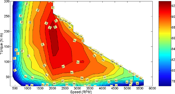
FIGURE F.1 2007 Camry Hybrid motor-inverter efficiency map.
SOURCE: Ricardo (2008).
F.1.4 A Potential Disruptive Change: Autonomous Vehicles
A possibility that could portend truly disruptive change in the LDV sector over the next few decades is the emergence of autonomous, self-driving vehicles. All major automakers, as well as transportation agencies in many countries, have research, development, and demonstration programs underway to explore intelligent transportation system (ITS) technologies. Implementing ITS is likely to require making substantial new infrastructure investments, facing the complexities of human factors and the man-machine interface, and working through numerous institutional issues about responsibility and liability for vehicles operating with varying degrees of autonomy. Nevertheless, it is likely that by mid-century some form of ITS technology will begin to reshape personal mobility.
The general concept involves cars that are still individually owned and operated but driven by computer rather than under direct human control. Although some autonomous vehicles might be part of publicly managed networks, the greatest potential for a paradigm shift is likely to involve autonomous cars that preserve the core appeal of personal mobility while freeing drivers of the time, attention, and skill required to navigate and operate vehicles themselves. Robot vehicles could be dispatched for goods movement and to securely transport non-drivers such as children, the disabled, or the elderly. Autonomous vehicles could drive on a “dumb” road infrastructure little different than today’s, but they might also evolve as part of an intelligent, energized road network. The U.S. Department of Transportation’s Research and Innovative Technology Administration (RITA) has several programs researching ITS options (DOT, 2011). The technologies involved offer the potential to dramatically improve safety, enhance mobility, and reduce congestion using strategies such as vehicle-to-vehicle (v2v) and vehicle-to-infrastructure (v2i) communications as well as robotic driving.
Autonomous vehicles are already in use on an experimental basis (Vanderbilt, 2012). At one end of the spectrum are robot vehicles having capabilities similar to today’s cars, such as the modified sport utility vehicles seen in autonomous vehicle competitions sponsored by the Defense Advanced Research Projects Agency (DARPA; Gibbs 2006). Google has been testing conventional cars with autonomous
driving apparatus on public roads (Markoff, 2010). At the other end of the spectrum are small, one-or two-person podcars such as the MIT Media Lab’s City Car prototypes, the General Motors Electric Networked-Vehicle (EN-V) concept, and similar ideas as discussed by Mitchell et al. (2010). Another example is Toyota’s Fun-Vii concept from the 2011 Tokyo motor show, featuring more bandwidth than horsepower capability and designed for automated driving on an intelligent road infrastructure. An emphasis on a virtual environment for drivers was anticipated by Ford’s concept 24-7 in 2000, and the future importance of ITS systems, including plausible timelines for implementation over the next two decades, was outlined in the “Blueprint for Mobility” announced by Bill Ford at the Mobile World Congress (Ford, 2012).
The committee did not attempt to quantify the possible impacts of autonomous cars. Not only are the characteristics of such vehicles highly uncertain, but also their effects on fuel use and GHG emissions are very difficult to project. By themselves, full-size robot vehicles (such as those of the DARPA challenge) might offer some modest efficiency gains, perhaps similar to those of optimized “ecodriving.” However, networked autonomous vehicles would offer enormous safety benefits, perhaps nearly eliminating collision risks, and so could foster greater acceptance of smaller vehicles with significantly lower energy demands. Such synergies might result in automobiles with fuel consumption rates a factor of two or more below those estimated in this study. Even more dramatic reductions could be seen with small pod cars, which could cut per-mile fuel use by an order of magnitude or more compared to today’s LDVs (Mitchell et al., 2010, Figure 9.18).
On the other hand, the new mobility opportunities opened up by autonomous driving could dramatically increase overall vehicle travel. For small and inexpensive robot cars, ownership and usage could rise as individuals, households, and businesses purchase multiple vehicles that might be simultaneously dispatched for numerous purposes, occupied or not. Large autonomous cars could make long trips more comfortable and enable their operators to do a wide variety of things—working, entertaining, eating, sleeping, and many other activities—when freed of the need to drive, fostering longer commutes and further dispersion of settlement. While the energy use and emissions per mile of travel might decrease, those gains could be swamped by a large increase in vehicle miles travelled. The range of possible outcomes for autonomous vehicles and how they might be used is far too vast to enable projection of their net impacts on petroleum demand and GHG emissions. Although such uncertainties preclude formal analysis, the committee recognizes that autonomous driving could well have a great transformative effect on the sector.
F.2 FUTURE VEHICLE COST AND EFFICIENCY ASSESSMENT
F.2.1 Overall Approach to Modeling
The energy required to move a vehicle is the energy delivered by the drive-train to the wheels plus the energy to operate the accessories. The drive-train energy provides multiple functions. At any instant:
EDT = EI + EHC + ERR + EAD + EA
where
| EDT | Energy delivered by the drivetrain to the vehicle wheels (total tractive energy) | |
| EI | Energy required to accelerate the vehicle, that is to overcome the inertia of the vehicle, which is made up of the vehicle mass plus the rotational inertia of tire/wheel/axle assemblies | |
| EHC | the energy required to provide hill-climbing | |
| ERR | Energy required to overcome the rolling resistance |
| EAD | Energy required to overcome the aerodynamic drag | |
| EA: | Energy provided by engine for accessories (air conditioner/heat pump, power steering, power brakes, water pump, alternator, oil pump) |
The energy available for overcoming inertia and hills determines the performance of the vehicle. Zero to 60 mph time in seconds quantifies vehicle acceleration. Gradeability, the grade at which a speed, often 65 mph, may be sustained, quantifies hill-climbing. The power-to-weight ratio determines both. Generally, acceptable acceleration assures acceptable hill-climbing, although this may not be the case in hybrid drivetrains with batteries that can provide power only in short bursts.
Over a driving cycle, which begins and ends at zero velocity and zero elevation change, net EI and EHC are zero, and
EDT = ERR + EAD + EA
The committee’s analytical approach is driven by two goals. First, it is highly important that this committee present its best assessment of 2050 technology potential. Second, the modeling is kept as simple as possible to focus on the important trends rather than the unpredictable details of vehicle technology in 2050.
Projections of future ICE efficiency have generally been done by assessing the benefits of different technology pieces. Major recent reports have done detailed assessments of a broad range of technologies to improve the efficiency of ICEs and transmissions and reduced vehicle loads (NRC, 2011)
These types of assessments work well up to about 2025 or perhaps 2030. However, their usefulness for 2050 suffers from two major problems. One is that it is impossible to predict what specific technologies will be used in 2050. The second is that as we push toward the boundaries of ICE efficiency, the synergies between different technologies becomes more and more important.
The approach chosen by the committee avoided these problems by modeling vehicle loads and powertrain efficiencies and losses. Engine efficiency was assessed based on thermodynamic and engineering principles. Layered on top of this were efficiency assessments of the transmission, electric powertrain components, and fuel cell stack, as well as vehicle load assessments and recovery of energy from braking and waste heat. This ensured that synergies would be properly assessed, and the modeled efficiency results would not violate basic principles. It also facilitated the extrapolation of input assumptions for 2050 vehicles.
The primary goal of the committee was to properly assess the relative efficiency of the different technologies. Thus, care was taken to use consistent assumptions across the different technologies. For example, the same vehicle load reduction assumptions (weight, aero, rolling resistance) were applied to all of the technology packages. Engine and transmission assumptions for the ICE case were used as the starting assumptions for HEV.
Six different vehicles were modeled, a Toyota Yaris, Toyota Camry, Chrysler 300C, Saturn Vue, Dodge Grand Caravan, and Ford F-150.
Meszler Engineering Services, under contract with the NRC for this study, developed a CAFE cycle energy audit model, layered with a loss model, to calculate miles per gallon (mpg) for future vehicles and technologies. The model does not calculate efficiency directly from the inputs; rather, baseline inputs were established that corresponded with specific baseline mpg values for each of the six vehicles. The model then calculates changes in miles per gallon based on changes in input assumptions over the federal test procedure and highway cycles.
Inputs to the model were developed by the NRC committee and were reviewed by expert external reviewers. Detailed inputs were developed for vehicles with four different technologies: ICE vehicles, HEVs, BEVs, and FCEVs. PHEV operation in charge depleting mode was assumed to match the efficiency of BEVs, and operation in charge sustaining mode was assumed to match the efficiency of
HEVs, so there was no modeling specific to PHEVs. Similarly, natural gas vehicles were assumed to have the same efficiency as other ICE engines.
Variables considered by the model (not all variables were used for each technology) are as follows:
• Vehicle load reductions, such as
—Vehicle weight,
—Aerodynamic drag,
—Tire rolling resistance, and
—Accessory load;
• ICE, such as
—Indicated (gross thermal) efficiency,
—Pumping losses,
—Engine friction losses,
—Engine braking losses, and
—Idle losses;
• Transmission efficiency;
• Torque converter efficiency;
• Electric drivetrain, such as
—Battery storage and discharge efficiencies,
—Electric motor and generator efficiencies, and
—Charger efficiency (BEV only);
• Fuel cell stack efficiency, such as
—Also the FCEV battery loop share of non-regenerative tractive energy;
• Fraction of braking energy recovered; and
• Fraction of combustion waste heat energy recovered.
The weight of the different technology packages was not adjusted to reflect the incremental weight of the technologies, such as the battery pack for BEVs. This was because the baseline efficiencies were matched to baseline vehicles, which included the incremental weight, weight reductions were input in terms of percentage weight reduction, and the battery pack sizes were scaled to efficiency improvements, implicitly scaling battery pack weight with other load reductions.
F.2.1.1 Development and Validation of Baseline Input Assumptions
Baseline inputs, including baseline mpg, for ICEs and HEVs were developed by the committee from energy audit data provided to the public by EPA, based upon computer simulation runs from Ricardo Engineering. EPA also provided public energy audit data based upon Ricardo’s computer simulation for advanced ICE and HEV technology packages. These advanced ICE and HEV technologies were representative of what Ricardo and EPA determined would be available by 2020 to 2025. However, it takes at least a decade to disseminate technology across the entire vehicle fleet, so the committee used these estimates as the 2030 midrange case. The 2010 baseline and 2030 midrange model inputs were developed directly from this Energy Audit data and fed through Meszler Engineering’s CAFE cycle energy audit model. The resulting mpg values were within 1 to 2 percent of the mpg results from the Ricardo simulation runs. Not only did this provide validation of the accuracy of the model, but these 2030 midrange inputs were used as the starting point for 2030 optimistic and 2050 input estimates.
The motor and battery efficiencies for BEVs and HEVs were assumed to be the same as for HEVs. The fraction of braking energy recovered was also assumed to be the same as developed for HEVs. The much larger battery packs used for PHEVs and BEVs should be able to capture higher rates of regenerative braking energy. On the other hand, a fully charged PHEV/BEV battery pack will have more limited headroom to capture high rates of regenerative braking energy. These were judged to be roughly offsetting factors.
Additional 2010 baseline input assumptions for BEVs and FCEVs were developed by Meszler Engineering Services based on public efficiency data for the Nissan Leaf, Honda Clarity, and Mercedes FCEV, including charger efficiency for BEVs and fuel cell efficiency and the battery loop share of non-regenerative tractive energy for FCEVs. These baseline inputs were developed to match public efficiency numbers for the Nissan, Honda, and Mercedes advanced vehicles and were validated by Meszler.
Development of input assumptions for the various 2030 and 2050 scenarios is described in the different technology sections, except for the 2030 midrange case for ICE and HEV, which was developed as described above. The attached Excel spreadsheet model, Appendix F Vehicle Input Spreadsheet, shows how the various vehicle characteristics were developed from the baseline.
F.2.1.2 Vehicle Cost Calculations
Costs are more difficult to assess than benefits. Every existing cost assessment is simply someone’s expert (or not so expert) opinion. The committee examined existing cost assessments for consistency and validity. Fully learned out, high-volume production costs were developed in this part of the analysis.
The primary goal was to treat the cost of each technology type as equitably as possible. Care was taken to match the cost assumptions to the efficiency input assumptions. Results from the efficiency model were used to scale the size of the ICE, electric motor, battery, and hydrogen and compressed natural gas (CNG) storage tanks (as applicable). Consistent assumptions of motor and battery costs were used for HEVs, PHEVs, BEVs, and FCEVs. HEV costs were calculated using ICE costs as the base. PHEV, BEV, and FCEV costs were calculated based on the HEV costs using inputs on battery, motor, and electronics size and cost, plus adjustments for ICE removal (BEV and FCEV), converter costs (BEV), fuel cell stack (FCEV), and gaseous storage tanks (FCEV and CNG).
Costs were calculated separately for cars and light trucks. Data from the six different vehicles analyzed for efficiency were combined, where necessary, using a simple average of the three different cars (Yaris, Camry, and 300) or three different light trucks (Vue, Caravan, and F-150). The simple averages were compared to sales-weighted average numbers from EPA’s 2010 Fuel Economy Trends Report, (EPA 2012) where averages were 6.4 percent higher than the simple average of the baseline cars and 6.9 percent higher than the simple average of the baseline light trucks. These differences will not have a significant impact on the results, especially since the offsets for the cars and light trucks were very similar.
Costs were calculated in an attached Excel spreadsheet, Appendix F Vehicle Cost Summary. Data that must be input by the user are coded in blue font. Data from other sources are in black font. These data can be modified if desired, but care should be taken, as these are generally input directly from baseline vehicle assumptions or outputs from the efficiency model. Calculations made by the spreadsheet are in red font.
This section discusses where the inputs to the spreadsheet came from and how the spreadsheet calculates costs from these inputs.
Load Reduction
The cost of lightweight materials, aerodynamic improvements, and reductions in tire rolling resistance were assumed to apply equally to all vehicles and technology types.
• User inputs:
—Maximum proportion of weight reduction (percent of baseline vehicle weight) from high strength steel (HSS), aluminum (which includes other currently available lightweight materials such as magnesium and composites), and carbon fiber (which is only used for the 2050 optimistic case). The total amount of weight reduction must be set to be equal to the amount used for the efficiency calculations.
—Cost of reducing a pound of weight, with separate inputs for HSS, aluminum, and carbon fiber.
—Cost of aero improvements
—Cost of tire rolling resistance improvements
• Other data:
—Baseline vehicle weight is the average of the loaded vehicle weight for the 3 different models of cars or light trucks.
• Calculations:
—Cost of each lightweight material is the % load reduction times the baseline vehicle weight times the $/pound cost.
—Total cost is the sum of the cost of each lightweight material and tire and aero costs.
Internal Combustion Engines
This is perhaps the most subjective cost estimate, as ICE technology includes a vast array of incremental engine, transmission, and drivetrain improvements. Past experience has shown that initial costs of new technologies can be high, but generally drop dramatically as packages of improvements are fully integrated over time.
Fortunately, this is also the least important cost estimate. This is because the cost spreadsheet is set up to assess the incremental cost of other technologies relative to future ICE costs. Penetration of alternative technologies into the fleet is impacted by the difference in efficiency and cost compared to future ICEs, which is not affected by the ICE cost estimates.
• User Inputs:
—Future ICE technology cost (including transmission and drivetrain)
—Stop/start system cost
—Downsized, turbocharging cost
—Waste heat recovery cost
—Cost credit ($ per % power reduction times number of cylinders) for downsized powertrain due to load reductions
• Other Data:
—Number of cylinders: Average of the 3 different baseline models of cars or light trucks
—Percent power reduction is taken from the output of the efficiency modeling
• Calculations:
—Total credit for ICE downsizing is the cost credit times the percent power reduction times the average number of cylinders.
—Total ICE cost = the sum of load reduction, ICE technology, stop/start, turbocharging, and waste heat recovery costs minus ICE credit for load reduction
HEV Costs
HEVs begin the strategy of differential costing. Costs specific to the hybrid system are added to ICE costs, and credits are subtracted to arrive at the hybrid cost increment versus ICE.
Battery, motor, and power electronics costs are treated consistently for all technology types by creating a sub-table of battery costs and motor+power electronics costs. These costs are applied consistently to all of the technology types, along with individual assessments of the battery and motor size requirements.
• User Inputs:
—Motor+power electronics cost ($/kW)
—Battery cost ($/kWh)
—Motor size as % of total propulsion power
—Battery power-to-energy ratio (kW/kWh)
• Other Data:
—Total propulsion power (kW) is taken from the output of the efficiency modeling
—Miscellaneous hybrid component costs and credits (assumed to be the same for all vehicles and scenarios):
-Control electronics cost: $150
-Wiring: $200
-Blended brake control: $100
-DC-DC converter: $75
-Integration of motor into transmission: $50
-ICE size reduction: $100 credit
-Elimination of starter/alternator: $100 credit
-Elimination of torque converter: $75 credit
• Calculations:
—Motor size = Total propulsion power times motor % of total propulsion power (kW)
—Battery size = Motor size divided by the battery power-to-energy ratio (kWh)
—Hybrid cost = (ICE cost minus stop/start cost) plus (motor size × motor cost) plus (battery size × battery cost) plus (control electronic + wiring + blended brake control + DC-DC converter + motor integration) minus credits (ICE size reduction and elimination of starter/alternator and torque converter)
PHEV Costs
PHEV costs continue the strategy of building upon previous cost estimates, in this case building upon the HEV cost estimates.
• User Inputs:
—Motor + power electronics cost ($/kW)
—Battery cost ($/kWh)
—Motor size as % of total propulsion power
—Battery depth-of-discharge (%)
—Electric drive range (miles) on test cycles (1.2 × desired real world range)
—On-board converter (for recharging) cost
—ICE downsizing credit (versus HEV ICE)
• Other Data:
—Total propulsion power (kW) is taken from the output of the efficiency modeling
—Energy consumption in electric-drive mode (kWh/mi) is taken from the output of the efficiency modeling.
• Calculations:
—Motor size = Total propulsion power times motor % of total propulsion power (kW)
—Battery size = BEV energy consumption times desired battery range divided by battery depth-of-discharge
—PHEV cost = (HEV cost minus waste heat recovery cost) plus (PHEV motor size × motor cost) minus (HEV motor size × motor cost) plus (PHEV battery size × PHEV battery cost) minus (HEV battery size × HEV battery cost) plus converter cost minus ICE credit for PHEV versus HEV
BEV Costs
BEV costs also build upon the HEV cost estimates.
• User Inputs:
—Motor+power electronics cost ($/kW)
—Motor size as % of total propulsion power (usually 100 percent)
—Battery cost ($/kWh)
—Battery depth-of-discharge (%)
—Electric drive range (miles) on test cycles (1.3 × desired real world range, including 10 percent reserve energy)
—On-board converter (for recharging) cost
—Credit for elimination of ICE
• Other Data:
—Total propulsion power (kW) is taken from the output of the efficiency modeling
—Energy consumption (kWh/mi) is taken from the output of the efficiency modeling.
• Calculations:
—Motor size = Total propulsion power times motor % of total propulsion power (kW)
—Battery size = Energy consumption times desired range divided by battery depth-of-discharge
—BEV cost = (HEV cost minus ICE tech, turbo, and waste heat recovery costs) plus (BEV motor size × motor cost) less (HEV motor size × motor cost) plus (BEV battery size × BEV battery cost) less (HEV battery size × HEV battery cost) plus converter cost minus credit for elimination of ICE plus ICE credit already accounted for in ICE and HEV cost estimates.
FCEV costs also build upon the HEV cost estimates.
• User Inputs:
—Motor+power electronics cost ($/kW)
—Battery cost ($/kWh)
—Motor size as % of total propulsion power (usually 100 percent)
—Fuel cell system size as % of total propulsion power
—Fuel cell system efficiency (%)
—Fuel cell system cost ($/kW)
—Battery depth-of-discharge (%)
—Battery driving range (miles) on test cycles (1.2 x desired real world range)
—Total vehicle driving range (miles) on test cycles (1.3 x desired real world range, including 10 percent reserve energy)
—H2 tank cost: fixed plus $/kg of hydrogen
—Credit for elimination of ICE
• Other Data:
—Total propulsion power (kW) is taken from the output of the efficiency modeling
—Energy consumption in electric-drive mode (kWh/mi) is taken from the output of the efficiency modeling.
—Overall vehicle hydrogen consumption (kWh/mi) is taken from the output of the efficiency modeling.
—Conversion factors for kWh of hydrogen to kg.
• Calculations:
—Motor size = Total propulsion power times motor % of total propulsion power (kW)
—Battery size = BEV energy consumption times desired battery range divided by battery depth-of-discharge
—Fuel cell system power = Total propulsion power times fuel cell system size as % of total propulsion power
—H2 storage (kg) = Vehicle H2 consumption rate converted to kg/mile times desired range
—FCEV cost = (HEV cost minus ICE tech, turbo, and waste heat recovery costs) plus (FCEV motor size × motor cost) less (HEV motor size × motor cost) plus (FCEV battery size × FCEV battery cost) less (HEV battery size × HEV battery cost) plus (fuel cell system power × $/kW) minus credit for elimination of ICE plus ICE credit already accounted for in ICE and HEV cost estimates plus fixed tank cost plus (variable tank cost × kg H2)
CNG Vehicle Costs (ICE and HEV)
CNG costs are assumed to be the same as gasoline ICE and HEV costs plus the cost of a CNG storage tank.
• User Inputs:
—Total vehicle driving range (miles) on test cycles (1.3 x desired real world range, including 10 percent reserve energy)
—CNG tank cost: fixed plus $/GGE of CNG
• Other Data:
—Overall vehicle GGE consumption (gal/mi) is taken from the output of the efficiency modeling of gasoline ICE and HEV vehicles
• Calculations:
—CNG storage (GGE) = Vehicle fuel consumption rate times the desired range
—CNG cost = (ICE or HEV cost) plus fixed tank cost plus (variable tank cost × GGE)
F.2.2 Energy Modeling Methodology8
F.2.2.1 Summary of Modeling Approach
All fuel economy (and, by extension, fuel consumption) estimates discussed in Chapter 2 or this Appendix, unless otherwise noted, are intended to represent the level of fuel economy that would be achieved under the CAFE testing regime. Such levels are generally higher than the level of fuel economy that would be expected during real-world vehicle operation, but are consistent with the level of fuel economy that vehicle manufacturers would be expected to achieve in response to U.S. regulatory requirements.9 The scenarios in Chapter 5 convert the test results to on-road fuel economy. The next section provides a brief overview of CAFE program procedures.
For this project, CAFE fuel economy was estimated using what can best be described as a two-step process. In the first step, the tractive energy required to navigate the CAFE driving cycles using a given vehicle is estimated. Tractive energy is the amount of energy that must be delivered to the wheels of a vehicle. Since CAFE testing involves defined driving cycles, and the inertial characteristics of the subject test vehicle can be measured, the energy required to navigate the driving cycles can be estimated using the fundamental physical properties of motion. While it is not the intent of this appendix to provide a detailed exposition of the associated physical properties (as these are published in any number of engineering dynamics textbooks and other reference sources), Section F.2.2.3 provides an overview of the basic properties associated with tractive energy estimation.
Once tractive energy requirements have been estimated, the second step of the modeling process involves “working backwards” from the wheels of a vehicle through the various energy transfer mechanisms (and their associated losses) to the vehicle engine (or primary energy source) to derive an associated energy input requirement (or, in more conventional terms, an input fueling rate).10 This energy input rate can then be readily converted into an equivalent fuel economy estimate using the volumetric energy content of the associated fuel (e.g., gasoline) and the distance travelled (or, more accurately,
_____________________________
8 Section F.2.2 was provided by Dan Meszler, Meszler Engineering Services.
9 CAFE fuel economy is generally higher than that achieved in real-world operation for several reasons, but primarily due to the fact that the driving cycles associated with CAFE testing are less demanding than those typically encountered in everyday driving and the fact that not all vehicle accessories (e.g., air conditioning systems) are operational during CAFE testing. For this reason, the fuel economy of vehicles that is published for consumer use is adjusted downward from the levels associated with the CAFE program.
10 For a conventional internal combustion engine vehicle, the energy transfer path would proceed from the wheels through the differential, transmission, and torque converter (if present) to the flywheel. Internal engine losses associated with friction, pumping, braking (engine braking), and accessories (those that are operational during the CAFE cycles) are then accounted for to derive an estimate for the gross thermal energy available through fuel combustion. The associated input energy requirement to the engine is then estimated by applying a cycle average gross thermal (i.e., indicated) efficiency to the estimated gross thermal energy. For HEVs, an e-machine (motor/generator, controller, and enhanced battery) and its associated losses are integrated into the energy transfer path. For BEVs, the engine losses are removed and battery charger losses are added. For FCEVs, the battery charger is removed and a fuel cell system is added into the BEV energy transfer path.
simulated) over the driving cycle. Below is additional information related to this energy loss accounting as well as information on how baseline values for the various losses were estimated and validated.
The strengths and weaknesses of this two-step approach, relative to other commonly used approaches to fuel economy estimation, should be recognized. The approach employed herein is generally superior to estimation methods based on individual technology impacts or so-called lumped parameter (combined technology impact) approaches, because it explicitly limits the fuel economy improvements of “overlapping” technologies (i.e., technologies that target the same energy loss mechanism). Once losses are reduced for any given loss mechanism, those losses are not “available” for reduction to any additional technology. For example, once pumping losses go to zero, it is physically impossible to generate additional fuel economy improvements through another pumping loss reduction technology.11 The price to be paid for this constraint is that the model user must estimate energy impacts on a loss-specific basis as opposed to the more straightforward technology basis of the alternative approaches. Model inputs are not based explicitly on the introduction of technology, but on the effects of that new technology on specific energy losses—effects that must be explicitly defined by the model user.
The two-step approach employed herein is generally less sophisticated than detailed simulation modeling, which involves defining the physical and operational characteristics of the various energy transfer processes that constitute a vehicle powertrain and then modeling energy transfer from fuel input to energy output (at the vehicle wheels). The two-step approach can be viewed as essentially a summarization of the simulation modeling process, wherein the various loss mechanisms that would be quantified through a detailed simulation model are converted to aggregate energy loss inputs for the two-step model. In effect, the two-step model, given energy loss inputs derived from a detailed simulation model, would generate the same fuel economy estimates as the simulation model. This, in fact, is the procedure that is generally used to validate the baseline fuel economy estimates from the two-step model. However, whereas the detailed simulation model would explicitly account for the effects of any new technology added to a vehicle (given an accurately developed module defining the characteristics of that technology), the two-step model accounts for the effects of that same technology through a user input estimate of the technology’s effects on one or more energy loss mechanisms. Both the simulation model and the two-step model include an explicit estimation of tractive energy impacts due to changes in vehicle road load characteristics.
As is the case with actual CAFE compliance, CAFE fuel economy is estimated as the weighted average of energy (and fuel) consumption across the two driving cycles that comprise CAFE testing. The “city cycle” (i.e., the Federal Test Procedure) contributes 55 percent of overall CAFE energy requirements, while the “highway cycle” (i.e., the Highway Fuel Economy Test) contributes the remaining 45 percent. As with CAFE compliance, energy impacts associated with vehicle accessories that are not engaged during CAFE testing (e.g., air conditioning) are not captured. Independent energy consumption adjustments for these “off-cycle” loads can be calculated, but they have not been estimated explicitly through the two-step modeling approach for this project. If such adjustments are presented, the associated estimation methodology is described outside of this appendix.
In addition to the basic CAFE cycle energy analysis, the modeling work for this project also includes tractive energy evaluation over a constructed “performance cycle.” The performance cycle is essentially a manufactured cycle designed to estimate the peak power required to achieve published 0-60 acceleration times for the evaluated vehicles. Tractive energy requirements are estimated over the performance cycle in exactly the same manner as described above (and detailed below) for the CAFE cycles. Estimated tractive energy required during each second of the performance cycle is equivalent to the power required during that second.12 The maximum power estimated over the performance cycle is an indicator of the peak power required at the wheels. Peak power at the wheels is then converted into peak
_____________________________
11 Of course, it is not expected that pumping losses will go to zero (except for engineless BEVs and FCEVs); the premise is simply easiest to understand through a zero loss description.
12 For example, power (P) in watts is equal to energy (E) in newton-meters per unit time in seconds. If we evaluate energy requirements at a frequency of 1 hertz (i.e., once per second), then P = (E / seconds) × 1 second = E.
required engine (or alternative energy source) power in exactly the same manner as described above (and detailed below) for the “second step” of the CAFE fuel economy modeling process employed for this project. This allows for a reasonable estimation of the engine (or alternative power source) peak output required to achieve the same level of vehicle performance as observed for baseline ICE vehicles. The final section of this appendix provides an expanded discussion of this peak power requirement estimation process.
F.2.2.2 Summary of CAFE Procedures13
CAFE testing consists of two driving cycles, one nominally intended to represent city driving and one nominally intended to represent highway driving. The ability of either cycle to accurately reflect current driving behavior is limited, and for this reason the advertised fuel economy of a vehicle is based on both CAFE and supplemental testing, but CAFE compliance is limited to these two driving cycles alone. This allows for both standardized testing and a consistent historic record, with the realization that CAFE fuel economy will be 20-30 percent higher (nominally) than actual real-world fuel economy.
The city portion of the CAFE test is based on a driving cycle known as the Urban Dynamometer Driving Schedule (UDDS). Figure F.2 graphically depicts the UDDS. City cycle testing is actually based on one complete run of the UDDS, followed by a 10 minute engine-off period, followed by a repetition of the first 505 seconds of the UDDS. For this reason, the UDDS is generally split into two components. The first 505 seconds of the cycle are known as Bag 1, with the remaining 864 seconds of the cycle known as Bag 2. The subsequent repetition of the first 505 seconds of the cycle is known as Bag 3. The “bag” terminology is derived from the fact that emissions are collected in three separate polyvinyl fluoride bags, one for each of the three portions of the cycle. In total, this three-bag cycle is known as the Federal Test Procedure. Table F.10 presents summary statistics for the UDDS, the FTP, and the component FTP bags.
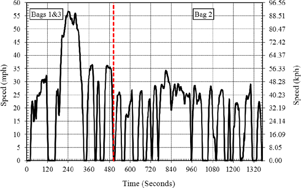
FIGURE F.2 Urban dynamometer driving schedule.
SOURCE: See http://www.epa.gov/otaq/standards/light-duty/udds.htm.
_____________________________
13 This section is intended only to provide an overview of CAFE procedures. Readers interested in further detail are referred to Title 49 Parts 523-538, Title 40 Parts 86 and 600, and Title 10 Part 474 of the Code of Federal Regulations that, in combination, define the various regulatory requirements associated with the CAFE program.
TABLE F.10 CAFE Driving Cycle Statistics
| Cycle Metric | Units | Complete UDDS | FTP Bags 1&3 | FTP Bag 2 | Complete FTP | Complete HwFET | |||
| Cycle duration | sec | 1369 | 505 | 864 | 1874 | 765 | |||
| Cycle duration | min | 22.82 | 8.42 | 14.40 | 31.23 | 12.75 | |||
| Cycle distance | miles | 7.4504 | 3.5910 | 3.8594 | 11.0414 | 10.2567 | |||
| Cycle average speed | mph | 19.59 | 25.60 | 16.08 | 21.21 | 48.27 | |||
| Cycle maximum speed | mph | 56.70 | 56.70 | 34.30 | 56.70 | 59.90 | |||
| Cycle average acceleration | mph/sec | 0.897 | 0.913 | 0.888 | 0.901 | 0.384 | |||
| Cycle maximum acceleration | mph/sec | 3.30 | 3.30 | 3.30 | 3.30 | 3.20 | |||
| Cycle maximum deceleration | mph/sec | –3.30 | –3.30 | –3.30 | –3.30 | –3.30 | |||
| Cycle idle time | sec | 241.0 | 94.0 | 147.0 | 335.0 | 4.0 | |||
| Cycle idle time | min | 4.02 | 1.57 | 2.45 | 5.58 | 0.07 | |||
| Fraction of cycle time at idle | 17.6% | 18.6% | 17.0% | 17.9% | 0.5% | ||||
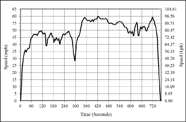
FIGURE F.3 Highway fuel economy test driving cycle.
SOURCE: See http://www.fueleconomy.gov/feg/fe_test_schedules.shtml.
The highway portion of the CAFE test is based on a driving cycle known as the Highway Fuel Economy Test (HwFET). Figure F.3 graphically depicts the HwFET. Unlike the city cycle, the highway test is run in its entirety without stop. Compared to the city cycle, the highway cycle is of generally higher speed with less transient operation. Table F.10 presents summary statistics for the HwFET.
As indicated above, CAFE is based on a 55/45 weighting of the city and highway test results. Average city cycle fuel consumption (gallons per mile, the inverse of fuel economy) is multiplied by 0.55,
while average highway cycle fuel consumption is multiplied by 0.45. The results of these two operations are summed and CAFE fuel economy is equal to the inverse of the sum.
F.2.2.3 Tractive Energy Estimation
As described above, the first step in the two-step modeling approach consists of the estimation of the tractive energy required by a specific vehicle to navigate the CAFE driving cycles. For a given set of vehicle characteristics and a specified driving cycle, the tractive energy required to navigate the driving cycle is defined precisely by physics and can thus be calculated accurately (without actually testing the vehicle). Similar calculations underlie both the more detailed vehicle simulation models and the less detailed two-step model employed in this project. Given the myriad references that describe the physical theory underlying the required calculations, it is not the intent of this report to provide a robust description of either the underlying principles or the required calculations.14 Nevertheless, a brief overview follows of the basic issues that are considered in the tractive energy calculations, as implemented in the two-step model used for this project.
To avoid any confusion with subsequent (second step) energy loss calculations, it is easiest, for tractive energy calculation purposes, to visualize the vehicle as freed of its power source and all related energy transfer technology (i.e., it is without an engine and drivetrain or other source of energy), so that its wheels are free to roll, and those wheels are themselves subject to no frictional losses in their attachment to the vehicle. Tractive energy is then the energy that must be supplied to navigate this powerless vehicle over a given driving cycle, in this case, the CAFE driving cycles described above. Since these test cycles are conducted indoors using a stationary vehicle, forces related to wind, cornering, and grade are fixed at zero.15
Under such conditions, the forces acting on a vehicle as it navigates a defined driving cycle are related to three influences: (1) tire rolling resistance, (2) aerodynamic drag, and (3) required vehicle motion. Tire rolling resistance is a measure of the force that must be applied to overcome the deformation characteristics of a tire (i.e., the force required to make the tire roll rather than deform). Aerodynamic drag is a measure of the force that must be applied to overcome the frictional characteristics of air (i.e., air has mass and thus induces a force that opposes vehicle motion). Vehicle motive force is a measure of the force required to induce a specified acceleration (or deceleration, which is simply a negative acceleration). Together, these three influences define the net force that must be applied to a vehicle to navigate a defined driving cycle. In mathematical terms:
F = R + D + M
where
F = the net force required to move the vehicle,
R = the force of rolling resistance,
_____________________________
14 Readers interested in detailed expositions on vehicle dynamics (which underlie the calculation of tractive energy) can consult any of a large number of available texts and reference papers. Although by no means meant to imply primacy amongst such references, examples include the following: Thomas D. Gillespie, Fundamentals of Vehicle Dynamics, ISBN 1-56091-199-9, Society of Automotive Engineers, Inc., Warrendale, Pa., March 1992. Robert Bosch GmbH, Automotive Handbook, 4th Edition, Stuttgart, Germany, October 1996. Gino Sovran and Mark S. Bohn, General Motors Research Laboratories, “Formulae for the Tractive-Energy Requirements of Vehicles Driving the EPA Schedules,” Technical Paper 810184, ISSN 0148-7191, Society of Automotive Engineers, Inc., Warrendale, Pa., 1981.
15 Vehicle motion is simulated using a chassis dynamometer (a set of, usually floor-mounted, rollers that rotate to absorb the motion that would otherwise be imparted by a set of spinning wheels) and appropriate load settings.
D = the aerodynamic drag force, and
M = the required motive force.
Rolling resistance is primarily related to the design characteristics of the vehicle tires and vehicle mass. It is generally represented as:
R = (r0 + r1v + r2v2) × mg
where
r0, r1, r2 = tire rolling resistance coefficients,
v = vehicle velocity,
m = vehicle mass, and
g = gravitational acceleration (9.80665 meters per second squared).16
The three rolling resistance coefficients measure the design resistance of the tire. For radial tires, the velocity squared coefficient (r2) is generally negligible and is usually ignored (as is the case for this project). The velocity coefficient (r1) is generally numerically small relative to r0, but can have a significant effect on overall rolling resistance as velocity increases.
Aerodynamic drag is primarily related to the airflow characteristics and frontal cross sectional area of the vehicle. It is generally represented as:
D = Cd × A × 0.5 × v2 × ρ
where
Cd = the coefficient of drag of the vehicle,
A = the frontal area of the vehicle,
v = vehicle velocity, and
ρ = air density (1.2041 kilograms per cubic meter).17
The coefficient of drag can range from as low as 0.15 for an optimally streamlined vehicle to as high as 0.7 for an open convertible passenger car to more than 1 for large freight trucks. Almost all passenger cars and light trucks have coefficients in the range of 0.25-0.45. The frontal area of a vehicle represents a two-dimensional profile of the air that must be moved out of the way for the vehicle to pass. It essentially is defined by the area that is perpendicular to the line of sight of a person looking directly at an oncoming vehicle and includes the cross sectional area of protuberances such as tires, mirrors, etc. Although the precise frontal area must be measured for any given vehicle, most generally fall within a range of 80-85 percent of the product of a vehicle’s geometric width and height.
The motive force is primarily related to the mass of the vehicle and the acceleration required to navigate the specified driving cycle. It is generally represented as:
F = m × a = m × (xΔv/Δt)
_____________________________
16 Gravitational acceleration varies with one’s position on the Earth, with values generally ranging from 9.78-9.82 meters per second squared. The value used for this project is the officially established value for standard gravity as set by the 3rd General Conference on Weights and Measures in 1901.
17 Air density is influenced by ambient temperature and ambient pressure/elevation. The value presented here (and used for this project) is for standard conditions of 101.33 kilopascals and 20°C (68°F), as prescribed for constant volume sampler calibration in 40 CFR Part 86, Subpart N, §1319-90.
where
m = vehicle mass,
a = vehicle acceleration,
Δv = change in vehicle velocity, and
Δt = associated time interval.
More precisely, the change in velocity over the change in time would be expressed as the derivative dv/dt to signify the properly instantaneous nature of the force calculation. However, actual tractive energy calculations are always performed over some discrete time interval. In the case of this project, that interval is 1 second, so that the force calculations are performed once for each driving cycle second, or 1,874 times for the FTP cycle and 765 times for the HwFET cycle.
Finer resolutions are possible and are routinely employed in simulation models, but typical driving cycles (including the CAFE cycles evaluated in this study) are themselves only defined at a resolution of 1 second. Finer resolutions enable the more precise simulation of non-linear powertrain effects, but such effects are not relevant to tractive energy calculations (which are powertrain independent). Tractive energy requirements are sensitive to driver behavior, both in terms of the driver’s ability to adhere to the driving cycle and in terms of driving behavior between defined cycle seconds, but fuel economy testing allows for only minor deviations from driving cycle speed/time definitions.
Simulation models that include a driver module (to emulate human response to driving cycle requirements) might derive more robust tractive energy requirements than the 1-hertz model employed for this project, but any increase in precision is only as “good” as the driver module itself, and the magnitude of any deviations should be minor by definition. For comparative purposes, the tractive energy requirements calculated for the six vehicle platforms evaluated in this project (see below for a description of the six platforms) were compared to corresponding tractive energy requirements predicted by a high resolution vehicle simulation model. All six tractive energy calculations agreed to within ±3 percent, and all were ultimately calibrated to agree to within ±0.05 percent so that any predicted changes in tractive energy requirements (due to forecasted changes in vehicle load parameters) are expected to be quite accurate.18
The use of vehicle mass in the motive force equation is also somewhat imprecise, because each tire also possesses rotational inertia that must be overcome to induce motion. The mass equivalent of this rotational inertia (for a single tire) is calculated as:
mrot = I / (rr2)
where
mrot = rotational inertia equivalent mass,
I = tire rotational inertia, and
rr = tire rolling radius.
The equivalent mass imparted by four tires is four times mrot, so that the total mass associated with the motive force is m + 4 mrot, and the overall motive force is:
F = (m + 4 mrot) × (Δv/Δt)
_____________________________
18 Although not investigated completely due to limitations in the type of data available for the simulation modeling runs, it is believed that the magnitude of the tractive energy deviations is more dependent on differences in the assumed vehicle load parameters for each of the six vehicle platforms than on any difference in the tractive energy calculations themselves.
It is this more precise definition that is applied for this project, although the difference between the less and more precise definitions is generally minor, as the mass due to rotational inertia is small compared to typical vehicle mass (typically less than 3 percent and smaller still for high mass vehicles). Nevertheless, this relationship can vary, especially if mass reduction technology is employed in an aggressive fashion, so the more precise rotational effects are considered.
As indicated, the net force required to navigate a specified driving cycle is dependent on several vehicle characteristics—namely, the tire rolling resistance coefficients, vehicle mass, the vehicle coefficient of drag, vehicle frontal area, tire rotational inertia, and tire rolling radius—and several parameters associated with the specified driving cycle—namely, velocity and acceleration per unit time. These latter parameters are defined by the driving cycle itself, and for this project represent the characteristics of the two CAFE driving cycles as depicted above. Table F.11 presents the former vehicle-specific parameters (under baseline conditions) that have been assumed for this project.
Tractive energy is the energy expended in exerting the force required to navigate a driving cycle over the distance associated with that cycle. Since driving cycles are generally defined in terms of velocity and time (rather than distance), it is convenient to express distance in terms of velocity and time (as distance = velocity × time) and tractive energy as:
TE = F × s = F × v × t
where
F = the net force required to move the vehicle,
s = the distance over which the force is applied,
t = the time interval over which the force is applied, and
v = vehicle velocity over the time interval.
As with the force calculation, the precise energy calculation would be expressed as the instantaneous energy required for a given instantaneous force and time. Total tractive energy is then the sum (or integration) of this instantaneous energy over an entire specified driving cycle. In keeping with the 1 hertz nature of the force calculations, the energy calculations for this project are also performed once per second and summed over the driving cycle to obtain the total estimated tractive energy required to navigate the cycle.
This estimated tractive energy is the amount of energy that must be available at the vehicle’s wheels. Given this value, it is possible to “work backwards” from the wheels through a vehicle’s drivetrain and engine (or alternative energy source) to derive the required amount of energy that must be input into the engine (or alternative energy source). This “path backwards” represents the second step of the two-step modeling process, as described in more detail below. Once the required input energy is “known” (i.e., estimated), it is a simple arithmetic exercise to convert input energy into fuel economy (which is essentially energy per unit distance, with the latter being defined by the specific driving cycle evaluated).
Although not critical to determining overall input energy requirements, there are a few component calculations inherent in the tractive energy estimation process that are helpful in the estimation of certain energy transfer inputs used in the second step of the modeling process. Therefore, these calculations are discussed briefly here. Such calculations are also useful in understanding the tractive energy impacts of changes in vehicle load characteristics (e.g., rolling resistance, aerodynamic drag, vehicle mass).
TABLE F.11 Baseline Vehicle Tractive Energy Parameters
| Parameter | Units | Toyota Yaris | Toyota Camry | Chrysler 300 | Saturn Vue | Grand Caravan | Ford F-150 | ||
| r0 coefficient | 0.009402 | 0.008223 | 0.011288 | 0.006913 | 0.007207 | 0.008245 | |||
| r1 coefficient | sec/m | 2.36E-05 | 4.24E-06 | 4.99E-05 | 0.000181 | 0.000165 | 0.000111 | ||
| r2 coefficient | sec2/m2 | 0 | 0 | 0 | 0 | 0 | 0 | ||
| Cd coefficient | 0.32 | 0.30 | 0.33 | 0.37 | 0.34 | 0.41 | |||
| Frontal area | ft2 | 24.76 | 24.76 | 25.83 | 26.91 | 30.14 | 35.20 | ||
| Frontal area | m2 | 2.30 | 2.30 | 2.40 | 2.50 | 2.80 | 3.27 | ||
| Vehicle mass | pounds | 2,625 | 3,625 | 4,000 | 4,000 | 4,500 | 6,000 | ||
| Vehicle mass | kg | 1,190.7 | 1,644.3 | 1,814.4 | 1,814.4 | 2,041.2 | 2,721.6 | ||
| Rolling radiusa | m | 0.282 | 0.320 | 0.342 | 0.340 | 0.330 | 0.382 | ||
| Rotational inertiaa | kg-m2 | 0.56 | 0.90 | 0.97 | 0.95 | 0.94 | 1.00 | ||
| Rotational massb | kg | 28.17 | 35.16 | 33.17 | 32.87 | 34.53 | 27.41 | ||
| Effective mass | kg | 1218.9 | 1679.4 | 1847.6 | 1847.3 | 2075.7 | 2749.0 | ||
| Rotational mass factor | 1.024 | 1.021 | 1.018 | 1.018 | 1.017 | 1.010 | |||
a Per tire.
b Total for four tires.
Any given driving cycle can be summarized in terms of three basic energy modes: (1) an energy input mode, during which tractive energy must be supplied to meet the velocity requirements of the cycle, (2) an energy output (or dissipative) mode, during which tractive energy must be removed to meet the velocity requirements of the cycle, and (3) a zero energy mode, during which tractive energy is neither supplied or removed. The zero energy mode basically occurs when a vehicle is idling during the periods of a driving cycle where the demanded velocity is zero.19
Energy input modes occur during the acceleration and cruise (constant velocity) portions of a driving cycle, wherein tractive energy must be supplied to overcome opposing road load forces and, in the case of acceleration, to supply the required motive force.20 Energy input is also required during vehicle deceleration events in which road load forces are sufficiently large so that inertial momentum is not sufficient to maintain the velocity required by the driving cycle without additional energy input. Such powered deceleration events are not uncommon (throttle is reduced, but not closed).
Energy output modes occur during decelerations in which road load forces are not large enough to slow the vehicle as rapidly as the driving cycle demands. Some form of braking must occur during such
_____________________________
19 It is also possible that a vehicle may encounter a brief zero energy demand condition during a deceleration in which road load forces are exactly offset by unpowered inertial momentum. Such encounters are both rare (since the driving cycle deceleration profile must exactly balance the encountered road load forces) and vehicle specific (since the inertial and road load forces of one vehicle are unlikely to exactly match those of another). Such non-idle zero energy modes are not the same as closed throttle “coasting” events, but rather constitute a very small subset of such events, wherein the small amount of motive energy provided at closed throttle is exactly balanced by opposing road load forces plus inertial deceleration forces. In the vast majority of closed throttle “coasting” events, these forces will not be in balance and “engine” braking (an energy output mode) will occur. Closed throttle coasting is not typically a zero energy mode.
20 Road load forces are defined as the sum of rolling resistance and aerodynamic drag forces, signifying those forces that arise independent of the specific motive force demands of a driving cycle.
modes so that tractive energy is removed faster than can be accomplished through the combination of inertial and road load forces. This braking can be limited to engine braking in instances where drivetrain inertia is sufficiently large to impart the necessary deceleration, or involve wheel-based friction braking in instances where additional tractive energy must be removed to impart the required deceleration.
During tractive energy analysis, each component of a driving cycle (meaning, in the case of this project, each second of the driving cycle) is determined to be in one of these energy modes, so that when integrated across the entire cycle, the energy input and output fractions are clearly identifiable, as are the individual motive, rolling resistance, and aerodynamic drag-induced components of those fractions. One consequence of this is that the fraction of tractive energy that is dissipated through braking is quantified. This fraction, in combination with the overall tractive energy estimate, dictates the maximum amount tractive energy that can be recovered through regenerative braking technology. Properly applying this maximum recovery fraction to regenerative braking calculations associated with this project ensures that such calculations are properly bounded and do not inherently overestimate potential braking energy recovery.
A second, less obvious, consequence of the detailed tractive energy analysis is that the effects of changes in specific vehicle load parameters, as well as their interactions, can be fully understood. Although such effects are generally considered to be intuitively obvious, that is not always the case, and, additionally, synergistic effects can be masked without a detailed understanding of the various tractive energy modes.
Since, as shown above, the total tractive force (F) is equal to the arithmetic sum of the rolling resistance (R), aerodynamic drag (D), and motive (M) forces, the impacts on these three component forces (and their associated energies) are also additive. In other words, changes to vehicle load parameters generally impart non-overlapping influences on the energy required to move the vehicle.21 For example, reducing the rolling resistance force does not diminish the potential force reduction that can be achieved through reductions in the aerodynamic drag force. The forces are not multiplicatively related, as is the case for many technology implementations.22 This additive relationship has a few subtle effects that must be understood to fully appreciate tractive energy impacts.
It is desirable to be able to develop generalized relationships between a change in individual load parameters and the impact of that change on overall tractive energy (e.g., if rolling resistance is reduced by X percent, tractive energy requirements are reduced by Y percent). It is similarly desirable to be able to develop a generalized estimate of the tractive energy impact of changes in multiple load parameters. Unfortunately, the additive nature of the tractive force components renders such relations inherently imprecise. That is not to say that rules-of-thumb cannot be developed or that precise measures cannot be developed for a given set of vehicle characteristics, it is simply that precision is dependent on such characteristics, and, therefore, the precise relationships are inherently vehicle-specific.
_____________________________
21 There is an exception to this in the case of changes to vehicle mass (which affects both rolling resistance and motive force), and this is considered fully in the discussion that follows. However, for the introductory purpose of distinguishing the additive nature of vehicle load impacts, in contrast to an alternative multiplicative relationship wherein individual absolute impacts are dependent on implementation order, it is convenient to ignore the fact that changing mass affects both the motive and rolling resistance load parameters.
22 Take, for example, two technologies that improve vehicle driveline efficiency, say, through reductions in torque converter and transmission losses. In this case, the individual improvements target the same overall driveline losses, and once the efficiency of the torque converter is improved, the driveline losses available for reduction through transmission improvements are smaller than they would have been in the absence of the torque converter improvements. In effect, the absolute magnitude of the energy loss reductions associated with the installation the improved transmission are smaller if that transmission is installed with the improved torque converter than without. In this case, the improvements are multiplicatively related (i.e., their individual impacts cannot be arithmetically summed). This is true of any improvements that target the same energy losses, be those losses in the driveline, in the engine (e.g., pumping or friction losses), or anywhere else in the chain of processes that convert fuel energy to tractive energy.
The independence of individual tractive force components and the vehicle-dependent nature of the impact of changes to the individual tractive force components on the total tractive force (and, thus, on total required tractive energy) is perhaps most understandable mathematically. As discussed above, the tractive force relationship is:
F = R + D + M
If we implement a reduction of 40 percent in the rolling resistance force component, the new total tractive force becomes:
Fnew = (0.6 × R) + D + M
and the impact on the total tractive force is:
(Fnew/F) = [(0.6 × R) + D + M] / [R + D + M]
In the absence of knowledge of the relationship between the rolling resistance (R), aerodynamic drag (D), and motive (M) forces, it is simply not possible to derive a precise numerical estimate for the change in the total tractive force (Fnew/F). And, since the relationship between R, D, and M is vehicle dependent, the change in the total tractive force (Fnew/F) is also vehicle dependent. The only exception to this is the constrained case where the identical reduction is applied to all three force components. In this case, the new total tractive force becomes:
Fnew = (X × R) + (X × D) + (X × M) = X × (R + D + M)
where
X = 1 minus the percent reduction in force.
and the impact on the total tractive force is:
(Fnew/F) = [X × (R + D + M)] / [R + D + M] = X
So that the resulting reduction in the total tractive force is identical to that of the component forces.
Since the component forces are vehicle specific, it is perhaps informative to look at example impacts for a single vehicle. Suppose that vehicle has a tractive energy relationship as follows (in F = R + D + M format):
2.032793709 = 0.517590608 + 0.644968344 + 0.870234757
In this case:
R/F = 0.517590608 / 2.032793709 = 25.462%,
D/F = 0.644968344 / 2.032793709 = 31.728%
M/F = 0.870234757 / 2.032793709 = 42.810%
Based on these relationships, a 40 percent reduction in the rolling resistance force component can now be translated into a total tractive force impact as follows:
(Fnew/F) = [(0.6 × R) + D + M] / F = (0.6 × R/F) + D/F + M/F
(Fnew/F) = (0.6 × 0.25462) + 0.31728 + 0.42810 = 0.898152
So, a 40 percent reduction in the rolling resistance force results in a 10.2 percent reduction in total tractive energy (or a 2.5 percent total tractive force reduction per 10 percent reduction in rolling resistance force). We can, of course, apply the same 40 percent component force reduction to the aerodynamic drag and motive force components individually and derive the following:
(Fnew/F) = 0.25462 + (0.6 × 0.31728) + 0.42810 = 0.873088
(Fnew/F) = 0.25462 + 0.31728 + (0.6 × 0.42810) = 0.828760
and derive a 3.2 percent total tractive force reduction per 10 percent reduction in aerodynamic drag and a 4.3 percent total tractive force reduction per 10 percent reduction in motive force. However, this latter motive force reduction is misleading for two reasons. First, the driver of the motive force reduction is an underlying change in vehicle mass (since the acceleration component of the force is fixed by the driving cycle). Since mass affects both the motive and rolling resistance forces, a change in vehicle mass cannot affect the motive force alone. Second, a 40 percent reduction in motive force is not equivalent to a 40 percent reduction in vehicle mass due to the small mass influence of tire rotational inertia. If we instead specify the motive force reduction in terms of a 40 percent reduction in vehicle mass, the equivalent overall (vehicle plus rotational inertia) mass reduction is 39.16 percent (for this example). If we plug these complete mass impacts into the tractive force equations, we get:
(Fnew/F) = (0.6 × 0.25462) + 0.31728 + (0.6084 × 0.42810) = 0.730508
which equates to a 6.7 percent total tractive force reduction per 10 percent reduction in vehicle mass. To reiterate, however, these relationships are vehicle specific and will vary in accordance with the relative relationships between the rolling resistance, aerodynamic drag, and motive forces for any given vehicle.
A less significant, but nonetheless confounding, influence on the relationship between the total tractive force and changes in the three force components, results from the impact that changes in the individual components have on the relationship between powered (energy input) and braking (energy output) deceleration. The amount of powered versus braking deceleration for a vehicle (over a specified driving cycle) is determined by the sum of the three force components relative to driving cycle requirements. Changing one or more of the force components can affect the amount of powered deceleration, which induces a secondary effect on total tractive energy that leads to some (generally minor) variation from the arithmetically derived effects estimated above.
Take for example, a reduction in vehicle mass without any change in vehicle rolling resistance or aerodynamic drag parameters (except for the effect that changing mass itself has on rolling resistance). During high-speed decelerations, aerodynamic drag dominates road load forces, and since it is unaffected by the change in vehicle mass, it leads to a larger net deceleration force (since inertial momentum forces have decreased) for the reduced mass vehicle (as compared to the same vehicle at its original mass). This results in a shift in the deceleration energy modes (again relative to the mode fractions for the vehicle at its original mass) away from braking (energy out) deceleration and toward powered (energy in) deceleration. The net motive energy actually declines by an amount larger than the mass reduction would imply, since motive force is negative during these “added” powered decelerations, but this is offset by increases in the rolling resistance and aerodynamic drag energy associated with the “added” powered decelerations.23 The net effect on total tractive energy is minor (generally less than 1 percent), but, nonetheless, affects the otherwise straightforward arithmetic estimation process.
For example, if we compare the tractive energy for the same vehicle used in the arithmetic example above, we find that a 40 percent reduction in vehicle mass (a net mass reduction of 39.16 percent) with no additional rolling resistance or aerodynamic drag influences decreases motive force by 43.3 percent, as compared to an expectation of 39.16 percent in the absence of any shift in powered
23 In the case of rolling resistance, the increase is relative to the tractive energy that would be expected after the change in vehicle mass is applied, not relative to a pre-mass reduction baseline.
deceleration requirements.24 This is offset by 3.4 and 3.7 percent increases in rolling resistance and aerodynamic drag energy requirements, respectively, as compared to the energy that would be required in the absence of any shift in powered deceleration requirements. The net effect on total tractive energy is only about 0.1 percent (as compared to the nominal effect that would be expected in the absence of any shift in powered deceleration requirements).
Exactly the opposite occurs for changes in rolling resistance or aerodynamic drag without any change in vehicle mass. In both cases, reduced road load forces shift deceleration toward more braking. This eliminates some of the negative motive energy that accrues during powered decelerations, thus increasing motive energy (by 2.8 and 4.5 percent, respectively, for a 40 percent reduction in rolling resistance and aerodynamic drag forces).25 For the rolling resistance reduction, this is offset by 2.5 and 2.3 percent decreases in rolling resistance and aerodynamic drag energy requirements, respectively, as compared to the energy that would be required in the absence of any shift in powered deceleration requirements. The aerodynamic drag reduction induces corresponding changes of 3.5 and 4.5 percent. The net effect on total tractive energy is only about 0.1 and 0.2 percent, respectively, for the rolling resistance and aerodynamic drag changes (as compared to the nominal effect that would be expected in the absence of any shift in powered deceleration requirements).
If rolling resistance, aerodynamic drag, and vehicle mass are simultaneously reduced by 40 percent (rolling resistance force is actually reduced by 64 percent due to the added mass effect on rolling resistance), then a shift toward more braking deceleration is observed (42 seconds more of braking over both CAFE cycles 32 seconds for the city cycle and 10 seconds for the highway cycle, which equates to a shift of 4.4 percent of total deceleration time or 4.9 and 3.4 percent, respectively, for the city and highway cycles). This decreases rolling resistance and aerodynamic drag energy requirements by 2.6 and 2.4 percent respectively, as compared to the energy that would be required in the absence of any shift in powered deceleration requirements. Motive energy requirements increase by 1.5 percent. The net effect on total tractive energy is about 0.6 percent, as compared to the nominal effect that would be expected in the absence of any shift in powered deceleration requirements.
The bottom line is that such “subtle” effects can (and do) influence energy parameters in multiple ways, including the amount of energy available for regenerative braking and the net tractive energy impact of changes in vehicle load parameters. While it is not critical that the reader understand these various nuances, it is important that they recognize that such nuances exist and have the potential to induce “synergistic” effects on tractive and braking energy requirements.
F.2.2.4 Energy Input and Fuel Economy Estimation
Following the “first step” estimation of tractive energy requirements, the modeling process employed for this project implements a “second step” that involves “working backwards” from the wheels of a vehicle through the various energy transfer mechanisms (and their associated losses) to the vehicle engine (or primary energy source) to derive an associated energy input requirement (or, in more conventional terms, an input fueling rate). This energy input rate can then be readily converted into an equivalent fuel economy estimate using the volumetric energy content of the associated fuel (e.g., gasoline) and the distance travelled (or, more accurately, simulated) over the CAFE driving cycles. Table
_____________________________
24 The mass reduction results in an increase in powered deceleration by 49 seconds over both CAFE cycles (29 seconds for the city cycle and 20 seconds for the highway cycle), which equates to a shift of 5.1 percent of total deceleration time (4.4 and 6.7 percent, respectively, for the city and highway cycles).
25 The 40 percent rolling resistance reduction results in a decrease in powered deceleration by 40 seconds over both CAFE cycles (31 seconds for the city cycle and 9 seconds for the highway cycle), which equates to a shift of 4.2 percent of total deceleration time (4.7 and 3.0 percent, respectively, for the city and highway cycles). The 40 percent aerodynamic drag reduction results in a decrease in powered deceleration by 45 seconds over both CAFE cycles (27 seconds for the city cycle and 18 seconds for the highway cycle), which equates to a shift of 4.7 percent of total deceleration time (4.1 and 6.1 percent, respectively, for the city and highway cycles).
F.12 presents a simplified example of this “second step” process for a hypothetical ICEV. Actual calculations are more detailed, as required to accurately capture the complete energy transfer path of all powertrain components, but the basic process is identical to that shown.
The specific energy transfer pathways modeled for each of the four vehicle architectures investigated in the project (ICE vehicles, HEVs, BEVs, and fuel cell vehicles) are discussed individually in this report.
Internal Combustion Engine Vehicles
The energy transfer path for ICEVs, as implemented for this project, includes the various components and energy loss mechanisms specified in Table F.13. To implement the model algorithms for this project, a tailored energy loss mechanism impact input format was developed. The specific format (and values for each modeled scenario) of the various data inputs are shown in the body of the report, but those inputs are structured, as indicated in Table F.14. Note that not all (or even any) vehicles may have all of the components for which associated inputs are available. In such cases, the model is “instructed” to ignore these components either by the input of an efficiency of 100 percent or the input of zero value energy capture. For example, a vehicle without a torque converter is simply modeled as through it has a 100 percent efficient torque converter, as a lossless component is no different (from an energy standpoint) than no component. Similarly, if no braking or waste heat energy is recovered, then it makes no difference what the efficiency of an ICE e-machine is, as there is no energy being routed through the machine (of course, in reality the e-machine itself would not exist, but for energy consumption purposes, this is functionally identical to a zero energy transfer state).
TABLE F.12 Simplified Example Input Energy (Fuel Economy) Calculation
| ID | Estimate | Units | Energy Path Component Description | ||||||
| A | 0.2 | kWh/mi | CAFE tractive energy requirement | ||||||
| B | 0 | kWh/mi | Braking energy recovered | ||||||
| C | 0 | kWh/mi | Waste heat energy recovered | ||||||
| D | 0.2 | kWh/mi | Required energy from transmission (= A – B – C) | ||||||
| E | 88% | Transmission efficiency | |||||||
| F | 0.227273 | kWh/mi | Required energy from torque converter (= D/E) | ||||||
| G | 93% | Torque converter efficiency | |||||||
| H | 0.244379 | kWh/mi | Required energy from engine (= F/G) | ||||||
| I | 0.2 | kWh/mi | Parasitic engine losses b | ||||||
| J | 0.444379 | kWh/mi | Required fuel combustion energy (= H + I) | ||||||
| K | 38% | Gross thermal efficiency of engine | |||||||
| L | 1.169419 | kWh/mi | Required energy into engine (= J/K) | ||||||
| M | 34.19068 | kWh/gal | Gasoline energy content (= 116,663.4 Btu/gal) | ||||||
| N | 29.23732 | mpg | CAFE fuel economy (= M/L) | ||||||
| O | 20.9% | Brake thermal efficiency of engine (= H/L) | |||||||
| P | 17.1% | Tractive efficiency of vehicle (= A/L) | |||||||
NOTE: kWh = kilowatt-hours; mi = miles; gal = gallon; mpg = miles per gallon.
a Pumping plus friction plus engine braking plus accessory losses.
TABLE F.13 Internal Combustion Engine Vehicle Energy Losses
| Vehicle Component |
Energy Loss Mechanism | Brief Description of Loss Mechanism |
| Internal combustion engine |
Gross (Indicated) efficiency | Energy lost in the thermal conversion of fuel energy to mechanical energy. |
| Pumping losses | Energy used internally by the engine to move and compress air and move combustion products. These losses are subdivided into losses during periods of idling and non-idling. | |
| Friction losses | Energy used internally to overcome friction. These losses are subdivided into losses during periods of idling and non-idling. | |
| Braking losses | Energy consumed during periods of engine braking. | |
| Accessory losses | Energy used to power vehicle accessories.a These losses are subdivided into losses during periods of idling and non-idling. | |
| Driveline | Torque converter losses | Losses due to all inefficiencies associated with the transfer of energy from the engine flywheel to the transmission. |
| Transmission losses | Losses due to all inefficiencies associated with the transfer of energy from the torque converter to the wheels (including differential losses). | |
| Electric machine (if present) | Vehicle braking recovery | Braking energy input into a driveline generator for storage and subsequent reuse (negative losses). It is assumed that recovered energy (if any) is “injected” into the driveline upstream of the torque converter and is thus subject to both e-machine and driveline losses. |
| Waste heat recovery | Waste heat energy input into an electrical generator for storage and subsequent reuse (negative losses). It is assumed that recovered energy (if any) is “injected” into the driveline upstream of the torque converter and is thus subject to both e-machine and driveline losses. | |
| Generator losses | Energy lost in the conversion of mechanical braking energy to electrical energy. | |
| Battery storage losses | Energy lost in the conversion of electric energy to chemical energy. | |
| Battery discharge losses | Energy lost in the conversion of chemical energy to electric energy. | |
| Motor losses | Energy lost in the conversion of electrical energy to mechanical energy. |
a For this project, this includes only accessories that are operational during the CAFE driving cycles.
TABLE F.14 Internal Combustion Engine Vehicle Input Parameters
| Input Parameter | Application Methodology |
| Rolling resistance multiplier | Multiplier applied to baseline rolling resistance coefficients. |
| Aerodynamic drag multiplier | Multiplier applied to the baseline aerodynamic drag coefficient. |
| Vehicle mass multiplier | Multiplier applied to the baseline vehicle mass (affects both motive and rolling resistance forces). |
| Fraction of braking energy recovered | Represents the fraction of total braking energy that is input into an e-machine generator for subsequent consumption. It is assumed that energy output from the e-machine is “injected” into the drivetrain upstream of the vehicle transmission (and torque converter if present). |
| E-Machine generator efficiencya | Change in baseline efficiency or losses. |
| Battery storage efficiencya | Change in baseline efficiency or losses. |
| Battery discharge efficiencya | Change in baseline efficiency or losses. |
| E-Machine motor efficiencya | Change in baseline efficiency or losses. |
| Transmission efficiencya | Change in baseline efficiency or losses. |
| Torque converter efficiencya | Change in baseline efficiency or losses. |
| Engine pumping loss improvement | Percentage reduction in baseline losses. |
| Engine friction loss improvement | Percentage reduction in baseline losses. |
| Cycle average accessory power | Compared to baseline values to derive percentage reduction in baseline engine-driven accessory losses. |
| Engine braking loss improvement | Percentage reduction in baseline losses. |
| Additional idle loss improvement | Percentage reduction in baseline idle losses, applied after the impacts of any pumping, friction, and accessory loss improvement. |
| Gross thermal efficiencya | Change in baseline indicated efficiency or losses. |
| Fraction of combustion waste energy (heat) recovered | Represents the fraction of total combustion waste heat, both through coolant and exhaust, recovered. Any losses associated with the heat capture device itself should be explicitly accounted for in the specified fraction of energy captured. It is assumed that the capture device routes its output energy to an e-machine that subsequently “injects” its output energy into the driveline upstream of the vehicle transmission (and torque converter if present). |
a The inputs are actually structured to allow the user to either: (1) enter a specified reduction in baseline vehicle component losses, (2) enter a specific efficiency, or (3) enter a specified percentage change in baseline vehicle component efficiency. Appropriate error checking is implemented to ensure that any specified percentage changes in efficiency do not increase efficiency above 100 percent.
TABLE F.15 Internal Combustion Engine Vehicle Simulation Modeling Results
| Vehicle | Configuration | Simulated CAFE mpg | Target CAFE mpga | Official 2009 CAFE mpgb | Simulation Relative to Target (%) | Simulation Relative to Official (%) | |||
| Toyota Yaris | 1.5 L A4 FWD | 41.2 | 41.4 | 41.9 | –0.5 | –1.7 | |||
| Toyota Camry | 2.4 L A5 FWD | 32.0 | 32.0 | 32.9 | +0.0 | –2.7 | |||
| Chrysler 300 | 3.5 L A5 RWD | 25.5 | 25.3 | 25.8c | +0.8 | –1.2 | |||
| Saturn Vue | 2.4 L A4 FWD | 28.8 | 28.3 | 28.4 | +1.8 | +1.4 | |||
| Dodge Grand Caravan | 3.8 L A4 FWD | 23.1 | 23.6 | 23.8d | –2.1 | –2.9 | |||
| Ford F-150 | 5.4 L A4 4WD | 17.6 | 18.1 | 19.6e | –2.8 | –10.2 | |||
a Target fuel economy is that which was reported by the simulation modeler. As indicated, there is sometimes considerable difference between the reported target and the official CAFE data for 2009, which represents the model year nearest to the time the simulation modeling was performed.
b Source: http://www.fueleconomy.gov/feg/download.shtml, 2009 Datafile.
c Data is for 3.5 L A4 RWD. No 3.5 L A5 RWD configuration was reported.
d Data is for 3.8 L A6 FWD. No 3.8 L A4 FWD configuration was reported.
e Data is for 5.4 L A6 AWD. No 5.4 L A4 4WD configuration was reported.
The baseline loss estimates for the second (energy accounting) step of the two-step modeling process were established using simulation modeling results that have been reported for the six vehicles investigated in this project (NHTSA-EPA, 2010b). Table F.15 summarizes the fuel economy data associated with the simulation modeling. As indicated, there are some differences between the CAFE fuel economy targets reported by the simulation modelers and those reported in the official CAFE data. The source of these discrepancies is not clear, but it is clear that the simulation model was calibrated to produce fuel economy estimates that were within ±3 percent of the modeler’s targets.
The actual simulation modeling results obtained for model baseline development and validation also assumed the implementation of idle-off engine technology on all six ICE vehicles. The modeling, thus, predicted increased fuel economy for the six vehicles (relative to the baseline simulation modeling results presented in Table F.15) as follows:
• Toyota Yaris, 43.3 CAFE mpg,
• Toyota Camry, 34.8 CAFE mpg,
• Chrysler 300, 27.4 CAFE mpg,
• Saturn Vue, 30.4 CAFE mpg,
• Dodge Grand Caravan, 25.2 CAFE mpg,
• Ford F-150, 18.6 CAFE mpg.
Three options were considered to develop a baseline scenario that did not include engine idle-off technology. One option was to “back out” an “average” idle-off technology effect to derive equivalent fuel economy in the absence of idle-off technology. A second option was to establish the vehicle-specific idle fueling rates that would be necessary to produce the official CAFE mpg values when idling was added to the idle-off technology simulations. A third option was to establish the vehicle-specific idle fueling rates that would be necessary to produce the simulated CAFE mpg values presented in Table F.15 when idling was added to the idle-off technology simulations.
Options two and three were evaluated first. Unfortunately, neither produced satisfactory results, as the required idle fueling rates, while reasonable in the aggregate, were inconsistent from vehicle to
vehicle (e.g., the idle fueling rate for one four-cylinder vehicle might be twice that of another). Thus, option one was employed, but the average idle-off technology effect (expressed as percent change in fuel economy) was set at the average value derived during the evaluation of option two, which was equal to a 4.9 percent increase in fuel economy with idle-off technology. This resulted in displacement-consistent idle fueling rates ranging from 0.23 to 0.54 gallons per hour. Table F.16 presents the associated (adjusted) fuel economy estimates that were used for baseline ICE modeling for this project. As indicated, the estimates are quite reasonable relative to official 2009 CAFE data (generally within ±2 percent) with the exception of the F-150. However, the F-150 variation is not due to any weakness in the adjustment approach, but rather to the wide variation in the underlying simulation model results. Further modifications would have necessitated redoing the F-150 simulation modeling, which was beyond the scope of the work for this project. Since all scenario impacts are measured relative to the model baseline, the F-150 deviation is not considered to be a critical shortcoming, but all readers should recognize that the F-150 fuel economy impacts should be restricted to such a relative (to baseline) applicability.
Finally, as an integral component of the adjustment to the baseline simulation modeling data to remove the effects of idle-off engine technology, it was first necessary to account for the pre-adjustment distribution of energy losses within the vehicle engine. Idle losses were then simply added to the “no idle” losses to derive net driving cycle losses with idling. Cycle average engine gross thermal (indicated) efficiency was adjusted downward, based on the differential between average efficiency without idling and the reduced idling efficiency. Cycle average brake efficiency was then recalculated (relative to the value extracted from the simulation modeling results) by subtracting the parasitic losses (revised to include the effects of idling) from gross thermal energy and dividing by the cycle average fueling rate (also revised to include the effects of idling). Efficiencies “downstream” of the engine (i.e., torque converter and transmission efficiencies) were retained at the values extracted from the simulation modeling results. Tractive energy requirements are unaffected by idling, and the requirements estimated under step one of the two-step modeling approach employed for this project were within ±0.5 percent of the values extracted from the simulation modeling. The net result is a full accounting of the baseline ICE vehicle energy transfer (and losses), which was applied as the ICE baseline vehicle energy transfer map for the project. All project scenario impact data are evaluated relative to this baseline.
Hybrid Electric Vehicles
The energy transfer path for HEVs, as implemented for this project, includes all of the various components and energy loss mechanisms specified for ICE vehicles. Since the ICE vehicle model includes logic necessary to follow the energy transfer path through an electric machine (e-machine, generally consisting of a motor/generator, controller, and enhanced battery), no additional logic is required to model HEVs.26 For convenience, a summary of the energy transfer pathways modeled for both ICE vehicles and HEVs is reproduced below in Table F.17.
_____________________________
26 The e-machine pathway is included in the ICE vehicle logic to allow users to model the effects of either braking energy or waste heat recovery. The presence of an e-machine on an ICE vehicle would blur the difference between ICE and HEV technology such that it is unlikely that an ICE would recover any large quantity of energy electrically (as would be implied by the presence of an e-machine) without also taking advantage of the other e-machine benefits of an HEV. Nevertheless, the e-machine pathway exists in the ICE processing logic, so no additional energy transfer logic is required to model HEVs. This is not meant to imply that HEVs would not offer additional energy efficiency benefits, simply that the mechanisms required to model such benefits are already present in the ICE vehicle logic.
TABLE F.16 Internal Combustion Engine Vehicle Modeling Baseline Fuel Economy Targets
| Vehicle | Baseline Target CAFE mpg | Simulation Model CAFE mpg | Official 2009 CAFE mpg | Baseline Target Relative to Simulation (%) | Baseline Target Relative to Official (%) | ||||
| Toyota Yaris | 41.3 | 41.2 | 41.9 | +0.2 | –1.4 | ||||
| Toyota Camry | 33.2 | 32.0 | 32.9 | +3.8 | +0.9 | ||||
| Chrysler 300 | 26.1 | 25.5 | 25.8 | +2.4 | +1.2 | ||||
| Saturn Vue | 29.0 | 28.8 | 28.4 | +0.7 | +2.1 | ||||
| Dodge Grand Caravan | 24.0 | 23.1 | 23.8 | +3.9 | +0.8 | ||||
| Ford F-150 | 17.7 | 17.6 | 19.6 | +0.6 | –9.7 | ||||
TABLE F.17 Hybrid Electric Vehicle Energy Losses
| Vehicle Component | Energy Loss Mechanism | Brief Description of Loss Mechanism |
| Internal combustion engine | Gross (indicated) efficiency | Energy lost in the thermal conversion of fuel energy to mechanical energy. |
| Pumping losses | Energy used internally by the engine to move and compress air and move combustion products. These losses are subdivided into losses during periods of idling and non-idling. | |
| Friction losses | Energy used internally to overcome friction. These losses are subdivided into losses during periods of idling and non-idling. | |
| Braking losses | Energy consumed during periods of engine braking. | |
| Accessory losses | Energy used to power vehicle accessories.a These losses are subdivided into losses during periods of idling and non-idling. | |
| Driveline | Torque converter losses | Losses due to all inefficiencies associated with the transfer of energy from the engine flywheel to the transmission. |
| Transmission losses | Losses due to all inefficiencies associated with the transfer of energy from the torque converter to the wheels (including differential losses). | |
| Electric machine | Vehicle braking recovery | Braking energy input into a driveline generator for storage and subsequent reuse (negative losses). It is assumed that recovered energy (if any) is “injected” into the driveline upstream of the torque converter and is thus subject to both e-machine and driveline losses. |
| Waste heat recovery | Waste heat energy input into an electrical generator for storage and subsequent reuse (negative losses). It is assumed that recovered energy (if any) is “injected” into the driveline upstream of the torque converter and is thus subject to both e-machine and driveline losses. | |
| Generator losses | Energy lost in the conversion of mechanical braking energy to electrical energy. | |
| Battery storage losses | Energy lost in the conversion of electric energy to chemical energy. | |
| Battery discharge losses | Energy lost in the conversion of chemical energy to electric energy. | |
| Motor losses | Energy lost in the conversion of electrical energy to mechanical energy. |
a For this project, this includes only accessories that are operational during the CAFE driving cycles.
As with ICE vehicles, a tailored HEV energy loss mechanism impact input format was developed to implement the model algorithms for this project. The specific format (and values for each modeled scenario) of the various data inputs are shown in the body of the report, but those inputs are structured as indicated in Table F.18. The HEV processing logic effectively “builds off” the logic for ICE vehicles, so that HEV modeling scenarios can generally be viewed as incremental to corresponding ICE efficiency scenarios.
Also as with ICE vehicles, not all (or even any) HEVs may have all of the components for which associated inputs are available. In such cases, the model is “instructed” to ignore these components, either by the input of an efficiency of 100 percent or the input of zero value energy capture. For example, a vehicle without a torque converter is simply modeled as through it has a 100 percent efficient torque converter, as a lossless component is no different (from an energy standpoint) than no component.
Since HEVs are treated as incremental to ICE vehicle technology, there are no baseline energy loss estimates established for HEVs. However, as part of the project, nominal energy loss impact estimates were established for HEV technology implemented on an advanced ICE platform. Examples of such advanced platforms are turbocharged gasoline direct injection (stoichiometric and lean burn), boosted and cooled exhaust gas recirculation, and Atkinson cycle technology.
The advanced technology distinction is important, since some of the benefits of HEV technology involve the ability to downsize or otherwise operate the vehicle engine in more efficient operating regions more often. To the extent that advanced ICE technology already allows more efficient engine operation, the benefit of hybridization will be reduced relative to the benefits that would accrue if a “non-advanced” ICE were hybridized. Thus, the nominal HEV benefits established for this project will underpredict the efficiency impacts of current generation HEVs relative to current generation ICE vehicles, and the HEV model established for this project should not be used to estimate the impacts of current HEVs without appropriate modifications to the nominal efficiency impacts.
It is also important to recognize that other important aspects of hybridization, including braking energy recovery and idle-off engine technology, are accounted for separately from any effects on engine operating efficiency. All effects can be modeled explicitly, but there is no fundamental distinction between an advanced ICE vehicle and an HEV with respect to each effect. The implementation of each component technology will move an ICE vehicle further along a “degree of hybridization” spectrum, but determining at what point an ICE vehicle becomes an HEV is subjective. For this reason, the modeling for this project does not attempt to define any particular set of HEV technology impacts as constituting an HEV, but rather allows the user to implement all of the various technologies enabled by hybridization, either individually or in combination, as desired.
The nominal hybridization impacts established for this project were validated using simulation modeling results for an advanced ICE platform and a corresponding P2 hybrid platform, both associated with the Toyota Camry (and both of which assume that idle-off engine technology is in place).27 The effects were assumed to be constant (on a relative basis) across the other five vehicle platforms investigated in this project. Table F.19 summarizes the fuel economy data associated with the simulation modeling. The HEV model for this project was validated by running the nominal effects developed from the simulation modeling data through the model. The resulting fuel economy multipliers (HEV relative to ICE) ranged from 1.19-1.25, as compared to a simulation modeling impact for the Toyota Camry of 1.23. The variability range of -3 to +2 percent is due to differences in the distribution of energy losses between the baseline ICE engines used in the modeling for this project versus the Camry engine used in the HEV simulation modeling. Since individual losses are affected differently by hybridization, one would expect some difference in the predicted impacts of hybridization. Given the magnitude of the noted differences, it is believed that the HEV model performs quite satisfactorily (against an advanced ICE vehicle baseline).
_____________________________
27 NHTSA-EPA (2010b). Interim Joint Technical Assessment Report: Light-Duty Vehicle Greenhouse Gas Emission Standards and Corporate Average Fuel Economy Standards for Model Years 2017-2025. September 2010. Available at http://www.epa.gov/oms/climate/regulations/ldv-ghg-tar.pdf
TABLE F.18 Hybrid Electric Vehicle Input Parameters
| Input Parameter | Application Methodology |
| Rolling resistance multiplier | Multiplier applied to the rolling resistance coefficients of the corresponding ICE scenario (allows for ICE/HEV differentials). |
| Aerodynamic drag multiplier | Multiplier applied to the aerodynamic drag coefficient of the corresponding ICE scenario (allows for ICE/HEV differentials). |
| Vehicle mass multiplier | Multiplier applied to the vehicle mass of the corresponding ICE scenario (allows for ICE/HEV differentials, affects both motive and rolling resistance forces). |
| Fraction of braking energy recovered | Represents the fraction of total braking energy that is input into an e-machine generator for subsequent consumption. It is assumed that energy output from the e-machine is “injected” into the drivetrain upstream of the vehicle transmission (and torque converter if present).a |
| E-machine generator efficiencyb | Change in efficiency or losses.c |
| Battery storage efficiencyb | Change in efficiency or losses.c |
| Battery discharge efficiencyb | Change in efficiency or losses.c |
| E-machine motor efficiencyb | Change in efficiency or losses.c |
| Transmission efficiencyb | Change in efficiency or losses.c |
| Torque converter efficiencyb | Change in efficiency or losses.c |
| Engine pumping loss improvement | Percentage reduction in losses.c |
| Engine friction loss improvement | Percentage reduction in losses.c |
| Cycle average accessory power | Compared to baseline ICE vehicle values to derive percentage reduction in baseline engine-driven accessory losses. |
| Engine braking loss improvement | Percentage reduction in losses.c |
| Additional idle loss improvement | Percentage reduction in idle losses, applied after the impacts of any pumping, friction, and accessory loss improvement.c |
| Gross thermal efficiencyb | Change in indicated efficiency or losses.c |
| Fraction of combustion waste energy (heat) recovered | Represents the fraction of total combustion waste heat, both through coolant and exhaust, recovered. Any losses associated with the heat capture device itself should be explicitly accounted for in the specified fraction of energy captured. It is assumed that the capture device routes its output energy to an e-machine that subsequently “injects” its output energy into the driveline upstream of the vehicle transmission (and torque converter if present).a |
a Must be greater than or equal to the fraction associated with the corresponding ICE vehicle scenario.
b The inputs are actually structured to allow the user to either: (1) enter a specified reduction in baseline vehicle component losses, (2) enter a specific efficiency, or (3) enter a specified percentage change in baseline vehicle component efficiency. Appropriate error checking is implemented to ensure that any specified percentage changes in efficiency do not increase efficiency above 100 percent.
c Relative to the corresponding ICE vehicle scenario.
TABLE F.19 Hybrid Electric Vehicle Simulation Modeling Results
| Vehicle | Simulated Advanced ICE CAFE mpg | Simulated P2 Hybrid CAFE mpg | Camry Hybrid 2011 CAFE mpga | Camry Non-Hybrid 2011 CAFE mpga | Simulation P2 Relative to Advanced ICE | 2011 Hybrid Relative to 2011Non-Hybrid | |||
| Toyota Camry | 48.6 | 59.7 | 45.9 | 33.6 | 1.23 | 1.37 | |||
| Engine/Transmission Configuration | 2011 impacts are 61% greater than advanced impacts | ||||||||
| 2.4 L AMT8 | 2.4 L AMT8 | 2.4 L AV | 2.5 L A6 | ||||||
a See http://www.fueleconomy.gov/feg/download.shtml, 2011 Datafile.
Battery (Only) Electric Vehicles28,29
The energy transfer path for BEVs, as implemented for this project, essentially consists of the e-machine and driveline component and energy loss mechanisms specified for HEVs, supplemented by the addition of losses associated with a battery recharger. CAFE testing requires that the battery state-of-charge for an electric vehicle (hybrid or battery-only) be the same both before and after testing, so battery-only CAFE explicitly includes battery charging losses. A summary of the energy transfer pathways modeled for BEVs is presented in Table F.20.
Because there are “extra” CAFE compliance credits available to producers of BEVs, it is important to understand how the CAFE fuel economy estimates that are modeled for BEVs in this project compare to the “creditable” fuel economy of such vehicles. U.S. CAFE rules adjust measured fuel economy for BEVs to determine a “creditable” fuel economy value that BEV manufacturers can use to determine their overall compliance with CAFE standards. As a result, there are actually two CAFE estimates for BEVs, one representing measured fuel economy and one representing creditable fuel economy.30 The estimates produced for this project are consistent with measured CAFE fuel economy.
The difference between measured and creditable BEV CAFE fuel economy is determined through a series of factors that generally are intended to reflect: (1) differences in the offboard efficiency of electricity and petroleum production and distribution and (2) credits for reduced petroleum usage. The former is important because combustion inefficiency is one of the biggest energy losses associated with the thermal extraction of energy, and while this inefficiency occurs onboard an ICE vehicle, it occurs offboard at the electricity production source for a BEV. Thus, measured CAFE fuel economy inherently accounts for this inefficiency for ICE vehicles but entirely excludes the equivalent inefficiency of electricity production for BEVs. U.S. CAFE rules include post-measurement adjustments to correct for this difference.
There are three parameters that have been established to account for the upstream (i.e., offboard) differences between electricity and petroleum production and distribution. An electrical power generation efficiency factor, set at a “standard” value of 0.328 under U.S. CAFE rules, accounts for the combustion inefficiency of electricity production. An electrical power transmission efficiency factor, set at a “standard” value of 0.924 under U.S. CAFE rules, accounts for the inefficiency of moving electricity from the site of production to the battery recharging outlet. A petroleum refining and distribution efficiency factor, set at a “standard” value of 0.83 under U.S. CAFE rules, accounts for the inefficiency of upstream petroleum production and distribution. Combining these three factors yields an offboard equivalency factor of 0.365147 [0.328 × 0.924 × (1/0.83)], signifying that when offboard energy loss
_____________________________
28 Although in common use, it is perhaps informative for any readers not generally familiar with the terminology BEV to understand that it is not a “battery” per se that distinguishes BEVs (since HEVs also utilize an enhanced battery), but rather the fact that there is no onboard source of energy available to recharge the battery on a BEV. Because an e-machine is the only source of tractive energy on a BEV, battery capacity is generally enhanced relative to an HEV, but the more defining difference is that BEVs have no engine and rely entirely on offboard energy sources for recharging.
29 The energy model has no explicit treatment for PHEVs, which are functionally equivalent to HEVs with some level of battery-only operational capability and an ability for offboard energy-based battery recharging. As such, a PHEV can generally be thought of as a vehicle that operates in either HEV mode or BEV mode. Accordingly, PHEV energy impacts are determined in this project through operating mode-weighted HEV and BEV impacts.
30 There is a third regulatory fuel economy estimate, commonly known as the “adjusted” or “in-use” fuel economy estimate, that is designed to provide consumers with a more accurate estimate of the fuel economy they can expect to achieve during “real world” driving. While this estimate is based on measured CAFE fuel economy (as well as fuel economy measured through other supplemental testing), it is not a component of the CAFE program per se, is not used to determine compliance with CAFE requirements, and is thus not considered in the modeling performed for this project. These “in use” fuel economy estimates are displayed on a sticker affixed to the rear windows of new vehicles and compiled annually in a U.S. government publication known as the Fuel Economy Guide.
differences are considered, the “effective” CAFE fuel economy of a BEV is about 36.5 percent of its measured CAFE fuel economy. In other words, from an energy efficiency perspective, a BEV with a measured CAFE fuel economy of 100 miles per gasoline gallon equivalent (mpgge) is equivalent to an ICE (or HEV) with a measured CAFE fuel economy 36.5 mpgge.31
TABLE F.20 Battery (Only) Electric Vehicle Energy Losses
| Vehicle Component | Energy Loss Mechanism | Brief Description of Loss Mechanism |
| Electric machine | Vehicle braking recovery | Braking energy input into a driveline generator for storage and subsequent reuse (negative losses). It is assumed that recovered energy (if any) is “injected” into the driveline upstream of the torque converter and is thus subject to both e-machine and driveline losses. |
| Generator losses | Energy lost in the conversion of mechanical braking energy to electrical energy. | |
| Battery storage losses | Energy lost in the conversion of electric energy to chemical energy. | |
| Battery discharge losses | Energy lost in the conversion of chemical energy to electric energy. | |
| Motor losses | Energy lost in the conversion of electrical energy to mechanical energy. | |
| Accessory losses | Energy used to power vehicle accessories.a | |
| Driveline | Torque converter losses | Losses due to all inefficiencies associated with the transfer of energy from the e-machine motor to the transmission. It is unlikely that any BEV will utilize torque converter technology. The technology remains “available” in the energy transfer path solely for “legacy” purposes. Torque converter technology is “removed” from the energy transfer path (and associated transfer losses are eliminated) by setting the torque converter efficiency to 100 percent. |
| Transmission losses | Losses due to all inefficiencies associated with the transfer of energy from the e-machine motor (or torque converter) output to the wheels (including differential losses). | |
| Battery charger | Charging losses | Energy lost in the transmission (and conversion) of electricity between an offboard electrical source and the e-machine battery. Battery storage losses are treated separately. |
a For this project, this includes only accessories that are operational during the CAFE driving cycles.
_____________________________
31 All BEV fuel economy estimates for this project are reported as miles per gasoline gallon equivalent. Electricity is not generated, distributed, or sold on a volume basis, but the energy content of a gallon of gasoline can be used to determine how many “gallon equivalents” of electrical energy are consumed. For BEVs, a “standard” value of 33.705 kilowatt-hours per gallon (kW-hr/gal), as established under U.S. CAFE rules, is used to convert BEV energy consumption to gasoline gallon equivalents. For ICE vehicles, energy content is a measured parameter of CAFE testing, so values can deviate from the standard value used for official BEV CAFE testing. The BEV standard value of 33.705 kW-hr/gal is equivalent to 115,006 Btu per gallon.
There are also three parameters that apply to BEVs that address credits for non-petroleum usage. An alternative fueled vehicle credit, set at a “standard” value of 1/0.15 (= 6.6![]() ) under U.S. CAFE rules, accounts for the benefit of reducing petroleum-based fuel use.32 A petroleum fuel accessory factor, set at a “standard” value of either 1.0 or 0.9, depending on whether an electric vehicle has no petroleum-fueled accessories or one or more petroleum-fueled accessories respectively. Finally, a driving pattern factor, set at a “standard” value of 1, is intended to correct any credits for differences in the utility of EVs. By setting the current value of this latter factor at 1, U.S. CAFE rules are explicitly assuming that there is no utility loss associated with EVs. For a vehicle with no petroleum accessories, the combined effect of these credit factors is 6.6
) under U.S. CAFE rules, accounts for the benefit of reducing petroleum-based fuel use.32 A petroleum fuel accessory factor, set at a “standard” value of either 1.0 or 0.9, depending on whether an electric vehicle has no petroleum-fueled accessories or one or more petroleum-fueled accessories respectively. Finally, a driving pattern factor, set at a “standard” value of 1, is intended to correct any credits for differences in the utility of EVs. By setting the current value of this latter factor at 1, U.S. CAFE rules are explicitly assuming that there is no utility loss associated with EVs. For a vehicle with no petroleum accessories, the combined effect of these credit factors is 6.6![]() [(1/0.15) × 1× 1], signifying that BEVs are eligible for non-petroleum credits equal to 6.6
[(1/0.15) × 1× 1], signifying that BEVs are eligible for non-petroleum credits equal to 6.6![]() times offboard-adjusted fuel economy. In other words, from a CAFE credit perspective, a BEV with a measured CAFE fuel economy of 100 mpgge can be treated for CAFE compliance purposes as if it had a measured CAFE fuel economy of 243.4 mpgge [100 × 0.365147 × 6.666667]. In effect, once the offboard energy loss differential between electricity and petroleum production and distribution are considered, the net credit available to BEVs is about 2.434 times measured fuel economy [0.365147 × 6.666667].
times offboard-adjusted fuel economy. In other words, from a CAFE credit perspective, a BEV with a measured CAFE fuel economy of 100 mpgge can be treated for CAFE compliance purposes as if it had a measured CAFE fuel economy of 243.4 mpgge [100 × 0.365147 × 6.666667]. In effect, once the offboard energy loss differential between electricity and petroleum production and distribution are considered, the net credit available to BEVs is about 2.434 times measured fuel economy [0.365147 × 6.666667].
By design, the fuel economy estimates developed for this project exclude any upstream effects. Such effects are explicitly considered in a separate portion of the project. To avoid any confusion, the CAFE fuel economy estimates also exclude any non-petroleum credits, instead representing measured CAFE fuel economy exclusively. If such estimates are to be used for evaluating the potential magnitude of future CAFE standards, both the standard upstream and non-petroleum credit factors should be applied to BEV fuel economy estimates, as such factors will be available to BEV manufacturers under current CAFE rules. In short, the BEV fuel economy estimates produced through the modeling for this project should be multiplied by 2.434 (unless otherwise indicated).
As with ICE vehicles and HEVs, a tailored BEV energy loss mechanism impact input format was developed to implement the model algorithms for this project. The specific format (and values for each modeled scenario) of the various data inputs are shown in the body of the report, but those inputs are structured as indicated in Table F.21. The BEV processing logic effectively “builds off” the vehicle load (mass, rolling resistance, and aerodynamic drag) logic for ICE vehicles and the e-machine logic for HEVs, so that BEV modeling scenarios can generally be viewed as incremental to corresponding ICE and HEV efficiency scenarios.33
_____________________________
32 This factor was originally derived for alcohol-based fuels, which typically were mixed with gasoline at a ratio of 85/15. Thus 1 gallon of the alcohol-based fuel would contain only 0.15 gallons of gasoline, so that mileage per physical gasoline gallon consumed (as distinguished from an energy-equivalent gallon) was 1/0.15, or about 6.67, times higher than the measured fuel economy for the alcohol-based fuel blend. This same factor has been carried over to all non-petroleum fuels, even though it is largely arbitrary from an engineering perspective.
33 All of the e-machine components for BEVs will be of greater capacity than those of HEVs; the “incremental” logic construction is simply designed to ensure that BEV components are at least as efficient as those of HEVs. There is no attempt to imply that HEVs are somehow being “upgraded” to BEVs. The model treats BEVs and HEVs as separate and distinct entities, but carries HEV e-machine efficiencies forward (subject to change by the user) to ensure that BEV efficiencies are not unintentionally set at values lower than those for HEVs. The BEV load parameters are incremental to those of ICE vehicles rather than HEVs as there is no logical relationship between the load parameters of the three vehicle architectures. Thus, it is simpler to view BEV load effects (if any) as incremental to baseline ICE vehicle parameters, rather than tracking such parameters through an unrelated “middle” architecture.
TABLE F.21 Battery (Only) Electric Vehicle Input Parameters
| Input Parameter | Application Methodology |
| Rolling resistance multiplier | Multiplier applied to the rolling resistance coefficients of the corresponding ICE scenario (allows for ICE/BEV differentials). |
| Aerodynamic drag multiplier | Multiplier applied to the aerodynamic drag coefficient of the corresponding ICE scenario (allows for ICE/BEV differentials). |
| Vehicle mass multiplier | Multiplier applied to the vehicle mass of the corresponding ICE scenario (allows for ICE/BEV differentials, affects both motive and rolling resistance forces). |
| Fraction of tractive energy dissipated through braking | Represents the fraction of tractive energy that is available for recovery (in the absence of regenerative braking). Braking losses are adjusted automatically for impacts associated with regenerative braking as well any changes to vehicle mass, rolling resistance, and aerodynamic drag parameters. Although the baseline ICE vehicles exhibit varying braking energy fractions (ranging from 19.9-26.2 percent), this variation results primarily from variations in the ICE operational characteristics. Since such variation should disappear along with the ICE in any movement toward BEV or FCEV technology, the nominal baseline braking energy fraction for all six BEV platforms was set to the average of the braking energy for the six ICE vehicle platforms (22.9 percent). |
| Fraction of braking energy recovered | Represents the fraction of total braking energy that is input into an e-machine generator for subsequent consumption. It is assumed that energy output from the e- machine is “injected” into the drivetrain upstream of the vehicle transmission (and torque converter if present).a |
| E-machine generator efficiency b | Change in efficiency or losses.c |
| Battery storage efficiencyb | Change in efficiency or losses.c |
| Battery discharge efficiencyb | Change in efficiency or losses.c |
| E-machine motor efficiencyb | Change in efficiency or losses.c |
| Transmission efficiencyb | Change in efficiency or losses.c |
| Torque converter efficiencyb | Change in efficiency or losses.c |
| Battery charger efficiency | Efficiency. Energy lost in the transmission (and conversion) of electricity between an offboard electrical source and the e machine battery. Battery storage losses are treated separately (as indicated above). |
| Cycle average accessory power | Used to derive cycle average accessory load in kilowatts per hour per cycle mile. |
a Must be greater than or equal to the fraction associated with the corresponding HEV vehicle scenario.
b The inputs are actually structured to allow the user to either: (1) enter a specified reduction in baseline vehicle component losses, (2) enter a specific efficiency, or (3) enter a specified percentage change in baseline vehicle component efficiency. Appropriate error checking is implemented to ensure that any specified percentage changes in efficiency do not increase efficiency above 100 percent.
c Relative to the corresponding HEV vehicle scenario.
Also, as with all other vehicle architectures, not all (or even any) BEVs may have all of the components for which associated inputs are available. In such cases, the model is “instructed” to ignore these components either by the input of an efficiency of 100 percent or the input of zero value energy capture. For example, a BEV without a torque converter (as should be true in virtually all cases) is simply modeled as through it has a 100 percent efficient torque converter, as a lossless component is no different (from an energy standpoint) than no component.
The nominal energy loss estimates established for BEVs are generally set at the values defined for the corresponding components in corresponding HEV evaluation scenarios. These nominal values can be considered baseline for practical purposes, although they are not intended to represent any particular existing BEV (for obvious reasons). More accurately, the nominal estimates are intended simply to guide
users in the development of potential future energy loss estimates. It is fully expected that future BEV scenario estimates will differ from those implied by the nominal values, but it is not expected that they will signify less efficient components. Thus, the nominal values can best be viewed as implying suggested minimum efficiencies.
Despite the limited number of BEVs available for analysis today, the nominal baseline BEV data were validated using data available for the Nissan LEAF BEV. Tractive energy requirements for the LEAF over the CAFE driving cycles were estimated using the tractive energy model employed for this project, in conjunction with estimated rolling resistance, aerodynamic drag, and mass parameters for the LEAF, as reported by Nissan or available through the EPA’s “Test Car” dataset.34 Following the calculation of the tractive energy estimate, the nominal energy loss parameters established for current-generation BEVs were applied to derive an estimated CAFE fuel economy for the LEAF. The resulting fuel economy estimate of 140.5 mpgge differs from the official CAFE estimate for the LEAF of 141.7 mpgge by less than one percent. Thus, it is believed that the nominal energy loss estimates for BEVs are quite reasonable and that the performance of the BEV portion of the energy loss model is quite satisfactory.
Hydrogen Fuel Cell Electric Vehicles
The energy transfer path for FCEVs, as implemented for this project, consists of the e-machine and driveline component and energy loss mechanisms specified for BEVs, supplemented by the addition of losses associated with an onboard fuel cell system (stack plus balance of plant). Unlike BEVs, all battery recharge functions are performed by the onboard fuel cell system. A summary of the energy transfer pathways modeled for FCEVs is presented below in Table F.22.
Under United States Code Title 49 (Transportation), Subtitle VI (Motor Vehicle and Driver Programs), Part C (Information, Standards, and Requirements), Chapter 329 (Automobile Fuel Economy), Sections 32901 (Definitions) and 32905 (Manufacturing incentives for alternative fuel automobiles), hydrogen FCEVs are eligible for alternative fueled vehicle credits under the CAFE program. However, unlike BEVs, there are no formal procedures adopted under the CAFE program for standardizing FCEV CAFE measurements. To date, FCEV procedures are still developing and are, therefore, implemented under the Code of Federal Regulations, Title 40 (Protection of Environment), Chapter 1 (Environmental Protection Agency), Subchapter Q (Energy Policy), Part 600 (Fuel Economy and Carbon-Related Exhaust Emissions of Motor Vehicles), Subpart B (Fuel Economy Regulations for 1978 and Later Model Year Automobiles—Test Procedures), Section 600.111-08(f), which allows the EPA to utilize “special test procedures” under certain circumstances.
For this project, the same basic approach outlined above for estimating the CAFE fuel economy of BEVs was employed for FCEVs. This includes the same distinctions between measured and creditable fuel economy, with the estimates produced for this project representing measured CAFE fuel economy. Unlike BEVs, where the difference between measured and creditable CAFE fuel economy is determinable using “standard” factors codified in CAFE regulations, equivalent “standard” factors for FCEVs are yet to be codified. That is not to say that estimates for such parameters are unknown or otherwise impossible to develop, simply that no official estimates have been adopted.
_____________________________
34 The EPA’s “Test Car” dataset is a dataset that contains data related to vehicle testing performed in compliance with U.S. emission standards and fuel economy requirements. The data is available by model year at http://www.epa.gov/otaq/tcldata.htm. For purposes of LEAF-based validation, data from the 2011 model year were utilized.
TABLE F.22 Fuel Cell Electric Vehicle Energy Losses
| Vehicle Component | Energy Loss Mechanism | Brief Description of Loss Mechanism |
| Electric machine | Vehicle braking recovery | Braking energy input into a driveline generator for storage and subsequent reuse (negative losses). It is assumed that recovered energy (if any) is “injected” into the driveline upstream of the torque converter and is thus subject to both e-machine and driveline losses. |
| Generator losses | Energy lost in the conversion of mechanical braking energy to electrical energy. | |
| Battery storage losses | Energy lost in the conversion of electric energy to chemical energy. | |
| Battery discharge losses | Energy lost in the conversion of chemical energy to electric energy. | |
| Motor losses | Energy lost in the conversion of electrical energy to mechanical energy. | |
| Accessory losses | Energy used to power vehicle accessories.a | |
| Driveline | Torque converter losses | Losses due to all inefficiencies associated with the transfer of energy from the e-machine motor to the transmission. It is unlikely that any BEV will utilize torque converter technology. The technology remains “available” in the energy transfer path solely for “legacy” purposes. Torque converter technology is “removed” from the energy transfer path (and associated transfer losses are eliminated) by setting the torque converter efficiency to 100 percent. |
| Transmission losses | Losses due to all inefficiencies associated with the transfer of energy from the e-machine motor (or torque converter) output to the wheels (including differential losses). | |
| Fuel cell system | Hydrogen-to-electricity plus balance of plant losses | Energy lost in the conversion of hydrogen-based chemical energy to electricity, plus energy consumed internally (within the fuel cell system) to power balance of plant functions. |
a For this project, this includes only accessories that are operational during the CAFE driving cycles.
Since the fuel economy estimates developed for this project are based on measured CAFE fuel economy, the lack of official standardized factors for adjusting measured CAFE poses no significant difficulty. However, readers should recognize that at some point, upstream adjustment factors relating the production and distribution of hydrogen to the production and distribution of gasoline are likely to be developed, and these factors, combined with FCEV credits for reduced petroleum usage, will dictate the difference between measured and creditable CAFE fuel economy. The credits for reduced petroleum usage will almost assuredly be the same as those for BEVs and all other alternative fueled vehicles, which, as described above, are represented by a measured fuel economy multiplier of 1/0.15 (= 6.6![]() ). But, until such time as the production and distribution equivalency factor is developed, the net measured fuel economy multiplier for FCEVs is unknown. Given that the explicit estimation of upstream energy efficiency is a separate component of this project, it should be possible to develop a project-specific estimate for this adjustment parameter, but that adjustment is not part of the modeling estimates discussed here. If fuel economy estimates are to be used for evaluating the potential magnitude of future CAFE standards, both upstream and non-petroleum credit factors should be applied to FCEV fuel economy
). But, until such time as the production and distribution equivalency factor is developed, the net measured fuel economy multiplier for FCEVs is unknown. Given that the explicit estimation of upstream energy efficiency is a separate component of this project, it should be possible to develop a project-specific estimate for this adjustment parameter, but that adjustment is not part of the modeling estimates discussed here. If fuel economy estimates are to be used for evaluating the potential magnitude of future CAFE standards, both upstream and non-petroleum credit factors should be applied to FCEV fuel economy
estimates, as such factors will be available to FCEV manufacturers under current CAFE rules, albeit at currently undefined values.
Like BEVs, all FCEV fuel economy estimates for this project are reported as mile per gasoline gallon equivalent. Although the “standard” value of 33.705 kilowatt-hours per gasoline gallon (kW-hr/gal) established under U.S. CAFE rules to convert BEV energy consumption to gasoline gallon equivalents does not explicitly apply to FCEVs, there is no logical reason why the value would be altered for FCEVs (since it is a measure of gasoline energy content wholly independent of BEV and FCEV design). Thus, it is used without change for FCEV CAFE fuel economy calculations in this project. For comparative purposes, a value of 33.705 kW-hr/gal is equivalent to 115,006 Btu per gallon. As with all other vehicle architectures evaluated, a tailored FCEV energy loss mechanism impact input format was developed to implement the model algorithms for this project. The specific format (and values for each modeled scenario) of the various data inputs are shown in the body of the report, but those inputs are structured as indicated in Table F.23. The FCEV processing logic effectively “builds off” the vehicle load (mass, rolling resistance, and aerodynamic drag) logic for ICE vehicles and the e-machine logic for BEVs, so that FCEV modeling scenarios can generally be viewed as incremental to corresponding ICE and BEV efficiency scenarios.35
Also as with all other vehicle architectures, not all (or even any) FCEVs may have all of the components for which associated inputs are available. In such cases, the model is “instructed” to ignore these components either by the input of an efficiency of 100 percent or the input of zero value energy capture. For example, an FCEV without a torque converter (as should be true in virtually all cases) is simply modeled as through it has a 100 percent efficient torque converter, as a lossless component is no different (from an energy standpoint) than no component.
The nominal energy loss estimates established for FCEVs are generally set at the values defined for the corresponding components in corresponding BEV evaluation scenarios. These nominal values can be considered baseline for practical purposes, although they are not intended to represent any particular existing FCEV (for obvious reasons). More accurately, the nominal estimates are intended simply to guide users in the development of potential future energy loss estimates. It is fully expected that future FCEV scenario estimates will differ from those implied by the nominal values, but it is not expected that they will signify less efficient components. Thus, the nominal values can best be viewed as implying suggested minimum efficiencies.
The nominal energy loss estimates for the two parameters that are unique to FCEVs—the fuel cell system efficiency and the battery loop share of non-recovered tractive energy—are developed through independent analysis of available data. Little data is available on the battery loop energy share. It is estimated that FCEV e-machines will be required to provide for a 3-to 5-mile battery-electric range during fuel cell system warm-up, as well as to supplement direct fuel cell energy during transient and peak power demands. To estimate the all-electric range implications, the tractive energy requirements of the first 3 and 5 miles of the CAFE city cycle were evaluated and compared to available recaptured braking energy (over the full city cycle), with the difference between these two measures indicating the amount of energy that must be returned to the battery by the fuel cell system. The CAFE highway cycle is excluded from the 3-to 5-mile analysis as it is a “hot start” cycle and therefore would not be affected by fuel cell warm-up issues.
_____________________________
35 It is likely that the e-machine components for FCEVs will be of differing capacity than those of BEVs. However, the “incremental” logic construction is simply designed to ensure that FCEV components are at least as efficient as those of BEVs. There is no attempt to imply that BEVs are somehow being “upgraded” to FCEVs. The model treats FCEVs and BEVs as separate and distinct entities, but carries BEV e-machine efficiencies forward (subject to change by the user) to ensure that FCEV efficiencies are not unintentionally set at values lower than those for BEVs. The FCEV load parameters are incremental to those of ICE vehicles rather than BEVs as there is no logical relationship between the load parameters of the three vehicle architectures. Thus, it is simpler to view FCEV load effects (if any) as incremental to baseline ICE vehicle parameters, rather than tracking such parameters through an unrelated “middle” architecture.
TABLE F.23 Fuel Cell Electric Vehicles Input Parameters
| Input Parameter | Application Methodology |
| Rolling resistance multiplier | Multiplier applied to the rolling resistance coefficients of the corresponding ICE scenario (allows for ICE/FCEV differentials). |
| Aerodynamic drag multiplier | Multiplier applied to the aerodynamic drag coefficient of the corresponding ICE scenario (allows for ICE/FCEV differentials). |
| Vehicle mass multiplier | Multiplier applied to the vehicle mass of the corresponding ICE scenario (allows for ICE/FCEV differentials, affects both motive and rolling resistance forces). |
| Fraction of tractive energy dissipated through braking | Represents the fraction of tractive energy that is available for recovery (in the absence of regenerative braking). Braking losses are adjusted automatically for impacts associated with regenerative braking as well any changes to vehicle mass, rolling resistance, and aerodynamic drag parameters. Although the baseline ICE vehicles exhibit varying braking energy fractions (ranging from 19.9-26.2 percent), this variation results primarily from variations in the ICE operational characteristics. Since such variation should disappear along with the ICE in any movement toward BEV or FCEV technology, the nominal baseline braking energy fraction for all six FCEV platforms was set to the average of the braking energy for the six ICE vehicle platforms (22.9 percent). |
| Fraction of braking energy recovered | Represents the fraction of total braking energy that is input into an e-machine generator for subsequent consumption. It is assumed that energy output from the e-machine is “injected” into the drivetrain upstream of the vehicle transmission (and torque converter if present).a |
| E-machine generator efficiencyb | Change in efficiency or losses.c |
| Battery storage efficiencyb | Change in efficiency or losses.c |
| Battery discharge efficiencyb | Change in efficiency or losses.c |
| E-machine motor efficiencyb | Change in efficiency or losses.c |
| Transmission efficiencyb | Change in efficiency or losses.c |
| Torque converter efficiencyb | Change in efficiency or losses.c |
| Fuel cell system efficiency | Efficiency. Energy lost in the conversion of hydrogen-based chemical energy to electricity plus energy consumed internally (within the fuel cell system) to power balance of plant functions). |
| Battery loop energy shared | Represents the fraction of tractive energy required (after the independent consideration of recovered braking energy) to be routed from the fuel cell system through the battery and e-machine motor. The balance of tractive energy (after the independent consideration of recovered braking energy) is assumed to be routed from the fuel cell directly to the e-machine motor. |
| Cycle average accessory power | Used to derive cycle average accessory load in kW-hr per cycle mile. |
a Must be greater than or equal to the fraction associated with the corresponding BEV vehicle scenario.
b The inputs are actually structured to allow the user to either (1) enter a specified reduction in baseline vehicle component losses, (2) enter a specific efficiency, or (3) enter a specified percentage change in baseline vehicle component efficiency. Appropriate error checking is implemented to ensure that any specified percentage changes in efficiency do not increase efficiency above 100 percent.
c Relative to the corresponding BEV vehicle scenario.
d Excluding regenerative braking energy, which is routed entirely through the e-machine generator battery motor energy transfer loop.
The transient and peak power battery demands were estimated by comparing HEV battery operations to HEV engine operations (as the HEV battery is also used to supplement an engine that is undersized relative to peak power demand). Since HEV battery sizing is economically biased toward smaller battery capacity (as ICE displacement is more economical than battery capacity), while FCEV
battery sizing will likely be economically biased toward larger battery capacity (as fuel cell capacity is less economical than battery capacity), the HEV battery energy demand share was increased by 20 percent to estimate potential FCEV demand share. The resulting demand shares were then combined with the all-electric warm-up period estimates to produce an estimated overall battery loop energy share of 25 percent for a 3-mile all-electric start and 33 percent for a 5-mile all-electric start.36
Current fuel cell system efficiencies generally appear to range from 50-55 percent. To select a specific nominal value for current systems, as well as validate all other nominal values for FCEV componentry, the FCEV model employed for this project was used to estimate CAFE fuel economy for the current Honda FCX and Mercedes F-Cell fuel cell vehicles. The tractive energy requirements for both vehicles over the CAFE driving cycles were estimated using the tractive energy model employed for this project, in conjunction with estimated rolling resistance, aerodynamic drag, and mass parameters for the two vehicles as reported by Honda and Mercedes, or available through the EPA’s “Test Car” dataset.37 Following the calculation of the tractive energy estimate, the nominal energy loss parameters established for current-generation FCEVs were applied to derive estimated CAFE fuel economy. Since the nominal fuel cell system efficiency was not precisely defined at this point, the efficiency required to exactly match the reported CAFE fuel economy for each vehicle was determined.
For the FCX, a fuel cell system efficiency of 54.2 percent was required to match reported CAFE fuel economy. For the F-Cell, the corresponding efficiency was 49.7 percent. Both are quite consistent with expected efficiencies in the range of 50-55 percent, so it is believed that the nominal energy loss parameters established for FCEVs are quite reasonable. For purposes of this project, the nominal current-generation fuel cell system efficiency was set at 53 percent, a bit higher than the midpoint (52 percent) of the inferred FCX and F-Cell system efficiencies to ensure that effects of future improvements are not overestimated relative to current systems. Applying a 53 percent fuel cell system efficiency to the FCX and F-Cell results in a 2.2 percent underprediction of FCX CAFE fuel economy (84.8 versus 86.8 mpgge) and a 6.6 percent overestimation of F-Cell CAFE fuel economy (81.3 versus 76.3 mpgge).38 Based on this validation, it is believed that the nominal energy loss estimates for FCEVs are quite reasonable and that the performance of the FCEV portion of the energy loss model is quite satisfactory.
F.2.3 Summary of the Modeling “Performance Cycle”
To ensure the equivalent performance capability of vehicles modeled under each of the scenarios evaluated for this project, a supplemental “performance cycle” was evaluated (in addition to the two CAFE driving cycles upon which the basic work for this project is focused). Unlike the CAFE driving cycles, the performance cycle is not defined by fixed time and velocity characteristics, but rather varies for each of the six baseline vehicle platforms evaluated in the project (see above for a description of the six platforms). In effect, the performance cycle is a manufactured cycle designed to estimate the peak
_____________________________
36 These are the combined cycle averages. The CAFE city cycle indicated a battery loop energy share of 45 percent for a 3-mile all-electric warm-up period and 60 percent for a 5-mile all-electric warm-up period. The corresponding shares for the CAFE highway cycle were 1.5 and zero percent.
37 The EPA’s “Test Car” dataset is a dataset that contains data related to vehicle testing performed in compliance with U.S. emission standards and fuel economy requirements. The data is available by model year at http://www.epa.gov/otaq/tcldata.htm. For purposes of FCX and F-Cell validation, data from the 2011 model year were utilized.
38 Hydrogen fuel cell CAFE fuel economy values are reported in units of miles per kilogram (mi/kg) of hydrogen. Although a kilogram of hydrogen is roughly equivalent on an energy basis to a gallon of gasoline, the mi/kg data were converted to equivalent miles per gasoline gallon equivalent, as follows. The energy content of hydrogen was taken as 120 MJ/kg, which equals 33.3![]() kWh/kg. Taking the standard gasoline energy content of gasoline as 33.705 kWh/gal, as established for BEV CAFE testing procedures, yields a factor of 1.01115 (= 33.705/33.3
kWh/kg. Taking the standard gasoline energy content of gasoline as 33.705 kWh/gal, as established for BEV CAFE testing procedures, yields a factor of 1.01115 (= 33.705/33.3![]() ) kilogram per gasoline gallon equivalent. Although the effect is small (1.1 percent change), reported miles per kilogram fuel cell vehicle fuel economies were adjusted accordingly.
) kilogram per gasoline gallon equivalent. Although the effect is small (1.1 percent change), reported miles per kilogram fuel cell vehicle fuel economies were adjusted accordingly.
power required to achieve published 0-60 acceleration times for the evaluated vehicles. Once established for a baseline vehicle platform, the identical performance cycle is run for all of the scenarios and alternative vehicle architectures that correspond to that baseline to establish the peak power required to execute the cycle (defined for this project as the equivalent performance power).
The published 0-60 acceleration times for the baseline vehicle platforms defines the time characteristic of the performance cycle for each vehicle. The velocity characteristic is set in accordance with the derived relation:
v = [a × (t/t0-60)] + [b × (t/t0-60)2] + [c × (t/t0-60)3] + d
where
v = the driving cycle velocity at time “t” (in miles per hour),
t = the driving cycle second,
t0-60 = the 0-60 acceleration time (in seconds),
a = a regression coefficient = +73.2122338111447 (t=19.9),
b = a regression coefficient = -17.5373517702585 (t=-5.3),
c = a regression coefficient = 0, and
d = the regression intercept = +4.26569962371015 (t=5.2),
While precise acceleration curves for individual vehicles can vary (and can be modeled in detail by simulation models using component technology definitions), the modeling approach employed in this project is based on more aggregated energy losses and is unable to predict technology-specific variations in acceleration curve shape. To adapt the modeling approach employed in this project to an evaluation of constant-performance engine (or alternative power source) output requirements, a generalized acceleration curve was developed using published 0-60 acceleration times.39Figure F.4 graphically depicts the data used to develop the generalized curve as well as the shape of the resulting curve for three distinct 0-60 mph acceleration times (6, 8, and 10 seconds). The actual curves employed in this project are be specific to the 0-60 mph acceleration times for each of the six vehicle platforms evaluated, and these times are held constant across all evaluated scenarios (and architectures) to estimate the engine (or alternative power source) output required to achieve identical 0-60 mph performance.
There are, of course, a large number of acceleration curves available for individual vehicles. For this project, two curves were analyzed to derive the
_____________________________
39 Both the variation and generalization being discussed here refer to the shape of the acceleration curve, not absolute acceleration rates. For example, a vehicle that accelerates at X mph per second at velocity zero might accelerate at 0.98X mph per second after a given velocity interval. It is the definition of vehicle-specific aspects of this acceleration “decay” function that is beyond the scope of the model employed in this project. Individual vehicle acceleration rates estimated under the approach employed in this project will properly vary in accordance with published 0-60 times and the shape of the developed (generalized) acceleration curve.
40 The specific data are for the 2006 Honda Civic Hybrid (10.3 seconds) and the 2006 Toyota Camry SE V6 (6.1 seconds). The data were downloaded from http://www.roadandtrack.com/tests/data-panel-archive (using the link labeled “2006 Toyota Camry SE V6,” which contains data for both vehicles).
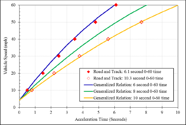
FIGURE F.4 Generalized wide-open-throttle acceleration curve.
generalized relation: one curve for a relatively slowly accelerating vehicle (10.3 second 0-60 mph time) and one curve for a relatively quickly accelerating vehicle (6.1 second 0-60 mph time).40 These two curves span the range of 0-60 mph acceleration times associated with the six vehicle platforms evaluated in this project. The specific acceleration data for the two curves were generalized by expressing the time associated with each time/velocity data point as the fraction of total 0-60 mph time. For example, a data point indicating the vehicle velocity at a time of two seconds would be expressed as 2/6.1 (or 0.328) for the 6.1 second 0-60 mph curve, signifying the velocity at 32.8 percent of the total acceleration time. This effectively creates a dataset that is independent of any given 0-60 mph time, and can thus be used to investigate whether a reliable generalized curve can be developed. The resulting data were aggregated and subjected to regression analysis to derive the generalized relation presented above (and graphically depicted for three specific 0-60 mph times in Figure F.4). As indicated there, the fit is quite good (the actual r2 for the analysis is 0.997), implying that any error resulting from the use of a generalized acceleration curve is small relative to actual vehicle-specific acceleration decay functions.41
Using the generalized acceleration decay curve function, tractive energy requirements can be estimated over the performance cycle in exactly the same manner as described above above for the CAFE cycles. Estimated tractive energy required during each second of the performance cycle is equivalent to the power required during that second.42 The maximum power estimated over the performance cycle is an indicator of the peak power required at the wheels. Peak power at the wheels is then converted into peak required engine (or alternative energy source) power in exactly the same manner as described above for the “second step” of the CAFE fuel economy modeling process employed for this project. This allows for a reasonable estimation of the engine (or alternative power source) peak output required to achieve the same level of vehicle performance as observed for baseline ICE vehicles.
Table F.24 presents a summary of the baseline performance data and associated performance cycle estimates for the six baseline vehicle platforms evaluated in this project. As indicated, the performance cycle power estimates are generally within ±6 percent of rated power, with the exception of the Chrysler 300, which differs by 10 percent. Since neither the reported 0-60 mph times nor the performance cycle power estimates are precise, the specific source of “error” is unknown. However, given the relative imprecision of the estimation approach employed, the level of estimation accuracy is
_____________________________
41 Note that the “fit” depicted in Figure F.4 is actually not precise, since the 6.1 second regression data are plotted relative to a 6 second generalized curve, and the 10.3 second regression data are plotted relative to a 10 second generalized curve. Nevertheless, the fit of the data to the generalized curves is sufficiently evident that the only marginally different generalized 6.1 and 10.3 second curves are omitted for clarity.
42 For example, power (P) in watts is equal to energy (E) in newton-meters per unit time in seconds. If we evaluate energy requirements at a frequency of 1 hertz (i.e., once per second), then P = (E / seconds) × 1 second = E.
TABLE F.24 Vehicle Performance Data
| Performance Parameter | Toyota Yaris | Toyota Camry | Chrysler 300 | Saturn Vue | Grand Caravan | Ford F-150 | |||
| 0-60 mph Time (seconds) | 10.7 | 8.8 | 6.9 | 10.4 | 9.3 | 7.7 | |||
| Engine Rated Power (hp) | 106 | 158 | 250 | 169 | 205 | 300 | |||
| Performance Cycle Peak Power (hp) | 101.7 | 163.5 | 224.9 | 159.2 | 193.2 | 314.2 | |||
| Performance Cycle Power Deviation | –4.1% | +3.4% | –10.0% | –5.8% | –5.8% | +4.7% | |||
quite good. In all cases, the predicted performance cycle power is calibrated to match the rated power of each vehicle platform engine, and all alternative scenario and vehicle architecture estimates are evaluated on a relative basis only, so that all unbiased estimation error will “cancel out” in across-scenario comparisons.
F.3 BATTERY VEHICLES
Electric vehicles have been around since the 19th century and originally were more popular than gasoline vehicles. Electric vehicles were much easier to start and did not require shifting gears, which was difficult with the transmissions of the time. However, EVs were slow, had very limited range, and required electrical power to recharge, restricting their use mainly to cities. Sales peaked in 1912 as the technology of gasoline vehicles and fuel improved.43 In recent years, interest in EVs has greatly increased, because they can operate in part or wholly without petroleum-based fuels, and because they emit no pollutants at the point of use.
Electric vehicle battery packs consist of two main components: the battery cells and the battery management system (BMS) that controls the operations of the cells and interfaces with the vehicle electronics. Cells are likely to cost about two-thirds of the cost of the pack, while the BMS plus structural components and assembly will account for the remainder. Battery cells are discussed first and the BMS later in this section.
F.3.1 Hybrid and Electric Vehicles
Two types of vehicles use externally charged batteries for propulsion: PHEVs and BEVs. Each has a rechargeable battery designed for a specific service.
PHEVs such as the Chevrolet Volt (also called an extended-range electric vehicle) have an electric motor powered by a lithium-ion (Li-ion) battery coupled to a gasoline-powered generator. They also have a conventional lead acid battery to start the gasoline engine and power accessories. When the Li-ion battery is depleted, the gasoline engine starts and charges the battery, which continues to power the car to give a greatly extended range. The engine is not used to power the car directly. The Volt has a range of about 35-40 miles on battery power alone and 375 miles total before refueling. The Li-ion battery has storage capacity of 16 kWh, which can be recharged by plugging the car into an electrical outlet. With a conventional household 120 volt (V) outlet, the battery can be fully recharged in about 10 hours. A 240 V outlet can charge it in about 4 hours. The battery is warranted for 8 years and 100,000 miles, but its capacity is expected to deteriorate by about 20 percent over the warranty period. The Volt currently costs about $39,000, about $16,000 more than a well-equipped Chevrolet Cruze, a similar
_____________________________
43 See http://en.wikipedia.org/wiki/History_of_the_electric_vehicle. Accessed March 2012.
conventional car.44 The cost to manufacture the battery cells, the price to General Motors, and the cost of assembling the battery pack are all proprietary, but the total cost is reported to be about $8,000 ($500/kWh).45 This cost is consistent with battery prices for the Tesla model S BEV, introduced in 2012. That model offers three battery options: 40 kWh for the base, 60 kWh for an additional $10,000 ($500/kWh for the upgrade), and 85 kWh for another $10,000 ($400/kWh).46
An alternative configuration, such as the Toyota Prius plug-in, has the same parallel electrical/mechanical drive configuration as the current Prius HEV but a much larger battery (although smaller than the Volt-type PHEV). The Prius PHEV should be able to drive 10-15 miles on the battery alone. The engine can drive the wheels as well as charge the battery.
The Nissan Leaf is an example of all-electric propulsion. It is powered by a 24 kWh Li-ion battery and has a range of about 100 miles. The Leaf can be charged from a household 120 V outlet, but a 240 V charging port is recommended to reduce the time required. The Leaf is connected to the port with a special outlet and plug developed by the Society of Automotive Engineers and agreed to by all manufacturers. The Leaf battery pack costs about $12,000 ($500/kWh).47
Other manufacturers are planning to introduce EVs of both types over the next several years. Improvements in battery technology will be critical to the success of EVs.
F.3.2 Batteries for Plug-In Hybrid and Electric Vehicles
Lead acid batteries have been the dominant technology for starting engines and powering accessories for a century. As the only available technology, they were used in attempts to revive EVs in the 1990s, but they proved inadequate. Nickel-metal hydride (Ni-MH) batteries with better energy storage capabilities were developed and used successfully in the first generations of HEVs. They have excellent high rate capability and long cycle life, are very robust, and can withstand abuse conditions without damage. However, Ni-MH batteries are also too heavy and bulky for the greater energy demands of PHEVs and BEVs.
Table F.25 summarizes the energy storage capability of the principal vehicle battery systems. While the Li-ion battery has higher energy density, it costs more than the lead acid batteries, because it uses more expensive materials. Unlike lead acid, the term Li-ion does not define a unique system. New materials, such as silicon-Li alloy anode and layered Ni-Co-Mn oxide cathode materials with higher energy density are under development, as are new cathode materials, although they may cost more and are unproven in vehicle operation.
There is general agreement that the Li-ion battery will be the battery of choice for EVs. It was developed specifically for the portable electronics industry 20 years ago because of its light weight, superior energy storage capability, and long cycle life—attributes that also are important for EVs. Cell performance has increased steadily with improvements in the internal electrode structure and cell design and manufacturing processes, as well as the introduction of higher-performance anode and cathode materials. Evolution of the technology is shown in Figure F.5.
_____________________________
44 See http://www.chevrolet.com/volt-electric-car/. Accessed February 2012.
45 H. Takeshita, Tutorials at the 28th and 16th International Power Sources Seminars, The International Battery Seminar, LLC, Boca Raton, Fla., March 2011.
46 See http://www.teslamotors.com/models/options. Accessed March 2012. Note that costs are not the same as prices, which may include markups and/or subsidies.
47 Press release, Nissan press Release 2011 DOE Annual Merit Review May 9-13, 2011, presentation.
TABLE F.25 Typical Cell Characteristics in 2010
| System | Wh/l | Wh/g | $/h | Comments | |||||
| Lead acid | 80 | 25 | 0.05 | Reliable, low cost | |||||
| Battery for the EV1 | |||||||||
| Ni-MH | 430 | 90-100 | 0.35 | Hybrid battery of choice | |||||
| Replacement by Li-ion likely | |||||||||
| Li-ion | 570 | 203 | 0.20 | Graphite anode, lithium cobalt oxide cathode, | |||||
| LiPF6 organic solvent electrolyte | |||||||||
SOURCE: T.B. Reddy, ed., Lindens Handbook of Batteries, McGraw Hill, 2011.
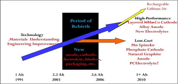
FIGURE F.5 Improved performance of lithium-ion 18650 cells.
The 18650 cell is typical example of the Li-ion technology. It is a cylinder 18 mm in diameter and 65 mm high, somewhat smaller than the size of a standard D battery. Originally, a lithium cobalt oxide cathode and a hard carbon lithium intercalation anode produced 3.6 V open circuit voltage. In 1991, the cost of the 18650 was $3.17/Wh. Twenty years later in 2010, the same cell cost $0.20/Wh, while the capacity of the cell had increased from 1 Amp-hour (Ah) to over 3 Ah in the same volume. These improvements resulted from the introduction of new, high-performance materials, improvements to the cell and electrode structure design, and high-volume production processes with reduced wastage. As a rule of thumb for highly automated cell production, cell materials constitute about 80 percent of the cost of the cell.48 During the period 1991-2010, production increased from about 30 million to over 9 billion cells annually. After 20 years, designs, manufacturing processes, and economies of scale had matured, and costs have leveled out. In the time period 2004-2005, new anode and cathode materials were introduced to continue the growth in energy storage capability. The DOE battery research and
_____________________________
48 As used here, “materials” means processed materials ready for cell manufacture. It does not mean raw materials, which may be much cheaper. The processing of these materials is subject to considerable cost reduction, as is the cell manufacture.
development (R&D) programs are expected to result in a steadily increasing performance and materials. In the outer years, new battery chemistries, such as lithium-air, would significantly increase performance and the range between the need for recharging.
This pattern of cost reduction is typical for high-volume battery cell production. Cells for vehicles are likely to be prismatic (flat plate) or pouch-type rather than cylindrical, because these are easier to cool and arrange in stacks. The production process for flat plate cells differs from that for cylindrical cells, but it is anticipated that the cost will follow a similar learning pattern as the 18650 cell. An initial high cost is expected to be followed by cost reductions from improved production efficiency in cells and materials as the process matures.
The newer higher performance cathode, anode, electrolyte, and separator materials under development today are more expensive but should follow the same learning curve for cost reduction as for the original graphite anode and cobalt cathode, electrolyte, and separator materials as the processes are refined and electrode design parameters are understood.
Unlike lead acid batteries, which all use the same set of chemicals for the anode and cathode, many different chemistries are used to construct Li-ion cells, as shown in Table F.26. Thus, it is necessary when discussing the Li-ion system to keep in mind the composition of the anode and cathode active materials.
Each cell chemistry has its own unique characteristics of chemistry, particle size, reactivity, safe operating envelope, etc., that must be adapted to the production process. Several different chemistries may be used as HEVs, PHEVs, and BEVs emphasize different characteristics in their batteries. The choice of the active materials and cell design determine its energy storage capability. The total available energy in a battery is governed by thermodynamics of the electrode reactions. Thinner, high surface area electrodes are preferred for efficient usage of the active materials, but result in lower energy storage (Wh/cc and Wh/kg). Thicker electrodes offer higher Wh/kg and Wh/cc, but result in a lower efficiency of material usage at the high current demands of PHEV and BEVs. The life of the battery is limited by the volume expansion-contraction of the anode and cathode materials during charge and discharge, leading to loss of contact with the current collector in the electrode structure. The battery pack assembly of the individual cells requires sophisticated control circuitry to protect the pack from rogue cells that could disrupt normal operation. Battery pack design and assembly is discussed below.
In selecting cells for the battery pack, a trade-off is often made between higher voltage and higher capacity cell technology (such as nickel cobalt aluminum or layered manganese nickel cathode) versus lower capacity but lower cost (such as the lithium manganese spinel or lithium iron phosphate based technology with longer cycle life). Both the Volt and Leaf employ the manganese spinel cathode and graphite anode in a flat-plate configuration with LiPF6 electrolyte for long cycle life and relatively low cost.
F.3.3 Automotive Battery Packs
The battery pack for vehicles consists of two main components (1) an assembly of cells to meet the design requirements for total energy (kWh) and voltage and (2) a BMS to control its operation. A typical pack might consist of several hundred cells configured in series strings to achieve the design voltage, with sufficient strings in parallel to achieve the design energy. Cells represent 50-70 percent of the cost of battery packs. The BMS plus structural components and assembly are responsible for the rest.
The safe operating parameters for each type of cell must be established, and the BMS must be designed to maintain the cells within those parameters for long life and safe operation of the battery. The goal of 10 to 15 years service for automotive applications is far longer than for use in electronic devices and approaches that required for avionic applications. The BMS senses the temperature, current flow, and voltage of each individual cell in the pack. Depending on the particular company’s design, the BMS can isolate an individual cell that deviates from prescribed limits to prevent damage to the battery. It also controls the cooling system required to prevent overheating of the cells during charging or discharging.
TABLE F.26 Characteristics of Lithium-Ion Batteries Involving Different Chemistries
| Characteristics | Cathode/Anode | ||||||||
| Nickel Cobalt Aluminum Oxide/ Graphite | Manganese Spinel/Graphite | Iron Phosphate/ Graphite | Manganese Spinel/Lithium Titanium Oxide | ||||||
| Durability | Good | Fair | Good | TBD | |||||
| Power | Fair | Fair | Good | Good | |||||
| Energy | Good | Good | Fair | Poor | |||||
| Safety and abuse tolerance | Poor; safety concerns | Fair | Good | Good | |||||
| Cell voltage | 3.6 | 3.8 | 3.3 | 2.5 | |||||
| Some battery developers | Johnson Controls/Saft | LG Chem Ltd. | A123 | EnerDel | |||||
| Associated vehicle manufacturers | Toyota/Ford | GM | Daimler HEV buses | ||||||
NOTE: Cathode chemistries are frequently referred to as involving a spinel crystal structure. Actually there are no pure spinel structures present in Li-ion batteries; spinel-like would be more accurate.
SOURCE: Transitions to Alternative Transportation Technologies; Plug-in Hybrid Electric Vehicles. The National Academies Press, Washington, D.C. 2010. Available at http://www.nap.edu/catalog.php?record_id=12826.
Cooling can be by air or liquid. The latter is more expensive but maintains better thermal control, which may be important for longer cell life. Adequate cooling is particular important if the battery is being charged rapidly in hot weather because a significant amount of heat is generated within the pack.
It is commonly understood that a cell internal fault (e.g., short) is a “single-point-fault” type such as occurs in a cell separator failure, allowing the anode to contact directly the cathode creating an internal short in a single cell. Since all cells in the pack are a part of the circuit, the entire energy stored in the battery pack can be released in that single shorted cell, with the potential for critical results. It has long been accepted that you cannot just reduce the likelihood of a single-point-fault to the level necessary to provide the needed safety; nor can one verify that a single-point-fault “just will not happen.” However, with the energy-density demands of the automotive market and the use of large-format cells, it is not realistic to expect to optimize energy-density without having the possibility of a cell internal fault propagating.
The BMS enhances cell/battery safety by sensing the on-set of failure, then taking swift action for mitigation. The BMS monitors the battery and individual cells for anomalous behavior in real-time including cell voltage, cell external temperature, battery temperature, battery current, and cell balancing history. This includes rapid fault detection of cell shorting; e.g., a cell voltage “spike” and actions to isolate the fault. The BMS operates at speeds capable of accurately capturing the highest frequency effects. In effect there are three major components that characterize the safety of a battery pack: the failure rate of an individual cell, the probability of propagation of a single cell fault to the pack, and the failure rate of the electronics.
The intent is to identify impending problems and take action to mitigate accordingly, i.e., predictive mitigation. The BMS reaction time is less than 2.5 milliseconds. The BMS restricts operation of the battery to within the “operational envelope.”
In order to deduce the internal cell concentration and temperature profiles, an understanding of the cell (cell model) and an understanding of the cell operational history is required; e.g., recent charging/discharging profiles. It has also been observed that existing safety mechanisms for cells used in
consumer electronics, such as the positive temperature coefficient devices can be of little value in large format cells. More importantly, it has been observed that current interrupt devices (CIDs) for the 18650 cell can be too slow to mitigate a problem in large-format cells where the temperature increase can fully develop in some areas of the cell before the CID can react.
The propagation of an internal short induced within a single cell depends on the history of the cells in the pack as well as the immediate operating conditions. Battery temperature, cell internal temperature profile, and cell state-of-charge play a key role in holding the battery/cells within a desired “operational envelope” such that it is quantifiably less probable that a cell internal short leads to propagation. The best solution builds on understanding the bounding criteria associated with whether an internal short will or will not propagate.
Safety analysis can have both qualitative and quantitative components. Both aspects are meaningful in understanding assurance of system safety. In military and commercial aerospace, both components are fundamental to the safety analysis process. The BMS consists of programmable sensors, intelligence, communications, self-diagnosis, status reporting, and control mechanisms. Each battery block is designed to protect itself. Single-point faults are fundamentally disallowed in commercial aerospace critical systems. This is a typical requirement for any scenario where safety criticality is an issue, such as in aviation. The single-point-fault issue has a long history, including tragic events that have often been traced back to such a root cause. Exceptions to this exclusion rule are exceedingly rare.
F.3.4 Battery Technology for Future Applications
Strong research programs in national laboratories, universities, and private industry are developing new materials, lowering costs, and improving the energy storage capability of the battery. All of the components—anode, cathode, separator and electrolyte—are included in these studies. For instance, the experimental programs to develop silicon to replace graphite in the anode may significantly improve capacity. The new layered nickel-manganese-cobalt oxide materials, now under development, offer similar improvements in cathode performance but will require sophisticated production processes. These materials will be more expensive at the start but can be expected to show significant cost reduction as demand increases. In volume production, cathode materials using nickel and cobalt may have resource limitations that could result in price increases eventually.
F.3.4.1 Forecast for Cost of Electric Vehicle Batteries 2012 to 2030
Future costs of Li-ion cells for vehicles are likely to follow the trajectory of cells for electronic applications. Those costs fell in a regular manner for 10 years and then began to level off as production processes matured and improved in reliability. This is typical for a learning curve in manufacturing of batteries as the cell internal designs and production process becomes stabilized. Materials suppliers should have a similar learning curve as increased demand for materials for cell construction lead to improvements in their production. As the best battery chemistries for vehicle applications are established, and cell design and production capability is established within the United States, costs will come down rapidly at first and then more slowly. Costs of the battery pack (in addition to the cells) also should decline at about the same rate as cells as manufacturers and suppliers improve designs and production techniques.
In 2010, the United States had essentially no Li-ion cell manufacturing capability or infrastructure to support it. All cells for battery packs have been imported from Japan, Korea, or China. U.S. volume production of automotive batteries is just beginning. By 2030, cells and battery packs could become an important industry here if the manufacturing capability and supporting infrastructure are established over the next decade or two. Infrastructure in parts, materials, and trained engineers to support the industry will
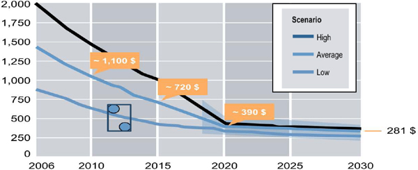
FIGURE F.6 Estimated cost ($/kWh) of lithium-ion automotive propulsion batteries for the period 2010 to 2030.
be required. A battery recycling effort will be needed when large numbers of battery packs reach the end of their useful lifetimes. Recycling works well for lead acid batteries, almost all of which are returned, and the components are used in construction of new batteries.
The projected costs in Figure F.6 start with the 2012 pack costs assumed for the Chevrolet Volt and Nissan Leaf at $0.50/Wh (or $500/kWh). The assumption is made that the cost of cells manufactured in the United States for vehicle application will decline, but not as rapidly as the Li-ion cells for electronic applications did in their early years. The cost of those cells declined more than 95 percent in 20 years. In addition, the costs of assembling the cells into packs will decline, but perhaps not as rapidly as the cells. Midrange BEV pack costs are estimated at $250/kWh (45 percent reduction from $450 in 2010). Optimistically, pack costs might reach $200/kWh (55 percent reduction). PHEV pack costs are likely to be $60/kWh to $70/kWh higher.
The production process for flat cell production is simpler than for cylindrical cell production yet requires greater precision. As production of vehicle batteries gets underway, the production process will be improved going down the learning curve for the production process for vehicle cells, as was the case for cells for electronic applications.
In 2010, mature cylindrical cell production had a defect rate of 1 in 5 million cells, based on incidents of battery failure. All of these incidents have been traced to a manufacturing defect, not a chemistry issue. As a result, safety can be expected to improve as the production process for vehicle batteries matures.
DOE has funded an intense effort to develop new higher-performance materials that lead to increased driving range on a single charge. Although cells made using the new materials give higher energy storage capability, they also increase the cost if nickel and cobalt are major components of the materials. It is expected that, with time, the cells made with new materials will undergo the same decrease in cost related to volume production. While the new materials are initially more expensive, they should follow the same learning curve with appropriate lowering in cost.
A car built as a BEV today that gets 30 mpg would require about 26 kWh/100 miles, or 260 Wh/mile. For a range of 300 miles, the battery would have to be at least 78 kWh. While not impossible (see the mention of the Tesla above), this would be prohibitively expensive, heavy, and bulky for most applications and would take prohibitively long to charge. It is difficult to envision how a Li-ion battery that large could be developed that would be feasible for general use. More advanced technologies, such as lithium-air with about 5210 Wh/kg, could be developed for automotive applications in this period, but,
even if successful, they probably will not be widely available until after 2030. If new battery technologies are not commercialized, the only alternative to achieve such a range would be to design smaller, lighter cars. If the energy demand can be reduced to about 17 kWh/100 miles, as per the efficiency measures discussed above, and if battery pack costs are reduced to $200/kWh, then longer distance travel would become more practical, in particular if batteries can be developed to withstand repeated fast charges. Otherwise, BEVs will be limited mainly to short distance travel in urban and suburban areas.
PHEV batteries are smaller than those for BEVs, so the pack cost per kilowatt-hour is somewhat higher. The optimistic estimate for 2030 is $260/kWh and the midrange is $300/kWh.
F.3.4.2 Estimation of Battery Costs in 2030 to 2050
Li-ion batteries will continue to improve after 2030 but probably at a reduced rate. Strong R&D programs are developing new cathode and anode materials, electrolytes, and separator materials, which are expected to reach maturity and yield dividends in this time period. New active materials with higher energy content, such as silicon alloy anodes and layered nickel-manganese-cobalt materials, should become available in volume production. Materials account for about 80 percent of the cost of Li-ion cells in high-volume production. Hence, cost reduction will largely focus on materials used to produce the cells. In addition, the DOE program to support the electric vehicle application can be expected to deliver higher-performance materials that potentially will lower costs. The practical cost limit of Li-ion cells is probably about $80/kWh, and the corresponding pack cost would be $150-$160/kWh.49
As R&D improvements continue with government support, new high-energy materials and new electrolytes are being developed. This may led to next-generation technologies such as high-energy lithium-sulfur and lithium-air systems using a fuel cell oxygen cathode and lithium metal anode. Another long-term option is the flow cell, such as the semi-solid lithium rechargeable flow battery.50 At this writing, these systems are still in an advanced research stage but not commercialized.
The lithium-air, in particular, has received significant attention. Lithium metal has the highest voltage and capacity of any anode material, and oxygen in aqueous electrolyte is an excellent low-cost catalyst with good performance. A significant effort is underway to develop the system into a commercial product. Most approaches use a ceramic barrier between the two electrodes to prevent water from reaching the lithium metal anode. Although the challenge is difficult, significant progress has been made. However, the committee does not believe that the chances of commercial success of any of these advanced batteries are high enough to warrant inclusion in its scenarios.
While the exact route to low-cost cells and batteries is not clear, it should be possible to reach a cost of $160/kWh in 2050 for automotive propulsion cells. Figure F.7 shows a possible cost trajectory. An optimistic projection is $150/kWh. Only with volume manufacturing of the battery cells, electrolyte separator, and cathode materials will these cost targets be met. PHEV batteries are estimated to be about $40/kWh higher.
All of the cell materials can be used for multiple applications. If the goal of $150/kWh can be met for automotive use, then electronic cells should have the same cost structure. In addition, they should benefit from increased reliability. Defect-free, uniform cell-to-cell output with 10-8 reliability will be required for automotive batteries to meet reliability and safety requirements—significantly higher than what is required for electronic cells.
_____________________________
49 ARPA-E’s BEEST Program: Ultra-High Energy, Low Cost Energy Storage for Ubiquitous Electric Vehicles, presentation to the committee by David Danielson, Program Director, ARPA-E, March 21, 2011.
50 Dudata, M., et al., Semi-Solid Lithium Rechargeable Flow Battery, Advanced Energy Materials, Vol. 1, Issue 4, July 2011.
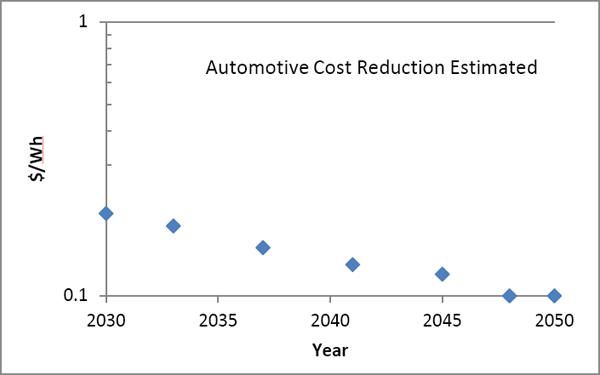
FIGURE F.7 Cost for automotive batteries in the time period 2030 to 2050.
F.3.5 Barriers to the Widespread Adoption of Electric Vehicles
The main problems facing the use of EVs are:
1. The high cost of the battery,
2. The lower driving range relating to the fundamental lower energy storage capability of the battery compared to gasoline,
3. Improving the durability and longevity of the batteries,
4. Ensuring safety, and
5. Establishing a domestic vehicle battery industry.
Solving all these issues simultaneously will be difficult.
F.3.5.1 Battery Cost
Battery cost is a key issue for the success of the electric vehicle. Lower cost electrode materials will be an important step. Cathode, separator, and electrolyte are the main contributors to the cell cost. Most of the new cathode materials are composed of high-cost nickel and cobalt materials. However, there are lower cost, lower performance materials such as lithium iron phosphate and manganese spinel cathode coupled with graphite anode materials that can be made for about $10/kg or less in large volume. Even with low-cost materials, there is a learning curve for manufacturing that progressively lowers cost, based on identifying slow and costly processes and improving on them.
Economy in manufacturing requires automated production capability to achieve repeatability and uniform capacity cell-to-cell, essential for safe operation in automotive applications and a long life requirement. The new cell designs are prismatic, not cylindrical as for the electronic applications, and have a different production process than the cylindrical electronic cells. The process is somewhat simpler but requires greater emphasis on process control and lower cost materials.
There has been no U.S. production of Li-ion automotive cells until recently with the opening of the A123 facility in Michigan. Li-ion cells are produced in Asia, where a trained workforce exists, and imported for assembly into packs in the United States. There is no infrastructure for materials components
or a skilled workforce base in the United States, and these must be re-established for the U.S. industry to become viable. This is a significant barrier to overcome. It takes at least 5 years for a production line to become fully operational. It takes a similar period to train a workforce. Overall, it will take 5 to 8 years and significant capital investment to re-establish this infrastructure, but it is essential for a viable Li-ion battery industry capable of competing in the world market.
F.3.5.2 Battery Performance
Battery performance must be improved if BEVs are to widely replace ICE vehicles. The present average auto has a range of about 300 miles on a tank of gasoline. Very few affordable BEVs will greatly exceed 100 miles for the next several years. That will be adequate for some drivers for some applications, but many people will not be willing to accept that limitation. Lighter, more efficient vehicles will be developed, extending the range or lowering the size and cost of the battery for the same range, but it will also be important to squeeze more performance out of batteries without compromising cost. If the range most EVs can travel without lengthy recharging is no more than 100 miles, they will be limited largely to local travel in an urban or suburban environment.
F.3.5.3 Durability and Longevity
Durability and longevity are functions of both design and manufacturing precision. Exchange current is the fundamental rate at which electrode reactions function in a reversible manner. Higher currents stress the reaction on both charge and discharge and often cause formation of unwanted and possibly damaging changes in the reaction mechanism. For instance, forcing the graphite negative to recharge quickly can result in lithium depositing on the surface rather than entering into the lattice. This lithium metal reacts directly with the electrolyte, depositing unwanted reaction byproducts that block the surface and increasing the current density at other parts of the electrode, permanently damaging cell operation. Thus, rapid charging and discharging can shorten the lifetime of the cell.
Poorly designed porous electrode structures can lead to lower performance. The mixture of conductive diluent, binder, and active material should result in a uniform reaction throughout the electrode structure. Any blockage in the porosity reduces the ability to deliver high-current pulses and lowers the capacity of the electrode.
Volume changes during charge and discharge introduce stress inside, with movement of electrodes in cylindrical cells. Cell design for long life must accommodate the volume change in present cell materials. Low-cost phosphate and spinel materials have a minimum volume change but have low energy content. The volume change introduces stress inside the cell and can limit cycle life.
F.3.5.4 Safety
Safety of the battery is a critical issue. The recent Volt fires, although not a result of operational failures, are a reminder that the safety questions must be addressed. There is no long-term experience with commercial automotive batteries. For the 18650 size Li-ion cell used in electronic applications, the failure rate is about 1 in 5 million cells, some of which led to laptop computer fires. All incidents have been traced to manufacturing defects. This rate is not acceptable for automotive applications, and significant efforts must be made to improve the production processes to produce a higher quality cell in keeping with established failure rate of 10-8.
Li-ion cells are highly energetic and contain sufficient energy to heat the cell to more than 500°C if released rapidly inside the cell. That could cause neighboring cells to also fail, leading to a catastrophic event. The failure rate for Li-ion 18650 cells equates to a reliability rate of about 99.9999 percent. This
level of reliability is not satisfactory for electric vehicle batteries where 99.999999 percent is the minimum required.51 Therefore, it is essential that cell construction defects in the individual cells, as well as defects in the battery pack itself, are eliminated so that a catastrophic event “will not happen.” Testing is required to prove that the battery will meet the standard.
One additional potential barrier may also deter drivers from buying BEVs is future reliability of the electrical grid. As discussed in Chapter 3, the grid has been very reliable and will be capable of charging many millions of EVs if charging is done at night. However, outages of days and weeks are possible. Under such conditions, BEVs could be unavailable (PHEVs could still operate). Fast charging by many people at the same time, i.e., on returning from work, will place an additional strain on the grid system as well, possibly leading to increased vulnerability of the grid.
F.3.6 Electric Motors
Essentially all HEVs, PHEVs, and EVs use rare-earth-based interior permanent magnet (IPM) motors. These rare earth magnets were invented and produced initially at General Motors Research Laboratories, which developed and patented a high-flux magnet material using rare earth materials termed “MagnaQuench” for neodymium-iron-boron (NdFeB). These magnets have almost an order of magnitude greater flux than other types of permanent magnets and created a revolution for many products that needed small high-flux magnets, including speakers, hard drives, etc.
There were significant price reductions after the MagnaQuench patent expired in the 1990s. The production of rare-earth magnets then moved from the United States to Japan. In 2000, China lowered rare-earth prices to levels that others could not match. Finished magnets were selling for less than $16 per kilogram. China ended up with a market share of more than 90 percent and, effectively, a monopoly on rare-earth-magnet materials. In 2008, China raised the price of rare-earth magnet materials and has steadily increased the price, reaching as high as $60/kg. An automotive traction motor uses 1 to 1.5 kg of rare-earth-magnet materials, which strongly influences the cost of motors for EVs. The rare-earth alloys are also used in the hydrogen-absorbing cathode in the Ni-MH battery used in electronics and in hybrid vehicles.
IPM motors are by far the most popular choice for hybrid and EVs because of their high power density, specific power, and constant power-speed ratio (CPSR). Performance of these motors is optimized when the strongest possible magnets (e.g., NdFeB) are used. Cost and power density (power density criterion translates to torque density and acceleration) are emerging as the two most important properties of motors for traction drives in hybrid and EVs, although high efficiency and specific power are essential as well.
China has the largest rare-earth resources in the world and currently controls the supply of rare-earth-materials mining and processing. Whereas China previously supplied rare-earth metals to other countries for magnet production, it recently vertically integrated to include magnet and motor production, instead of exporting the rare earth ore. China also announced its intention to limit exports on rare-earth materials in order to ensure a supply for their own needs, and it has used its control of rare earths as a foreign policy tool. There is always the distinct possibility that a limited supply and/or very high cost of rare-earth magnets could make these materials unavailable and/or too expensive outside China.
Rare-earth mines in the United States were shut down in about 2000. The United States produced rare earth materials mainly from the Molycorp Mountain Pass mine in California. Recently, MolyCorp announced that the Mountain Pass mine, which has a significant reserve of rare earth ores, is being reactivated. However, restarting mining operations will require a significant capital investment and time. Once in operation, the Mountain Pass mine could supply the rare earth needs of North America for a decade or more. Molycorp also announced finding significant new deposits near its mine in California.
_____________________________
51 H. Takeshita, Tutorials at the 28th and 16th International Power Sources Seminars, The International Battery Seminar, LLC, Boca Raton, Fla.
The potential shortage of rare earths has driven DOE to examine the role of permanent magnets in electric machines and technologies that could either eliminate or reduce the need for rare-earth magnets. The DOE strategy involves three parallel paths:
1. If there is a reasonable chance that rare earth magnets will continue to be available, either from sources outside China or from increased production in China, then development of IPM motors using rare earth magnets should be continued with emphasis on meeting the cost target.
2. Since there is a possibility that rare earth magnets may become unavailable or too expensive, the effort to develop new designs for permanent magnet motors that do not use rare earth magnets needs to be continued. Other possible magnet materials include samarium-cobalt, Alnico, and ferrites. Alternatively, efforts to develop motors that do not use permanent magnets but offer attributes similar to IPM motors are encouraged.
3. New magnet materials using new alloys or processing techniques that would be less expensive or have comparable or superior properties to existing materials should be developed if possible.
Recently Toyota announced that it has developed a new material that has equivalent or superior capability in as a substitute for the rare earth materials in electric motors for its line of EVs (Reuters, 2012) (5). Toyota could bring the technology to market in 2 years if the price of rare earths does not come down. Toyota has developed an induction motor that is lighter and more efficient than the magnet type motor now used in the Prius and does not use rare earth materials. The present Prius has more than 20 pounds of rare earth materials.
For the past several years, the IPM motor has been considered the obvious choice for electric traction drive systems. However, with the rapidly increasing costs of magnets and the possibility of a future shortage of rare-earth metals, the use of IPM motors would not be economical or technically feasible.
Surface-mounted permanent magnet motors have relatively high specific power but restricted CPSR. The speed of these motors is limited due to challenges of magnet retention. Essentially, they have no advantage over IPM motors. Induction motors have lower power density compared with IPM motors but also cost less. They are robust and have a medium CPSR. Being a mature technology, they are reliable but have little opportunity for improvement. Most manufacturers consider induction motors the first choice if IPM motors are not available.
Switched reluctance (SR) motors are durable and low cost, and they contain no magnets. Their efficiency is slightly lower than that of IPM motors at the “sweet spot,” but the flatter profile of SR motors can give higher efficiency over a typical drive cycle. The torque density of SR motors is much better than that of induction motors. They require different power electronics compared to IPM motors. Significant concerns about SR motors are torque ripple and acoustic noise. Efforts are currently being directed to solve those problems through rotor design, modified electronics, and stiffening of the housing.
For the past several years, the IPM motor has been considered the obvious choice for electric traction drive systems. However, with the rapidly increasing costs of magnets and the possibility of a future shortage of rare-earth metals, the use of IPM motors may not continue to be economically or technically feasible. Table F.27 estimates the future costs of electric motors, assuming such shortages do not occur.
TABLE F.27 Projected Fixed and Variable Cost Coefficients for the Motor System
| HEV/PHEV | BEV/FCEV | ||||||||
| Fixed | Variable/kW | Fixed | Variable/kW | ||||||
| Midrange case–US $ | |||||||||
| 2010 baseline | $668 | $11.58 | $668 | $11.58 | |||||
| 2015 average of 2010 and 2020 | $586 | $10.38 | $586 | $10.38 | |||||
| 2020 $4%/2% electronic/other | $504 | $9.18 | $504 | $9.18 | |||||
| 2025 average of 2020 and 2030 | $449 | $7.74 | $464 | $8.24 | |||||
| 2030 1% learning+motor integration | $393 | $6.30 | $425 | $7.30 | |||||
| 2035 1% learning | $374 | $5.99 | $404 | $6.95 | |||||
| 2040 1% learning | $356 | $5.70 | $384 | $6.60 | |||||
| 2045 1% learning | $338 | $5.42 | $365 | $6.28 | |||||
| 2050 1% learning | $322 | $5.15 | $347 | $5.97 | |||||
| Optimistic case–US $ | |||||||||
| 2010 baseline | $668 | $11.58 | $668 | $11.58 | |||||
| 2015 average of 2010 and 2020 | $586 | $10.38 | $586 | $10.38 | |||||
| 2020 $4%/2% electronic/other | $504 | $9.18 | $504 | $9.18 | |||||
| 2025 average of 2020 and 2030 | $427 | $7.34 | $442 | $7.84 | |||||
| 2030 1% learning+motor integration | $349 | $5.50 | $381 | $6.50 | |||||
| 2035 1% learning | $332 | $5.23 | $362 | $6.18 | |||||
| 2040 1% learning | $316 | $4.97 | $344 | $5.88 | |||||
| 2045 1% learning | $301 | $4.73 | $327 | $5.59 | |||||
| 2050 1% learning | $286 | $4.50 | $311 | $5.32 | |||||
F.3.7 Cost and Performance Evolution of a Battery Electric Vehicle
A complete shift to battery propulsion eliminates the ICE drivetrain and its inefficiencies (and costs), although the new electrical components—and especially the battery—are expensive and are not without inefficiencies. However, the committee foresees that all components of the BEV drivetrain—and especially the battery—will improve in performance (e.g., achieve higher energy and power density) and achieve significant cost reductions over the 2010-2050 period. Battery costs are the key factor in electric vehicle cost effectiveness. Although projections of future battery costs are quite uncertain, the committee believes these costs, approximately $500/kWh in 2010, can be reduced to $200-$250/kWh by 2030 and $150-$160/kWh by 2050 (Table F.28). In addition, the combination of increasing efficiency of the electric drivetrain, the substantial decreases in vehicle loads, and the expected increase in the allowable battery depth of discharge (about 80 percent in 2010, 90-94 percent by 2050) reduce the amount of battery capacity needed to achieve a fixed range. For example, the battery capacity needed to attain about 100 miles in on-road capacity for a Camry-sized car is about 38 kWh in 2010 but shrinks to 16 kWh (optimistic) to 20 kWh (mid-level) by 2050 in the two scenarios examined. If EV performance and cost follow the path shown in Table F.28, the cost penalty of a 100-mile range EV compared to a conventional drivetrain vehicle will shrink from its current level of about $16,000 to $2,000-$3,000 by 2030, and the EV will become the less expensive than its conventional counterpart by 2050. In addition, the gasoline-equivalent fuel economy of such a vehicle—already high at about 150 mpg (EPA test) in 2010—can rise to 195-225 mpg by 2030 and 250-300 mpg by 2050.
TABLE F.28 Details of the Potential Evolution of a Midsize Battery Electric Vehicle, 2010-2050
| 2010 | 2030 mid | 2030 opt | 2050 mid | 2050 opt | |||||
| Test cycle range, miles | 130 | 130 | 130 | 130 | 130 | ||||
| Electric motor power, kW | 110.8 | 91.6 | 85.6 | 81 | 71.2 | ||||
| Fraction of braking energy recovered, % | 87.5 | 90.2 | 92.5 | 94 | |||||
| Electric motor efficiency, % | 90.7 | 91.6 | 92.5 | 93.5 | |||||
| Net battery charge efficiency, % | 86.7 | 87.8 | 88 | ||||||
| Accessory demand, W into generator | 152 | 104.1 | 98.2 | 92.3 | 84.6 | ||||
| Battery depth of discharge, % | 80 | 88 | 92 | 90 | 94 | ||||
| Battery capacity, kWh | 37.6 | 25.8 | 21.7 | 19.9 | 15.9 | ||||
| Fuel economy, test mpge | 152 | 195 | 225 | 250 | 303 | ||||
| Fuel economy, test kWh/100 mile | 22.1 | 17.3 | 15 | 13.5 | 11.1 | ||||
| Battery cost, $/kWh | 450 | 250 | 200 | 160 | 150 | ||||
| Incremental cost versus baseline, $ | 15,979 | 5,401 | 4,384 | 3,184 | 2,050 | ||||
| Incremental cost versus conventional, $ | 15,979 | 2,968 | 2,139 | –475 | –1,353 | ||||
F.4 HYDROGEN FUEL CELL ELECTRIC VEHICLES
F.4.1 Hydrogen Fuel Cell Electric Vehicles in 2010
F.4.1.1 Fuel Cell Powertrain
A typical FCEV powertrain schematic is shown in Figure F.8. As in hybrid vehicles, a battery in FCEVs enables regenerative braking and supplements the fuel cell system in meeting transient on-road power demands (including start up). It thereby enables the fuel cell to be sized for nominal driving requirements and efficient operation. This battery is larger than those currently used in HEVs, because it must power driving for 2-5 miles while the fuel cell warms up in cold weather. It is recharged from the fuel cell directly and through regenerative braking. Future improvements in the performance and cost of HEV batteries will apply to FCEVs as well.
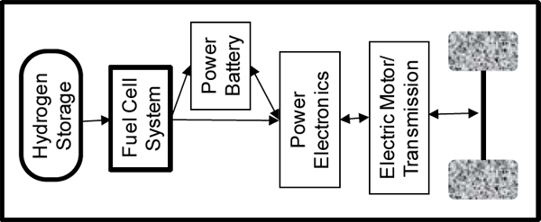
FIGURE F.8 Typical FCEV powertrain schematic.
Over the past decade, FCEVs in demonstration fleets have shown significant technology advances toward commercial readiness in the areas of performance and cost. For example (James et al., 2010; EPA, DOT, CARB, 2010; Carlson et al., 2005; Kromer and Heywood, 2007; Bandivadekar et al., 2008), the cost of automotive fuel cell systems has been reduced from $275/kW in 2002 to $51/kW in 2010 (based on projections of high-volume manufacturing costs); on-road vehicle durability has doubled since 2006 to 2,500 hours (equivalent to approximately 75,000 mile range); and vehicle range has increased to at least 300 miles. Vehicles have demonstrated the capability to meet all urban and freeway driving demands. The remaining advancement under development is high load driving at high ambient temperatures.
F.4.1.2 Fuel Cell Systems
Fuel cell stacks currently used in automotive applications are based on the polymer-electrolyte membrane/proton-exchange membrane (PEM). PEMs operate at moderate temperatures that can be achieved quickly so they are suitable for the infrequent and transient usage of on-road automotive service. Structured catalysts using precious metals as the active catalytic materials (primarily platinum) convert hydrogen gas and air into internal carriers of electric charge at the anode and cathode, respectively. A separation membrane transports hydrogen ions from the anode to the cathode. Improvements in stack durability, specific power, and cost have resulted from methods to improve the stability of the active catalytic surface area and from new membrane materials and structures. For example, stack lifetimes of 1,000-2,500 operating hours have been demonstrated in on-road vehicles, and short-stack laboratory tests with newer membrane technologies have demonstrated (using accelerated test protocols) over 7,000 hours. In addition, improvements in stack durability and efficiency have resulted from continued reduction of stack mass transport losses due to improved hydrogen and air flow management and membrane hydration management and improved efficiency and durability of electrode structures.
The balance of plant (BOP) consists primarily of mature technologies for flow management of fluids and heat. Significant improvements in efficiency and cost result from continuing simplifications in BOP design.
Further reductions in the cost of fuel cell systems are expected to result from downsizing associated with improved stack efficiency and improved response to load transients. Significant additional cost reductions will result if vehicle loads (weight, rolling resistance, and aerodynamics) are reduced, because that will allow the use of smaller hydrogen tanks and fuel cells with lower total power.
F.4.1.3 Fuel Cell System Efficiency: 2010.
Fuel cell system efficiency measured for representative FCEVs driven on chassis dynamometers at several steady-state points of operation has shown a range of first-generation net system efficiencies from 51 to 58 percent (Wipke et al., 2010a, b). Second-generation vehicle systems have shown 53 to 59 percent efficiency at one-quarter rated power, as illustrated in Figure F.9. System efficiency has improved slightly while the major design changes have focused instead on improving durability, freeze performance, and cost (Wipke et al., 2010a, b).
With current fuel cell system efficiencies, fuel storage capacity and vehicle attributes (weight, aerodynamics, and rolling resistance), FCEVs are currently capable of 200-300 miles driving range and fuel efficiency over twice that of the comparable conventional ICEV. Examples include the 20 mpg 2007 Chevrolet Equinox, which, when equipped as an FCEV, achieved 45 mi/kg-H2 (1 kg of H2 is the energy equivalent of 1 gallon of gasoline). Similarly, the 2011 Honda Clarity FCEV achieves more than 60 miles/kg-H2, but an equivalent ICEV would have gotten only 27 mpg.
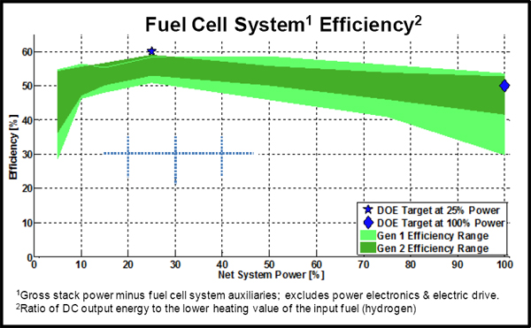
FIGURE F.9 Demonstrated efficiency of vehicle fuel cell systems.
SOURCE: Wipke et al. (2010a,b).
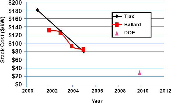
FIGURE F.10 Historical progression of high-volume fuel cell stack cost projections.
SOURCES: Tiax (Carlson et al., 2005; Ballard Power Systems, 2006).
F.4.1.4 Fuel Cell System Cost: 2010
Detailed analyses of fuel cell system designs, material costs, component costs, and manufacturing and assembly costs (Carlson et al., 2005; Kromer and Heywood, 2007) previously estimated 2005 fuel cell costs to be $67/kW. But recent technology developments aimed at cost reduction and improved detailed cost analyses (James et al., 2010; Carlson et al., 2005) have resulted in estimates for high-volume fuel system cost dropping to $51/kW in 2010. The fuel cell stack generally accounts for 50-60 percent of the system cost. Figure F.10 shows how projections of costs for high-volume stack production have declined as the technology has improved. Figure F.11 shows recent estimates of costs for fuel cell stacks and systems as a function of production volume.
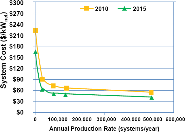
FIGURE F.11 Progression of fuel cell system costs with production volume.
SOURCE: James et al. (2010).
F.4.1.5 Onboard Hydrogen Storage: 2010
For onboard storage of hydrogen fuel, the physical storage of hydrogen as a compressed gas (35 or 70 MPa), has emerged as the technology path for the introduction of FCEVs (Hua et al., 2011; Jorgensen, 2011) because (1) it can release hydrogen at the required maximum rate and adjust to rapid changes in demand; (2) the time required to fill the tank is comparable to the time required to fill gasoline or diesel fueled vehicles; (3) energy losses during fueling, de-fueling, and long-term parking are minimal; and (4) compressed storage has been demonstrated in fleets of FCEVs.
The storage capacity, and hence the vehicle driving range, is limited by the volume and cost of tanks that can be packaged in vehicles. However, driving ranges over 300 miles are expected to be achieved. For example, in 2007 Toyota demonstrated a five-passenger FCEV with 70 MPa storage that traveled 350 miles in on-road conditions. Industry standards for fueling stations have been developed (e.g., SAE J2600 and J2601) and demonstrated at commercial public vehicle fueling stations offering hydrogen and gasoline pumps in the United States (Washington, D.C., California, and Michigan) and Germany (Munich, Frankfurt, and Berlin).
Carbon-fiber reinforced composite tanks have been employed to achieve sufficient strength for 70 MPa containment at manageable weight. Permeation is managed with an interior liner made either from a metal (e.g., aluminum) or a polymer (e.g., high-density polyethylene). Detailed cost analyses (Hua et al., 2011) show total system costs of $2,900 for representative 35 MPa systems (5.6 kg usable H2 stored; $15/kWh, $518/kg-H2) and $3,500 for 70 MPa systems (5.6 kg usable H2 stored; $19/kWh, $625/kg-H2) as shown in Figure F.12. Carbon fiber, priced at roughly $30/kg, accounts for most of the cost of the CFRC wrapped layers that provide the structural strength of the storage system. The remaining costs are primarily attributed to flow-regulating hardware.
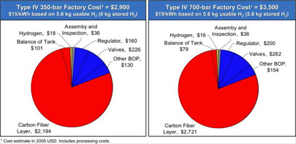
FIGURE F.12 Breakdown of compressed hydrogen storage system costs at high-volume production using 2010 technology.
SOURCE: Hua et al. (2011).
F.4.1.6 Vehicle Safety
The two primary features that distinguish FCEVs from conventional ICE vehicles with respect to safety are high-voltage electric power and hydrogen fuel. Safety of high-voltage electric power is managed on FCEVs similarly to HEVs, where safety requirements have resulted in on-road safety comparable to conventional ICE vehicles. Experience from decades of safe and extensive use of hydrogen in the agriculture and oil refining industries has been applied to vehicle safety and verified in vehicle maintenance and on-road demonstration programs. Fire risk is mitigated by the high dissipation rate of hydrogen, which is greater than gasoline fumes, and regulatory provisions for fuel system monitoring. Safety of high pressure onboard gaseous fuel storage has been demonstrated worldwide in decades of use in natural gas vehicles. Comparable safety criteria and engineering standards, as applied to ICEs, HEVs, and natural gas vehicles, have been applied to FCEVs (for example, Society of Automotive Engineers industry specifications: J1766, J2578, J2579, J2600, J2601, and J2719; and International Organization for Standardization specifications 14687-2, 15869, and 20100). The United Nations has drafted a Global Technical Regulation for hydrogen-fueled vehicles to provide the basis for globally harmonized vehicle safety regulations for adoption by member nations.
F.4.2 FCEV Cost and Efficiency Projections 2020-2050
F.4.2.1 2020-2030 Fuel Cell System Cost
Detailed analyses of current costs and expected technology advances that are already under demonstration have resulted in a fuel cell system cost estimate of $39/kW for a high-volume FCEV commercial introduction in 2015 (James et al., 2010). This estimate reflects recent advances in technology and material costs; for example, in both the cost and loading of precious metal in fuel cell
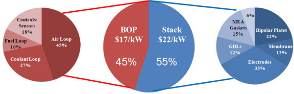
FIGURE F.13 Breakdown of fuel cell system costs at high-volume production using 2015 technology (stack power density 1000 mW/cm2 with 0.15 mg/cm2 Pt loading).
SOURCE: James et al. (2010).
electrodes. The platinum (Pt) loading in an earlier-generation stack with ~80 g Pt at $32/g (2005 Pt price) would cost ~$2,500. If only 10 g Pt were required in a higher-technology alloyed-Pt stack, the cost would be only ~$600, even at the higher 2011 Pt price of $58/g.
Figure F.13 shows the main sources of costs expected in 2015 for high-volume production. The total cost then is projected to be $39/kW. This report assumes $40/kW for the midrange in 2020. The optimistic case for 2020 is $36/kW, anticipating additional cost benefit from potential near-term technology developments, which are shown in Table F.29. All costing assumes commercial introduction of FCEVs at annual production volumes over 200,000 units, with the primary economy of scale occurring at 50,000 units (James et al., 2010).
Estimates for 2030 costs of fuel cell systems vary with optimism for the timing of technology advances currently under development. Projections of fuel cell system cost up to 2030 are linked to the achievement of technology advances already under development (see Table F.29, “Near-Term” and “Mid-Term”). An important and unique attribute of the automotive fuel cell system is the early stage in its development and application for on-road vehicles. Historically, gains in weight, volume, efficiency, and cost between successive early generations of a new technology are much more substantial than between more mature generations as early designs and materials are rapidly simplified, transformed and refined. Estimates of 2-3 percent per year reductions in high volume cost in early generations of a technology and 1 percent per year in later generations have commonly been observed (EPA, DOT, CARB, 2010). Therefore, for purposes of this report, technology-driven cost reduction from 2020 to 2030 of 2 percent per year is midrange, and 3 percent per year is optimistic. These advances are considerably less than the recent rate of fuel cell cost reduction (Figure F.10), because observed documented trends in technology cost apply to technologies that are market ready, not to technologies in a pre-commercial prototype stage of development. The technology-driven cost projections for fuel cell systems are summarized in Table F.30.
The fuel cell system costs are traditionally expressed as $/kW, because the change in cost of a system has generally been proportional to changes in vehicle power over the limited ranges of power currently used in FCEVs (James et al., 2010). However, significant deviation from a linear dependence of cost on net system power over a large range of vehicle power is expected for significant variations in vehicle power. This nonlinearity is difficult to project and is not included in cost estimation for this report. Nonlinearities are currently thought to be of secondary significance,52 but there is little experience or analysis to substantiate that assumption.
_____________________________
52 The committee received confidential input from vehicle manufacturers and suppliers.
TABLE F.29 Currently Recognized Opportunities for Technology Development for Improved Energy Efficiency and Cost
|
Near Term (2020) 1. Storage—reduced carbon fiber usage in storage systems—improved winding patterns 2. Storage—improved methods for tank production 3. Storage and fuel cell system—simplified design (fewer and cheaper components) 4. Storage and fuel cell system—improved manufacturing processes 5. Fuel cell system—reduced use of platinum (platinum alloys; new catalyst structures) 6. Fuel cell system—reduced transport losses by refined management of reactant flows and hydration and improved electrode structure 7. Fuel cell system—optimized stack and balance of plant (BOP) with optimized battery supplement for transient power 8. Fuel cell system—reduced BOP size and complexity from optimized reactant flow fields (for decreased stoichiometry and resultant lower mass flow rates) 9. Fuel cell system—reduced BOP size and complexity from membranes tolerant of lower humidity and/or higher temperature operation (simplified water management, lower pressure, and smaller radiator) 10. Fuel cell system—catalyst structures that increase and maintain the effective surface area of chemically active materials 11. Fuel cell system—higher temperature membranes for increased activity with less catalyst |
|
Mid-Term (2030) 1. Storage—reduced cost of carbon fiber—new production and processing methods 2. Storage—reduced carbon fiber usage in storage systems—smaller or lower-pressure vessels (associated with increased fuel cell system efficiency) 3. Storage—efficient low pressure cryo-storage 4. Fuel cell system—new durable membrane materials for low cost volume manufacture, thin design and low resistance 5. Fuel cell system—rapid manufacturing techniques for layered materials and for integration of layered materials into unit pieces for quick assembly 6. Fuel cell system—low cost, conductive, chemically stable plate materials 7. Storage and fuel cell system—capacity downsizing related to reduction in vehicle weight and increased efficiency of fuel cell system 8. Further progress in near-term opportunities |
|
Long Term (2050) 1. Fuel cell system—catalysts that do not use precious metals 2. Fuel cell system—capability for efficient operation at less than 1.2 stoichiometry 3. Fuel cell system—novel, low cost thermal management 5. Fuel cell system—refined designs for fluid flow in fuel cell stacks 6. Fuel cell system—new membrane materials and processing methods 7. Fuel cell system—novel processing techniques for catalyst substrates, impregnation and integration With layered materials 8. Storage—new low cost, high strength composite materials 9. Further progress in near-term and mid-term opportunities |
F.4.2.2 2050 Fuel Cell System Cost
Projections for 2050 shown in Table F.30 are based on technology achievements and refinements outlined in Table F.29 and on historical trends for cost improvement with advancing generations of mature technologies and manufacturing refinements (EPA, DOT, CARB, 2010). Historical trends include continuing technology advancement with further research and advances in new materials, analysis, simulation, and testing tools. Because of the expected major focus of fuel cell R&D on cost reduction prior to 2030, it is expected that subsequent cost reduction rates will not exceed norms for more mature generations of technologies (EPA, DOT, CARB, 2010). Therefore both midrange and optimistic cost estimates for 2050 include the 1 percent per year cost reduction rate associated with maturing technologies after 2030.
Evaluation of potential world Pt supply to support FCEVs as 50 percent of the on-road LDV sales by 2050 was conducted by TIAX (Carlson et al., 2003), assuming the conservative achievement of 15 g Pt per FCEV by 2050. Key documented findings are the following: (1) there are sufficient Pt resources in the ground to meet long-term projected Pt demand; (2) the Pt industry has the potential for expansion to meet demand for 50 percent market penetration of FCEVs (15 g Pt/vehicle) by 2050; and (3) the price of Pt may experience a short-term rise in response to increasing FCEV penetration, but is expected to return to its long-term mean once supply adjusts to demand. Scaled to 10 g Pt per FCEV (already achieved by 2010), the same conclusions apply to 80 percent penetration of the LDV sales by 2050.
F.4.2.3 2020-2050 Fuel Cell System Efficiency
Near-term technology developments for fuel cell systems are expected to be focused on reduction in fuel cell system cost without significant gain in fuel cell efficiency. Therefore, the midrange 2020 fuel cell system efficiency is taken to be 53 percent, which is equivalent to the 2010 estimated on-road fuel cell system efficiency. The optimistic 2020 fuel cell system efficiency is taken to be 55 percent, reflecting minimal expectation for efficiency gains while resources are focused on cost reduction. 55 percent is consistent with a minimal 0.5 percent per year improvement in the loss fraction over the nominal 2010 efficiency in the DOE demonstration fleet. Due to the primary focus on cost reduction, projections for both 2030 and 2050 midrange and optimistic efficiencies are expected to reflect only minimal 0.5 percent per year reduction in the loss fraction from the respective 2020 values. Fuel cell system efficiency projections are summarized in Table F.31.
TABLE F.30 Summary Fuel Cell System Cost Projections ($/kW)
| 2010 | 2020 | 2030 | 2050 | ||||||
| Midrange | 51 | 40 | 33 | 27 | |||||
| Optimistic | 51 | 36 | 27 | 22 | |||||
TABLE F.31 Summary of Fuel Cell Efficiency Projections
| 2010 | 2020 | 2030 | 2050 | ||||||
| Midrange | 53% | 53% | 55% | 60% | |||||
| Optimistic | 53% | 55% | 57% | 62% | |||||
F.4.2.4 2020-2030 Hydrogen Storage Cost
The cost of a CFRC hydrogen storage tank varies with the pressure and volume capacity. At present, nominal storage of 5.6 kg of 70 MPa hydrogen costs ~$3,500 (Hua et al., 2011). Reduction in the cost of tanks can be expected from new manufacturing/design techniques and smaller hydrogen storage systems. Storage systems get smaller as vehicle demand for fuel is reduced with improved vehicle efficiency (vehicle weight, aerodynamics, rolling resistance and powertrain efficiency).
Significant cost reduction from technology advancement within the 2010-2020 period is not expected due to current plans and capabilities of manufacturers for onboard storage.53 The midrange hydrogen storage cost for 2020 is derived from the 2010 estimated cost by scaling the system to contain the volume of hydrogen needed to maintain vehicle driving range with the vehicle efficiency projected for 2020. The scaling is accomplished by recognizing that roughly 75 percent of storage cost is proportional to the volume of stored hydrogen (variable cost); the remaining 25 percent of cost (boss and valve hardware) is not changed by the quantity of stored hydrogen (fixed cost is not sensitive to vehicle efficiency) (Hua et al., 2011). This assumes that a reduction in volume of stored hydrogen is accomplished by reducing tank size rather than eliminating a tank. This is consistent with consideration of packaging constraints for moderate reductions in vehicle demand. Dividing the cost into fixed and variable fractions is a means of approximating nonlinearities in the dependence of the storage system cost on its volumetric capacity when variations in that capacity are not small.
Estimates for midrange and optimistic 2030 technology-driven costs of hydrogen storage differ because of different estimates of the timing of technology advances currently under development (Warren, 2009) (Table F.29, “Near-Term” and “Mid-Term”). Several improvements in processing techniques have been identified (Warren, 2009) that are expected to reduce the cost of carbon fiber used in CFRC by 25 percent. That reduction is applied as a 1 percent per year midrange cost improvement from 2020 until 2040 to accommodate the technology development and its phased-in implementation into high-volume production. The 2030 optimistic cost projection assumes 2 percent per year technology-driven cost reduction from 2020 to 2030 in the variable cost fraction to accommodate full deployment of these new techniques for manufacture of carbon fiber by 2030.
However, less expensive manufacturing techniques are needed for producing carbon fiber from polyacrylonitrile or other precursor materials and for manufacturing storage tanks from the carbon fibers. Project success and commercialization of redesigned storage systems by 2030 are not certain but eventually could reduce storage costs significantly.
The fixed cost fraction, which is associated with flow-control equipment, is expected to have modest potential for cost reduction, because the technologies are mature. Therefore, a 1 percent per year cost reduction is applied to be consistent with historical improvements (EPA, DOT, CARB, 2010) in the design and materials used in mature technologies as they are applied in new areas, such as the 70 MPa compressed hydrogen application. The result is a projected 10 percent cost reduction in the fixed cost fraction over the 2020-2030 period.
In addition to these technology-related cost projections, additional reductions can be expected when the storage system is downsized—when the volume of hydrogen that needs to be stored for full vehicle range is reduced in response to increased vehicle efficiency. This reduction in the variable fraction of the storage cost is directly proportional to the reduced vehicle load. The difference between cost projections with and without downsizing of the storage system is illustrated by the difference between Tables F.32 and F.33.
_____________________________
53 The committee received confidential input from vehicle manufacturers and suppliers.
TABLE F.32 Technology-Driven Storage Cost Projections (constant 5.6 kg hydrogen capacity)
| 2010 | 2020 | 2030 | 2050 | ||||||
| Midrange | 5.6 | 5.6 | 5.6 | 5.6 | |||||
| Cost $ | 3,500 | 3,500 | 3,165 | 2,589 | |||||
| $/kg-H2 | 625 | 625 | 565 | 462 | |||||
| $/kWh | 19 | 19 | 17 | 14 | |||||
| Optimistic | |||||||||
| Cost $ | 3,500 | 3,500 | 2,936 | 2,232 | |||||
| $/kg-H2 | 625 | 625 | 524 | 399 | |||||
| $/kWh | 19 | 19 | 16 | 12 | |||||
TABLE F.33 Illustrative Hydrogen Storage System Cost Projectionsa from Technology Advances (Design, Material, and Manufacturing) and Reduced Size (Hydrogen Capacity)
| 2010 | 2020 | 2030 | 2050 | ||||||
| Midrange | |||||||||
| Capacity (kg) | 5.5 | 4.6 | 3.8 | 2.8 | |||||
| Cost ($) | 3,453 | 3,031 | 2,402 | 1,618 | |||||
| $/kg-H2 | 628 | 659 | 632 | 578 | |||||
| $/kWh | 19 | 20 | 19 | 17 | |||||
| Optimistic | |||||||||
| Capacity (kg) | 5.5 | 4.4 | 3.3 | 2.4 | |||||
| Cost ($) | 3,453 | 2,938 | 2,055 | 1,326 | |||||
| $/kg-H2 | 628 | 668 | 623 | 553 | |||||
| $/kWh | 19 | 20 | 19 | 16 | |||||
a Costs based on illustrative hydrogen storage capacity requirements.
F.4.2.5 2050 Hydrogen Storage System Cost
The midrange estimate for 2050 hydrogen storage cost results from continuation of the technology-driven 1 percent per year cost improvement over the 2030-2050 period in recognition of research into improvements in CRFC winding patterns54 and expectation of further improvements in manufacturing costs from added experience with high-volume production using new techniques (Warren, 2009). The result is an accumulated technology-driven cost reduction from 2020 to 2050 of 26 percent. As before, additional cost reductions result when the variable fraction of the storage system cost is scaled to accommodate the downsizing of storage associated with continually improving vehicle efficiency.
The optimistic estimate for 2050 hydrogen storage cost assumes a more aggressive technology-driven 2 percent per year cost improvement applied to the variable cost fraction for an additional 10-year
_____________________________
54 The committee received confidential input from vehicle manufacturers and suppliers.
period prior to 2050 in anticipation of aggressive research to reduce the cost of structural carbon or to find replacement materials or alternatives to compressed gaseous storage. Research on cost reduction of structural CFRC is expected to accelerate with the new market driver of its broadened application to airplane fuselages. And low pressure cryo-storage could become commercially viable.
Greater cost reductions are possible with manufacturing breakthroughs for carbon fiber, but that is not assumed here. However, it is noted that a reduction in storage cost associated with achievement of a targeted <$10/kg carbon fiber and pressure shift to 50 MPa would be consistent with a cost reduction of 35-40 percent, the optimistic technology-driven projection in Table F.32.
F.4.2.6 Trade-Offs with BEVs
FCEVs, like BEVs, are electric vehicles having no GHG emissions. Both are “fueled” by an energy carrier (electricity or hydrogen) that can be produced from a myriad of traditional and renewable energy sources (biofuels, natural gas, coal, and solar-, hydro-, and nuclear power). Three primary considerations differentiate their prospects for introduction and acceptance as LDVs: vehicle attributes, infrastructure, and rate of technology development.
• Vehicle attributes. FCEVs provide the full utility of current on-road vehicles. BEVs, however, require time consuming “refueling” (recharging) and only offer limited driving range between “refuelings.” In addition, FCEVs can be used to power a residence or business (or hydrogen fueling station) during electrical outages and, thereby, provide a form of back-up for the electrical grid, rather than the adding load for BEV recharging. Indeed, during an electrical outage caused by a winter storm, for example, a BEV could not be recharged to drive to a region with power and warm shelter.
• Infrastructure. FCEV commercialization will require the installation of hydrogen fueling pumps (with supporting onsite fuel storage and fueling equipment) at conventional fueling stations. In addition, a significant installation of regional facilities for production of hydrogen will be required. BEV commercialization requires installation of charging stations in homes or secure and accessible locations, upgrade of neighborhood transformers, and increase in electrical generating capacity for vehicle charging outside today’s off-peak hours. Infrastructure considerations are discussed further in Chapter 3 of this report. Long-term customer acceptance of in-home, near-home, and workplace/shopping charging installations remains to be established. Home chargers can be provided with individual vehicle sales, allowing vehicle manufacturers to somewhat decouple BEV sales from reliance on an independent deployment of infrastructure. However, FCEV sales will depend on the availability of hydrogen fueling stations and, hence, will require large-scale coordination of infrastructure and vehicle producers.
• Rate of technology development. A key requirement for realization of projected technology advances for battery and fuel cell systems is the continued dedication of R&D resources. Because demand for improved battery technologies is driven by their established application in portable communication/computer devices, prospects for short-term return on R&D investments are substantial.
In contrast, commercial application of fuel cell systems in vehicles is not seen as an outgrowth of communication/computer technologies. Instead, it depends on the likelihood of a substantial transition of the transportation sector to hydrogen fueled vehicles. The assessment of the prospects for such a transition likely depends on whether government energy policy signals a commitment to support deployment of hydrogen infrastructure and vehicles. Otherwise, the continued dedication of substantial private R&D resources to fuel cell vehicle technologies may not continue to support the current rate of progress in fuel cell technologies.
Projections of the timing and magnitude of improvements in efficiency and cost of fuel cell systems and the cost of hydrogen storage systems, as discussed in this chapter, are based on the fundamental assumption that resources—private and government—dedicated to R&D in support of fuel cell vehicles and hydrogen infrastructure are maintained at current levels or greater.
F.4.3 Cost and Performance Evolution of a Fuel Cell Electric Vehicle
As with BEVs, fuel cell vehicles currently are considerably more expensive than conventional ICEVs but have the potential to drop substantially in cost. The key factors in this expected cost reduction (aside from vehicle load reductions, which affect all vehicle regardless of drivetrain type) are expected improvements in efficiency and cost reductions in general electric drivetrain components (e.g., batteries and motors), expected strong increases in fuel cell efficiency, and strong expected cost reductions in fuel cell stacks and onboard storage costs. As shown in Table F.34, the overall effect of these factors will be to reduce vehicle costs by about $5,300-$6,600 by 2050, allowing fuel cell vehicles to have lower costs than their conventional ICE drivetrain competitors in 2050 (and possibly as early as 2030). Gasoline-equivalent fuel economy can range upwards of 170 mpg by 2050 and exceed 200 mpg in the optimistic case.
TABLE F.34 Details of the Potential Evolution of a Midsize Fuel Cell Vehicle, 2010-2050
| 2010 | 2030 mid | 2030 opt | 2050 mid | 2050 opt | |||||
| Fuel cell efficiency | 53 | 55.3 | 57.5 | 59.6 | 61.6 | ||||
| Fuel economy, test mpge | 94.1 | 125.8 | 149.5 | 170.4 | 211.3 | ||||
| Fuel cell power required, kW | 110.8 | 91.6 | 85.6 | 81 | 71.2 | ||||
| Hydrogen required for 390 mile (test) range, kg | 4.3 | 3.1 | 2.6 | 2.3 | 1.9 | ||||
| Fuel cell cost, $/kW | 50 | 33 | 27 | 27 | 22 | ||||
| Variable hydrogen tank cost, $/kg | 469 | 424 | 383 | 347 | 283 | ||||
| Incremental cost versus baseline, $ | 8,554 | 3,747 | 2,133 | 3,281 | 1,961 | ||||
| Incremental cost versus conventional, $ | 8,554 | 1,314 | –62 | –378 | –1,442 | ||||
F.5 REFERENCES
Aachen. 2010. Stiffness Relevance and Strength Relevance in Crash of Car Body Components. Conducted by the Institute fur Kraftfahrzeuge at the University of Aachen for the Aluminum Association. May 2010. Available at http://www.autoaluminum.org/downloads/NHTSAESV.6.2011.pdf.
Ballard Power Systems. 2006. CUTE: A Fuel Cell Bus Project for Europe Lessons Learned from a Fuel Cell Perspective. May 10 and 11. Available at http://cute-hamburg.motum.revorm.com/download/pdf/1/16.30%20CUTE%20Presentation%20-%20Geoff%20Budd.pdf.
Bandivadekar, A., .K. Bodek, L. Cheah, C. Evans, T. Groode, J. Heywood, E. Kasseris, M. Kromer, and M. Weiss. 2008. On the Road in 2035—Reducing Transportation’s Petroleum Consumption and Greenhouse Consumption. Available at http://web.mit.edu/sloan-auto-lab/research/beforeh2/otr2035/On%20the%20Road%20in%202035_MIT_July%202008.pdf.
BMW. 2009. “Thermoelectric Power Generation—The Next Step to Future CO2 Reductions?!” Presentation by A. Eder, BMW Efficient Dynamics/Thermal Management, at the 2009 Thermoelectrics Applications Workshop on September 30. Available at http://www1.eere.energy.gov/vehiclesandfuels/pdfs/thermoelectrics_app_2009/wednesday/eder.pdf.
Carlson, E.J., M. Greenfield, Y. Huang, M. Noordzij, T. Rhodes, and J. Yurko, TIAX, LLC. 2003. Platinum Availability and Economics for PEMFC Commercialization. Subcontract Report. National Renewable Energy Laboratory. December. Summary slides available at http://www1.eere.energy.gov/hydrogenandfuelcells/pdfs/tiax_platinum.pdf.
Carlson, E.J., P. Kopf, J. Sinha, and S. Sriramulu. 2005. Cost Analysis of PEM Fuel Cell Systems for Transportation. Subcontract Report NREL/SR-560-39104. National Renewable Energy Laboratory. U.S. Department of Energy. September 30.
Carpenter, Jr., J., U.S. Department of Energy. 2008. “Challenges to Automotive Composites.” Presentation to the American Chemistry Council, Plastics Division, Arlington, Va., May 20. Washington, D.C.
DOT (Department of Transportation). 2011. ITS Strategic Research Plan. Washington, D.C.: U.S. Department of Transportation, Research and Innovative Technology Administration. June. Available at via http://www.rita.dot.gov.
EPA (Environmental Protection Agency). 2010a. Final Rulemaking to Establish Light-Duty Vehicle Greenhouse Gas Emission Standards and Corporate Average Fuel Economy Standards, Regulatory Impact Analysis. Washington, D.C. April. Available at http://epa.gov/oms/climate/regulations/420r10009.pdf.
———. 2010b. Light-Duty Automotive Technology, Carbon Dioxide Emissions, and Fuel Economy Trends: 1975 Through 2010. EPA-420-R-10-023. Compliance and Innovative Strategies Division and Transportation and Climate Division, Office of Transportation and Air Quality. November. Available at http://www.epa.gov/oms/cert/mpg/fetrends/420r10023.pdf.
EPA, DOT, CARB (California Air Resources Board). 2010. Light-Duty Vehicle Greenhouse Gas Emission Standards and Corporate Average Fuel Economy Standards for Model Years 2017-2025. Interim Joint Technical Assessment Report. Available at http://www.epa.gov/oms/climate/regulations/ldv-ghg-tar.pdf.
EPA, NHTSA (National Highway Traffic Safety Administration), CARB. 2010. Interim Joint Technical Assessment Report: Light-Duty Vehicle Greenhouse Gas Emission Standards and Corporate Average Fuel Economy Standards for Model Years 2017-2025. Washington, D.C.
FEV (FEV, Inc.). 2012. FEV, Light-Duty Vehicle Technology Cost Analysis—European Vehicle Market (Phase 1). Analysis Report BAV 10-449-001. Prepared for the International Council on Clean Transportation.
Ford (Ford Motor Company). 2012. Bill Ford Outlines “Blueprint for Mobility” Vision; Calls on Mobile Industry to Help Develop Transportation Solutions. Press Release. Available at http://media.ford.com.
Gibbs, W.W. (2006). Innovations from a robot rally. Scientific American, January. Available at http://www.scientificamerican.com/article.cfm?id=innovations-from-a-robot-2006-01&sc=I100322.
Hua, T., R. Ahluwalia, J. Peng, M. Kromer, S. Lasher, K. McKenney, K. Law, and J. Sinha. 2011. Technical assessment of compressed hydrogen storage tank systems for automotive applications. International Journal of Hydrogen Energy 36(4):3037-3049.
IBIS (IBIS Associates, Inc.). 2008. Aluminum Vehicle Structure: Manufacturing and Lifecycle Cost Analysis Hybrid Drive and Diesel Fuel Vehicles. Report by IBIS Associates for The Aluminum Association. May 2008. Available at http://www.drivealuminum.org/research-resources/documents/2008-ibis-powertrain-study.
James, B.D., J.A. Kalinoski, and K.N. Baum. 2010. Mass Production Cost Estimation for Direct H2 PEM Fuel Cell Systems for Automotive Applications: 2010 Update. NREL Report No. SR-5600-49933. Directed Technologies, Inc. Available at http://www1.eere.energy.gov/hydrogenandfuelcells/pdfs/dti_80kwW_fc_system_cost_analysis_report_2010.pdf. (Summary slides, B.D. James, J.A. Kalinoski, and K.N. Baum, Mass-Production Cost Estimation for Automotive Fuel Cell Systems, DOE H2 Program Review 2010, available at http://www.hydrogen.energy.gov/pdfs/review10/fc018_james_2010_o_web.pdf).
Jorgensen, S. 2011. Hydrogen storage tanks for vehicles: Recent progress and current status. Current Opinion in Solid State and Materials Science 15:39-43.
Kahane, C. 2011. Relationships Between Fatality Risk, Mass, and Footprint in Model Year 2000-2007 Passenger Cars and LTVs. NHTSA. Available at http://www-nrd.nhtsa.dot.gov/Pubs/811665.pdf.
Kromer, M.A., and J.B. Heywood. 2007. Electric Powertrains: Opportunities and Challenges in the U.S. Light-Duty Vehicle Fleet. MIT publication LFEE 2007-02 RP. Available at http://web.mit.edu/sloan-auto-lab/research/beforeh2/files/kromer_electric_powertrains.pdf.
Lotus. 2010. An Assessment of Mass Reduction Opportunities for a 2017-2020 Model Year Vehicle Program. Report submitted to the International Council on Clean Transportation. March. Available at http://theicct.org/lotus-lightweighting-study.
Markoff, J. 2010. Google cars drive themselves, in traffic. The New York Times, October 9. Available at http://www.nytimes.com/2010/10/10/science/10google.html.
Mitchell, W.J., C.E. Borroni-Bird, and L.D. Burns. (2010). Reinventing the Automobile: Personal Urban Mobility for the 21st Century. Cambridge, Mass.: MIT Press.
NHTSA (National Highway Traffic Safety Administration). 2010. Corporate Average Fuel Economy for MY 2012-MY 2016 Passenger Cars and Light Trucks, Final Regulatory Impact Analysis. March. Available at http://www.nhtsa.gov/staticfiles/.../CAFE_2012-2016_FRIA_04012010.pdf.
NHTSA, EPA. 2010. 2017-2025 Model Year Light-Duty Vehicle GHG Emissions and CAFE Standards: Supplemental Notice of Intent. Report EPA-HQ-OAR-2010-0799; NHTSA-2010-0131] RIN 2060-AQ54; RIN 2127-AK79.
———. 2010b. Interim Joint Technical Assessment Report: Light-Duty Vehicle Greenhouse Gas Emission Standards and Corporate Average Fuel Economy Standards for Model Years 2017- 2025. September 2010. Available at http://www.epa.gov/oms/climate/regulations/ldv-ghg-tar.pdf
———. 2011. 2017 and Later Model Year Light-Duty Vehicle Greenhouse Gas Emissions and Corporate Average Fuel Economy Standards Proposed Rule. November. Available at https://www.federalregister.gov/articles/2012/01/13/2012-617/2017-and-later-model-year-light-duty-vehicle-greenhouse-gas-emissions-and-corporate-average-fuel.
NRC (National Research Council). 2001. Review of the Research Program of the Partnership for a New Generation of Vehicles: Seventh Report (plus earlier reports in the series). Washington, D.C.: National Academy Press.
———. 2005. Review of the Research Program of the FreedomCAR and Fuel Partnership. Washington, D.C.: The National Academies Press.
———. 2006. Tires and Passenger Vehicle Fuel Economy—Informing Consumers, Improving Performance. Transportation Research Board Special Report 286. Washington, D.C.: The National Academies Press.
———. 2008. Transitions to Alternative Transportation Technologies—A Focus on Hydrogen. Washington, D.C.: The National Academies Press.
———. 2010. Technologies and Approaches to Reducing the Fuel Consumption of Medium-and Heavy-Duty Vehicles. Washington, D.C.: The National Academies Press.
———. 2011. Assessment of Fuel Economy Technologies for Light-Duty Vehicles. [Sometimes referred to as the “2010 NAS CAFE report.”] Washington, D.C.: The National Academies Press.
ORNL (Oak Ridge National Laboratory). 2008. “Future Lower Cost Carbon Fiber for Autos: International Scale-up & What is Needed.” Presentation by C. David Warren, ORNL, to the SPEA Automotive Conference. Available at http://www.speautomotive.com/SPEA_CD/SPEA2008/pdf/k/K2.pdf.
Osram Sylvania. 2011. Automotive Solid State Lighting. Press Release. D. Hulik. January 24. Available at http://www.engadget.com/2011/01/24/led-headlights-can-add-up-to-six-miles-of-electric-vehicle-range/.
Powers, W. 2000. Automotive materials in the 21st century. Advanced Materials and Processes, May.
Reuters. 2012. Toyota Finds Way to Avoid Using Rare Earth: Report. Available at http://www.reuters.com/article/2012/01/23/us-toyota-rare-earth-idUSTRE80M0JK20120123. Accessed August 1, 2012.
Ricardo (Ricardo, Inc.). 2008. A Study of Potential Effectiveness of Carbon Dioxide Reducing Vehicle Technologies. USEPA 420-R-08-004. Prepared for EPA by Ricardo, Inc. Available at http://nepis.epa.gov/EPA/html/DLwait.htm?url=/Exe/ZyPDF.cgi?Dockey=P1001TUM.pdf.
———. 2011. Report to the Aluminum Association. Summary available at http://www.autoaluminum.org/downloads/info_kit/2011EV.pdf.
Rugh, J.P., Chaney, L., Lustbader, J., Meyey, J., Rustagi, M., Olson, K., Kogler, R. 2007. Reduction in Vehicle Temperatures and Fuel Use from Cabin Ventilation, Solar-Reflective Paint, and a New Solar-Reflective Glazing. Technical Paper SAE 2007-01-1194. SAE International, Warrendale, Pa.
Vanderbilt, T. 2012. Let the robot drive: The autonomous car of the future is here. Wired Magazine. Issue 20.02. February. Available at http://www.wired.com/magazine/2012/01/ff_autonomouscars/.
Warren, C.D. 2009. Carbon Fiber Technology Development, ORNL presentation report. Available at http://www.ornl.gov/sci/physical_sciences_directorate/mst/PMC/carbon_fiber09/index.html.
Wipke, K., S. Sprik, J. Kurtz, and T. Ramsden. 2010a. 2010 Annual Progress Report for NREL’s Controlled Hydrogen Fleet and Infrastructure Analysis Project, Section VII.1. Available at http://www.nrel.gov/hydrogen/pdfs/viii_controlled_fleet.pdf.
———. 2010b. Controlled Hydrogen Fleet and Infrastructure Demonstration and Validation Project, Fall 2010. NREL Report No. TP-5600-49642. Available at http://www.nrel.gov/hydrogen/pdfs/49642.pdf.


