
G.1 RENEWABLE FUEL STANDARD
The federal Renewable Fuel Standard (RFS) was created under the Energy Policy Act of 2005 because Congress recognized “the need for a diversified portfolio of substantially increased quantities of … transportation fuels” to enhance energy independence (P.L. 109-58). RFS required an increase use of renewable fuels from 4.0 billion gallons per year in 2006 to 7.5 billion gallons in 2012 (Figure G.1). Because what constitutes “renewable” is determined by a set of legal definitions, the RFS was designed to encourage the consumption of a specific type of non-petroleum based alternative fuel (that is, biofuels). The U.S. biofuel consumption from 2006 to 2008 exceeded the RFS consumption mandates.
The Energy Independence and Security Act of 2007 (EISA 2007) was enacted “to move the United States toward greater energy independence and security” and to “increase the production of clean renewable fuels.” EISA 2007 amended the RFS, creating what is referred to as RFS2 by modifying the program in several key ways:
• It expanded the RFS program to include diesel, in addition to gasoline, produced in or imported into the United States;
• The amendment extended the time horizon to 2022.
• The incremental volumes of renewable fuel required to be consumed have increased to 10.6 billion gallons of ethanol equivalent fuels plus 0.5 billion gallons of biomass-based diesel in 2008 and 35 billion gallons of ethanol equivalent plus 1 billion gallon of biomass-based diesel in 2022;
• It established four categories of renewable fuel based on the feedstock source and on life-cycle GHG emission thresholds. There are separate volume requirements for each one (Figure G.1).
The four renewable fuel categories are nested within the mandate and are differentiated by the reduction in life-cycle greenhouse gas (GHG) emissions using the methodology developed by U.S. Environmental Protection Agency (EPA; Federal Register 40 CFR part 80, p. 14669) and include indirect land-use changes distributed over the expected 30 year life of the biofuel refineries. The four categories are (Figure G.1) as follows:
• Conventional biofuels, usually ethanol derived from starch of corn grain (corn-grain ethanol). Conventional biofuel produced from facilities that commenced construction after December 19, 2007, would have to achieve at least a 20 percent reduction in life-cycle GHG emissions compared to petroleum-based gasoline and diesel to qualify as a renewable fuel under RFS2. The quantities are measured in terms of ethanol equivalent gallons.
• Advanced biofuels, which are renewable fuels other than corn-grain ethanol, achieve at least a 50 percent reduction in life-cycle GHG emissions. Advanced biofuels can include ethanol and other types of biofuels derived from such renewable biomass as cellulose, hemicellulose, lignin, sugar, or any other
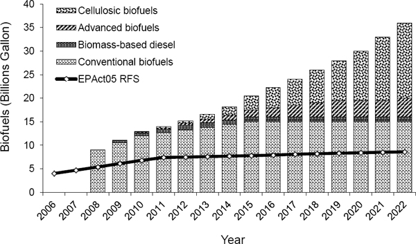
FIGURE G.1 Mandated consumption target for different categories of biofuels under the Energy Independence and Security Act of 2007.
NOTE: The line shows the consumption target under the Energy Policy Act of 2005 (EPAct05 RFS).
SOURCE: NRC (2011).
starch that is not from corn, biomass-based diesel, and coprocessed renewable diesel.1 The mandate requires 4 billion gallons per year of advanced biofuels measured in terms of ethanol equivalent gallons in 2022.
• Cellulosic biofuels are renewable fuels derived from any cellulose, hemicellulose, or lignin from renewable biomass that achieve at least a 60 percent reduction in life-cycle GHG emissions. In general, cellulosic biofuels also qualify as renewable fuels and advanced biofuels. The mandate requires 16 billion gallons per year of cellulosic biofuels measured in terms of ethanol equivalent gallons in 2022.
• Biomass-based diesel, including biodiesel2 made from vegetable oils or animal fats and cellulosic diesel, achieves at least a 50 percent reduction in life-cycle GHG emissions—for example, soybean biodiesel and algal biodiesel. Co-processed renewable diesel is excluded from this category. The mandate currently requires 1 billion gallons per year of biodiesel expressed as gallons of methyl ester-based biodiesel energy equivalents.
While corn-grain ethanol is only allowed to fulfill the conventional biofuels volume, biofuels from other categories could also fill the conventional biofuels volume if cellulosic biofuels become less expensive than corn-grain ethanol. There is not a specific mandate for corn-grain ethanol.
RFS2 also defines the energy equivalence of various biofuels relative to ethanol. One gallon of biodiesel is worth 1.5 gallons of ethanol. One gallon of renewable diesel3 is worth 1.7 gallons of ethanol. One gallon of biobutanol is worth 1.3 gallons of ethanol. Other fuels are rated by petition to EPA based
_____________________________
1 Co-processed renewable diesel refers to diesel made from renewable material mixed with petroleum during the hydrotreating process.
2 Biodiesel is a diesel fuel consisting of long-chain alkyl esters derived from biological materials such as vegetable oils, animal fats, and algal oils.
3 Renewable diesel is they hydrogenation product of triglcerides derived from biological materials.
on their energy content relative to ethanol. Therefore, the mandate can be met with lower volumes of fuels with higher energy contents.
RFS2 requires that all renewable fuels be made from feedstocks that meet a new definition of renewable biomass. In EISA 2007, the definition of renewable biomass incorporates land restrictions for planted crops, crop residue, planted trees and tree residue, slash and precommercial thinnings, and biomass from wildfire areas. Detailed definitions and EPA’s interpretations of the terms are found in Regulation of Fuels and Fuel Additives: Changes to Renewable Fuel Standard Program; Final Rule (EPA, 2010a: pp. 14691-14697). A brief version of EISA’s renewable biomass definition and land restrictions is includes the following:
• Planted crops or crop residues that were cultivated at any time prior to December 19, 2007, on land that is either actively managed or fallow and nonforested.
• Planted trees and tree residue from actively managed tree plantations on non-federal land cleared at any time prior to December 19, 2007, including land belonging to an Indian tribe or an Indian individual, which is held in trust by the United States or subject to a restriction against alienation imposed by the United States.
• Slash and precommercial thinnings from non-federal forestlands, including forestlands belonging to an Indian tribe or an Indian individual, that are held in trust by the United States or subject to a restriction against alienation imposed by the United States.
• Biomass obtained from the immediate vicinity of buildings and other areas regularly occupied by people, or of public infrastructure, at risk from wildfire.
• Algae.
G.2 INFRASTRUCTURE INITIAL INVESTMENT COST
As shown in Chapter 3, the investment cost per gallon of gasoline equivalent (gge) per day to build the fuel infrastructure is sizable for all of the alternate fuel and vehicle pathways. Table G.1 shows this cost in 2030 for each fuel expressed in the cost per gge/day, or in the case of electricity cost per kilowatt-hour per day. The costs shown in Table G.1 reflect only the investment costs that involve building a new form of infrastructure needed to use the fuel as a transportation fuel, not those for expanding an already large and functioning infrastructure associated with its more traditional use.
• Electricity. Home charger and public charger costs are included. Expansions of producing, transmitting, and distributing electricity and expansions to produce more of the base fuel are not (natural gas, coal, wind, and solar) are not included. A cost for a parking space for access to charging also is not included.
• Hydrogen. Costs to convert the base fuel (natural gas, coal, biomass or electricity) to hydrogen are included, carbon capture and storage (CCS) is included when used, and costs to distribute and to deliver hydrogen to the vehicle are included. Expansions to produce more of the base fuel are not included.
• Natural gas. Costs for new natural gas stations to deliver this fuel to a vehicle are included. Expansions of the natural gas producing and transmission system are not included.
• GTL. Costs to convert natural gas to gasoline are included. Expansions of the natural gas producing and transmission system and the gasoline station costs are not included.
• CTL. Costs to convert coal to gasoline are included. CCS is included. Expansions of the coal producing and delivery system and the gasoline station costs are not included.
• Biofuels. Costs to convert biomass to liquid fuels are included. Expansions of the biomass growing, collecting and delivery systems and the gasoline station costs are not.
• Gasoline (new plant). New refinery cost to convert crude oil to gasoline are included for comparison. Costs of producing crude oil and gasoline station costs are not.
The overall infrastructure investment needs for a vehicle using any of the fuels in Table G.1 is found by multiplying this investment cost by the fuel (gge) consumed per day. Using 13,000 miles per year for all vehicles, 4.0 miles per kilowatt-hour (kWh) for electric vehicles (EVs), 80 miles/gge for HFCVs, and 40 miles/gge for liquid fuel vehicles to reflect approximate 2030 mileage rates shown in the Chapter 5 Reference Case, the investment costs per vehicle are shown in Tables G.2 and G.3.
G.3 POLICY AREAS TO BE ADDRESSED TO INCREASE THE SHARE OF ALTERNATIVE FUELS USED IN LIGHT-DUTY VEHICLES
From the fuels perspective, policy areas where actions are required to progress along the path of research and development, demonstration, deployment, and rapid growth for each of the alternate fuels. Policy actions need to address, in an effective manner, each of the areas marked with an X or the fuel pathway is unlikely to grow to maturity with production in low-GHG methods (Table G.4).
G.4 POTENTIAL AVAILABILITY OF BIOMASS FOR FUELS
Several potential sources of non-food biomass can be used to produce biofuels. They include crop residues such as corn stover and wheat straw, fast-growing perennial grasses such as switchgrass and Miscanthus, whole trees and wood waste, municipal solid waste, and algae. Each potential source has a production limit.
Several studies have been published on the estimated the amount of biomass that can be sustainably produced in the United States. All of the studies focused on meeting particular production goals, and none of them project biomass availability beyond 2030. For example, the objective of the report Biomass as Feedstock for a Bioenergy and Bioproducts Industry: The Technical Feasibility of a Billion-Ton Annual Supply (commonly referred to as the “billion-ton study”) was to determine the feasibility of producing sufficient biomass to reduce petroleum consumption by 30 percent (Perlack et al., 2005). That study estimated that 1 billion tons of biomass would be needed to displace 30 percent of the U.S. petroleum consumption in 2005. The four studies that were analyzed in the report Renewable Fuel Standard: Potential Economic and Environmental Effects of U.S. Biofuel Policy (NRC, 2011) focused on the feasibility of producing sufficient biomass to meet the RFS2 mandates in 2022. All those studies concluded that sufficient RFS-compliant biomass would be available to produce biofuels for meeting the consumption mandate. None of these studies attempted to estimate the maximum production rates that could be attained if the RFS2 biomass restrictions were eliminated or if different economic assumptions, such as a carbon tax, were made.
The 2009 report Liquid Transportation Fuels from Coal and Biomass: Technological Status, Costs, and Environmental Impacts (NAS-NAE-NRC, 2009) evaluated the role of biofuels in America’s energy future. The panel assessed the potential availability of biomass feedstock that would not incur competition for land with crops or pasture and for which the environmental impact of biomass production for biofuels was no worse than the original land use. They concluded that 550 million dry tons of cellulosic feedstock could be sustainably produced for biofuels in 2020. The billion-ton study (Perlack et al., 2005) was recently updated and the U.S. Billion Ton Update was released in 2011 (DOE, 2011). As in the first study, its objective was to estimate if 1 billion tons of biomass could be sustainably and economically produced in the lower 48 states by the year 2030. Projections beyond 2030 were not made, and the study did not attempt to estimate maximum biomass that could be harvested. The updated study defined “economic production” as all material that could be produced at or below a farm-gate price of $60/dry ton. This is not an average biorefinery feedstock price, but is a maximum price at the farm or
TABLE G.1 2030 Fuel Infrastructure Investment Costs, $/gge per day
| Alternate Fuel | 2030 Investment Cost, $/kWh per day or $/gge per day |
| Electricity (PHEV-10) | 370 $/kWh per day |
| Electricity (PHEV-40) | 530 $/kWh per day |
| Electricity BEV | 330 $/kWh per day |
| Hydrogen (with CCS) | 3,890 $/gge per day |
| Natural gas (CNG) | 910 $/gge per day |
| GTL | 1,900 $/gge per day |
| CTL/CCS | 2,500 $/gge per day |
| Biofuel (thermochemical) | 3,100 $/gge per day |
| Gasoline (new plant—if needed) | 595 $/gge per day |
TABLE G.2 2030 Fuel Infrastructure Investment Costs per Vehicle
| Alternate Fuel | Fuel Use/Day, kWh/day or gge/day | Infrastructure Investment Cost per Vehicle, $ |
| Electricity (PHEV-10) | 1.75 kWh/day | $650 |
| Electricity (PHEV-40) | 5.4 kWh/day | $2,880 |
| Electricity BEV | 8.92 kWh/day | $2,930 |
| Hydrogen (with CCS) | 0.45 gge/day | $1,370 |
| Natural gas (CNG) | 0.89 gge/day | $810 |
| GTL | 0.89 gge/day | $1,690 |
| CTL | 0.89 gge/day | $2,220 |
| Biofuel (thermochemical) | 0.89 gge/day | $2,760 |
| Gasoline (new plant—if needed) | 0.89 gge/day | $530 |
TABLE G.3 2030 Fuel Infrastructure Investment Costs per Vehicle—Highest to Lowest
| Alternate Fuel | 2030 Investment Cost, $/gge per day or $/kWh per day | Car Fuel Use/Day, gge/day or kWh/day | Infrastructure Investment Cost, $/Vehicle | ||||||
| Electricity BEV | 330 $/kWh per day | 8.92 kWh/day | $2,930 | ||||||
| Electricity (PHEV-40) | 530 $/kWh per day | 5.45 kWh/day | $2,880 | ||||||
| Biofuel (thermochemical) | 3,100 $/gge per day | 0.89 gge/day | $2,760 | ||||||
| CTL | 2,500 $/gge per day | 0.89 gge/day | $2,220 | ||||||
| Hydrogen (with CCS) | 3,890 $/gge per day | 0.45 gge/day | $1,750 | ||||||
| GTL | 1,900 $/gge per day | 0.89 gge/day | $1,690 | ||||||
| Natural gas (CNG) | 910 $/gge per day | 0.89 gge/day | $810 | ||||||
| Electricity (PHEV-10) | 370 $/kWh per day | 1.75 kWh/day | $650 | ||||||
| Gasoline (new plant—if needed) | 595 $/gge per day | 0.89 gge/day | $530 | ||||||
TABLE G.4 Policies Areas to be Addressed to Increase the Share of Alternative Fuels Used in Light-Duty Vehicles
| Biofuels | Electricity for PHEVs | Hydrogen | CNG | GTL | CTL/CCS | |
| Consistent RD&D support to advance technology development and lower costs. | X | Xa | Xb | X | X | |
| Actions to facilitate demonstration of new fuels technology at small commercial scale. | X | Xc | ||||
| Actions to ensure continued research, development, demonstration and deployment of CCS.d | X | X | X | |||
| Actions to encourage the initial deployment of the fuel infrastructure to coincide with vehicle introductions and early growth. | Xe | Xf | Xg | X | ||
| Actions to reduce the consumer price of alternate fuels at the beginning of a transition to encourage the use in existing vehicles or new vehicle types. | Xh | X | X | X | ||
| Following successful fuel/vehicle introductions, when large quantities of fuel are needed, actions that limit GHGs associated with producing the fuel. | Xi | X | X |
a DOE funding has not been consistent.
b DOE funding has not been consistent, but the new Advanced Research Projects Agency-Energy program is beginning.
c Small demonstrations have been made but not at nearly commercial scale.
d Research and development is being done but commercial viability is not yet demonstrated.
e RFS2 addresses this issue.
f Programs to install public chargers in some locations. May need to be expanded.
g California is addressing this through mandated station construction.
h RFS2 addresses this issue.
i RFS2 addresses this issue.
forest gate. At least a portion of the biomass production would be available at a lower cost. The cost to produce biofuels based on a feedstock price of $75 to $133 per dry ton at the refinery gate is discussed later in this appendix. Two scenarios were evaluated at the price ceiling of $60 in the U.S. Billion-Ton Update : a baseline case that assumed an annual crop yield growth of 1 percent and a high crop yield case that assumed a 2 to 4 percent annual yield improvement in commodity crops and energy crops. The study also accounted for biomass that was currently being used to produce energy. The projected availabilities of biomass for fuels from the two studies are summarized in Figure G.2.
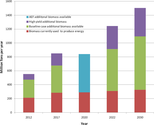
FIGURE G.2 Biomass availability estimates from the U.S. Billion-Ton Update (DOE, 2011) from the report Liquid Fuels for Transportation from Coal and Biomass: Technological Status, Costs, and Environmental Impacts (NAS-NAE-NRC, 2009). NOTE: Data for years 2012, 2017, 2022, and 2030 are from DOE (2011) and the estimated biomass availability for biofuel production from NAS-NAE-NRC (2009) for the year 2022 is added on top of the biomass projected to be used for electricity generation.
The estimate in the NAS-NAE-NRC report (2009) is consistent with the billion-ton study baseline case when interpolated to the same year. If the billion-ton study baseline case (which includes a 1 percent annual increase in biomass productivity) is linearly extrapolated to 2050, then 1350 million tons of additional biomass (above that currently used for energy production) are projected to be available to produce biofuels in 2050.
U.S. Billion-Ton Update (DOE, 2011) primarily analyzed biomass production from energy crops and forest and agricultural residue recovery. Its estimate of biomass availability for cellulosic biofuels in 2022 is comparable to the 550 million dry tons that the NAS-NAE-NRC (2009) report estimated for 2020. By 2030, the baseline case of the study (which includes a 1 percent annual yield growth) concluded that an additional 767 million dry tons of biomass would be available at prices of less than $60 per ton. The production of additional biomass would require a shift of 22 million acres of cropland and 41 million acres of pasture land into energy crop production by 2030. That report concluded that at $60 per ton, none of the existing wood products would be diverted to fuel production. At higher prices, however, some pulpwood and lumber would begin to be diverted to fuel use.
There is other evidence, however, that a substantial amount of forest biomass could be utilized for biofuels production. With the economic downturn, a decrease of almost a 100 million dry ton per year in U.S. wood production (harvest) was observed between 2008 and 2010 (Figure G.3). This additional forest biomass was not included in the billion-ton study projections.
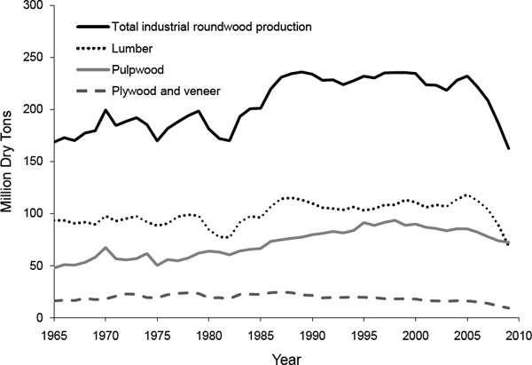
FIGURE G.3 U.S. industrial wood production.
DATA SOURCE: Howard (2007); updated data to 2009 as result of personal communication.
FIGURE SOURCE: NRC (2011).
Annual removals from U.S. forestlands, including roundwood products, logging residues, and other removals from growing stock and other sources, were estimated to be about 21.2 billion cubic feet annually, which is about 320 million dry tons of biomass. This level of harvest is well below net annual forest growth and only a small fraction of the total timberland inventory (Figure G.4). In 2006, the ratio of forest-growing stock growth (wood volume increases) to growing stock removals (for example, harvest and land clearing) in the United States was 1.71, which indicates that net forest growth exceeded removals by 71 percent (Smith et al., 2009). The 320 million dry ton removal does not match the wood production, because part of the total wood removal is residue that is being used to produce energy. Because about 320 million dry tons per year are being produced each year and forest mass is increasing at a ratio of 1.71, based on 2007 harvest rates, an additional 225 million tons per year could be removed. If harvest rates in 2012 were at least 75 million tons lower than that in 2007, a total of over 300 million tons of forest biomass would be available sustainably with no land-use change.
Many estimates of potential biomass availability have been made, but to accurately predict how much biomass will actually be supplied for biofuel production at any future date is extremely difficult. There appears to be consensus among studies that sufficient biomass could be produced to meet the 2022 RFS2 consumption mandate). Meeting the RFS2 mandate will require an additional 200-300 million dry tons per year of biomass.
Another source of biomass for fuel is microalgae and cyanobacteria (DOE, 2010b; Singh and Gu, 2010). Microalgae are produced commercially as nutritional supplements and for cosmetics (Spolaore et al., 2006; Earthrise, 2009). Many companies are pursuing the commercial production of algal biofuels (USDA-RD, 2009; DOE, 2010a,b). At present, algal biofuels are further from commercial deployment than cellulosic biofuels, and their costs have been estimated to be $10-$20 per gallon of diesel (Davis et al., 2011). Therefore, algal biofuels are not considered in this detail in this report.
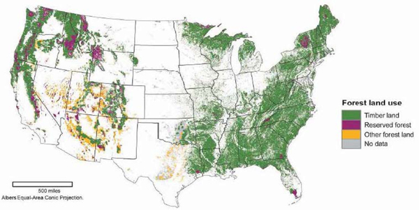
FIGURE G.4 Forest resources of the United States. In the United States, there are about 750 million acres of forestland, with slightly more than two-thirds classified as timberland or land capable of producing 20 cubic feet per acre annually of industrial wood products in natural stands (Smith et al., 2009). Another 22% of this forestland is classified as “other” and is generally not productive enough for commercial timber operations owing to poor soils, lack of moisture, high elevation, or rockiness. The remaining 10% of forestland is withdrawn from timber utilization by statute or administrative regulations and is dedicated to a variety of non-timber uses, such as parks and wilderness. The timberland fraction of U.S. forestlands totals approximately 514 million acres. As noted by Smith et al. (2009), the map above shows forested pixels from the USDA Forest Service map of Forest Type Groups (Ruefenacht et al., 2008). Timberland is derived and summarized from RPA plot data using a hexagon sampling array developed by EPA. Reserved land is derived from the Conservation Biology Institute, Protected Areas Database. Other forestland is non-timberland forests.
SOURCE: DOE (2011 p. 18).
G.5 ESTIMATING GREENHOUSE-GAS EMISSION IMPACTS OF BIOFUELS
Ascertaining the net GHG emission impact of biofuels is challenging because of the complexities in fully characterizing the GHG effects associated with the supply chain and management practices and the interactions with real-world markets for commodities and land. Attributional life-cycle assessment (LCA) calculations based on direct emissions generally find that, if efficiently produced, biofuels have a lower GHG emission impact than the fossil fuels they replace. However, the adequacy of an attributional LCA for reliably assessing the GHG impacts of fuels is being called into question, with GHG emission effects from land-use changes being a major area of uncertainty. Complex LCA calculations, including estimated changes in land use induced by increasing use of biomass as an energy source, have shown variable results because of different assumptions on the magnitude of the changes, the amount of GHG emitted, and the time frame considered. (See for example, the Renewable Fuel Standard Program (RFS2) Regulatory Impact Analysis; EPA, 2010b).
Direct land-use changes can be estimated based on land area that would have to be converted from some other use to grow a given amount of biomass. For this analysis, three types of cellulosic biomass are assumed to be harvested or grown in the United States for biofuel production: crop residue (mostly corn stover), woody biomass, and switchgrass (to represent high-yield perennial grasses). The production of crop residue and woody biomass is assumed to be scaled up with little if any net GHG
BOX G.1 Examples of Indirect Land-Use Changes from Increasing Biofuel Production
Domestic
Increased corn production in the Midwest to supply ethanol production could induce the withdrawal of land from the Conservation Reserve Program to grow wheat that has been displaced by the expansion of corn production for feedstocks (Marshall et al., 2011).
Domestic and International
Biofuel-induced land-use changes can occur indirectly if land use for production of biofuel feedstocks causes new land-use changes elsewhere through market-mediated effects. The production of biofuel feedstocks can constrain the supply of commodity crops and raise prices, thus triggering other agricultural growers to respond to market signals (higher commodity prices) and to expand production of the displaced commodity crop. This process might ultimately lead to conversion of nonagricultural land (such as forests or grassland) to cropland. Because agricultural markets are intertwined globally, production of bioenergy feedstock in the United States could result in land-use and land-cover changes elsewhere in the world. If those changes reduce the carbon stock in vegetation, carbon would be released in the atmosphere when land-use change occurs (NRC, 2011).
emissions directly attributable to land-use change within the United States. Corn stover is a coproduct of corn production and up to certain proportions4 can be diverted for feedstock production while requiring no additional land. Woody biomass harvests are assumed to be restricted to levels that can be obtained from existing tree plantations, thinnings, and other forest waste without displacing other uses. Switchgrass cultivation can be planted on currently unmanaged pasture land or abandoned cropland with little impact on cropland. However, simulations of crop yields suggest that the highest productivities of switchgrass would be achieved in the highest-producing agricultural lands in the country (Thomson et al., 2009; Jager et al., 2010). There is no guarantee that switchgrass would not displace food crops. Growing dedicated bioenergy crops could be a better management for some unmanaged pasture or abandoned cropland than their current use, because dedicated bioenergy crops can have deep root systems and sequester carbon in soil.
The GHG emissions of most concern and uncertainty are the secondary emissions that result from displacement of food crops by bioenergy feedstock (for example, corn, soybean, and switchgrass) or from biofuel-induced market mediated effects, commonly referred to as indirect land-use change (ILUC). (See Box G.1 for examples.) The United States is a major exporter of food grain and feedstuff. Any reduction in commodity-crop production in the United States by the diversion of land from food and feedstuff production to biofuel production could force an increase in food production in other parts of the world. Of the 767 million incremental tons of biomass estimated to be available in the U.S. Billion-Ton Update, 367 tons (48 percent) were from forest and crop residue with no direct or indirect land-use change.
Global economic models have been used to predict the biofuel-induced market-mediated land use changes in the United States and other countries that can be attributed to increased biofuels production in the United States (EPA, 2010b; Hertel et al., 2010; Marshall et al., 2011). These models generally predict a cascading effect whereby pasture land in other countries, such as Brazil, are converted to crop land and tropical forests are cleared of old growth to replace the pasture land. The net effect is a loss of existing carbon stocks associated with tropical forests, grasslands, or wetlands. These emissions are associated with increases in biofuel supply and peak shortly after the market-mediated land-use changes occur, although carbon releases from soil and forgone sequestration can continue for many years. The emissions associated with feedstock production and processing, biofuel refining, transport and distribution, and tailpipe emissions are ongoing.
_____________________________
4 The proportion of corn stover that can be harvested without compromising soil quality depends on the soil type, slope and other factors.
TABLE G.5 GHG Emission from Indirect Land-Use Changes
| GHG Emission Caused by Indirect Land-Use Change (kg CO2 eq Per Million Btu Biofuel Distributed Over 30 Years) |
|||||||||
| Biomass Crop | Minimum | Maximum | Mean | ||||||
| Corn grain | 21 | 46 | 32 | ||||||
| Sugar cane | -5 | 12 | 4 | ||||||
| Switchgrass | 9 | 23 | 16 | ||||||
| Soy oil | 15 | 76 | 43 | ||||||
SOURCE: EPA (2010b).
The magnitude and timing of these ILUC conversions is difficult to predict. Thus, they are typically represented as ranges under varying assumptions. These ranges, as estimated by the EPA for the RFS2 final rule (EPA, 2010b), are shown in Table G.5. Crop residues such as corn stover, wheat straw, and forest residue are assumed to be harvested at levels that do not negatively affect soil quality and do not incur GHG emissions from land-use change.
Because ILUC emissions are related to biofuel expansion, they raise one of the contentious issues in the debate over LCA for GHG emissions of biofuels—that is, the proper accounting of the GHG emissions over the life of a biofuel production system. The estimates in Table G.5, as in the case of many published studies on GHG emissions as a result of ILUC (Searchinger et al., 2008; EPA, 2010b; Hertel et al., 2010), are based on an analysis of emission effects over an assumed future time period. The amortization period was typically chosen to represent the life of a biofuel production system. EPA and the California Air Resource Board used a 30-year period and the European Union’s analyses use a 20-year period (EPA, 2010b). Combining such amortized values with annual emission rates to provide estimates of GHG emission in a given year would not reflect the actual emission in that given year.
Because the scenarios developed in this report use a model that computes annual emissions for different vehicle-fuel systems, if the analysis is to reflect GHG emissions from ILUC, it needs to estimate the annual emissions impacts as biofuel capacity expansion occurs. When land is converted as a secondary effect of biofuel expansion (that is, ILUC), a large initial CO2 release occurs in the year the land is cleared, followed by smaller releases and foregone sequestration over a number of subsequent years. The resulting cumulative release is often referred to as the “carbon debt” associated with the expansion of a bioenergy system. If the direct process emissions associated with the biofuel production system are lower than those of the displaced fossil fuel, then the carbon debt gets “repaid” over time.
This situation is illustrated by EPA in its regulatory impact assessment of RFS2 (EPA, 2010b; Figure 3-15). Figure G.5 shows a life-cycle GHG accounting method for corn-grain ethanol. The large first-year GHG emissions takes 14 years to be repaid by the GHG benefits of corn-grain ethanol instead of petroleum-based fuels.
For the purpose of approximating annual emissions impacts for biofuel scenarios, an assumption is made here that the ILUC emissions associated with an expansion of biofuel capacity all occur in the first year. Specifically, the mean 30-year average values contained in the RFS2 final rule are multiplied by 30 and released in the first year of biorefinery operation. This is also not a true representation of what would most likely happen, but rather an extreme case. In reality, the land conversion would not be immediate at biorefinery start-up, but would occur gradually as a result of economic drivers over several years. The values of GHG emissions from ILUC used in this report also assume that the majority of the land is cleared for an alternate use by “slash and burn” techniques. That is, all the existing biomass is cut down and burned in place. If the land is being converted because of economic drivers, it is probably better to assume that at least some of the standing timber would be harvested rather than burned in place. This would reduce the first year ILUC impact.
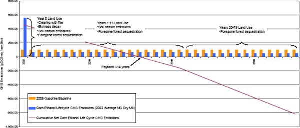
FIGURE G.5 Corn ethanol payback period.
SOURCE: Figure 2.6-14 from EPA (2010b).
Over long time periods, the different methods of accounting for ILUC-related GHG emission converge. ILUC emissions only occur as a result of increases in production capacity. At the end of the 30th year after the last increase in biofuel-production capacity, the accounting method that assumes a carbon debt in the first year that ILUC was incurred actually estimates larger GHG emission reductions from biofuels than the method that amortize the carbon debt over 30 years used by EPA and others. The 30-year amortization method implies that the initial ILUC-related GHG emissions are spread over the 30-year life of the biorefinery and continue to occur at 1/30 of the initial ILUC if the biorefinery continues to operate beyond 30 years. However, the 30-year amortization method underestimates cumulative GHG emissions over any time period when the biofuel expansion is ongoing. Therefore, the simplified first-year front-loading of ILUC-related GHG emissions is more in line with the importance of avoiding emissions sooner rather than later to minimize climatic risk (which is a scientific rationale for rapid GHG emissions reduction proposals analogous to those of this committee’s task statement).
Two different biofuel expansion cases are investigated in the modeling of this study. In the first case, biofuel-production capacity only expands to meet the RFS2 consumption mandates. This expansion is assumed to begin in 2011 and be complete for corn ethanol by 2013. Cellulosic-biofuel production to meet RFS2 is assumed to begin in 2015 and expand at an annual investment rate of about $10 billion per year (about 0.8 billion gallons per year of “drop-in” biofuels to meet the advanced and cellulosic biofuel requirements of 12.9 billion gge/year (20 billion gallons of ethanol equivalent per year by 2030) in RFS2.
In the second case, all future biofuels beyond the 15 billion gallons of corn-based ethanol are assumed to be produced from cellulosic biomass. Construction again begins in 2015, but investment is at the higher rate of about $10 billion per year. This investment rate would produce about 45 billion gge/year of drop-in biofuels by 2050, in addition to the 15 billion gallons per year of corn-grain ethanol that will be produced. That volume of cellulosic biofuels is required to meet the study objective of 80 percent reduction in use of petroleum-based fuels. The 45 billion gge/year of “drop-in” fuels will require 703 million dry tons of biomass per year.
The annual GHG emission profiles of these two expansion scenarios are given in Table G.6, which includes annual values for the calculated WTW GHG emissions relative to petroleum-based gasoline on a gallon of gasoline equivalent basis. WTW GHG emissions for petroleum-based gasoline are 98 kg CO2e/MMBtu or 11.38 kg CO2e/gge.
Although not analyzed here, another point to keep in mind is that all indirect land-use change attributable to biofuel system expansion is actually direct land-use change attributable to other uses in the location where it occurs. Land-use changes are driven in part by economic reasons; thus, it is reasonable
TABLE G.6 GHG Emissions for Biofuels Relative to Petroleum-Based Fuels
| Year | Only Meeting RFS2 | Maximum Biofuels | |||||||
| Corn-Grain Ethanol | “Drop-In” Cellulosic Biofuels | ||||||||
| Billion Gallons Per Year | Percent GHG Reduction Compared to Petroleum-Based Fuels | Billion gge/year | Percent GHG Reduction Compared to Petroleum-Based Fuels | Billion gge/year | GHG Reduction Compared to Petroleum-Based Fuels | ||||
| 2010 | 13 | 48.0 | |||||||
| 2011 | 14 | 118 | |||||||
| 2012 | 15 | 113 | |||||||
| 2013 | 15 | 48.0 | |||||||
| 2014 | 15 | 48.0 | |||||||
| 2015 | 15 | 48.0 | 0.8 | 507 | 1.9 | 507 | |||
| 2016 | 15 | 48.0 | 1.6 | 260 | 3.8 | 560 | |||
| 2017 | 15 | 48.0 | 2.3 | 177 | 5.8 | 177 | |||
| 2018 | 15 | 48.0 | 3.1 | 136 | 7.7 | 136 | |||
| 2019 | 15 | 48.0 | 3.9 | 111 | 9.6 | 111 | |||
| 2020 | 15 | 48.0 | 4.7 | 95.8 | 11.5 | 94.8 | |||
| 2021 | 15 | 48.0 | 5.5 | 83.1 | 13.4 | 83.1 | |||
| 2022 | 15 | 48.0 | 6.3 | 74.2 | 15.4 | 74.2 | |||
| 2023 | 15 | 48.0 | 7.0 | 67.4 | 17.3 | 67.4 | |||
| 2024 | 15 | 48.0 | 7.8 | 61.9 | 19.2 | 61.9 | |||
| 2025 | 15 | 48.0 | 8.6 | 57.4 | 21.1 | 57.4 | |||
| 2026 | 15 | 48.0 | 9.1 | 53.6 | 23.0 | 53.6 | |||
| 2027 | 15 | 48.0 | 10.2 | 50.4 | 25.0 | 50.4 | |||
| 2028 | 15 | 48.0 | 10.9 | 47.7 | 26.9 | 47.7 | |||
| 2029 | 15 | 48.0 | 11.7 | 45.4 | 28.8 | 45.4 | |||
| 2030 | 15 | 48.0 | 12.5 | 43.3 | 30.7 | 43.3 | |||
| 2031 | 15 | 48.0 | 12.5 | 12.4 | 32.6 | 41.5 | |||
| 2032 | 15 | 48.0 | 12.5 | 12.4 | 34.6 | 39.9 | |||
| 2033 | 15 | 48.0 | 12.5 | 12.4 | 36.5 | 38.4 | |||
| 2034 | 15 | 48.0 | 12.5 | 12.4 | 38.4 | 37.1 | |||
| 2035 | 15 | 48.0 | 12.5 | 12.4 | 40.3 | 35.9 | |||
| 2036 | 15 | 48.0 | 12.5 | 12.4 | 42.2 | 34.9 | |||
| 2037 | 15 | 48.0 | 12.5 | 12.4 | 44.2 | 33.9 | |||
| 2038 | 15 | 48.0 | 12.5 | 12.4 | 46.1 | 33.0 | |||
| 2039 | 15 | 48.0 | 12.5 | 12.4 | 48.0 | 32.2 | |||
| 2040 | 15 | 48.0 | 12.5 | 12.4 | 49.9 | 31.4 | |||
| 2041 | 15 | 48.0 | 12.5 | 12.4 | 51.8 | 30.7 | |||
| 2042 | 15 | 48.0 | 12.5 | 12.4 | 53.8 | 30.0 | |||
| 2043 | 15 | 48.0 | 12.5 | 12.4 | 55.7 | 29.4 | |||
| 2044 | 15 | 48.0 | 12.5 | 12.4 | 57.6 | 28.9 | |||
| 2045 | 15 | 48.0 | 12.5 | 12.4 | 59.5 | 28.3 | |||
| 2046 | 15 | 48.0 | 12.5 | 12.4 | 61.4 | 27.8 | |||
| 2047 | 15 | 48.0 | 12.5 | 12.4 | 63.4 | 27.4 | |||
| 2048 | 15 | 48.0 | 12.5 | 12.4 | 65.3 | 26.9 | |||
| 2049 | 15 | 48.0 | 12.5 | 12.4 | 67.2 | 26.5 | |||
| 2050 | 15 | 48.0 | 12.5 | 12.4 | 69.1 | 26.1 | |||
to expect that some of the wood in cleared forests might be harvested and used for other purposes rather than being immediately burned, as assumed in the ILUC calculations. This consideration would both reduce the first year GHG emissions and spread out the remaining emissions over a longer period of time.
This study also assumes that the ILUC attributable to cellulosic biofuels is that of switchgrass production. According to the U.S. Billion Ton Update, almost half of the biomass will be sourced from crop and forest residue (DOE, 2011). These biomass sources and some amount of farmed trees have little if any ILUC associated with their use, so the ILUC emissions estimated in this study could be high by a factor of two.
During the biomass conversion process, about 50 to 75 percent of the energy content of the biomass is burned during the production of the biofuel. Applying CCS technology to the biofuel production facilities would further reduce the GHG emissions attributable to biofuels. In addition, the LCA GHG emission calculations assume the current emissions profile from electricity generation and that all transportation fuels used to grow, harvest, and transport the biomass are produced from petroleum. As the electricity grid is decarbonized and the biofuel industry expands, the emissions from these sources will decrease as would the overall GHG emissions from biofuels.
G.6 INVESTMENT COSTS OF ELECTRICITY AS FUEL FOR ELECTRIC VEHICLES
There are four potential sources of investment costs for electricity as fuel to EVs:
• The charging stations to transfer energy from the electric power system to the vehicle.
• Additions or changes to the transmission and distribution system uniquely attributable to charging EVs.
• Additional generation capacity to charge EVs.
• Conversion of the existing power generation sources to a low GHG emitting set.
G.6.1 Charging Station Costs
The cost of installing a charging station consists of two parts: purchase of the physical charging station itself and installation of the charging station. The cost of the charging station is straightforward, but the cost of installation is highly variable. For the purpose of this study, an average of currently available charging station costs and the midrange estimate of expected installation costs was used. Cost of the equipment will drop in the future, but installation will not necessarily fall very much. We decreased the cost of the equipment by 67 percent in 2050, along a linear trend between 2010 and 2050 (Table G.7).
DC fast charging stations currently cost upwards of $20,000 for the equipment and are expensive to install because they have to connect to a higher voltage line than other charging equipment, and more site modification is expected. The DC charger price is expected to drop as additional large companies enter the market. Since the business case for electricity as fuel is not yet clear, the committee did not try to account for the commercial charging station investment, which is analogous to gasoline filling station costs. Furthermore, large numbers of public fast charging stations may not be required, since they primarily provide reassurance against range anxiety and are likely to primarily be used to connect cities along main travel lines and will not necessarily be widely available within cities. A study released by TEPCO (Botsford and Sczczepanek, 2009) showed that the addition of a second quick DC charger for their fleet in the Tokyo area increased the monthly mileage driven by a factor of 7. However, the number of vehicle charging events did not substantially increase, and the second charger did not receive significant use. Users drove the vehicles to lower battery levels knowing that there was a safety net. Based on these results, as well as user experiences in the United States (Turrentine et al., 2011) and Germany (Blanco, 2010), the committee considered that there will be fewer public chargers needed per vehicles after initial introduction. The committee’s specific assumptions are addressed below.
TABLE G.7 Charging Station Costs in 2011
| Charging Station | Equipment Range of Costs | Equipment Cost | Installation Range of Costs | Installation Cost | Total Cost Charging Station | ||||
| Level I— residential |
$450-$995 | $479 | $0-$500 | $200 | $679 | ||||
| Level II— residential |
$490-$1,200 | $892 | $300-$2,000 | $1,300 | $2,192 | ||||
| Level II— commercial |
$1,875-$4,500 | $2,477 | $1,000-$10,000 | $2,500 | $4,977 | ||||
| DC fast charge | $17,000-$44,000 | $34,200 | $7,000-$50,000 | $20,000 | $54,200 | ||||
To convert the charger costs to investment costs, the committee considered six different EVs: plug-in hybrid electric vehicle (PHEV)-10, PHEV-15, PHEV-20, PHEV-30, PHEV-40, and an all-electric BEV. (PHEV-XX is the designation of a PHEV with battery sized for XX miles of electric-only driving.) The committee also considered the two grid cases form the Annual Energy Outlook (AEO) 2011 report (EIA, 2011): the conventional grid and the low-GHG grid. Each vehicle is assumed to travel 13,000 miles per year with the fraction of electric miles taken from the NRC study Transitions to Alternative Transportation Technologies—Plug-in Hybrid Electric Vehicles (NRC, 2010): 20 percent electric miles for PHEV-10, 60 percent for PHEV-40, and 100 percent for the all EVs. For each vehicle, the committee assumed mix of charging stations typical for that class of PHEV. For a PHEV-10, one level 1 home charger and 0.25 of a level 1 charger at work was assumed for each vehicle (equaling $849 per vehicle in 2011). For a PHEV-40, one level 2 home charger and 0.4 of a commercial-grade level 2 charger was assumed for each vehicle (equaling $4,183 in 2011). For a battery electric vehicle (BEV), one level 2 home charger, 0.4 of a commercial charger, and 0.001 of a DC fast charger was assumed for each vehicle (equaling $4,725 in 2011). For PHEV-30, PHEV-40, and BEVs, the percentage of a public level II charging station decreases to 0.3 in 2020, 0.2 in 2030, and 0.1 in 2040.
For each vehicle, the committee amortized the cost of this mix of chargers over 15 years to get an annual cost and converted it to a cost per kilowatt-hour (based on the annual energy use of each vehicle. The total cost of electricity into the vehicle is the sum of the charger cost per kilowatt-hour added to the cost of the electricity drawn from the grid, using residential rates in the appropriate year, and tabulated separately for both the reference and low GHG grid. Investment costs are also calculated in units of $/kWh/day and $/gge/day for comparison to other fuel systems. The results are shown in Tables G.8 and G.9 for the reference grid and the low-GHG grid, respectively.
G.6.2 Investment Costs for Transmission and Distribution System Changes Uniquely Required to Accommodate EV Charging
The primary impact will be on the local distribution system; changes to the high voltage transmission system will be included in the cost of new power generation systems and are discussed later in this appendix. As discussed briefly in chapter 3, studies by EPRI (EPRI, 2004, 2005), discussions by the committee with PG&E (Takemasa, 2011), and previous discussions with SCE earlier (Cromie and Graham, 2009) indicate these costs are manageable and within the normal costs of doing business. The continuing replacement, upgrade, and expansion costs are reflected in the cost of electricity provided to customers.
TABLE G.8 Reference Grid
| 2010 | 2020 | 2035 | 2050 | ||||||
| PHEV-10 | |||||||||
| AEO base elec cost, $/kWh | 0.096 | 0.088 | 0.092 | 0.094 | |||||
| Charger cost, $/car | 849 | 748 | 598 | 448 | |||||
| Charger cost, $/kWh | 0.066 | 0.058 | 0.047 | 0.035 | |||||
| Into LDV elec cost, $/kWh | 0.162 | 0.146 | 0.139 | 0.129 | |||||
| AEO GHG, MMTCO2 | 2499 | 2418 | 2753 | 3042 | |||||
| WTT GHG kgCO2/kWh | 0.631 | 0.582 | 0.594 | 0.592 | |||||
| WTT GHG, kg CO2/gge | 21.06 | 19.42 | 19.85 | 19.78 | |||||
| Investment, $/kWh/day | 362 | 319 | 255 | 191 | |||||
| Investment, $/gge/day | 12317 | 10862 | 8679 | 6495 | |||||
| PHEV-15 | |||||||||
| AEO base elec cost, $/kWh | 0.096 | 0.088 | 0.092 | 0.094 | |||||
| Charger cost, $/car | 849 | 748 | 598 | 448 | |||||
| Charger cost, $/kWh | 0.048 | 0.042 | 0.034 | 0.025 | |||||
| Into LDV elec cost, $/kWh | 0.144 | 0.130 | 0.126 | 0.119 | |||||
| AEO GHG, MMTCO2 | 2499 | 2418 | 2753 | 3042 | |||||
| WTT GHG kgCO2/kWh | 0.631 | 0.582 | 0.594 | 0.592 | |||||
| WTT GHG, kg CO2/gge | 21.06 | 19.42 | 19.85 | 19.78 | |||||
| Investment, $/kWh/day | 260 | 230 | 183 | 137 | |||||
| Investment, $/gge/day | 8853 | 7807 | 6238 | 4669 | |||||
| PHEV-20 | |||||||||
| AEO base elec cost, $/kWh | 0.096 | 0.088 | 0.092 | 0.094 | |||||
| Charger cost, $/car | 849 | 748 | 598 | 448 | |||||
| Charger cost, $/kWh | 0.038 | 0.034 | 0.027 | 0.020 | |||||
| Into LDV elec cost, $/kWh | 0.134 | 0.122 | 0.119 | 0.114 | |||||
| AEO GHG, MMTCO2 | 2499 | 2418 | 2753 | 3042 | |||||
| WTT GHG kgCO2/kWh | 0.631 | 0.582 | 0.594 | 0.592 | |||||
| WTT GHG, kg CO2/gge | 21.06 | 19.42 | 19.85 | 19.78 | |||||
| Investment, $/kWh/day | 208 | 184 | 147 | 110 | |||||
| Investment, $/gge/day | 7082 | 6246 | 4990 | 3735 | |||||
| PHEV-30 | |||||||||
| AEO base elec cost, $/kWh | 0.096 | 0.088 | 0.092 | 0.094 | |||||
| Charger cost, $/car | 4183 | 3411 | 2606 | 1926 | |||||
| Charger cost, $/kWh | 0.139 | 0.113 | 0.087 | 0.064 | |||||
| Into LDV elec cost, $/kWh | 0.235 | 0.201 | 0.179 | 0.158 | |||||
| AEO GHG, MMTCO2 | 2499 | 2418 | 2753 | 3042 | |||||
| WTT GHG kgCO2/kWh | 0.631 | 0.582 | 0.594 | 0.592 | |||||
| WTT GHG, kg CO2/gge | 21.06 | 19.42 | 19.85 | 19.78 | |||||
| Investment, $/kWh/day | 760 | 620 | 474 | 350 | |||||
| Investment, $/gge/day | 25854 | 21085 | 16111 | 11906 | |||||
| PHEV-40 | |||||||||
| AEO base elec cost, $/kWh | 0.096 | 0.088 | 0.092 | 0.094 | |||||
| Charger cost, $/car | 4183 | 3411 | 2606 | 1926 | |||||
| Charger cost, $/kWh | 0.123 | 0.100 | 0.077 | 0.057 | |||||
| Into the LDV elec cost, $/kWh | 0.219 | 0.188 | 0.169 | 0.151 | |||||
| AEO GHG, MMTCO2 | 2499 | 2418 | 2753 | 3042 | |||||
| WTT GHG kg CO2/kWh | 0.631 | 0.582 | 0.594 | 0.592 | |||||
| WTT GHG, kg CO2/gge | 21.06 | 19.42 | 19.85 | 19.78 | |||||
| Investment, $/kWh/day | 673 | 549 | 419 | 310 | |||||
| Investment, $/gge/day | 22888 | 18666 | 14262 | 10539 | |||||
| Battery Electric | |||||||||
| AEO base elec cost, $/kWh | 0.096 | 0.088 | 0.092 | 0.094 | |||||
| Charger cost, $/car | 4237 | 3460 | 2646 | 1957 | |||||
| Charger cost, $/kWh | 0.076 | 0.062 | 0.047 | 0.035 | |||||
| Into the LDV elec cost, $/kWh | 0.172 | 0.150 | 0.139 | 0.129 | |||||
| AEO GHG, MMTCO2 | 2499 | 2418 | 2753 | 3042 | |||||
| WTT GHG kg CO2/kWh | 0.631 | 0.582 | 0.594 | 0.592 | |||||
| WTT GHG, kg CO2/gge | 21.06 | 19.42 | 19.85 | 19.78 | |||||
| Investment, $/kWh/day | 416 | 340 | 260 | 192 | |||||
| Investment, $/gge/day | 14142 | 11548 | 8833 | 6533 | |||||
TABLE G.9 Low GHG Grid Case
| 2010 | 2020 | 2035 | 2050 | ||||||
| PHEV-10 | |||||||||
| AEO base elec cost, $/kWh | 0.096 | 0.112 | 0.126 | 0.148 | |||||
| Charger cost, $/car | 849 | 748 | 598 | 448 | |||||
| Charger cost, $/kWh | 0.066 | 0.058 | 0.047 | 0.035 | |||||
| Into LDV elec cost, $/kWh | 0.162 | 0.170 | 0.173 | 0.183 | |||||
| AEO GHG, MMTCO2 | 2516 | 1771 | 1270 | 648 | |||||
| WTT GHG kg CO2/kWh | 0.635 | 0.463 | 0.319 | 0.155 | |||||
| WTT GHG, kg CO2/gge | 21.21 | 15.48 | 10.67 | 5.17 | |||||
| Investment, $/kWh/day | 362 | 319 | 255 | 191 | |||||
| Investment, $/gge/day | 12317 | 10862 | 8679 | 6495 | |||||
| PHEV-15 | |||||||||
| AEO base elec cost, $/kWh | 0.096 | 0.112 | 0.126 | 0.148 | |||||
| Charger cost, $/car | 849 | 748 | 598 | 448 | |||||
| Charger cost, $/kWh | 0.048 | 0.042 | 0.034 | 0.025 | |||||
| Into LDV elec cost, $/kWh | 0.144 | 0.130 | 0.126 | 0.119 | |||||
| AEO GHG, MMTCO2 | 2516 | 1771 | 1270 | 648 | |||||
| WTT GHG kg CO2/kWh | 0.635 | 0.463 | 0.319 | 0.155 | |||||
| WTT GHG, kg CO2/gge | 21.21 | 15.48 | 10.67 | 5.17 | |||||
| Investment, $/kWh/day | 260 | 230 | 183 | 137 | |||||
| Investment, $/gge/day | 8853 | 7807 | 6238 | 4669 | |||||
| PHEV-20 | |||||||||
| AEO base elec cost, $/kWh | 0.096 | 0.112 | 0.126 | 0.148 | |||||
| Charger cost, $/car | 849 | 748 | 598 | 448 | |||||
| Charger cost, $/kWh | 0.038 | 0.034 | 0.027 | 0.020 | |||||
| Into LDV elec cost, $/kWh | 0.134 | 0.122 | 0.119 | 0.114 | |||||
| AEO GHG, MMTCO2 | 2516 | 1771 | 1270 | 648 | |||||
| WTT GHG kg CO2/kWh | 0.635 | 0.463 | 0.319 | 0.155 | |||||
| WTT GHG, kg CO2/gge | 21.21 | 15.48 | 10.67 | 5.17 | |||||
| Investment, $/kWh/day | 208 | 184 | 147 | 110 | |||||
| Investment, $/gge/day | 7082 | 6246 | 4990 | 3735 | |||||
| PHEV-30 | |||||||||
| AEO base elec cost, $/kWh | 0.096 | 0.112 | 0.126 | 0.148 | |||||
| Charger cost, $/car | 4183 | 3411 | 2606 | 1926 | |||||
| Charger cost, $/kWh | 0.139 | 0.113 | 0.087 | 0.064 | |||||
| Into LDV elec cost, $/kWh | 0.235 | 0.201 | 0.179 | 0.158 | |||||
| AEO GHG, MMTCO2 | 2516 | 1771 | 1270 | 648 | |||||
| WTT GHG kg CO2/kWh | 0.635 | 0.463 | 0.319 | 0.155 | |||||
| WTT GHG, kg CO2/gge | 21.21 | 15.48 | 10.67 | 5.17 | |||||
| Investment, $/kWh/day | 760 | 620 | 474 | 350 | |||||
| Investment, $/gge/day | 25854 | 21085 | 16111 | 11906 | |||||
| PHEV-40 | |||||||||
| AEO base elec cost, $/kWh | 0.096 | 0.112 | 0.126 | 0.148 | |||||
| Charger cost, $/car | 4183 | 1967 | 1266 | 690 | |||||
| Charger cost, $/kWh | 0.123 | 0.058 | 0.037 | 0.020 | |||||
| Into the LDV elec cost, $/kWh | 0.219 | 0.170 | 0.163 | 0.168 | |||||
| AEO GHG, MMTCO2 | 2516 | 1771 | 1270 | 648 | |||||
| WTT GHG kg CO2/kWh | 0.635 | 0.463 | 0.319 | 0.155 | |||||
| WTT GHG, kg CO2/gge | 21.21 | 15.48 | 10.67 | 5.17 | |||||
| Investment, $/kWh/day | 673 | 549 | 419 | 310 | |||||
| Investment, $/gge/day | 22888 | 18666 | 14262 | 10539 | |||||
| Battery Electric | |||||||||
| AEO base elec cost, $/kWh | 0.096 | 0.112 | 0.126 | 0.148 | |||||
| Charger cost, $/car | 4237 | 3460 | 2646 | 1957 | |||||
| Charger cost, $/kWh | 0.076 | 0.062 | 0.047 | 0.035 | |||||
| Into the LDV elec cost, $/kWh | 0.172 | 0.174 | 0.173 | 0.183 | |||||
| AEO GHG, MMTCO2 | 2516 | 1771 | 1270 | 648 | |||||
| WTT GHG kg CO2/kWh | 0.635 | 0.463 | 0.319 | 0.155 | |||||
| WTT GHG, kg CO2/gge | 21.21 | 15.48 | 10.67 | 5.17 | |||||
| Investment, $/kWh/day | 416 | 340 | 260 | 192 | |||||
| Investment, $/gge/day | 14142 | 11548 | 8833 | 6533 | |||||
Some utilities have noted the current on-board chargers in EVs limit power flow to about 3.3 kW. If, in the future, larger on-board chargers are used to reduce charging time (e.g., 8 to 15 kW), then the resultant energy flow would challenge the capacity of many residential power systems, even for a single charging installation, and for commercial building power systems where multiple charging stations were installed. This may require more extensive upgrading of the local distribution system, as well as building wiring changes. As a result, the utilities may charge increased fees beyond those covered by the cost of electricity. However, such costs are uncertain and difficult to quantify. The committee did not add additional investment costs in this category.
G.6.3 Additional Generation Capacity to Charge Electric Vehicles
The committee estimated the power on the grid required to fuel 100 million EVs in 2050 is about 286 billion kWh. If much of this charging is done off-peak, then a lesser amount of power is needed, and, as noted in chapter 3, depending on the region of the country, there may be considerable off-peak or reserve capacity. However, it is conservative to estimate the additional power and its cost on the basis that all of what is needed is new capacity. Furthermore, in the case of the AEO low-GHG grid case, the power growth from 2020 to 2050 is very low, probably inhibited by the high cost of electricity, which drives more efficient use of the installed generation sources. Hence, there is likely lower margin in the low-GHG grid and there may already be considerable off-peak use. Furthermore, the low-GHG grid does not assume a large use of electricity for transportation purposes. So the additional power generation capacity is estimated as being that which is added to the low-GHG grid case to charge 100 million EVs in 2050.
The average capacity factor for the new plants is assumed to be 0.4, since they will likely be a mix of gas plants with high-capacity factor and renewables with lower-capacity factor. For an additional generation capacity of 286,000,000 megawatt-hours, this translates to 90,000 MW of installed capacity. Assuming an average cost of $4,000,000 per megawatt, a total investment of $360 billion will be required. Some additional investment will be required to expand the high-voltage transmission system to carry this power to the load centers where it is further distributed by the lower-voltage distribution system. The total cost will be approximately $400 billion or more.
This capital cost is reflected in the cost of electricity to the customer and is not a separate cost. However, this large amount of capital will be needed to finance building the needed infrastructure as the generation expands as required to fuel the EVs. The utilities will recoup this cost plus a return on investment over a long period of time from the ratepayers.
G.6.4 Conversion of Existing Power Generation Sources to Low-GHG Emissions
Beyond the investment needed to provide the incremental power for EVs, there is an additional cost required to convert the existing grid to produce much lower emissions of GHGs, especially CO2. This is because the grid does not preferentially transmit power from particular plants to specific loads. Even if sufficient capacity is added to the grid to produce the power for the EVs, and it is all low-GHG emitting, the full benefit of using EVs to reduce GHG emissions will not be achieved unless the whole grid has much lower GHG emissions on the average.
Table G.10 shows the generation mix for both the reference case and the low-GHG case in 2035. These data show there is a shift in the generation mix to reduce GHG emissions. The dominant changes are that coal, natural gas, and oil-fired sources of steam to produce electricity drop by about 130 gigawatt (GW) and about 180 GW of nuclear, renewable, and combined cycle natural gas generation are added. The low-GHG grid grows by about 35 GW from 2010 value (See Table 3.8 in Chapter 3 of the main report) so about 145 GW of new power is added for GHG reduction and as existing assets are retired. Assuming an average cost of $4 billion per GW for new capacity, the cost of the conversion is $500 billion to $600 billion through 2035.
TABLE G.10 2035 Net Summer Capacity and Electricity Production
| Source | Reference Case Net Summer Capacity (GW) | Reference Electricity Production (Thousands GWhr) | Low GHG Case Net Summer Capacity (GW) | Low-GHG Electricity Production (Thousands GWhr) | |||||
| Coal | 317.9 | 2137.6 | 191.2 | 807.1 | |||||
| Oil and natural gas steam | 88.7 | 124.7 | 84.4 | 123.8 | |||||
| Natural gas combined cycle | 315.3 | 892.1 | 263.3 | 1203 | |||||
| Diesel/conventional combustion turbine | 181.6 | 52.3 | 149.2 | 769 | |||||
| Nuclear | 110.5 | 874.4 | 133.6 | 1052 | |||||
| Pumped storage | 21.8 | -0.1 | 21.8 | -0.1 | |||||
| Renewables | 148.5 | 547.6 | 204 | 737 | |||||
| Distributed generation | 3.1 | 4.6 | 0.5 | 0.6 | |||||
| Total | 1131.7 | 4633.2 | 1048.8 | 3976 | |||||
Additional low-GHG generation sources must be added to the grid between 2035 and 2050, since the GHG emissions per kilowatt-hour of generation in 2050 needs to be about half that of 2035 to meet the 80 percent reduction goal in annual emissions. (See Table 3.8 in Chapter 3 of the main report.) Between 2035 and 2050 the low-GHG grid installed capacity is expected to grow by about 5 percent or 50-60 GW. Even if all this new capacity is low-GHG emissions, it is not sufficient to reduce the GHG emission by the desired amount. So more existing assets need to be retired or replaced and additional low-GHG emitting sources added. An amount will be needed that is comparable to the power sources added between 2010 and 2035. This suggests the total new capital needed to convert the U.S. electric power system to achieve an 80 percent reduction in annual GHG emissions by 2050 is of the order of $1 trillion.
G.7 THE USE OF NATURAL GAS TO POWER LIGHT-DUTY VEHICLES
Natural gas could contribute a significant portion of liquid fuels for light-duty vehicles (LDVs) in the United States by 2050 because it is a domestic, low-cost, and plentiful fuel with GHG emissions lower than petroleum-based fuels. However, the optimal mix of technologies for producing natural gas-based fuels is unclear. Issues include the cost of 1 gge in comparison with petroleum-based fuels, the need for any new fuel manufacturing and distribution infrastructure, the minimum economic increment of infrastructure investment, the availability and cost of vehicle technologies suitable for the particular fuel, and the life-cycle GHG emissions of the various natural gas-based fuel and vehicle technologies.
G.7.1 Advantages and Challenges of Each Pathway
G.7.1.1 Compressed Natural Gas for Direct Fueling
Advantages
• One gallon of gasoline equivalent of compressed natural gas (CNG) is cheaper than 1 gallon of petroleum-based gasoline.
• The technology is proven and available.
• Fuel distribution pipelines are in place and can supply initial requirements.
• Tailpipe emissions are much lower compared to petroleum-based gasoline.
Challenges
• CNG fuel stations are few and expensive to build.
• Dedicated CNG vehicles need to be designed (engines, trunk space, range).
• At low CNG LDV volumes and corresponding high CNG vehicle prices, and at the price differential between natural gas and gasoline observed in 2012, CNG vehicles are not economical.
G.7.1.2 Natural Gas for Electricity (PHEV and BEV)
Advantages
• Fuel cost per gallon of gasoline equivalent is low.
• There are no tailpipe emissions.
• Home charging stations can be sold at reasonable cost.
• Incremental capital investment into electricity infrastructure is minimal.
Challenges
• The batteries are expensive.
• Reasonably sized batteries provide short BEV range.
• PHEVs and BEVs are expensive.
• BEV batteries have long charging times.
G.7.1 3 Natural Gas to Liquid (Hydrocarbon) Fuels (Fischer-Tropsch and via Methanol-to-Gasoline)
Advantages
• Drop-in hydrocarbon fuels are produced.
• Distribution, dispensing, and vehicle infrastructure and technology are in place.
• Chemical process technology is proven.
Challenges
• Large investments in minimum incremental fuels plants create investment risk.
• Tailpipe emissions need to be controlled.
• GHG emissions are high relative to other alternative fuels.
G.7.1.4 Natural Gas to Methanol (“The Methanol Economy”)
Advantages
• Methanol is an excellent fuel in neat form or in low and high mixtures with gasoline.
• Minimal to no changes to engines required.
• Infrastructure for filling stations already exists.
• Life-cycle GHG emissions of natural gas to methanol is lower than those of petroleum-based gasoline.
Challenges
• Methanol has half the volumetric energy content of gasoline. The size of fuel tanks may need to be increased, depending on the mixing ratio of methanol and gasoline.
• Transdermal and inhalation toxicity debate needs to be settled.
• Movement and residence time in ground water debate needs to be settled.
• Methanol is corrosive to aluminum and certain plastic pipes and gaskets.
G.7.1.5 Natural Gas to Hydrogen
Advantages
• There are no tailpipe emissions.
• Hydrogen can be made from locally distributed natural gas without the need for a hydrogen pipeline infrastructure.
• Its initial introduction can rely on existing hydrogen supply chain.
Challenges
• Methane-to-hydrogen is more expensive than gasoline on a unit gallon of gasoline equivalent basis.
• Hydrogen pipeline infrastructure is necessary for large-scale use.
• Investment in hydrogen filling stations will be necessary.
• Vehicular hydrogen storage tanks are expensive.
G.7.2 Comparing the Efficiency of Different Options for Using Natural Gas as a LDV Fuel
Comparing these options can be difficult. However, a comparison based solely on use of the efficiency of energy in the gas removes many of the uncertainties. Such a comparison was made based on the vehicle fuel-utilization efficiencies of Chapter 2 and the fuel-conversion efficiencies of Chapter 3. The candidate vehicle propulsion systems include conventional internal combustion engines (ICEs) and advanced technologies such as EVs and FCEVs. Electric vehicles include conventional hybrid vehicles (HEVs), PHEVs, and BEVs. These vehicles differ in the size of the battery and electric motor compared with the ICE. An FCEVs also uses a battery and an electric motor, but replaces the ICE with a hydrogen fuel cell.
Table G.11 shows annual total natural gas usage if the entire LDV fleet was powered with conventional ICEs using natural gas as fuel from various pathways. The most efficient use of natural gas is direct use as CNG.
Table G.12 compares the annual natural gas usage if the entire LDV fleet were powered by electric or fuel-cell vehicles using natural gas as fuel via different pathways. These alternative vehicle technologies all require technology advances to be cost competitive with conventional ICEs.
At the beginning of the time period, efficiency favors the BEVs, but BEV technology is not technologically or economically competitive in the 2010-2030 time frame. (See Chapter 5.) By 2050, the efficiency of the propulsion technologies of HEVs, PHEVs, EVs, and FCEVs differ by less than 10 percent, which is within the uncertainty of the estimate. There is no clear winner based only on overall energy efficiency.
TABLE G.11 Total Natural Gas Usage If the Entire Light-Duty Vehicle Fleet Were to Be Powered by Conventional ICEs Using Natural Gas
| Year | Total Natural Gas Usage, trillion cubic feet per year | ||||||||
| Total Vehicle Miles Traveled (trillion) | Compressed Natural Gas | Drop-In Hydrocarbon Fuels | Methanol | ||||||
| 2010 | 2.784 | 15.6 | 23.8 | 22.9 | |||||
| 2030 | 3.727 | 10.1 | 15.5 | 14.9 | |||||
| 2050 | 5.048 | 10.0 | 15.4 | 14.8 | |||||
TABLE G.12 Comparison of Natural Gas Usage If the Entire Light-Duty Vehicle Fleet Were to Be Powered by Electric or Fuel-Cell Vehicles Using Natural Gas Via Different Pathways
| Year | Total Natural Gas Usage, trillion cubic feet per year | ||||||||
| Total Vehicle Miles Traveled (trillion) | HEV Powered by CNG and Gasoline | Full BEV | FCEV | ||||||
| 2010 | 2.784 | 15.1 | 7.6 | 11.7 | |||||
| 2030 | 3.727 | 8.4 | 7.5 | 7.3 | |||||
| 2050 | 5.048 | 7.9 | 7.8 | 7.2 | |||||
G.8 METHANOL AS A FUEL OR FUEL ADMIXTURE
Methanol as an automobile fuel has been used for years. Beyond decades of use in motor racing, methanol was used for 25 years by the public to drive about 200 million miles in California between 1980 and 2005. According to DOE’s Energy Information Administration (EIA) (Joyce, 2012), methanol’s decline might have been prompted in part by the occasional dramatic increases in natural gas prices, from which methanol is manufactured. Methanol is one of the alternative fuels being pursued in China.
Methanol is less volatile than gasoline, and, therefore, it is considered to have better fire safety. It can be mixed with gasoline by different proportions—it can be used as neat methanol, a mixture of 85 percent gasoline and 15 percent methanol (which may require no engine adjustment of a gasoline-powered ICE), or a mixture of 85 percent methanol and 15 percent gasoline. Methanol has a high octane number (114), and liquid methanol has a higher energy content (per volume) than liquid hydrogen. Methanol is made primarily from natural gas, but it can also be made from coal (both via syngas, CO, and H2). With the abundant resources of natural gas and coal in the United States, methanol supply would be ensured. Methanol has about half of gasoline’s volumetric energy content (2.01 gallon of methanol = 1 gge). Methanol prices in 2012 were less than $0.50/gallon. Therefore, methanol would be an economically attractive alternative fuel or fuel additive. A “methanol economy” that includes methanol manufacture via the hydrogenation of sequestered CO2 has been proposed (Olah et al., 2006).
So, why is the use of methanol as a fuel declining with an unsure prospect in the United States? Methanol has some of the same drawbacks as ethanol, and these can be managed the same way. Methanol is hygroscopic. It is a solvent for some plastics and corrodes aluminum, and, therefore, it is incompatible with some automotive tubing materials. The major concerns with methanol as an automobile fuel seem to be focused on environmental and health issues (see Malcolm Pirnie, 1999, for examples). Methanol is toxic, but the OSHA 40-hour exposure level of methanol (1,260 mg/m2) is comparable to those of gasoline (900 mg/m2) and ethanol (1,900 mg/m2). There may be insufficient data about the health effects of inhaled and skin-penetrated methanol (while ingested methanol is well understood). There are conflicting data about the potential effects of spilled or leaked methanol on ground water (for example, its
rate of penetration and half-life in the soil; Smith et al., 2003). Given the negative experiences with methyl tertiary butyl ether, concern has been raised about repeating those experiences with methanol.
With the recent emergence of plentiful and potentially cheap natural gas and, therefore, the potential for plentiful and cheap methanol, methanol will likely remain under consideration as an alternative fuel, probably prompting further studies of its environmental characteristics and health effects.
G.9 INFRASTRUCTURE AND IMPLEMENTATION FOR COMPRESSED NATURAL GAS AS AN AUTOMOBILE FUEL
G.9.1 Capital Costs of the Natural Gas Pipeline Infrastructure
The EIA forecasts show significant increases in future natural gas usage, albeit not for automotive use. From 2008 to 2035, the United States and Canada natural gas pipeline infrastructure has been projected to increase from a capacity of 26.8 trillion of standard cubic feet per year to 31.8 to 36 trillion of standard cubic feet per year (EIA, 2011). The corresponding investment will be $133 billion to $210 billion, divided between transmission (80 to 83 percent), storage (1 percent), gathering (7 to 8 percent), processing (7 to 8 percent), and liquefied natural gas (1 percent). These projections are for the combined U.S. and Canadian infrastructure. About 12 percent of the natural gas consumed in the United States in 2009 was imported from Canada, and thus Canada has part of the natural gas pipeline infrastructure required to supply the U.S. consumption. In a report addressing the same issues, ICF International (2009) concluded that between 2009 and 2030, the United States and Canada will need 28,900 to 61,000 miles of additional natural gas pipeline and 371 to 598 billion cubic feet (bcf) additional storage capacity to satisfy projected natural gas market requirements. None of these projections appear to account for any significant increase in natural gas use for automobile transportation. Because of the low projected volumes of natural gas used in transportation during this time period, the growth of the CNG fleet is unlikely to be limited by pipeline infrastructure for natural gas, as already mentioned before.
G.9.2 CNG Filling Station Capital Costs
As of February 2010, the United States had 247 million registered road vehicles (136 million cars, 110 million trucks, and 1 million buses). These were served by 159,006 “retail gasoline outlets” (gas stations) at a ratio of 1,553 vehicles/gas station. As of 2010, the global ratio of natural gas vehicles to filling stations was 685 vehicles per station (Pike Research, 2011). At the same time, the United States had a total of 1,327 natural gas filling stations (private and public-access combined). Only 60 of the stations were for LNG, and the majority was for CNG. The economic difficulties in building a dispensing infrastructure for natural gas are illustrated by the fact that these 1,327 natural gas filling stations in the United States serve only a total of 112,000 vehicles in the country, for a ratio of 84 natural gas vehicles per filling station. This is most likely an uneconomically small ratio for an independent, for-profit, public-access natural gas filling station. For 2016, Pike Research (2011) forecasted that the number natural gas vehicles will increase at a rate of 8 percent per year, while the number of natural gas filling stations will increase only at 5 percent per year.
There are four types of natural gas filling station designs: time filling (mostly for home use, 8 hours), cascade fast-fill (public access, with natural gas storage), central fast-fill (buffered, for large vehicles), and combined CNG/LNG stations. Natural gas filling station costs have been discussed by the DOE’s Idaho National Laboratory (INL, 2005). For storage and dispensing equipment only (no buildings and land), LNG stations were estimated to cost $0.35 million to $1 million, in comparison for gasoline-station equipment at $0.15 million. It appears that CNG filling stations will be fairly modular so that their cost will likely scale somewhat linearly with dispensing capacity.
An investment opportunity for CNG filling stations was published recently on the Internet (International CNG, 2012). It suggested that a $1.75 million investment is needed into a CNG station located in the District of Columbia, Maryland, or Virginia. A station would serve 1,000 cars per week, 10 gge/fill/car/week, with $0.50 margin over the cost of natural gas for a 15 percent return on investment.
The natural gas filling station infrastructure costs can be estimated based on the above investment offer by assuming one filling station per 1,000 CNG vehicles and a cost of $1.3 million per filling station (land, buildings, and equipment). On that basis, for example, for 5 million CNG vehicles, the filling station infrastructure would cost about $6.5 billion. CNG compressing and dispensing equipment is being sold by the clean-energy company IMW Industries at the writing of this report.
For municipal CNG vehicle fleets, the National Renewable Energy Laboratory report (Johnson, 2010) analyzes the business case for filling stations. A model has been developed that allows an investor to compute capital requirements and returns as a function of a number of equipment and operating variables.
The price of home-dispensed CNG can be significantly lower than filling station-dispensed CNG. As a result, CNG vehicle owners have been interested in home refueling. Honda Civic GX owners in California were able to purchase a home-fill station for overnight refueling for about $4,500 and have it installed at an additional fee. As of this writing, Honda is not recommending the home refueling of their CNG vehicles, due in part to concerns about the humidity content of home natural gas.
G.10 REFERENCES
Blanco, S. 2010. In Depth: BWM Megacity Vehicle and Project I. Available at http://green.autoblog.com/2010/07/02/in-depth-bmw-megacity-vehicle-and-project-i/. Accessed on January 7, 2011.
Botsford, C., and A. Sczczepanek. 2009. Fast charging vs.slow charging: Pros and cons for the new age of electric vehicles. In EVS24 International Battery, Hybrid and Fuel Cell Electric Vehicle Symposium. Stravanger, Norway.
Cromie, R., and R. Graham. 2009. Transition to Electricity as the Fuel of Choice. Presentation to the NRC Committee on Assessment of Resource Needs for Fuel Cell and Hydrogen Technologies on May 18.
Davis, R., A. Aden, and P.T. Pienkos. 2011. Techno-economic analysis of autotrophic microalgae for fuel production. Applied Energy 88(10):3524-3531.
DOE (U.S. Department of Energy). 2010a. Algenol Integrated Biorefinery for Producing Ethanol from Hybrid Algae. DOE/EA-1786. Washington, D.C.: U.S. Department of Energy.
———. 2010b. National Algal Biofuels Technology Roadmap. Washington, D.C.: U.S. Department of Energy, Office of Energy Efficiency and Renewable Energy.
———. 2011. U.S. Billion-Ton Update. Washington, D.C.: U.S. Department of Energy. Available at http://www1.eere.energy.gov/biomass/pdfs/billion_ton_update.pdf.
EIA (Energy Information Administration). 2011. Annual Energy Outlook 2011 With Projections to 2035. Washington, DC: U.S. Department of Energy.
EPA (U.S. Environmental Protection Agency). 2010a. Regulation of fuels and fuel additives: Changes to renewable fuel standard program; final rule. Federal Register 75(58):14669-15320.
———. 2010b. Renewable Fuel Standard Program (RFS2) Regulatory Impact Analysis. US EPA 420-R-10-006. Washington, D.C.: U.S. Environmental Protection Agency.
EPRI (Electric Power Research Institute). 2004. Advanced Batteries for Electric-Drive Vehicles. A Technology and Cost-Effectiveness Assessment for Battery Electric Vehicles, Power Assist Hybrid Electric Vehicles, and Plug-In Hybrid Electric Vehicles. Palo Alto, Calif.: Electric Power Research Institute.
———. 2005. Plug-in Hybrid Electric Vehicles: Changing the Energy Landscape. Palo Alto, Calif.: Electric Power Research Institute.
Hertel, T.W., A.A. Golub, A.D. Jones, M. O’Hare, R.J. Plevin, and D.M. Kammen. 2010. Effects of US maize ethanol on global land use and greenhouse gas emissions: estimating market-mediated responses. BioScience 60(3):223-231.
Howard, J.L. 2007. U.S. Timber Production, Trade, Consumption, and Price Statistics 1965 to 2005. Madison, Wis.: U.S. Department of Agriculture, Forest Service.
ICF International. 2009. Natural Gas Pipeline and Storage Infrastructure Projections Through 2030. Washington, D.C.: ICF International.
INL, (Idaho National Laboratories). 2005. Natural gas technologies. Low-cost refueling station. Available at http://www.inl.gov/lng/projects/refuelingstation.shtml. Accessed on January 16, 2011.
International CNG, Inc. 2012. International CNG, Inc. Refueling America and American Innovation Investment Opportunity. Available at http://www.internationalcng.com/cng-1_com/bank/pageimages/cng_investment_brochure.pdf. Accessed on March 23, 2012.
Jager, H., L.M. Baskaran, C.C. Brandt, E.B. Davis, C.A. Gunderson, and S.D. Wullschleger. 2010. Empirical geographic modeling of switchgrass yields in the United States. Global Change Biology Bioenergy 2 (5):248-257.
Johnson, C. 2010. Business Case for Compressed Natural Gas in Municipal Fleets. Golden, Colo.: National Renewable Energy Laboratory.
Joyce, M. 2012. Developments in U.S. alternative fuel markets. Available at http://www.eia.gov/cneaf/alternate/issues_trends/altfuelmarkets.html. Accessed on Janaury 19, 2012.
Malcolm Pirnie. 1999. Evaluation of the Fate and Transport of Methanol in the Environment. Oakland, Calif.: Malcolm Pirnie.
Marshall, E., M. Caswell, S. Malcolm, M. Motamed, J. Hrubovcak, C. Jones, and C. Nickerson. 2011. Measuring the Indirect Land-Use Change Associated With Increased Biofuel Feedstock Production. A Review of Modeling Efforts. Report to Congress. Washington, D.C.: U.S. Department of Agriculture, Economic Research Service.
NAS-NAE-NRC, (National Academy of Sciences, National Academy of Engineering, National Research Council). 2009. Liquid Transportation Fuels from Coal and Biomass: Technological Status, Costs, and Environmental Impacts. Washington, D.C.: The National Academies Press.
NRC (National Research Council). 2010. Transitions to Alternative Transportation Technologies—Plug- in Hybrid Electric Vehicles. Washington, D.C.: The National Academies Press.
———. 2011. Renewable Fuel Standard: Potential Economic and Environmental Effects of U.S. Biofuel Policy. Washington, D.C.: The National Academies Press.
Olah, G.A., A. Goeppert, and G.K.S. Prakash. 2006. Beyond Oil and Gas: The Methanol Economy. Weinheim, Germany: Wiley.
Perlack, R.D., L.L. Wright, A.F. Turhollow, R.L. Graham, B.J. Stokes, and D.C. Erbach. 2005. Biomass as Feedstock for a Bioenergy and Bioproducts Industry: The Technical Feasibility of a Billion-Ton Annual Supply. Oak Ridge, Tenn.: U.S. Department of Energy, U.S. Department of Agriculture.
Pike Research. 2011. Natural Gas Vehicles. Market Analysis and Global Forecasts for CNG and LNG Cars, Trucks, and Buses. Boulder, Colo.: Pike Research.
Searchinger, T., R. Heimlich, R.A. Houghton, F. Dong, A. Elobeid, J. Fabiosa, S. Tokgoz, D. Hayes, and T.-H. Yu. 2008. Use of U.S. croplands for biofuels increases greenhouse gases through emissions from land-use change. Science 319 (5867):1238-1240.
Ruefenacht, B., M.V. Finco, M.D. Nelson, R. Czaplewski, E.H. Helmer, J.A. Blackard, G.R. Holden, A.J. Lister, D. Salajanu, D. Weyermann, and K. Winterberger. 2008. Conterminous U.S. and Alaska forest type mapping using forest inventory and analysis data. Photogrammetric Engineering and Remote Sensing 74(11):1379-1388.
Singh, J., and S. Gu. 2010. Commercialization potential of microalgae for biofuels production. Renewable and Sustainable Energy Reviews 14(9):2596-2610.
Smith, L., J. Molson, and K. Maloney. 2003. Potential impacts on groundwater of pure-phase methanol releases. Available at http://info.ngwa.org/gwol/pdf/022676595.PDF. Accessed on January 19, 2012.
Smith, W.B., P.D. Miles, C.H. Perry, and S.A. Pugh. 2009. Forest Resources of the United States, 2007. General Technical Report WO-78. Washington, D.C.: U.S. Department of Agriculture, Forest Service.
Spolaore, P., C. Joannis-Cassan, E. Duran, and A. Isambert. 2006. Commercial applications of microalgae. Journal of Bioscience and Bioengineering 101(2):87-96.
Takemasa, R. 2011. Electric utility preparations for electric vehicles. Presentation to the NRC Committee on the Potential for Light-duty Vehicle (LDV) Technologies, 2010-2050: Costs, Impacts, Barriers and Timing for review on June 28.
Thomson, A.M., R.C. Izarrualde, T.O. West, D.J. Parrish, D.D. Tyler, and J.R. Williams. 2009. Simulating Potential Switchgrass Production in the United States. Richland, Wash.: Pacific Northwest National Laboratory.
Turrentine, T.S., D. Garas, A. Lentz, and J. Woodjack. 2011. The UC Davis MINI E Consumer Study. Davis, Calif.: University of California, Davis.
USDA-RD, (U.S. Department of Agriculture Rural Development). 2009. Environmental Assessment for Sapphire Energy Inc.’s Integrated Algal Biorefinery (IBR) Facility in Columbus, New Mexico. EA-1788. Washington, D.C.: U.S. Department of Agriculture.


