
H.1 MODELING THE TRANSITION TO ALTERNATIVE FUELS AND VEHICLES USING VISION
H.1.1 The VISION Model
The VISION model was developed by Argonne National Laboratory as a means of extending the transportation sector component of the Energy Information Adminstration’s (EIA’s) National Energy Modeling System (NEMS) model to longer-term projections of U.S. energy use and greenhouse gas (GHG) emissions. The model is available to the public as a downloadable Excel file and is updated each year to incorporate recent results from NEMS and the EIA Annual Energy Outlook (AEO) report.1 VISION calculates energy use and greenhouse gas emissions for light, medium, and heavy-duty vehicles using simple algebraic energy balance equations and input assumptions about vehicle fleet mix, efficiency of vehicles, fuel characteristics, and vehicle miles traveled (VMT) out to the year 2050 and beyond. Although the calculations are conceptually simple, the model is complicated in that it incorporates a wide range of data and conversion factors to explicitly track multiple vehicle vintages, fuel types, and other trends on an annual basis. Singh et al. (2003) and Ward (2008) provide documentation and a user’s guide for the VISION model.
VISION does not include any market feedback effects over time within the model or between the transportation sector and other sectors of the economy.2 Fuel and vehicle prices are exogenous to the model and must be specified by the user. Any responses to changes in those prices would also have to be specified by the user. So, if, for example, deployment of more efficient vehicles in the VISION model reduces demand for petroleum fuels, there is no feedback to the global petroleum market and subsequent changes to gasoline and diesel fuel prices. Default values in VISION are calibrated to transportation sector results from the NEMS model, which does account for interactions between global and domestic energy markets. What VISION can assess are the effects on energy use and GHGs when there are different shares of vehicle types and fuel types over time. Vehicle shares, efficiencies, fuel volume constraints, and fuel intensities are the major inputs to the model. VISION uses the GREET 1-2011 model for assumptions about the GHG emissions rates of different fuels,3 but the analysis in this study relies on the judgment of the committee for GHG intensity rates.
VISION was used to explore the range of possible vehicle and fuel combinations that could attain the goals of this study and their associated costs. The committee modified VISION in a number of ways to add capability for the purposes of this study. The revised VISION model, referred to here as the VISION-NRC model, includes the most up-to-date assumptions from the committee about vehicle efficiencies, fuel availability, and GHG emissions of specific fuels. The sections below review the scenarios developed for the committee using VISION-National Research Council (NRC) (Section H.1.2)
_____________________________
1 See http://www.transportation.anl.gov/modeling_simulation/VISION/.
2 VISION does include a demand elasticity function to adjust VMT in response to fuel price change assumption; however, this function was not used in the present study.
3 Features of GREET1_2011 are listed at http://greet.es.anl.gov/.
and major modifications made to the original VISION model in developing VISION-NRC (Section H.1.3). For more information on the VISION model and to download the model itself, see the attached Appendix H VISION Model Spreadsheet.
H.1.2 VISION-NRC Scenarios
To explore possible paths to attain the goals, VISION-NRC was run for a range of cases. The predominant characteristic of these runs was to focus on a market dominated by a particular vehicle type and alternative fuel (i.e., battery electric vehicles (BEVs), fuel-cell vehicles). To assess the range of possibilities, the committee looked both at runs that used the midrange vehicle efficiencies for these advanced vehicles as well as runs that used the optimistic efficiencies to represent technological breakthroughs, as described in Chapter 2 and summarized in Table 2.11. From the fuels side, the committee considered both business-as-usual (BAU) production of a fuel (gasoline, hydrogen, or electricity) as well as a low-GHG fuel supply technologies, as described in Chapter 3 (low-net-GHG biofuels, H2 generation with carbon capture and storage (CCS), or a low-GHG electric grid).
Some of the key assumptions throughout all of the runs are listed below.
• There are two “reference cases” in the committee’s analysis. There is the BAU Case, which is basically the AEO 2011 assumptions, and then there is the Committee Reference Case, which includes, instead of the AEO assumptions, all of the committee assumptions about vehicle efficiencies, fuel carbon intensity, and effects in the future of existing regulations (see below).
• All runs of the model, except the AEO BAU Case, use the committee’s assumptions on vehicle efficiencies, GHG impact of the fuels supplied, and availability of resources. Committee estimates of vehicle fuel efficiencies can be found in Table 2.12 of Chapter 2.
• Total new vehicle sales each year are drawn from the AEO 2011 Reference Case and do not change with the different runs, only the mix of vehicles changes; VMT per vehicle is from AEO Reference Case forecast and falls over time as vehicles age; total VMT of the fleet is the same for each run and is consistent with the AEO 2011 assumptions about total VMT over time (see Table H.1).
• Oil prices are taken from AEO 2011 and are expected to gradually increase to $125/barrel by 2035, resulting in a pre-tax gasoline price of $3.16 in that year. Gasoline prices are then extrapolated out to 2050, assuming the compound rate of growth modeled in AEO 2011 from 2030-2035. The current gasoline tax of $0.42/gallon is assumed to hold true out to 2050.
• VMT per year for battery electric vehicles (BEVs) are assumed to be two-thirds that of other vehicles, due to battery range limitations.
• The shares of new vehicles sales by type of vehicle (hybrid electric vehicle [HEV], plug-in hybrid electric vehicle [PHEV4], fuel cell electric vehicle [FCEV], etc.) are from AEO Reference Case for our BAU run; for the committee scenarios, shares are assumed to change as specified in Table H.1. In the scenarios where alternative vehicles are assumed to enter the fleet in large numbers, it is assumed that new vehicle shares never increase by more than 5 percentage points of the new vehicle stock in any given year.
• Only one PHEV, a PHEV-30, with a real world all-electric driving range of 25 miles—this yields a utility factor of 46 percent is included.
• GHGs from biofuels include both direct emissions from production and also emissions from indirect effects on land use (see Chapter 3).
_____________________________
4 BEVs and PHEVs are collectively known as plug-in vehicles (PEVs).
TABLE H.1 Assumptions Taken from AEO 2011; These Hold for All VISION Cases
| 2005 | 2030 | 2050 | |||||||
| Total LDV sales, 1000s/year | 16,766 | 18,502 | 22,219 | ||||||
| Stock of LDVs, millions | 234.6 | 282.2 | 365.2 | ||||||
| Share of cars, percent of total fleet | |||||||||
| Total VMT, trillion VMT | 2.69 | 3.76 | 5.05 | ||||||
| Average VMT a VMT/LDV | 11 455 | 13 316 | 13 822 | ||||||
a Average VMT is assumed to two-thirds of this for BEVs.
A detailed overview of the different VISION cases is provided below, with Table H.2 summarizing the differences. For more information on fuel efficiency assumptions of vehicles, see Table 2.12. For more information on the carbon rates of different fuels, see Table 3.4 in Chapter 3.
• AEO BAU Case. Uses AEO 2011 Reference Case assumptions on VMT, vehicle shares, vehicle efficiencies, fuels shares, and fuel GHG impacts. AEO forecast only is made to 2035. VMT was extrapolated to 2050 assuming a 1.5 percent growth rate from 2036 to 2050. Corporate Average Fuel Economy (CAFE) standards are only assumed to be specified through the 2016 model year, but not beyond. This case assumes a small amount of coal to liquid (CTL) fuel and gas to liquid (GTL) fuel is introduced by 2035.
• Committee Reference Case. The Committee defines its own reference case that includes all of the midrange assumptions about vehicle efficiencies, fuel availability, and GHG impact developed by the committee (summarized in Chapters 2 and 3). In addition, this case assumes that the recently finalized 2025 CAFE and GHG standards for fuel efficiency of light-duty vehicles (LDVs) will be met, and the standards will then stay at that level through 2050. The standards are interpreted to require that new vehicles in 2025 must have on-road fuel economy averaging about 41 mpg (given a fleetwide CAFE rating of 49.6 mpg). New vehicle sales shares are adjusted to meet this standard—primarily, advanced internal combustion engine vehicle (ICEV) and HEV shares are increased. After 2025, there is a very small annual improvement in average fuel consumption (~0.3 percent), which is consistent with the AEO2011 projection. This case also assumes that the federal Renewable Fuels Standard (RFS2) will be met by 2030. As a result, corn ethanol sales rise to about 10 billion gallon of gasoline equivalent (gge) per year by 2015 and stay at that level through the period. And, based on the analysis in Chapter 3, it is assumed that all cellulosic biofuels will be thermo-chemically derived drop-in fuels. The RFS2 requirements result in production of 14 billion gge per year of such biofuels by 2030, and it is assumed that they remain roughly constant after that time.
• Emphasis on ICE Vehicle Efficiency. A set of model runs that continue the focus on light duty fuel efficiency improvements through the period to 2050. Shares of advanced ICEVs and HEVs increase to just over 80 percent of new vehicles by 2050. Two runs are included that differ only in their assumptions about the fuel efficiency improvements of vehicles over time. The first assumes the midrange assumptions for fuel efficiency for all technologies (Chapter 2, Table 2.12), and the second assumes optimistic fuel efficiency for ICEs and HEVs, while maintaining midrange values for the small numbers of other types of vehicles in the fleet. It is assumed that the RFS2 requirements described above (under the Committee Reference Case) are still in place, bringing in some corn ethanol and cellulosic biofuels. These increased vehicle efficiency cases require much less liquid fuel over time, and it is assumed that the fuel backed out is gasoline.
• Emphasis on ICE Vehicle Efficiency and Biofuels. Two runs are similar to the Committee Reference Case and the emphasis on efficiency case, with the difference that more biofuels are brought into the market after 2030. The amount of biofuel brought to the market rises to the limit specified by the
committee in Chapter 3, which is 45 billion gge/year and assumes 703 million dry tons per year of cellulosic feedstock. The two runs of the model both assume this additional biofuel, largely in the form of drop-in gasoline components that displace petroleum, and the difference in the two runs is just the assumption on the fuel efficiency of vehicles. As in the case above, the first run assumes all vehicles are at the midrange efficiency. In this run, the share of petroleum-based gasoline as a liquid fuel falls to about 25 percent by 2050. The second run assumes optimistic fuel efficiency for ICEVs and HEVs. In this case, bio-based ethanol, bio-based gasoline, and a small amount of CTL and GTL, make up all liquid fuel, with almost no petroleum-based gasoline.
• Emphasis on fuel cell vehicles. This case also has four different runs of VISION to capture variation in both vehicle efficiency and fuel carbon content. In all of these runs, the share of fuel cell vehicles (FCVs) increases to about 25 percent of new car sales by 2030 and then to 80 percent by 2050, modeled on the maximum practical deployment scenario from Transition to Alternative Transportation Technologies: A Focus on Hydrogen (NRC, 2008). There are two runs with the midrange vehicle fuel efficiencies, each with a different assumption about the GHG impact of the hydrogen production. Finally, there are two additional runs with optimistic assumptions about the fuel efficiency of FCVs, each with the different assumptions for the GHG emissions from hydrogen production. The hydrogen produced from a mix of low-GHG-emitting sources is assumed to come from production facilities, because they might operate under a sufficiently high carbon price. The CO2 emissions are about one-fifth of those from the alternative, low-cost hydrogen fuel generation (2.6 g CO2e/gge H2 compared to 12.2 g CO2e/gge H2; see Table 3.15).
• Emphasis on electric vehicles. There are four VISION runs for this case that account for differences in assumptions about vehicle efficiency as well as the GHG emissions of the fuel. It is assumed in all runs that the share of BEVs and PHEVs increases to about 35 percent of new car sales by 2030 and 80 percent of new car sales by 2050, in line with the rates put forth in Transitions to Alternative Transportation Technologies: Plug-In Hybrid Electric Vehicles (NRC, 2010), and this case assumes relatively greater sales of PHEVs than BEVs in all years. The first two runs assume midrange vehicle efficiency, each with a different assumption about GHG emissions from the electricity grid. These forecasts for the make-up of the grid are derived from the two cases put forth in AEO 2011 (EIA, 2011). The first is the BAU Case, and the second is the GHG price economy-wide case, where a low-GHG emissions grid is achieved by a tax on carbon that is first assessed in 2013 and increases at 5 percent per year (further details of the two grid scenarios can be found in Chapter 3). The second set of runs both use the optimistic assumptions about vehicle efficiency for the BEVs and PHEVs, again, with the two differing only in their assumptions about the GHG emissions from the grid. The low-GHG emissions grid is assumed to emit 111 g CO2 per kWh of generated power by 2050, reduced to just 21 percent of the BAU grid (541 gCO2e/kWh; see Table 3.8 and discussion).
• Emphasis on natural gas vehicles. This case has a set of runs that assumes an increasing penetration of compressed natural gas (CNG) vehicles into the market. The new car sales of CNG vehicles are assumed to be 25 percent by 2030 and 80 percent by 2050, as in the case for HFCVs due to a comparable level of current technological deployment. In the first run, the committee assumed that all vehicles attain the midrange efficiencies. The second run assumes optimistic fuel efficiency for CNG vehicles and midrange for the other vehicles in the fleet. CNG fuels rise over time to fuel the vehicles, and very little liquid fuel is needed by 2050. The committee continued to assume that RFS2 must be met by 2030, so the liquid fuel that is used is primarily biofuels in both of these runs. So little liquid fuels are needed in these runs that the committee assumed no CTL and GTL comes into the market—the plants are never built. CO2 levels are about 82 percent of conventional gasoline, on an energy basis (gCO2e/MJ, see Chapter 3).
TABLE H.2 VISION Run Assumptions
| Cases | Vehicle Efficiencies | Fuel Assumptions | Shares of New Vehicles | ||||||
| AEO BAU | AEO assumptions | AEO 2011 | AEO assumptions | ||||||
| Committee Reference Case | Midrange | Committee assumptions, TCC biofuel available 13 bgge/year by 2030 | Small increase in HEVs above AEO in order to meet CAFE | ||||||
| Emphasis on ICE Vehicle Efficiency | 1. Midrange all vehicles | 1. Reference | 90% HEV share by 2050 | ||||||
| 2. Optimistic for ICEs, HEVs, midrange others | 2. Emphasis on biofuels, thermochemical conversion increases to 45 bgge/year by 2050 | ||||||||
| Emphasis on Fuel | 1. Midrange all vehicles | 1. Low cost hydrogen | 25% HFCVs in 2030 | ||||||
| Cells/Hydrogen | 2. Optimistic for FCVs | 2. Low-CO2 hydrogen | 80% HFCVs in 2050 | ||||||
| Emphasis on Electric Vehicles | 1. Midrange all | 1. AEO 2011 grid | 35% PEVs in 2030 | ||||||
| 2. Optimistic PHEV, BEV | 2. Low-CO2 grid | 80% PEVs in 2050 | |||||||
| Emphasis on Natural Gas | 1. Midrange | Committee assumptions | 25% CNGVs in 2030 | ||||||
| ICEVs | 2. Optimistic | 80% CNGVs in 2050 | |||||||
H.1.3 Major Changes to the Original Vision Model to Develop VISION-NRC
The VISION-NRC model was developed from the “VISION_2010_AEO_Base_Case” version of the VISION model, which includes EIA’s AEO 2010 projections to 2035 and GHG and upstream energy use rates from GREET 1.8d.1. The sections below review the major modifications made to this original Excel model to develop the VISION-NRC model.
H.1.3.1 Changes to the Model Input Sheet
The Model Input worksheet has been modified to store multiple scenario assumptions. Sets of inputs can be changed for each scenario by changing the value of the “CS” named variable, located in cell B5. Alternates of each scenario can be chosen by changing the values in cells I9: I12. The actual input values for each scenario are provided in the columns to the right of the main input columns, columns A through N. This is also where the scenario values themselves can be modified, though changes in one parameter can influence the implications of other parameters. For example, if fuel economy or VMT assumptions are changed, the fuel split parameters, expressed in percentages of total fuel (such as percent of ethanol as corn ethanol), would need to be modified to maintain the same absolute volume of a particular fuel type.
H.1.3.2 Updates to AEO 2011 Data
Key model inputs were updated to the revised data used in the VISION-2011 AEO BAU Case model. These are indicated in the Auto-LTs worksheet and include the following: annual auto and light truck sales, LDV stock values, and baseline new vehicle miles per gallon gasoline equivalent values.
TABLE H.3 Data for Baseline GHG Emissions to Which 2050 Levels Are Compared AEO 2007
| 2005 Metrics | Units | AEO 2007 2005, All LDVs | Source | ||||||
| Energy Use (HHV) | trillion Btu | 16,227 | AEO 2007, Table 35, Transportation Sector Energy Use by Mode | ||||||
| bgge (LHV) | 139.89 | Total Energy use converted to gallon gasoline equivalents | |||||||
| Vehicle Miles Traveled | million miles | 2,687,058 | AEO 2007, Table 50, LDV Miles Traveled by Tech. Type | ||||||
| Average mpg | mpgge | 19.21 | Calculated as total VMT / Total Energy | ||||||
| Average FCI | gCO2e/MJ | 94.73 | Calculated from fuel energy and FCI values below | ||||||
| Greenhouse gas emissions | MMTCO2e | 1,514.23 | Calculated as Total Energy × Average FCI | ||||||
| Energy Use by Fuel Type | |||||||||
| Motor Gasoline | bgge | 123.76 | AEO 2007, Table 36, Transportation Sector Energy Use by Mode | ||||||
| Ethanol | bgge | 4.77 | Includes 4.757 BGGEs, and subtracted from above | ||||||
| Compressed Natural Gas | bgge | 0.06 | Same as above | ||||||
| Liquefied Petroleum Gases | bgge | 0.04 | Same as above | ||||||
| Electricity | bgge | 0.01 | Same as above | ||||||
| Distillate Fuel Oil (diesel) | bgge | 1.99 | Same as above | ||||||
| Total | bgge | 130.61 | Same as above | ||||||
| Fuel Carbon Intensity (FCI, LHV) | |||||||||
| Motor Gasoline | gCO2e/MJ | 91.27 | NRC Fuels Committee (2010 FCI Value) | ||||||
| Ethanol | gCO2e/MJ | 44.63 | NRC Fuels Committee (2010 FCI Value) | ||||||
| Compressed Natural Gas | gCO2e/MJ | 74.88 | NRC Fuels Committee (2010 FCI Value) | ||||||
| Liquefied Petroleum Gases | gCO2e/MJ | 79.48 | GREET value from VISION model | ||||||
| Electricity | gCO2e/MJ | 165.25 | NRC Fuels Committee (2010 FCI Value) | ||||||
| Distillate Fuel Oil (diesel) | gCO2e/MJ | 90.04 | NRC Fuels Committee (2010 FCI Value) | ||||||
| Average FCI | gCO2e/MJ | 94.73 | Calculated as fuel energy-weighted average | ||||||
| Greenhouse Gas Emissions | |||||||||
| Motor Gasoline | MMTCO2e | 1,382.41 | |||||||
| Ethanol | MMTCO2e | 26.03 | |||||||
| Compressed Natural Gas | MMTCO2e | 0.51 | |||||||
| Liquefied Petroleum Gases | MMTCO2e | 0.40 | |||||||
| Electricity | MMTCO2e | 0.11 | |||||||
| Distillate Fuel Oil (diesel) | MMTCO2e | 21.89 | |||||||
| iLUC from ethanol production | MMTCO2e | 82.88 | |||||||
| Total | MMTCO2e | 1,514.23 | |||||||
| Conversion Factors | |||||||||
| Btu/gal gasoline (HHV) | 124,238 | AER 2010, Table A3 p367, 2005 value | |||||||
| Btu/gal gasoline (LHV) | 116,000 | NRC Fuels Committee | |||||||
| Btu/MJ | 947.8 | ||||||||
H.1.3.3 The New “NRC Results” Sheet
Key output values and graphs are located in a new tab, “NRC Results,” and the values for most of these graphs are contained in the columns to the right of the graphs themselves.
H.1.3.4 Calibrating the 2005 GHG Baseline
Table H.3 summarizes data used to determine the baseline GHG emissions in 2005.
H.1.3.5 Changes to the LDV Stock Sheets
The vehicle stock sheets for each vehicle type have been modified to incorporate various scenario assumptions. For example, VMT for BEVs can be adjusted downwards and redistributed to other vehicle types in the revised stock sheets (see explanation below). In addition, new correction factors have been incorporated and fuel carbon intensity values have been linked directed to the stock sheets in a new column.
H.1.3.6 Changes to the Carbon Coefficients Sheet
The Carbon Coefficients worksheet has been modified to incorporate the unique fuel carbon intensity values used in the scenarios. Calculations to capture the accounting used for indirect land use change (iLUC) emissions are also included in this worksheet.
H.1.3.7 Calculation of iLUC GHG Emissions as a Result of Increased Biofuels Production
The additional GHG emissions associated with expanding biofuels production, due to iLUC, is calculated as a function of new production capacity established in any given year:
GHGiLUC = Qnew × Ffuel
Where new production capacity, Qnew, has units of bgge/year, and the emissions factor for a particular fuel, Ffuel, has units of MMTCe /(bgge/year). For corn ethanol, FCornEthanol = 29.9 MMTCe/(bgge/year), and for thermochemical biofuels, FThermochem = 15.3 MMTCe/(bgge/year). These values are determined from committee data in the Carbon Coefficients worksheet, and then added to the total GHG emissions in the NRC Results worksheet. In years where no new production capacity is installed, no additional iLUC GHGs are emitted.
H.1.3.8 Redistribution of BEV VMT to Remainder of LDV Fleet
It is estimated that 33 percent of the BEV VMT that would have been driven are redistributed to all other LDV cars or light trucks, using Equation H.1.
![]()
Where i = vehicle type (ICE, PHEV, etc.) and n = year.
The equation applies for cars and light trucks separately. In other words, for i = ICE, the ratio of ICE cars in year n (NICE,n) to total cars (Ncars) would be multiplied to one-third of VMT from BEV cars in year n (VMTi = BEV,n).
This equation can be interpreted as an equal distribution of all “displaced” BEV car or light truck VMT (from any vintage) across all cars or all light trucks (of any vintage). Note that in VISION fuel use is determined by multiplying total VMT for any platform type (e.g., BEV cars) to the VMT-weighted fuel economy of all vehicles (of all vintages, which have distinct VMT/year) on the road. In the calculation, it is just the total VMT that increases proportional to the percent of cars or light trucks on the road.
Another way of calculating this redistribution might be to allocate proportional to the VMT of any platform type divided by all VMT by cars or light trucks. With scenarios that have newer vehicles being much higher fuel economy than older vehicles, this approach would result in lower fuel demand than distributing by the percent of total on-road vehicles. However, this approach implies BEV VMT would tend to be preferentially transferred to newer vehicles (which have higher VMT/year) compared to older vehicles (with lower VMT/year, as older vehicles are driven less). This allocation seems less realistic, considering that households purchasing a new BEV would probably not also have a new LDV of another type.
Conceivably, an algorithm could be developed to determine the degree to which VMT would tend to be transferred to vehicles of a different vintage than the on-road fleet average vintage. In theory, for example, a household purchasing a BEV may not necessarily have a second or third vehicle with a
vintage equal to the fleet average. It may be more wealthy households with second vehicles slightly newer than the fleet average. Given that BEVs will be introduced into the LDV fleet gradually over time, and that newer more efficient vehicles would mostly likely also be achieving greater market share over the same period, the effort of differentiating VMT distribution more realistically by vintage would likely result in a small change in fuel use compared to the vehicle share allocation described above.
H.2 LIGHT-DUTY ALTERNATIVE VEHICLE ENERGY TRANSITIONS MODEL: WORKING DOCUMENTATION AND USER’S GUIDE
The Light-Duty Alternative Vehicle Energy Transitions (LAVE-Trans) Model described in this section was developed by David L. Greene, Oak Ridge National Laboratory and University of Tennessee; Changzheng Liu, Oak Ridge National Laboratory; and Sangsoo Park, University of Tennessee. The committee agreed by consensus to use this model for its analysis. See the attached Appendix H LAVE-Trans Model Spreadsheet.
H.2.1 Purpose
The transition from a motor vehicle transportation system based on ICEs powered by fossil petroleum to low-GHG-emission vehicles poses an extraordinary problem for public policy. The chief benefits sought are public goods: environmental protection, energy security, and sustainability. As a consequence, market forces alone cannot be relied on to drive the transition. Securing these benefits may require replacing a conventional vehicle technology that has been “locked-in” by a century of innovation and adaptation with an enormous infrastructure of physical and human capital. The time constants for transforming the energy basis of vehicular transport are reckoned in decades rather than years. A comprehensive, rigorous, and durable policy framework is needed to guide the transition.
The LAVE-Trans model was developed to quantify the private and public benefits and costs of transitions to electric drive vehicles under a variety of future scenarios, making use of the best available information in a rigorous mathematical framework. At present, knowledge of the key factors affecting LDV energy transitions is incomplete. As a consequence, the model’s outputs should not be considered accurate predictions of how the market will evolve. Rather, the LAVE-Trans model provides a framework for integrating available knowledge with plausible assumptions and analyzing the implications for benefits, costs and public policies.
The transition to electric drive vehicles faces the following six major economic barriers that help to lock in petroleum-powered vehicles:
1. Technological limitations,
2. The need to accomplish learning by doing,
3. The need to achieve scale economies,
4. Consumers’ aversion to the risk of novel products,
5. Lack of diversity of choice, and
6. Lack of an energy supply infrastructure.
Each of the six barriers can be viewed either as a transition cost or as a positive external benefit created by adoption of the novel technology. Modern economics recognizes “network externalities,” positive external benefits that one user of a commodity can produce for another. Each of these barriers has been incorporated in the model so that the costs of overcoming them, and alternatively the external benefits of policies that break them down, can be measured, subject to the limits of current knowledge.
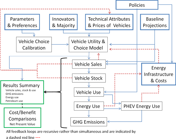
FIGURE H.1 Diagrammatic representation of the LAVE-Trans Model.
This report provides an overview of the LAVE-Trans model structure, explains how it functions, and provides instructions for operating it. Section H.2.2 provides an overview of the model structure and the components and how they are linked together. Section H.2.3 describes each component, including the key equations that control its operation. Section H.2.4 describes the inputs (parameters and data) that must be supplied to the model, and Section H.2.5 describes model outputs. Section H.2.6 is a brief users’ guide to executing a model run.
H.2.2 Model Structure
The LAVE-Trans model is an Excel spreadsheet model comprised of 25 worksheets. Figure H.1 illustrates the relationships between the major components of the model. The areas where exogenous inputs enter the model are shown as blue boxes. A relatively large amount of exogenous information is required to carry out a model run. Baseline projections of vehicle sales and energy prices are required to 2050. Technical attributes of advanced technology vehicles, including fuel consumption per kilometer, on-board energy storage, and retail price equivalent (RPE) at full scale and learning, must be specified for current and certain future years. Parameters that describe consumers’ willingness to pay for vehicles and
their attributes must also be provided. The model translates these into coefficients for the vehicle choice model. Capital, operating, and input costs of both electric, hydrogen, and natural gas infrastructure or alternative price projections must also be provided.
The model can be automatically calibrated to specified vehicle sales and vehicle use projections. At that point the Vehicle Choice model estimates the shares of ICE, HEV, PHEV, BEV, and FCV or CNG technologies for passenger cars and light trucks and for Innovator and Majority market segments. The market shares are multiplied by the passenger car and light truck sales totals in the Vehicle Sales worksheet. Sales are passed to the Vehicle Stock worksheet, which retires vehicles as they age and keeps track of the number of vehicles of each technology type by model year for every forecast year. Vehicle kilometers by age and vehicle type are calculated in the Vehicle Use worksheet. In the Energy Use worksheet, energy use is calculated for all but PHEVs by multiplying vehicle kilometers by the number of vehicles and by on-road energy consumption per kilometer. PHEV energy use, electricity and gasoline, is calculated in a separate worksheet. GHG emissions factors are applied to energy use in the GHG Emissions worksheet.
In a BAU run, the total passenger car and total light truck sales will exactly match the input projections. The technology and price assumptions of the BAU Case should match the baseline projection to which the model’s vehicle sales and vehicle use have been calibrated. Next, a Base Case, reflecting alternative technology and price assumptions can be run. In the Base Case, vehicle sales, vehicle use, energy use, and GHG emissions will change due to the new technology and price assumptions. Once a Base Case run has been made, it is transferred to the Base Case worksheet by clicking on a button in the Current Case worksheet. A policy run may then be created by specifying vehicle or fuel subsidies or taxes, exogenous investments in fuel infrastructure, or by changing assumptions about vehicle or fuel technologies. In a policy run, sales may be higher or lower than the Base Case, depending on the specific policy assumptions. The results of a policy case are stored in a Current Case worksheet, which also contains built-in graphical displays. The impacts of the Current Case relative to the Base Case are calculated in the Costs-Benefits worksheet. A standard set of tables and graphs summarizing the BAU Case, Base Case, and Current Case are stored in an Output worksheet.
There are several important feedback loops in the model. Feedbacks are recursive (with a 1-year lag) rather than simultaneous. This simplifies the solution of the model greatly but is also generally more representative of how changes can be made in the motor vehicle industry. Cumulative vehicle sales generate learning-by-doing effects that lower vehicle prices over time. Sales are accumulated in the Vehicle Sales worksheet, and learning effects are calculated there, as well. Current sales affect the availability of different makes and models, i.e., the diversity of choice available for both advanced and conventional ICE technologies. A diversity of choice metric is passed to the Vehicle Attributes worksheet. Current sales also affect next year’s vehicle prices via scale effects, also computed in the Vehicle Sales worksheet. Both learning and scale effects are passed to the Vehicle Production worksheet, where RPEs are calculated for each technology in each future year. These adjusted prices are then passed to the Vehicle Attributes worksheet.
Demand for electricity, hydrogen, and natural gas, plus exogenous assumptions about the supply of refueling/recharging infrastructure, are passed to the Fuel Input worksheet, where the quantities and costs of infrastructure are calculated. For hydrogen, these costs also depend on the model user’s assumptions about how hydrogen will be produced and delivered to vehicles in the future. These assumptions also affect the cost of hydrogen and its GHG emissions per kilogram. The availability of refueling/recharging infrastructure is passed to the Vehicle Attributes model and influences the choice among alternative technologies.
The following is a list of the model’s 25 worksheets along with a brief description of their functions:
a. Flow Chart—contains the diagram of the model structure shown in Figure H.1.
b. Scenario Assumptions—contains alternative data sets describing vehicle and fuel technologies, as well as a table in which the different data sets can be conveniently selected to construct fuel and
vehicle technology scenarios. Alternative social values for reducing petroleum use and GHG mitigation may also be selected.
c. Parameter Input—contains most of the key assumptions of the model that a user will want to change in creating a new run.
d. CO2 Cost—holds the alternative estimates of the social value of reducing carbon emissions from the U.S. government’s interagency assessment of the social costs of carbon (Interagency Working Group, 2010).
e. Hydrogen Stations—contains the multinomial logit model used to estimate a smooth transition from a user-specified initial distribution of types of hydrogen stations to a user-specified long-run configuration as a function of the total volume of hydrogen production for LDVs.
f. VISION—used storing output from the Argonne National Laboratory’s VISION model. The LAVE-Trans model can be forced to match the market shares of a VISION run. In that mode, it calculates the costs and benefits of achieving the particular VISION scenario.
g. Vehicle Attributes—contains the key vehicle attributes, by year, from 2010 to 2050. Most are derived from data contained in the Parameter Input worksheet.
h. Risk Groups—contains assumptions and calculations about innovators and majority adopters. At present these are the only two classes of consumers.
i. Choice Parameters—where the coefficients of the nested multinomial logit (NMNL) model for predicting choices among technologies are calculated.
j. Vehicle Production—where learning-by-doing, scale effects, and rates of exogenous technological progress are applied to the prices of technologies to estimate RPEs by year.
k. Vehicle Choice—the above factors come together to estimate market shares for each technology for new vehicles, as well as household’s decisions to buy or not buy a new vehicle in a given year. Consumers’ surplus is calculated here as well. Also calculated here are the cost components (i.e., cost of lack of fuel availability, cost of lack of diversity of choice, etc.) that also comprise the positive network externalities generated during the transition.
l. Vehicle Sales—the choices are applied to total vehicle sales (which will vary by time as the buy/no-buy decision changes each year) to produce estimates of sales by passenger cars and light trucks, by technology type and for innovators and majority. Also calculated in this worksheet are cumulative production, learning-by-doing, scale economies, and choice diversity.
Next come a series of large worksheets that depend on vehicle stock turnover.
m. Vehicle Stock—adds new vehicles to the existing fleet and scraps older vehicles by vintage. There are 10 tables (PC versus LT) × (five technologies).
n. Vehicle Use—multiplies kilometers per vehicle by vehicle age by the number of vehicles in the vehicle stock to estimate vehicle kilometers traveled (VKT) by vehicle type, technology type and 25 vintages. A rebound effect is built in to represent the tendency of vehicle use to increase when fuel cost per kilometer declines.
o. Energy Use—uses the vehicle efficiency estimates by vintage together with an on-road adjustment factor to estimate energy use by the same 250 categories for all years 2010 to 2050.
p. PHEV Energy—divides PHEV energy use into electricity and gasoline.
q. GHG Emissions—applies fuel specific well-to-wheel GHG factors to estimate emissions in CO2 equivalents, again for all vehicle types, technology types, vintages, and years.
r. Fuel Input—contains information about the capital, operating, and delivery costs of alternative LDV energy sources and their lifecycle GHG emissions.
s. Input USA—where the projections of U.S. vehicle sales by vehicle type and technology type are stored. In addition to vehicle projections there are U.S. VKT projections, energy price projections, value of time projections (related to income per capita) and demographic projections (e.g., numbers of households).
t. Input World—where the assumptions about the production of alternative energy vehicles outside of the United States are input. These projections are exogenous and never changed by the model.
u. Current Case—contains summaries of costs, GHG emissions, energy use, vehicle stocks, vehicle sales, and VKT for the current case running in the model. The energy efficiency of the on-road vehicle stock is calculated in this worksheet, as well as average GHG emissions rates. The Current Case can be stored in the Base Case worksheet by clicking on a button that executes a macro that copies it to that location.
v. Base Case—should reflect the same scenario assumptions about technologies and energy costs as the Current Case. The two cases will be compared in the Costs-Benefits worksheet.
w. Business as Usual Case—may be stored in the BAU worksheet; should reflect the assumptions of the vehicle sales and vehicle travel projections to which the model has been calibrated, for example, a Reference Case projection of the EIA’s AEO.
x. Costs-Benefits—Once a Current Case has been copied to the Base Case worksheet, changes to the model’s inputs and parameter assumptions create a new Current Case. Differences between the Base Case and the Current Case are calculated in the Costs-Benefits worksheet. Here one will find the infrastructure, vehicle and fuel subsidy costs, changes in consumers’ surplus, and societal benefits due to reductions in GHG emissions and petroleum use.
y. Output—contains a summary and comparison of the BAU Case, Base Case, and Current Cases, via a fixed set of tables and graphs.
H.2.3 Description of Model Components
In this section, the theory and equations of each key LAVE-Trans model component are presented and explained.
H.2.3.1 Vehicle Choice Model
Consumer demand is represented by a discrete choice, NMNL model, including a buy/no-buy choice. The buy/no-buy choice represents consumers’ decisions to buy a new motor vehicle or to use their income for something else. In each time period, each household is assumed to make a buy versus no-buy decision. This allows for a more complete estimation of consumers’ surplus effects, as well as allowing vehicle sales to increase or decrease in response to changes in policies or assumptions about technologies.
The vehicle choice model is a representative consumer model. Although it is desirable to segment the consumer market to reflect the heterogeneity of consumers’ preferences, this comes at a high price in terms of the complexity of the model and its input data requirements. In the LAVE-Trans model, the market is split into only two segments: innovators/early-adopters versus the majority. More complex market segmentation could be added in a subsequent model development effort, if warranted.
The LAVE-Trans NMNL model allows a variety of factors, Xij, including make and model diversity and fuel availability, as well as price, energy efficiency, and range to determine the utility, Ui, of each technology, i. Price is a special variable in the utility function, because its coefficient has units of utility per present value dollar. Thus, if the value of any attribute can be estimated in terms of dollars per unit of the attribute (e.g., present value dollars per MJ/km of fuel consumption), then its coefficient can be determined by multiplying the value per unit times the coefficient of price, βk (where k is an index of the technology class, or nest, to which alternative i belongs). In this way, every coefficient in Equation H.2 is a function of the sensitivity of utility to price.
![]()
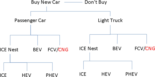
FIGURE H.2 Nesting structure of the LAVE-Trans model.
The NMNL model allows for some control over the patterns of substitution among vehicle technologies. In particular, vehicles within a given nest are closer substitutes for one another than they are for vehicles in a different nest.5 The nesting structure used in the model is shown in Figure H.2. The first level of choice is to buy or not to buy a new LDV. The second is the choice between a passenger car and a light truck. The third level is the choice between an ICE, a BEV, and an FCV. The model allows the user to substitute a CNG vehicle for the FCV, but the number of technology choices has been limited to five for the sake of simplicity. Within the ICE nest is the choice between a conventional ICE, an HEV, and a PHEV. The order of nesting does not signify a temporal sequence of choices. Rather, it orders choices from least price sensitive (buy versus no-buy) to most price sensitive (ICE, HEV, or PHEV) and attempts to group choices within a nest that are closer substitutes than choices within some other nest.
The ability to translate attributes into dollar values is useful for measuring the network externalities that arise in the transformation of the energy basis for motor vehicles. For example, increasing fuel availability by adding public recharging stations or hydrogen fueling stations will reduce fuel availability costs. This improvement in fuel availability can be translated into an indirect network externality and be given a dollar value per vehicle using the relationships in Equation H.2. Likewise, if an innovator purchases a novel technology vehicle, this generates benefits for subsequent purchasers increasing scale and learning-by-doing, bringing down the price of vehicles, and by reducing the risk perceived by the majority market segment.
Market shares depend on each alternative’s utility indexes, Uik. At the lowest level nests, the probability of choosing alternative i, given that a choice will be made from nest k, Pi|k, is given by the logit equation in which e is the base of the Naperian logarithms, and m indexes other choices in nest k.

_____________________________
5 More precisely, vehicles are more similar in their “unobserved attributes,” meaning attributes that are not included in the model. For example, the sound of an electric-drive vehicle will be different from that of an ICEV, and this may influence consumers’ choices.
The probability that a choice will be made from nest k depends on all the alternatives in nest k, as well as the utilities of all other nests at the same level. Let the measure of the utilities of all alternatives in nest k be represented by Ik, the “inclusive value” of nest j.
![]()
The probability of a choice being made from nest j is a logit function of the inclusive values of j and the other nests (indexed by k) at the same level as j.

In Equation H.5, β is the price coefficient for the choice among nests. The parameter A j reflects aspects of nest j that are common to all members of the nest. In the LAVE-Trans model, the A j parameters are generally set to zero, except at the level of choice between passenger car and light truck and buy versus no-buy. These coefficients are used to calibrate the choice model to a baseline sales forecast for passenger cars and light trucks. The procedure for calculating inclusive values can be used for any degree of nesting choices by simply passing inclusive values up to the next level.
The probability that technology i will be selected from nest j is the product of the probability of choosing nest j and the probability of choosing i, given that a choice will be made from nest j : Pij = Pi|j Pj. This relationship is repeated as one moves from the lowest nests up to the buy/no-buy decision.
The NMNL model also allows direct calculation of the change in consumers’ surplus due to changes in the prices and attributes of the choice alternatives. The change in consumers’ surplus per household between the base case and an alternative scenario can be calculated at the top of the nesting structure from the utilities of the buy and no-buy choices. The superscript 0 indicates the Base Case, and the superscript 1 indicates the Scenario Case, and β* is the price coefficient of the buy/no-buy choice.
![]()
H.2.3.2 Calibration of Choice Model Parameters
The following nine variables determine the market shares of the alternative advanced technologies:
1. Retail price equivalent (RPE),
2. Energy cost per kilometer,
3. Range (kilometers between refuel/recharge events),
4. Maintenance cost (annual),
5. Fuel availability,
6. Range limitation for BEVs,
7. Public recharging availability,
8. Risk aversion (innovator versus majority), and
9. Diversity of make and model options available.
NMNL models can be calibrated to the best available evidence on the sensitivity of consumers’ choices to vehicle prices and the value consumers attach to vehicles’ attributes, including range, fuel economy, performance, fuel availability, and diversity of choice. The procedure requires estimating the present dollar value per unit of the attribute, which can then be multiplied by the price coefficient to derive a coefficient that translates one unit of the attribute into a utility index. Each of the attributes and the method for estimating its NMNL model coefficient is considered below.
H.2.3.2.1 Diversity of Choice Among Makes and Models
Make and model diversity is represented in the vehicle choice model as the log of the ratio of the actual number of makes and models available, n, to the “full diversity” number, N, represented by the number of makes and models of the conventional technology available in the base year, ln(n /N) (for a derivation, see Greene [2001], pp. 21-22). This variable is then multiplied by a coefficient (e.g., a default value of 0.67 is used in most cases) that depends on the cumulative sales distribution across makes and models. The number of makes and models available in any given year can be determined by dividing total sales by the production volume at which full scale economies are achieved.6
H.2.3.2.2 Consumers’ Aversion to the Risk of New Technology
Consumers’ risk aversion to new technologies (the early adopter, early majority, and late majority phenomenon) is represented in a manner analogous to learning by doing. Innovators have a preference for novel technologies (a utility premium) that decreases with cumulative sales. The majority of the market may have an aversion for novel technologies (a negative utility) that decreases with cumulative sales. These are represented by exponential “cost” functions that enter into the consumers’ utility functions. Each group is assigned a monthly quantity to either avoid (+ cost) or gain (-cost) the opportunity to purchase a vehicle with novel technology. The monthly payments are discounted to present value assuming a certain length of loan or lease (e.g., 48 months) and annual real interest rate (e.g., 7 percent). A slope coefficient for the exponential function is estimated by specifying the cumulative sales point at which the risk or novelty value of the new technology will be reduced by half. The slope coefficient, b i, is the logarithm of 0.5 divided by the specified cumulative sales. Given the estimated present value, V i, for group i and slope coefficient, b i, the risk to majority buyers and the novelty value to innovators, vij, is a function of cumulative sales of technology j, Qj.
![]()
In the current version of the model, the market is divided into only two groups: innovators and the rest of the market represented by the majority. The percent of the market in each group can be specified.
_____________________________
6 This implies that the diversity of choice for the conventional technology is total sales divided by the same full scale production volume. For example, if conventional LDV sales are 15 million in the base year and the production level for full scale economies is 100,000, then the diversity measure would be N = 150 for conventional vehicles.
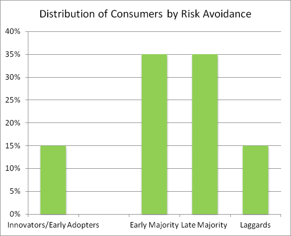
FIGURE H.3 Default distribution of consumers by aversion to risk of new products.
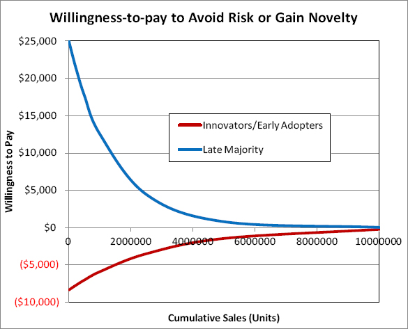
FIGURE H.4 Default willingness-to-pay functions for innovators/early adopters and majority.
H.2.3.2.3 Value of Energy Efficiency
The value of energy efficiency is represented by the present value of future fuel savings. The way consumers value future fuel savings is a largely unresolved issue, with the econometric evidence split roughly 50/50 between undervaluing versus accurately valuing or overvaluing (Greene, 2010). If consumers consider paying more up front for future fuel savings a risky bet, behavioral economics implies that consumers will undervalue future fuel savings by one-half or more (Greene, 2011). The LAVE-Trans model allows for different specifications of consumers’ valuation of future fuel costs within the context of discounting to present value. The following variables determine the present value of future fuel costs:
E = a vehicle’s energy efficiency in MJ/km,
P = the price of energy per MJ,
M0 = the vehicle’s annual kilometers when new,
L = the vehicle’s lifetime in years,
r = the consumers’ discount rate, and
δ = the rate of decline in vehicle use with vehicle age.
The present value of fuel costs is the integral over the vehicle’s lifetime of the instantaneous fuel costs.
![]()
In Equation H.8 it is assumed that the price of fuel over the life of the vehicle is constant. While this is certainly incorrect, it is consistent with rational expectations given fuel prices that follow a random walk (Hamilton, 2009). If the discount rate is set to zero and L is set to 3, for example, this formula becomes a 3-year payback formula. The term in square brackets is discounted vehicle travel, which is useful in estimating the value of other vehicle attributes, such as range.
The variable representing energy efficiency is energy cost per kilometer. The coefficient of vehicle energy cost per kilometer ($/MJ × MJ/km) is discounted lifetime kilometers (the term in square brackets in Equation H.8 multiplied by the price coefficient.
H.2.3.2.4 Value of Maintenance Costs
Maintenance costs are assumed to be incurred annually over the life of a vehicle. The vehicle attribute is defined as annual maintenance costs in dollars. Thus, the coefficient is discounted years of vehicle life multiplied by the price coefficient. Discounted years are equal to the term in square brackets of Equation H.9. The time horizon over which maintenance costs are discounted is allowed to be different from that for fuel costs to allow flexibility in representing consumer behavior.
![]()
H.2.3.2.5 Value of Range
The value (or cost) of range is calculated as the discounted present value of time spent refueling over the life of the vehicle. The range variable is defined as the time required per refueling (in hours), t r, multiplied by the value of time (in $/hr), v, divided by kilometers per tank of fuel or kilometers per charge. Thus, it is the inverse of range that determines the value of range. Kilometers per tank is calculated by multiplying usable energy storage in gallons of gasoline equivalent, q, times the number of MJ per gallon, c, and dividing by the vehicle’s energy efficiency in MJ/km, E. The denominator of the term in the righthand-most brackets of Equation H.10, cq /E, is what is usually defined as vehicle range: kilometers per tank or per charge. The cost of increased range falls inversely with range. On-board energy storage capacity and vehicle energy efficiency may change over time, as may the value of time and the time required to refuel. It is assumed that neither a fuel tank nor a battery will be completely exhausted before it is replenished. Energy storage capacities should, therefore, be specified in terms of usable energy storage rather than total energy storage. In Equation H.10, the term in round brackets is the coefficient of range, while the term in {} brackets is the range variable. The coefficient of range is discounted lifetime kilometers multiplied by the price coefficient. The range variable is the value of time spent refueling per kilometer of vehicle travel.
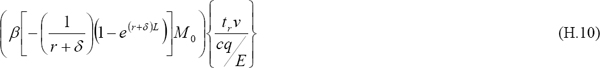
Equation H.10 does not accurately represent the recharging cost for PHEVs. For PHEVs, the time required to fully recharge a battery is likely to be hours, but the driver will not stand by idly while the vehicle charges. The EV’s problem is a combination of limited range and long recharge time. In the LAVE-Trans model, Equation H.10 is used only to account for the time require to plug and unplug the vehicle. It assumed that during recharge the driver is able to use his or her time productively in other pursuits and that, therefore, the cost is zero. On the other hand, the combination of long recharge time and short range will make the plug-in vehicle unable to accommodate motorists’ desired travel on those days when the desired travel exceed the vehicle’s range. We use a different method, described in Section H.2.3.2.8, to account for those costs.
H.2.3.2.6 Value of Fuel Availability
The value of fuel availability is a key component of transition costs; it is the fuel half of the “chicken or egg” problem for alternative fuels. Despite some very good recent research (e.g., Nicholas et al., 2004; Nicholas and Ogden, 2007; Ogden and Nicholas, 2010; Melaina and Bremson, 2008), quantifying the value of fuel availability remains a challenge. The estimate used here begins with a measure of the extra time required to access fuel in a metropolitan area as a function of the ratio of the number of stations offering the alternative fuel to a reference number of gasoline stations. The fuel availability variable in the Vehicle Attributes spreadsheet is that ratio. The method is based on simulation modeling by Nicholas et al. (2004) and was used in the Department of Energy’s modeling of market transitions to hydrogen (Greene et al., 2008).
The coefficient of the fuel availability variable is the coefficient of vehicle price times discounted lifetime kilometers (the term in square brackets in Equation H.8) times a multiplier that represents the ratio of the total cost of fuel availability to the cost of access time within one’s own metropolitan area. This multiplier, which is given a default value of 3, represents the extra value of regional and national fuel availability, as well as the added fear of risk of running out of fuel. This is generally consistent with the results of Melaina’s (2009) stated preference analysis of consumers’ preferences for refueling availability, which found very roughly comparable values for availability in (1) one’s metropolitan area, (2) regionally, and (3) nationally.
The fuel availability term in the choice model combines the effects of range, R, and fuel availability, fj = nj /N0, where nj is the number of stations offering fuel for technology j and N0 is the reference number of stations (i.e., the number of gasoline refueling stations in the base year). As range increases, fuel availability decreases in importance because the number of refueling events decreases. In Equation H.11, Bf is the coefficient of the fuel availability variable (discounted lifetime kilometers multiplied by the price coefficient), w is the value of time in $/hour, C is a coefficient from the Nicholas et al. (2004) model relating the number of stations to access time, and a is the second coefficient of that model.
![]()
The term in square brackets in Equation H.11 is the extra access time required per refueling event, which is converted into a dollar value by the value of time, w. The 1/R term adjusts the coefficient B f for changes in vehicle range over time due to improved energy efficiency or energy storage.
Representing fuel availability as a ratio to a reference number of outlets is an approximation of a much more complex process. In the earliest stages of infrastructure evolution, stations are likely to be placed in clusters near concentrations of FCV owners; clustering will be a self-reinforcing process. Ogden and Nicholas (2010) estimated that in the Los Angeles, California, area, as few as 42 stations could provide one station that is within 2.6 minutes of home for clustered FCV owners. If stations were distributed by population density instead, it would require 4 to 15 times as many stations, 1.5 to 3 percent of the number of gasoline stations in the Los Angeles basin.
H.2.3.2.7 Value of Public Recharging
The value of the availability of public recharging to BEVs is a function of the present value of full availability of public recharging versus none, based on an analysis by Lin and Greene (2011a). That study derived a value of public recharging as a function of the number of days in a year an EV would not be able to satisfy typical kilometers traveled and the cost of renting a vehicle with unlimited range for those days. Let V be the present value of unlimited public recharging, f the availability of public recharging relative to the availability of gasoline stations, and β be the coefficient of vehicle price, and b be a slope coefficient. The value of public recharging is given by Equation H.12. It increases from 0 to approach V as f increases from 0 to 1.0.
![]()
This method is very approximate and should be improved. In particular, the value of public recharging should also depend on vehicle range.
The value of public recharging to PHEVs is estimated by an equation identical in form to Equation H.12, also based on the analysis by Lin and Greene (2011a). The price coefficient, β, value, V, and slope b are specific to PHEVs, however.
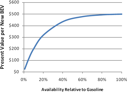
FIGURE H.5 Estimated present value of public recharging for a new battery electric vehicle.
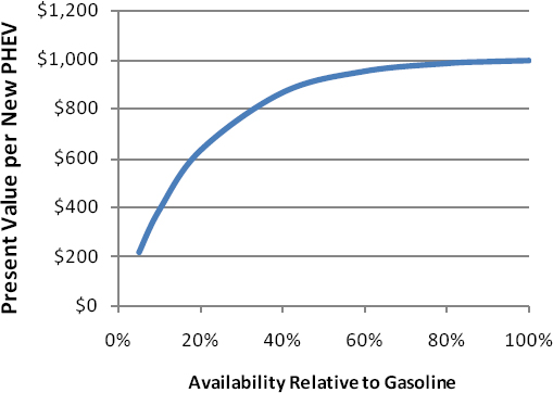
FIGURE H.6 Estimated present value of public recharging for a new plug-in hybrid electric vehicle.
H.2.3.2.8 Value of Range Anxiety
Range anxiety typically describes the fear of being stranded that the owner of a vehicle with limited range, long recharging time, and limited availability of public recharging may experience. The perceived cost of this form of range anxiety is likely to vary greatly from individual to individual and over time, as well, as drivers learn about their vehicles. In the LAVE-Trans model range anxiety is defined differently as the loss of utility due to a vehicle’s inability to be used for more than a certain number of miles per day. Range anxiety declines exponentially at a rate b from a theoretical maximum value at zero range, X, to asymptotically approach zero as range R goes to infinity. Once again, β is the coefficient of price. The values shown in Figure H.7 were taken from Lin and Greene (2011b), who calculated the number of days a vehicle with range R would be unable to accomplish the daily driving pattern of typical U.S. drivers. Lin and Greene (2011b) suggest a daily penalty of $15 to $30, which is typically less than the cost of renting a vehicle to accomplish the usual driving, because motorists have other options, especially if the household owns more than one vehicle.
![]()
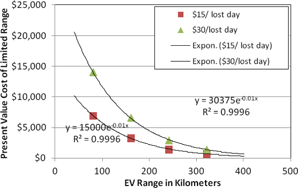
FIGURE H.7 Present value cost of limited range (range anxiety) for a new BEV.
H.2.3.3 Vehicle Sales and Vehicle Production
Sales of alternative vehicles generate positive feedback for these new technologies by inducing learning by doing, scale economies, greater diversity of choice in the number of makes and models, and by reducing majority consumers’ aversion to risk. Sales by vehicle type (passenger car versus light truck) and by technology type are estimated by multiplying total sales by the shares predicted by the NMNL vehicle choice model.
Base Case sales are calibrated to exactly match exogenous total LDV sales by means of year-specific constants for the buy/no-buy choice. Similarly, the shares of passenger cars and light trucks are individually matched to the exogenous Base Case projection by calibrating a constant term for the NMNL car versus truck choice for each year. This insures that for the Base Case only, total sales as well as car and light truck sales exactly match the exogenous projection. In policy scenarios, changes in vehicle technology and new policies (e.g., vehicle or fuel taxes or subsidies) can not only change the market shares of vehicle technologies but the split between passenger cars and light trucks and total sales, as well. The calibration constants are calculated iteratively by first estimating an initial value, substituting that value into the NMNL choice model, and then recalculating a new value. Iteration is necessary because the calibration constants affect shares, which in turn determine sales, and sales affect the utility indexes for vehicles via fuel prices, learning by doing, scale economies, make and model diversity, and fuel availability. Let IC and SC be the inclusive value and Base Case market share, respectively, for passenger cars, and IT and ST are the corresponding values for light trucks. The initial estimate of the light truck constant term is the following (in which the superscript 1 indicates the first iteration).
![]()
When the calibration constant is substituted in the vehicle choice equation, it results in different market shares and, therefore, sales for cars and light trucks, which affects their prices and other attributes via the feedback mechanisms of learning, scale economies, etc. This in turn affects the inclusive values, resulting in a different estimate for the constant term via Equation H.14. The process is repeated until the constant terms are determined to at least four-digit accuracy. A similar process is used to simultaneously estimate the year-specific constant terms for the buy/no-buy choice. Typically, convergence is achieved over the 40-year forecast horizon in about 10 iterations.
Via several feedback mechanisms, vehicle sales affect future vehicle prices, numbers of makes and models from which to choose, and fuel availability. The key mechanisms affecting the prices of new technologies during the early stages of a transition are learning by doing and scale economies. Learning by doing is represented by declining costs as a function of cumulative production, Q, relative to an initial reference level, QR. The rate of learning, or progress ratio, á, represents the impact of a doubling of cumulative output on cost. Let P (Q0) represent the RPE at cumulative production Q0, then the RPE at cumulative production level Q > Q0 is given by Equation H.15.
![]()
This formulation has a significant drawback, namely that costs can decline to zero as cumulative output approaches infinity. The LAVE-Trans model limits the reduction in cost so that costs converge to the long-run RPE estimates provided by model users.
Scale economies are represented by a scale elasticity, c, which is the exponent of the ratio of production volume in a given period, q, to the ideal production volume, q *, at which full-scale economies are realized. RPE is equal to the ideal RPE, P *, times the ratio q /q * raised to the c. Values of the scale
elasticity, c, are often in the vicinity of -0.25, implying that a doubling of volume reduces costs by about 15 percent. Once q >= q *, q is set = q * so that the scale elasticity factor will never be smaller than 1.0.
![]()
Technological progress is determined by user-specified prices, energy efficiencies, and other attributes, which are key exogenous inputs to the model. The technologically achievable price at time t, P t, is defined as the RPE that could be achieved at full-scale and fully learned production. The user must specify the technologically achievable prices, energy efficiencies, and other vehicle attributes for 2010, 2015, 2020, 2030, 2040, and 2050. Technologically achievable prices and attributes for intervening years are estimated by linear interpolation. Attributes are assumed to be achieved regardless of current or cumulative sales. Prices must be driven down by learning and scale economies.
Using the above framework, the RPE of an advanced technology vehicle at any given time is the product of the technologically achievable price, Pt, times the technological progress, learning by doing, and scale economy functions.

H.2.3.4 Vehicle Stock
Vehicle stock, Scimt, is the number of vehicles of class c (passenger car, light truck) and technology type i, manufactured in model year m, in operation in calendar year t. The default survival functions for cars and light trucks are taken from NHTSA (2006). Alternatively, a three-parameter scrappage/survival function can be used to retire a fraction of the vehicle stock each year as vehicles age. Let Ri (a) be the scrappage rate function for vehicles of technology type i and age a = t – m, and Ai0, Ai1, and Ai2 be parameters of the scrappage function. The scrappage rate is the fraction of vehicles of age a – 1 in year t – 1 that are retired (scrapped) in year t. The fraction of vehicles surviving to age a is 1 -Ri(a).
![]()
The number of a-year-old (a = t – m) vehicles surviving from year t to year t + 1 is given by Equation H.19.
![]()
Vehicle stock accounts are kept for 25 ages (0-24); vehicles older than 24 years are combined into a single >25 category and scrapped at a constant rate equal to 1/Ai0.
H.2.3.5 Vehicle Use and Energy Use
Vehicle use, Vi (a), is assumed to be primarily a function of vehicle technology and vehicle age, but it also varies with energy efficiency to account for the rebound effect and varies with growth in the
TABLE H.4 Parameters for National Highway Traffice Safety Administration Cubic Equation for Vehicle Use as a Function of Age
| C3 | C2 | C1 | C0 | ||||||
| Car | 0.36721 | -13.2195 | -232.85 | 14476.4 | |||||
| Truck | 0.68064 | -22.8448 | -238.55 | 16345.3 | |||||
vehicle stock. Vehicle use as a function of age for passenger cars and light trucks is based on NHTSA (2006), which fitted cubic polynomials to annual mileage at 1-year age intervals. Annual miles for vehicle type i (passenger car, light truck) is given by Equation H.20.
![]()
The parameter values derived by NHTSA are shown in Table H.4. Vehicle miles are converted to kilometers by multiplying by 1.609. The resulting typical curves for passenger cars and light trucks are shown in Figure H.8. The same parameters may be used for every vehicle technology, or the user may specify different annual usage rates for different vehicle technologies. However, this should be done with caution. In the current version of the model, changing usage rates could profoundly affect total vehicle travel in scenarios in which low-usage vehicles become predominant. If a lower than average usage rate is specified for BEVs, a fraction of the reduction in travel will be shifted to other vehicle technologies. When a BEV’s range and recharging limitations make it unable to perform a consumer’s typical, desired daily travel, the consumer may (1) forego the travel or take a shorter trip, (2) shift the travel to another vehicle already owned, or (3) purchase or rent an additional vehicle. The model user can specify percentages for each option. The percentage allocated to option 1 will result in a decrease in total travel.
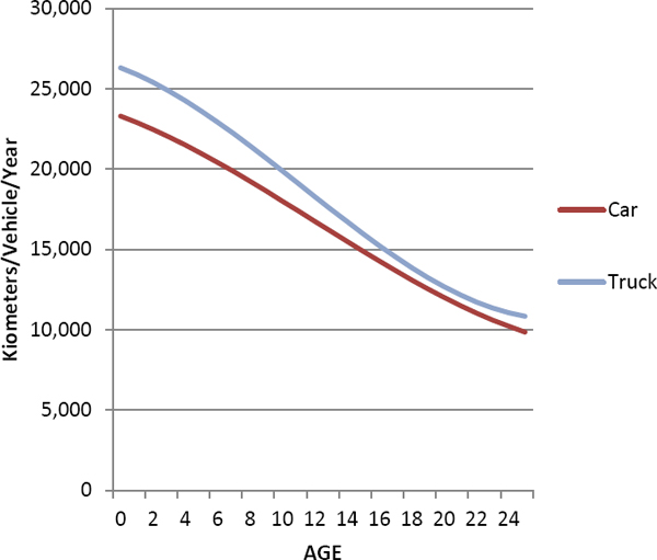
FIGURE H.8 Annual vehicle kilometers traveled by age of vehicle.
The percentages specified for options 2 and 3 will be allocated to other vehicle types. At present, the model does not allow vehicle sales to increase to accommodate option 3. For example, suppose a model user specified that 10 percent of the vehicle miles that could not be performed by a BEV would be foregone, 60 percent would be shifted to other vehicles, and 30 percent would be accommodated by the purchase of additional vehicles. If EVs comprised 10 percent of vehicles in use and were used on average 30 percent less than other vehicle types, there would be a 1.2 percent reduction in total VMT, and 1.8 percent of the travel would be shifted to the remaining 90 percent of vehicles, increasing their rates of use by 2 percent.
H.2.3.5.1 Adjustment for Changes in the Size of the Vehicle Stock
Because the vehicle choice model includes the option to buy or not to buy a new vehicle that depends on the attractiveness of new vehicles relative to other consumer goods, total LDV sales and stock size may change from one scenario to another. If annual kilometers traveled per vehicle (by age) were constant, then vehicle travel would increase approximately in proportion to the size of the vehicle stock. In fact, because the United States now has more motor vehicles than licensed drivers, vehicle travel is relatively insensitive to increases in the number of vehicles available for use. For example, Greene (2012) found that a 10 percent increase in number of LDVs in the United States would lead to only a 2 percent increase in total VKT in the long run.7 Let the elasticity of total VKT with respect to the size of the vehicle stock be η. The effect of a change in the size of the vehicle stock in year t in scenario s, Sti, compared to the stock in year t in the base case, StB, on annual kilometers by a vehicle of age a in year t, Vats, is shown in Equation H.21.

Thus, if the vehicle stock in a given scenario increases by, say 10 percent relative to the Base Case, annual kilometers per vehicle will decrease by 7.34 percent, resulting in an increase of total vehicle kilometers by a factor of (1.1) × (0.9266) = 1.019, or about 2 percent.
H.2.3.5.2 Adjustment of VKT for Changes in Fuel Cost per Kilometer
Adjusting vehicle travel for changes in the cost of energy per mile, also known as the “rebound effect,” is accomplished in two steps. In the first step, VKT per vehicle by year and vintage is adjusted relative to the base year of 2010. Let pit be the price of energy for a vehicle of technology type i in year t, and Ecimt be the rate of energy consumption per kilometer for a vehicle of class c, technology i, model year m, in year t. Let ã be the rebound elasticity, the percent change in vehicle travel for a percent change in energy cost per kilometer. The first adjustment factor, k1, is the energy cost per mile in year t relative to the energy cost per mile in the base year, raised to the rebound elasticity.
![]()
_____________________________
7 This result pertains to models in which the sensitivity to fuel cost per mile was allowed to vary over time as a function of per capita income.
The elasticity of vehicle use with respect to fuel cost per kilometer of travel determines the percent change in travel per vehicle for a 1 percent change in fuel cost per kilometer. The default value, which may be changed by the model user, is –0.1, implying a 1 percent increase in travel for a 10 percent reduction in fuel cost per kilometer.
The second adjustment factor, k2t, is the ratio of total projected light-duty VKT from the exogenous AEO forecast, VAEO,t, relative to the model’s initial estimate of VKT for the BAU Case, V* BAU. Multiplying the model’s BAU VKT estimate by this factor insures that total VKT in the BAU Case will match the AEO projection in each forecast year.
![]()
This parameter ensures only that travel in the BAU Case matches the AEO projection. When assumptions about vehicle energy efficiency or cost or other variables are changed in a Base Case or Current Case, VKT will, in general, differ from the AEO projection. In particular, if vehicle efficiency improves and purchase prices decline, vehicle travel will increase due to the rebound effect and the increased number of vehicles on the road.
Energy use for all vehicles, Zcimt, is the product of vehicle stock, Scimt, vehicle use, Via, and vehicle fuel consumption, Ecim, divided by 1,000,000 so that the units are terajoules per year.
![]()
H.2.3.5.3 PHEV Energy Use
For PHEVs, energy use must be divided between electricity and gasoline. This is done by multiplying total energy use assuming the vehicle is operated entirely in charge-sustaining mode times the share of kilometers traveled in charge depleting mode, sd, times the relative energy consumption in charge-depleting mode compared to charge-sustaining mode, rd. The relative energy use is calculated as the ratio of the energy efficiency in charge-depleting mode divided by energy efficiency in charge-sustaining mode.
![]()
Gasoline energy use is then calculated as the product of total energy use assuming 100 percent charge depleting operation times 1 minus the share of kilometers in charge-depleting mode.
![]()
H.2.3.6 GHG Emissions
GHG emissions are calculated by multiplying time-dependent emissions coefficients, git, times the quantity of energy used, Zcimt. For PHEVs, two calculations are made, one for electricity consumption and another for gasoline consumption. Different emissions scenarios can be constructed by selecting alternative emissions coefficients for gasoline, electricity, hydrogen, and natural gas.
The GHG emissions of gasoline are computed as a weighted sum of its blend components’ GHG emissions rates. Let si be the share of fuel type i (i = conventional gasoline, corn-based ethanol, cellulosic ethanol, drop-in pyrolysis biofuel, coal-to-liquid gasoline, gas-to-liquid gasoline), and let gi be its
estimated well-to-wheel emissions rate in kilograms of CO2 per gasoline gallon equivalent energy. The GHG emissions rate of gasoline, g, is given by the following:
![]()
One of two scenarios can be selected for GHG emissions from electricity use. For the United States the GHG scenarios are based on the Reference Case and the Low Carbon Case of the GHG Price Case projections for the U.S. electricity grid of the EIA AEO 2011 extrapolated from 2035 to 2050.
Three alternative scenarios can be used for GHG emissions from hydrogen use. In all cases, emissions are assumed to be 11.44 kg CO2 per gge until hydrogen production reaches 6,000 metric tons per day (tpd; approximately enough to fuel 6 million vehicles). In a low-cost hydrogen case, no sequestration is assumed, and based on a mix of 25 percent distributed natural gas reforming, 25 percent coal gasification without CCS, 25 percent central natural gas reforming without CCS, and 25 percent biomass gasification without CCS, an emission factor of 12.2 kg/gge is used. A carbon sequestration case adds CCS to central coal and natural gas production but not distributed natural gas or central biomass, resulting in an emissions factor of 5.1 kg/gge. A low-CO2 case assumes only 10 percent distributed natural gas reforming, 40 percent central natural gas reforming with CCS, 30 percent biomass gasification without CCS, and 20 percent emission-free electricity (e.g., wind) for electrolysis, resulting in an emissions factor of 2.6 kg/gge.
H.2.4 Energy Infrastructure, Prices, and GHG Emission Rates
The costs of fuel supply infrastructure are estimated for electricity, hydrogen, and CNG. A distinction is also made between infrastructure necessary to support sales of vehicles and infrastructure added by public policy to increase fuel availability beyond the minimum necessary to support the stock of vehicles on the road. A model user may specify a fixed amount of infrastructure (or fuel supply) to be added as vehicles are sold and also the quantities and types of infrastructure deployed by subsidies or mandates.
H.2.4.1 Hydrogen
The hydrogen production and dispensing submodel estimates the number of hydrogen stations by type of station, the current price of hydrogen, and the average GHG emissions per kilogram of hydrogen used. For each hydrogen vehicle sold, it is assumed that enough fuel to operate the vehicle will be supplied and that only enough stations to provide that fuel will be constructed. The model user may require additional stations to increase fuel availability, but any additional stations will be fully subsidized (by government or industry).
The flow of the hydrogen production and delivery model is diagrammed in Figure H.9. The input data that define a hydrogen scenario consist of (1) long-run, high-volume hydrogen production costs,8 (2) GHG emissions per gallon of gasoline equivalent energy, and (3) target production process shares, all by production process and for the years 2010, 2020, 2035, and 2050 (e.g., Table H.5).
_____________________________
8 A future version of the model will build up these estimates from data on capital, operating and feedstock requirements and costs, as well as required returns on investment.
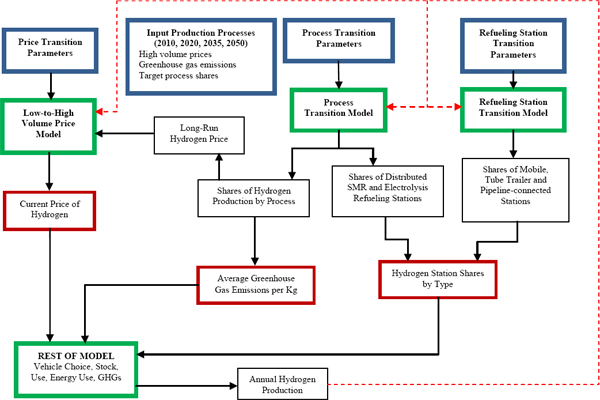
FIGURE H.9 Flow chart of hydrogen production and delivery model.
In the LAVE-Trans model hydrogen may be produced by the following eight processes:
1. Distributed natural gas reforming,
2. Distributed grid electrolysis,
3. Central coal gasification without CCS,
4. Central coal gasification with CCS,
5. Central natural gas reforming without CCS,
6. Central natural gas reforming with CCS,
7. Central biomass gasification without CCS, and
8. Central biomass gasification with CCS.
However, the processes chosen to produce hydrogen and the cost of hydrogen are not independent of the scale of hydrogen production. Early on, when production volumes are low, distributed production and distribution from central plants by mobile refueling units or tube trailers are likely to predominate. Later, as hydrogen production reaches thousands of tons per day, production is likely to favor more efficient central plants connected via pipeline to refueling outlets.
The process transition model makes a smooth transition from the initial production processes specified to the future year production processes specified by the user, as a function of the volume of production. The calculations of process shares, average costs, and average GHG emissions are carried out in three steps. First, production process shares for the intervening years are linearly interpolated between the specified years. Second, the process transition parameters are used to calibrate a logistic function of
TABLE H.5 Illustrative Assumptions for Production Shares by Process, GHG Emissions Rates and Long-Run Costs of Hydrogen
| Process | Production Shares | Greenhouse Gas Emissions (kg/gge) | Delivered Costs of Hydrogen ($/kg) | |||||||||
| 2010 | 2020 | 2035 | 2050 | 2010 | 2020 | 2035 | 2050 | 2010 | 2020 | 2035 | 2050 | |
| Distributed NG reforming | 50% | 50% | 25% | 25% | 11.44 | 11.44 | 11.44 | 11.44 | $3.49 | $3.60 | $3.90 | $4.20 |
| Distributed grid electrolysis | 0% | 0% | 0% | 0% | 35.44 | 35.44 | 35.44 | 35.44 | $5.76 | $5.38 | $5.54 | $5.69 |
| Central coal gasification without CCS | 0% | 0% | 0% | 0% | 25.81 | 25.81 | 25.81 | 25.81 | $3.81 | $3.82 | $3.84 | $3.85 |
| Central coal gasification with CCS | 0% | 0% | 25% | 25% | 5.24 | 5.24 | 5.24 | 5.24 | $4.46 | $4.46 | $4.48 | $4.49 |
| Central NG reforming without CCS | 50% | 50% | 0% | 0% | 11.46 | 11.46 | 11.46 | 11.46 | $3.28 | $3.36 | $3.69 | $4.01 |
| Central NG reforming with CCS | 0% | 0% | 25% | 25% | 3.64 | 3.64 | 3.64 | 3.64 | $3.55 | $3.63 | $3.96 | $4.28 |
| Central biomass gasification without CCS | 0% | 0% | 25% | 25% | 0.20 | 0.20 | 0.20 | 0.20 | $4.09 | $4.09 | $4.09 | $4.09 |
| Central biomass gasification with CCS | 0% | 0% | 0% | 0% | –21.73 | –21.73 | –21.73 | –21.73 | $4.74 | $4.73 | $4.73 | $4.73 |
the annual volume of hydrogen production. This function is bounded by zero and 1, and predicts the degree to which the transition from initial production methods to the user-specified shares for future years has been accomplished. The process transition parameters consist of two points on the logistic curve, e.g., fractions of the transition, f1 and f2, accomplished at corresponding production volumes v1 and v2. These define a two-parameter logistic function of the volume of production.
![]()
The logistic curve is calibrated such that 70 percent of the production occurs at the 2010 shares when volumes are below 3,000 tpd, 50 percent is at the initial shares, and 50 percent at the interpolated scenario shares when production reaches 6,000 tpd, and only 30 percent occurs at the initial shares when production reaches 9,000 tpd. The logistic function can be recalibrated by specifying different percentages for the production volumes. Figure H.10 illustrates a conversion of processes calibrated to a 50 percent conversion at 6,000 tpd and 30 percent by 9,000 tpd.
The transition function, f (v), is used to calculate a weighted average of the initial 2010 production shares and the interpolated shares. Let si0 be the initial share (at t = 0) of production process i, and let σit be the linearly interpolated, user-specified share for year t. The actual share for year t, sit, is the following:
![]()
The third step uses the volume-dependent production shares from step two to calculate weighted average, per kilogram GHG emissions and long-run hydrogen prices.
Short-run, or current year, hydrogen prices are a function of the current hydrogen production volume. If production is less than 60 tpd, the price of hydrogen is set at $10 per kg. If production exceeds 6,000 tpd, the cost is equal to the long-run price, calculated as described in the preceding paragraphs. For production volumes between 60 and 600 tpd, the price of hydrogen is given by a power function of the production volume in the current year t, q t,
![]()
where a0t and a1t are time-dependent constant terms calibrated to the point ($10, 60 tpd) and (pt, 6,000 tpd), where pt is the long-run price for year t as estimated by the Process Transition submodel.
The types and number of hydrogen refueling outlets are partly determined by the production processes and partly by other assumptions specified by the model user. For subsidized stations, the user specifies the number of stations of each type for all station types. For stations added as a function of the demand for hydrogen by fuel cell vehicles on the road, the percentages that are distributed stations are determined by the production process shares, while the percentages of stations of other types are determined by the Refueling Station Transition submodel.
The model user specifies the types of stations that will be built and their capacities and utilization rates. Five types of hydrogen stations can be specified as follows:
1. Mobile refueling units,
2. Stations serviced by tube trailers carrying liquefied hydrogen,
3. Distributed steam methane reforming,
4. Distributed electrolysis, and
5. Stations connected by pipeline to centralized production plants.
Given the total demand for hydrogen in year t, the minimum number of stations (not including subsidized outlets) is computed as follows. Let Et be the total estimated hydrogen demand based on the existing stock of hydrogen vehicles and their annual use and energy efficiency. Let s it be the share of hydrogen assumed to be supplied by stations of type i in year t, let c it be their specified capacity, and u it their specified utilization rate. The minimum number of stations of type i in year t is calculated by Equation H.31.
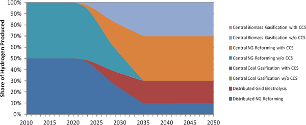
FIGURE H.10 Illustration of a transition from initial to high volume hydrogen production processes.
![]()
The demand for hydrogen vehicles in year t depends on fuel availability in year t – 1, and so it is not affected by stations added to supply vehicles sold in year t.
The shares of distributed steam methane reforming and electrolysis stations are also production method shares and are, therefore, specified when production methods are determined in the process transition model. The remaining three station types may be matched with any of the centralized production methods, and so the shares of these types of stations must be specified separately by the model user. These three station type shares are calculated as a function of the total volume of hydrogen production in the Refueling Stations Transition submodel. The share of station type i, s i, is given by a multinomial logit function of the total volume of hydrogen production in year t, qt.

This model is calibrated to user-specified shares at two different values for the total hydrogen production. This gives six data points from which the six model parameters can be calibrated. For example, if the initial shares are 95 percent mobile, 2 percent tube trailer supplied, and 3 percent connected to pipeline, while the shares at 30,000 tpd hydrogen production are 40 percent mobile, 10 percent tube trailer supplied, and 50 percent pipeline, then the predicted transition would be as illustrated by Figure H.11.
The number of stations of each type is the sum of those constructed to provide the minimum amount necessary to fuel the existing stock plus subsidized infrastructure added to increase fuel availability.
The cost of the additional subsidized stations is assumed to be borne either by hydrogen supplying companies or by the government, or both, and therefore does not affect the market price of hydrogen. It is, however, counted as a social cost of the transition.
H.2.4.2 Natural Gas
Natural gas infrastructure is handled in the same way as hydrogen infrastructure, except that it is much simpler. Because natural gas is already nearly ubiquitous, there is no need to model alternative production processes for natural gas. Only one type and size of natural gas refueling station is represented. Like the modeling of hydrogen, sales of natural gas vehicles automatically induce a sufficient number of natural gas stations to refuel the vehicles on the road. Additional natural gas stations can be specified to increase fuel availability, and these stations are assumed to be subsidized either by the government or fuel suppliers, or a combination of the two. The capital costs of natural gas stations are accounted for separately so that they can be tracked.
H.2.4.3 Electricity
Infrastructure for EVs is divided into the following three categories:
1. Level 2 home chargers,
2. Level 2 public chargers, and
3. Level 3 public chargers (or DC fast chargers).
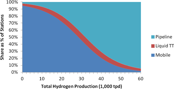
FIGURE H.11 Sample evolution of hydrogen station type shares as market expands.
The model user must specify how many of each type will be installed per PHEV sold and per BEV sold. For example, one might assume one level 2 home charger, 0.1 public level 2 chargers, and 0.01 public level 3 chargers per BEV. The number of public level 2 and level 3 chargers per PHEV may also be specified. Different ratios of chargers to vehicles may be specified for 2010, 2030, and 2050; ratios for intervening years are linearly interpolated. The total number of chargers of each type is equal to the number of BEVs and PHEVs on the road times the assumed numbers of chargers per vehicle, summed over vehicle technology types. The user may also specify charger costs for the years 2010, 2030, and 2050. Intervening year costs are linearly interpolated. The infrastructure capital cost in year t is the product of the cost per charger times the change in the number of chargers from year t – 1 to year t. If the number of chargers decreases from t – 1 to t, the capital cost for year t is zero.
The capital costs of home chargers are assumed to be paid for by the customer and included in the purchase price of an EV. The cost of public chargers is not added to the cost of grid-connected vehicles—it may or may not be included in the cost of electricity. If it is not included in the cost of electricity, the cost of public chargers is assumed to be a subsidy. In either case, infrastructure costs are accounted for and reported separately so that they can be tracked.
H.2.5 Policy Options
The LAVE-Trans model allows easy implementation of several policies that are designed to promote low-GHG emitting and high-fuel-efficient vehicle technologies, including feebates, an indexed highway user fee and fuel taxes. These policies are in addition to subsidies or mandates for vehicles or fuels.
H.2.5.1 Fuel Tax
Optional fuel taxes (e.g., $/gge) are calculated as the social cost of GHG emissions and oil dependence per unit of energy use by energy type. The model user can specify the cost of per unit of emissions ($/mmtCO2e) from four predefined scenarios. The current version of the model only defines one scenario for the cost of oil dependence ($/barrel).
H.2.5.2 Feebates
Feebates are fiscal policies that provide rebates to the purchase of new vehicles with low-GHG emissions/high energy efficiency and charge fees for the purchase of new vehicles with high-GHG emissions/low energy efficiency. Two feebate schemes are implemented. FeebatesA is designed to reflect social willingness to pay for GHG and petroleum reduction. First, for each vehicle technology, its lifetime GHG emissions and petroleum use are calculated, as well as corresponding social cost of emissions and oil dependence. Then, the value of fees or rebates for a technology is the difference between the lifetime social cost associated with this technology and the sales weighted average social cost for all technologies. FeebatesB, on the other hand, is designed to reflect fuel costs that are not considered by consumers when making purchase decisions. Uncounted lifetime fuel costs for each technology are calculated, and the value of fees or rebates is the difference between a technology’s uncounted fuel cost and the sales weighted average of uncounted fuel costs.
In the case that a fuel tax is also selected by users as one policy implemented in the model, the model will adjust the value of feebates by only considering social cost of GHG emissions and oil dependence that is not included in the fuel tax. Note that consumers are assumed to undervalue fuel costs (the payback period and discount rate can be specified by model users). Thus, the fuel tax accounts for that portion of the full social costs of GHG emissions and petroleum not included within the consumers’ payback period. The remainder of social cost is reflected in the feebates so that the combined effect of the feebates and fuel taxes equals and does not exceed the vehicle’s total private and social costs.
H.2.5.3 Indexed Highway User Fees
With the increase of vehicle energy efficiency, revenue from highway users collected via motor fuel taxes will decline because the existing taxes levied per unit of energy used are fixed (excise taxes). The model allows implementation of an indexed highway user fee for all fuels by scaling up current gasoline tax over time when fleet energy efficiency increases. Let q be the initial highway user fee and e be fleet average energy efficiency (e.g., MJ/km). If q0 is the initial rate and e0 is the initial energy efficiency, the tax rate in year t depends on the energy efficiency in year t, et, as follows:
![]()
H.2.6 Outputs
A model run produces estimates of vehicle sales and stocks by technology type, vehicle use, energy use by vehicle and energy types, GHG emissions and petroleum use by technology type, infrastructure costs, costs of explicit and implicit subsidies, and the impacts of technology and policy changes on consumers’ surplus.9 It is expected that a base case incorporating assumed changes in vehicle and fuel technologies will be run first, followed by a policy case that includes additional actions to increase the uptake of low carbon and low petroleum technologies, thereby generating societal benefits in the forms of reduced petroleum consumption and GHG emissions. Five spreadsheets hold the resulting projections.
The Current Case spreadsheet contains summary calculations for the data and parameters currently active in the model. It includes the following tables and associated graphs:
_____________________________
9 Consumers’ surplus is a monetized measure of consumer well-being, or satisfaction. It represents the economic value consumers perceive in a particular state of affairs.
1. Costs,
2. Greenhouse gas emissions and rates of GHG emissions by vehicle technology and energy type,
3. Energy use by vehicle technology and energy type,
4. Vehicle stock by technology type,
5. New vehicle sales and market shares by technology type,
6. Revenues from vehicle sales by technology type,
7. Vehicle kilometers of travel by technology type,
8. The average energy efficiency of vehicles in us by technology type,
9. The average energy efficiency of new vehicle sales by technology type,
10. Fuel carbon intensity,
11. Fuel prices and fuel taxes, and
12. Annual investment cost for producing and distributing alternative fuels.
The cost data include the total costs of infrastructure for EVs, hydrogen vehicles, and subsidies for infrastructure deployment. Fuel subsidies, vehicle subsides and the change in consumers’ surplus area also included. Changes in consumers’ surplus are calculated using the method of Small and Rosen (1981).
The Base Case worksheet contains the same output data as the Current Case worksheet but for a case that has been saved for the purpose of comparing it with the Current Case. Similarly, the BAU Case worksheet also contains the same format of output data but for the BAU Case.
The Costs-Benefits worksheet contrasts the Current Case and the Base Case worksheet results. The quantities of GHG and petroleum reductions are the year-by-year differences between the Base Case and the Current Case. Costs are total consumers’ surplus changes and total subsidies. In general, providing subsidies will increase consumers’ surplus, but typically by less than the subsidies themselves, which are counted as costs. Assumed social values per ton of CO2 reduction and per barrel of petroleum reduction are multiplied by the quantities reduced to obtain measures of the societal value of the current case. Monetary values are then discounted by a user-supplied societal discount rate and summed to yield a total net present value (NPV) of the current case. The NPV constitutes a summary measure of merit of the Current Case scenario.
The Output worksheet contains more summary tables and figures, which are in the similar format to VISION results.
H.2.7 Input Data and Parameters
A large amount of input data is required to execute a scenario. Most key parameters and assumptions are contained in the Parameter Input worksheet. Switches that define vehicle and fuel technology scenarios and starting year of policy options are included in Scenario Assumption worksheet. Price elasticities of vehicle choice are entered in the Choice Parameters worksheet. Data for the Business As Usual projection (number of households, vehicles sales, energy prices, and vehicle travel) are contained in the INPUT USA.10 Data on the costs of alternative fuels and their GHG emissions to be used in scenarios are contained in the Fuel Input worksheet. If a VISION model run is to be matched, the VISION projections are entered in the VISION worksheet.
Key parameters and assumptions have been collected into the following 10 tables in the Parameter Input worksheet:
1. Conversion factors,
2. Parameters determining consumer values,
3. Parameters determining vehicle production costs,
_____________________________
10 Typically, the BAU projection data are obtained from EIA AEO projections.
4. Vehicle attributes,
5. Assumptions about infrastructure for electric vehicles,
6. Assumptions about infrastructure for CNG vehicles,
7. Assumptions about infrastructure for hydrogen,
8. Vehicle price subsidies/taxes,
9. Fuel subsidies, taxes and prices, and
10. Specification of a scenario of advanced technology market success in the rest of the United States.
The parameters and assumptions in these tables are described below, as are their locations in the Parameter Input worksheet. In general, data and parameters that require user input are colored in green.
H.2.7.1 Parameters Determining Consumer Values for Vehicle Attributes
Parameters that determine the value consumers place on vehicle attributes are specified in lines 28-59 (highlighted in orange).
1. Choice diversity parameter should be between 0 and 1; it determines the value of make and model diversity to consumers.
2. Value of time, in $/hr, is a key determinant of the value of range and fuel availability.
3. PHEV value of public recharging is specified by two parameters: one is the present dollar value per vehicle of full availability of public recharging, the other describes the rate of increase in value as recharging availability approaches that of gasoline stations (illustrative graph provided).
4. BEV range and recharging values:
a. Range anxiety—the first parameter represents the hypothetical cost of a 0 km range, the second the rate of decrease with increasing range (illustrative graph provided).
b. Value of public recharging—present dollar value per vehicle of full availability and parameter describing rate of increase as availability approaches that of gasoline.
5. Fuel availability multiplier is the combined value of national, regional, and local fuel availability relative to only local availability.
6. Consumer discount rates and payback periods define the time period over which car buyers consider future fuel savings and their annual discount rates, as well as the corresponding assumptions for full social value.
H.2.7.2 Parameters Affecting Vehicle Production
Parameters that determine scale economies, learning rates, and the numbers of makes and models of each type of vehicle technology can be specified in rows 62-74.
1. Make model volume specifies the average production volume (1,000s) for a vehicle platform (one platform may support several makes and models).
2. Economical scale specifies the production volume (1,000s) at which full scale economies are achieved.
3. Minimum scale of production limits scale diseconomies to no more than this value divided by the economical scale raised to the power of the scale elasticity.
4. Scale elasticity determines the rate at which production costs fall with production volume.
5. Progress ratio determines the reduction in costs with each doubling of cumulative production.
6. Rate of technological change allows the user to specify an exogenous annual rate of reduction in the cost of each vehicle technology. However, in no case will the price of technology fall below its specified long-run, high-volume, learned-out cost. Default is 0.1 percent per year.
7. Minimum sales—the chief function of this parameter is to prevent division by zero errors; default is 1 unit per year.
8. Number of makes and models in base year calibrates the diversity of choice function.
H.2.7.3 Vehicle Attributes
Important vehicle attributes are located in rows 76-144. This begins with RPEs for all 10 vehicle types for 2010, 2020, 2030, 2040, and 2050. The values are not entered here, however, but are transferred here automatically from the Scenario Assumptions worksheet. The prices represent full volume (at optimal scale) production, including full learning by doing, at a particular point in time. They represent a hypothetical long-run average cost and reflect the status of the technology at that time.
Next are three data items for each vehicle technology that determine vehicle usage rates by age of vehicle. The first is the average annual kilometers for a new (0-year-old) vehicle, and the second is the rate of decrease in use with age. A rebound elasticity (percent change in annual miles per vehicle for a 1 percent increase in energy cost per mile) can also be entered.
These data are followed by annual maintenance costs, specified in dollars per vehicle per year. For comparison, the American Automobile Association estimates annual maintenance costs at $0.05 per mile for an average car. If the average car travels 10,000 miles per year, the average maintenance cost would be $500 per vehicle.
The next data items are vehicle efficiency in MJ/km for 2010, 2020, 2030, 2040, and 2050. This is followed by on-board energy storage capacity in gallons of gasoline equivalent for 2010, 2030, and 2050. Both of these data tables are transferred automatically by vehicle technology choices made in the Scenario Assumptions worksheet.
The final data are refueling times in hours per refueling event. For BEVs this is only the time required to plug in the vehicle. The effect of longer recharging time is accounted for in the cost of limited range, described above in Section H.2.7.1 of consumer value parameters.
H.2.7.4 Electric Recharging Infrastructure
Key parameter inputs for electricity infrastructure are located in rows 146-183 of the Input Parameters worksheet (highlighted in light green). One may specify the number of level 1 or level 2 home chargers per PHEV and per EV sold and the number of level 2 and level 3 (DC fast) chargers for public recharging per vehicle sold. This requires that a fixed number of chargers be sold for every EV sold. The costs are accumulated as infrastructure costs. The cost of home chargers may be added to the price of a PHEV or EV, or may be amortized in the cost of electricity to recharge the vehicle. Next, one may specify how many EVs can be served by a public charger compared to how many vehicles can be served by a gasoline station. This number determines the relative effectiveness of public and private recharging infrastructure in providing recharging opportunities for EVs. Next, one may specify the fraction of PHEV energy use that will be electricity in 2010, 2030, and 2050 for passenger cars and light trucks, separately. Intervening years are linearly interpolated. Finally, one may specify the equipment and installation costs of level 1, 2, and 3 chargers for home or public use.
H.2.7.5 CNG Vehicle Refueling Infrastructure
Infrastructure assumptions for CNV vehicles are to be specified in rows 185-192. These assumptions concern refueling station capacities, capital and operation costs, lifetime of stations, and discount rates, which are used in calculating equivalent annual costs as well as station utilization rate. Additional stations can be specified in row 192 to increase CNG availability in early years.
H.2.7.6 Hydrogen Refueling Infrastructure
Infrastructure assumptions for hydrogen are contained in rows 194-249. In rows 194-203, one can enter capacities, capital, and operation costs, as well as assumptions for calculating equivalent annual costs for four types of hydrogen refueling stations: (1) mobile, (2) distributed steam methane reformer, (3) distributed electrolysis, and (4) pipeline connected. Row 205 contains the current number of gasoline refueling outlets, which serves as a reference point for full fuel availability. As hydrogen vehicles are added to the fleet, the model will add hydrogen production and refueling infrastructure, according to assumptions about the shares of production by process, the shares of stations by type, and utilization rates contained in rows 245-249. Additional stations may be added to increase hydrogen availability in early years by specifying numbers of stations by year in rows 206-210. The cost of these stations is accumulated and added to the subsidy costs but they do not affect the price of hydrogen. The added stations decrease the cost of fuel availability for hydrogen vehicles, making the vehicles more attractive to consumers.
H.2.7.7 Vehicle Subsidies
Subsidies for vehicles and fuels can be specified in rows 253-265 and in rows 273-285. Vehicle subsidies must be provided separately for passenger cars and light trucks, by technology type by year. Vehicle subsidies are specified as negative numbers (taxes as positive numbers) in dollars per vehicle. Existing federal subsidies are automatically included. Subsidies in rows 273-285 should be entered first so that model’s predictions of HEV, PHEV, and BEV sales in 2010, 2011, and 2012 are matched to their real world sales. Then, additional subsidies can be specified in rows 253-265 for the purpose of promoting low-carbon vehicle technologies. Existing subsidies, i.e., tax credits for alternative fuel vehicles, are included in rows 458-475. Tax credits are $7,500 for an all-electric drive vehicle and up to $7,500 for a PHEV, depending on battery capacity, to be phased out when a manufacturer has sold 200,000 vehicles that qualify for the subsidy. The default assumptions are that five manufacturers will participate, and so the effect is approximated by phasing out the subsidies after 1 million qualifying vehicles have been sold. Net vehicle subsidies, the sum of all three kinds of subsidies, are calculated in rows 288-300.
H.2.7.8 Fuel Subsidies, Taxes and Prices
Fuel subsidies, in rows 302-311, are to be provided in native units ($/gallon, $/kWh, $/kg) and are automatically converted to dollars per megajoule. Next, the model calculates fuel tax that reflects the social cost of oil dependence and GHG emissions according to user’s choice of fuel tax starting year (as specified in cell D51 of Scenario Assumption worksheet). Net fuel subsidies, i.e., the sum of fuel tax, fuel subsidies, and indexed highway use fee, are calculated as well. The last row of this section contains net fuel prices as perceived by consumers.
H.2.7.9 Rest of World Advanced Technology Market Scenarios
Production of advanced vehicle technologies in the rest of the world is also relevant to the US market, and vice versa. Economies of scale, diversity of choice, risk perception, and technological progress are affected by developments not only in North America but the entire world. At present, an exogenous global vehicle sales scenario may be specified on rows 329-341 by entering market shares for 2015, 2020, 2030, 2040, and 2050. Intervening years are automatically interpolated and combined with a global vehicle sales forecast, which must be entered in the Input World worksheet. Given the importance of these assumptions, a more powerful and convenient scenario generator is needed—one that either choose among pre-defined scenarios or one that allows for flexible and convenient definition of new scenarios for major world regions (i.e., the European Union, China, Japan, and so on).
H.2.8 How to Run the Model
The LAVE-Trans model is implemented as an Excel Workbook with embedded macros. All that is required to run the model is Microsoft Office Excel software. The model is comprised of 25 worksheets that perform different functions. Executing a run requires use of at least five of the following worksheets: Scenario Assumptions, Parameter Input, Current Case, Costs-Benefits, and Output.
H.2.8.1 Scenario Definition
The Scenario Assumptions worksheet provides a convenient means of defining vehicle and fuel technology scenarios. The user may choose among seven general scenarios:
1. Business as usual (BAU),
2. Reference (R),
3. Mixed (M),
4. Efficiency,
5. Battery electric and plug-in hybrid electric (EV),
6. Hydrogen fuel cell (FCEV), and
7. Compressed natural gas (CNG).
The LAVE-Trans does not model FCEV and CNG simultaneously but uses the scenario name to switch between FCEV and CNG. The scenario names are also used when the model is operated to match VISION market shares, with each scenario storing market shares of a similar VISION scenario. Additionally, scenario names are used to store the share and amount of biofuels in gasoline blend, which may be scenario specific.
Next, assumptions for each of the six vehicle technologies may be set at Business-As-Usual (BAU), E (Expected Progress), O (Optimistic Progress), or R (Reference) levels. These switches select among the predefined vehicle cost and energy efficiency scenarios. Note that vehicle technologies should be set as BAU for BAU Case and R for Reference Case. Vehicle technologies for other scenarios should be selected from E and O.
The attributes of gasoline, hydrogen, electricity, and natural gas may be chosen from among the following alternatives:
1. Gasoline blend: R (moderate biofuel use) versus H (intensive blending of drop-in biofuels),
2. Electricity: R (AEO Reference Case projections of GHG intensity and price) versus L (low-carbon scenario),
3. Hydrogen: R (low-cost hydrogen), CCS (low-carbon hydrogen with carbon sequestration) and L (very low carbon hydrogen),
4. CNG: At present only one scenario has been defined, and
5. Thermochemical biofuel: R (default assumption for biofuel price and carbon content), CCS (biofuel with carbon sequestration).
One of the four social costs of carbon emissions produced by the Interagency Working Group (2010) may be chosen. At present there is only one social cost of petroleum projection; it begins at $25/bbl and declines to $20 per barrel by 2050.
Next is a section dedicated to policy options. Various policies are considered in the model, including indexed highway user fee, existing alternative fuel tax credits, feebates that reflect social cost of oil dependence and GHG emissions, feebates reflecting additional fuel savings that are not considered in consumer purchase decisions, and carbon tax (i.e., the fuel tax reflecting social cost of oil dependence and GHG emissions). The user can choose the starting year for all these policies. All policies, except indexed highway user fee, are phased in over a period of 5 years.
H.2.8.2 User Control
The model has several control buttons which are associated with Excel Macros.
1. Controls in Scenario Assumption Sheet (rows 32-41):
• Clear. The corresponding macro simply zeros out any subsidies (including vehicle, infrastructure and fuel subsidies) that may have been entered previously.
• Clear and calibration. The corresponding macro first zeros out all subsidies and then calibrates the total LDV sales to match the AEO projection located in the Input USA worksheet. The current version of the model contains projections from the 2011 AEO Reference Case. The macro also saves results in Current Case worksheet to Base Case worksheet.
• VKT calibration. The corresponding macro calibrates total VKT to match the AEO projection of total LDV travel. It then saves results in Current Case worksheet to BAU Case worksheet.
2. Controls in Current Case worksheet (rows 1-7):
• Save Base Case. The corresponding macro copies all the results in Current Case worksheet to the Base Case worksheet. Later, when the user changes data and assumptions, the difference between Current Case and saved Base Case is reflected in Costs-Benefits worksheet.
• Save BAU Case. The corresponding macro copies all the results in Current Case worksheet to BAU Case worksheet. Some of BAU Case results are used in Output worksheet.
3. Controls in Costs and Benefits worksheet (rows 1-5 and 165-174):
• Update NPV. This button needs to be clicked in order to get correct net present value estimates when fuel taxes are being used. The corresponding Macro calculates consumer surplus loss due to fuel taxes (carbon tax and the indexed highway user fee).
• Five “Match” buttons. These controls are used to match market shares from VISION model. For example, the Match PHEV&EV button works to match PHEV and EV shares from VISION; the Match ADV button works to match PHEV, EV, and FCEV shares from VISION.
H.2.8.3 Step-by-Step Instructions
1. Scenario Definition Define a scenario according to the instructions in Section a.
2. BAU Case Calibration
Skip this step if the case you are creating is not the BAU Case.
The model must be calibrated if you are creating a new or revising an existing BAU Case.
Go to the Parameter Input worksheet. Choose subsidy values for HEV, PHEV, and BEV cars in rows 276 to 278 to match historic sales.
Go to the Scenario Assumption worksheet. First click on the Clear & Calibrate button and then the VKT Calibration button. These controls will calibrate BAU total LDV sales and VKT to match the 2011 AEO Reference Case. The model will generally not reach full convergence after calibrating sales and VKT only once. These two calibrations should be repeated 1 more time to insure that both BAU total sales and VKT equal AEO sales and VKT.
After calibration, results in the Current Case, Base Case, and BAU Case worksheets are identical. Total net present value (NPV) in cell B46 of the Costs-Benefits worksheet should be zero.
3. Run a Non-BAU Case
Click Clear button in Scenario Assumption worksheet to remove all subsidies (including vehicle, infrastructure and fuel subsidies). The summary results are presented in the Current Case worksheet. Summary tables and graphs are also presented in the Output worksheet, in a format similar to VISION model output.
Clicking on the Save Base Case button copies summary model results in the Current Case worksheet to the Base Case worksheet. Check that the total NPV in cell B46 of the Costs-Benefits worksheet is zero. This means that both the Base Case and the Current Case are identical, and one is ready to specify a Policy Case. Changes to the model will now affect the Current Case but not the Base Case.
The user may now change the value of subsidies for vehicles or fuels, or specify the provision of additional infrastructure for alternative fuel vehicles (relevant Excel ranges: Car Subsidies, Truck Subsidies, Fuel Subsidies, “H2_Station_Subsidies, NG_Station_Subsidies”). The effects of these policies will be calculated by the model and shown in the Current Case worksheet. Users may also want to check other worksheets (e.g., Vehicle Choice, Vehicle Sales, Vehicle Stock, Vehicle use, Energy use) for raw and intermediate results.
The Costs-Benefits worksheet contains calculations reflecting the differences between the Current Case and Base Case results and also calculates GHG emissions and petroleum consumption reductions compared to BAU Case.
4. Match VISION Market Shares
This capability makes use of the goal seek function of Excel. Users are required to input market shares to be matched, generally taken from VISION model outputs. The model calculates the vehicle subsidies needed to match the specified shares.
Enter the shares to be matched in range D93:G97 (named range: Share_Target) of the Costs-Benefits worksheet. Click on the appropriate Match Case button (e.g., Match FCEV) in the Costs-Benefits worksheet to match FCEV shares. Vehicle subsidies are calculated and shown in C255:C265 (named range: Car Subsidies, Truck Subsidies) of the Parameter Input worksheet. This routine will estimate required subsidies only for the technology(ies) whose shares are being matched.
It is possible to manually input subsidy values for other technologies (not being matched) and then run the Match routine to match VISION market shares for a specific technology. For example, users can specify the number of subsidized hydrogen refueling stations in the Parameter Input worksheet (named range: H2_Station_Subsidies) and then run Match FCEV routine. Another example is to tax ICE vehicles and subsidize FCEVs. Users can predefine a
relationship between the tax and subsidy by entering equations in the relevant cells and then running the Match FCEV routine.
5. Solve an Optimization Model to Maximize Social Value
A licensed and installed version of @Risk solver software is required to run this step. Users can define an optimization model using the Evolver module of the @risk software. One example is to maximize the net present value of a Policy Case (the value in cell B46 of the Costs-Benefits worksheet) by having the solver find optimal subsidies to PHEVs and BEVs.
H.3 FUEL INVESTMENT COST SUMMARY—LAVE-TRANS MODEL
Shown below are alternative fuel infrastructure investment costs for the LAVE-Trans model scenarios outlined in Chapter 5. The costs shown reflect only the investment costs that involve building a new form of infrastructure needed to use the fuel as a transportation fuel, not those for expanding an already large and functioning infrastructure associated with its more traditional use. They are based on costs summarized in Table 3.3 in Chapter 3 and described in greater detail in Appendix G. Biofuels investment costs are those necessary to expand the number of biofuel conversion facilities. Hydrogen investment costs represent the costs of the fueling infrastructure as well as production and distribution of the fuel. CNG costs include only the infrastructure necessary to deliver CNG to the vehicle. Electric charger investment costs include both public and private infrastructure.
Table H.6 represents the annual investment costs in each scenario during the middle of the transition period. Table H.7 depicts the undiscounted sum of annual investment costs from 2010-2050 for each scenario. Table H.8 shows the cumulative fuel infrastructure investment costs in 2050 based on an annual discount rate of 2.3 percent.
TABLE H.6 Annual Investment Costs (2009$) for 2030
| Scenario | Annual investment cost in 2030 ($ millions, undiscounted) | ||||||||
| Hydrogen | Biofuel | CTL with CCS | GTL | CNG | Electric Chargers |
TOTAL | |||
| BAU | 0 | 0 | 2,017 | 0 | 0 | 0 | 2,017 | ||
| Reference | 0 | 7,626 | 175 | 133 | 0 | 10 | 7,945 | ||
| Eff+FBSC | 0 | 7,626 | 175 | 133 | 0 | 21 | 7,955 | ||
| Eff+FBSC+IHUF | 0 | 7,626 | 175 | 133 | 0 | 22 | 7,956 | ||
| Eff+Bio+FBSC+IHUF | 0 | 10,022 | 175 | 133 | 0 | 21 | 10,351 | ||
| Eff+Bio w/CCS+FBSC+IHUF | Investment costs unavailable for Biofuels w/CCS | — | |||||||
| Eff+Intensive Pricing+LCe | 0 | 7,626 | 175 | 133 | 0 | 14,910 | 22,844 | ||
| PEV+FBSC+IHUF+Trans+AEOe | 0 | 7,626 | 175 | 133 | 0 | 4,367 | 12,302 | ||
| PEV+FBSC+IHUF+Trans+LCe | 0 | 7,626 | 175 | 133 | 0 | 4,465 | 12,400 | ||
| PEV(later)+FBSC+IHUF+Trans+Lce | 0 | 7,626 | 175 | 133 | 0 | 4,757 | 12,691 | ||
| PEV+Bio+FBSC+IHUF+Trans+Lce | 0 | 10,022 | 175 | 133 | 0 | 4,325 | 14,655 | ||
| FCV+FBSC+IHUF+Trans+L$H2 | 11,094 | 7,626 | 175 | 133 | 0 | 13 | 19,042 | ||
| FCV+FBSC+IHUF+Trans+H2CCS | 11,931 | 7,626 | 175 | 133 | 0 | 12 | 19,878 | ||
| FCV+FBSC+IHUF+Trans+LCH2 | 11,874 | 7,626 | 175 | 133 | 0 | 12 | 19,821 | ||
| FCV+Bio+FBSC+IHUF+Trans+LCH2 | 11,218 | 10,022 | 175 | 133 | 0 | 12 | 21,560 | ||
| CNGV+FBSC | 0 | 7,626 | 175 | 133 | 0 | 21 | 7,955 | ||
| CNGV+FBSC+IHUF+Trans | 0 | 7,626 | 175 | 133 | 9,003 | 13 | 16,950 | ||
| CNGV+Bio+FBSC+IHUF+Trans | 0 | 7,626 | 175 | 133 | 8,660 | 12 | 19,002 | ||
| Eff(Opt)+FBSC | 0 | 7,626 | 175 | 133 | 0 | 14 | 7,948 | ||
| Eff(Opt)+Bio+FBSC+IHUF | 0 | 10,022 | 175 | 133 | 0 | 13 | 10,343 | ||
| PEV(Opt)+FBSC | 0 | 7,626 | 175 | 133 | 0 | 286 | 8,221 | ||
| PEV(Opt)+FBSC+IHUF+Trans+Lce | 0 | 7,626 | 175 | 133 | 0 | 5,933 | 13,867 | ||
| FCV(Opt)+FBSC | 0 | 7,626 | 175 | 133 | 0 | 21 | 7,955 | ||
| FCV(Opt)+FBSC+IHUF+Trans+LCH2 | 17,959 | 7,626 | 175 | 133 | 0 | 5 | 25,898 | ||
| PEV+FCV+FBSC+IHUF+Trans+LCe+LCH2 | 12,590 | 7,626 | 175 | 133 | 0 | 1,760 | 22,284 | ||
| PEV+FCV+Bio+FBSC+IHUF+Trans+LCe+LCH2 | 12,123 | 10,022 | 175 | 133 | 0 | 1,658 | 24,111 | ||
TABLE H.7 Sum Total of Annual Investment Costs (2009$) Out to 2050
| Cumulative Investment Cost in 2050 ($ billions, discounted) | |||||||||
| Scenario | Hydrogen | Biofuel | CTL with CCS | GTL | CNG | Electric Chargers | TOTAL | ||
| BAU | 0.0 | 0.0 | 55.5 | 0.0 | 0.0 | 0.2 | 55.8 | ||
| Reference | 0.0 | 114.7 | 21.0 | 23.9 | 0.0 | 0.6 | 160.2 | ||
| Eff+FBSC | 0.0 | 114.7 | 21.0 | 23.9 | 0.0 | 49.8 | 209.4 | ||
| Eff+FBSC+IHUF | 0.0 | 114.7 | 21.0 | 23.9 | 0.0 | 57.6 | 217.2 | ||
| Eff+Bio+FBSC+IHUF | 0.0 | 382.2 | 21.0 | 23.9 | 0.0 | 40.4 | 467.5 | ||
| Eff+Bio w/CCS+FBSC+IHUF | Investment costs unavailable for Biofuels w/CCS | — | |||||||
| Eff+Intensive Pricing+LCe | 0.0 | 114.7 | 21.0 | 23.9 | 0.0 | 187.1 | 346.7 | ||
| PEV+FBSC+IHUF+Trans+AEOe | 0.0 | 114.7 | 21.0 | 23.9 | 0.0 | 128.2 | 287.8 | ||
| PEV+FBSC+IHUF+Trans+LCe | 0.0 | 114.7 | 21.0 | 23.9 | 0.0 | 139.0 | 298.6 | ||
| PEV(later)+FBSC+IHUF+Trans+Lce | 0.0 | 114.7 | 21.0 | 23.9 | 0.0 | 144.6 | 304.2 | ||
| PEV+Bio+FBSC+IHUF+Trans+Lce | 0.0 | 382.2 | 21.0 | 23.9 | 0.0 | 112.1 | 539.3 | ||
| FCV+FBSC+IHUF+Trans+L$H2 | 214.6 | 114.7 | 21.0 | 23.9 | 0.0 | 14.3 | 388.4 | ||
| FCV+FBSC+IHUF+Trans+H2CCS | 243.4 | 114.7 | 21.0 | 23.9 | 0.0 | 9.3 | 412.3 | ||
| FCV+FBSC+IHUF+Trans+LCH2 | 244.5 | 114.7 | 21.0 | 23.9 | 0.0 | 8.5 | 412.6 | ||
| FCV+Bio+FBSC+IHUF+Trans+LCH2 | 210.1 | 382.2 | 2.6 | 2.0 | 0.0 | 5.8 | 602.7 | ||
| CNGV+FBSC | 0.0 | 114.7 | 21.0 | 23.9 | 0.0 | 49.8 | 209.4 | ||
| CNGV+FBSC+IHUF+Trans | 0.0 | 114.7 | 21.0 | 23.9 | 128.2 | 19.0 | 306.9 | ||
| CNGV+Bio+FBSC+IHUF+Trans | 0.0 | 382.2 | 15.8 | 12.0 | 116.7 | 11.0 | 537.6 | ||
| Eff(Opt)+FBSC | 0.0 | 114.7 | 21.0 | 23.9 | 0.0 | 20.8 | 180.4 | ||
| Eff(Opt)+Bio+FBSC+IHUF | 0.0 | 382.2 | 21.0 | 23.9 | 0.0 | 14.5 | 441.6 | ||
| PEV(Opt)+FBSC | 0.0 | 114.7 | 21.0 | 23.9 | 0.0 | 193.4 | 353.0 | ||
| PEV(Opt)+FBSC+IHUF+Trans+Lce | 0.0 | 114.7 | 21.0 | 23.9 | 0.0 | 287.9 | 447.5 | ||
| FCV(Opt)+FBSC | 0.0 | 114.7 | 21.0 | 23.9 | 0.0 | 49.8 | 209.4 | ||
| FCV(Opt)+FBSC+IHUF+Trans+LCH2 | 278.9 | 114.7 | 2.6 | 2.0 | 0.0 | 2.3 | 400.4 | ||
| PEV+FCV+FBSC+IHUF+Trans+LCe+LCH2 | 222.0 | 114.7 | 21.0 | 23.9 | 0.0 | 67.7 | 449.2 | ||
| PEV+FCV+Bio+FBSC+IHUF+Trans+LCe+LCH2 | 195.5 | 349.1 | 2.6 | 2.0 | 0.0 | 59.0 | 608.1 | ||
TABLE H.8 Cumulative Investment Costs (2009$) Out to 2050, Discounted Annually at 2.3 Percent
| Cumulative Investment Cost in 2050 ($ billions, discounted) | |||||||||
| Scenario | Hydrogen | Biofuel | CTL with CCS | GTL | CNG | Electric Chargers | TOTAL | ||
| BAU | 0.0 | 0.0 | 35.3 | 0.0 | 0.0 | 0.2 | 35.5 | ||
| Reference | 0.0 | 85.8 | 12.2 | 13.1 | 0.0 | 0.4 | 111.5 | ||
| Eff+FBSC | 0.0 | 85.8 | 12.2 | 13.1 | 0.0 | 21.9 | 133.0 | ||
| Eff+FBSC+IHUF | 0.0 | 85.8 | 12.2 | 13.1 | 0.0 | 25.4 | 136.5 | ||
| Eff+Bio+FBSC+IHUF | 0.0 | 234.8 | 12.2 | 13.1 | 0.0 | 17.8 | 277.9 | ||
| Eff+Bio w/CCS+FBSC+IHUF | Investment costs unavailable for Biofuels w/CCS | — | |||||||
| Eff+Intensive Pricing+LCe | 0.0 | 85.8 | 12.2 | 13.1 | 0.0 | 88.9 | 200.0 | ||
| PEV+FBSC+IHUF+Trans+AEOe | 0.0 | 85.8 | 12.2 | 13.1 | 0.0 | 71.8 | 182.9 | ||
| PEV+FBSC+IHUF+Trans+LCe | 0.0 | 85.8 | 12.2 | 13.1 | 0.0 | 76.0 | 187.1 | ||
| PEV(later)+FBSC+IHUF+Trans+Lce | 0.0 | 85.8 | 12.2 | 13.1 | 0.0 | 76.6 | 187.7 | ||
| PEV+Bio+FBSC+IHUF+Trans+Lce | 0.0 | 234.8 | 12.2 | 13.1 | 0.0 | 63.4 | 323.5 | ||
| FCV+FBSC+IHUF+Trans+L$H2 | 122.1 | 85.8 | 12.2 | 13.1 | 0.0 | 6.3 | 239.5 | ||
| FCV+FBSC+IHUF+Trans+H2CCS | 137.3 | 85.8 | 12.2 | 13.1 | 0.0 | 4.2 | 252.6 | ||
| FCV+FBSC+IHUF+Trans+LCH2 | 137.8 | 85.8 | 12.2 | 13.1 | 0.0 | 3.8 | 252.7 | ||
| FCV+Bio+FBSC+IHUF+Trans+LCH2 | 120.6 | 234.8 | 2.0 | 1.5 | 0.0 | 2.7 | 361.5 | ||
| CNGV+FBSC | 0.0 | 85.8 | 12.2 | 13.1 | 0.0 | 21.9 | 133.0 | ||
| CNGV+FBSC+IHUF+Trans | 0.0 | 85.8 | 12.2 | 13.1 | 83.0 | 8.3 | 202.4 | ||
| CNGV+Bio+FBSC+IHUF+Trans | 0.0 | 234.8 | 9.7 | 7.4 | 76.4 | 4.9 | 333.2 | ||
| Eff(Opt)+FBSC | 0.0 | 85.8 | 12.2 | 13.1 | 0.0 | 9.1 | 120.2 | ||
| Eff(Opt)+Bio+FBSC+IHUF | 0.0 | 234.8 | 12.2 | 13.1 | 0.0 | 6.4 | 266.5 | ||
| PEV(Opt)+FBSC | 0.0 | 85.8 | 12.2 | 13.1 | 0.0 | 94.6 | 205.7 | ||
| PEV(Opt)+FBSC+IHUF+Trans+Lce | 0.0 | 85.8 | 12.2 | 13.1 | 0.0 | 156.3 | 267.4 | ||
| FCV(Opt)+FBSC | 0.0 | 85.8 | 12.2 | 13.1 | 0.0 | 21.9 | 133.0 | ||
| FCV(Opt)+FBSC+IHUF+Trans+LCH2 | 164.3 | 85.8 | 2.0 | 1.5 | 0.0 | 1.1 | 254.6 | ||
| PEV+FCV+FBSC+IHUF+Trans+LCe+LCH2 | 134.2 | 85.8 | 12.2 | 13.1 | 0.0 | 44.4 | 289.7 | ||
| PEV+FCV+Bio+FBSC+IHUF+Trans+LCe+LC | H2 120.6 | 219.0 | 2.0 | 1.5 | 0.0 | 40.3 | 383.4 | ||
H.4 MODELING OPTIMISTIC TECHNOLOGY SCENARIOS USING THE LAVE-TRANS MODEL
Optimistic technology scenarios imply breakthrough advancement of a given technology. These are taken to represent roughly a 20 percent likelihood occurrence in technological development for the respective technology. Although such advancement is less likely than the midrange assumptions, if it occurs, it changes the landscape for adoption of a technology, both in its costs and its benefits.
H.4.1 Plug-in Electric Vehicles
If the optimistic technology projections for PEVs are used together with the midrange technology projections for other vehicles, and the same policy assumptions are maintained (transitional subsidies + social cost feebates + IHUF), PEVs maintain an ever-growing share of the market, comprising two-thirds of all vehicles sold in 2050, with over half of all vehicles being BEVs (Figure H.12).
The effect of the BEVs’ one-third lower usage rates can be seen by comparing Figures H.13 and H.14. BEVs comprise 43 percent of the stock of vehicles on the road but account for 32 percent of VMT.11 While this reduces the BEVs’ impact on petroleum use and GHG emissions, it also causes a small reduction in total vehicle travel.
Assuming decarbonization of the grid, the transition to PEVs in this policy case reduces petroleum consumption by an estimated 35 percent in 2030 and petroleum consumption and GHG emission by 89 and 76 percent in 2050, respectively, versus 2005 levels (Figure H.15).
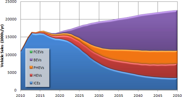
FIGURE H.12 Vehicle sales by vehicle technology assuming optimistic PEV technology estimates.
_____________________________
11 Although it is assumed that, all else equal, BEVs will be driven two-thirds as much as ICEs, usage is also affected by vehicle age and energy costs per kilometer.
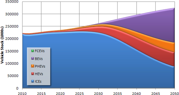
FIGURE H.13 Vehicle stock by vehicle technology assuming optimistic PEV technology estimates.
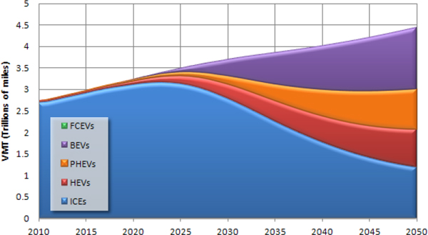
FIGURE H.14 Vehicle miles traveled by vehicle technology assuming optimistic PEV technology estimates.
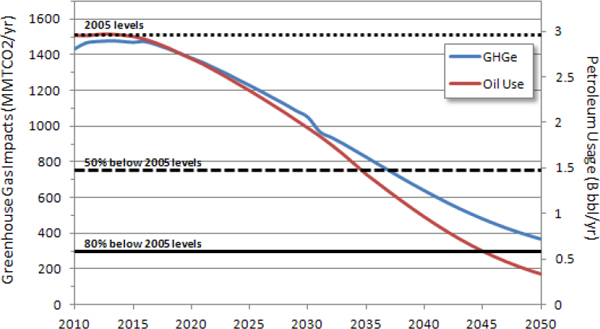
FIGURE H.15 Changes in petroleum use and GHG emissions compared to 2005 assuming optimistic PEV technology estimates and a low-GHG electric grid.
H.4.2 Hydrogen Fuel Cell Vehicles
Using the optimistic projections of FCEV technology and the midrange assumptions for all others makes it easier to introduce FCEVs (lower implicit subsidies) and increases their ultimate, sustainable market share to 75 percent. Total implied subsidies begin at $17,500 per vehicle in 2015 but can be decreased immediately thereafter. Transition subsidies can be eliminated by 2022, leaving social cost feebates in place. Sales of FCEVs are 12,000 in 2015, 22,000 in 2016 and 33,000 in 2017. In 2025, sales exceed 4 million units (Figure H.16). This transition exceeds the speed limit for transitions, with 10.0 percent of the market converting to FCEVs in 2026.
Assuming the low-carbon production of hydrogen but not advanced biofuels, this case appears to be able to meet all goals. Due to the rapid introduction of FCEVs and the substantial increase in energy efficiencies of all vehicles, petroleum use in 2030 is 50 percent lower than it was in 2005. By 2050, petroleum use by LDVs has been eliminated (replaced by 13.5 billion GGE of thermochemical biofuel and 7 billion gge of corn ethanol). GHG emissions are down 90 percent (Figure H.17).
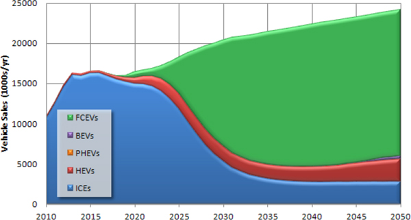
FIGURE H.16 Vehicle sales by vehicle technology assuming optimistic fuel cell electric vehicle (FCEV) technology estimates and policies that promote FCEV use.
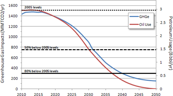
FIGURE H.17 Changes in petroleum use and GHG emissions compared to 2005 assuming optimistic FCEV technology estimates and policies that promote FCEV use.
H.5 REFERENCES
EIA (Energy Information Administration). 2011. Annual Energy Outlook 2011. DOE/EIA-0383(2011). Wasington, D.C.: Department of Energy, Energy Information Administration. March.
Greene, D.L. 2001. TAFV Alternative Fuels and Vehicles Choice Model Documentation. ORNL/TM-2001/134. Oak Ridge, Tenn.: Oak Ridge National Laboratory. July.
———. 2010. How Consumers Value Fuel Economy: A Literature Review. EPA-420-R-10-008. Washington, D.C.: U.S. Environmental Protection Agency. March.
———. 2011. Uncertainty, loss aversion, and markets for energy efficiency. Energy Economics 33:608-616.
———. 2012. Rebound 2007: Analysis of U.S. light-duty vehicle travel statistics. Energy Policy 41:14-28.
Greene, D.L., P.N. Leiby, B. James, J. Perez, M. Melendez, A. Milbrandt, S. Unnasch, and M. Hooks. 2008. Analysis of the Transition to Hydrogen Fuel Cell Vehicles & the Potential Hydrogen Energy Infrastructure Requirements (S. McQueen, ed.). ORNL/TM-2008/30. Oak Ridge, Tenn.: Oak Ridge National Laboratory.
Hamilton, J.D. 2009. Understanding crude oil prices. The Energy Journal 30(2):179-206.
Interagency Working Group on Social Cost of Carbon. 2010. Technical Support Document: Social Cost of Carbon for Regulatory Impact Analysis Under Executive Order 12866, February, 2010. U.S. Government. Available at http://www.epa.gov/otaq/climate/regulations/scc-tsd.pdf.
Lin, Z., and D.L. Greene. 2011a. Promoting the market for plug-in hybrid and battery electric vehicles: The role of recharge availability. Transportation Research Record, in press.
———. 2011b. Significance of daily VMT variation over time and among drivers on assessment of PHEV energy impact. Transportation Research Record, in press.
Melaina, M.W. 2009. Discrete Choice Analysis of Consumer Preferences for Refueling Availability. FY 2009 Annual Progress Report to the DOE Hydrogen Program. Available at http://www.hydrogen.energy.gov/pdfs/progress09/vii_5_melaina.pdf.
Melaina, M.W. and J. Bremson. 2008. Refueling availability for alternative fuel vehicle markets: Sufficient urban station coverage. Energy Policy 36(8):3223-3231.
NHTSA (National Highway Traffic Safety Administration). 2006. Vehicle Survivability and Travel Mileage Schedules. DOT HS 809 952. Washington, D.C.: U.S. Department of Transportation. January.
Nicholas, M., and J.M. Ogden, 2007. Detailed analysis of urban station siting for California hydrogen highway network. Transportation Research Record 1983, pp. 121-128.
Nicholas, M.A., S.L. Handy, and D. Sperling. 2004. “Siting and Network Analysis Methods for Hydrogen Stations Using Geographical Information Systems,” 83rd Annual Meetings of the Transportation Research Board, January 11-15, Washington, D.C.
NRC (National Research Council). 2008. Transitions to Alternative Transportation Technologies: A Focus on Hydrogen. The National Academies Press, Washington, D.C.
———. 2010. Transitions to Alternative Transportation Technologies: Plug-in Hybrid Electric Vehicles. The National Academies Press, Washington, D.C.
Ogden, J.M., and M. Nicholas. 2010. Analysis of a ‘cluster’ strategy for introducing hydrogen vehicles in Southern California. Energy Policy 39(4):1923-1938.
Singh, M., A. Vyas, and E. Steiner. 2003. VISION Model: Description of Model Used to Estimate the Impact of Highway Vehicle Technologies and Fuels on Energy Use and Carbon Emissions to 2050. Prepared by Argonne National Laboratory, Argonne, IL, for the Department of Energy under Contract No. W-31-109-ENG-38. Report#ANL-ESD-04-1. December.
Small, K.A., and H.S. Rosen. 1981. Applied welfare economics with discrete choice models. Econometrica 49(1):105-130. January.
Ward, J. 2008. VISION 2008 User’s Guide. Prepared by the U.S. Department of Energy, Energy Efficiency and Renewable Energy, Vehicle Technologies Program. Report #ANL-08/34. October. Available at http://www.transportation.anl.gov/pdfs/TA/534.pdf.


