
5
Modeling the Transition to Alternative Vehicles and Fuels
Achieving the goals of reducing light-duty vehicle (LDV) petroleum use and greenhouse gas (GHG) emissions by 80 percent by 2050 and petroleum use by 50 percent by 2030 is likely to require a transition from internal combustion engines powered by fossil petroleum to alternative fuels or vehicles or both. There is also potential for significant technological advancement both in the LDV fleet and in the fuel and fueling infrastructure that will power vehicles over the next 40 years. Which of these technologies will actually enter the market depends on a range of factors, including the extent of progress in the different vehicle and fuel technologies, market conditions in gasoline and other fuels markets that will affect cost and competiveness, consumer preferences over vehicle and fuel characteristics, and government policies toward this sector. Government policies are likely to be particularly important because the benefits of both petroleum and greenhouse gas reductions accrue to the public as a whole, and so market forces alone cannot be relied on to provide sufficient reductions.1
Two different models were used by the committee to assess the potential and opportunities for achieving the goals of this study. The first was the VISION model developed by Argonne National Laboratory (Singh et al., 2003). This spreadsheet model was an ideal starting point for the committee’s analysis because it has been widely used in the past for light-duty vehicle (LDV) sector forecasts of energy use and GHG emissions. All inputs must be specified, including future rates of penetration of vehicle and fuel types and the costs of each. VISION does not, however, attempt to estimate how markets will react to alternative vehicles and fuels or to the policies that may be needed to successfully introduce them.
The second model, the Light-duty Alternative Vehicle Energy Transitions (LAVE-Trans) model, incorporates market decision making and reflects the most significant economic barriers to the adoption of new vehicles and fuels. It therefore allows for assessment of policies and possible transition paths to attain the goals. Penetration rates of different vehicle and fuel types are determined in this model in response to price, costs, and vehicle fueling characteristics; they are not simply assumed as they are in VISION. Moreover, LAVE-Trans includes a consistent and comprehensive assessment of the benefits and costs of different policy and technology pathways over time.
It is important to emphasize the nature and extent of the uncertainties that lie behind all of the analyses in this chapter. First, the analysis uses estimated improvements to fuel efficiency and fuel carbon content, and the associated costs, for vehicles up to the 2050 model year as provided by expert members of this committee, evidence from the literature, and consultation with experts outside the committee. (Detailed descriptions can be found in Chapters 2 and 3.) Both models use the same GHG emissions, fuel economy, and vehicle cost estimates. These estimates by necessity reflect numerous assumptions, most of which are highly uncertain, particularly when such forecasts are made far into the future. One way the committee represents this uncertainty is to include both “midrange” and “optimistic” estimates for important variables such as vehicle fuel efficiency and fuel carbon intensities. However, it is difficult to reflect the full range of uncertainty. Thus, a “pessimistic” case is not included here for vehicles in which either technology does not progress very rapidly or costs do not come down over time and with volume as expected.
There is, in addition, uncertainty in the assumptions about consumer preferences for different vehicle characteristics,
_______________________
1Both petroleum use reduction and GHG emissions reduction are types of public goods in that once they are reduced, all members of society benefit through greater security and reduced risk of global climate change. No one is excluded from these benefits. The private sector will tend to underprovide such goods because private individuals must pay the costs of reductions but do not get all of the benefits—the benefits are shared by all. When there are public goods, then, government action may be essential for attaining amounts of the public goods that are economically efficient for society (Boardman et al., 2011).
including range and limited fuel availability for alternatives such as hydrogen fuel cell vehicles.2 A sensitivity analysis illustrating uncertainties about the market’s response to alternative vehicles and fuels is described in Section 5.7. There is also controversy about the magnitude of the social cost of GHG emissions and the social cost of the United States’ reliance on oil and petroleum-based gasoline. The estimates used in this report are drawn from the most recent literature but do not reflect the full range of uncertainty. Finally, it is extremely difficult to model all of the feedback effects that will inevitably result over time as technology development and markets interact.
Despite the inherent uncertainties in attempting to forecast four decades into the future, the committee’s modeling effort here uses the best available evidence and information and makes plausible assumptions where sound data are missing. Analysis of the results from the two models then provides useful insights about what various vehicles and fuel combinations can achieve, the nature of the processes by which changes will occur, and the general magnitude of potential costs and benefits of different policy options.
5.2 MODELING APPROACH AND TOOLS
VISION is designed to extend the transportation sector-specific component of the National Energy Modeling System (NEMS) used by the Energy Information Administration (EIA). It provides longer-term forecasts of energy use and GHG emissions than does NEMS. While not as detailed or comprehensive as the NEMS model, VISION provides greater flexibility to analyze a series of projected usage scenarios over a much longer timeframe. It has been used extensively in the literature.
For the purposes of this study, VISION has been modified in a number of ways. The most up-to-date assumptions from the committee about vehicle efficiencies, fuel availability, and the GHG emissions impacts of using those fuels have been included. It is assumed that new-technology vehicle sales ramp up slowly and that new sales for a particular vehicle type never increase by more than about 5 percent of total new LDV sales in a given year. In addition, only one plug-in hybrid electric vehicle (PHEV), a PHEV-30 with a real-world all-electric driving range of 25 miles, is included. It is assumed that because of their limited range, battery electric vehicles are to be driven 1/3 fewer miles per year than other vehicles (Vyas et al., 2009) and that any decrease in miles driven by electric vehicles will be offset by increased mileage from other vehicles. Total new car sales and annual vehicle miles traveled (VMT) are assumed to be the same as in the projections from the Annual Energy Outlook 2011 (AEO; EIA, 2011a), and there is no assumption of a “rebound effect”3 if the cost of driving a mile declines. Adjustments to VMT can be included separately in any VISION run assessment.4 Finally, GHG estimates from biofuels include both emissions from production and from indirect land-use changes (see Chapter 3).
The committee uses the VISION model to explore how a focus on specific technologies or alternative vehicle and fuel types has the potential to reduce oil use and GHG emissions to achieve the study goals. The committee then turns to the LAVE-Trans model to shed light on how policies might be used to achieve the needed transitions.
The Light-duty Alternative Vehicle Energy Transitions (LAVE-Trans) model uses a nested, multinomial logit model5 of consumer demand to predict changes in the efficiency of vehicles and fuels over time, including a possible transition to alternatively fueled vehicles. Any transition to these advanced vehicles faces a number of barriers, including high costs due to the lack of scale economies and lack of learning, consumer uncertainty about safety or performance, and the lack of an energy supply infrastructure. Each of these barriers has been incorporated into the LAVE-Trans model so that the costs of overcoming them and, alternatively, the benefits of policies needed to do so can be measured (subject to the limits of current knowledge).
The model incorporates an array of factors that affect and are derived from consumer behavior, including the rebound effect; “range anxiety” and perceived loss of utility, particularly as it pertains to the availability of a fueling infrastructure; aversion to new technology and its reciprocal effect, early adoption; and the significant discounting of future fuel benefits over the lifetime of the vehicle. Nine variables influence the market shares of the alternative advanced technologies:
_______________________
2Thanks to recent research, such issues are better understood than they were a decade ago (e.g., UCD, 2011; Bastani et al., 2012), yet much remains to be learned.
3Improvements in the efficiency of energy consumption will result in an effective reduction in the price of energy services, leading to an increase of consumption that partially offsets the impact of the efficiency gain in fuel use. This is known as the “rebound effect.”
4If a 5 percent reduction in vehicle miles traveled is plausible under certain policies, then the estimates of GHG emissions and oil use can be reduced by 5 percent.
5A multinomial logit model is a standard model often used to represent consumer choice where there is a finite set of discrete options. The probability of choosing among the set of available options is governed by representative parameters for a particular class of consumer. A nested model refers to multiple layers of choice (see Daly and Zachary, 1979; McFadden, 1978; Williams, 1977). For example, the first level of choice in the LAVE-Trans model is between choosing whether or not to buy an LDV. If a consumer chooses to buy an LDV, the next level of choice is between purchasing a passenger car or a light truck. Then, within a particular class of vehicle there are multiple options, such as whether to purchase an ICEV, FCEV, or BEV. Further description of the LAVE-Trans nested multinominal logit model can be found in Section H.2 in Appendix H.
- Retail price equivalent (RPE),
- Energy cost per kilometer,
- Range (kilometers between refuel/recharge events),
- Maintenance cost (annual),
- Fuel availability,
- Range limitation for battery electric vehicles (BEVs),
- Public recharging availability,
- Risk aversion (innovator versus majority), and
- Diversity of make and model options available.
It also includes policy options that affect consumer choices, including new-vehicle rebates, incentivized infrastructure development, and fuel-specific taxation. Although both the LAVE-Trans and VISION models use the same committee-developed technology and cost assumption for different vehicles and fuels over time, the LAVE-Trans model represents a significant improvement over the VISION model in several ways. First, because it includes consumer behavior in the vehicle market, it is able to predict the shares of different vehicles that enter the market in response to policy and market changes, whereas VISION must assume these shares over time. Thus, LAVE-Trans is much better able to assess the types of policies that may be necessary to achieve the goals addressed in the present study. Second, LAVE-Trans can be used to assess the full range of benefits and costs of different policies. The committee’s approach to measuring benefits and costs is discussed more fully below.
5.3 RESULTS FROM RUNS OF VISION MODEL
Forecasts of the penetration rates of different types of vehicles using the VISION model must be compared to some alternative outcome in which there are no further policy actions and limited technological advances. In this analysis, two such cases are presented. One is the business as usual (BAU) case. It closely follows the AEO 2011 reference case projection to 2035 and from there is extrapolated to 2050. In this case, NHTSA CAFE and EPA GHG emission joint standards for LDVs are set out to 2016, with fuel economy continuing to increase to 2020 per the Energy Independence and Security Act of 2007. Renewable fuel production increases in response to RFS2 (the amended Renewable Fuel Standard), but it is assumed that financial and technological hurdles facing advanced biofuel projects will delay compliance. The other case is the Committee Reference Case. It adds to the BAU case the CAFE rules that have been set through the 2025 model year, and the levels of advanced biofuels production required under RFS2 are assumed to be fully met by 2030 through the production of thermochemical cellulosic biofuel.
5.3.1.1 Business as Usual (BAU)
In the BAU case, new-vehicle sales increase to 22.2 million in 2050 from 10.8 million units in 2010 (a year in which sales were severely depressed due to the recession). Diesel, hybrid, and plug-in hybrid vehicles make modest gains in market share (Figure 5.1). The total stock of LDVs increases from about 220 million in 2010 to 365 million in 2050.
Fleet average on-road fuel economy improves from 20.9 miles per gallon gasoline equivalent (mpgge; equivalent to a consumption of 4.8 gge/100 mi) in 2005 to 34.7 mpgge (or 2.9 gge/100 mi) in 2050. This is consistent with the Energy Independence and Security Act of 2007, which requires a fleetwide fuel economy test value of at least 35.5 mpg in 2020 and includes modest improvements in vehicle efficiency thereafter. This is enough to offset most of the forecasted increase in vehicle travel from 2.7 trillion to 5.0 trillion miles. Energy use increases to 159 billion gallons gasoline equivalent (billion gge) from 130 billion gge. Com-
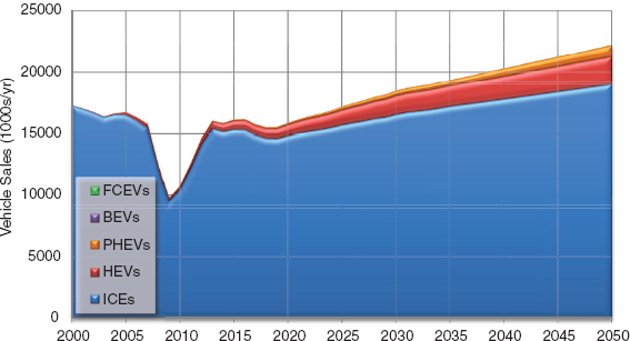
FIGURE 5.1 Vehicle sales by vehicle technology for the business as usual scenario.
pared to 2005 levels, petroleum use remains unchanged, the result of increased use of corn-based ethanol (to 12.0 billion gge/yr in 2050) and the addition of 8.9 billion gge/yr of cellulosic ethanol and 8.1 billion gallons of gasoline produced from coal. The net effect of increased overall energy use and the shift to a somewhat less carbon-intensive fuel mix is a 12 percent increase in 2050 GHG emissions.
Oil prices in this scenario are expected to gradually increase to $123/bbl by 2035 (in 2009$) according to AEO 2011, resulting in a pre-tax gasoline price of $3.16 in 2035. Gasoline prices are then extrapolated out to 2050 assuming the compound rate of growth modeled in AEO 2011 from 2030 to 2035, yielding a pre-tax price of $3.37. The current gasoline tax of $0.42/gal is assumed to remain the same (in constant dollars) out to 2050. Gasoline prices in this scenario are shown in Figure 5.2. The pre-tax fraction of these gasoline prices is assumed in all modeling scenarios.
5.3.1.2 Committee Reference Case
The committee further defined its own reference case to include all of the midrange assumptions it developed about vehicle efficiencies, fuel availability, and GHG emission rates up to 2025 (summarized in Chapters 2 and 3). This Committee Reference Case assumes that the 2025 fuel efficiency and emissions standards for LDVs will be met. The committee interprets the standards to require that new vehicles in 2025 must have on-road fuel economy averaging around 40 mpg (given a fleetwide CAFE rating of 49.6 mpg for new vehicles, the difference between on-road and test values, and the likely application of various credits under the CAFE program). See Box 5.1 for an explanation of on-road fuel economy compared to tested fuel economy ratings.
This case also assumes that the RFS2 goals will be met by 2030. As a result, corn ethanol sales rise to almost 10 billion gge/yr by 2015 and then remain at that level. Based on the analysis in Chapter 3, it is also assumed that all cellulosic biofuels will be thermochemically derived gasoline. The RFS2 requirements result in annual production of 13.2 billion gallons of such biofuels by 2030 and roughly constant levels thereafter.
Under the assumptions of the Committee Reference Case, the fuel economy (fuel consumption) of the stock of LDVs in use improves to 35.5 mpgge (2.8 gge/100 mi) in 2030 and to 41.6 mpgge (2.4 gge/100 mi) in 2050, up from 20.8 mpgge (4.8 gge/100 mi) in 2005 (Figure 5.3). This improvement is largely due to efficiency improvements in internal combustion engine vehicles (ICEVs) as well as increasing sales of hybrid electric vehicles (HEVs). Hybrids are more successful in this scenario compared to the BAU case, increasing their share of new-vehicle sales to 33 percent (7.3 million units) by 2050.
Greenhouse gas emissions are 30 percent below 2005 levels in 2030, at 1,057 million metric tons CO2 equivalent (MMTCO2e) per year, but rise again and are just 22 percent below in 2050 (1,121 MMTCO2e/yr) as VMT continues to rise while the efficiency of the on-road fleet remains approximately constant (Figure 5.4). Petroleum use is 36 percent below the 2005 level in 2030 (1.91 billion bbl/yr) and 30 percent below in 2050 (2.09 billion bbl/yr), also rising with
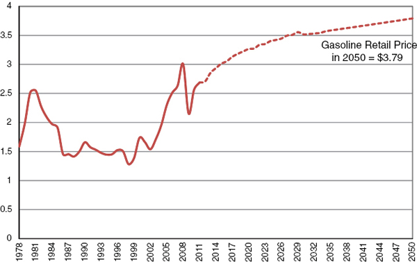
FIGURE 5.2 Retail gasoline fuel prices (1978-2050), including federal and state taxes. Projected values shown as dotted line. SOURCE: Data from Annual Energy Review 2010 [1978-2010] (EIA, 2011b), Annual Energy Outlook 2011 [2010-2035] (EIA, 2011a), and extrapolation by the committee using the compound annual growth rate for 2030-2035 (0.42%) [2035-2050].
BOX 5.1
The Distinction Between “As Tested” and “Actual In-Use” Fuel Consumption
A large difference exists between the fuel economy (miles per gallon, or mpg) figures used to certify compliance with fuel economy standards and those experienced by consumers who drive the vehicles on the road and purchase fuel for their vehicles. The numbers used to certify compliance with the Corporate Average Fuel Economy (CAFE) standards are based on two dynamometer tests. These test values are also the numbers discussed and presented in the tables and figures of this report. A different 5-cycle test procedure is used to compute the Environmental Protection Agency (EPA) “window-sticker” (label) fuel economy ratings that are used in automotive advertising, most car-buying guides, and car-shopping Websites. Neither procedure accurately reflects what any given individual will achieve in real-world driving. Motorists have different driving styles, experience different traffic conditions, and take trips of different lengths and frequencies. Realized fuel economy also varies with factors including climate, road surface conditions, hills, temperature, tire pressure, and wind resistance. The impacts of air conditioning, lighting, and other accessories on fuel consumption are not included in the two-cycle tests.
Both CAFE mpg and “window-sticker” mpg were based on the values determined via standardized city- and highway-cycle procedures that were codified by law in 1975. The divergence between test-cycle values and real-world experience was recognized and in 1985 the EPA revised calculation procedures for the window-sticker ratings in order to bring them more in line with the average performance motorists were reporting in real-world driving. From 1985 through 2007, the window sticker values averaged about 15 percent lower than the unadjusted values used for CAFE regulation. The label values were updated starting in model year 2008, and the update further increased the difference between CAFE and “window sticker” values by factoring in additional adjustments, so that the current window sticker values average about 20 percent lower than those used for regulation.
The results can be confusing. For example, the 2017-2025 CAFE rules envision a 49.6-mpg “fleet average new LDV fleet fuel economy” for the 2025 model year, but acknowledge that real-world fuel economy will be significantly lower—probably somewhere below 40 mpg. A further complication is that the “National Plan” (the joint rulemaking by NHTSA and EPA) regulates greenhouse gas (GHG) emissions in addition to fuel economy. Because some technologies for reducing LDV GHG emissions do not involve fuel economy, EPA now also reports a “mpg-equivalent” value representing the CAFE fuel economy that would be needed to achieve a similar degree of GHG emissions reduction. That type of number is the one given as the 54.5 mpg “equivalent” stated in many discussion of the 2025 target; it reflects special credits for various technologies that can help in achieving fleet average GHG emissions of 163 grams per mile by 2025.
The CAFE numbers represent a higher fuel economy than most consumers are likely to experience on the road. The estimates of actual fuel consumption and associated GHG emissions presented in this report, however, reflect a downward fuel economy adjustment for approximating real-world impacts. Although there is no universally agreed-upon method for converting test values to on-road values, the committee has determined that an appropriate estimate for analytic purposes can be obtained by adjusting the CAFE values downward by about 17 percent (i.e., multiplying by 0.833). That factor is used whenever the report discusses “average” on-road values.
VMT. Thus, the Committee Reference Case, which assumes current policies included in the AEO BAU case augmented by the proposed 2025 fuel economy and emissions standards and RFS2 compliance, does not come close to meeting the 2030 or 2050 goals.
To explore possible paths to attain the goals addressed in this study, VISION was run for a range of cases. The predominant characteristic of these runs is to focus on a market dominated by a particular vehicle type and alternative fuel (e.g., electric vehicles and grid with reduced GHG emissions, or fuel cell vehicles and hydrogen generated with CCS). To assess the range of possibilities, the committee looked at runs that used the midrange vehicle efficiencies as well as at runs that used the optimistic efficiencies representing technological progress proceeding more rapidly than expected, as described in Chapter 2. From the fuels side, the committee considered both present methods of producing a fuel as well as fuel supply technologies with reduced GHG impacts as described in Chapter 3. Each of the possible fuel types is shown in Table 5.1. A brief description below of each of the scenarios modeled with VISION identifies the important assumptions and variation in those assumptions. Section H.1 in Appendix H provides further detail.
- Emphasis on ICEV efficiency. These runs continue the reference case’s focus on LDV fuel efficiency improvements through the period to 2050. Shares of advanced ICEVs and HEVs increase to about 90 percent of new-vehicle sales by 2050. Two runs are included that differ only in their assumptions about the fuel efficiency improvements of vehicles over time. The first assumes the midrange assumptions for fuel efficiency for all technologies (Chapter 2, Table 2.12), and the second assumes optimistic fuel efficiency for ICEs and HEVs while maintaining midrange values for the small numbers of other types of vehicles in the fleet. It is assumed that the RFS2
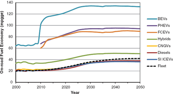
FIGURE 5.3 Average on-road fuel economy for the Reference case light-duty vehicle stock. In most cases, the average efficiency plateaus as the fleet gradually turns over to vehicles that meet the 2025 model year CAFE standard. There are small reductions over time with rising use of advanced technologies in trucks.
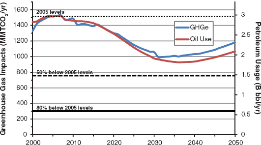
FIGURE 5.4 Petroleum use and greenhouse gas emissions for the Committee Reference Case.
requirements described in the Committee Reference Case, above, are still in place. These increased vehicle efficiency cases require much less liquid fuel over time and assume that gasoline is the fuel reduced.
- Emphasis on ICEV efficiency and biofuels. These two runs are similar to the case described above. The difference is that more biofuels are brought into the market after 2030, as described in Table 5.1. The modeling runs assume this additional biofuel, largely in the form of drop-in gasoline that displaces petroleum, and the only difference in the two runs is the assumption of vehicle fuel efficiency. The first run assumes all vehicles are at the midrange efficiency, and in it the share of petroleum-based gasoline as a liquid fuel falls to about 25 percent by 2050. The second run assumes optimistic fuel efficiency for ICEVs and HEVs. In this case, bio-based ethanol, bio-based gasoline, and a small amount of coal-to-liquid (CTL) and gas-to-liquid (GTL) fuels make up all liquid fuel, with almost no petroleum-based gasoline.
- Emphasis on fuel cell vehicles. This case comprises 4 different runs of VISION, to capture variation in both vehicle efficiency and fuel carbon content. In all of these runs, the share of fuel cell electric vehicles (FCEVs) increases to about 25 percent of new car sales by 2030 and then to 80 percent by 2050, modeled on the maximum practical deployment scenario from Transition to Alternative Transportation
TABLE 5.1 Description of Fuel Availabilities Considered in Modeling Light-Duty Vehicle Technology-Specific Scenarios
| Fuel Type | Description (values reflect annual production in 2050) |
| AEO 2011 | AEO 2011 projection extrapolated to 2050; 12.0 billion gge corn ethanol; 8.9 billion gge cellulosic ethanol; 8.1 billion gal CTL gasoline |
| Reference | RFS2 met by 2030: 10 billion gge corn ethanol; up to 13.2 billion gge cellulosic thermochemical gasoline; up to 3.1 billion gge CTL; up to 4.6 billion gge GTL |
| Biofuels | Includes Reference biofuel availability plus additional drop-in biofuels: Up to 45 billion gge cellulosic thermochemical gasoline; 10 billion gge corn ethanol |
| AEO 2011 | AEO 2011 Electricity Grid: 541 g CO2e/kWh; |
| Electricity Grid | 46% coal, 22% natural gas, 17% nuclear, and 12% renewable |
| Low-C | AEO 2011 Carbon Price Grid: 111 g CO2e/kWh; 6% |
| Electricity Grid | coal, 25% natural gas, 12% natural gas w/CCS, 30% nuclear, and 23% renewable |
| Low-Cost H2 | Lowest Cost: $3.85/gge H2; 12.2 kg CO2e/gge H2; |
| Production | 25% distributed natural-gas reforming, 25% coal gasification, 25% central natural-gas reforming, and 25% biomass gasification |
| CCS H2 | Added CSS: $4.10/gge H2; 5.1 kg CO2e/gge H2; 25% |
| Production | distributed natural-gas reforming, 25% coal gasification w/CCS, 25% central natural-gas reforming with CCS, and 25% biomass gasification |
| Low-C H2 | Low CO2 emissions: $4.50/gge H2; 2.6 kg CO2e/ |
| Production | gge H2; 10% distributed natural-gas reforming, 40% central natural-gas reforming w/CCS, 30% biomass gasification, and 20% electrolysis from clean electricity |
NOTE: CCS H2 case analyzed by LAVE model, not VISION.
Technologies: A Focus on Hydrogen (NRC, 2008). There are two runs with the midrange vehicle fuel efficiencies, the first with low-cost hydrogen production (Low-Cost H2 Production) and the second with low-GHG hydrogen production (Low-C H2 Production), described in Table 5.1. Finally, there are two additional runs with optimistic assumptions about the fuel efficiency of FCEVs, each with the different assumptions for the GHG emissions from hydrogen production.
- Emphasis on plug-in electric vehicles. There are 4 VISION runs emphasizing plug-in electric vehicles (PEVs) to account for differences in assumptions about vehicle efficiency as well as GHG emissions impacts of the fuel. In all runs, the share of BEVs and PHEVs increases to about 35 percent of new LDV sales by 2030 and 80 percent by 2050, in line with the rates put forth in Transitions to Alternative Transportation Technologies: Plug-In Hybrid Electric Vehicles (NRC, 2010a). Relatively greater sales of PHEVs than BEVs in all years are assumed (see Table H.3 in Appendix H for details). Each of the two runs in each pair of runs—midrange and optimistic—uses a different assumption about GHG emissions from the electricity grid (AEO 2011 Grid and Low-C Electric Grid, Table 5.1). The low-emissions grid is assumed to emit 25 percent of GHGs per unit of generation compared to the BAU grid by 2050.
- Emphasis on natural gas vehicles. These runs assume that sales of compressed natural gas vehicles (CNGVs) are 25 percent of the market by 2030 and 80 percent by 2050. In both midrange and optimistic cases, CNG fuel use rises over time, and so little liquid fuel is needed by 2050 that it is assumed that no CTL and GTL plants are ever built. It is further assumed that RFS2 must be met by 2030, and so the liquid fuel that is used is primarily biofuels in both of these runs.
5.3.3 Results of Initial VISION Runs
Figures 5.5 to 5.7 indicate the results of the VISION model runs described above. The total amount of each type of fuel used in each scenario is shown in terms of energy use (billions of gallons of gasoline-equivalent). For the hydrogen and electricity cases, the fuels are not broken down by carbon content. Figure 5.5 shows results of the assumptions about fuel use that were made for the different VISION runs. For example, the total amount of liquid fuels used is the same for the Efficiency and Efficiency + Biofuels scenarios—it is assumed that it is the fraction of that fuel generated from biomass that is different. Higher prices for biofuels are likely to drive liquid fuel prices up over time and could result in less total liquid fuel used, but that type of market feedback cannot be accounted for in the VISION model runs.
Some ethanol and cellulosic biofuels are used in all of the scenarios because of the assumptions that they will be required under regulations such as RFS2. Over all of the scenarios, fuel energy use is lowest for the Plug-in Electric Vehicle, Hydrogen Fuel Cell Vehicle, and Optimistic Efficiency for ICEV and HEV cases.
Figure 5.6 shows that the long-term petroleum reduction goal of 80 percent by 2050 could occur if there is either (1) a major increase in biofuel availability with high-efficiency ICEVs (including HEVs) or (2) a large increase in alternatively fueled vehicles. All of the cases involving a transition to alternatively fueled vehicles meet or nearly meet a midterm petroleum reduction goal of 50 percent by 2030; in addition, optimistic ICEV efficiencies and widespread availability and use of biofuels could meet this interim goal as well. It is important to note that all of these scenarios assume very aggressive deployment of the specific vehicles and fuels being emphasized. The VISION model cannot address how these vehicle shares would be achieved. The model tells us nothing about how market conditions or policies would produce such results in vehicle and fuel shares.
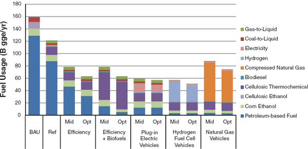
FIGURE 5.5 Fuel usage in 2050 for technology-specific scenarios outlined in Section 5.3.2. Midrange values are the committee’s best estimate of the progress of the vehicle technology if it is pursued vigorously. Optimistic values are still feasible but would require faster progress than seems likely. No GTL or CTL fuel is used in the fuel cell and natural gas scenarios.
Figure 5.7 shows GHG emissions results for each scenario. It is noteworthy that all of the scenarios show substantial emissions reductions from the Committee Reference Case. However, meeting the 80 percent reduction goal is extremely difficult. Even given the aggressive deployment of advanced vehicle technologies and fuel supply technologies 2050 (by Technology) assumed in these runs, only two scenarios meet the 80 percent goal, the FCEV-dominated fleet powered by very low GHG-emitting hydrogen fuel and the optimistic case for vehicle efficiency plus biofuels. Several other scenarios come close to meeting the goal, and small reductions in VMT that could be expected with strict policies to reduce
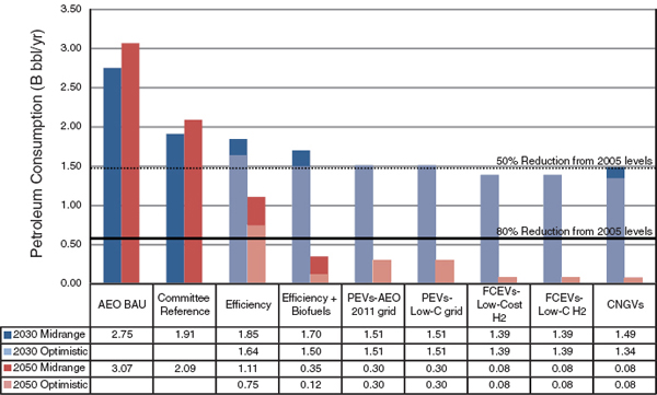
FIGURE 5.6 U.S. light-duty vehicle petroleum consumption in 2030 and 2050 for technology-specific scenarios outlined in Section 5.3.2. Midrange values are the committee’s best estimate of the progress of the vehicle technology if it is pursued vigorously. Optimistic values are still feasible but would require faster progress than seems likely.
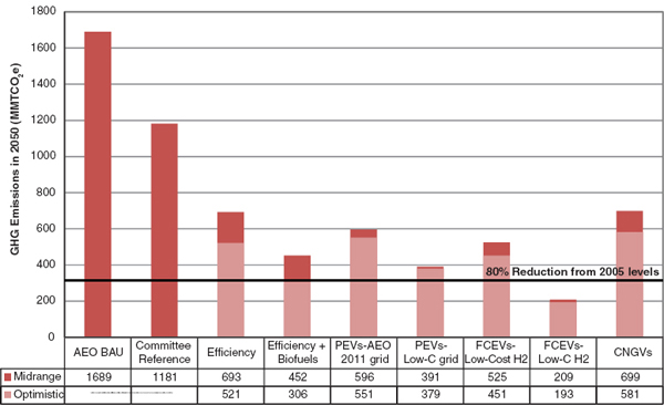
FIGURE 5.7 U.S. light-duty vehicle sector greenhouse gas emissions in 2050 for technology-specific scenarios outlined in Section 5.3.2. Midrange values are the committee’s best estimate of the progress of the vehicle technology if it is pursued vigorously. Optimistic values are still feasible but would require faster progress than seems likely.
GHGs might be sufficient to push them to the 80 percent goal as well.
Although these model results illustrate penetration levels of certain vehicles and fuels that may achieve the petroleum usage and/or greenhouse gas emissions reductions desired, the VISION model does not estimate the cost or the policy actions that would be necessary. For this, an alternative approach is needed.
The LAVE modeling builds on the VISION analyses, illustrating how market responses may influence the task of achieving the petroleum and greenhouse gas reduction goals as well as providing a sense of the intensity of policies that may be required and measuring, very approximately, the costs and benefits. The committee recognizes that such estimates will be neither certain nor precise. Both market and technological uncertainty are very substantial, as is illustrated in Section 5.7, a fact that requires an adaptable policy process. However, ignoring market responses and the costs of necessary policies would be a mistake. The policy options included in the LAVE model are briefly summarized in Box 5.2 and described in greater detail in Section 5.4.2.
The analyses using the LAVE-Trans model proceed as follows. First, the LAVE-Trans and VISION model projections of the BAU case are compared to establish the general consistency of the two models. The LAVE-Trans model is then used to approximately replicate the VISION model scenarios, which again shows broad consistency but also some differences between the two models. The strategy and approach to policy analysis using the LAVE-Trans model are described next, including how costs and benefits have been measured. All of the policy scenarios described below include strict CAFE standards that are tightened over time, and also some policy approach to bring alternative fuels into the market, such as RFS2. In addition all policy scenarios below also include the Indexed Highway User Fee (IHUF).
- The first set of policy analyses explore what might be achievable by means of continued improvement of energy efficiency beyond 2025 and introduction of large quantities of “drop-in” biofuels with reduced greenhouse gas impacts produced by thermochemical processes. To provide incentives for greater efficiency from ICEs and HEVs, the first feebate policy in Box 5.2, the Feebate Based on Social Cost (FBSC) is introduced.
- A second set explores the potential impacts of policies that change the prices of vehicles and fuels to reflect the goals of reducing GHG emissions and petroleum use. In these model runs, stronger feebates
BOX 5.2
Policies Considered in the LAVE-Trans Model
Feebates Based on Social Cost (FBSC)—An approximately revenue neutral feebate system that precisely reflects the assumed societal willingness to pay to reduce oil use and GHG emissions (see Boxes 5.3, 5.4, and 5.5 on feebates and the values of GHG and oil reduction).
Indexed Highway User Fee (IHUF)—A replacement for motor fuel taxes, the IHUF is a fee on energy indexed to the average energy efficiency of all vehicles on the road and is designed to preserve the current level of revenue for the Highway Trust Fund (see Chapter 6 for details).
Carbon/Oil Tax—A gradually rising tax levied on fuels to reflect the societal values of their carbon emissions and petroleum content (see Boxes 5.4 and 5.5).
Feebates Based on Fuel Savings—A feebate system that compensates for consumers’ undervaluing of future fuel savings. This feebate reflects the discounted present value of fuel costs (excluding the social cost fuel tax) from years 4 to 15, discounted to present value at 7 percent per year.
Transition Policies (Trans)—Polices that consist of subsidies to vehicles and fuel infrastructure designed to allow alternative technologies to break through the market barriers that “lock in” the incumbent petroleum-based internal combustion engine vehicle-fuel system. These could be either direct government subsidies or subsidies induced by governmental regulations, such as California’s Zero-Emissions Vehicle standards.
on vehicles, those based on fuel savings, are included, and carbon and petroleum taxes are added that reflect estimates of the full social cost of using those fuels.
- The third, fourth, and fifth sets explore transitions from ICEVs fueled by petroleum to plug-in electric vehicles, fuel cell vehicles powered by hydrogen, and compressed natural gas vehicles, respectively. These all include transition policies tailored to the particular vehicle and fuel type being considered.
- Two final groups of cases consider combinations of PEVs and FCEVs and the implications of more optimistic technological progress. These also include the appropriate transition policies.
- Finally, the implications of uncertainty about technological progress and the market’s response to advanced technologies and transition policies are considered. These cases include the IHUF, FBSC feebate, and transition policies while examining varied assumptions of technological progress and market behavior.
5.4.1 Comparing LAVE-Trans and VISION Estimates
As shown in Table 5.2, the BAU cases from the LAVE-Trans and VISION models confirm the general consistency of the two models. Each was calibrated to match in all years with respect to total vehicle miles of travel and total vehicle sales. There are differences in new-vehicle and vehicle stock fuel economies, the distributions of stock by age, and in the starting year GHG emissions rates due to the use of two different starting base years.6 These lead to differences between the models of about 5 percent in energy and GHG emissions estimates in 2010, with the differences declining in subsequent years. This decline reflects the fact that the differences are chiefly due to the starting-year data for vehicle stocks and LDV energy efficiency and usage.
LAVE-Trans models vehicle purchase decisions and vehicle use in ways that VISION does not, enabling it to include market responses to improvements in vehicle technologies. If vehicles have fuel economy gains that are more than paid for by their fuel savings, for example, consumers will purchase more vehicles and the size of the vehicle stock will increase. If vehicle efficiency improves but fuel prices do not increase proportionately, vehicle use will increase. Market shares of vehicle technologies are not assumed in LAVE-Trans as they are in VISION but are based on a model of consumer choice that accounts for the prices, energy costs, and other attributes of the different technologies. All of these factors change a great deal over time in all cases.
The purchase prices and energy efficiencies of future vehicles strongly affect their market acceptance. In the LAVE-Trans model, novel technologies start out at a significant disadvantage relative to ICEV and HEVs because millions of these latter vehicles have already been produced and can access a ubiquitous infrastructure of refueling stations. Novel technologies must progress down learning curves by accumulating production experience and acquire scale economies through high sales volumes. As a result, the initial costs of BEVs, PHEVs, CNGVs, and FCEVs are much higher than the long-run costs projected in the midrange and optimistic scenarios. The long-run costs for passenger cars in Figure 5.8 show what is estimated to be technologically achievable in a given year at fully learned, full-scale production. In the midrange assessment, these potential costs converge between 2030 and 2040, with FCEVs and BEVs becoming slightly less expensive than ICEVs but with PHEVs remaining several thousand dollars more expensive. The optimistic assessment trends are similar but the convergence occurs more rapidly and the advantages of FCEVs and
_______________________
6The LAVE-Trans model has a starting year of 2010, while VISION uses a base year of 2005. Instead of reprogramming or recalibrating the models, it was checked simply that their estimates were consistent.
TABLE 5.2 Comparison of Business as Usual Projections of the VISION and LAVE-Trans Models
| 2010 | 2030 | 2050 | |||||||
| LAVE | VISION | LAVE | VISION | LAVE | VISION | ||||
| Energy use | billion gge | 132 | 126 | 137 | 129 | 158 | 159 | ||
| Petroleum use | billion gge | 124 | 120 | 118 | 115 | 129 | 129 | ||
| Greenhouse gas emissions | MMTCO2e | 1,431 | 1,498 | 1,467 | 1,487 | 1,645 | 1,689 | ||
| Vehicle sales | thousands | 10,797 | 10,797 | 18,502 | 18,502 | 22,219 | 22,219 | ||
| Vehicle stock | thousands | 222,300 | 236,310 | 255,603 | 281,976 | 314,538 | 365,199 | ||
| Vehicle miles traveled | trillion miles | 2.73 | 2.73 | 3.75 | 3.75 | 5.05 | 5.05 | ||
| New light-duty vehicle fuel economy | mpg | 22.5 | 22.6 | 29.8 | 30.3 | 33.8 | 34.8 | ||
| Stock light-duty vehicle fuel economy | mpg | 20.6 | 21.2 | 27.4 | 27.8 | 32.0 | 31.7 | ||
BEVs are greater (see Figures 2.10 and 2.11 as compared with Figures 2.8 and 2.9).
The energy efficiencies of new vehicles are shown in the midrange case to continue to improve at a rapid rate beyond 2025 (see Table 2.12 for details). The new-vehicle fuel economy numbers are inputs to the LAVE-Trans model and are taken from the estimates presented in Chapter 2 after accounting for the difference between on-road and test-cycle values. Internal combustion engine cars (both gasoline and CNG) increase to over 90 mpg by 2050, while HEVs exceed 120 mpg. PHEV fuel economy is the same as HEV mpg when operating in charge-sustaining mode and the same as BEVs when operating in charge-depleting mode. Such large increases in energy efficiency mitigate the effects of fuel prices over time.
The prices of energy are also important and vary substantially among the cases examined below. Figure 5.9 shows the different assumptions about what influences the price of gasoline. The price depends not only on the level at which gasoline is taxed but also on the quantities of biofuel blended into it. Some included cases reflect the use of an IHUF on energy which increases very gradually over time as the average energy efficiency of all vehicles on the road increases. The greatest effect on pump prices, however, is with the introduction of a tax on the social value of carbon emissions and petroleum use, as described in Box 5.3, Box 5.4, and Box 5.5, assumed to be phased in over a period of 5 years. It is important to note that policies that greatly reduce the amount of oil used in the transportation sector, such as a number of those considered here, are likely to reduce both the demand for petroleum and its price. Less domestic use will mean fewer imports from insecure sources, which will likely reduce the magnitude of the social costs of using petroleum.
Figure 5.10 and Figure 5.11 show prices of other fuels under different assumptions. The price of electricity to consumers is affected by the de-carbonization of the grid, the IHUF, and the social value tax. Hydrogen prices start at more than $10/kg at low volumes and decrease as production approaches 6,000 tons/d. When and how quickly the decline occurs varies by scenario according to the level of hydrogen demand.
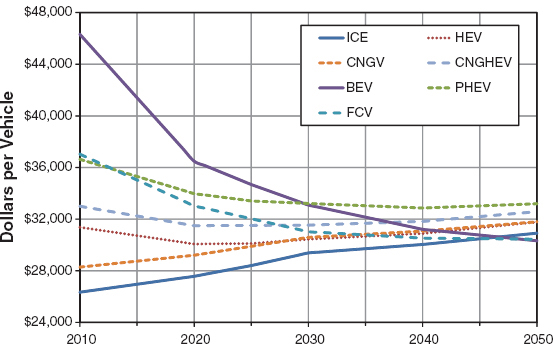
FIGURE 5.8 Fully learned, high-volume retail price equivalents (2009$) assuming midrange technology estimates.
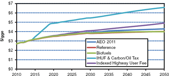
FIGURE 5.9 Retail prices of gasoline (in 2009$) under various policy assumptions.
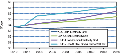
FIGURE 5.10 Retail prices of electricity (in 2009$) under various policy assumptions.
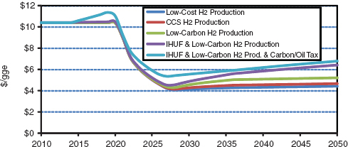
FIGURE 5.11 Retail prices of hydrogen (in 2009$) under various policy assumptions.
BOX 5.3
Feebates
Feebates are a fiscal policy aimed at influencing manufacturers to produce and consumers to purchase vehicles that are more energy efficient or produce fewer GHG emissions or both. A feebate system consists of a metric (e.g., g CO2/mi, gge/mi), a benchmark, and a rate. Each vehicle is compared to the benchmark and is assigned a fee or a rebate according to the difference between its performance on the metric and the benchmark, multiplied by the rate. For example, if the metric is g CO2/mi, the benchmark is 250 and the rate is $20/(g CO2/mi), a vehicle emitting 300 g CO2/mi would pay a fee of $1,000, whereas a vehicle emitting only 150 g CO2/mi would receive a rebate of $2,000. By carefully choosing the benchmark, the feebate system can be made approximately revenue neutral. Benchmarks can be defined in various ways, including as a function of a vehicle attribute, such as the footprint measure (wheelbase × track width) used in the current CAFE standards.
BOX 5.4
The Social Cost of Carbon Emissions
Twelve government agencies conducted a joint study of the social cost of carbon (SCC) to allow agencies to incorporate the social benefits of reducing carbon dioxide emissions into cost-benefit analyses (Interagency Working Group, 2010). The agencies used three well-known economic integrated assessment models (IAMs) to produce the estimates and considered a broad range of factors that affect the damage estimates. Their estimates for the years 2010 to 2050 (Table 5.4.1) represent the present value, in the year in question, of the discounted future damage resulting from a 1 metric ton increase in CO2 emissions. Estimates are given for three different discount rates (5%, 3%, and 2.5%), and for a 95th percentile (5% probability) estimate from the models at a 3 percent discount rate.
The group provided the higher 95th percentile estimate because of the following important limitations of the current state of knowledge concerning future damage due to climate change:
- Incomplete treatment of non-catastrophic damage
- Incomplete treatment of potential catastrophic damage
- Uncertainty in extrapolation of damage to high temperatures
- Incomplete treatment of adaptation and technological changes, and
- Assumption that society is risk neutral with respect to climate damage.
The interagency study strongly recommends using the full range of estimates in assessing the potential damage from climate change (p. 33). The range is an order of magnitude: from $4.70 to $64.90 per metric ton in 2010, rising to $15.70 to $136.20 per metric ton in 2050. In the committee’s judgment, the 80 percent greenhouse gas mitigation goal reflects a societal willingness to pay that is most consistent with the highest, 95th percentile estimates. This is the value the committee refers to as the social value of reducing greenhouse gas emissions.
TABLE 5.4.1 Social Cost of CO2, 2010-2050, in 2007 Dollars
| Discount | 5% | 3% | 2.5% | 3% | |||||
| Rate Year | Avg | Avg | Avg | 95th | |||||
| 2010 | 4.7 | 21.4 | 35.1 | 64.9 | |||||
| 2015 | 5.7 | 23.8 | 38.4 | 72.8 | |||||
| 2020 | 6.8 | 26.3 | 41.7 | 80.7 | |||||
| 2025 | 8.2 | 29.6 | 45.9 | 90.4 | |||||
| 2030 | 9.7 | 32.8 | 50.0 | 100.0 | |||||
| 2035 | 11.2 | 36.0 | 54.2 | 109.7 | |||||
| 2040 | 12.7 | 39.2 | 58.4 | 119.3 | |||||
| 2045 | 14.2 | 42.1 | 61.7 | 127.8 | |||||
| 2050 | 15.7 | 44.9 | 65.0 | 136.2 | |||||
SOURCE: Interagency Working Group (2010).
The market responses included in the LAVE model should make it somewhat more difficult to meet the GHG and oil reduction goals. To illustrate this, the LAVE model was used to approximately replicate the VISION model cases shown in Figures 5.6 and 5.7. The approach was to solve for the subsidies to alternative technologies that cause the LAVE model to predict the same market shares assumed in the corresponding VISION model run.7 This solution method results in a net subsidy to vehicle sales which over time will increase the size of the vehicle stock and thereby increase vehicle travel and energy use. In reality, the same market shares could be achieved by cross-subsidizing vehicles, which would reduce the impact on vehicle sales (e.g., via feebates; see Box 5.3). In that respect, the method will tend to exaggerate the greater difficulty of meeting the GHG and petroleum goals as a consequence of market responses.
In most cases the models produced very similar reductions in petroleum use and GHG emissions (Figure 5.12) with the LAVE-Trans model predicting somewhat smaller reductions, as expected. In most cases the differences are on the order of 5 percentage points. The VISION and LAVE-Trans CNGV
_______________________
7Only the key market shares were carefully matched. For example, in the PEV cases the market shares for battery electric and plug-in hybrid electric vehicles were matched; the remaining technologies’ market shares were as predicted by the LAVE model. In the FCEV cases only the market shares of fuel cell vehicles were closely matched.
BOX 5.5
Social Costs of Oil Dependence
The costs of oil dependence to the United States are caused by a combination of:
- The exercise of monopoly power by certain oil-producing states,
- The importance of petroleum to the U.S. economy, and
- The lack of ready, economical substitutes for petroleum.
Costs exceed those that would prevail in a competitive market due to the use of market power chiefly by nationalized oil exporters. The direct economic costs of oil dependence can be partitioned into the following three, mutually exclusive components (Greene and Leiby, 1993):
- Disruption costs, reductions in gross domestic (GDP) due to price shocks,
- Long-run GDP losses due to higher than competitive market oil prices,
- Transfer of wealth from U.S. oil consumers to non-US oil producers via monopoly rents.
When the U.S. takes actions to reduce its oil demand the world demand curve contracts resulting, other things equal, in lower world oil prices.1 Such use of monopsony power counteracts the use of monopoly power, increasing U.S. GDP and reducing the transfer of U.S. wealth to non-U.S. oil producers. Individuals will generally not consider the fact that reducing one’s own oil consumption produces benefits to others via lower oil prices. As a consequence the social benefits of reducing oil consumption exceed the private benefits. Although this appears to be similar to an externality, it is not an externality. The National Research Council (2009a) report Hidden Costs of Energy: Unpriced Consequences of Energy Production and Use considers only external costs and thus provides no relevant guidance on the value of reducing oil consumption.
Sudden, large movements in oil prices can temporarily reduce U.S. GDP by creating disequilibrium in the economy, leading to less than full employment of capital and labor (Jones et al., 2004). A substantial econometric literature on this subject has identified an important impact of price shocks on U.S. economic output (e.g., Huntington, 2007; Brown and Huntington, 2010). Reducing oil consumption reduces vulnerability to price shocks.
The Environmental Protection Agency and the National Highway Traffic Safety Administration (EPA and NHTSA, 2011) have published estimates of disruption costs as well as the monopsony effect. The estimates, based on Leiby (2008), recognize uncertainty about future oil market conditions and other parameters and are therefore specified as ranges that vary by year (Table 5.5.1). The range of total social costs per barrel is approximately $10 to $30, with the midpoint estimates lying close to $19 per barrel. If U.S. petroleum use decreases over time in accord with the reduction goals set for this study, the value of the monopsony benefit will also decrease. It is assumed that it will be halved by 2050.
cases differ a good deal, chiefly because the VISION model included both ICE and HEV CNGVs while the LAVE model was capable of including only ICE CNGVs. In both models BEVs are assumed to be used only 2/3 as much as other vehicles. The “missing miles” are allocated 60 percent to other existing vehicles, 30 percent to trips not taken (reduced VMT), and 10 percent to increased vehicle sales.
The vehicle and infrastructure subsidies estimated to be necessary to achieve the market shares assumed for the VISION model are very large (subsidies are shown in Figure 5.13 as negative values). The LAVE-Trans model was used to estimate the per-vehicle subsidies required to achieve the market shares for alternative technologies assumed in the VISION runs. No assumption was made about who would pay for the subsidies. For the CNGV and FCEV cases, it was assumed that 300 subsidized refueling stations would be deployed to support initial vehicle sales. Inferred subsidies for five runs using midrange technology assumptions are in the range of $35 billion to $45 billion annually by 2050 (values discounted to present value at 2.3 percent per year8). Cumulative subsidies run to hundreds of billions of dollars. Although per-vehicle subsidies are larger in the earlier years, fewer vehicles are being sold so that total subsidies are smaller. The VISION CNGV sales through 2030 are somewhat lower than the LAVE-Trans model would predict in the absence of subsidies, and so small taxes on CNGVs (positive values in Figure 5.13) are needed to match the VISION assumptions. For the most part, the very large subsidies are a consequence of assuming market shares for the 2030 to 2050 period that are substantially higher than the LAVE-Trans model estimates the market would sustain without continuing subsidies. The next section explores what might be possible with temporary subsidies that are sufficient to break down the transition barriers but can be quickly phased out once those barriers have been breached.
_______________________
8OMB Circular No. A-94 specifies discount rate for projects up to 30 years, whereas the time-frame for this analysis is 40 years. The recommended rate for 20-year projects is 1.7 percent and for 30-year projects is 2.0 percent (OMB, 2012).
TABLE 5.5.1 Oil Security Premiums, Midpoint, and (Range) by Year (2009 $/barrel)
| Year | Monopsony | Disruption Costs | Total | ||||||
| 2020 | $11.12 | $7.10 | $18.22 | ||||||
| ($3.78–$21.21) | ($3.40–$10.96) | ($9.53–$29.06) | |||||||
| 2025 | $11.26 | $7.77 | $19.03 | ||||||
| ($3.78–$21.48) | $3.84–$12.32) | ($9.93–$29.75) | |||||||
| 2030 | $10.91 | $8.32 | $19.23 | ||||||
| ($3.74–$20.47) | ($4.09–$13.34) | ($10.51–$29.02) | |||||||
| 2035 | $10.11 | $8.60 | $18.71 | ||||||
| ($3.51–$18.85) | ($4.41–$13.62) | ($10.30–$28.20 | |||||||
SOURCE: EPA and NHTSA (2011), Table 4-11.
The estimates in Table 5.5.1 do not include military costs (EPA, NHTSA, 2011, p. 4-32), yet access to stable and affordably priced energy has traditionally been considered a critical element of national security (e.g., McConnell, 2008, p. 41; Military Advisory Board, 2011, p. xi). Estimates of the national defense costs of oil dependence range from less than $5 billion per year (GAO, 2006; Parry and Darmstadter, 2004) to $50 billion per year or more (Moreland, 1985; Ravenal, 1991; Kaufmann and Steinbruner, 1991; Copoulos, 2003; Delucchi and Murphy, 2008). Assuming a range of $10 billion to $50 billion per year, and dividing by a projected consumption rate of approximately 6.4 billion barrels per year (EIA, 2012, Table 11) gives a range of average national defense cost per barrel of $1.50 to $8.00 per barrel (rounded to the nearest $0.50).
Adopting the EPA-NHTSA estimates indicates a range of about $9 to $30 per barrel, with a midpoint of $19. A reasonable range of national defense and foreign policy costs appears to be $1.50 to $8 per barrel, with a midpoint of about $5 per barrel. Adding these numbers produces a range of $10.50 to $38 per barrel with a midpoint of $24 in 2009$, or about $25 per barrel in current dollars. This is the value adopted by the committee to reflect the social value of reductions in petroleum usage.
_______________________
1Since OPEC is not a competitive supplier, there is no world oil supply function in the usual sense. The response of world oil prices to a reduction in U.S. demand will therefore depend on how OPEC reacts. OPEC’s options, however, are not unlimited. If OPEC does not reduce output, oil prices will fall. If OPEC does reduce output, it loses market share which diminishes its market power. Greene (2009) has shown that in terms of economic benefits to the U.S. there is very little difference between the two strategies.
5.4.2 Analysis of Transition Policy Cases with the LAVE-Trans Model
Given the committee’s fuel and vehicle technology scenarios, the LAVE model was used to estimate what might be accomplished by policies that reflect the social value of reducing GHG emissions and petroleum use combined with additional but temporary policies to induce transitions to alternative vehicles or fuels or both. Policies that reflect the value of reducing GHG emissions and petroleum use are initiated in 2015 or 2017 and remain in effect through 2050.9 The current subsidies for electric and fuel cell vehicles are assumed to end by 2020 and be replaced by the new policies. Policies to induce transitions to alternative vehicle and fuel combinations begin at various dates and are phased out once the alternative technologies achieve a sustainable market share. Their intended function is to overcome the barriers to a transition from the incumbent energy technology to an alternative. Transition policies consist of explicit or implicit vehicle and infrastructure subsidies. Implicit subsidies would result from policies such as California’s Zero Emission Vehicle (ZEV) mandates that require manufacturers to sell ZEVs regardless of market demand and therefore to cross-subsidize ZEVs. Or, requiring fuel providers to provide refueling outlets for alternative fuels would induce cross-subsidies from petroleum fuels to low-carbon alternatives. Similarly, policies such as RFS2 to require certain amounts of biofuels are an example of an implicit subsidy for alternative fuels.
At present, there is both uncertainty and disagreement about the value of reducing petroleum consumption and the value of reducing greenhouse gas emissions. The committee’s approach is to value these reductions according to society’s willingness to pay, as reflected in the stringency of the reduction goals. For example, carbon emissions should be valued at a cost consistent with the cost of de-carbonizing the electric utility sector as discussed in Chapter 3 and described in greater detail in Box 5.4. For GHG mitigation, the commit-
_______________________
9The feebate system reflecting the social value of reductions in CO2 emissions and petroleum use begins in 2017 while all other fiscal policies, if used, begin in 2015.
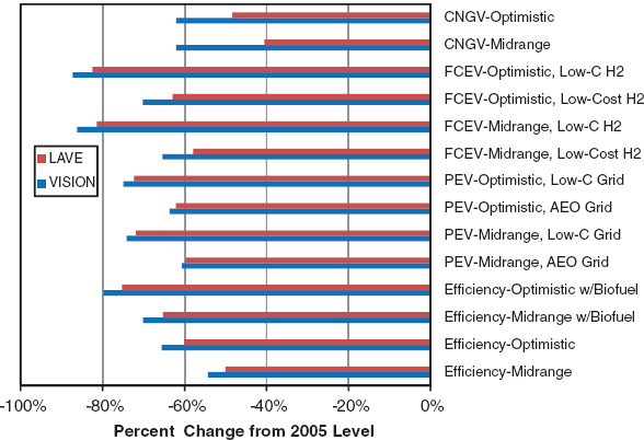
FIGURE 5.12 Comparison of LAVE-Trans and VISION model-estimated GHG reductions in 2050 given matching deployment.
tee elected to adopt the highest estimates of the Interagency Working Group on the Social Cost of Carbon (2010), and for petroleum reduction the committee derived its own estimates based on research by Leiby (2008) and others (see Box 5.5). These assumed values are shown in Figure 5.14.
Policies consistent with a strong commitment to reduce oil use and GHG emissions are included in all the policy cases. Specifically, a steady tightening of CAFE/GHG emissions standards combined with associated policies is assumed to ensure that they are met and enforced, which would yield efficiency improvements of both the midrange and optimistic vehicle technology scenarios, as explained in Chapter 2. Because the fuel economy and emissions standards will almost certainly be a binding constraint on manufacturers’ technology and design decisions, they will induce manufacturers to price the different drive train technologies so as to reflect their contributions to meeting the standards. This is represented by an approximately revenue-neutral feebate system that precisely reflects the social value of reductions in petroleum use and GHG emissions (see Boxes 5.3, 5.4, and 5.5 on feebates and the values of GHG and oil reduction).
Policies such as the RFS2, Low Carbon Fuels standards, or equivalent will be needed to bring drop-in biofuels to market, and additional policies will be required to ensure that electricity or hydrogen is produced via methods with
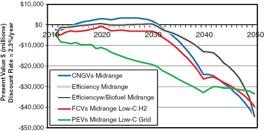
FIGURE 5.13 Annual subsidies to alternative fuels vehicles required to match five VISION cases. Negative values represent a net cost. The two efficiency curves are overlapping but not identical because the vehicle costs are the same and fuel costs nearly the same.
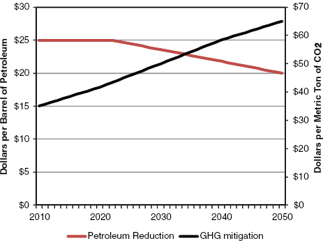
FIGURE 5.14 Assumed social values of reductions in GHG emissions and petroleum usage (in 2009$).
reduced greenhouse gas impacts, as explained in Chapter 3. These policies are implicit in all model runs except the BAU and Reference Cases. Their costs are reflected in the prices of the fuels for those cases assuming fuels produced with reduced GHG impacts (e.g., “+ Low-C Grid”). In addition, the very large improvements in energy efficiency included in all the policy runs will severely reduce Highway Trust Fund revenues unless measures are taken to prevent it. All policy cases assume that motor fuel taxes will be replaced by a user fee on energy (IHUF), indexed to the average energy efficiency of all vehicles on the road (see Chapter 6 for details).
Two additional fiscal policies were considered. A tax can be levied on fuels reflecting the social costs of their carbon emissions and petroleum content. When this tax is used, the feebates reflecting the social value of carbon emissions reductions are reduced. Since the vehicle choice model includes the first 3 years of fuel costs, the fuel taxes paid in those years will be taken into account by consumers in their vehicle purchase decisions. Thus, the feebate rates are adjusted to include only the social values of reductions in carbon emissions and oil use in the remaining years of the vehicle’s life. The impact of the fuel tax is therefore on vehicle use rather than vehicle choice. The remaining fiscal policy is an additional feebate system that compensates for consumers’ undervaluing of future fuel savings. This feebate reflects the discounted present value of fuel costs (excluding the social-cost fuel tax) from years 4 to 15, discounted to present value at 7 percent per year.10
5.4.2.1 Transition Policies
A transition to an alternative vehicle and fuel combination such as fuel cells and hydrogen or plug-in electric vehicles may be necessary to meet the reduction goals. This section focuses on such a transition away from the incumbent petroleum-based, ICEV-fuel system. As seen in the VISION results and again below, it may also be possible that the goals can be met without a transition to hydrogen- or electricity-powered vehicles. A shift away from petroleum fuel toward drop-in biofuels, combined with much more efficient ICEV and HEV engines, also offers an opportunity for significant greenhouse gas and petroleum reductions by 2050, although the 2030 petroleum reduction target remains difficult to achieve in all cases. With the data and model available, the committee is not able to fully explore the transition to large-scale low-carbon biofuels production here but does examine this case with the available information below.
In the LAVE model, transition polices consist of subsidies to vehicles and fuel infrastructure. These could be either direct government subsidies or subsidies induced by governmental regulations, such as California’s ZEV standards. The function of these subsidies is to allow alternative technologies to break through the market barriers that “lock-in” the incumbent petroleum-ICEV vehicle-fuel system. The transition policies used in the policy cases have been constructed by following these rules:
- Annual sales in the first 3 to 5 years of a transition should number in the thousands to tens of thousands of units.
- The increase in sales in any year should not be more than 6 percent of total light-duty vehicle sales.
_______________________
10OMB Circular No. A-94 recommends a discount rate for private return on capital of 7 percent (OMB, 2012).
- The growth of sales should avoid abrupt increases or decreases.
- Subsidies should be phased out as sales approach the level the market will support without subsidies.
In reality, a transition policy would need to be more comprehensive. Transition policies could potentially offer a greater variety of incentives, such as access to high occupancy vehicle lanes, free parking in congested areas, and so on. In the LAVE model the vehicle and fuel subsidies are intended to measure the cost of inducing transitions rather than to describe the specific polices by which they should be accomplished.
5.4.2.2 Transition Costs and Benefits
The costs and benefits of each of the policy cases presented below are measured relative to a Base Case that includes identical assumptions about technological progress and all other factors but does not include new policies to induce a transition to alternative vehicles or fuels or both. This was done to better measure the incremental costs and benefits of accomplishing transitions to alternative vehicles and fuels, as distinguished from the obvious benefits of having better technology. In general, this means that if the midrange technology assumptions are used in a transition case, the transition case will be compared to a Base Case that also uses the midrange technology assumptions. If a transition case uses optimistic assumptions for some technologies and midrange assumptions for others, its Base Case will make identical assumptions about technological progress. The transition cases differ from their respective Base Case only in terms of the transition policies. Except for the BAU and Reference Cases, all Base Cases assume that fuel economy and emissions standards are continuously tightened through 2050.
Costs and benefits are measured11 as changes from the respective Base Case in the following five quantities:
- Costs of subsidies,
- Additional fuel costs or savings,
- Changes in consumers’ surplus,
- The social value of GHG reductions, and
- The social value of reduced oil use.
- Subsidy costs include the implicit or explicit vehicle subsidies due to the higher costs of more efficient vehicles with lower greenhouse gas emissions, and they include the cost of subsidized infrastructure for public recharging of plug-in electric vehicles or refueling hydrogen or CNG vehicles.
- Additional fuel costs or savings. Since consumers are assumed to consider only the first 3 years of fuel savings in making their vehicles choices, it is necessary to account for the additional costs or savings over the remainder of each vehicle’s lifetime. Additional fuel costs or savings are private costs or benefits that accrue to the vehicle user that (by assumption) are not capitalized by the vehicle purchaser at the time of purchase.
- Consumers’ surplus is an economic concept that measures consumers’ welfare in dollars. Two changes in consumers’ surplus are measured: (1) satisfaction with vehicle purchases and (2) satisfaction with fuel purchases. The LAVE model includes a widely used method of modeling consumer choice that recognizes that not all consumers have the same tastes or preferences. Some may prefer the attributes of electric drive while others prefer internal combustion engines. If electric-drive vehicles become available at competitive prices as a result of successful transition policies, the satisfaction of those with a preference for electric drive will increase. Those who prefer ICEVs will still have that option and so will be no better or worse off than before the plug-in vehicles became available. Consumers’ surplus measures that increased value in dollars. Vehicle subsidies increase consumers’ surplus but by less than the gross amount of the subsidies. This results in a net economic cost, at least in the early years of a transition. Taxing the energy consumers must purchase to operate their vehicles creates a loss of consumers’ surplus, in addition to a transfer of wealth from consumers to the taxing entity. The surplus loss over and above what is counted in the vehicle purchase decision is also measured when changes in tax policies are considered.
- The social value of reducing greenhouse gas emissions and oil use. These values are measured by multiplying the changes in estimated annual quantities times the social cost of emissions per unit assumed by the committee consistent with the goals of the study (see Boxes 5.4 and 5.5). Hydrogen and fuel cell vehicles will also have zero tailpipe emissions of other pollutants, and may have lower full fuel cycle emissions, as well. The committee has not attempted to estimate those potential benefits, and they are not included in the cost and benefit estimates.
The net present value (NPV) of a policy case is the sum of all costs and benefits from 2010 to 2050, plus the fuel, GHG, and petroleum costs and benefits of vehicles sold through 2050 that will still be in use beyond that date. From an economic perspective, an optimal policy strategy would be one that maximized NPV. NPV depends strongly on the discount rate assumed, and there may be widely differing opinions about the appropriate discount rate. A 2.3 percent rate for
_______________________
11All costs and benefits are measured in constant dollars, discounted to present value using an annual discount rate of 2.3 percent.
all years is used, which is consistent with the most recent guidance of the U.S. government (OMB, 2012); however, the appropriate discount rate is yet another source of uncertainty.
Sections 5.4.3 to 5.4.9 present results from transition policy cases and compare them to their respective Base Cases. In general, all cases (except BAU and Reference) assume fuel economy/emissions standards to 2050. All cases (except BAU and Reference) include feebates and the IHUF. All transition cases assume vehicle subsidies or mandates and infrastructure subsidies or mandates. A few of the cases add special policies as noted in the text.
Rather than enabling us to reach definitive conclusions, the committee’s modeling suggests the extent of technological progress and the kinds and stringency of policy measures that are likely to be needed to bring about transitions. It provides useful insights about the interactions between policy, the market, and technological changes. It also provides a general indication of the costs and benefits of achieving the GHG and petroleum reduction goals conditional on the many assumptions that must be made. Uncertainty will be an inherent property of the process of energy transition: uncertainty about technological change, uncertainty about the market’s response to technologies and policies, and uncertainty about the future state of the world. The extent of uncertainty about both future technologies and the market’s response to them is illustrated by means of sensitivity analysis in Sections 5.6 and 5.7 below.
5.4.3 Energy Efficiency Improvement and Advanced Biofuels
The cases described in this section explore what may be possible given the midrange and optimistic technology projections, continued tightening of fuel economy and emissions standards, and large-scale production of thermo-chemically produced “drop-in” biofuels. These cases maintain the ICEVs with improved technology but involve a transition to large scale production and use of cellulosic biofuels. A final case also includes adoption of all the pricing policies described above. All cases include the IHUF, which increases from $0.42/gge in 2010 to $1.27/gge in 2050, and feebates that reflect the assumed societal willingness to pay for reductions in GHG emissions and oil use.
The technological progress enabling increased energy efficiency described in Chapter 2 (Table 2.11) will be devoted to improving vehicle fuel economy only if strong policies, such as increasingly stringent fuel economy and emissions standards, are put in place beyond 2025. The approximately revenue-neutral feebates, which are phased over 5 years beginning in 2017, amount to a tax of $60 per ICEV in 2021, with rebates of $770 per HEV, $1,650 per PHEV, $2,900 for each BEV, and $2,575 per FCEV. The feebates change over time as energy efficiencies, fuel properties, and the social willingness to pay for GHG and oil use reductions change. Assuming such standards are implemented, the midrange estimates of efficiency improvements and their costs result in estimated reductions in GHG emissions of 29 percent by 2030 and 52 percent by 2050 (Figure 5.15). For the same dates, petroleum consumption is estimated to be reduced by 33 and 64 percent, respectively. The reductions are due in part to the continued reduction in rates of fuel consumption for both ICEVs and HEVs (Figure 5.16) and by a steady shift from ICEVs to HEVs and BEVs (Figure 5.17).
If technology progresses as envisioned in the midrange scenario, the economic benefits of the efficiency improvements versus the Business as Usual case could be very large.
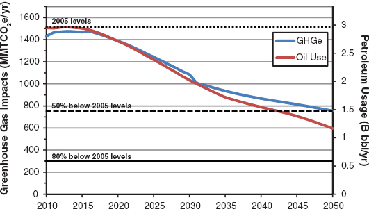
FIGURE 5.15 Changes in petroleum use and greenhouse gas (GHG) emissions for the Efficiency case with midrange technology estimates as compared to 2005 levels.
The key components of economic costs and benefits are shown in Figure 5.18 as annual costs, discounted to present value at the rate of 2.3 percent per year. The sum of the individual components grows to an estimated $130 billion per year by 2050. The largest component is “uncounted fuel savings,” the future fuel savings not considered by consumers at the time of purchasing a new car but realized later over the life of the vehicle. Consumers’ surplus, their net satisfaction with their vehicle purchases, decreases slightly after 2030 due to the increased cost of ICEVs over time. The net present social value of the transition to much higher efficiency vehicles is estimated to be on the order of $3.5 trillion.
Increasing the quantity of thermochemically produced, drop-in biofuels from 13.5 billion gge to 19.2 billion gge in 2030 increases the estimated reduction in petroleum use from 33 to 37 percent in that year. The 2030 reduction in GHG emissions is 32 percent versus 28 percent. In 2050, when the biofuels industry has expanded to produce 45 billion gge, the estimated impact is much greater: petroleum use is down 86 percent (compared with 64 percent) and GHG emissions are 66 percent lower than in 2005 (compared with 52 percent without advanced biofuels) (Figure 5.19).
If carbon emissions from the production of 20 percent of thermochemical biofuels were captured and stored, an estimated 78 percent reduction in GHG emissions versus
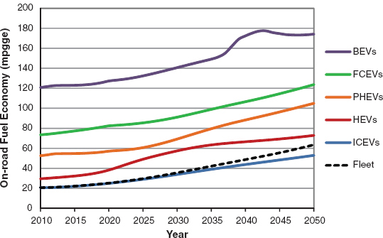
FIGURE 5.16 Average fuel economy of on-road vehicles for the Efficiency case with midrange technology estimates. The upturn in battery electric vehicle (BEV) fuel economy after 2040 reflects the rapidly increasing share of new BEVs on the road (and thus a larger fraction of the BEV fleet is the newest, most efficient BEVs). The downturn that follows is representative of an increasing number of battery electric trucks in the fleet.
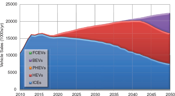
FIGURE 5.17 Vehicles sales by vehicle technology for the Efficiency case with midrange technology estimates.
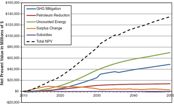
FIGURE 5.18 Estimated costs and benefits for the Efficiency case with midrange technology estimates.
2005 could be achieved by 2050. Given the uncertainty in the analysis, the 2050 goals would then be met for all practical purposes. The 2030 goal of a 50 percent reduction in petroleum use is still missed because of the low initial ramp-up in production, however; the estimated reduction is 37 percent. The cost of 20 percent CO2 removal for biofuels blended into gasoline adds about $0.20 per gallon to the average price of gasoline in 2050. If CCS is applied to all biofuels, then the net GHG emissions from the LDV fleet could be slightly negative.
5.4.4 Emphasis on Pricing Policies
A great deal can be accomplished by means of policies that change the prices of fuels and vehicles and harness market forces to reduce GHG emissions. This scenario, like the others based on the midrange technology scenario, assumes that fuel economy standards are inducing manufacturers to produce increasingly efficient vehicles. However, it also introduces stronger feebates and adds to the cost of fuels the social willingness to pay for GHG and oil reduction. The additional feebate system capitalizes in vehicles’ prices the uncounted energy savings due to consumers’ assumed under-
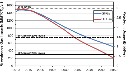
FIGURE 5.19 Changes in petroleum use and greenhouse gas (GHG) emissions for the Efficiency + Biofuels case as compared to 2005 levels.
valuing of future fuel savings.12 Production of electricity and hydrogen via processes with low-GHG impacts is assumed, but not intensive use of drop-in biofuels.
The fully taxed price of gasoline increases from $2.70 per gallon in 2010 to $4.90 per gallon in 2020 and $5.50 per gallon in 2030. Gasoline prices continue to increase, reaching $6.60 per gallon in 2050, as a result of $2.70 per gallon in combined taxes. The price of electricity in 2050 is roughly equal to that of gasoline on an energy basis, but BEVs are more than three times more energy efficient than comparable ICEVs in 2050. Feebates also strongly encourage purchases of BEVs. The rebate for a BEV in 2020 is almost $14,000, while ICEVs are taxed at $300 each. The difference decreases as vehicles and fuels improve so that by 2050, BEVs receive a $1,300 per vehicle rebate, whereas ICEVs are taxed at $2,500 per vehicle (the incidence also shifts to approximate revenue neutrality).
The result is a massive shift to battery electric and hybrid electric vehicles. By 2050, an estimated 59 percent of new-vehicle sales are BEVs and 33 percent are HEVs. In 2050 almost 40 percent of the vehicles on the road are BEVs. In the absence of policies to put a hydrogen refueling infrastructure in place, fuel cell vehicles never achieve any significant share of the market. Battery electric vehicles are far less dependent on early infrastructure development, which gives them a decisive advantage over FCEVs in this scenario.
Light-duty vehicle petroleum use is estimated to be 38 percent lower than the 2005 level by 2030, and 87 percent below 2005 in 2050. Greenhouse gas emissions are reduced 74 percent by 2050. Vehicle miles of travel in 2050 are also more than 15 percent lower than in the Efficiency Case (identical assumptions but without the additional pricing policies). In part this is due to the higher energy prices, but it is also due to 7 percent fewer vehicles on the road and lower annual miles for the 39 percent of vehicles that are BEVs.
5.4.5 Plug-in Electric Vehicles
Plug-in electric vehicles (PEVs) possess some attributes that are substantially different from those of the other vehicle types. Battery electric vehicles (BEVs) not only have limited range but also have long recharging times. The combination of these two attributes limits the ability of BEVs to satisfy all the daily travel demands of most drivers. This reduces the total annual mileage of BEVs to two thirds of that of an ICEV, HEV, CNGV, or FCEV and detracts from their utility to most households. In the LAVE-Trans model, most but not all of the vehicle travel demand that cannot be satisfied by BEVs is shifted to other vehicles in the vehicle stock. To some degree the BEV’s travel range limitations will be offset by its lower energy costs. In the midrange technology scenario, the long-run, fully learned cost of BEVs is $20,000 more than that of ICEVs in 2010, although BEVs eventually become $600 less expensive by 2050 (see Figure 5.8). PHEVs, on the other hand, suffer no such limitations on use and can take energy from the grid or from the gas pump. However, their initial cost is higher and remains higher through 2050 in the midrange scenario. PHEVs start out with a high-volume, learned cost that is $10,000 more than that of an ICEV and remains at least $2,000 more expensive through 2050. The PHEV’s higher price will be partly offset by lower energy costs, yet its price remains a significant barrier to full market success.
Two PEV transition policy scenarios are reported below. Both include feebates reflecting social willingness to pay for GHG and petroleum reduction plus the IHUF. In the first, PHEVs achieve a modest market share of 5 percent whereas BEVs account for 35 percent of new-car sales by 2050. The scenario continues the current levels of PHEV and BEV sales, which requires substantial, sustained subsidies: total subsidies per BEV decrease from $25,000 per vehicle in 2012 to just over $10,000 per vehicle in 2020.13 When long-run PEV costs approach the prices of other technologies the transitional subsidies are removed (2028 for BEVs and 2033 for PHEVs) but the feebates and IHUF continue. By 2050, PEVs constitute 40 percent of the market, HEVs 34 percent, and advanced ICEVs 26 percent (Figure 5.20). In this case, petroleum use is 35 percent lower than the 2005 level in 2030 and 73 percent lower in 2050. GHG emissions are 31 and 63 percent below the 2005 level in 2030 and 2050, respectively. If the AEO 2011 reference grid assumptions are used, the GHG reductions are 31 percent in 2030 and 56 percent in 2050.
Despite the cost of vehicle subsidies (over $50 billion present value) this scenario still has a substantial positive net present value of over $500 billion. Most of the benefits (about 50 percent) are due to uncounted energy savings from PEVs, which have substantially lower energy costs than ICEVs or HEVs (Figure 5.21).
Adding greater volumes of advanced biofuels (45 billion gge in 2050) to the PEV Transition Policy case reduces petroleum use relative to 2005 by 40 percent in 2030 and 94 percent in 2050. The GHG reductions in those years are estimated to be 34 and 75 percent assuming electricity generated by a low-carbon grid.
As described above, the initial costs for PEVs are substantially higher than for other technologies, primarily due to battery costs. If subsidies are not applied until battery costs have come down significantly, there is still opportunity for significant benefits. If the current advanced vehicle tax credits are allowed to expire in 2020, it is possible to induce a transition
_______________________
12It is likely that the feebates alone would induce manufacturers to realize fuel economy and emissions improvements similar to those assumed to result from standards, but that possibility has not been tested here (Greene et al., 2005).
13These estimated total subsidies may appear too high given a federal tax credit of only $7,500 for BEVs and $5,000 for PHEV-30s. However, states also offer incentives of up to $7,500, and manufacturers are very likely also subsidizing initial sales, partly to induce market success and partly to gain credits under the CAFE regulations and ZEV mandates.
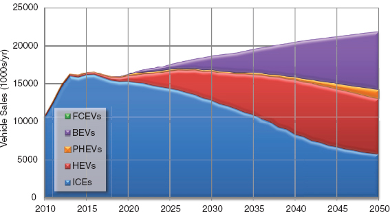
FIGURE 5.20 Vehicle sales by vehicle technology assuming midrange technologies and plug-in electric vehicle subsidies and additional incentives.
to PEVs by 2050 while waiting to apply technology-specific subsidies to PEVs until 2023. These subsidies are complemented by the usual IHUF and feebates. In this case, the total subsidy to BEVs is $13,000 per passenger car in 2023. However, it is reduced to $6,000 per vehicle by 2028, and by 2034 only the feebate remains. A similar subsidy trajectory is followed for PHEVs but is delayed by 6 years, beginning instead in 2029 after vehicle costs have been further reduced. By 2050, BEVs make up 35 percent of new-vehicle sales, while PHEVs are 6 percent, both shares similar to the cases by Vehicle Technology above. Likewise, petroleum usage in 2030 is reduced by 34 percent, and petroleum usage and GHG emissions in 2050 are reduced by 73 and 63 percent, respectively, compared to 2005 levels; these are almost identical to the PEV transition case without biofuels but with the low-carbon grid, discussed above. The net present value is nearly identical ($520 billion compared to $540 billion), and the total cost of the subsidies necessary to produce the transition are essentially the same, as well, $50 billion.
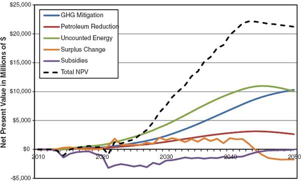
FIGURE 5.21 Estimated costs and benefits of the transition to 25 percent plug-in electric vehicles (PEVs) assuming midrange technologies and PEV subsidies and additional incentives.
5.4.6 Hydrogen Fuel Cell Electric Vehicle Cases
Given the midrange technology assumptions, if no early hydrogen infrastructure is provided and the existing tax credits are allowed to expire in 2020, a transition to FCEVs does not occur. An early transition to hydrogen fuel cell vehicles can be induced by ensuring that an adequate amount of hydrogen refueling infrastructure to support early vehicle sales is in place at least in some regions ahead of vehicle sales and that vehicle subsidies or mandates support early sales. All the FCEV transition cases include feebates reflecting social willingness to pay for GHG and oil reduction and the IHUF. The three carbon-intensity cases described in Chapter 3 were tested, beginning with low-cost hydrogen produced mainly by steam methane reforming without carbon capture and storage.
The first FCEV transition case assumes that 200 subsidized or mandated hydrogen refueling stations are put in place in 2014, 200 in 2015, and 100 more in 2016. These stations are likely to be geographically clustered, for example, in California and other states where ZEV requirements and other supporting policies are in place. Increased hydrogen vehicle subsidies (or mandates inducing implicit subsidies) begin in 2015 at $17,500 per vehicle (including the existing tax credit). The initial, high subsidies decline gradually to $16,000 per vehicle in 2020 and $6,000 by 2025. This induces modest levels of FCEV sales: 9,000 in 2015, followed by annual sales of 16,000, 21,000, and 26,000 in 2016-2018 (Figure 5.22). The transitional vehicle subsidy is ended in 2027, but the feebate system that in 2027 provides a $1,400 rebate for FCEVs and imposes a $500 tax on ICEVs remains in effect. By 2050, almost half of the vehicles on the road are FCEVs or HEVs.
In the low-cost hydrogen case, petroleum consumption is estimated to be 41 percent below the 2005 level in 2030. In 2050 petroleum consumption is down an estimated 90 percent relative to 2005 and GHG emissions are 59 percent lower. Assuming CCS is used in the production of hydrogen, greenhouse gas emissions are estimated to be 74 percent lower in 2050 and petroleum use is 95 percent below the 2005 level (Figure 5.23). Using assumptions to produce hydrogen with the lowest GHG impacts, 2050 GHG emissions are estimated to be 80 percent lower than in 2005, and petroleum use 96 percent below the 2005 level. Petroleum use in 2030 is estimated to be 42 percent below 2005 in this case. With the feebates in place, the higher-cost but lower-GHG-impact hydrogen increases FCEV sales: in the low-carbon production case FCEVs take an estimated 57 percent of the market in 2050, and in the low-cost production hydrogen case they capture 48 percent.
Despite the initial cost of subsidies that reach $6 billion per year in the mid-2020s, the estimated net present value of the policy-induced transition to hydrogen FCEVs is on the order of $1 trillion (Figure 5.24). The benefits are roughly equally composed of social benefits (GHG and petroleum reduction) and private benefits (fuel savings and consumers’ surplus gains).
Adding advanced biofuels to the FCEV policy case reduces the 2050 market share of FCEVs from 57 to 46 percent. Low-GHG gasoline reduces the cost penalty that feebates levy on ICEVs; vehicles consuming drop-in biofuel instead of petroleum gasoline become more cost-competitive with FCEVs and gain market share. This is an illustration of how policies may interact in ways that make the combined impact smaller than the sum of the individual effects. Still, total petroleum use and GHG emissions are lower. In 2030, petroleum use is estimated to be 46 percent below the 2005 level and GHG emissions are 37 percent below (versus 42 and 35 percent, respectively, without advanced biofuels). In 2050, adding advanced biofuels reduces GHG emissions to 86 percent below the 2005 level and petroleum use to 100 percent below.
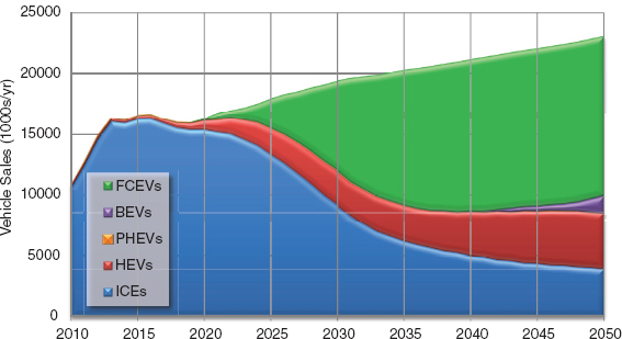
FIGURE 5.22 Vehicle sales by vehicle technology with midrange technology assumptions and low-carbon production of hydrogen, fuel cell vehicle subsidies, and additional incentives.
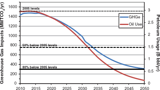
FIGURE 5.23 Changes in petroleum use and greenhouse and (GHG) emissions with midrange technology assumptions, fuel cell vehicle subsidies and additional incentives, and a low-GHG infrastructure for the production of hydrogen.
5.4.7 Compressed Natural Gas Vehicles
Due to limitations of the LAVE model, CNGVs take the place of FCEVs; FCEVs are excluded from analyses in which CNGVs are included. Like FCEVs, only one type of CNGV is considered, CNG non-hybrid ICEVs. CNGVs have some advantages relative to other advanced technologies. Natural gas prices are lower than petroleum, biofuel, or hydrogen prices, and the infrastructure for natural gas production and distribution is nearly ubiquitous. This means that, unlike hydrogen, there is no initial phase of high prices at low volumes. Natural gas refueling stations are still required, however, and natural gas vehicles have lower range than gasoline vehicles due to the lower energy density of CNG. The CNG policy case includes feebates and the IHUF, both commencing in 2015. Also in that year there is a transitional subsidy/mandate of $10,000 per CNGV. Like the vehicle subsidies in other cases, this could be borne by the manufacturer or government or shared between the two. The transitional subsidy is reduced each year and ended by 2025. In addition, 100 subsidized refueling stations are opened in 2014, 200 in 2015, and 100 more in 2016. CNGV sales peak at 49 percent from 2031-2034, then decline to 33 percent in
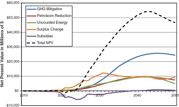
FIGURE 5.24 Present value cost and benefits of a transition to hydrogen fuel cell vehicles using midrange technology assumptions, fuel cell vehicle subsidies and additional incentives, and a low-GHG infrastructure for the production of hydrogen.
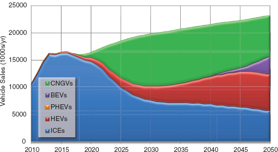
FIGURE 5.25 Vehicle sales by vehicle technology for midrange technology estimate and policies promoting compressed natural gas vehicles.
2050 (Figure 5.25), chiefly due to the feebates which favor BEVs and even HEVs and ICEVs over CNGVs.
In the CNG transition policy case, petroleum consumption is estimated to be 52 percent below the 2005 level in 2030. GHG emissions are 28 percent lower. In 2050, estimated petroleum use and GHG emissions are, respectively, 86 and 47 percent lower than 2005 levels (Figure 5.26). Adding advanced biofuels to the CNG transition case eliminates petroleum use in 2050 and reduces GHG emissions to an estimated 62 percent below the 2005 level. If it is assumed that some CNGVs will be hybrid vehicles, the model would suggest no more than a few additional percent reductions in GHG emissions because these CNG HEVs would not be further displacing gasoline-powered vehicles but rather less efficient CNG ICEVs. All greenhouse gas emissions for natural gas vehicles are strongly predicated on the methane leakage rates outlined in Chapter 3 due to methane’s large global warming potential.
5.4.8 Plug-in Electric Vehicles and Hydrogen Fuel Cell Electric Vehicles
Combining subsidies to PEVs and FCEVs with advanced biofuels and also including the usual feebates and IHUF on energy eliminates petroleum use in 2050 and reduces GHG emissions by 88 percent versus 2005 levels. In 2030, a 56 percent reduction in petroleum use is achieved. The implied subsidies required to achieve this result are substantial. In 2015, a BEV gets a total subsidy of $20,500; a FCEV, $27,500; and a PHEV, $13,000. The implied subsidies decrease to about $3,000 per BEV and FCEV and half of that for PHEVs in 2025, including feebates. After
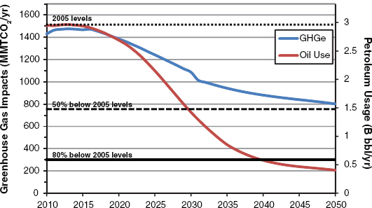
FIGURE 5.26 Changes in petroleum use and greenhouse gas emissions for midrange technology estimates with policies promoting compressed natural gas vehicles.
2030 the transitional subsidies are ended but the feebates remain. The total NPV of subsidies is approximately $140 billion. Although both technologies attain sustainable market shares, they compete with one another as well as with ICEVs and HEVs, which reduces their combined impact (Figure 5.27). The presence of several competing technologies in the marketplace tends to limit diversity of choice (fewer makes and models for any given technology) and to a lesser extent reduces fuel availability (due to fewer vehicles of any one type on the road), in comparison to a case dominated by one or two technologies. Nonetheless, this case achieves a NPV gain of $1.7 trillion versus the same technology assumptions without policy interventions to induce transitions. In this case, all of the liquid fuel used by vehicles with internal combustion engines is biofuel. In addition, the grid is low-carbon, as is hydrogen production. As a result, by 2050, there is almost no difference in the social costs (GHGs and petroleum use) of the different powertrain technologies. No vehicle receives a fee or a rebate that exceeds $50.
5.4.9 Optimistic Technology Scenarios
Optimistic technology scenarios imply breakthrough advancement of a given technology. These are taken to represent roughly a 20 percent likelihood occurrence in technological development for the respective technology. Such advancement is less likely than the midrange assumptions, although if it occurs, it changes the landscape for adoption of a technology, both in its costs and its benefits. In brief, the optimistic technology cases show that better-than-anticipated progress for plug-in vehicle technology combined with a decarbonized grid and assuming the same policies spelled out for the midrange cases above could come close to achieving the GHG and petroleum reduction goals by 2050 but fall short of the 2030 petroleum use goal. A parallel case for fuel cell vehicles could achieve or exceed all of the goals. A full explanation of the optimistic cases is contained in Section H.4 in Appendix H.
5.4.10 Summary of Policy Modeling Results
The results of all the cases are summarized and compared in Tables 5.3 and 5.4 and in Figures 5.28 and 5.29. The fuel infrastructure investment costs modeled to achieve each scenario can be found in Section H.3 in Appendix H. The cases in Tables 5.3 and 5.4 are grouped in the same order as the case descriptions above. Abbreviations used in the table are explained in Table 5.5. For each group, there is a Base Case using the identical vehicle technology assumptions but without energy transition policies. All cases, including the Base Cases, assume policies requiring continued improvements in vehicle energy efficiencies and, therefore, all cases also include feebates consistent with the fuel economy and emissions standards. The inherent uncertainties in the model estimates should be kept in mind.
Only three cases are estimated to meet or exceed the 50 percent petroleum reduction goal in 2030 and the 80 percent petroleum and GHG reduction goals in 2050. One is based on optimistic assumptions for FCEV technology; the other two require both plug-in and hydrogen fuel cell market success, plus the low-carbon production of electricity and hydrogen, and the supporting policies of fuel economy/emissions standards and the IHUF on energy.
Two additional cases meet the 2030 petroleum goal but miss the 2050 GHG goal by wide margins. Both cases are based on a substantial transition to CNGVs, and such a transition may result in even more greenhouse gas emissions than modeled due to uncertainty in methane leakage rate and methane’s substantial greenhouse warming potential. Eight cases are in the range of 40 to 50 percent petroleum reduction in 2030. Given the uncertainty inherent in the
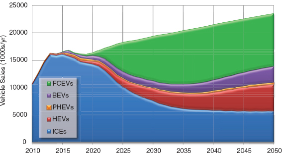
FIGURE 5.27 Vehicle sales by vehicle technology for midrange technologies and policies promoting the adoption and use of plug-in electric vehicles, hydrogen fuel cell electric vehicles, and biofuels.
TABLE 5.3 Summary of Estimated Petroleum and GHG Reductions in the Policy Cases
| Oil Reduction (% reduction below 2005 level) | GHG Reduction (% reduction below 2005 level) | Oil Consumption (billion bbl/yr) 2005 = 2.96 | GHG Emissions (MMTCO2e/yr) 2005 = 1514 | ||||||
| Scenarioa | 2030 | 2050 | 2030 | 2050 | 2030 | 2050 | 2030 | 2050 | |
| BAU | −5% | 4% | −3% | 9% | 2.8 | 3.1 | 1,467 | 1,645 | |
| Reference | −29% | −27% | −26% | −22% | 2.1 | 2.2 | 1,118 | 1,184 | |
| Eff+FBSC | −32% | −61% | −29% | −50% | 2.0 | 1.2 | 1,082 | 755 | |
| Eff+FBSC+IHUF | −33% | −64% | −29% | −52% | 2.0 | 1.1 | 1,071 | 721 | |
| Eff+Bio+FBSC+IHUF | −37% | −86% | −32% | −66% | 1.9 | 0.4 | 1,030 | 508 | |
| Eff+Bio w/CCS+FBSC+IHUF | −37% | −86% | −35% | −78% | 1.9 | 0.4 | 979 | 335 | |
| Eff+Intensive Pricing+LCe | −38% | −87% | −35% | −74% | 1.8 | 0.4 | 990 | 389 | |
| PEV+ FBSC+IHUF+Trans+AEOe | −35% | −71% | −31% | −56% | 1.9 | 0.9 | 1,049 | 662 | |
| PEV+ FBSC+IHUF+Trans+LCe | −35% | −73% | −31% | −63% | 1.9 | 0.8 | 1,046 | 567 | |
| PEV(later)+FBSC+IHUF+Trans+LCe | −34% | −73% | −30% | −63% | 2.0 | 0.8 | 1,055 | 563 | |
| PEV+Bio+FBSC+IHUF+Trans+LCe | −40% | −94% | −34% | −75% | 1.8 | 0.2 | 1,005 | 381 | |
| FCEV+FBSC+IHUF+Trans+L$H2 | −41% | −91% | −32% | −59% | 1.7 | 0.3 | 1,025 | 621 | |
| FCEV+FBSC+IHUF+Trans+H2CCS | −42% | −95% | −34% | −74% | 1.7 | 0.1 | 993 | 391 | |
| FCEV+FBSC+IHUF+Trans+LCH2 | −42% | −96% | −35% | −80% | 1.7 | 0.1 | 982 | 310 | |
| FCEV+Bio+FBSC+IHUF+Trans+LCH2 | −46% | −100% | −37% | −86% | 1.6 | 0.0 | 949 | 209 | |
| CNGV+FBSC | −32% | −61% | −29% | −50% | 2.0 | 1.2 | 1,082 | 755 | |
| CNGV+FBSC+IHUF+Trans | −52% | −86% | −28% | −47% | 1.4 | 0.4 | 1,086 | 801 | |
| CNGV+Bio+FBSC+IHUF+Trans | −56% | −100% | −31% | −62% | 1.3 | 0.0 | 1,045 | 568 | |
| Eff (Opt)+FBSC | −38% | −68% | −34% | −59% | 1.8 | 0.9 | 1,000 | 620 | |
| Eff (Opt)+Bio+FBSC+IHUF | −43% | −95% | −37% | −76% | 1.7 | 0.2 | 947 | 367 | |
| PEV (Opt)+FBSC+AEOe | −32% | −78% | −29% | −60% | 2.0 | 0.7 | 1,082 | 607 | |
| PEV (Opt)+FBSC+IHUF+Trans+LCe | −35% | −89% | −31% | −76% | 1.9 | 0.3 | 1,048 | 368 | |
| FCEV (Opt)+FBSC+L$H2 | −32% | −61% | −29% | −50% | 2.0 | 1.2 | 1,082 | 755 | |
| FCEV (Opt)+FBSC+IHUF+Trans+LCH2 | −50% | −100% | −41% | −90% | 1.5 | 0.0 | 888 | 150 | |
| PEV+FCEV+FBSC+IHUF+Trans+LCe+LCH2 | −52% | −99% | −42% | −82% | 1.4 | 0.0 | 872 | 267 | |
| PEV+FCEV+Bio+FBSC+IHUF+Trans+LCe+LCH2 | −56% | −100% | −45% | −87% | 1.3 | 0.0 | 839 | 190 | |
aBase Cases are indicated in boldface. Eff+FBSC serves as a Base Case for the four groups below it: Eff, Intensive Pricing, PEV, and FCEV, as well as for the mixed cases in the final grouping including both PEVs and FCEVs. See Table 5.5 for explanation of scenario components.
modeling analysis, that may be close enough. All of these cases meet the 2050 petroleum reduction goal. Six of the eight cases achieving an estimated 40 percent or greater reduction in petroleum use by 2030 also achieve a 70 percent or greater reduction in GHG emissions by 2050. Three are based on hydrogen fuel cell market success; one combines plug-in vehicle market success with biofuels. One relies on efficiency plus greater use of pricing policies, but this also induces a massive shift to plug-in vehicles by 2050. The final case combines optimistic efficiency improvements with biofuels to achieve an estimated 76 percent reduction in GHG emissions in 2050.
All five cases that meet the 2050 GHG reduction goal also imply near elimination of petroleum use. This is likely to be more difficult than the modeling analysis makes it appear. Near elimination of U.S. petroleum use, if it is also accomplished by other petroleum using countries, would cause world petroleum prices to fall. Falling petroleum prices have not been included in the modeling analysis but would make it more difficult for alternative technologies to succeed. This effect could be countered by a policy setting a price floor on petroleum, as discussed in Chapter 6.
As uncertain as these estimates are, they provide several important insights. First, reaching the 2030 and 2050 goals will be difficult. It will require strong and sustained policies to continuously improve the energy efficiency of LDVs and to de-carbonize the systems supplying energy for the vehicles, and very likely it will also require strong policies to induce a transition to one or more of the advanced power-train technologies. Second, continued improvement in vehicle and fuel technologies is essential. Although the committee considers the technological progress assumed in the committee’s scenarios to be reasonably likely, it is not guaranteed. Given that several technological advances are necessary to come close to meeting the goals, research and development of all the technologies considered in this report is a high priority.
If the alternative technologies develop and are deployed according to the committee’s technological and market assumptions, the scenario modeling indicates that the additional costs of any transition may be much smaller
TABLE 5.4 Total Net Present Value in 2050 for Various Cases
| Scenarioa | Net Present Value (billions $) | ||||||||
| Surplus Change | Subsidies | GHG Mitigation | Petroleum Reduction | Uncounted Energy | Total NPV | ||||
| BAU | 0.0 | 0.0 | 0.0 | 0.0 | 0.0 | 0.0 | |||
| Reference | 0.0 | 0.0 | 0.0 | 0.0 | 0.0 | 0.0 | |||
| Eff+FBSC | 0.0 | 0.0 | 0.0 | 0.0 | 0.0 | 0.0 | |||
| Eff+FBSC+IHUF | −7.0 | −0.8 | 44.6 | 16.6 | 78.2 | 131.7 | |||
| Eff+Bio+FBSC+IHUF | −20.0 | 4.8 | 285.6 | 151.0 | 49.0 | 470.3 | |||
| Eff+Bio w/CCS+FBSC+IHUF | −40.7 | 6.5 | 507.8 | 150.5 | 48.0 | 672.2 | |||
| Eff+Intensive Pricing+LCe | −361.3 | −128.0 | 520.1 | 253.4 | 1103.4 | 1387.5 | |||
| PEV+ FBSC+IHUF+Trans+AEOe | 43.0 | −53.3 | 136.3 | 72.6 | 285.5 | 484.2 | |||
| PEV+ FBSC+IHUF+Trans+LCe | 23.8 | −52.3 | 218.9 | 76.6 | 273.8 | 540.7 | |||
| PEV(later)+FBSC+IHUF+Trans+LCe | 29.2 | −50.6 | 212.6 | 72.3 | 259.6 | 523.2 | |||
| PEV+Bio+FBSC+IHUF+Trans+LCe | 24.7 | −45.7 | 437.1 | 205.6 | 226.8 | 848.6 | |||
| FCEV+FBSC+IHUF+Trans+L$H2 | 307.0 | −38.6 | 210.3 | 200.4 | 287.0 | 965.9 | |||
| FCEV+FBSC+IHUF+Trans+H2CCS | 279.7 | −44.0 | 493.0 | 222.6 | 289.0 | 1240.3 | |||
| FCEV+FBSC+IHUF+Trans+LCH2 | 252.9 | −45.7 | 591.2 | 225.3 | 198.0 | 1221.7 | |||
| FCEV+Bio+FBSC+IHUF+Trans+LCH2 | 276.2 | −38.5 | 725.1 | 275.4 | 56.9 | 1295.1 | |||
| CNGV+FBSC | 0.0 | 0.0 | 0.0 | 0.0 | 0.0 | 0.0 | |||
| CNGV+FBSC+IHUF+Trans | 414.3 | −32.7 | −40.1 | 248.1 | 251.1 | 840.7 | |||
| CNGV+Bio+FBSC+IHUF+Trans | 396.0 | −31.1 | 222.4 | 346.9 | 210.6 | 1144.7 | |||
| Eff (Opt)+FBSC | 0.0 | 0.0 | 0.0 | 0.0 | 0.0 | 0.0 | |||
| Eff (Opt)+Bio+FBSC+IHUF | −20.1 | 2.5 | 291.7 | 153.5 | 60.2 | 487.8 | |||
| PEV (Opt)+FBSC+AEOe | 0.0 | 0.0 | 0.0 | 0.0 | 0.0 | 0.0 | |||
| PEV (Opt)+FBSC+IHUF+Trans+LCe | 18.0 | −54.1 | 280.7 | 79.2 | 299.6 | 623.4 | |||
| FCEV (Opt)+FBSC+L$H2 | 0.0 | 0.0 | 0.0 | 0.0 | 0.0 | 0.0 | |||
| FCEV (Opt)+FBSC+IHUF+Trans+LCH2 | 596.0 | −47.0 | 869.4 | 294.2 | 590.3 | 2302.9 | |||
| PEV+FCEV+FBSC+IHUF+Trans+LCe+LCH2 | 345.0 | −145.3 | 739.8 | 300.8 | 442.0 | 1682.3 | |||
| PEV+FCEV+Bio+FBSC+IHUF+Trans+LCe+LCH | 371.7 | −137.4 | 855.8 | 340.6 | 264.8 | 1695.5 | |||
aBase Cases are indicated in boldface. Eff+FBSC serves as a Base Case for the four groups below it: Eff, Intensive Pricing, PEV, and FCEV, as well as for the mixed cases in the final grouping including both PEVs and FCEVs. See Table 5.5 for explanation of scenario components.
than the sum of private and public benefits. The benefits considered in the model include both public and private benefits such as benefits to the owners of the vehicles (i.e., the uncounted energy savings), benefits to the owners of all vehicles (i.e., the increased consumer surplus), and benefits to society at large (the benefits of GHG emissions reduction and reduced petroleum use). Costs refer to the additional costs of the transition over and above what the market is willing to do voluntarily, as represented by the respective Base Case. These include any increases in vehicle or fuel costs not included in consumers’ surplus, net subsidies, and consumers’ surplus losses. If there were increases in GHG emissions or petroleum use, these would also be included in transition costs.
5.5 COMPARISON TO PREVIOUS WORK
The LAVE-Trans modeling represents a significant step toward more completely modeling scenarios by which the LDV fleet could be drastically changed. However, because of the uncertainties concerning the behavior of consumers and firms that underpins these modeling results as well as the uncertainty in projected costs and available technologies, it is important to consider these results in the context of the large body of literature on transitions to alternative vehicles and fuels. Here the focus is on some of the key findings and assumptions of the modeling compared to the available literature; a detailed summary of key reports on the matter is given in Appendix D.
A number of policy scenarios modeled above include the use of a large volume of biofuels (up to 45 billion gge/yr) in order to meet the goals for petroleum reduction and/or GHG emissions reductions from the LDV fleet. As is described in Chapter 3, the biomass required for such volumes of cellulosic drop-in fuel is plausible; many previous studies indicate a similar level of available biomass resource (UCD, 2011; NRC, 2008, 2009b; DOE, 2011; Greene and Plotkin, 2011; Pacala and Socolow, 2004). However, there is still uncertainty about the levels of production necessary to contribute significantly to the fueling of the LDV fleet due to the unknown future cost of fuels produced from biomass relative to gasoline produced from petroleum (DOE, 2011).
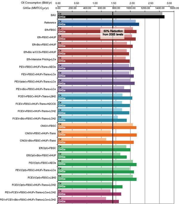
FIGURE 5.28 Estimated petroleum usage and greenhouse gas emissions in 2030, by policy scenario. Hydrogen fuel cell electric vehicle (FCEV) and plug-in electric vehicle (PEV) scenarios Utilize Low-Carbon production of alternative fuel unless otherwise specified. See Table 5.5 for explanation of scenario components.
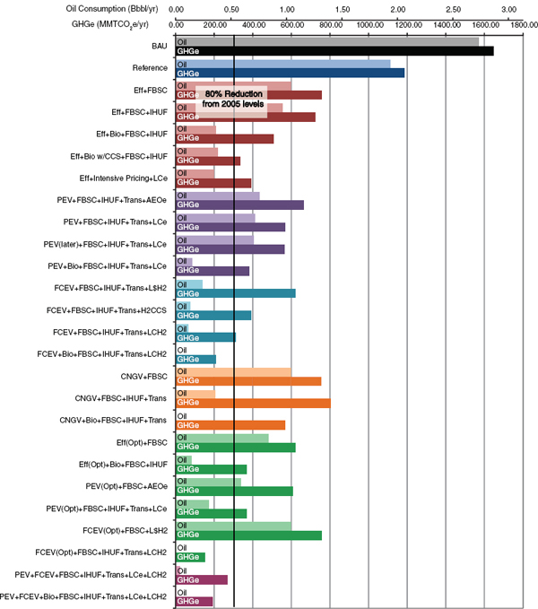
FIGURE 5.29 Estimated petroleum usage and greenhous gas emissions 2050, by policy scenario. Hydrogen fuel cell electric vehicle (FCEV) and plug-in electric vehicle (PEV) scenarios utilize Low-Carbon production of alternative fuel unless otherwise specified. See Table 5.5 for explanation of scenario components.
TABLE 5.5 Abbreviations for Policies Considered in the LAVE-Trans Model
| Eff | Improved vehicle efficiency—midrange technology assumptions |
| FBSC | Feebates based on societal willingness to pay for GHG and petroleum reduction |
| IHUF | User fee on energy indexed to the average energy efficiency of all on-road vehicles |
| Bio | Assumes increased use of thermochemical biofuels up to 45 billion gge in 2050 |
| CCS | Includes the use of carbon capture and storage |
| Intensive | Includes IHUF, FBSC, carbon/oil tax, and feebates based on |
| pricing | fuel savings (see Sections 5.4.2 and 5.4.4) |
| Trans | Transition policies consisting of vehicle and fuel infrastructure subsidies or mandates |
| AEOe | Reference Case electricity grid based on Annual Energy Outlook 2011 |
| LCe | Low-Carbon electricity grid |
| L$H2 | Low-Cost production of hydrogen |
| H2CCS | Production of hydrogen with Carbon Capture and Storage |
| LCH2 | Low-Carbon production of hydrogen |
| (Opt) | Optimistic technology assumptions for the indicated technology (see Section H.4 in Appendix H for details) |
NOTE: For more details on fuels production, see Table 5.1 and Chapter 3. Vehicle technology assumptions are described in Chapter 2. Policies are defined in Box 5.2.
A further limit on the availability of biofuels is likely to be competition from other uses, such as in aircraft or heavy-duty vehicles (UCD, 2011). Such limited availability would prevent achievement of an 80 percent reduction in GHG emissions without advanced progress in hydrogen fuel cell technology. A UC-Davis report noted that biofuels would play a pivotal role in any policy scenario designed to reduce GHG emissions from the transportation sector, particularly in the next two decades while deployment of advanced powertrain vehicles is still in its infancy (Yeh et al., 2008). The committee accepted as a premise in its modeling the achievement by 2030 of the production of volumes of biofuel specified in RFS2 and did not examine scenarios in which biofuel deployment did not achieve these levels.
As can be seen from the midrange cases in Figure 5.29, improvements in vehicle efficiency, particularly when combined with policies to drive consumers to purchase efficient vehicles, offer the possibility of large reductions in petroleum consumption and GHG emissions. These improvements in efficiency are dependent on the availability of the highly efficient vehicles described in Chapter 2. Based on the CAFE standards out to model year 2025 (EPA and NHTSA, 2011) as well as a number of studies looking out the next 20 years or more (ANL, 2011; DOT, 2010; UCD, 2011; NRC, 2010a,b; Bandivadekar et al., 2008; Bastani et al., 2012), the committee’s assessment of potential fuel consumption reductions in the near-future (to 2030) are largely in line with much of this literature, particularly given the committee’s charge to assess the potential for future improvements. However, there is substantial uncertainty about vehicle efficiencies out to 2050. The committee chose to attack this problem of uncertainty by directly addressing the potential for reducing the losses in the vehicles’ powertrains without prescribing particular technological solutions. It is worth noting that some of the technologies likely to be applied over the next few years (e.g., cooled exhaust gas recirculation) were not known to be viable 10 years ago, and continued improvement in materials and design has enabled load reductions in areas such as tire rolling resistance and weight reduction beyond what many would have thought practical just a decade or so ago. Although some of the known technologies may not pan out as planned, it is also plausible that there will be improvements beyond what is now known. The committee’s analysis of the potential for technological improvement to LDVs has tried to balance these judgment issues. Based on these assumptions, the committee’s projections for 2050 exceed those of many prior studies, particularly those that relied upon full-system simulation (UCD, 2011; ANL, 2009, 2011). Studies that are less optimistic about the possibility of significant load reductions yield little improvement in fuel consumption between the mid-term (2030) and long-term (2050) (DOT, 2010; NRC, 2010a, 2010b; EPRI and NRDC, 2007). If the committee’s assessment of the long-term potential for highly efficient vehicles is proved incorrect, this will significantly hamper the effectiveness of all scenarios to reduce petroleum consumption and GHG emissions, since all alternative vehicles share the same basic load reductions enabling their high efficiencies. Recent efforts by Bastani et al. (2012) attempt to describe the most likely trajectory of the LDV fleet and show precisely this. Notably, the resultant likely efficiencies are far less than the committee’s own assertions, as might be expected. Furthermore, this work shows the significance of meeting future fuel economy standards. As noted in the committee’s own work, fuel economy standards will have to be an important driver in reducing vehicle energy consumption.
One of the major implications of the committee’s modeling results is the difficulty in attaining the goals for reductions in GHG emissions and petroleum consumption chiefly through a transition to PEVs. The limited utility of BEVs and the higher costs of PHEVs remain a significant barrier in any scenario. The committee’s assumptions on costs, however, agree with the majority of the literature on the topic; each report indicated a lower long-run cost for FCEVs and substantially elevated costs for both BEVs and long-range PHEVs (30+ mile all-electric range) (DOT, 2010; UCD, 2011; NRC, 2010a, 2010b; ANL, 2011). PHEVs with a lower range do show reduced cost barriers because of their smaller batteries, but they also offer significantly less potential for
fuel displacement and reduced GHG emissions. Furthermore, as electricity prices increase over time with the increasingly clean electric grid and gasoline use by comparable ICE and hybrid vehicles decreases, the price advantage of fuel/electricity consumption of a BEV or a PHEV diminishes. These are factors not considered in any of the other reports on the transition to alternatively fueled LDVs.
Ultimately, the committee found numerous pathways to attain significant reductions in GHG emissions and petroleum consumption. The levels of GHG reductions are of similar magnitude to those described in previous studies (Figure 5.30); however, the specifics of the pathways themselves are often very different. For example, although the proposed UC-Davis scenarios for LDV GHG emissions reductions appear to be of a comparable magnitude, a large fraction of the reductions in the scenarios with the lowest GHG emissions come from a 25 percent decrease in VMT per capita, resulting in a 324 MMTCO2 decrease in emissions from LDV transportation. There is also a notable difference in the Davis results for the FCEV scenario. Here, McCollum and Yang (2009) have limited penetration of FCEVs to 60 percent of new-car sales, whereas the NRC modeling results show the potential for much greater penetration of FCEVs, spurred on both through low future costs and policy action. Figure 5.30 indicates a sizable disparity between the efficiency cases of the VISION and LAVE-Trans models and previous NRC studies (NRC, 2008; 2010a). This difference is primarily a result of the more optimistic vehicle efficiencies presumed in the current work. A similar disparity is seen in a comparison with results of the HyTrans model (Greene and Leiby, 2007), although fuel production pathways, market analysis, and policies applied in the HyTrans analysis also deviate from those used in the committee’s work. Small differences between the VISION and LAVE-Trans models are also observed for reasons outlined in Section 5.4.1.
The committee’s modeling results are generally consistent with the available literature in both assumptions and results; however, the LAVE-Trans model has allowed the committee to build on this previous body of work to examine the transition costs associated with a shift to alternative vehicles and fuels in the LDV fleet. Moreover, the committee has examined several different policy options for achieving this transition, including multiple carbon pricing options, feebates, fuel taxes, and vehicle subsidies, leading to a number of pathways exhibiting sizable reductions in petroleum consumption and greenhouse gas emissions.
5.6 ADAPTING POLICY TO CHANGES IN TECHNOLOGY
Uncertainty is inherent in policy making for a transition to vehicles fueled by energy sources with reduced carbon impacts. The future path of technological development is uncertain. Future market conditions are also uncertain; indeed many economists have concluded that gasoline prices over the past several decades are best predicted by a
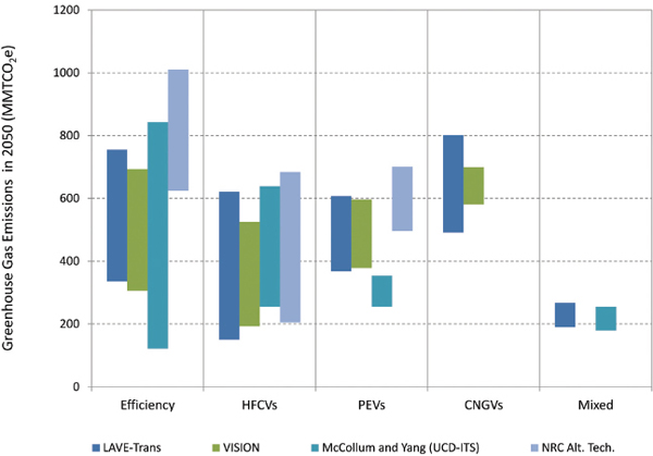
FIGURE 5.30 Comparison of greenhouse gas emissions scenarios.
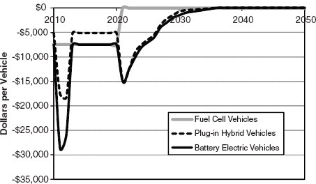
FIGURE 5.31 Assumed battery electric vehicle and plug-in hybrid electric vehicle subsidies in Optimistic EV Technology Scenario.
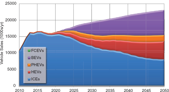
FIGURE 5.32 Vehicle sales by technology: Optimistic Plug-in Electric Vehicle Scenario.
random walk14 (e.g., Hamilton, 2009; Anderson et al., 2011; Alquist et al., 2012). And as emphasized above, many of the parameters that drive the committee’s modeling results are uncertain because knowledge of consumers’ evaluation of limited-range vehicles, limited fuel availability, and other key factors is poor for present circumstances and worse for 30 to 40 years in the future. And, of course, the future will present opportunities and challenges that were not anticipated. Vehicle Sales In this section, the LAVE model is used to illustrate some of the challenges these uncertainties present to policy makers.
Policies that would work well if technologies advance as in the committee’s midrange or optimistic cases may fail if technological progress stalls or is more expensive than anticipated. One technology may be expected to advance rapidly and yet a different technology turns out to exceed expectations. To illustrate these points, the LAVE model was used to construct three hypothetical scenarios. These scenarios are not predictions, nor do they reflect the committee’s Sales by Vehicle Technology judgments about the likelihood of success of the technologies used to illustrate the role of uncertainty. The choice of technologies that succeed or fail in the scenarios below is arbitrary.
The first scenario includes a policy of subsidies for PHEVs and BEVs that works well assuming optimistic technological progress for these two technologies and midrange progress for all others. The scenario also assumes high biofuel intensity and low-carbon production of electricity and hydrogen. The vehicle subsidies for 2010-2012 were chosen to match actual sales of BEV and PHEV vehicles in the United States and include the federal tax credit of $7,500 per vehicle, as well as state subsidies and implicit subsidies by manufacturers introducing these vehicles. Only the federal subsidy is assumed to continue until 2020 and then end. In 2021 a new subsidy of $15,000 per vehicle is assumed for
_______________________
14A random walk is a mathematical formalism for a stochastic process defined as a series of random steps. In this case, oil prices are considered as a Gaussian random walk, meaning that the size of the step follows a Gaussian probability distribution.
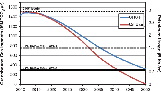
FIGURE 5.33 Changes in petroleum use and greenhouse gas emissions versus 2005: Optimistic Plug-in Electric Vehicle Scenario.
both vehicle types, decreasing each year until all subsidies are ended after 2035 (Figure 5.31).
The result is a successful, sustainable market penetration of PEVs. In 2050 BEVs attain a market share of 33 percent, PHEVs have an 8 percent share, and largely biofuel-powered HEVs and ICEVs claim 24 and 35 percent of the new-vehicle market, respectively (Figure 5.32).
The improvements in fuel economy, high penetration of drop-in biofuels (45 billion gallons in 2050), and market success of grid-connected vehicles powered by electricity produced by a low-carbon grid essentially eliminate oil use by LDVs and reduce GHG emissions by 78 percent, for all practical purposes meeting both 2050 goals. The 2030 goal is almost met by a 41 percent reduction in petroleum use versus the 2005 level (Figure 5.33).
The cost of subsidies to induce the transition is substantial, $130 billion NPV discounted to 2010 at 2.3 percent per year. The subsidies together with the lower energy costs of plug-in vehicles generate consumers’ surplus benefits that exceed the subsidy costs (Figure 5.34). When uncounted energy savings over the full life of the vehicles and the societal values of reduced GHG emissions and oil use are added to the other costs and benefits, the NPV of the transition policies is over $600 billion. The subsidies must be paid before most of the benefits are received, however, putting a large amount of capital at risk.
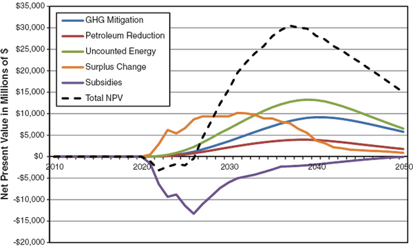
FIGURE 5.34 Net present value of the costs and benefits of the transition: Optimistic Plug-in Electric Vehicle Scenario.
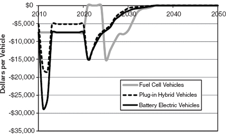
FIGURE 5.35 Assumed battery electric and plug-in hybrid electric vehicle subsidies in Pessimistic Plug-in Electric Vehicle Technology Scenario with Adaptation.
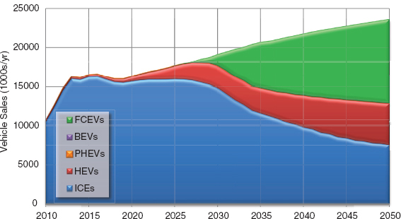
FIGURE 5.36 Vehicle sales by vehicle technology in Pessimistic Plug-in Electric Vehicle Technology Scenario with Adaptation.
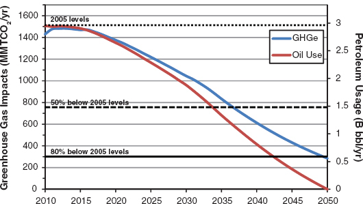
FIGURE 5.37 Changes in petroleum use and greenhouse gas emissions versus 2005 in Pessimistic Plug-in Electric Vehicle Technology Scenario with Adaptation to promote hydrogen fuel cell vehicles after 2024.
If the extreme assumption is made that the two technologies do not progress beyond their status today (BAU assumptions), the same subsidies that induced a sustainable transition in other cases are unsuccessful in achieving any sustainable market penetration. However, far less is spent on subsidies in this pessimistic PEV technology scenario, since the vehicles remain too expensive to attract many buyers. The total expenditures on the unsuccessful attempt to induce a transition amount to somewhat more than $1 billion. Costs exceed benefits, however, and the NPV of the scenario is on the order of –$250 million. Not surprisingly, the goals are not met in 2050, but petroleum use is still 75 percent lower than in 2005 and GHG emissions are 60 percent lower due to the much greater energy efficiency of ICEVs and HEVs and the extensive use of drop-in biofuels.
Suppose that the hypothetical failure of PEV technology to advance is quickly recognized, and that it is observed that FCEV technology is advancing more rapidly than expected. Further, assume that a decision is made to change course 3 to 4 years after the higher PEV subsidies are offered in 2021. Two hundred subsidized hydrogen refueling stations are built in 2024 followed by another 200 in 2025. Subsidies nearly identical to those previously offered for the plug-in vehicles are offered for FCEVs (Figure 5.35). Because it is assumed that the FCEV technology has progressed according to the midrange assumptions, this policy adaptation succeeds, resulting in nearly a 50 percent FCEV market share by 2050 (Figure 5.36). As a consequence, the 2050 goals for both oil and GHG reduction are met (Figure 5.37).
These scenarios are intended to illustrate the importance of uncertainty about future technology evolution and the value of adapting policies to the progress of technology. The choice of technologies for the illustration is entirely arbitrary. Which technology will succeed, if any, is uncertain. There will be costs to attempting to deploy technologies that do not progress to commercial competitiveness. However, if competitive alternatives emerge, and policies can be changed, it may still be possible to meet the long-term goals at a reasonable cost.
5.7 SIMULATING UNCERTAINTY ABOUT THE MARKET’S RESPONSE
In addition to uncertainty about the progress of alternative fuel and vehicle technologies (e.g., Bastani et al., 2012), there is also considerable uncertainty about how the market will respond to novel technologies. Many of the most important determinants of the market success of advanced technologies are poorly understood. These include the inconvenience cost of limited fuel availability for hydrogen and CNG, and limited range and long recharging times for BEVs. The number of innovators willing to pay a premium for novel technologies is largely unknown, as is the amount they would be willing to pay to get one of the first plug-in hybrid electric or hydrogen fuel cell vehicles. And while there are many estimates of consumers’ willingness to pay for fuel economy, there is at present no consensus on the subject (Greene, 2010). There are dozens of studies providing estimates of the sensitivity of consumers’ vehicle choices to price, yet little is known about the price sensitivity of choices among novel technologies. On the vehicle and fuels supply side, there is a great deal of uncertainty about learning rates, scale economies, and firms’ aversion to risk. Furthermore, all these factors can and likely will change over a 40-year period.
It is possible to get a sense of how these uncertainties affect the committee’s modeling results by means of simulation analysis. Table 5.6 lists 17 factors that determine market behavior in the LAVE model and provides mean values used in the model runs as well as uncertainty ranges based solely on the committee’s judgment. Ten thousand simulations of the LAVE model were run to produce distributions for key model outputs, including the impacts on GHG emissions and
TABLE 5.6 Model Parameters Included in Simulation Analysis and Ranges of Values
| Parameters | Distribution | Minimum | Mean | Maximum | |||||
| Importance of diversity of makes and models to chose from | Triangle | 0.50 | 0.67 | 0.9975932 | |||||
| Value of time ($/hr) | Triangle | $10.00 | $20.00 | $39.86 | |||||
| Maximum value of public recharging to typical PHEV buyer | Uniform | $500 | $1,000 | $1,500 | |||||
| Cost of 1 day on which driving exceeds BEV range | Uniform | $10,002 | $20,000 | $29,999 | |||||
| Maximum value of public recharging to typical BEV buyer | Uniform | $0 | $500 | $1,000 | |||||
| Importance of fuel availability relative to standard assumption | Triangle | 0.67 | 1.00 | 1.67 | |||||
| Payback period for fuel costs (yr) | Triangle | 2.0 | 3.0 | 5.0 | |||||
| Volume threshold for introduction of new models relative to standard assumptions | Uniform | 0.80 | 1.00 | 1.20 | |||||
| Optimal production scale relative to standard assumptions | Uniform | 0.75 | 1.00 | 1.25 | |||||
| Scale elasticity relative to standard assumptions | Uniform | 0.50 | 1.00 | 1.50 | |||||
| Progress ratio relative to standard assumptions | Uniform | 0.96 | 1.00 | 1.04 | |||||
| Price elasticities of vehicle choice relative to standard assumptions | Uniform | 0.60 | 1.20 | 1.80 | |||||
| Percentage of new car buyers who are innovators | Triangle | 5.0 | 15.0 | 20.0 | |||||
| Willingness of innovators to pay for novel technology ($/mo) | Uniform | $100 | $200 | $300 | |||||
| Cumulative production at which innovators’ willingness to pay is reduced by half | Uniform | 1,000,000 | 2,000,000 | 3,000,000 | |||||
| Majority’s aversion to risk of new technology ($/mo) | Uniform | −$900 | −$600 | −$300 | |||||
| Cumulative production at which majority’s risk is reduced by half | Uniform | $500,000 | $1,000,000 | $1,500,000 | |||||
petroleum consumption, and the market shares of advanced vehicle technologies. Not all elements of market uncertainty are included in the simulations. In particular, the LAVE model does not include a representation of industry’s likely aversion to risky investments. Nor do the simulation runs include uncertainty about future energy prices.
Two scenarios were simulated: policies to induce a transition to PEVs and policies to induce a transition to FCEVs. Both scenarios include 13.5 billion gallons of drop-in biofuel by 2050 and 10 billion gallons gasoline equivalent of ethanol, as well as the energy efficiency improvements of the midrange scenario.
The resulting uncertainty is strikingly large. The simulated distribution of GHG emissions reductions for the FCEV Policy Case ranges from 43 percent, corresponding to zero market penetration of fuel cell vehicles, to 83 percent at a 60 percent market share of FCEVs (Figure 5.38). It is bi-modal, reflecting the presence of tipping points that cause FCEVs to succeed to a greater or lesser degree, or fail to achieve any significant market share. The existence of tipping points reflects the many positive feedbacks in the transition process. The simulated distribution of greenhouse gas reductions due to plug-in vehicles has a similar bi-modal form and nearly as great a range: –42 to –71 percent (Figure 5.39). The modal separation is less because EVs do not have the strong dependence on fuel availability that hydrogen vehicles do.
The impacts are highly uncertain chiefly because the market response to electric-drive technology is uncertain. The simulated distribution of BEVs’ share of the new LDV market in 2050 is shown in Figure 5.40. Although there is a peak in the vicinity of 30 percent, there is a reasonable probability of almost any market share between zero and 50 percent, and a nearly 30 percent probability of almost no market share. The situation for FCEVs is similar but there is a greater separation between market success and failure (Figure 5.41). The simulation analysis can also identify those parameters that have the greatest influence on market success. Both technologies are highly sensitive to assumptions about scale economies in the automotive industry, to the number of innovators and their willingness to pay for novel technology, and to the value to consumers of having a diverse array of vehicles to choose from. BEVs do better if consumers are more sensitive to energy costs and less sensitive to initial price. Consumers’ concern about range and recharging-time limitations is also very important for BEVs. Fuel cell vehicles’ market success is strongly dependent on the importance of fuel availability, but this factor is of much less importance for BEVs.
There are many reasons that these results should be interpreted cautiously, not the least of which is that a fixed policy strategy is assumed, regardless of the parameter values chosen. As is the case for uncertainty about technological progress, adapting policies to suit the realities of the marketplace would undoubtedly produce better results. All of the frequency distributions shown are conditional on a set of specific policy assumptions that are held constant for all simulations.
The uncertainties illustrated here can be reduced by research and analysis, and by learning from experience. Clearly, there is a great deal of benefit to be gained from a better understanding of both the technologies and the behavior of the market. Uncertainty analysis does not describe the future as it must be or as it will be; it is an attempt to describe
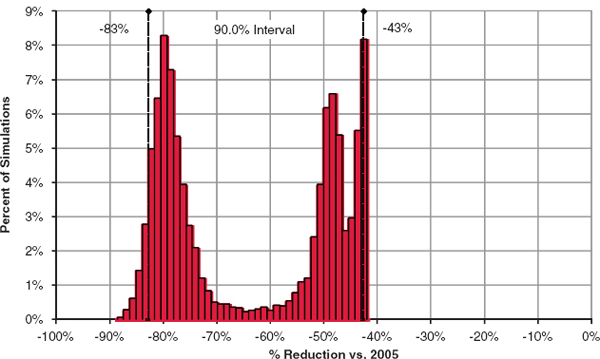
FIGURE 5.38 Distribution of estimated greenhouse gas emissions reductions from 2005 level: Fuel Cell Electric Vehicles Case.
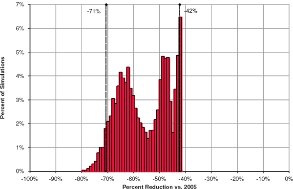
FIGURE 5.39 Distribution of estimated greenhouse gas reduction in 2050 from 2005 level: Plug-in Electric Vehicles.
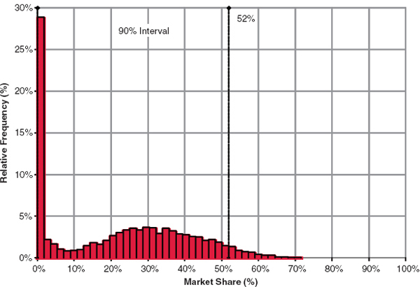
FIGURE 5.40 Distribution of battery electric vehicle market share in 2050: Plug-in EV Policy Case.
what we think we do and do not know about the distant future, as viewed from the present. Learning—increasing knowledge of the processes and behaviors that will affect a transition, as well as the costs and performance of the technologies that could enable one—is likely to be essential if the 2030 and 2050 goals are to be achieved efficiently. Inducing a transition to non-petroleum energy sources with extremely low GHG emissions is an unprecedented challenge for public policy. To support effective policy making, a much better understanding of how markets and technology will interact is likely to be highly beneficial.
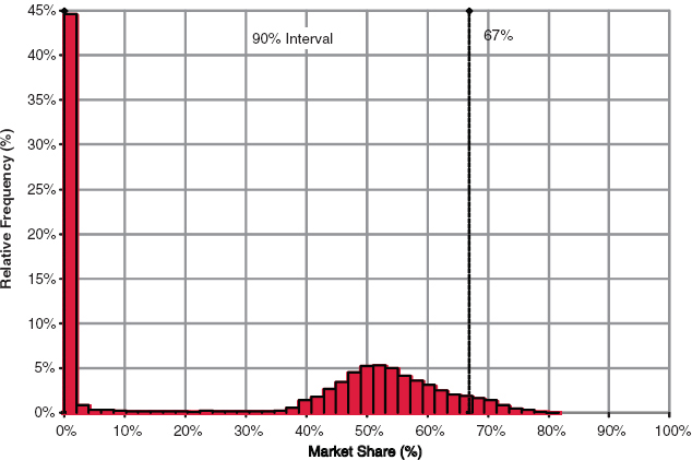
FIGURE 5.41 Distribution of hydrogen fuel cell vehicle market share in 2050: Fuel Cell Electric Vehicle Policy Case.
Large and important reductions in petroleum use and greenhouse gas emissions can be achieved by increasing the fuel economy of light-duty vehicles in line with the CAFE standards for 2025 and embodied in the RFS2 (25-30 percent by 2030 and 30-40 percent by 2050). Even greater reductions will be possible if advances in vehicle and fuel technologies beyond those required to meet the 2025 CAFE standards and the RFS2 standards can be realized.
Achieving the 2030 and 2050 goals for reduction of oil use and greenhouse gas emissions will require a mix of strong public policies, market forces that encourage greater energy efficiency, and continued improvements in vehicle and fuels technologies. As the comparison of VISION and LAVE-Trans model estimates illustrates, reaching the goals is likely to be more difficult than previous “what if” analyses have concluded due to economic feedback effects and competition among technologies and fuels. These feedback effects include increased vehicle use with reduced energy costs, increased new-vehicle demand with improved technology, and competition for market share among advanced technologies. They are also almost certain to include lower petroleum prices as a consequence of reduced petroleum demand, although no attempt has been made to model that in these analyses. These feedback effects are much smaller in magnitude than the direct effects of energy efficiency improvement and displacement of petroleum with alternative energy sources; still, they increase the difficulty of achieving the 2050 goals.
Achieving a 40 percent reduction in petroleum use over 2005 levels by 2030 is a more realistic and achievable goal than a 50 percent reduction. Whether or not this level of reduction would be sufficient to achieve the objective of solving the nation’s oil dependence problem given expected increases in domestic petroleum supply should be carefully evaluated.
Even if the nation should fall short of the 2050 goals, there are likely to be environmental, economic, and national security benefits resulting from the reductions that are achieved. The committee’s modeling suggests that reductions in petroleum use on the order of 70 to 90 percent are possible given very strong policies and continued advances in the key technologies: electric-drive vehicles (hybrid, plug-in hybrid, battery, and fuel cell) and drop-in biofuels. In the committee’s judgment, reductions in greenhouse gas emissions on the order of 60 to 80 percent are possible but will require effective and adaptive policies over time as well as continued advances in the technologies described in Chapters 2 and 3.
Including the social costs of GHG emissions and petroleum dependence in the cost of fuels (e.g., via a carbon tax) provides important signals to the market that will promote technological development and behavioral changes. Yet these pricing strategies alone are likely to be insufficient to induce a major transition to alternative, net-low-carbon vehicle technologies and/or energy sources. Additional strong, temporary policies may be required to break the lock-in of conventional technology and overcome the market barriers to alternative vehicles and fuels.
If two or more of the fuel and/or vehicle technologies evolve through policy and technology development as shown in a number of the committee’s scenarios, the committee’s model calculations indicate benefits of making a transition to a low-petroleum, low-GHG energy system for LDVs that exceed the costs by a wide margin. Benefits include energy cost savings, improved vehicle technologies, and reductions in petroleum use and GHG emissions. Costs refer to the additional costs of the transition over and above what the market is willing to do voluntarily. However, as noted above, modeling results should be viewed as approximations at best because there is by necessity in such predictions a great deal of uncertainty in estimates of both benefits and costs. Furthermore, the costs are likely to be very large early on with benefits occurring much later in time.
Depending on the readiness of technology and the timing of policy initiatives, subsidies or regulations for new vehicle energy efficiency and the provision of energy infrastructure may be required, especially in the case of a transition to a new vehicle and fuel system. In such cases, substantial subsidies might be required for at least 5 to 10 years, and possibly as long as 20 years if technological progress is slow (e.g., starting grid-connected vehicles now is likely to require 20 years of subsidy to stabilize them at a significant market share). And, as shown above, there is likely to be a high degree of risk in policies targeted to a particular technology. For these reasons, it is important to consider carefully when and if such policies are necessary and to make policy adaptable to changing evidence about technology and market conditions. It is also very important that policy makers obtain objective, expert advice on the readiness of both fuel and vehicle technologies and markets. Scenario analysis has identified strong tipping points for the transition to new vehicle technologies. If sufficiently large subsidies are not applied to overcome the early cost differentials, then the transition will not occur and the subsidies will have been wasted. In pursuing these goals, the rate of cost decline and the subsidies applied at each stage must be carefully weighed to establish that the program is effective.
Advance placement of refueling infrastructure is critical to the market acceptance of hydrogen fuel cell and CNG vehicles. It is likely to be less critical to the market acceptance of grid-connected vehicles, since many consumers will have the option of home recharging. However, the absence of an outside-the-home refueling infrastructure for grid-connected vehicles is likely to depress demand for these vehicles. Infrastructure changes will not be needed if the most cost-effective solution evolves in the direction of more efficient ICEVs and HEVs combined with drop-in low-carbon biofuels.
Empirical knowledge of the barriers to major energy transitions is currently inadequate to make robust assessments of public policies. The modeling analysis presented in this chapter is intended to be an initial step in the right direction rather than a definitive assessment of alternatives. Research is needed to better understand key factors for transitions to new vehicle fuel systems such as the costs of limited fuel availability, the disutility of vehicles with short ranges and long recharge times, the numbers of innovators and early adopters among the car-buying public, as well as their willingness to pay for novel technologies and the risk aversion of the majority, and much more. More information is also need on the transition costs and barriers to production of alternative drop-in fuels, especially on the type of incentives necessary for biofuels. The models that the committee and others have used to analyze the transition to alternative vehicles and/or fuels are first-generation efforts, more useful for understanding processes and their interactions than producing definitive results.
Alquist, R., L. Kilian, and R.J. Vigfusson. 2012. Forecasting the price of oil. In Handbook of Economic Forecasting, Volume 2 (G. Elliott and A. Timmermann, eds.). Amsterdam: Elsevier-North-Holland.
Anderson, S.T., R. Kellogg, and J.M. Sallee. 2011. What Do Consumers Believe about Future Gasoline Prices? Working Paper 16974. National Bureau of Economic Research Working Paper Series. Cambridge, Mass.: National Bureau of Economic Research. April.
ANL (Argonne National Laboratory). 2009. Multi-Path Transportation Futures Study: Vehicle Characterization and Scenario Analyses. ANL/ESD/09-5. Prepared for the U.S. Department of Energy. Argonne, Ill.: Energy Systems Division, Argonne National Laboratory. July.
———. 2011. Light-Duty Vehicle Fuel Consumption Displacement Potential Up to 2045. ANL/ESD/11-4. Argonne, Ill.: Energy Systems Division, Argonne National Laboratory. July.
Bandivadekar, A., K. Bodek, L. Cheah, C. Evans, T. Groode, J. Heywood, E. Kasseris, M. Kromer, and M. Weiss. 2008. On the Road in 2035: Reducing Transportation’s Petroleum Consumption and GHG Emissions. Laboratory for Energy and the Environment Report No. LFEE 2008-05 RP. Cambridge, Mass.: Massachusetts Institute of Technology. July.
Bastani, P., J.B. Heywood, and C. Hope. 2012. The effect of uncertainty on U.S. transport-related GHG emissions and fuel consumption out to 2050. Transportation Research, Part A: Policy and Practice 46(3):517-548.
Boardman, A.E., D.H. Greenberg, A.R. Vining, and D.L. Weimer. 2011. Cost-Benefit Analysis: Concepts and Practice. Fourth Edition. Upper Saddle River, N.J.: Prentice Hall.
Brown, S.P.A., and H.G. Huntington. 2010. Reassessing the Oil Security Premium. Discussion Paper RFF DP 10-05. Washington, D.C.: Resources for the Future.
Copulos, M.R., 2003. America’s Achilles Heel: The Hidden Costs of Imported Oil. Washington, D.C.: National Defense Council Foundation.
Daly, A., and S. Zachary. 1979. Improved multiple choice models. In Identifying and Measuring Transportation Mode Choice (D. Hensher and Q. Dalvi, eds.). London: Teakfield.
Delucchi, M.A., and J.J. Murphy. 2008. US military expenditures to protect the use of Persian Gulf oil for motor vehicles. Energy Policy 36:2253-2264.
DOE (U.S. Department of Energy). 2011. U.S. Billion Ton Update: Biomass Supply for a Bioenergy and Bioproducts Industry. R.D. Perlack and B.J. Stokes, Leads. ORNL/TM-2011/224. Oak Ridge, Tenn.: Oak Ridge National Laboratory. August.
DOT (U.S. Department of Transportation). 2010. Transportation’s Role in Reducing U.S. Greenhouse Gas Emissions. Prepared by the U.S. DOT Center for Climate Change and Environmental Forecasting, Washington, D.C. April.
EIA (Energy Information Administration). 2011a. Annual Energy Outlook 2011. DOE/EIA-0383(2011). Washington, D.C.: Department of Energy, Energy Information Administration. March.
———. 2011b. Annual Energy Review 2010. DOE/EIA-0384(2010). Washington, D.C.: Department of Energy, Energy Information Administration. October.
———. 2012. Annual Energy Outlook 2012. DOE/EIA-0383ER(2012). Washington, D.C.: Department of Energy, Energy Information Administration. Available at http://www.eia.gov/forecasts/aeo/er/.
EPA and NHTSA (U.S. Environmental Protection Agency and National Highway Transportation Safety Administration). 2011. Draft Joint Technical Support Document: Proposed Rulemaking for 2017-2025 Light-Duty Vehicle Greenhouse Gas Emission Standards and Corporate Average Fuel Economy Standards. EPA-420-D-11-901. Washington, D.C. November.
EPRI (Electric Power Research Institute) and NRDC (Natural Resource Defense Council). 2007. Environmental Assessment of Plug-In Hybrid Electric Vehicles. Volume 1: Nationwide Greenhouse Gas Emissions. Palo Alto, Calif.: EPRI. July.
GAO (U.S. Government Accountability Office). 2006. Strategic Petroleum Reserve: Available Oil Can Provide Significant Benefits, But Many Factors Should Influence Future Decisions About Fill, Use and Expansion. GAO-06-872. Washington, D.C.: GAO. August.
Greene, D.L. 2009. Measuring energy security: Can the United States achieve oil independence? Energy Policy 38(4):1614-1621.
———. 2010. How Consumers Value Fuel Economy: A Literature Review. EPA-420-R-10-008. Washington, D.C.: U.S. Environmental Protection Agency.
Greene, D.L., and P.N. Leiby. 1993. The Social Costs to the U.S. of Monopolization of the World Oil Market, 1972-1991. ORNL-6744. Oak Ridge, Tenn.: Oak Ridge National Laboratory. March.
———. 2007. Integrated Analysis of Market Transformation Scenarios with HyTrans. ORNL/TM-2007/094. Oak Ridge, Tenn.: Oak Ridge National Laboratory. June.
Greene, D.L., and S.E. Plotkin. 2011. Reducing Greenhouse Gas Emissions from U.S. Transportation. Prepared for the Pew Center on Global Climate Change. Arlington, Va. January.
Greene, D.L., P.D. Patterson, M. Singh, and J. Li. 2005. Feebates, rebates and gas-guzzler taxes: A study of incentives for increased fuel economy. Energy Policy 33(6):757-775.
Hamilton, J.D. 2009. Understanding crude oil prices. The Energy Journal 30(2):179-206.
Huntington, H.G. 2007. Oil Shocks and Real U.S. Income. The Energy Journal 28(4):31-46.
Interagency Working Group on Social Cost of Carbon. 2010. Technical Support Document: Social Cost of Carbon for Regulatory Impact Analysis Under Executive Order 12866. Washington, D.C. February.
Jones, D.W., P.N. Leiby, and I.K. Paik, 2004. Oil price shocks and the macroeconomy: What has been learned since 1996? The Energy Journal 25(2):1-32.
Kaufmann, W.W., and J.D. Steinbruner, 1991. Decisions for Defense: Prospects for a New Order. Washington, D.C.: Brookings Institution. April.
Leiby, P.N. 2008. Estimating the Energy Security Benefits of Reduced U.S. Oil Imports, Final Report. ORNL/TM-2007/028. Oak Ridge, Tenn.: Oak Ridge National Laboratory, Revised March 14.
McCollum, D.L., and C. Yang. 2009. Achieving deep reductions in U.S. transport greenhouse gas emissions: Scenario analysis and policy implications. Energy Policy 37(12):5580-5596.
McConnell, J.M., 2008. Annual Threat Assessment of the Director of National Intelligence for the Senate Select Committee on Intelligence. SSCI ATA FEB 2008-DNI. Unclassified Statement for the Record. Washington, D.C.: Office of the Director of National Intelligence. February 5.
McFadden, D.L. 1978. Modeling the choice of residential location. In Spatial Interaction Theory and Planning Models (A. Karlqvist, L. Lundqvist, F. Snickars, and J. Weibull, eds.). Amsterdam: North Holland.
Military Advisory Board, 2011. Ensuring America’s Freedom of Movement: A National Security Imperative to Reduce Oil Dependence. Alexandria, Va.: Center for Naval Analyses.
Moreland, H., 1985. A Few Billion for Defense Plus $250 Billion for Overseas Military Intervention. New Policy Papers #1. Washington, D.C.: Coalition for a New Foreign and Military Policy.
NRC (National Research Council). 2008. Transitions to Alternative Transportation Technologies: A Focus on Hydrogen. Washington, D.C.: The National Academies Press.
———. 2009a. Hidden Costs of Energy: Unpriced Consequences of Energy Production and Use. Washington, D.C.: The National Academies Press.
———. 2009b. America’s Energy Future: Liquid Transportation Fuels from Coal and Biomass. Washington, D.C.: The National Academies Press.
———. 2010a. Transitions to Alternative Transportation Technologies: Plug-in Hybrid Electric Vehicles. Washington, D.C.: The National Academies Press.
———. 2010b. America’s Energy Future: Real Prospects for Energy Efficiency in the United States. Washington, D.C.: The National Academies Press.
OMB (Office of Management and Budget). 2012. Appendix C: Discount Rates for Cost-Effectiveness, Lease, Purchase, and Related Analyses. OMB Circular No A-94. Memorandum from the Executive Office of the President of the United States. Washington, D.C. January 3.
Pacala, S., and R. Socolow. 2004. Stabilization wedges: Solving the climate problem for the next 50 years with current technologies. Science 305(5686):968-972.
Parry, I.W.H., and J. Darmstadter. 2004. The Costs of US Oil Dependency. Washington, D.C.: Resources for the Future. November 17.
Ravenal, E.C. 1991. Designing Defense for a New World Order: The Military Budget in 1992 and Beyond. Washington, D.C.: Cato Institute.
Singh, M., A. Vyas, and E. Steiner. 2003. VISION Model: Description of Model Used to Estimate the Impact of Highway Vehicle Technologies and Fuels on Energy Use and Carbon Emissions to 2050. Prepared by Argonne National Laboratory for the Department of Energy under Contract No. W-31-109-ENG-38. Report#ANL-ESD-04-1. Argonne, Ill.: Argonne National Laboratory. December.
UCD (University of California, Davis). 2011. Sustainable Transportation Energy Pathways: A Research Summary for Decision Makers (J. Ogden and L. Anderson, eds.). Davis, Calif.: Institute of Transportation Studies.
Vyas, A.D., D.J. Santini, and L.R. Johnson. 2009. Potential of plug-in hybrid electric vehicles’ to reduce petroleum use: Issues involved in developing reliable estimates. Journal of the Transportation Research Board 2139:55-63.
Williams, H.C.W.L. 1977. On the formation of travel demand models and economic measures of user benefit. Pp. 285-344 in Environment and Planning, Part A, Volume 9. London: Pion, Ltd.
Yeh, S., A.E. Farrell, R.J. Plevin, A. Sanstad, and J. Weyant. 2008. Optimizing U.S. mitigation strategies for the light-duty transportation sector: What we learn from a bottom-up model. Environmental Science and Technology 42(22):8202-8210.


