
1
The Growing Problem of Nonresponse
The problem of nonresponse in social science surveys in the United States has been succinctly summarized by the sponsor of this study, the Russell Sage Foundation (2010), in a foreword to the foundation’s description of this study:
Household survey responses rates in the United States have been steadily declining for at least the last two decades. A similar decline in survey response can be observed in all wealthy countries, and is particularly high in areas with large numbers of single-parent households, families with young children, workers with long commutes, and high crime rates. Efforts to raise response rates have used monetary incentives or repetitive attempts to obtain completed interviews, but these strategies increase the costs of surveys and are often unsuccessful. Why is response declining and how does it increase the possibility of inaccurate survey results? Most important, with the advancement of reliable social science research at stake, what are effective methods for increasing the response rate for household surveys?
In examining the extent and effect of nonresponse in social science surveys and the steps that can be taken to reduce the effects of nonresponse, an overriding concern is that the validity of social science studies and their conclusions is indeed at stake. Apparent trends in nonresponse, if not arrested, are likely to weaken the validity of inferences drawn from estimates based on household surveys and undermine, perhaps fatally, their potential to elicit information that assists in understanding social and economic issues. There has always been incomplete acceptance that social science is science. Doubts about the validity of data from surveys give ammunition
to critics of social science and other skeptics reluctant to accept the conclusions of social scientific investigations.
Moreover, these trends undermine researchers’ (and the public’s) confidence in the use of the survey as a tool in the development of public policy responses to social problems. This growing lack of confidence stands in stark contrast to the recent trends of very rapid growth in the use of surveys in social science and in the variety of methods used to conduct surveys. In documenting trends in government-sponsored social science survey research over a recent two-decade span, Presser and McCulloch (2011) found that the number of surveys increased by more than 50 percent over the period 1984 to 2004 and that the number of respondents approved for studies cleared by the Office of Management and Budget (OMB) increased by more than 300 percent. The authors point out that the relative increase in the number of surveys was many times greater than the relative increase in the size of the general population during the same time frame.
The modes employed by surveys in the public and private sectors have proliferated as new technologies and methodologies have emerged, but each of these new technologies and processes has its own set of methodological issues and its own nonresponse profile. To the traditional trio of mail, telephone, and face-to-face surveys, researchers have added interactive voice response (IVR), audio computer-assisted self-interviewing (ACASI), and Web surveys. In addition, new methods of sampling (such as address-based sampling) have emerged. The proliferation of modes of data collection has been accompanied by a growing public and private research agenda focused on seeking solutions to aspects of the problem of survey nonresponse, ranging from better training and deployment of interviewers, to increased use of incentives, to better use of information collected during the survey process, and to increased use of auxiliary information from other sources in survey design and estimation.
In this chapter, we set the stage for subsequent discussions of the issues surrounding survey nonresponse, its consequences, and proposed approaches to these issues by examining the nature and extent of nonresponse in social science surveys. We lay out evidence regarding the trends in nonresponse rates overall and by survey mode, and we consider evidence that increasing levels of nonresponse are an international phenomenon. We also explore some of the reasons for growing nonresponse rates. Finally, we discuss the current state of knowledge about some of the practical implications of growing nonresponse rates for survey costs and survey management. The evidence presented in this chapter leads to several recommendations for a research agenda aimed at filling some of the current gaps in our knowledge concerning trends in nonresponse as well as the reasons for those trends.
CONCEPTUALIZING AND DEFINING NONRESPONSE
Great strides have been made over the past three decades in conceptualizing and defining survey nonresponse, and this work has led to a growing consensus about the root causes and the definition and classification of types of survey nonresponse—a necessary first step in the development of metrics about nonresponse and in coming to grips with the consequences.
The decision of a person whether to respond to a survey involves several key factors, and an examination of those factors can be laid out as a conceptual framework for considering survey nonresponse issues. The elaboration of these factors provides a convenient conceptual point of departure for this review.
A main, overriding factor is a cost-benefit analysis: People respond to surveys when they conclude that the rewards outweigh the costs. Societal factors also enter in. If there is social disorganization or high crime rates, for example, some respondents will be more likely to refuse. There may be differences in the likelihood to respond among different sociodemographic groups, with some more or less prone to take part in surveys. The survey setting also may influence the decision to respond—which in most cases, particularly in a telephone environment, may be a near-instantaneous decision—and interviewers play a key role in determining cooperation, especially in face-to-face surveys. In the larger sense, a growing societal concern over intrusions on people’s time and privacy may have an influence. Attitudes also play a part. The growth in the number of surveys has led to stronger attitudes about surveys in general, apart from attitudes about the topic. The salience of the topic plays a role, and participation may be partly an emotional decision. The mode of data collection may also affect response propensities. And finally, there may be a random component to the decision whether or not to cooperate. These factors are each explored in some depth in this report.1
The advances made toward arriving at a definitional consensus on nonresponse have been largely the result of ongoing work by the American Association for Public Opinion Research (AAPOR), which in the late 1990s began publication of its Standard Definitions: Final Dispositions of Case Codes and Outcome Rates for Surveys. This volume has been subsequently amended and updated, most recently in 2011.2
The survey research community has, under the leadership of AAPOR,
______________________________________
1The conceptual framework that is presented here was drawn largely from the survey methodology field, with the understanding that every field of social science has concepts and frameworks that might shed light on the problem of growing nonresponse, its causes, and its consequences.
2The AAPOR work in this field was preceded by a project to develop standard definitions by the Council of American Survey Research Organizations.
focused on four operational definitions of rates of survey participation: cooperation rates, contact rates, refusal rates, and response rates. These definitions differ in more than nuance. According to the definitions in the AAPOR Standard Definitions volume referred to above, cooperation rates are the proportion of all cases interviewed of all eligible units ever contacted; contact rates are the proportion of all cases in which some household member was actually reached; refusal rates are the proportion of all potentially eligible cases in which the housing unit or the sample member refuses to be interviewed or breaks off the interview;3 and the most familiar rate, the response rate, represents the proportion of complete interviews, with responding units divided by the number of eligible units in the sample (American Association for Public Opinion Research, 2011). In view of the importance of response rate as a descriptor of the quality of a survey, AAPOR provides six related formulas for calculating response rates (see Box 1-1) and also defines different measures for different modes of survey collection.
There is now general concurrence with the overall AAPOR framework throughout the social science survey community. Indeed, several journals now require that one of the AAPOR response rates be reported when survey results are presented. Even with the rich variety of AAPOR definitions, however, some survey organizations have had to supplement these definitions with ancillary concepts and definitions based on their own needs and buttressed by their own research. Yet, by and large, the definitions have leveled the playing field and have held up well, except in one case: The distinction between contact and cooperation rates has been a source of confusion for some. Calculating household-level contact and cooperation rates requires obtaining information on contact or lack of contact with the household. The distinctions between them are often blurred, and in an era when more and more people are taking steps to limit their accessibility, research is needed on whether the distinction between contact and cooperation is still useful to maintain.
Recommendation 1-1: Research is needed on the different factors affecting contact and cooperation rates.
The process of reaching a consensus definition of nonresponse rates is illustrated by the process within the federal government, which spon-
______________________________________
3Break-offs may occur at several points in the interview. As a rule of thumb, an interview is considered a break-off refusal when less than 50 percent of applicable questions are answered; those with 50–80 percent answered are considered partial responses; and those with 80 percent or more answered are considered completed responses (American Association for Public Opinion Research, 2011, p. 14).
BOX 1-1
What Is a Response Rate?
Response Rate 1 (RR1), or the minimum response rate, is the number of complete interviews divided by the number of interviews (complete plus partial) plus the number of non-interviews (refusal and break-off plus non-contacts plus others) plus all cases of unknown eligibility.
Response Rate 2 (RR2) counts partial interviews as respondents but otherwise is identical to RR1.
Response Rate 3 (RR3) estimates e, the proportion of cases with unknown eligibility that are actually eligible. In estimating e, researchers should be guided by the best available scientific information on what share eligible cases make up among the unknown cases and should not select a proportion in order to boost the response rate. The basis for the estimate must be explicitly stated and detailed.
Response Rate 4 (RR4) allocates cases of unknown eligibility as in RR3, but also includes partial interviews as respondents as in RR2.
Response Rate 5 (RR5) is either a special case of RR3 in that it assumes that e = 0 (i.e., that there are no eligible cases among the cases of unknown eligibility) or the rare case in which there are no cases of unknown eligibility.
Response Rate 6 (RR6) makes the same assumption as RR5 and also includes partial interviews as respondents. RR5 and RR6 are appropriate only when it is valid to assume that none of the unknown cases are eligible ones, or when there are no unknown cases. RR6 represents the maximum response rate.
SOURCE: Excerpted (without equations) from American Association for Public Opinion Research (2011, pp. 44–45).
sors and conducts some of the largest and most significant social science surveys in the United States. The federal government ventured into documenting and defining trends in unit nonresponse in reaction to studies conducted by the Federal Committee on Statistical Methodology (FCSM) in the 1990s (Johnson et al., 1994; Shettle et al., 1994). These studies found little consistency in how the federal surveys that they reviewed measured and reported nonresponse rates. These inconsistencies were found to have been due mainly to differences in sample design across the surveys. Still, as recently as 2000 it was observed that the official publication of many response rates from government surveys was “fragmented, sporadic, and non-standardized” (Bates et al., 2000). The lack of standardized reporting
of response rates for federal surveys was again documented in FCSM Working Paper 31 (Office of Management and Budget, 2001). The comparability issues are exacerbated for international comparisons where refusals are handled differently.
OMB has subsequently issued policy guidance to standardize nonresponse rate definitions and to set targets for acceptable survey response rates—no easy task since government surveys vary widely in their mandate, sample design, content, interview period, mode, respondent rules, and periodicity. The main source of this guidance is the OMB Statistical and Science Policy Office release titled Guidance on Agency Survey and Statistical Information Collections—Questions and Answers When Designing Surveys for Information Collections (Office of Management and Budget, 2006). This document provides information on the OMB clearance process for surveys and other statistical information collections. Included is information about defining response rates. In summary, the document encourages agencies to use the AAPOR standard formulas in calculating and reporting response rates in clearance submissions to OMB, while permitting agencies to “use other formulas as long as the method used to calculate response rates is documented” (Office of Management and Budget, 2006, p. 57).
The existing formal definitions of nonresponse rates take the outcome of a case, response or nonresponse, as given. Although there is relatively little ambiguity about what constitutes response, nonresponse may cover a broad range of possibilities beyond “refusal” and “no contact.” Some nonresponse may reflect refusals that are so adamant that conversion is a virtual impossibility, but in other cases there is a degree of judgment about the utility of following up, perhaps with another interviewer or a specialized refusal convertor in an interviewer-mediated survey. Respondents who are not contacted might not be reached because they are away for a prolonged period, because contact was poorly timed, or simply because contact is random and more attempts would have been needed. It is only relatively recently that it has become possible, with the use of electronic records to quantify attempts on individual cases, to make a broad exploration of effort and nonresponse. The availability of such electronic records opens the doors to new avenues of research, and additional work in this area is needed.
LONG-TERM TRENDS IN RESPONSE RATES
Evidence concerning trends in response rates in general population surveys has been accumulating for over three decades. In an early trend study, Steeh (1981) found that refusals were increasing in U.S. academic surveys conducted between 1952 and 1979. In 1989, Groves summarized the literature and concluded that “participation in social surveys by sample
households appears to be declining in the United States over time.” Later, in the early 1990s, the concern grew to a crescendo with new evidence offered by Bradburn (1992) that response rates were declining and had been declining for some time. It became apparent that this decline in response rates was becoming widespread. This concern was buttressed by the experience of the 1990 Census of Population and Housing, which saw an unexpected and significant decline in mailback responses (Fay et al., 1991). Brehm (1994) found that all sectors of the survey industry—academic, government, business, and media—were suffering from falling response rates. Groves and Couper (1998) likewise concluded that the decline in response rates was being experienced by government, academic, and commercial surveys. Their summary of data from other countries was based on surveys with long time series and found, for example, that while response to the Canadian Labor Force Survey appeared to be stable over the years, nonresponse appeared to be increasing in Holland, Japan, and Sweden. These repeated surveys are thought to be especially valuable indicators of time trends because their designs remain stable across years. Campanelli et al. (1997) also corroborated this trend, but they found that there were some surveys that had managed to maintain their response rates, although at the expense of a larger investment in time and money.
This direct evidence was accompanied by a growing literature exhibiting concern about the size and effects of nonresponse, evidenced by studies such as National Research Council (1983), Goyder (1987), Lessler and Kalsbeek (1992), Brehm (1993), Groves and Couper (1998), De Leuw and De Heer (2002), Groves et al. (2002), and Stoop (2005). In addition, the Journal of Official Statistics devoted special issues to nonresponse in 1999, 2006, and 2011. The most recent in this series evidenced the growing maturity in the field, emphasizing assessment of nonresponse bias and its impact on analysis (Blom and Kreuter, 2011).
In her introduction to the 2006 special edition of Public Opinion Quarterly, Singer (2006) cited multiple sources to support the consensus view that nonresponse rates in U.S. household surveys have increased over time. Although not discussed in this paper, household survey nonresponse is a matter of growing concern in many countries.4
______________________________________
4International comparative data on response rates and types of nonresponse in combination with data on design and collection strategies are scarce. While studies have shown that response rates differ across countries and over time, international data should be interpreted with caution. There are differences in survey design (such as mode of data collection and whether the survey is mandatory) and survey organization and implementation. Comparisons from the European Social Survey, a biennial face-to-face survey of attitudes, opinions, and beliefs in around 30 European countries, finds that, although the target response rate is 70 percent, in practice response rates are often lower and vary across countries (Stoop et al., 2010, p. 407). At our panel’s workshop, Lilli Japec of Statistics Sweden reported that nonresponse
Based on the above evidence, we are able to conclude that response rates continue on a long-term downward path, but we are concerned that solid evidence about the reasons for the decline is still elusive.
Recommendation 1-2: Research is needed to identify the person-level and societal variables responsible for the downward trend in response rates. These variables could include changes in technology and communication patterns, which are also reflected in changes in methods of collecting survey data.
Recommendation 1-3: Research is needed on people’s general attitudes toward surveys and on whether these have changed over time.
Recommendation 1-4: Research is needed about why people take part in surveys and the factors that motivate them to participate.
RESPONSE RATE TRENDS IN CROSS-SECTIONAL SURVEYS
This section reviews the recent experiences with response rates for several large and high-visibility repeated cross-sectional surveys. The surveys were selected to be illustrative of some of the more prominent surveys that produce information used in the social sciences. The discussion is abstracted from a paper prepared for this study by Brick and Williams (2013), who conducted an extensive literature review and examined four surveys from the late 1990s to the late 2000s. Two of them were face-to-face surveys—the National Health Interview Survey (NHIS) and the General Social Survey (GSS)—and two were list-assisted random digit dialing (RDD) telephone surveys—the National Household Education Survey (NHES) and the National Immunization Survey (NIS). We have added discussions of two additional telephone surveys: the Behavioral Risk Factor Surveillance System (BRFSS) and the Survey of Consumer Attitudes (SCA). We supplement the work of Brick and Williams with a discussion of results of analysis performed by the Census Bureau, the Bureau of Labor Statistics, and the Federal Reserve Board on response rates in the surveys they conduct.
______________________________________
in the Swedish Labor Force survey went from 2 percent to nearly 25 percent between 1963 and 2010. Among her findings were that response rates were higher when interviewers found the survey to be very interesting and among interviewers who had a positive attitude toward persuasion. At the sampled person level, there were lower response rates for non-Swedish citizens and persons 64 years of age and older and higher response rates for married persons.
National Health Interview Survey
The NHIS samples households as well as one adult and child within each sample household, so the rates shown in Table 1-1 reflect the initial household screening rate as well as the unconditional rate of response for the various survey target groups—the family and one sample adult and one child. The National Center for Health Statistics computes both conditional and unconditional response rates. We use the unconditional response rate (which is equivalent to RR1).
The NHIS underwent a major redesign, including changes in the survey questionnaire and moving from paper to computer-assisted personal interviewing (CAPI) administration in 1997. As a result, the response rate series begins with 1997, the first year of the new design. Nonresponse rose sharply at the beginning of this period but then fell slightly before rising again at the end of the period. Table 1-1 shows the unconditional response rates for the period 1997 to 2011.
General Social Survey
The GSS is a social survey that collects data on demographic characteristics and attitudes. It is conducted by NORC at the University of Chicago using face-to-face interviews of a randomly selected sample of non-
TABLE 1-1 National Health Interview Survey Unconditional Response Rates, 1997–2011 (in percentage)
| Survey Year | Household Module | Family Module | Sample Child Module | Sample Adult Module |
| 1997 | 91.8 | 90.3 | 84.1 | 80.4 |
| 1998 | 90.0 | 88.2 | 82.4 | 73.9 |
| 1999 | 87.6 | 86.1 | 78.2 | 69.6 |
| 2000 | 88.9 | 87.3 | 79.4 | 72.1 |
| 2001 | 88.9 | 87.6 | 80.6 | 73.8 |
| 2002 | 89.6 | 88.1 | 81.3 | 74.3 |
| 2003 | 89.2 | 87.9 | 81.1 | 74.2 |
| 2004 | 86.9 | 86.5 | 79.4 | 72.5 |
| 2005 | 86.5 | 86.1 | 77.5 | 69.0 |
| 2006 | 87.3 | 87.0 | 78.8 | 70.8 |
| 2007 | 87.1 | 86.6 | 76.5 | 67.8 |
| 2008 | 84.9 | 84.5 | 72.3 | 62.6 |
| 2009 | 82.2 | 81.6 | 73.4 | 65.4 |
| 2010 | 79.5 | 78.7 | 70.7 | 60.8 |
| 2011 | 82.0 | 81.3 | 74.6 | 66.3 |
SOURCE: National Center for Health Statistics (2012).
institutionalized adults (18 years of age and older). The survey was conducted annually every year from 1972 to 1994 except in 1979, 1981, and 1992, and since 1994 it has been conducted every other year. The 2010 national sample had 55,087 respondents.
Response rates for this survey are reported using the AAPOR RR5 definition. Smith (1995) reports that from 1975 to 1993, the GSS exemplified a survey that did not experience increased nonresponse. After peaking at 82.4 percent in 1993, however, the response rate declined for a number of years. Since 2000, the rate has held steady in the vicinity of 70 percent; it was 70.3 percent for the most recent collection in 2010. Although the rate has held steady, the reasons for the decline in response rates have varied by survey round. Refusals have risen most as the reason for nonresponse over this period (NORC, 2011).
National Household Education Survey
The NHES is a biannual set of surveys that, except for a screening survey, vary in content from year to year. These surveys are sponsored by the National Center for Education Statistics (NCES) and are conducted via CATI using RDD samples. The survey has changed significantly over the years, and completion and response rates varied in different administrations of NHES. These various versions of the NHES are described in a series of working papers and technical papers from NCES for the period 1999–2007 (Brick et al., 2000; Hagedorn et al., 2004, 2006, 2009; Nolin et al., 2004). In their study of response rate trends for the early years of the survey, Brick et al. (1997) looked at response rates, refusals, and cooperation rates from the four NHES surveys. Zuckerberg (2010) reported screener response rates for 1991–2007.
Table 1-2 presents the NHES screener survey completion rates for 1991 through 2007. Overall response rates for NHES screeners have fallen from 81 percent in 1991 to 52.5 percent in 2007. There was a decline of 11 percentage points in response rates overall from the 2005 cycle. NCES undertook a major redesign of the survey to boost the response rates, conducting an initial feasibility test in 2009. The test involved a two-phase mail-out/mail-back survey using an address-based sampling (ABS) frame instead of the CATI data collection and RDD sampling, which had been used for NHES from 1991 to 2007. A large-scale field test took place in 2011. The most recent cycle of NHES data collection took place in 2012. (See Chapter 4 for a discussion of the ABS field test.)
In their analysis of the response rates for the NHES screening and the conditional adult rate, Brick and Williams (2013, p. 41) concluded that NHES has experienced a much greater increase in nonresponse rates, with an annual increase of 2.3 percentage points per year over the period, than
TABLE 1-2 Number of Completed Interviews and Weighted Screener Response Rates in NHES, by Survey Year and Component, 1991–2007
| Survey Year | Number of Completed Interviews | Screener Response Rate (%) |
| NHES:91 | 60,322 | 81.0 |
| NHES:93 | 63,844 | 82.1 |
| NHES:95 | 45,465 | 73.3 |
| NHES:96 | 55,838 | 69.9 |
| NHES:99 | 55,929 | 74.1 |
| NHES:01 | 48,385 | 67.5 |
| NHES:03 | 32,049 | 61.7 |
| NHES:05 | 58,140 | 64.2 |
| NHES:07 | 54,034 | 52.5 |
NOTE: NHES = National Household Education Survey.
SOURCE: Zuckerberg (2010).
either the GSS or the NHIS. Like the NHIS, the linear fit is not very descriptive of the pattern of nonresponse even though the R2 is high (R2 = 0.80). If the 2007 data point were excluded, then the annual increase in nonresponse would only be 1.7 percentage points (similar to that reported by Curtin et al. in 2005 for another RDD survey).
National Immunization Survey
The NIS is a national RDD survey of telephone households with children who are between 19 and 35 months old. It is sponsored by the Centers for Disease Control and Prevention. The first data collection effort took place in 1994, and the survey has been conducted on a quarterly basis since April of the same year. Each year, 10 million telephone calls are made to identify households with 35,000 age-eligible children (Ballard-LeFauve et al., 2003). Because the population of interest is children, it is necessary to screen households to find out whether they include children who are eligible for the survey. Information on a child’s vaccination history is provided by a household respondent. Since 1995, data have been sought from the child’s medical provider, as household respondents often have problems recalling a child’s vaccination history. Zell et al. (1995) and Battaglia et al. (1997) pointed out that using data from two sources provides a more accurate estimate of vaccination coverage.
NIS response rates have fallen fairly consistently over a period of 16 years (see Table 1-3). Brick and Williams (2013, p. 41) noted that the in-
TABLE 1-3 National Immunization Survey, Response Rates by Survey Year, 1995–2010a
| Survey Year | Resolution Rate (%) | Screening Completion Rate (%) | Interview Completion Rate (%) | CASRO Response Rate (%) | Children with Adequate Provider Data (%) |
| 1995 | 96.5 | 96.4 | 93.5 | 87.1 | 50.6 |
| 1996 | 94.3 | 96.8 | 94.0 | 85.8 | 63.4 |
| 1997 | 92.1 | 97.9 | 93.8 | 84.6 | 69.7 |
| 1998 | 90.4 | 97.8 | 93.6 | 82.7 | 67.1 |
| 1999 | 88.6 | 97.0 | 93.4 | 80.2 | 65.4 |
| 2000 | 88.1 | 96.0 | 93.1 | 78.7 | 67.4 |
| 2001 | 86.8 | 96.2 | 91.1 | 76.1 | 70.4 |
| 2002 | 84.8 | 96.6 | 90.6 | 74.2 | 67.6 |
| 2003 | 83.6 | 94.0 | 88.7 | 69.8 | 68.9 |
| 2004 | 83.8 | 94.8 | 92.0 | 73.1 | 71.0 |
| 2005 | 83.3 | 92.8 | 84.2 | 65.1 | 63.6 |
| 2006 | 83.3 | 90.5 | 85.6 | 64.5 | 70.4 |
| 2007 | 82.9 | 90.2 | 86.8 | 64.9 | 68.6 |
| 2008 | 82.3 | 90.3 | 85.1 | 63.2 | 71.0 |
| 2009 | 82.9 | 92.4 | 83.2 | 63.8 | 68.7 |
| 2010 | 83.3 | 91.5 | 83.6 | 63.8 | 71.2 |
NOTE: CASRO = Council of American Survey Research Organizations.
aExcludes the U.S. Virgin Islands.
SOURCE: Centers for Disease Control and Prevention, National Center for Immunization and Respiratory Diseases, and National Center for Health Statistics (2011, Table H.1).
crease in nonresponse is much more linear for the NIS than for the other surveys; a temporary uptick in response in 2004 has been the only departure of NIS from a very linear pattern. Battaglia et al. (2008) suggested that the uptick was likely due to interventions using incentives in refusal conversion around this time. The average annual increase in nonresponse over the period was 2.1 percentage points (R2 = 0.96). This rate of increase is comparable to that seen in the NHES, although the NIS level is lower than the level of the adult interview in the NHES.
There are several measures used by NIS to assess patterns of nonresponse for the survey. The resolution rate is the percentage of the total telephone numbers selected that can be classified as non-working, non-residential, or residential. The screening completion rate is the percentage of known households that are successfully screened for the presence of age-eligible children. The interview completion rate is the percentage of households with one or more age-eligible children that complete the household interview. The Council of American Survey Research Organizations (CASRO) response rate equals the product of the resolution rate, the
screening completion rate, and the interview completion rate among eligible households.5 This rate declined from 87.1 percent in 1995 to 63.8 percent in 2010.
This decline in response rates is due to the fact that, from 1994 to 2010, the NIS used an RDD list-assisted landline phone sample frame. Blumberg et al. (2012) report that landline phone use decreased over time while cell phone use increased. In 2011, the NIS sampling frame was expanded from sampling landline phones to sampling landline and cell phones, creating a dual-frame sample. Differences between the dual-frame and landline data were documented. Using the dual-frame sampling, including cell phone–only survey participants, assures that the survey base reflects the U.S. population.
Behavioral Risk Factor Surveillance System
The BRFSS collects data on health-risk behaviors, clinical preventive health practices, and health-care access. It is the largest health survey conducted by telephone in the world.6 Like other surveys, BRFSS is faced with the challenge presented by the trade-off between lower quality data and higher costs. Mokdad (2009) pointed out that use of telephone-based RDD methods to collect public health data had reached a crossroads. He documented the various experiments done by BRFSS to make improvements to the system, as recommended by a BRFSS expert panel. BRFSS conducted studies on the impact of advance letters, answering machine messages, and the Do Not Call registry on response rates; in addition, studies examined the use of real-time survey interpreters, mail and Internet collection, and address-based sampling. Advance letters proved to be more effective than leaving messages on answering machines. BRFSS’s assessment of the impact of the Do Not Call registry on participation results showed that state-level responses were not affected. Using real-time survey interpreters improved the interpretation of questions and the understanding of responses provided by survey respondents. Results from Internet and mail survey experiments indicated that a combination of modes (self-administered data collection with telephone follow-up) improved response rates. BRFSS looked at the quality of address-based sampling by using a combination of RDD and mail surveys. The mail survey approach had the added advantage of including households that did not have landlines, which led to better responses in
______________________________________
5The description of resolution rate, screener completion rate, interview completion rate, and CASRO response rate is taken from Centers for Disease Control and Prevention, National Center for Immunization and Respiratory Diseases, and National Center for Health Statistics (2011, p. 11).
6The information is taken from the BRFSS Methodology Brochure. Available: http://www.cdc.gov/brfss/pdf/BRFSS_Methodology_Brochure.pdf [November 2011].
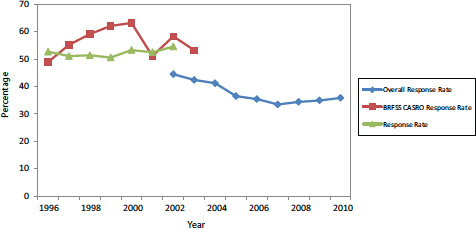
FIGURE 1-1 BRFSS median response rates.
NOTES: BRFSS = Behavioral Risk Factor Surveillance System, CASRO = Council of American Survey Research Organizations. Median rates calculated with respect to state-level results, excluding Guam, Puerto Rico, and the U.S. Virgin Islands.
SOURCE: Adapted from multiple annual issues of the Summary Data Quality Report, available by choosing individual years from http://www.cdc.gov/brfss/annual_data/annual_data.htm [May 2013].
low-response BRFSS states and therefore provided a good alternative to RDD.
BRFSS reports a response rate, a CASRO response rate, and an overall response rate (as depicted in Figure 1-1). The response rate is calculated by dividing the number of complete and partial interviews (the numerator) by an estimate of the number of eligible units in the sample (the denominator). The CASRO response rate assumes that the unresolved numbers contain the same percentage of eligible households as those records whose eligibility or ineligibility is determined. The overall response rate is more conservative in that it assumes that more unknown records are eligible and so includes a higher proportion of all numbers in the denominator (Centers for Disease Control and Prevention, 2011).
Survey of Consumer Attitudes
The SCA is a monthly telephone survey, with 500 telephone interviews of men and women living in U.S. households completed each month. The Survey Research Center at the University of Michigan uses RDD to draw the national sample for SCA. It uses a rotating panel design. The monthly
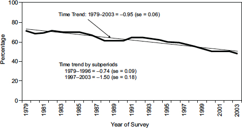
FIGURE 1-2 Changes in telephone survey response in the Survey of Consumer Attitudes.
SOURCE: Figure 1 in Curtin et al. (2005). Reprinted with permission. © Oxford University Press 2005.
samples include 300 fresh cases and 200 cases that were interviewed six months earlier.
Curtin et al. (2005) analyzed the response rates in SCA from 1979 to 2003. The response rate dropped from 76 percent in 1979 to 60 percent in 2003, an average decline of three-quarters of a percentage point per year. The rate of decline in SCA response rates is not smooth over this period, as seen in Figure 1-2, which is adapted from Figure 1 in Curtin et al. (2005).7 There was a gradual decline from 1979 to 1989, followed by a plateau from 1989 to 1996 and then a steep decline from 1996 to 2003. The authors reported opposite results for final refusals to SCA and non-contacts. Both of these factors contributed to the decline in response rates, with non-contacts driving the decline from 1979 to 1996, while the rise in refusals led to the steep decline in response rates from 1996 to 2003. The authors did not find evidence that lower unemployment or the increased use of call-screening devices in the 1990s contributed to the rise in refusals and non-contacts. They conjectured that the rapid growth in sales phone calls
______________________________________
7The response rate shown here uses every sampled phone number with the exception of those known to be ineligible in the denominator and uses partial interviews in the numerator (AAPOR response rate RR4) (Curtin et al., 2005).
and survey phone calls in the period of analysis might have contributed to the phenomenon of response rate decline in the SCA.
Census Bureau Household Surveys
The Census Bureau conducts several of the largest and most important household surveys in the federal government under the sponsorship of other federal agencies. The response rate trends that are discussed in this section pertain to the Consumer Expenditure Diary (CED) Survey, the Consumer Expenditure Quarterly (CEQ) Interview Survey, the Current Population Survey (CPS), the National Crime Victimization Survey (NCVS), the National Health Interview Survey (NHIS), and the Survey of Income and Program Participation (SIPP) during the period 1990–2008. Data for two other major surveys, the American Housing Survey–Metropolitan Sample (AHS–MS) and the American Housing Survey–National Sample (AHS–NS), are not available for the full period.
Table 1-4 shows the initial interview nonresponse rates for the years 1990 and 2009. Initial nonresponse rates are those for the first interview in multi-interview surveys. Initial nonresponse rates for all of these surveys increased, with the CED, CEQ, and CPS nonresponse rates almost doubling and the NCVS, NHIS, and SIPP nonresponse rates more than doubling. The refusal rates showed similar patterns of increase, although this category accounted for about the same or a smaller amount of overall nonresponse than it did 18 years earlier. The proportional decline in refusals has been offset by steady increases in the proportion not at home (Landman, 2009).
The nonresponse rates for the two housing surveys, which are conducted on a different time schedule than the surveys presented in Table 1-4, likewise increased. The nonresponse rates for the AHS–MS went up from 8.3 percent in 1998 to 12.7 percent in 2007, and the nonresponse rate for the AHS–NS increased from 7.8 percent to 9.6 percent over the same time span.
Bureau of Labor Statistics Household Surveys
In his presentation to the panel, John Dixon of the Bureau of Labor Statistics (BLS) compared trends in response rates for several household surveys that are sponsored by BLS; these are shown in Figure 1-3. Most of the surveys had response rates that were relatively stable over the past decade, such as the Consumer Price Index Housing Survey, which had a budget-related problem at the end of 2009 but has recovered. A notable exception is the Telephone Point of Purchase Survey (TPOPS), a commodity and services purchasing behavior survey, which has seen its response rates decline precipitously and has the worst response rates of the BLS
TABLE 1-4 Initial Nonresponse and Initial Refusal Rates in Selected Census Bureau Surveys, 1990 and 2009 (in percentage)
| Survey | Outcome Category | 1990 | 2009 |
| Consumer Expenditure Diary | Nonresponse Refusal | 16.3 8.4 | 29.7 10.8 |
| Consumer Expenditure Quarterly | Nonresponse Refusal | 12.0 9.5 | 23.6 14.3 |
| Current Population Survey | Nonresponse Refusal | 5.7 2.2 | 9.5 4.1 |
| National Crime Victimization Survey | Nonresponse Refusal | 4.3 n/a | 9.5 4.9 |
| National Health Interview Survey | Nonresponse Refusal | 4.5 2.7 | 17.8 10.8 |
| Survey of Income and Program Participation | Nonresponse Refusal | 7.3 5.3 | 19.2 12.9 |
NOTE: n/a = not available.
SOURCE: Landman (2009).
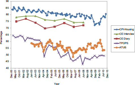
FIGURE 1-3 Response rate trends for major Bureau of Labor Statistics household surveys, December 2000–December 2010.
NOTE: ATUS = American Time Use Survey, CE Diary = Consumer Expenditure Diary, CE Interview = Consumer Expenditure Interview, CPI-Housing = Consumer Price Index-Housing, TPOPS = Telephone Point of Purchase Survey.
SOURCE: Based on figure in John Dixon presentation at panel’s workshop (Dixon, 2011).
surveys (less than 50 percent recently). TPOPS, which is conducted as an RDD survey, had a dramatic decline in its response rate in 2008, at which point its rate was less than 45 percent, but it has stabilized since then in the range of 50 percent. The American Time Use Survey (ATUS)—a telephone survey of a specific Current Population Survey household member, conducted several months after the household has completed its last CPS interview—has shown relatively low but stable rates, generally in the range of 50 to 60 percent.
Survey of Consumer Finances
The Survey of Consumer Finances (SCF) is an example of a national survey that has managed to avoid a decline in response rates over the period in which other surveys have experienced declines (Kennickell, 2007, 2010). The SCF provides data to support the analysis of the financial behavior of U.S. households and their use of financial services. It is a complex survey, collecting detailed information on a wide variety of assets and liabilities as well as data on current and past employment, pensions, income, demographic characteristics, and attitudes, with a survey design that includes collection by telephone (about 47 percent of cases are completed by phone) and personal visits. The sample is selected from two sample frames, an area-probability sample and a list sample that covers wealthy households. The overall initial sample of approximately 10,000 cases is divided approximately evenly between the two subsamples. In 2007, the area-probability sample had a response rate of 67.8 percent, while the list sample had a rate of 34.7 percent, with substantial variation in rates across the list sample strata (Kennickell, 2010). The area-probability sample rates have recovered after a period of decline in the early 1990s (see Table 1-5).
Response Rate Trends by Survey Type
The experience of this illustrative set of surveys provides evidence that nonresponse rates continue to increase in all types of cross-sectional surveys, with little to suggest that the trend has plateaued. However, the data also clearly show that the recent rates of increase in nonresponse have been substantially greater for RDD telephone surveys than for face-to-face surveys. The absolute percentage point increase for the RDD surveys is roughly three times that of the face-to-face surveys.
RESPONSE RATE TRENDS IN PANEL SURVEYS
Response rates are often seen as measures of the quality of both cross-sectional and panel surveys. Although panel studies follow a sample of
TABLE 1-5 Response Rates for the Survey of Consumer Finances, Area-Probability Sample, 1992–2010 (in percentage)
| Sample | Year | ||||||
| 1992 | 1995 | 1998 | 2001 | 2004 | 2007 | 2010 | |
| Region | |||||||
| Northeast | 65.4 | 60.1 | 62.4 | 68.7 | 61.5 | 67.5 | 65.8 |
| North Central | 68.5 | 70.9 | 67.4 | 66.9 | 69.3 | 70.3 | 72.1 |
| South | 70.3 | 67.2 | 68.3 | 70.7 | 72.5 | 68.2 | 71.3 |
| West | 66.4 | 65.3 | 63.8 | 64.9 | 68.2 | 65.0 | 63.4 |
| Area Type | |||||||
| Self-represent PSU | 61.8 | 58.9 | 62.3 | 63.2 | 65.8 | 62.2 | 65.3 |
| Other MSA | 67.4 | 66.6 | 66.6 | 69.7 | 70.4 | 74.4 | 74.4 |
| Non-MSA | 75.7 | 77.6 | 70.3 | 73.3 | 71.3 | 70.8 | 69.6 |
| All Areas | 68.0 | 66.3 | 65.9 | 68.1 | 68.7 | 67.8 | 68.7 |
NOTE: MSA = metropolitan statistical area, PSU = primary sampling unit.
SOURCE: Communication with Arthur Kennickell, U.S. Federal Reserve Board.
individuals over a long period of time and thus tend to suffer from attrition as well as initial nonresponse, the dropout rates from panel surveys, after the initial baseline entry interviews, tend to be smaller than the nonresponse rates in cross-sectional surveys. Of course, nonresponse rates in the baseline interview of panel surveys are often comparable to those in cross-sectional surveys. In this section, we discuss the response rate experience of three major panel surveys: the National Longitudinal Surveys of Youth (NLSY), the Health and Retirement Study (HRS), and the Panel Study of Income Dynamics (PSID). We use the term “retention” rates to refer to the response rates in later rounds of each survey, conditional on completing a baseline interview.
The research associated with these surveys has suggested several reasons for the generally low nonresponse rates in the later rounds of panel surveys.8 One factor leading to lower nonresponse rates may be the respondent’s familiarity with the interview format and interviewer. In a repeated survey, the respondent is aware of the kind of questions likely to be asked, the length of the interview, and the amount of effort required, because he or she has been through a similar questionnaire in the previous wave. Whatever commitment the respondent may feel to the survey may be reinforced if the same interviewer is assigned to that household
______________________________________
8Additional insight is contained in Lynn (2009), which reviewed evidence from previous research that modeled the response process within a multivariate framework and developed estimates of predictions of response from the Household, Income, and Labour Dynamics in Australia Survey.
or individual for several years. On the other hand, there is some evidence that increased prior interviewing contacts breed a familiarity with the interviewer that can depress reporting of some behaviors. Mensch and Kandel (1988) speculated that interviewer familiarity “increases salience of normative standards” and that responses are conditioned by that familiarity and also by the respondents’ expectations of a future encounter with the interviewer (p. 100).
Another possibility, drawing on sociological research on blood donation by Piliavin and Callero (1991), is that people may develop an identity as a respondent to a particular survey over time. Although they may respond for a variety of reasons initially, the more they see their participation in identity terms, the more likely they will continue in the future.
In spite of high retention rates, as dropouts accumulate, panel surveys face the risk of attrition bias in many ways. Attrition in the sample over time can reduce the sample’s representativeness and introduce bias; in addition, the loss of sample sizes over time increases the variance of the estimates. Sampling weights and refreshing the sample frame can ameliorate the effects of attrition bias, but the effectiveness of these approaches is still subject to question (Cellini et al., 2008).
There are many different response rates that can be calculated for panel surveys, and each has its separate purpose (Cheshire et al., 2011). For example, response rates can be evaluated at an aggregate (unit) level, at a wave-specific level, and as item-specific rates (Cho et al., 2004; Callegaro and DiSogra, 2008).
The National Longitudinal Surveys
The National Longitudinal Surveys are five surveys that cover different cohorts of men and women, each with the objective of collecting information on individual experiences with various life events, including employment (Bureau of Labor Statistics, 2001a, 2001b, 2002, 2006). We focus on the two most recent cohorts, which began in 1979 with a sample of people ages 14 to 22, and in 1997 with a sample of people ages 12 to 17.
The National Longitudinal Survey of Youth 1979 (NLSY79) interviews were initially conducted every year, but, starting in 1995, the survey has been conducted every other year. The interviews were conducted face to face from 1979 to 1986 and again from 1988 to 2000. In 1987, budget considerations dictated that most of the interviews be done by telephone. Telephone again became a major mode of data collection in the 2002 interview. A switch from paper-and-pencil interviewing (PAPI) to computer-assisted personal interviewing (CAPI) took place in 1993. In 2004, Web survey instruments were used for the first time in addition to the telephone
interviews. The NLSY97 interviews were initially conducted annually but are now on a biannual schedule.
Table 1-6 presents the mode of data collection and completion rates for each round of the NLSY79 survey from 1979 to 2002. In spite of changes in interview modes, completion rates (100 minus the rate shown in the last column) for NLSY79 respondents considered eligible for an interview and interviewed were in the 80–90 percent range for most of the years from 1979 to 1996, although they slipped below that level in subsequent years. The cumulative retention rate across all rounds was around 80.9 percent for living respondents. Table 1-7 documents the decreasing response and
TABLE 1-6 Type of Survey and Completion Rate for NLSY79 by Survey Year
| Year | Completed Interviews | ||||
| Personal | Telephone | Mode Not Available | Not Interviewed | Completion Rate (%) | |
| 1979 | 11,863 | 548 | 275 | — | — |
| 1980 | 11,493 | 648 | 0 | 545 | 95.7 |
| 1981 | 11,541 | 654 | 0 | 491 | 96.1 |
| 1982 | 11,066 | 1,054 | 3 | 563 | 95.6 |
| 1983 | 11,897 | 324 | 0 | 465 | 96.3 |
| 1984 | 11,422 | 646 | 1 | 617 | 95.1 |
| 1985 | 9,941 | 953 | 0 | 713 | 93.9 |
| 1986 | 9,726 | 929 | 0 | 952 | 91.8 |
| 1987 | 1,126 | 8,998 | 362 | 1,122 | 90.3 |
| 1988 | 9,494 | 920 | 51 | 1,142 | 90.2 |
| 1989 | PAPI: 8,832 | 1,469 | 3 | 1,002 | 91.4 |
| CAPI: 252 | 49 | ||||
| 1990 | PAPI: 6,972 | 1,032 | 2 | 1,171 | 89.9 |
| CAPI: 2,145 | 285 | ||||
| 1991 | 7,773 | 1,241 | 4 | 946 | 90.5 |
| 1992 | 7,848 | 1,164 | 4 | 948 | 90.5 |
| 1993 | 7,917 | 1,081 | 13 | 953 | 90.4 |
| 1994 | 7,948 | 933 | 10 | 1,073 | 89.2 |
| 1996 | 7,594 | 1,042 | 0 | 1,328 | 86.7 |
| 1998 | 6,330 | 2,069 | 0 | 1,565 | 84.3 |
| 2000 | 5,420 | 2,613 | 0 | 1,931 | 80.6 |
| 2002 | 2,317 | 5,407 | 0 | 2,240 | 77.5 |
NOTES: PAPI interviews are those conducted with paper survey instruments and pencil-entered responses; CAPI interviews are administered using a laptop computer and an electronic questionnaire that captures respondent-, interviewer-, and machine-generated data. CAPI = computer-assisted personal interviewing; NLSY79 = National Longitudinal Survey of Youth 1979; PAPI = paper-and-pencil interviewing.
SOURCE: Adapted from Table 3.3 in Bureau of Labor Statistics (2005).
TABLE 1-7 Type of Survey and Retention Rates by Round for NLSY97
| Round | Personal Interviews (%) | Telephone Interviews (%) | Total Interviewed | Retention Rate (%) |
| 2 | 94.5 | 5.5 | 8,386 | 93.3 |
| 3 | 92.0 | 8.0 | 8,208 | 91.4 |
| 4 | 91.2 | 8.7 | 8,080 | 89.9 |
| 5 | 91.5 | 8.4 | 7,882 | 87.7 |
| 6 | 83.8 | 16.2 | 7,896 | 87.9 |
| 7 | 88.0 | 12.0 | 7,754 | 86.3 |
| 8 | 87.7 | 12.3 | 7,502 | 83.5 |
| 9 | 86.5 | 13.5 | 7,338 | 81.7 |
| 10 | 88.2 | 11.8 | 7,559 | 84.1 |
| 11 | 87.4 | 12.6 | 7,418 | 82.6 |
| 12 | 85.7 | 14.3 | 7,490 | 83.4 |
| 13 | 85.9 | 14.1 | 7,559 | 84.1 |
| 14 | 88.9 | 11.0 | 7,479 | 83.2 |
NOTES: Retention rate is defined as the percentage of all base-year respondents participating in a given survey. Deceased respondents are included in the calculations. NLSY97 = National Longitudinal Survey of Youth 1997.
SOURCE: See Table 1 at http://www.nlsinfo.org/content/cohorts/nlsy97/intro-to-the-sample/interviewmethods [May 2013].
retention rates for the rounds of the NLSY97. As might be expected, retention slipped a bit from year to year.
Health and Retirement Study
The HRS is a longitudinal database of a nationally representative sample of more than 20,000 individuals over the age of 50. It is a biennial survey. The baseline data collection took place in 1992, and the sample included individuals born between 1931 and 1941 and their spouses, irrespective of the spouses’ ages. The Wave 1 response rate in 1992 was 81.6 percent. A second sample was generated to create an HRS auxiliary study known as Asset and Health Dynamics Among the Oldest Old (AHEAD). It consisted of respondents age 70 and above and their spouses. The HRS and AHEAD studies were merged in 1998. Two more cohorts—the War Baby (WB) cohort and the Children of the Depression Age (CODA) cohort—were added in the same year. The WB cohort sample consists of individuals born between 1942 and 1947, and the CODA cohort sample consists of those born between 1924 and 1930. In 2004, a new cohort was introduced, which is known as the Early Baby Boomer (EBB) cohort. The EBB sample incorporates individuals born between 1948 and 1953. The baseline response rates for AHEAD, WB, CODA, and EBB were 80.4 percent, 70 percent, 72.5 percent,
TABLE 1-8 Overall Retention Rates for Each Sample at Each Wave After the First (in percentage)
| Sample | Year(s) of Data Collection | |||||||
| 1994 | 1995/96 | 1998 | 2000 | 2002 | 2004 | 2006 | 2008 | |
| HRS | 89.4 | 86.9 | 86.7 | 85.4 | 86.6 | 86.4 | 88.6 | 88.6 |
| AHEAD | 93.0 | 91.4 | 90.5 | 90.1 | 89.4 | 90.6 | 90.7 | |
| CODA | 92.3 | 91.2 | 90.1 | 91.4 | 90.4 | |||
| WB | 90.9 | 90.6 | 87.9 | 88.1 | 87.0 | |||
| EBB | 87.7 | 86.3 | ||||||
| Total (by year) | 89.4 | 89.2 | 88.3 | 88.0 | 88.4 | 87.6 | 88.9 | 88.4 |
NOTE: AHEAD = Asset and Health Dynamics Among the Oldest Old Survey, CODA = Children of the Depression Age Sample, EBB = Early Baby Boomer Survey, HRS = Health and Retirement Study, WB = War Baby Survey.
SOURCE: National Institute on Aging (2011b).
and 68.7 percent, respectively.9Table 1-8 reports the retention rates from subsequent waves of the five samples. The baseline (first wave) response rate is based on completed interviews of all individuals deemed eligible for HRS. The wave-specific response rate is based on the number of individuals from whom an interview was sought in that wave. The declines in response rates over time that are apparent in cross-sectional surveys are not apparent here.
Most of the interviews in these five samples are conducted by telephone. Exceptions are made if the respondent has health issues or if the household does not have a telephone. Face-to-face interviews were conducted for HRS, WB, and CODA respondents in each sample’s first wave and for AHEAD respondents age 80 years and above. Mode experiments were done on AHEAD respondents in the second and third wave and on HRS respondents in the fourth wave. The mode experiment in the second wave of AHEAD compared face-to-face and telephone interviews. A similar experiment was done on HRS respondents in the birth cohort of 1918–1920. These experiments assessed the impact of interview mode on measures of cognitive functioning. The average cognitive scores of telephone-mode respondents and face-to-face mode respondents did not differ significantly in the AHEAD- and HRS-mode experiments (Ofstedal et al., 2005). In a mail-out experiment conducted on the 1998 wave of the HRS, an advance letter was sent, followed by the mail questionnaire and a $20 incentive
______________________________________
9Descriptions of HRS, AHEAD, WB, CODA, and EBB are taken from National Institute on Aging (2011b).
check; the response rate achieved was 84 percent after excluding the exit cases (National Institute on Aging, 2011b).
Panel Study of Income Dynamics
The PSID is a longitudinal household survey directed by the University of Michigan Survey Research Center. The first round of data collection took place in 1968; the sample consisted of 18,000 individuals living in 5,000 families. From 1968 to 1997, data were collected every year. In 1999 PSID started collecting data biennially. The mode of data collection changed from in-person interview to telephone interview in 1973 to reduce costs. Exceptions are made for households with no telephone or in other circumstances that do not permit a respondent to give a telephone interview. The average in-person interview was around one hour long. Despite attempts at streamlining the survey over time, the cumulative response rate dropped from 76 percent in the baseline year, 1968, to 56 percent in 1988 (Hill, 1999). Further changes were made in 1993 when PSID moved from using paper-and-pencil telephone interviews to CATI. CATI has been used for PSID ever since.
Table 1-9 shows response rates for different segments of the PSID sample for the 2003 and 2005 waves.10 A response rate of 97 percent is consistently achieved for the core segment and 88 percent for the immigrant segment. McGonagle and Schoeni (2006) documented the factors they believe are responsible for the high response rates in the PSID. These include incentive payments, payments for updating locating information during non-survey years, the use of experienced interviewers, persuasion letters sent to reluctant respondents, informing respondents about upcoming data collection waves, sending thank-you letters to responding households, and training interviewers to handle refusals. Even though response rates are exemplary in the case of the PSID relative to other panel surveys, it does suffer from high cumulative nonresponse rates due to an attrition rate of 50 percent (Cellini et al., 2008).
The reasons given by nonrespondents for not taking part in surveys have not changed much over time. A comparison of nonresponse reasons from two U.S. surveys—the 1978 National Medical Care Expenditure Survey (NMCES) and the 2008 NHIS—shows that the reasons reported
______________________________________
10The response rates are shown for two different family types—those that have remained stable (non-split-offs) and those in which family members have split off from the basic family unit to form a new family unit between waves.
TABLE 1-9 PSID Response Rates and Sample Sizes, 2003-2005
| Sample | Non-Split-Offs | Split-Offs | |||
| Response Rate (%) | Number of Interviews | Response Rate (%) | Number of Interviews | Total Number of Interviews | |
| 2003 Actual | |||||
| Core reinterview | 97 | 6,554 | 83 | 561 | 7,115 |
| Core recontact | 65 | 200 | 56 | 15 | 215 |
| Core subtotal | 95 | 6,754 | 82 | 576 | 7,330 |
| Immigrant reinterview | 94 | 459 | 61 | 36 | 495 |
| Immigrant recontact | 51 | 42 | 43 | 3 | 45 |
| Immigrant subtotal | 88 | 501 | 59 | 39 | 540 |
| Total | 95 | 7,255 | 80 | 615 | 7,870 |
| 2005 Actual | |||||
| Core reinterview | 98 | 6,756 | 89 | 516 | 7,272 |
| Core recontact | 61 | 194 | 60 | 3 | 197 |
| Core subtotal | 96 | 6,950 | 88 | 519 | 7,469 |
| Immigrant reinterview | 93 | 500 | 74 | 45 | 545 |
| Immigrant recontact | 42 | 27 | — | 0 | 27 |
| Immigrant subtotal | 88 | 527 | 74 | 45 | 572 |
| Total | 95 | 7,477 | 87 | 564 | 8,041 |
SOURCE: McGonagle and Schoeni (2006). Reprinted with permission.
TABLE 1-10 Reasons for Nonresponse from Two Face-to-Face Surveys, 1978 and 2008, in Priority Order
| NMCES Reasons for Nonresponse (1978) | NHIS Reasons for Nonresponse (2008) |
|
Not interested |
Not interested/does not want to be bothered |
|
Unspecified refusal |
Too busy |
|
No time to give |
Interview takes too much time |
|
Poor physical health/mental condition of respondent |
Breaks appointments |
|
Antipathy to surveys in general |
Survey is voluntary |
|
Wants to protect own privacy |
Privacy concerns |
|
Third-party influences respondent to refuse |
Anti-government concerns |
|
Generalized hostility to government |
Does not understand survey/asks questions about survey |
|
Other reasons |
Survey content does not apply |
|
Objects to government invasion of privacy |
Hang-up/slams door |
|
Hostile or threatens interviewer |
|
|
Other household members tell respondent not to participate |
|
|
Talk only to specific household member |
|
|
Family issues |
NOTE: NHIS = National Health Interview Survey, NMCES = National Medical Care Expenditure Survey.
SOURCE: Brick and Williams (2013, p. 39).
and their relative order were similar in the two surveys, indicating that the increase in nonresponse rates over time cannot simply be attributed to a change in subjects’ reasons for not responding (see Table 1-10).11 This suggests in turn that there is no simple way of identifying mechanisms for the increase in nonresponse rates over time by examining the reasons given for nonresponse (Brick and Williams, 2013).
When the authors examined the relationship between survey nonresponse rates and nine selected characteristics that might be expected to influence response rates by affecting accessibility or cooperation, they were able to identify four variables that were highly correlated with nonresponse rates for the four surveys they studied: the percentage of families with children under the age of six; the percentage of single-person households; the violent crime rate; and travel time to work. However, it is unclear whether these trends just happened to coincide with the increase in nonresponse rates or whether they represent causal factors in that rise.
______________________________________
11The data on the NMCES are from Meyers and Oliver (1978) based on non-interview report forms completed by field interviewers and those for the NHIS are from Bates et al. (2008) utilizing automated contact history records of verbal and non-verbal interactions recorded by interviewers during contact with households.
Groves and Couper (1998) and Harris-Kojetin and Tucker (1999) conducted similar time-series analyses. The latter study found that outside influences also played a role. The authors found evidence that changes in presidential approval, consumer sentiments regarding the economy, and the unemployment rate were reliably related to changes in refusal rates in the Current Population Survey.
THEORETICAL PERSPECTIVES ON NONRESPONSE
Survey methodologists have proposed several theories to explain why people participate in surveys. According to Goyder et al. (2006), the development of a theory of survey response has centered on several key themes: People respond to surveys when they conclude that the rewards outweigh the costs; societal factors, such as social disorganization or high crime rates, cause some respondents to refuse; different sociodemographic groups are more or less prone to take part in surveys; factors in the survey setting may influence a near-instantaneous decision; there is growing concern over intrusions on people’s time and privacy; the growth in the number of surveys has led to stronger attitudes about surveys in general, apart from topic; interviewers play a key role in gaining cooperation, especially in face-to-face surveys; the topic salience plays a role; participation is partly an emotional decision; response propensities can vary by mode of data collection; and there is a random component to these decisions. These ideas are captured to one degree or another in three main theories—social capital theory, leverage–saliency theory, and social exchange theory—which are summarized below.
Social Capital Theory
Social capital theory may help to explain the social and psychological underpinnings of the interpersonal relationships that promote trust and cooperation and thus promote the willingness to respond to surveys. According to Robert Putnam, who popularized this theory in his work (1995, 2001), social capital refers to the trust that people gain through productive interaction and that leads to cooperation. The cooperation is manifested in community networks, civic engagement, local civic identity, reciprocity, and trust in the community. Social capital can be measured in the prevalence of community organizations. The decline in association memberships in recent years is associated with less confidence in public institutions.
On an individual level, social capital is gained through education, which provides greater networking opportunities (Heyneman, 2000). Lower socioeconomic status is associated with reduced levels of trust and cooperative behavior (Letki, 2006). Other individual-level attributes affect the build-up
of social capital; in particular, length of residence, home ownership, and the presence of spouses and children strengthen social capital.
In considering the effect that social capital has on the likelihood to respond to surveys, Brick and Williams (2013) point out two aspects of the theory that should be considered: Social capital is a collective rather than an individual attribute, and the loss in social capital is partly due to generational change (p. 54). To the extent that nonresponse is generational, for example, it would suggest “exploring predictive models for reasons of nonresponse that are time-lagged and smooth data, rather than relying on the simple models that are considered here” (Brick and Williams, 2013, p. 55). Although social capital theory remains a possible explanation for increasing nonresponse, considerable research must be done to establish a link between the theory and survey nonresponse. Brick and Williams state that they would find “a rigorous investigation of the relationship between social capital and nonresponse rates to be extremely helpful” (Brick and Williams, 2013, p. 55).
Leverage–Saliency Theory
The leverage–saliency theory (LST) provides a second perspective on survey participation. Groves et al. (2004) introduced the LST of survey participation in 2000. As summarized in Maynard et al. (2010), the LST is a theory of how potential respondents make decisions to participate in a survey interview.
The LST posits that people vary in the importance and value they assign to different aspects of a survey request (Groves et al., 2000). For example, for some individuals the topic may be important, for others the reputability of the organization conducting the survey may be significant, and for still others a chance to receive a cash reward may be of consequence. According to the theory, the influence of each component of the request depends both on the weight accorded it by a sampled individual (leverage) and on its prominence in the request protocol (saliency). One application of the LST has shown that when the survey topic is a factor in the decision to participate, noncooperation will cause nonresponse error on topic-related questions (Groves et al., 2004).
The LST assumes that a potential respondent has an expected utility for participating in a survey and agrees to participate if this expected utility is net positive. “Leverage” refers to a potential respondent’s assessments (including valence and weight) of the survey’s attributes that make participation more or less appealing. For example, a cash incentive might have a positive valence and a greater weight as the size of the incentive increases; a long interview might have negative valence and a weight
that increases with the length of the interview (Dijkstra and Smit, 2002). Whether an attribute has a positive or a negative leverage varies across sample persons. A specific survey topic may have positive leverage for individuals who are more generally interested in talking about that topic and a negative leverage for those who are not (Groves et al., 2000). Likewise, different respondent groups may react differently. For example, because of different communication experiences people of different ages may be differentially sensitive to the length of a survey or to factors such as direct personal contact. There also may be strong ethnic and racial influences on a person’s assessment of the survey attributes, perhaps related to distrust of mainstream institutions. To the extent that distrust of mainstream institutions is intensifying, rising nonresponse rates may be the result.
“Saliency”—or salience—refers to the prominence of different attributes of the survey request for a sample person who is deciding whether to participate. LST calls attention to the fact that sample persons may base their decisions on only a few attributes of the survey and also to how survey organizations and interviewers provide information to sample persons. A survey might provide a financial incentive and attempt to appeal to a sense of civic duty, for example, but an interviewer might emphasize only one of these aspects, making it more salient and potentially more influential as sample persons decide whether to participate. Consequently, requests for participation in a given survey might obtain different responses from the same person, depending on which attributes are made most salient. Box 1-2 indicates how topic saliency can improve response rates.
BOX 1-2
How Topic Saliency Improves Response Rates
Judging from behavior on the first contact containing the survey introduction, we found that persons cooperated at higher rates to surveys on topics of likely interest to them. The odds of cooperating are roughly 40 percent higher for topics of likely interest than for other topics, based on the four frames utilized in the experiment. Given these results and the deductions from leverage–salience theory, we suspect we could make the 40 percent much higher by making the topic a much more salient aspect of the survey introduction. It is important to note that the overall effects on total response rates of these effects are dampened by non-contact nonresponse, as well as by physical-, mental-, and language-caused nonresponse (Groves et al., 2004, pp. 25–26).
Social Exchange Theory
Social exchange theory posits that the decision to respond to a survey is based on the assessment of the costs versus the benefits of taking part. Exchanges occur in purest form in economic transactions, and little social relationship is required for successful economic exchanges. Social exchange theory attempts to cover non-economic exchanges, where the costs and benefits include such intangibles as the maintenance of tradition, conformity to group norms, and self-esteem.
The impetus for an exchange may be as simple as “liking” the interviewer by dint of personal interaction or prepaid incentives or as complex as establishing trust. One of the founders of social exchange theory, George Homans presents exchange as overlapping with psychological heuristics. Liking may even lead to a change in opinion in accordance with the liked person’s views (Homans, 1958, p. 602).
Trust may be an important component in social exchanges. As Dillman (1978, 1991, 1999) has emphasized, in the survey setting it is important to minimize the costs to the respondents, clearly convey the nature and extent of the benefits, and establish trust so that the respondents are confident about the costs they can expect to incur and the benefits they can expect to receive. As demands on the time of respondents grow, increasing the cost of responding, and distrust of institutions multiplies, the social exchange theory would posit that nonresponse would grow unless perceived benefits of responding also increase.
IDENTIFYING COSTS ASSOCIATED WITH APPROACHES TO MINIMIZE NONRESPONSE
Costs and response trends have gone hand in hand as key driving factors in the selection of social science survey modes and in the design and conduct of surveys. As the cost of face-to-face data collection grew over the years, survey researchers moved to landline RDD data collection. As the coverage of landline RDD survey designs eroded, survey researchers shifted to dual-frame RDD designs or ABS designs. As the cost of dual-frame and ABS designs rose—and driven in part by the lack of timeliness of the latter—survey researchers were drawn to Web survey designs. It is possible that a significant portion of the downward trend in response rates is attributable to (a) survey budgets not keeping pace with rising costs even with (b) the increasing use of new frames and modes of interview to combat declining coverage. Combating declining response rates generally increases the cost of the survey, or, as stated quite succinctly in a 2004 study, “[S]urvey costs and survey errors are reflections of each other; increasing one reduces the other” (Groves, 2004, p. 49). The costs are incurred
directly in increased interviewer time and also indirectly in the increased management costs associated with approaches such as responsive design, which requires greater resources for developing and using paradata and other information systems. (Responsive design is discussed in Chapter 4.)
Peytchev (2009) examines costs in the SCA, a telephone survey where a large part of the cost is interviewer time. The number of call attempts to complete an interview in the SCA doubled between 1979 and 1996, from 3.9 to 7.9 (Curtin et al., 2005); even so, the resulting non-contact rate more than tripled during this same period. Higher proportions of non-contacts and refusals also undoubtedly require more visits and more refusal conversion attempts in face-to-face surveys.
Unfortunately, there is a dearth of evidence that relates cost to nonresponse. In an attempt to rectify this knowledge gap, in conjunction with survey sponsors, the U.S. Census Bureau has launched a major effort to identify costs associated with survey activities.12 Statistics Canada is exploring how responsive design initiatives can be employed to yield cost information that is useful for analysis and decision making.13 Both of these initiatives are in their developmental stages, but they do constitute a serious attempt on the part of these agencies to understand the costs associated with response levels, and both are aided by the collection of data during the normal survey process.
Recommendation 1-5: Research is needed to establish, empirically, the cost–error trade-offs in the use of incentives and other tools to reduce nonresponse.
It is increasingly recognized that current trends in survey costs are unsustainable. The fact that, across the Census Bureau, data collection costs have been rising as survey participation has declined led to the cost savings identification effort. Census Bureau task forces were charged with identifying the most promising opportunities to improve the cost efficiency of data collection procedures in surveys that the Census Bureau conducts for other agencies under reimbursable agreements.
Three broad themes emerged from the task forces: (1) a need for better information on costs; (2) a need for less complex survey management; and (3) a need for continuous and cooperative cost management, especially during the data collection period. In regard to the first theme, it was pointed out that, to fully understand cost trends in the field, more detailed informa-
______________________________________
12Barbara O’Hare of the U.S. Census Bureau summarized this work in her presentation to the panel on April 28, 2011.
13François Laflamme of Statistics Canada summarized this work in his presentation to the panel on April 28, 2011.
tion about how field interviewers spend their time is needed. The Census Bureau does not ask interviewers to break out their survey hours, although other survey organizations capture travel and administrative time separately from actual data collection.
One method for monitoring costs is through information about the survey process via the collection of paradata (Couper, 1998). The Census Bureau has developed the contact history instrument (CHI), which captures the characteristics of household contact attempts and outcomes; other organizations have their own call record instruments. The information collected is used by field supervisors across organizations to manage cases. Call records, such as the CHI, provide valuable information on the level of effort by case and consequently can be a good proxy for cost. There is a need to go beyond call records alone and to consolidate and systematically monitor other paradata related to costs, such as daily work hours, travel, and case dispositions. When merged with information about nonresponse rates, missing data rates, and key indicator values, costs and data quality can be evaluated simultaneously, and data collection efforts may be managed more effectively.
Despite these pioneering efforts, there is no common framework for assessing the relationship between cost and response rates and no quantitative model of the relationship. A common framework would enable the development of common metrics that would be valid across modes so that comparisons could be made and so that information on costs in an increasingly mixed-mode environment can be generated. The literature suggests that some of the cost elements and metrics that would apply to interview surveys would include information on the nature and number of contacts that people receive and on production units, such as days of interviewer project-specific training, numbers of call attempts, the length of the field period, the number of interviewers, and remuneration and incentives—all of which can be captured in paradata collecting and generating systems (see, for example, American Association for Public Opinion Research, 2010a).
Recommendation 1-6: Research is needed on the nature (mode of contact, content) of the contacts that people receive over the course of a survey based on data captured in the survey process.
In the panel’s discussion with field staff of a major ongoing survey, it became obvious that more significant costs are being incurred in the quest for high response rates.14 More expensive senior interviewers are often assigned for difficult refusal cases. Much time is spent in gaining entry to
______________________________________
14Cathy Haggerty and Nina Walker of NORC at the University of Chicago summarized their experiences in a presentation to the panel on February 17, 2011.
gated and otherwise restricted communities in the hopes of gaining an interview with a sampled unit.
Recommendation 1-7: Research is needed on the cost implications of nonresponse and on how to capture cost data in a standardized way.
These “cost” data may be based on proxy variables (such as total interviewer hours per case or other measures of effort), but at a minimum it would be useful if these or similar aggregate cost measures were routinely published. Cost information is needed if researchers are to make informed decisions about whether additional efforts to combat nonresponse are worth the cost.


