
The trends toward declining survey response rates that are documented in Chapter 1 have consequences. One key consequence is that high nonresponse rates undermine the rationale for inference in probability-based surveys, which is that the respondents constitute a random selection from the target population. Most important, nonresponse creates the potential for bias in estimates, in turn affecting survey design, data collection, estimation, and analysis. We discuss the issue of nonresponse bias in this chapter as well as the relation of nonresponse bias to nonresponse rates. We also present evidence of the impact of nonresponse on the variance of the estimates and discuss the effectiveness of conventional adjustment tools to tackle nonresponse bias. Finally, we document the need to come to a better understanding of the causes and consequences of nonresponse bias.
RESPONSE RATES MATTER, BUT . . .
In a paper initially prepared for the planning meeting for this review, Peytchev (2013) observes that drawing “unbiased inference from probability-based surveys relies on the collection of data from all sample members—in other words, a response rate of 100 percent” (p. 89). If surveys are able to register a 100 percent response rate, there is no need for adjustments in developing estimates. However, when there is nonresponse, the probability of the respondent’s inclusion is determined by both the initial probability of selection and the probability of responding.
The beauty of the response rate, most often stated as a single value for the entire survey, is that it reflects “the degree to which this goal of preserv-
ing the respondent’s inclusion probabilities is achieved” (p. 89). Peytchev contends that this fact has inarguably contributed to the widespread interpretation of the response rate as a summary measure of a survey’s representativeness. However, response rates can be misleading as measures of survey representativeness. The fact that response rates have fallen (as documented in Chapter 1) means only that the potential for nonresponse bias has increased, not necessarily that nonresponse bias has become more of a problem. That is because nonresponse bias is a function of both the nonresponse rate and the difference between respondents and nonrespondents on the statistic of interest, so high nonresponse rates could yield low nonresponse errors if the difference between respondents and nonrespondents is quite small or, in survey methodology terms, if nonresponse in the survey is ignorable and the data can be used to make valid inferences about the target population.
Moreover, it would be a relatively simple matter to overcome the problem of bias in the estimates brought about by nonresponse if there were a linear relationship between response rates and nonresponse bias across surveys. If it were so, one could theoretically reduce nonresponse bias by taking actions to increase response rates, and more effort, cost, training, and management control of the survey operation would solve the problem. This is not the case, however, as shown by Curtin et al. (2000), Groves et al. (2006), and Groves and Peytcheva (2008). The 2008 Groves and Peytcheva compilation of the results of 59 specialized studies found very little correlation between nonresponse rate and their measures of bias. Likewise, there is no proof that efforts to enhance response rates within the context of a survey will automatically reduce nonresponse bias on survey estimates (Curtin et al., 2000; Keeter et al., 2000; Merkle and Edelman, 2002; Groves, 2006).
Recommendation 2-1: Research is needed on the relationship between nonresponse rates and nonresponse bias and on the variables that determine when such a relationship is likely.
It is possible that extraordinary efforts to secure responses from a reluctant population may even increase bias on some survey estimates (Merkle et al., 1998). A 2010 study by Fricker and Tourangeau suggested that efforts to increase response can lead to quality degradation. The authors examined nonresponse and data quality in two national household surveys: the Current Population Survey (CPS) and the American Time Use Survey (ATUS). Response propensity models were developed for each survey. Data quality was measured through such indirect indicators of response error as item nonresponse rates, rounded value reports, and interview–response inconsistencies. When there was evidence of covariation between
response propensity and the data quality indicators, potential common causal factors were examined. The researchers found that, in general, data quality, at least as they measured it, decreased for some variables as the probability of nonresponse increased. The study concluded that efforts to reduce nonresponse can lead to poorer quality data (Fricker and Tourangeau, 2010). Other work in this field is under way and may shed additional light on this important issue.
Recommendation 2-2: Research is needed on the impact of nonresponse reduction on other error sources, such as measurement error.
Recommendation 2-3: The research agenda should seek to quantify the role that nonresponse error plays as a component of total survey error.
Although the exact relationship between nonresponse and bias is not yet clear, it is still important to understand the effects of nonresponse bias because bias jeopardizes the accuracy of estimates derived from surveys and thus the ability of researchers to draw inferences about a general population from the sample. The interactions are complex because nonresponse exists at the item level as well as at the interview level, and item nonresponse contributes to bias at the item-statistic level so that bias is a function of both unit and item nonresponse.
Recommendation 2-4: Research is needed to test both unit and item nonresponse bias and to develop models of the relationship between rates and bias.
Examples cited in Peytchev (2009) and other sources (e.g., Groves, 2006; Groves and Peytcheva, 2008) tend to show that the effect of nonresponse bias on means and proportions can be substantial:
• Nonrespondents to the component of the National Health and Nutrition Examination Survey III that measured glucose intolerance and diabetes through eye photography were 59 percent more likely to report being in poor or fair health than respondents to the main survey (Khare et al., 1994).
• The Belgian National Health Interview Survey with a response rate of 61.4 percent obtained a 19 percent lower estimate for reporting poor health than did the Belgian census, which had a response rate of 96.5 percent (Lorant et al., 2007).
• A comparison of the results of a five-day survey employing the Pew Research Center’s usual methodology (with a 25 percent response rate) with results from a more rigorous survey conducted over a much longer field period and achieving a higher response rate of 50 percent found that, in 77 out of 84 comparisons, the two surveys yielded results that were statistically indistinguishable. Among the seven items that manifested significant differences between the two surveys, the differences in proportions of people giving a particular answer ranged from 4 percentage points to 8 percentage points (Keeter et al., 2006).
• An analysis of data from the ATUS—the sample for which is drawn from the CPS respondents—together with data from the CPS Volunteering Supplement was undertaken to demonstrate the effects of survey nonresponse on estimates of volunteering activity and its correlates (Abraham et al., 2009). The authors found that estimates of volunteering in the United States varied greatly from survey to survey and did not show the decline over time common to other measures of social capital. They ascribed this anomaly to social processes that determine survey participation, finding that people who do volunteer work respond to surveys at higher rates than those who do not do volunteer work. As a result, surveys with lower response rates will usually have higher proportions of volunteers. The result of the decline in response rates over time likely has been an increasing overrepresentation of volunteers. Furthermore, the difference shows up within demographic and other subgroups, so conventional statistical adjustments for nonresponse cannot correct the resulting bias.
• In a study of nonresponse bias for the 2005 National Household Education Survey (NHES), Roth et al. (2006) found evidence of a potential bias in the survey on adult education, in which females were more likely to respond than males were. The problem was resolved by a weighting class adjustment that used sex in forming the weighting classes.
• In another study of nonresponse bias in the 2007 NHES (Van de Kerckhove et al., 2009), results indicated undercoverage-related biases for some of the estimates from the school readiness survey. However, nonresponse bias was not a significant problem in the NHES data after weighting.
Recommendation 2-5: Research is needed on the theoretical limits of what nonresponse adjustments can achieve, given low correlations with survey variables, measurement errors, missing data, and other problems with the covariates.
Nonresponse can also affect the variance of any statistic, reducing confidence in univariate statistics, and it can also bias estimates of bivariate and multivariate associations, which could bias results from substantive
analyses. These effects can be significant. The factors that could affect the variances are the underlying differences between respondents and nonrespondents in levels of variability, differences in respondent and nonrespondents means, uncertainty introduced by adjustments, and the variability in the number of interviewed respondents. All things considered, it is not clear whether nonresponse will generally cause variability to be understated or overstated.
The effect of nonresponse bias on associations is not clear, and, in Peytchev’s (2009) view, it has been understudied. Peytchev observed that, to the extent that it has been studied, nonresponse bias in associations appears to be different from bias in means and proportions in that, even when there is substantial bias in means, there may be no nonresponse bias in bivariate associations.
There is a strong relationship between survey costs and nonresponse. On one hand, survey managers have intensified data collection activities in order to improve response rates. On the other hand, the trend toward higher survey costs has led to shortcuts, shortened collection periods, and cheaper modes that have had effects on survey response rates. The costs have been monetary and have also appeared in terms of data utility. Addressing nonresponse through a two-phase sample, for example, can increase the design effect in weighted estimates, producing a lower effective sample size than a comparable single-phase design. The problem of nonresponse can lead to survey designs of increasing complexity because accounting for nonresponse is becoming essential for the measurement and reduction of nonresponse bias. This is evident in the elaborate and dynamic responsive designs (Groves and Heeringa, 2006) that are now being implemented, in which design decisions are informed by deliberate variations in early recruitment protocols and careful monitoring of cost and error indicators during data collection. Some designs attempting to reduce nonresponse and keep costs under control are also incorporating multiple modes, as sample members exhibit different response propensities for different modes, and modes vary in cost structure. Some modes require separate sampling frames. Since combinations of sampling frames and modes yield higher response rates, the use of multiple sampling frames is also increasingly being considered. These designs are further discussed in Chapter 4.
Another consequence of growing nonresponse and the cost associated with improving response rates is an increase in the reliance of probability-based survey estimates on models that use auxiliary data. Some external data already exist on individuals in the population, but these data may be underutilized in surveys. External data can be found in administrative databases, in databases compiled by commercial vendors, and in the public domain. Some pioneering efforts to increase the use of auxiliary data for
reducing the effect of nonresponse are discussed in Chapter 4. Likewise, the need to better understand the sources of nonresponse has led to an explosion in efforts to collect and analyze paradata—that is, data that document the survey process (call records, timing of call attempts, interviewer–respondent interactions, interviewer performance measures, and the like). Such measures can be collected by interviewers or directly by survey systems. Current challenges associated with paradata are the identification of what data elements to collect and how to organize such data structures in order to aid data collection and the creation of post-survey adjustments.
One use of paradata has been to gain a better understanding of the characteristics of “converted” respondents (i.e., those who were persuaded to take part after refusing initially), other respondents who were difficult to include in the survey, partial completers, and those who break off their survey responses versus those who complete interviews. The purpose is to test the assumption that reluctant sample members and those who do not complete the interview are more similar to nonrespondents than to respondents (Lin and Schaeffer, 1995; Bose, 2001). The advances in understanding and improving response rates through use of paradata are further discussed in Chapter 4.
NONRESPONSE BIAS IN PANEL SURVEYS
The problem of nonresponse bias in longitudinal panel surveys can be framed differently from the problem of nonresponse bias in non-repeated surveys. Longitudinal surveys suffer from attrition as well as initial nonresponse. Attrition is a form of nonresponse—that is, losing sample members from one collection wave to subsequent waves can produce nonresponse biases, just as in cross-sectional surveys.
Although still a substantial challenge, the characteristics of panel surveys are more amenable to understanding (and perhaps adjusting) for nonresponse. While bias in the first wave of data collection may persist in future rounds of data collection (Bose, 2001) and be exacerbated by attrition in later rounds, after the first wave of data collection, much is known about the characteristics, survey experiences, and response patterns of those who fail to respond to subsequent rounds. In a longitudinal study, once data have been collected in the base year from respondents, nonrespondents in subsequent rounds can be compared to respondents in those rounds using the base-year data as well as the frame data. Using this information, it is possible to understand, and adjust for, nonresponse bias. Still, understanding the amount and impact of nonresponse bias from survey attrition and from baseline nonresponse remains a challenge.
As nonresponse has grown, so has interest in developing methods to estimate nonresponse bias and to adjust for it (Billiet et al., 2007; Stoop et al., 2010). For the surveys sponsored by the U.S. government, this interest has been driven, in part, by Office of Management and Budget requirements that “sponsoring agencies conduct nonresponse bias analyses when unit or item response rates or other factors suggest the potential for bias to occur” (Office of Management and Budget, 2006, p. 8, italics added). The thresholds that trigger a nonresponse bias analysis are an expected unit response rate of less than 80 percent or an item response rate of less than 70 percent.
The purpose of the analysis is to ascertain whether or not the data are missing completely at random. There are several approaches for determining this:
• Multivariate modeling of response using respondent and nonrespondent frame variables to determine if nonresponse bias exists.
• Weighting the final sample using population figures for background variables (i.e., using post-stratification) and comparing the weighted results with unweighted results to identify those variables that might be particularly prone to bias.
• Comparison of the characteristics of the respondents to known characteristics of the population in order to provide an indication of possible bias. However, a Federal Committee on Statistical Methodology study concluded that these comparisons should be used with caution because some of the differences between the respondent and population data may be due to measurement differences (including differences in coverage and content), true changes over time, or errors in the external sources (Office of Management and Budget, 2001). Estimates from large multipurpose surveys such as the American Community Survey and the Current Population Survey are often used in these comparisons, as are administrative record data sources.
• Using interviewer observation data, such as ratings of dwellings and neighborhood information as observed and recorded by the interviewers. These data are used as a proxy for individual household data in ascertaining whether respondents differ in important respects from nonrespondents and whether reluctant respondents differ from more cooperative respondents.
• Collecting information from nonrespondents in a follow-up survey to measure how they differ from respondents. There are a wide variety of techniques used in follow-up surveys, but most collect some key variables either from all or a randomly selected sample of nonrespondents. As might be expected, it is critical to have high response rates in follow-up surveys.
Follow-up surveys tend to be expensive because of the very intensive nonresponse conversion techniques that are employed to minimize nonresponse in the follow-up sample.
Recommendation 2-6: Research is needed to improve the modeling of response as well as to improve methods to determine whether data are missing at random.
NEW METRICS FOR UNDERSTANDING NONRESPONSE BIAS
The response rate is still useful for many reasons. It is reported at the survey level, and it documents differences between surveys. It has become ingrained, and survey sponsors and academic journals have established response rate requirements. It is also a useful tool for managing fieldwork. For these reasons, it is likely that response rates will remain an important indicator of data quality.
However, the response rate has serious shortcomings. It is not directly linked to bias. It is also not variable specific. Most important, its use in field operations may distort data collection practices—for example, by suggesting that interviewers should attempt to interview the remaining cases with the highest response propensity, which is not necessarily a strategy that will reduce bias.
Because the nonresponse rate can be such a poor predictor of bias, researchers have turned to developing new metrics for depicting the risk of nonresponse bias. This is not without its own dangers, and moving the focus from the response rate to more abstract measures may have unintended consequences. For example, interviewers hearing that “response rates don’t matter” might mistakenly infer that their efforts to obtain relatively difficult cases did not matter. Moreover, because nonresponse bias is specific to a particular estimate (or model) and not to a survey in general, there could be confusion about the quality of a survey to support estimates other than those for which nonresponse bias has been studied.
Those interested in developing alternative indicators of bias have generally turned to two typologies: those at the survey level and those that pertain to estimate levels. Wagner (2008, 2011) proposed a typology that separates response rate from other survey-level indicators, identifies the data involved, and differentiates indicators based on implicit and explicit model assumptions. These indicators can be further differentiated as those using a response indicator (i.e., response rate); those using a response indicator and frames and paradata; and those using a response indicator, frames and paradata, and a survey variable or variables.
Researchers have increasingly recognized that indicators that also use paradata have some advantages. Examples of attempts to construct this
class of indicators include a comparison of respondents and nonrespondents on auxiliary variables, variance functions of nonresponse or post-stratification weights, and goodness-of-fit statistics of propensity models (Schouten et al., 2009). They utilize more data and are reported at the survey level. But, like response rates, they are mainly useful only in the context of a specific survey, whereas nonresponse bias is a statistics-level problem. As a result, they are not commonly used.
Representativity indicators (R-indicators) are an example of a new metric for assessing the effects of nonresponse.1 R-indicators attempt to measure the variability of response propensities (van der Grijn et al., 2006; Cobben and Schouten, 2007). They do this by measuring “the similarity between the response to a survey and the sample or the population under investigation” (van der Grijn et al., 2006, p. 1). A survey that exhibits less variability in response propensities is likely to exhibit a better match between the characteristics of the respondents and the population they are meant to represent for the variables that the model uses to estimate the propensities.
R-indicators can be monitored during data collection to permit survey managers to direct effort to cases with lower response propensities and, in so doing, to reduce the variability among subgroup response rates. The indicator can be monitored during survey collection because the response propensities can be calculated with complete information available on the frame. In order for the R-indices to be completely comparable across surveys, they need to be estimated with the same variables. Wagner (2008) suggests that this would be facilitated if all surveys had a common set of frame data. However, there is no proof that such indices would apply across all types of surveys, or even across all relevant estimates within a given survey. More research that uses these indicators in survey settings is needed.
An example of the use of the R-index was provided by John Dixon of the Bureau of Labor Statistics in his presentation to the panel (Dixon, 2011). As shown in Figure 2-1, he charted the R-index for the Current Population Survey (top line) with the response rate for the survey (bottom line). He noted that, at 95 percent confidence intervals, the R-index is somewhat flatter than the response rate, which suggests that, for this survey, response propensities indicate a good match between the characteristics of the respondents and the population they are meant to represent.
Estimate-level indicators are indicators that use a response indicator, frame and paradata, and survey variables. They require an explicit model for each variable, and the model is usually estimated from the observed data and relies on the assumption that the missing data are missing at random (MAR). Wagner reported that there is very little research into non-MAR
______________________________________
1Additional content on R-indicators is provided by Wagner (2011).
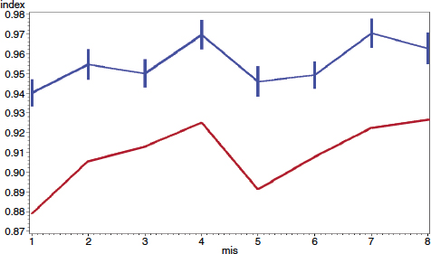
FIGURE 2-1 Plot of R-index (top line) and response rate (bottom line) for Current Population Survey cohorts by months in sample.
NOTE: Top line includes 95 percent confidence interval error bars around month-in-sample (mis) values for the R-index.
SOURCE: John Dixon presentation to the panel (Dixon, 2011).
assumptions, citing the work of Andridge and Little (2009) as an exception. This method also calls for the filling in of missing data. The results are valid within the context of the survey, but they are not necessarily comparable across surveys and, as a result, this method is not commonly used. Examples of these indicators are the correlations between post-survey weights and survey variables, variation of means across the deciles of survey weights, comparisons of early and late responders, and the fraction of missing information (FMI). The FMI is computed within a multiple imputation framework (Rubin, 1977) in which the model relates the complete frame data and paradata to the incomplete survey data. The FMI is the ratio of the imputation variance to total variance.
Balance indicators (B-indicators) were introduced by Särndal (2011) in a presentation at the annual Morris Hansen Lecture. They are an alternative indicator of bias—a measure of the lack of balance between the set of respondents and the population. The degree of balance is defined as the degree of fit between the respondent and population characteristics on a (presumably) rich set of frame variables. Särndal introduced a concept of a balanced response set, stating, “If means for measurable auxiliary
variables are the same for respondents as for all those sampled, we call the response set perfectly balanced” (p. 4). The B-indicator can be used to measure how effective techniques for improving the balance of the sample, such as responsive design (see Chapter 4), have been.
In addition to the R-indicators and B-indicators, other indicators could be imagined, such as a measure based on the variance of the weights. Such indicators are promising, but, as Wagner reminded the committee, a research agenda on alternative indicators of bias should include research on the behavior of different measures in different settings, the bounds on nonresponse bias under different assumptions (especially non-MAR), how different indicators influence data collection strategies, and how to design or build better frames and paradata.
Recommendation 2-7: Research and development is needed on new indicators for the impact of nonresponse, including application of the alternative indicators to real surveys in order to determine how well the indicators work.
NEED FOR A THEORY OF NONRESPONSE BIAS
This chapter describes a large and growing body of research into the characteristics of nonresponse bias and its relationship (or lack of relationship) to response rates. While encouraging, the work has gone forward in piecemeal fashion and has not been conducted under an umbrella of a comprehensive statistical theory of nonresponse bias.
In his presentation to the panel, panel member Michael Brick suggested that a more comprehensive statistical theory would enhance the understanding of such bias and aid in the development of adjustment techniques to deal with bias under different circumstances (Brick, 2011). A unifying theory would help ensure that comparisons of nonresponse bias in different situations would lead to the development of standard measures and approaches to the problem. In the next chapter, the need for a comprehensive theory will again be discussed, this time in the context of refining overall adjustments for nonresponse.


