
The committee was asked to consider various issues associated with models, geospatial data, mixtures, and uncertainty. Although the language of the task statement was focused on effects analysis, determining which effects might be relevant requires estimating exposure. In this chapter, the committee first discusses fate and transport models used in exposure analyses by the agencies and then provides suggestions for a stepwise approach to estimating environmental concentrations of pesticides in the context of complying with the Endangered Species Act (ESA). Next, the committee addresses what constitutes authoritative geospatial data—critical information used to conduct exposure modeling and define species’ habitats—and provides some examples. Finally, the committee discusses some important uncertainties associated with exposure analysis and the need to propagate uncertainty through the analysis.
If pesticides are to be used without jeopardizing the survival of listed species and their habitats, the estimated environmental concentrations (EECs) to which the organisms and their habitats will be exposed need to be determined. Chemical fate and transport models are the chief tools used to accomplish that task. Broadly, such a model requires a user to choose a series of environmental control volumes—that is, environmental compartments containing multiple media, such as air, water, and soil—that are assumed to have a single, homogeneous pesticide concentration at each time step of the model. The transport and transformation processes that might affect a pesticide’s presence in each control volume are combined and assembled into a mass-balance model that allows estimation of the EECs. Typically, the fate processes, such as sorption and biodegradation, are mathematically expressed in such a way that they can be adjusted by using chemical-specific and environment-specific information. However, knowledge or information can be insufficient, so the model parameter values for some chemical or physical processes are often oversimplified. For example, the distribution of a pesticide between the solids and water in a single compartment might be quantified by using a linear adsorption isotherm, although the data might suggest that the pesticide sorption mechanism exhibits nonlinear behavior.
Because the pathways by which pesticides move from their points of application to habitats of listed species might involve a complex sequence of transfers and diverse degradation processes, it is common to use a linked series of models to estimate exposure. Fate and transport modeling practices used by the US Environmental Protection Agency (EPA), Fish and Wildlife Service (FWS), and National Marine Fisheries Service (NMFS) are discussed below. The committee also elaborates on its suggestions for analyses that comply with Steps 1-3 in the ESA process when estimating exposure (see Table 2-1).
Approaches and Models Used by the Agencies
In Step 1 of the ESA process, EPA uses a program called DANGER to determine which listed species or their habitats coincide geographically and temporally with areas of pesticide use (EPA 2012a).1 DANGER is an electronic database of county-level information on occurrence of listed species and acreage of agricultural crops. If there is geographic and temporal overlap, EPA assumes a “may affect” for pesticide use and addresses the listed species during its pesticide risk assessment (Step 2), in which pesticide concentrations are estimated in the environmental media to which the species might be exposed, as discussed below.
In Step 2 of the ESA process, EPA first uses a generic screening model to determine whether the pesticide is likely to move off the crop and into a body of water in concentrations high enough to trigger a concern for any aquatic species. For that initial screen, EPA uses GENEEC2 (Generic Estimated Environmental Concentration) (EPA 2001), a model that estimates pesticide concentrations in a standard small farm pond (a 2-m deep pond that has a surface area of 1 hectare in a watershed area of 10 hectares), uses generic inputs, and simulates a single event. Few fate processes are considered in the model. EPA typically assumes the maximum pesticide application rate as allowed by the label, and the model estimates pesticide concentration in the pond on the basis of spray drift and runoff from a 6-in. rain event that lasts 24 h.
As a screening model, GENEEC is sometimes characterized as providing worst-case estimates of exposure. The term worst-case, however, is misleading and should be avoided. The documentation for the model does not use the term worst-case but states that GENEEC “may provide a good predictor of upper level pesticide concentrations in small but ecologically important upland streams” (EPA 2001). That conclusion is attributed to Effland et al. (1999), but they discuss general monitoring data in streams rather than specific field studies that might be used to evaluate the accuracy of GENEEC with respect to specified applications.
______________________
1The committee understands that EPA now commonly refers to the DANGER database as LOCATES (A. Pease, EPA, personal commun., May 13, 2013).
If the initial screening assessment triggers a concern for any aquatic species, EPA uses more sophisticated models, such as the Plant Root Zone Model (PRZM3; Suarez 2005) and the Exposure Analysis Modeling System (EXAMS; Burns 2004), to estimate pesticide concentrations in surface waters (EPA 2012b, c). Again, the standard farm field (10 hectares) and pond (1 hectare) scenario is typically modeled, but the models incorporate more fate processes and simulate effects of daily weather variability over multiple years. For example, the initial spatial fallout of a pesticide sprayed via aircraft into air over a field is estimated with a model, such as AgDRIFT ® (Teske et al. 2002; SDTF 2010). The AgDRIFT-derived estimates then serve as inputs into PRZM3, which assesses pesticide fate in the soil environment, including evaporation to the atmosphere, infiltration into the subsurface, and off-site transport via overland runoff. Finally, to the extent that the combination of AgDRIFT and PRZM3 (which includes the Vadose Zone Flow and Transport model subroutine) yields estimates of pesticide delivery to nearby surface waters, EXAMS is used to estimate the temporally changing chemical concentrations in those waters and their underlying sediments. The resulting estimated concentrations in soil, water, and sediment yield estimates of the pesticide exposure of receptors of interest, including listed species.
For terrestrial species, EPA models pesticide exposure with the Terrestrial Residue Exposure (T-REX) model, the TerrPLant model, the Screening Imbibition Program (SIP) model, and the Screening Tool for Inhalation Risk (STIR) model (EPA 2012d). Exposure of terrestrial species is assumed to be through the diet, which is simulated by the exposure routine in T-REX. The model calculates pesticide residue concentrations on various food items (for example, short grass and broad-leafed plants) on the basis of work by Hoerger and Kenaga (1972) as modified by Fletcher et al. (1994) at a daily interval for 1 year. Other parts of the T-REX model translate exposure concentrations into daily doses for hypothetical small, medium, and large birds and mammals on the basis of food intakerate equations from EPA’s Wildlife Exposure Factors Handbook (EPA 1993). More recently, EPA has begun to estimate wildlife exposure through drinking water with the SIP model and inhalation with the STIR model. Those models are intended for use during problem formulation to determine whether the alternative exposure routes should be considered in the aggregate with food ingestion. SIP assumes that water concentrations are at the limit of solubility, and drinking-water ingestion rates are from Nagy and Peterson (1988). STIR calculates vapor-phase exposure from chemical-specific properties, such as molecular weight and vapor pressure, and includes estimates of spray-droplet exposure. Maximum inhalation rates are from EPA (1993), and the model assumes that a small-bodied bird or mammal is exposed to saturated air. For terrestrial plants, exposure for screening-level assessments of single pesticide applications is estimated by TerrPLant by assuming runoff delivery from a treated dry acre of land to a neighboring untreated acre, runoff from 10 treated acres to a 1-acre neighboring wetland, or specified percentages of spray drift after ground and aerial applications.
In Step 3, the Services also calculate environmental exposures with the same models that EPA uses in Step 2. For example, GENEEC2 was used in some of the biological opinions (BiOps) reviewed by the committee (NMFS 2008, pp. 235ff; 2009, pp. 284ff; 2010, pp. 294ff) as was AgDRIFT (NMFS 2008, p. 228). The committee did not examine any BiOps on terrestrial organisms, so it cannot comment on the terrestrial-exposure models used by the Services. However, the model input parameters used by NMFS to estimate aquatic exposure concentrations differ from those used by EPA, and the model is modified to estimate input into waters other than the standard farm pond. Those differences account for regional and habitat differences that are specific to the listed species and are discussed further in the next section.
A Stepwise Approach to Fate and Transport Modeling
Mass-balance models for chemical exposure analyses have several strengths. First, principles of mass-balance modeling and computer-simulation programs are well established. Second, many exposure models—such as Ag-DRIFT, PRZM, and EXAMS—are well documented. Third, the models can be made case-specific by time-varying data, such as meteorological conditions. Fourth, the output of one model can be used as input into the next one; for example, EXPRESS is a linked EXAMS-PRZM Exposure Simulation Shell (Burns 2006).
However, the model limitations need to be recognized, and models need to be used in the appropriate contexts. For example, GENEEC2 was developed by EPA simply as an easy-to-use screening tool to provide a consistent approach in the conduct of screening-level assessments, such as in Step 1 (or early in Step 2) of the ESA process (see Table 2-1). Although the Services have used GENEEC2 in BiOps, the committee concludes that a screening-level model has no place in Step 3 of the ESA process, in which the Services need to conduct a direct assessment of risk to a listed species. The GENEEC2 model has no provision for site-specific or region-specific inputs, such as soil characteristics, slopes, and meteorological data. Furthermore, with the development of simple-to-use implementations of PRZM/EXAMS for the farm pond and index reservoir (PRZM/EXAMS Express, Burns 2006), there seems to be little need for or practical value of GENEEC2. For Steps 2 and 3, EPA and the Services should be using region-specific or site-specific applications of PRZM/EXAMS or possibly more sophisticated watershed models.
As noted in Chapter 2 (see Table 2-1), the committee suggests a common approach that involves more refined and sophisticated modeling and analysis as one progresses from Step 1 to Step 3 in the ESA process. Given the current practices in exposure analysis and the need to estimate pesticide exposures and the associated spatial-temporal variations experienced by listed species and their habitats, the committee envisions the following stepwise approach to exposure modeling.
• Step 1 (EPA). Initial exposure modeling would answer the question, Do the areas where the pesticide will be used overlap spatially with the habitats of any listed species? The Services, which have extensive knowledge of the natural history of listed species, could help EPA to identify overlaps of areas where a pesticide might be used and the habitats of listed species. EPA’s DANGER program would be useful in this step.
• Step 2 (EPA). If area overlaps are identified in Step 1, EPA would confer with the Services to identify relevant environmental compartments (for example, pond vs stream), associated characteristics (for example, sandy vs silty soils), and critical times or seasons in which environmental exposure concentrations need to be estimated. With that knowledge, suitable model parameter values could be chosen and used. The goal of EPA’s initial exposure modeling would be to identify the most important environmental compartments for exposure modeling (water, soil, air, or biota). Models—such as GENEEC2, SIP, and SPIR—would be useful in this step. If the models indicate that substantial amounts of pesticides move off the application site and into the surrounding ecosystems, more sophisticated fate and transport processes could be incorporated. At that point, the pesticide-fate model could be simplified to remove processes that are unimportant in the specific regions of the listed species and set up to estimate time-varying and space-varying pesticide concentrations in typical habitats (for example, 10-cm-deep shallow regions along streams vs 2-m-deep farm ponds) with associated uncertainties. The committee emphasizes that inputs should include statistical distributions of each parameter to enable probabilistic modeling of exposure scenarios. During Step 2, EPA could direct the terrestrial exposure modeling at specific size classes of taxonomic groups that represent the listed species of concern. On the basis of the modeling results, EPA could then make a decision about the need for formal consultation with the Services.
• Step 3 (Services). During a formal consultation, the Services would further refine the exposure models to develop quantitative estimates of pesticide concentrations and their associated distributions for the particular listed species and their habitats. To that end, the models would use site-specific input values—for example, actual pesticide application rates, locally relevant geospatial data to characterize such quantities as wind speed and organic contents of soils, and time-sensitive life stages of listed species. The exposure analysis would be completed with propagated errors on exposure estimates.
Some issues associated with the exposure models or modeling practices need to be emphasized. First, pesticide-fate models are not always well tested with field data for specific pesticide applications at sites whose properties are knowable. Bird et al. (2002) tested AgDRIFT, and Loague and Green (1991) tested PRZM. However, a comprehensive treatment of the use of EXAMS with pesticides is largely lacking. Burns (2001) did list six studies involving field observations of diverse compounds that could be compared with EXAM model-
ing expectations, but none of the data involved pesticides applied in agricultural settings except the use of sulfonyl herbicides in rice fields. To evaluate and improve the accuracy of the exposure estimates, one could pursue a measurement campaign specifically coordinated with several pesticide field applications in a few case-specific examples during Step 3 exposure modeling. The exposure estimates should be compared with pesticide measurements in various environmental media, and modeling should be revised if measurements deviate substantially from selected statistical bounds, such as two standard deviations, of modeled estimates of environmental concentrations.
The committee notes that in evaluating models, general monitoring data and field studies need to be distinguished. General monitoring studies (see, for example, Gilliom et al. 2007) provide information on pesticide concentration in surface water or ground water on the basis of monitoring of specific locations at specific times. The monitoring reports, however, are not associated with specific applications of pesticides under well-described conditions, such as application rate, field characteristics, water characteristics, and meteorological conditions. General monitoring data cannot be used to estimate pesticide concentrations after a pesticide application or to evaluate the performance of fate and transport models.
Second, the model predictions can be only as accurate as the parameter estimates. If the relevant parameter values and their variances are poorly known, the model predictions will be uncertain and difficult to use in decision-making. That shows the need to identify the key processes and to ensure that the parameter values associated with the key processes are well known. The committee notes that although this is not typically done, exposure models can be used to identify the most important fate processes for a given pesticide application. For example, Sato and Schnoor (1991) used EXAMS to study the fate of dieldrin delivered by runoff to an Iowa reservoir. The pesticide’s fate was dominated by flushing and bed-water exchange, so dieldrin exposures were sensitive to the depth of the mixed bed, and getting that parameter right was necessary to achieve accurate modeling. Similarly, Seiber et al. (1986) found that volatilization of 2-methyl-4-chlorophenoxyacetic acid from rice fields did not result chiefly from water-to-air exchanges but rather from transfers of salts dried on foliage to the air. Such key chemical fate processes, once identified, are almost never pursued in sufficient detail to allow substantial improvement in exposure modeling. Although studies by pesticide registrants might yield useful site-specific information, the empirical observations do not typically yield generalizable understandings of fate processes that can be readily used in new situations without introduction of further uncertainty.
Finally, the committee notes that the pesticide fate and transport models do not provide information on the watershed scale; they are intended only to predict pesticide concentrations in bodies of water at the edge of a field on which a pesticide was applied. Different hydrodynamic models are required to predict how pesticide loadings immediately below a field are propagated through a watershed or how inputs from multiple fields (or multiple applica-
tions) aggregate throughout a watershed. Watershed-scale models, such as the Soil and Water Assessment Tool (SWAT), have been developed to predict the effects of agronomic practices on water and sediment. SWAT operates on a daily time step and can perform simulations over a long time (30 years) by using physical landscape characteristics (including soil types and topography), data on land cover and land use, weather data, and physical-chemical properties of compounds to simulate processes that dictate routing of water and sediment. The primary routes for chemicals to enter water from a site of application in SWAT are surface runoff and infiltration of applied chemicals into groundwater that can reach surface waters through lateral flow and recharge. Thus, SWAT has an interface with PRZM/EXAMS or the Groundwater Loading Effects of Agricultural Management Systems (GLEAMS) (Leonard et al. 1989; Knisel and Davis 2000) model and can be used to predict chemical concentrations at particular points in a watershed over variable intervals.
GEOSPATIAL DATA FOR HABITAT DELINEATION AND EXPOSURE MODELING
Geospatial data are critical for exposure modeling and for describing species’ habitats. The committee was asked to consider what constitutes authoritative geospatial data. The following sections discuss the delineation of habitat, describe the criteria for authoritative geospatial data, and provide several examples of various types of authoritative geospatial data.
Characterization and Delineation of Habitat
Habitat refers to the abiotic and biotic environmental attributes in an area that allow an organism to survive and reproduce (Hall et al. 1997). Habitat configuration, area, and quality—which vary over space and time—affect probabilities of persistence of populations and species. Because habitat by definition supports survival and reproduction, the term suitable habitat is redundant, and the term unsuitable habitat is contradictory. Habitat is species-specific, although a specific abiotic or biotic attribute might be a habitat component for multiple species; habitat is not synonymous with land cover, vegetation, or vegetation structure (Hall et al. 1997). Detailed explanations and discussions of the concept of habitat are included in Fretwell (1972), Morrison and Hall (2002), and Mitchell (2005). Characterization and delineation of species’ habitats is necessary to estimate where and when a given pesticide and a given species might co-occur, to make spatially and temporally explicit calculations of pesticide exposure, and to specify the spatial structure of population models used in effects analyses.
The first step in delineating habitat is to compile data on species occurrence and, ideally, data on species’ demography and environmental attributes that are associated with occurrence and measured in the field. Numerous publications have compared methods for identifying and statistically modeling asso-
ciations between a species and its environment and have described the data requirements and the information content and potential applications of results (Scott et al. 2002; Elith et al. 2006; Franklin 2009; Royle et al. 2012). For example, resource-selection functions (Boyce et al. 2002; Manly et al. 2010) and occupancy models (MacKenzie et al. 2006) are among the diverse statistical methods that characterize habitat quality by relating data on the distribution or demography of a species to abiotic and biotic attributes of its environment. Regardless of method, the size of a species’ range, and the specificity of its resource requirements, greater access to and reliability of geospatial data have made it easier to delineate and characterize habitat and habitat quality for a given species in space and time. The data also have improved the ability to model chemical fate and potential exposure of organisms. Horning et al. (2010) have presented a comprehensive, easily understood review of data sources and methods for application of remotely sensed data (data on an environmental feature that are not collected by physical contact with the feature) to ecological analyses.
Many caveats are associated with projections of habitat location and distributions of species. For example, most models of species distributions describe a statistical relationship between detections of an organism and elements of its habitat. The models tend to assume implicitly that species-environment relationships are stable—an assumption that might not be valid if habitat is currently unoccupied (Wiens et al. 2009) or if climate, land cover, or land use change (Araújo and Pearson 2005; Sinclair et al. 2010). Moreover, models of species distributions do not allow one to project species occurrence reliably in areas or periods in which environmental conditions are unsampled or otherwise unknown. Uncertainties increase if environmental data and species data were not collected in the same locations or during the same period. In addition, correlative models of species distributions do not account for phenotypic plasticity and adaptive evolution and therefore might overestimate reductions in range size in response to environmental change (Pearson and Dawson 2003; Skelly et al. 2007; Schwartz 2012).2
The level of uncertainty associated with a species’ range and distribution and with delineation of its habitat is strongly affected by uncertainty in the data on species occurrence.3 Ideally, data on occurrence are gathered over many years, in many locations that span the range of values of major environmental gradients, and with a sampling design that reflects the biology of the species.
______________________
2Phenotypic plasticity is defined as modifications of behavior, appearance, or physiology of individuals in response to environmental change, and adaptive evolution is defined as heritable genetic changes that affect individual phenotypes and increase probabilities of population or species persistence.
3Range is defined as the total extent of the area occupied by a species or the geographic limits within which it occurs, and distribution is defined as the areas in which a species is projected to occur on the basis of modeled associations with environmental attributes.
Such data might be collected during a sponsored research project but otherwise can be relatively rare. It often might be necessary to rely on such data sources as the North American Breeding Bird Survey, the Biodiversity Informatics Facility maintained by the Center for Biodiversity and Conservation of the American Museum of Natural History, and records on threatened or nonnative invasive species maintained by NatureServe (a nonprofit organization that represents an international network of data centers and state-level natural heritage programs). A number of uncertainties are common to atlases or databases of species occurrence (Franklin 2009), but they might represent the best data available in the absence of recent, standardized, or comprehensive field data on occurrence. Provided that uncertainties are estimated, statistical characterization and delineation of habitat is generally objective and quantitative and is more reliable than qualitative and subjective descriptions of habitat. In the event that decision-makers consider the uncertainties to be so high that new information must be collected, much guidance (Noon 1981; Buckland et al. 2001; MacKenzie et al. 2006; Willson and Gibbons 2009; Samways et al. 2010) is available about practical sampling methods for different taxonomic groups.
Criteria for Authoritative Geospatial Data and Metadata
The reliability of habitat delineations and ecological risk assessment is increased substantially by use of authoritative geospatial information and data (henceforth geospatial data) in which all parties have confidence and that all agree to use. Use of the same geospatial data by government agencies, nongovernment organizations, and private companies could facilitate joint factfinding—a process through which diverse and sometimes adversarial parties collaborate to identify, define, and answer scientific questions that inform policy development (Karl et al. 2007).
Authoritative geospatial data should meet three criteria: they should be available from a widely recognized and respected source; they should be publicly available, whether freely or for purchase; and, for applications in the United States, they should be accompanied by metadata consistent with the standards of the National Spatial Data Infrastructure (NSDI). The criteria are applicable regardless of the scale of the data. Metadata document the fundamental attributes of data, such as who collected the data, when and where the data were collected, what variables were measured, how and in what units measurements were taken, and the coordinate system used to identify locations. Metadata allow one to understand a data source in sufficient detail to replicate the data collection and determine whether the data are applicable to a given analysis or decision-making process. The Federal Geographic Data Committee (FGDC 2012) and Dublin Core (DCMI 2012) maintain detailed technical and nontechnical explanations of metadata. Different federal agencies and research consortia have developed metadata standards that differ somewhat but remain consistent with the NSDI standards.
Standardized systems of data organization, storage, and retrieval facilitate compilation, discovery, accessibility, and assessment of the enormous amount of data on the arrangement and attributes of geospatial features and phenomena on Earth. The infrastructure of the NSDI includes the materials, technology, and people necessary to acquire, process, store, and distribute geospatial data to meet diverse needs (NRC 1993). Because the NSDI includes standards for geospatial data and specifications for metadata, all data in the archive are compatible regardless of source (FGDC 2007). The NSDI is administered by FGDC, an organization of federal geospatial professionals and constituents whose objective is to ensure that data can be efficiently shared among users and meet readily available standards.
Among the types of geospatial data most useful for delineating habitat and estimating exposure and effects of pesticides on listed species and their ecosystems are those on topography, hydrography, meteorology, solar radiation, soils, geology, and land cover. Although those data are not mutually exclusive, they generally are represented with different spatial-data layers. The sections that follow describe the various types of geospatial data and provide several examples of authoritative sources of them. In many cases, there are multiple authoritative sources of each type of data on different spatial and temporal scales. Although it would be ideal to be able to identify specific authoritative sources, no one authoritative data source will be best for all habitat delineations, exposure analyses, or other applications. However, accuracy assessments of authoritative data sources that are generally available might allow one to gauge which source is likely to be the most reliable for a particular objective. For example, the accuracy of a certain land-cover class might have higher priority than the accuracy of other classes, depending on the species or pesticide.
Topographic Data
Topographic metrics (such as slope, aspect, and elevation) often represent environmental features that are closely associated with species distributions (Osborne et al. 2001; Clevenger et al. 2002; Shriner et al. 2002) and that can affect chemical fate and transport. Diverse algorithms and modules within Geographic Information System software, such as ArcGIS modules (Environmental Systems Research Institute, Inc., Redlands, California), are available for modeling topography (Pelletier 2008; Horning et al. 2010).
Topographic features, such as heterogeneity of elevation in a given area or the boundaries of watersheds, can be derived from digital data on elevation. Sources of free elevation data include the National Elevation Dataset, the Shuttle Radar Topography Mission, and the Global Digital Elevation Map. Digital elevation models are available at resolutions of 30 m, 10 m, and, in some areas, 3 m.
Two free modules for ArcGIS—Topography Tools (ESRI 2010) and DEM Surface Tools (Jenness Enterprises 2011)—allow derivation of topographic data. For example, Topographic Position Index measures whether the elevation of a
given pixel is greater or smaller than that of surrounding pixels. That information can be translated into values of slope that, in turn, can be used to model species-environment relationships (Dickson and Beier 2007). Topography also may be correlated with land uses, such as agriculture, residential development, and recreation.
Three-dimensional data acquired from light detection and ranging (lidar)—an optical remote sensing technology—afford many new ways to characterize vegetation, especially understory vegetation beneath tree canopies (Vierling et al. 2008), and to map the location and topography of flood plains and channels. ArcGIS modules, such as LIDAR Analyst (Overwatch Systems LTD 2009), enable processing and use of lidar data for developing accurate models of land-surface features at spatial resolutions relevant to many modeling applications (for example, less than one to tens of meters). Models of elevation and above-ground measures of vegetation structure derived from lidar data are increasingly used to model species’ habitats and distributions (Bradbury et al. 2005; Martinuzzi et al. 2009). The US Geological Survey (USGS) Center for LIDAR Information Coordination and Knowledge is intended to improve access to lidar data and coordination among and education of its users (USGS 2012a).
Hydrographic Data
Watershed features are relevant to habitat delineation of terrestrial and aquatic species and to assessment of potential pesticide exposure of these species. For example, there might be fewer natural barriers to movements of species and toxicants along river banks and within watersheds than between watersheds. A national system of hydrologic unit codes (HUCs) divides the United States into six nested sets of watersheds; that is, large watersheds are progressively divided into smaller watersheds (Seaber et al. 1987). At its coarsest resolution, the HUC system delineates 21 regions that are large watersheds (such as the Rio Grande) or logical groups of similar drainages (such as the Pacific Northwest, California). Each region is labeled with a name and a two-digit number; for example, the Columbia River Basin is numbered 17. As HUCs are subdivided, each subdivision is labeled with a name and an additional two digits; for example, the combined Kootenai, Pend Oreille, and Spokane river basins correspond to number 1701, and the Kootenai River Basin is numbered 170101. The smallest hydrologic units, subwatersheds, have 12-digit labels (Table 3-1). Hydrologic units span nearly 5 orders of magnitude in size, from about 100 km2 (40 mi2) for subwatersheds to about 460,000 km2 (178,000 mi2) for regions. In some parts of the country, watersheds have been delineated at resolutions as fine as 16-digit HUCs (NRCS 2012a).
The standardized watershed boundaries of the HUC system provide a common geographic context for all users. The boundaries are available from USGS on paper maps (USGS 2010a) or in digital form (USGS 2012b). The metadata for the digital data and a description of the philosophical foundation of
the system also are available at no cost (USGS/USDA/NRCS 2011). Overlaying hydrographic and topographic data sometimes reveals inaccuracies in the geographic locations of small streams, but these inaccuracies typically can be resolved with aerial photographs or field validation.
Substantial amounts of data associated with six-digit HUCs are available on-line from EPA (2012e). The data are diverse and include social variables, such as human demography, and ecological variables, such as water quality. Data are provided in formats and with documentation that do not require substantial technical expertise to understand or apply.
Some states maintain an accounting system for water resources separate from the federal HUC system. For example, the Washington Department of Ecology defines water resource inventory areas (WA Department of Ecology 2012). The boundaries of the inventory areas are not identical with those defined by the HUC system, but the inventory areas have some historical precedent in the state. A map of the inventory areas also serves as a graphical user interface to access many types of data associated with the biology and management of listed species (WA Department of Ecology 2012).
After defining a watershed, one can classify the relative size and location of its constituent streams (Ritter et al. 2011). In this classification system, the smallest tributaries are assigned the order of 1 and referred to as first-order streams. When two first-order streams join, they continue as a single stream of the second order. When two second-order streams join, they form a single third-order stream, and so forth. Low-order streams (small numbers) are always in headwater regions, whereas high-order streams are main rivers. Stream ordering is not highly amenable to quantitative analysis because its application depends on the resolution at which an observer perceives the landscape. Small maps showing large areas, for example, might omit first-order streams that are apparent in field observations.
TABLE 3-1 Nested Hierarchy of Hydrologic Units
| Number Digits in HUCa | Hydrologic Unit Name | Number of Units | Average Size of Unit in km2 (mi2) |
| 2 | Region | 21 | 459,878 (177,560) |
| 4 | Subregion | 222 | 43,512 (16,800) |
| 6 | Accounting unitb | 352 | 27,454 (10,600) |
| 8 | Cataloging unitb | 2,150 | 1,813 (700) |
| 10 | Watershedc | ~20,000 | 588 (227) |
| 12 | Subwatershedc | ~100,000 | 104 (40) |
aHydrologic unit code.
bNumbers of units and boundaries revised from Seaber et al. (1987) by later users.
cMapping not yet complete.
Source: Seaber et al. 1987, later revised and reported by USGS 2011.
Meteorological Data
Variation in weather at relatively small spatial resolutions (such as kilometers to tens of kilometers) and temporal resolutions (such as days to a few years) can affect the distributions and population dynamics of organisms and their resources. Chemical fate and transport also are affected by meteorological variables, such as temperature, precipitation, and wind speed and direction. Accordingly, those variables will affect chemical-fate model parameters, such as probability of runoff and loads of suspended solids.
Meteorological data in the United State are archived and made freely available by national and regional centers maintained by NOAA. The National Climatic Data Center has complete data on the 122 primary National Weather Service (NWS) reporting stations in the United States.4 Gridded climatic data are also available for a variety of cell sizes (ESRL 2012). The six regional climate data centers provide the same data as the national center and observations or estimates of regional relevance (NCDC 2012). The meteorological data available through the national and regional sources are authoritative in that they were collected by the NWS or its partners, have been screened and checked by experts, are accompanied by complete metadata, and are publicly available. The data are available in tabular format and in a spatial format that meets the NSDI standards.
Solar Wavelength and Radiation Data
Solar radiation at wavelengths of about 290–600 nm affects rates of photochemical excitation and transformations and therefore chemical decomposition of pesticides. Data on solar radiation are used to calculate insolation—the amount of solar radiation that reaches a given location on Earth’s surface—which affects cyclic or seasonal phenomena, such as migration; rates of growth and development; and the distributions of species in space and time.
Daily data on the distribution of solar wavelengths from the ultraviolet to the near infrared are available from the National Aeronautics and Space Administration Earth Observing System’s Solar Radiation and Climate Experiment.5 However, the measurements of incoming solar radiation are taken at the top of the atmosphere rather than at Earth’s surface. The distribution of wavelengths received at Earth’s surface are a function of latitude, day of the year, time of day, slope and aspect of the surface, cloud cover, concentrations of aerosols in the atmosphere, and horizon obstruction (Rich et al. 1994). Therefore, without surface measurements, calculation of direct photolysis rates and half-lives of chemicals in water and on soil surfaces requires estimation of numerous atmospheric parameters and use of those parameters and spatial coordinates, time of
______________________
year, and time of day in a computer model, such as GCSOLAR (EPA 2012f) or SMARTS (NREL 2012). It might not be feasible to implement such models for all pesticides. Thus, existing geospatial data might not be sufficient to model some aspects of chemical fate. However, applying a model, such as SMARTS, to a given region and period (for example, the Pacific Northwest in spring) might allow one to determine the variability of the light intensity at the relevant wavelengths—those at which a given compound has high absorptivity. If exposure analysis suggests that photolysis is highly relevant to chemical fate, characterizing that variability would probably be valuable.
Insolation is calculated on the basis of Julian day and the coordinates and slope of the surface. ArcTools (ESRI, Redlands, California) also offers multiple tools for computing insolation for polygons or points. The Solar Radiation Graphics tool in ArcTools allows one to visualize the visible sky, the sun’s position in the sky over time, and the sectors of the sky that affect the amount of incoming solar radiation, all of which are incorporated into calculations. The Photovoltaic Education Network provides an on-line calculator,6 which is authoritative in that it is a product of an organization that provides training for the solar engineering industry, its calculations are freely available, and the metadata provided on the site explain how the calculations are derived.
Soils Data
Soil type is associated with habitat quality for wild plants and agricultural crops and for animals that communicate by pheromones and other chemicals. Chemical fate might be associated with soil infiltration and runoff, and soil pH and anion-cation exchange capacities of soils are useful parameters for modeling sorption.
In the United States, the authoritative source for soils data is the Natural Resources Conservation Service (NRCS; formerly the US Soil Conservation Service) of the US Department of Agriculture (USDA). Since the 1930s, NRCS has mapped almost all the soils in agricultural areas in the country. Soils data are available as digitized maps accompanied by narrative descriptions and some numerical data about the soils (NRCS 2012b). Because almost all the original soil surveys were conducted at the county level, the data are organized by county. The base maps typically are aerial photographs on which polygons that represent different soil types are superimposed. Each soil type has a distinct identifier. Soil classification is conducted by interpreting aerial photographs and field surveys. The resolution of the resulting maps is sufficient to identify the soil type in individual fields.
The narrative for each county’s soils contains quantitative information about particle sizes, basic soil chemistry, organic content, and hydrologic attributes. The narratives also describe soil horizons, which are multiple layers of soil
______________________
below the surface. Field measures of soil properties might be necessary for some model applications, but the NRCS soil surveys typically are adequate for models that require values of basic soil attributes. The NRCS soils data are authoritative in that they are products of USDA and the work of experts in soil science. The data are freely available and meet NSDI standards, and metadata are complete.
Geological Data
Geology strongly influences the chemistry of surface materials and shallow groundwaters that interact with pesticides. Authoritative geospatial data on geology in the United States are provided by USGS via its Mineral Resources Online Spatial Data (USGS 2012c) and to a lesser extent by the offices of state geologists or state geological surveys. For example, Washington state provides geospatial geological data on the distribution of rock units, including rock types and the geological age of each unit (Dragovich et al. 2002). Further information about the physical characteristics of each rock unit is published by USGS or its state counterparts.
The geology of the entire United States has been mapped on some scale. In most cases, geological maps are available at the resolution of counties; in some areas, the map scales are as fine as 1:24,000. USGS maintains a Web site with an interactive map of the United States that is linked to geological data on each state in a variety of formats (USGS 2012c). The site also links to complete metadata for each state, publications that describe the methods used to generate geological maps, and narrative descriptions of the physical and chemical properties of surface and subsurface rocks. Geospatial data on geology were collected to support numerous activities, such as mineral exploration, detection of faults, oil and gas exploration, and designation of national parks. As a result, there is considerable variation in the supporting documentation and narrative descriptions of the maps.
Nationwide geological data reflect more than a century of detailed mapping and analysis by expert geologists. The metadata are extensive, data and narratives are freely available, and the maps adhere to the standards of the NSDI.
Land-Cover Data
Land cover encompasses both natural features—such as native vegetation, rock formations, and bodies of water—and features produced by human activity, such as agricultural fields and urban areas. Types and quantities of pesticides applied sometimes can be inferred on the basis of the distribution of crop types. Delineating habitat for some species or assessing particular exposures might not be possible on the basis of existing classifications of land cover. Depending on the species biology or the pesticide characteristics, it might be necessary to develop a new classification of regional land cover on the basis of satellite images,
aerial photographs, and field validation. For example, although the boundaries of agricultural fields might be stable over many years, crop types might vary among and within years. When a time series of land-cover data is available, it might be possible to develop a spatially explicit probability distribution of changes in all or a subset of land-cover types. Features of agricultural land that might be attributes of habitat for some species, such as small groups of trees or streams, typically are not included in publicly available crop data. However, in many cases, it is sufficient to derive land-cover data from another source. Whether a new classification is necessary depends on the target location, species, and pesticides; the focus of the assessment, which will determine the relevant cover types and spatial and temporal scale of the data needed; and the necessary level of data accuracy.
USGS provides numerous sets of land-cover data that cover the conterminous United States and smaller areas, such as selected states or ecosystems (USGS 2010b). More detailed data are available on some land-cover types, such as wetlands and forests. Among the most commonly used sets of land-cover data derived from Landsat images at 30-m resolution are the National Land Cover Dataset and those available from the National Gap Analysis Program (Scott et al. 1993, 2002) and the Landscape Fire and Resource Management Planning Tools (LANDFIRE) project. Regional programs, such as the Southwest Regional Gap Analysis Project, offer seamless maps—which do not change abruptly at state boundaries—of land cover across multiple states with climate and species composition that are distinct from elsewhere in the nation. Both national and regional gap-analysis programs provide projections of the current ranges and distributions of multiple taxonomic groups. For example, the national program includes range data on 1,376 species of amphibians, birds, mammals, and reptiles and distribution data on 810 species (USGS 2011).
The National Agricultural Statistics Service provides spatial data and metadata on the distribution of 133 classes of land cover, including major crop types, across the country (NASS 2010). Principal sources of raw data for its classification are the Resourcesat-1 Advanced Wide Field Sensor and Landsat Thematic Mapper. National data are available on each year since 2008; data on 2011 are at 30-m resolution. Annual data on some states extend back to 1997. The Web-based application CropScape (Han et al. 2012) is a user-friendly interface with the data.
State and local sources of spatial data on agricultural land use vary. For example, since 1984, the California Farmland Mapping and Monitoring Program has tracked the distribution of agricultural land and urban development (CA Department of Conservation 2007a). The program releases spatial data every 2 years with a minimum mapping unit of 4 hectares. Data sources include aerial photographs, public comments, and field surveys. Among the land-use classes are grazing land, urbanized land, four types of farmland, and five types of rural land (CA Department of Conservation 2007b).
UNCERTAINTIES IN EXPOSURE MODELING AND PARAMETER INPUTS
The chemical-fate models with such diverse information as geospatial data can be used to obtain an EEC. Many uncertainties are associated with that estimation, and this section explores some of the most important ones and suggests methods for addressing them.
Pesticides and Mixtures
The first requirement for successful exposure modeling involves identification of the specific substances that are to be introduced into the environmental setting. Those data are needed not only to evaluate exposures to individual components but to assess prospective interactions of the components. To have an informed discussion on pesticide exposure, three types of mixtures need to be distinguished.
Pesticide formulations. Typically, a pesticide manufacturer or supplier mixes one or more active ingredients—the chemicals that are responsible for a pesticide’s biological effects—and other chemicals. The mixture is what is often referred to simply as the pesticide or the pesticide formulation. The committee notes that virtually no chemical is synthesized as a pure compound, so impurities occur in the synthesis of the pesticide active ingredients. Although manufacturing processes try to reduce the number and concentrations of impurities, technical-grade active ingredients that are used to make the pesticide formulations will contain the active ingredients and some impurities.
Tank mixtures. In most pesticide applications, pesticide formulations are added to a tank or other container with adjuvants (see below). The term tank mixture refers to the material in a tank or container at the time that the material is applied to a treatment area, such as an agricultural field. Exposure issues associated with pesticide formulations and tank mixtures share a property that greatly simplifies exposure analysis—the materials are applied at the same time to a defined location. More important, the identity and concentration of the constituents are known.
Environmental mixtures. This term is used to designate all contaminants that are in the environmental media of concern, such as water in the case of salmonids. Environmental mixtures are the results of previous applications of tank mixtures—sometimes many tank mixtures applied at different times to different areas in a watershed or other locale of concern. In addition, environmental mixtures include other environmental contaminants not related to pesticide applications in the media of concern. Because environmental mixtures are the results of many sources of contamination, estimating the components in environmental mixtures quantitatively is far more difficult than estimating exposures associated with the application of a single tank mixture.
For pesticide risk assessments, EPA typically focuses its assessments on the active ingredients, whereas the Services contend that all the other chemicals or whole products need to be considered. The following sections describe in further detail the types of mixtures potentially involved, their components, and difficulties encountered in incorporating them into an exposure analysis.
Pesticide Formulations and Tank Mixtures
Pesticide formulations typically contain chemicals other than the active ingredients that often do not have a direct effect on the target species. The term inert is used to designate a chemical that is not classified as an active ingredient. Some inerts can be toxic, and EPA has proposed the term other ingredients rather than inerts (EPA 2012g). Nonetheless, inert is engrained as a term in the pesticide literature and is commonly used—for example, the EPA Inert Ingredient Assessment Branch, which was established in 2005. For brevity, the following discussion uses the term inert but recognizes that inerts might be biologically active and potentially hazardous.
The term adjuvant is closely related. Adjuvants differ from inerts only in that adjuvants are added to a tank mixture in the field at the time that the pesticide is applied rather than when it is formulated. Tank-mixture adjuvants—such as surfactants, compatibility agents, antifoaming agents, spray colorants (dyes), and drift-control agents—are added to a tank mixture to aid or modify the action of a pesticide or the physical characteristics of the mixture (Ferrell et al. 2008).
Inerts and adjuvants are an extremely broad array of chemicals, including carriers, stabilizers, sticking agents, and other materials added to facilitate handling or application. Mixtures of different pesticide formulations or pesticide formulations in combination with various adjuvants are typically applied to save time and labor and to reduce equipment and application costs. Such a mixture might also control a variety of pests or enhance the control of one or a few pests.
EPA is responsible for the regulation of inerts and adjuvants in pesticide formulations. EPA (52 Fed. Reg. 13305 [1987]) developed four classes (lists) of inerts on the basis of the available toxicity information: toxic (List 1), potentially toxic (List 2), unclassifiable (List 3), and nontoxic (List 4). List 4 was subdivided into two categories: List 4A contained inerts on which there was sufficient information to warrant a minimal concern, and List 4B contained inerts the use patterns of which and toxicity data on which indicated that their use as inerts was not likely to pose a risk. Although EPA no longer actively maintains the lists, references to that classification system are in the older literature; moreover, EPA documents, such as the current Label Review Manual (EPA 2010), still refer to the lists of inerts.
After a review of the toxicity data that supported food tolerances for pesticide inerts, EPA (71 Fed. Reg. 45415[2006]) revoked food tolerances for over 100 inerts; that is, these inerts can no longer be used in pesticides that are applied to food commodities. Thus, no List 1 inerts are now allowed in food-use
pesticide formulations. Only five of the original 50 List 1 inerts—di-n-octyl adipate; ethylene glycol monoethyl ether; 1, 2-benzenedicarboxylic acid, bis(2-ethylhexyl) ester; 1, 4-benzenediol; and nonylphenol—are now permitted in nonfood-use pesticide formulations (EPA 2011). In 2011, EPA released a searchable on-line database of inerts that are approved for use in pesticide formulations (EPA 2012h). The database includes three sets of inert ingredients: those approved for food and nonfood use, for nonfood use only, and for fragrance use.
Some inerts used in pesticide formulations are complex mixtures, for example, petroleum-based solvents and tallow-based surfactants. Petroleum hydrocarbon solvents can contain many individual compounds, and the compositions of the solvents vary substantially, depending on the distillation process and on the sources and types of the crude oil used to derive the petroleum distillates (ATSDR 1999). Similarly, surfactants based on tallow (animal fat) are highly complex mixtures whose compositions vary on the basis of the source of the animal fat and the manufacturing processes used to render the animal fat and process the tallow (Kosswig 1994; Brausch and Smith 2007; Katagi 2008).
In some cases, applications of multiple pesticide formulations and tank mixtures might not present difficulties in the exposure analysis beyond those associated with applications of a single compound. If components of a tank mixture or formulation do not substantially affect the fate and transport of other components, the exposure analysis methods used for single chemicals can be applied to tank mixtures. In cases in which additives, such as surfactants, could affect the fate and transport of active ingredients in a formulation, uncertainties in exposure analysis could be substantial unless the effect of additives can be quantified in exposure modeling. Many inerts are designed to affect the behavior of an active ingredient after application. For example, surfactants or penetrating agents are often used in applications of herbicides. Surfactants and penetrating agents might have little or no phytotoxicity at the concentrations used in most herbicide applications, but their ability to enhance absorption can enhance the efficacy of herbicides (Denis and Delrot 1997; Liu 2004; Tu and Randall 2005). Surfactants can also alter the persistence and mobility of active ingredients in soil and water (Katagi 2008); similarly, microencapsulation can retard transport in soil. Prolonging residence time can enhance the efficacy of pesticide active ingredients in soil (Beestman 1996).
The environmental-fate properties of inerts often differ from the corresponding properties of a pesticide’s active ingredients. Consequently, inerts and active ingredients partition differentially in the environment (water, sediment, soil, and air) and do so at differing rates. Individual constituents in complex inerts also have different environmental-fate properties, so components of the inerts also partition at different rates and to different extents. Little information is available on the environment fate and differential partitioning of complex inerts. Although a relatively standard set of tests are required on the environmental fate of most active ingredients, testing requirements are less stringent for inerts.
Environmental Mixtures
Unless exposure occurs only at or near the point of pesticide application, species are more likely to be exposed to environmental mixtures than to a single pesticide formulation or tank mixture. Environmental mixtures are formed when a tank mixture—active ingredients, inerts, and adjuvants—combines with other chemicals that are already present in the environment from other sources, such as other pesticides from previous applications and pharmaceutical, consumer, and personal-care products in municipal effluent.
As a formulation or tank mixture moves away from the initial point of application, its components often do so at different rates and exhibit differential partitioning into various environmental media (surface soil, surface water, sediment, and air) and undergo transformations—for example, fipronil to its more toxic and persistent degradates (Lin et al. 2009)—at different rates. The chemical components become diluted in environmental media that already contain other chemicals, including pesticides. For example, in Oregon’s Willamette River Basin, only 3.6% of surface-water samples collected during 1994-2010 contained only a single detected chemical; over 50 pesticide mixtures of two to six pesticides each were found in the remaining samples (Hope 2012). Nationally, more than 6,000 unique mixtures of five pesticides were detected in agricultural streams (Gilliom et al. 2007). The data from Gilliom et al. (2007) are cited in the BiOps (NMFS 2008, 2009, 2010) as a basis for documenting that exposures to environmental mixtures will occur. The monitoring data from Gilliom et al. (2007), however, are not associated with specific applications of pesticides.
Approaches to estimating exposures to environmental mixtures are at least conceptually similar to those associated with pesticide formulations or tank mixtures. If the exposure factors are known—that is, the pesticide and environmental components, their concentrations, and their locations at a specific time—exposure-analysis methods can be used to assess exposures to the environmental mixture. In practice, however, quantitative estimates of exposures to environmental mixtures are seldom feasible owing to the dynamic state of the environmental mixtures and the varying compositions of the mixtures over space and time. In any given location or watershed, the amounts of pesticide active ingredients, inerts, and adjuvants in environmental media will be highly variable and depend on pesticide use and other sources of environmental contamination.
As noted by the Services, the EPA pesticide risk assessments do not directly or explicitly incorporate information on exposures to environmental mixtures. The Services commonly address environmental mixtures in the assessment of the baseline (the state of a population excluding exposure to the pesticide under consideration), but these considerations are largely qualitative rather than quantitative. Although all the BiOps discuss available modeled estimates and monitoring data on multiple pesticides that might occur as environmental mixtures (see, for example, NMFS 2011, Table 107), this information is not used
quantitatively to modify risk assessments that focus on exposure to one or more active ingredients. NMFS (2011, p. 442) notes that “given the complexity and scale of this action, we are unable to accurately define exposure distributions for the chemical stressors.” Essentially the same language is included elsewhere (NMFS 2008, p. 259; 2009, p. 309; 2010, pp. 449-450).
The qualitative discussions of exposures to environmental mixtures in Bi-Ops by the Services and the focus of EPA on single chemicals are not fundamentally different. EPA’s basic agreement with the position taken by NMFS is clearly illustrated in its response to questions posed by the committee (EPA 2012i, p. 5), which included the following:
The highly variable nature of the background exposure to other chemical stressors represents a significant impediment to combined effects analysis. Much of the empirical data for multiple chemical stressor evaluation involves small suites of chemicals, in discrete concentration combinations that are not highly representative of in-field conditions across complex landscapes at the national scale of pesticide use that EPA must assess. In addition, predicting the frequency and pattern of environmental mixtures at the temporal scales used in acute and chronic risk assessment (hours to a few weeks) is beyond the capabilities of the best available nationwide data sets that look at combined chemical analysis.
The statements by EPA and NMFS above are functionally identical with respect to the qualitative rather than quantitative treatment of environmental mixtures.
The Services (see, for example, NMFS 2008, 2009, 2010, 2011) and other analysts (for example, Hoogeweg et al. 2011) often discuss or assess the potential co-occurrence of various pesticides (that is, pesticide active ingredients) with populations of listed species, but quantitative analyses of the co-occurrence of multiple pesticides have not been encountered in EPA assessments. As discussed in Gilliom et al. (2007, p.81), an analysis of the co-occurrence of pesticides might be useful in identifying environmental mixtures that have the greatest probability of adversely affecting listed species, and these investigators provide a preliminary assessment of the most commonly occurring mixtures of two to seven pesticides (Belden et al. 2007). More detailed analyses of the frequency of the co-occurrence of pesticides have been used in human health risk assessments (e.g., Stackelberg et al. 2009; Tornero-Velez et al. 2012). The preliminary analyses by Belden et al. (2007) on pesticides associated with corn and soybean production suggest that factoring the occurrence of environmental mixtures into assessments will increase the risk estimates but not substantially (by a factor of about 2). Although some BiOps (NMFS 2008, 2009, 2010) cite the analysis by Belden et al. (2007), they do not attempt to model exposures to multiple pesticides in a single watershed.
Pesticide Application Rates
Pesticide application rate is another important source of uncertainty. Despite a label's explicit application specifications, such as 1 lb of material per acre for corn fields, users commonly apply lower quantities according to the severity of their weed or pest infestation. However, Steps 1 and 2 of the ESA process (Figure 2-1) should ensure that no potentially unsafe pesticide applications are ignored. Accordingly, an exposure modeler can only assume that a given pesticide is applied at the maximum allowable rate. Furthermore, in Step 3 of the process (Figure 2-1), the Services cannot reasonably be expected to use information that suggests that substantially lower application rates are used unless supporting data are available. Such data must include statistical descriptions of the spatially and temporally distributed application rates. Moreover, some measures would have to be taken to ensure that a use pattern could not dramatically increase in any particular season or locale (for example, because of crop shifts). Only then could exposure modelers use such knowledge to obtain EECs with associated uncertainties. For now, pesticide use is probably an inaccurate input for exposure analysis; registration and labeling are not well suited for solving this exposure-analysis bias.
Other Fate-Modeling Parameters
Even if release rates per unit area of all the pesticide components were well quantified, other phenomena add uncertainty to estimates of exposure of various environmental surfaces, such as plant surfaces, soil surfaces, and surface water. For example, AgDRIFT includes numerous and diverse parameters (see Box 3-1). The certainty with which each relevant parameter for a particular pesticide application is known will influence the certainty of estimated chemical loadings on foliage, soil surfaces, and even neighboring surface waters. Bird et al. (2002) compared field data with AgDRIFT model evaluations for “161 separate trials of typical agriculture aerial applications under a wide range of application and meteorological conditions.” The comparisons all relied on case-specific meteorological data (wind, temperature, and humidity) and application data, such as observed aircraft heights and nozzle equipment. With such inputs, the investigators concluded that the “model tended to overpredict deposition rates relative to the field data for far-field distances, particularly under evaporative conditions” by about a factor of 3. However, the AgDRIFT estimates were in good agreement (to within less than a factor of 2) with “field results for estimating near-field buffer zones needed to manage human, crop, livestock, and ecological exposure.” Overall, aggregating the data for the various application methods resulted in ratios of model predictions to field measures of 10-0.03 ± 0.5 at 23 m and 100.10 ± 0.9 at 305 m, given as 10mean ± 1SD, where SD is standard deviation. Therefore, despite simplifying assumptions and the variability of some of
the input parameters, one might conclude that the model itself operates fairly accurately. Bird et al. (2002) concluded that “the model appears satisfactory for regulatory evaluations.” However, greater uncertainty in the output of the model will arise when it is applied as a general screening tool and case-specific input parameters, such as wind speeds and mode of application, are not known. That situation is true for other complex models, such as PRZM/EXAMS. One option for improving the situation is to use relevant geospatial data for estimating relevant fate-modeling parameters and their variability.
In addition to inaccuracies and imprecisions in initial pesticide loadings on soil, parameters used in chemical-fate models, such as PRZM and EXAMS, have associated uncertainties, particularly because pesticides often contain or are applied with other chemicals that can affect some fate processes. Data sources for assigning values to parameters range from empirical observations reported by pesticide registrants to information extracted from peer-reviewed journal publications that sought to elucidate underlying process mechanisms. As illustrations, consider two processes that are typically important in chemical-fate modeling: sorption and biodegradation. Both have been studied intensively for decades.
Aircraft information
Aircraft type (fixed-wing, biplane, helicopter)
Aircraft semispan or rotor radius
Spraying speed
Rotor-blade RPM (helicopter)
Aircraft weight
Propeller Information
Aircraft drag coefficient
Aircraft platform area
Engine efficiency
Propeller RPM
Propeller-blade radius
Propeller location
Nozzle information
Number of nozzles
Nozzle type
Nozzle locations
Drop size distribution
Spray-material information
Tank-mix specific gravity
Tank-mix flow rate
Tank-mix nonvolatile fraction
Tank-mix active fraction
Evaporation rate
Meteorological information
Wind speed
Height of wind-speed measurement
Surface roughness
Wind direction
Wet-bulb temperature depression (temperature and relative humidity)
Other information
Spraying height
Number of swaths
Swatch width
Swath displacement
Source: Teske et al. 2002.
Sorption phenomena are generally well understood, and sorption coefficients can be estimated relatively well in many cases. Assuming application of the correct sorption model (see below), sorption inputs in pesticide-fate models probably have only a moderate uncertainty (a factor of 3). For example, sorption coefficients (Kd values) can typically be estimated for nonionic organic compounds by using the product, focKoc, in which foc is the organic carbon content of the soil or sediment (kgoc/kgsolid) and Koc is the organic carbon-normalized sorption coefficient (mol kg-1oc / mol L-1water). In a review of the literature, Gerstl (1990) found that Koc values for atrazine are log-normally distributed and vary only by about a factor of 2 (±1 SD) for 217 reported measurements of atrazine (Figure 3-1; Koc = 102.1 ± 0.3 given as 10mean ± 1 SD). That result is similar to the factor of 2.5 found by Seth et al. (1999) and suggested in the EXAMS user manual. It is also consistent with observations reported by Novak et al. (1997) for atrazine sorption in a single field site (Figure 3-2). Consequently, the sorption coefficient, Kd (L/kgsolid) for a specific soil or sediment, calculated by using the foc of that solid, can be known almost as precisely as the pesticide’s Koc values because site-specific foc measures can be made with great precision. However, if model calculations use a generic value for foc or even a value based on regional soil mapping (see section “Geospatial Data for Habitat Delineation and Exposure Modeling” above), one can readily anticipate deriving another factor of 2 from “real-world” variability around the foc term used to make the Kd estimate.
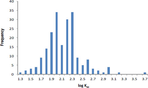
FIGURE 3-1 Organic-carbon normalized sorption coefficients, Koc, values for atrazine plotted on a logarithmic scale. Source: Gerstl 1990. Reprinted with permission; copyright 1990, Journal of Contaminant Hydrology.
FIGURE 3-2 Distribution of Koc values for atrazine in a 6.25 hectare field, showing a range of about a factor of 2. Source: Novak et al. 1997. Reprinted with permission; copyright 1997, Journal of Environmental Quality.
Perhaps more important, larger inaccuracies in predicting the amount of chemical sorbed to soil or sediment particles will result if the model used to describe the sorption process is inaccurate. For example, one cannot expect an accurate result if one uses a sorption model designed for nonionic pesticides (Kd = focKoc) when modeling ionic compounds. Some modelers made that mistake with the herbicide 2, 4-D, which typically exists in water as a negatively charged species. A modeler should expect its sorption to involve anion exchange, as has been shown by Hyun and Lee (2005). A second case of an inappropriate use of the focKoc model involves situations in which black carbon sorbents play an important role in addition to the rest of the organic carbon. Yang and Sheng (2003) have provided evidence of such sorption to black carbon in the case of diuron applied to a field with burned wheat and rice residues. Thus, although cases that accurately use the focKoc model probably reflect modest levels of uncertainty (1 SD, reflecting a factor of 2-4), pesticide-fate modelers should recognize both chemical-specific properties and site-specific conditions that can cause their estimates of sorption to be quite inaccurate—not merely imprecise but biased by a factor of 10—when such a sorption model is inappropriately used (Accardi-Dey and Gschwend 2002).
Even the best estimates of biodegradation coefficients are generally much more uncertain than sorption estimates. When Laskowski (1995) reviewed literature on biodegradation rates in soils, he found that for many chemicals few soils were tested (Table 3-2). However, when substantial data were available, biodegradation rates varied widely, often by more than a factor of 10 (Table 3-2). Likewise, Paris et al. (1981) found that the rates of biohydrolysis of the butoxyethyl ester of 2, 4-D varied by up to a factor of 25 in 33 water samples tested even when efforts were made to account for sample-to-sample variations in microbial population densities. Finally, in some cases, such as nitrilotriacetate, Tiedje and Mason (1974) observed significant lag periods (4-6 days) in three of 11 soils tested. Thus, inaccuracies will result if a simple first-order removal-rate law with a single-value rate coefficient is used for periods that are shorter than or comparable with such lag periods.
TABLE 3-2 Variability of Pesticide Degradation Rates in Soils
| Pesticide | No. Soils Tested | Ratio of Highest to Lowest Degradation Rate Observed | Reference |
| Nitrilotriacetate | 11 | 80 | Tiedje and Mason 1974 |
| Crotoxyphos | 3 | 36 | Konrad and Chesters 1969 |
| Carbofuran | 4 | 25 | Getzin 1973 |
| Glyphosate | 4 | 19 | Rueppel et al. 1977 |
| Flumetsulam | 21 | 10 | Lehmann et al. 1992 |
| Chlorimuron ethyl | 19 | 8 | L.M. Kennard and D.A. Laskowski, DowElanco, unpublished material, 1992 |
| Thionazin | 4 | 7 | Getzin and Rosefield 1966 |
| Nitrapyrin | 10 | 6 | Laskowski and Regoli 1972 |
| Imazaquin | 3 | 5 | Basham and Lavy 1987 |
| Chlorsulfuron | 8 | 4 | Walker et al. 1989 |
| Methidathion | 4 | 3 | Getzin 1970 |
| Aldicarb | 2 | 2 | Richey et al. 1977 |
| Diazinon | 4 | 2 | Getzin and Rosefield 1966 |
| Linuron | 4 | 2 | Lode 1967 |
| Methomyl | 2 | 2 | Harvey and Pease 1973 |
| Propyzamide | 5 | 2 | Walker 1976 |
Source: Adapted from Laskowski et al. 1982; Laskowski 1995.
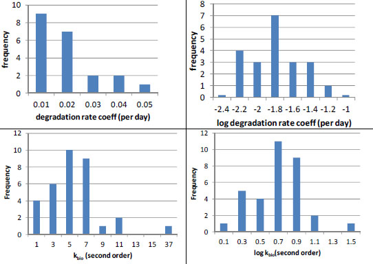
In the few cases in which sufficient data are available, it appears that biodegradation rates are log-normally distributed (Figure 3-3). For example, the (pseudo-) first-order rate coefficients reported by Lehmann et al. (1992) for flumetsulam appear to have a log-normal distribution (Figure 3-3, N = 21). Paris et al. (1981) also found that the microbial population-normalized rate coefficients appeared to be log-normally distributed with a kbio value of about 100.7 ± 0.3 L/colony forming units (cfu) per hour (10mean ± 1SD, N = 33) for biohydrolysis of the butoxyethyl ester of 2, 4-D. In both cases, the data suggest uncertainty of about a factor of 2 (about ±0.3 log units around the mean). To summarize, pesticide-exposure analysis should be pursued by using enough biotransformation information to establish whether the rates are normally or log-normally distributed, and then the data should be analyzed to obtain the mean rate coefficient and its variance for use in fate modeling.
It is also clear that rates of biodegradation of some pesticides can vary widely as a function of site conditions. As stated by Howard (1991) in discussing 2, 4-D in surface waters,
the rate will depend on a number of factors including presence of acclimated organisms, nutrient levels, temperature and concentration of 2, 4-D. Half-lives in river water of 18 to over 50 days (clear water) and 10 to 25 days (muddy water) with lag times of 6 to 12 days have been reported.… Degradation is poor in oligotrophic water and where high 2, 4-D concentrations are present and 2, 4-D was not mineralized in water from 2 or 3 lakes tested.
Clearly, environmental conditions (such as temperature and oxic or anoxic conditions in soil or sediment), nutrient availability, and factors controlling pesticide speciation (dissolved vs sorbed) can greatly affect biodegradation. Perhaps the general uncertainty in biodegradation rates is best captured in the tendency of some investigators to refer simply to individual pesticides as “non-persistent,” “moderately persistent,” and “highly persistent.” For example, Corbin et al. (2004) describe 2, 4-D as “non-persistent” (t1/2 = 6.2 days) in terrestrial environments, “moderately persistent” (t1/2 = 45 days) in aerobic aquatic environments, and “highly persistent” (t1/2 = 231 days) in anaerobic terrestrial and aquatic systems.
An Example of Current Modeling Input Choices in the Face of Parameter Uncertainty
To understand the approaches being used to account for uncertainty in modeling parameters, one can consider how biodegradation information was used in a PRZM-EXAM analysis of the ethyl hexyl ester (EHE) of 2, 4-D (see Table 3-3). The compound is a nonionic ester, is quite hydrophobic, and thus is
highly sorptive (Koc about 10,500). In a typical soil with an organic carbon content near 1%, one expects a sorption coefficient near 100 L/kg. That value means that almost all the ester (over 99%) is sorbed and somewhat unavailable to microorganisms. The extensive sorption implies that soil-to-soil differences in organic carbon content will affect the ester's bioavailability correspondingly and change the biodegradation rate accordingly. For example, soil with 3% organic carbon content will limit this ester's bioavailability by a factor of 3 relative to soil with 1% organic carbon content.
Next, the aerobic soil metabolism rate listed in Table 3-3 is based on a single soil-volatility study in which the ester was seen to degrade with a half-life of 8 days. Clearly, that information is not enough to provide any sense of the statistical variability in the biodegradation rate. Consequently, Corbin et al. (2004) compensated by providing some margin of safety, cutting the rate by a factor of 3 to arrive at a half-life of 24 days in aerobic soil. However, no scientific justification for a factor of 3 is provided; such a choice would require more observations. Furthermore, as directed in the modeling guidance (see Footnote b of Table 3-3), the aerobic aquatic degradation rate was set to half the value used for the aerobic soil case, yielding a half-life of 48 days. In the absence of any data, the guidance also leads one to assume that the ethylhexyl ester of 2, 4-D is “stable” in anaerobic medias, such as sediments. Given those somewhat arbitrary inputs, PRZM/EXAM proceeds to estimate environmental concentrations of 2, 4-D EHE. The approach leaves no possibility of assessing the probability distributions of the resultant EECs. The outcome of the model is quantitative, but its accuracy and precision are unknown.
Quantifying Parameter Uncertainty
It is clear from the above discussion that input parameters for fate and transport models have several components of uncertainty, including differences associated with environmental variability, imprecision of measurements under natural conditions, and lack of knowledge (see Chapter 2). Therefore, use of single values in a deterministic modeling approach provides an unwarranted sense of accuracy in predicting pesticide fate and later concentrations in water or loading on sediments and soils. As discussed in Chapter 2, the committee recommends taking a probabilistic approach and assigning appropriate distributions to the input parameters instead of single values. The committee notes that EPA has been working on probabilistic exposure modeling for many years (see, for example, Burns 2001). Model runs can be done with Monte Carlo techniques as single-level or multilevel models. The output is then a range of possible environmental concentrations with their associated probabilities of occurrence. That approach provides the required input information for comparison with hazard function to provide a probabilistic risk estimate.
| Model Parameter | Value | Comments | Source |
| Aerobic soil metabolism, t½ | 24 daysa | Estimated upper 90th percentile | MRID 42059601 |
| Aerobic aquatic degradation, t½ (KBACW) | 48 days | Half the aerobic soil metabolism degradation rate | Estimated per EFED Guidanceb |
| Anaerobic aquatic degradation, t½ (KBACS) | Stable | No data | Estimated per EFED Guidance2 |
| Aqueous photolysis, t½ | 128 days | MRID 42749702 | |
| Hydrolysis, t½ | 48 days | MRID 42735401 | |
| Koc | 10,500 mL/g | Estimated by EpiSuite Software | |
| Molecular weight | 333.26 | Product Chemistry | |
| Water solubility | 0.32 mg/L | Product Chemistry | |
| Vapor pressure | 4.57 E-6 mm Hg | Product Chemistry | |
| Henry’s law constant | 5.78 E-5 atm-m3/mole | Product Chemistry | |
aThree times (upper 90th percentile) based on single soil half-life estimated from acceptable laboratory volatility study of 8 days.
bFrom Guidance for Chemistry and Management Practice Input Parameters for Use in Modeling the Environmental Fate and Transport of Pesticides, dated February 28, 2002.
Abbreviations: EFED, Environmental Fate and Effects Division of EPA; KBACS, first-order rate constant for pesticide’s bacterial degradation in sediment (day-1); KBACW, first-order rate constant for pesticide’s bacterial degradation in water (day-1); MRID, master record identification number (a unique cataloging number assigned to an individual pesticide study at the time of its submission to the agency).
Source: Corbin et al. 2004.
Interdependence of Input Parameters
Intervariable dependence can result in large uncertainty in model output, particularly when probabilistic modeling techniques are used. Assuming that all variables in an assessment are mutually independent will lead to erroneous risk results that might be conservative. That situation occurs whether the distributions characterizing the several variables represent natural variability or lack of information. Correctly modeling dependences usually requires additional empirical information beyond means, dispersions, and marginal distributions of input
parameters and requires special modeling and mathematical techniques to propagate dependence. It seems unlikely that all input parameters are independent or perfectly dependent; these are the cases for which relatively simple solutions exist. However, the complexities of modeling incomplete dependence of multiple model parameters (Ferson et al. 2004; Kurowicka and Cooke 2006) probably outweigh the increased precision of the models. Therefore, for regulatory purposes, including ESA consultations, the committee recommends continuing to use the simplifying assumption of independence of model input parameters and to acknowledge the residual uncertainties of such an approach.
CONCLUSIONS AND RECOMMENDATIONS
Exposure-Modeling Practices
• Although the mass-balance models have many strengths, model limitations need to be recognized, and the appropriate model needs to be used for different risk-assessment contexts. Accordingly, a screening-level model should not be used when a refined exposure analysis is needed, such as in Step 2 or 3 assessments in the ESA process.
• To estimate pesticide exposure concentrations at various stages, the committee proposes a stepwise approach to exposure modeling. Step 1 would determine whether a pesticide and listed species overlap geographically and temporally. Step 2 would first identify the most important fate processes and other related considerations and then simplify the pesticide-fate model to estimate time-varying and space-varying pesticide concentrations in generic habitats relevant to the listed species. Step 3 would use refined models and the regional-specific or site-specific input values relevant to the listed species.
• Field studies need to be distinguished from general monitoring studies that are not associated with specific pesticide applications under well-described conditions. The latter cannot be used to estimate pesticide concentrations after a pesticide application or to evaluate model performance.
• Model predications are only as accurate or precise as parameter information. Thus, key processes need to be identified and the associated parameter values well defined.
Geospatial Data
• Although data on species occurrence inevitably are incomplete, uncertainties in modeled distributions of species typically can be quantified, and statistical characterizations of species distributions, species-environment relations, and the location and quality of habitat are more objective and reliable than qualitative descriptions of habitat.
• Existing and authoritative geospatial data on many scales are sufficient to support a substantial majority of habitat delineations and exposure analyses under the ESA and FIFRA. Widely recognized sources of data on environmental attributes—including topography, hydrography, meteorology, solar radiation, soils, geology, and land cover—can be used reliably for modeling species distributions and chemical fate. The authoritative sources that are most useful will vary among species and pesticides.
• Use of data and metadata that comply with the National Spatial Data Infrastructure can increase the clarity and repeatability of data analysis; facilitate quantification or even reduction of uncertainties in analytical results; and improve communication.
Uncertainties
• Any exposure analysis involving pesticide applications should at least qualitatively describe the potential effect of inerts on the environmental fate of an active ingredient. If the available information suggests that inerts (or adjuvants) might substantially affect the fate or transport of an active ingredient, the effect should be assessed quantitatively if data to support such a consideration are available.
• The extent to which the environmental fate of inerts or adjuvants needs to be considered quantitatively will depend largely on toxicological considerations (see Chapter 4). In the absence of information on the environmental-fate properties of inerts or adjuvants, quantitative structure-activity relationships can be used to estimate fate properties, but the use of such estimates will add to the uncertainties in the exposure analysis.
• Ideally, any risk assessment or BiOp should be based on exposures to pesticide components and other chemical agents that will occur in the field. Nonetheless, few methods are available for assessing exposure to environmental mixtures quantitatively or for predicting the relative concentrations of different mixture components in various environmental media, especially water and sediments. Monitoring data on the pesticides and other stressors will provide information about what is occurring in a specific area of concern but are not useful for model comparisons.
• In the absence of quantitative estimates of exposure, assessors should exclude potential mixture components from quantitative assessments. Uncertainties associated with the identities or exposure concentrations of potential mixture constituents should be qualitatively described to a decision-maker.
• Many diverse parameters are used in chemical-fate models, and their accuracy is important ultimately for the concentrations estimated in modeling efforts. However, little effort has been expended to evaluate the date inputs relevant to particular ESA evaluations. Therefore, if the agencies want to obtain more accurate modeling results, a subset of case-specific exposure estimates
should be evaluated by pursing a measurement campaign specifically coordinated with several pesticide field applications.
• Sorption and biodegradation are important chemical-fate processes that are often associated with substantial uncertainty or represented inaccurately in fate models. More sorption data are needed to characterize nonlinear isotherms over concentration ranges and under conditions that are applicable to relevant agricultural settings, such as pH, ionic composition, and solid-phase mineralogy. Likewise, more data are needed to determine biodegradation coefficients, whether biodegradation rates are normally or log-normally distributed, and under which circumstances lag periods are important.
Accardi-Dey, A.M., and P.M. Gschwend. 2002. Assessing the combined roles of natural organic matter and black carbon as sorbents in sediments. Environ. Sci. Technol. 36(1):21-29.
Araújo, M.B., and R.G. Pearson. 2005. Equilibrium of species’ distributions with climate. Ecography 28(5):693-695.
ATSDR (Agency for Toxic Substances and Disease Registry). 1999. Toxicological Profile for Total Petroleum Hydrocarbons (TPH). U.S. Department of Health and Human Services, Public Health Service, Agency for Toxic Substances and Disease Registry, Atlanta, GA. September 1999 [online]. Available: http://www.atsdr.cdc.gov/ToxProfiles/tp.asp?id=424&tid=75 [accessed Feb. 25, 2012].
Basham, G.W., and T.L. Lavy. 1987. Microbial and photolytic dissipation of imazaquin in soil. Weed Sci. 35(6):865-870.
Beestman, G.B. 1996. Emerging technology: The bases for new generations of pesticide formulations. Pp. 43-68 in Pesticide Formulation and Adjuvant Technology, C.L. Foy, and D.W. Pritchard, eds. Boca Raton, FL: CRC Press.
Belden, J.B., R.J. Gilliom, J.B. Martin, and M.J. Lydy. 2007. Relative toxicity and occurrence patterns of pesticide mixtures in streams draining agricultural watersheds dominated by corn and soybean production. Integr. Environ. Assess. Manag. 3(1): 90-100.
Bird, S.L., S.G. Perry, S.L. Ray, and M.E. Teske. 2002. Evaluation of the AgDISP aerial spray algorithms in the AgDRIFT model. Environ. Toxicol. Chem. 21(3):672-681.
Boyce, M.S., P.R. Vernier, S.E. Nielsen, and F.K.A. Schmiegelow. 2002. Evaluating resource selection functions. Ecol. Model. 157(2-3):281-300.
Bradbury, R.B., R.A. Hill, D.C. Mason, S.A. Hinsley, J.D. Wilson, H. Balzter, G.Q.A. Anderson, M.J. Whittingham, I.J. Davenport, and P.E. Bellamy. 2005. Modeling relationships between birds and vegetation structure using airborne LiDAR data: A review with case studies from agricultural and woodland environments. Ibis 147(3): 443-452.
Brausch, J.M., and P.N. Smith. 2007. Toxicity of three polyethoxylated tallowamine surfactant formulations to laboratory and field collected fairy shrimp, Thamnocephalus platyurus. Arch. Environ. Contam. Toxicol. 52(2):217-221.
Buckland, S.T., D.R. Anderson, K.P. Burnham, J.L. Laake, D.L. Borchers, and L. Thomas. 2001. Introduction to Distance Sampling: Estimating Abundance of Biological Populations. New York: Oxford University Press.
Burns, L.A. 2001. Probabilistic Aquatic Exposure Assessment for Pesticides, 1. Foundations. EPA/600/R-01/071. U.S. Environmental Protection Agency, Washington, DC. September 2001.
Burns, L.A. 2004. Exposure Analysis Modeling System (EXAMS): User Manual and System Documentation. EPA/600/R-00/081, Revision G. National Exposure Research Laboratory, Office of Research and Development, U.S. Environmental Protection Agency, Washington, DC. May 2004 [online]. Available: http://www.epa.gov/ceampubl/swater/exams/exams29804/EXAMREVG.PDF [accessed Nov. 16, 2012].
Burns, L.A. 2006. User Manual for EXPRESS, the “EXAMS-PRZM Exposure Simulation Shell”. EPA/600/R-06/095. NTIS PB2007-100140. Office of Research and Development, U.S. Environmental Protection Agency, Washington, DC. September 2006 [online]. Available: http://www.epa.gov/ceampubl/swater/express/Express.pdf [accessed Nov. 16, 2012].
CA Department of Conservation. 2007a. Farmland Mapping & Monitoring Program [online]. Available: http://www.conservation.ca.gov/dlrp/fmmp/Pages/Index.aspx [accessed Nov. 14, 2012].
CA Department of Conservation. 2007b. Farmland Mapping & Monitoring Program-Important Farmland Map Categories [online]. Available: http://www.conservation.ca.gov/dlrp/fmmp/mccu/Pages/map_categories.aspx [accessed Nov. 14, 2012].
Clevenger, A.P., J. Wierzchowski, B. Chruszcz, and K.E. Gunson. 2002. GIS-generated, expert-based models for identifying wildlife habitat linkages and planning mitigation passages. Conserv. Biol. 16(2):503-514.
Corbin, M., W. Evans, and J. Hetrick. 2004. Environmental Fate and Effects Division's Risk Assessment for the Reregistration Eligibility Document for 2, 4-Dichlorophenoxyacetic Acid (2, 4-D). U.S. Environmental Protection Agency [online]. Available: http://www.epa.gov/espp/litstatus/effects/24d/attachment-b.pdf [accessed Sept. 4, 2012].
DCMI (Dublin Core Metadata Initiative Limited). 2012. Metadata Basic [online]. Available: http://dublincore.org//metadata-basics/ [accessed Nov. 14, 2012].
Denis, M.H., and S. Delrot. 1997. Effects of salts and surfactants on foliar uptake and long distance transport of glyphosate. Plant Physiol. Biochem. 35(4):291-301.
Dickson, B.G., and P. Beier. 2007. Quantifying the influence of topographic position on cougar (Puma concolor) movement in southern California, USA. J. Zool. 271(3): 270-277.
Dragovich, J.D., R.L. Logan, H.W. Schasse, T.J. Walsh, W.S. Lingley, Jr., D.K. Norman, W.J. Gerstel, T.J. Lapen, J.E. Schuster, and K.D. Meyers. 2002. Geologic Map of Washington-Northwest Quadrant. Geologic Map GM-50. Washington State Department of Natural Resources [online]. Available: http://www.dnr.wa.gov/Publications/ger_gm50_geol_map_nw_wa_250k.pdf [accessed Nov. 14, 2012].
Effland, W.R., N.C. Thurman, and I. Kennedy. 1999. Proposed Methods For Determining Watershed-Derived Percent Cropped Areas and Considerations for Applying Crop Area Adjustments To Surface Water Screening Models. Presentation To FIFRA Science Advisory Panel, May 27, 1999 [online]. Available: http://www.epa.gov/scipoly/sap/meetings/1999/may/pca_sap.pdf [accessed Mar. 13, 2013].
Elith, J., C.H. Graham, R.P. Anderson, M. Dudik, S. Ferrier, A. Guisan, R.J. Hijmans, F. Huettmann, J.R. Leathwick, A. Lehmann, J. Li, L.G. Lohmann, B.A. Loiselle, G. Manion, C. Moritz, M. Nakamura, Y. Nakazawa, J.M. Overton, T.A. Peterson, S.J. Phillips, K. Richardson, R. Scachetti-Pereira, R.E. Schapire, J. Soberon, S. Williams, M.S. Wisz, and N.E. Zimmermann. 2006. Novel methods improve prediction of species distributions from occurrence data. Ecography 29(2):129-151.
EPA (U.S. Environmental Protection Agency). 1993. Wildlife Exposure Factors Handbook. EPA/600/R-93/197. Office of Research and Development, U.S. Environmental Protection Agency, Washington, DC [online]. Available: http://cfpub.epa.gov/ncea/cfm/recordisplay.cfm?deid=2799#Download [accessed Mar. 11, 2013].
EPA (U.S. Environmental Protection Agency). 2001. GENEEC (Generic Estimated Environmental Concentrations): Development and Use of GENEEC Version 2.0 for Pesticides, Aquatic Ecological Exposure Assessment, May 1, 2001. Environmental Fate and Effects Division, Office of Pesticide Programs, U.S. Environmental Protection Agency, Washington, DC [online]. Available: http://www.epa.gov/oppefed1/models/water/geneec2_description.htm [accessed Mar. 13, 2013].
EPA (U.S. Environmental Protection Agency). 2010. Label Review Manual [online]. Available: http://www.epa.gov/oppfead1/labeling/lrm/ [accessed Nov. 12, 2012].
EPA (U.S. Environmental Protection Agency). 2011. Inert Ingredients Permitted for Use in Nonfood Use Pesticide Products. Office of Prevention, Pesticides, and Toxic Substances, U.S. Environmental Protection Agency, Washington, DC. April 2011 [online]. Available: http://www.epa.gov/opprd001/inerts/inert_nonfooduse.pdf [accessed Nov. 12, 2012].
EPA (U.S. Environmental Protection Agency). 2012a. Technical Overview of Ecological Risk Assessment Risk Characterization. U.S. Environmental Protection Agency [online]. Available: http://www.epa.gov/oppefed1/ecorisk_ders/toera_risk.htm [accessed Mar. 22, 2013].
EPA (U.S. Environmental Protection Agency). 2012b. PRZM Version Index. Exposure Assessment Models Groundwater, U.S. Environmental Protection Agency [on-line]. Available: http://www.epa.gov/ceampubl/gwater/przm3/ [accessed Nov. 14, 2012].
EPA (U.S. Environmental Protection Agency). 2012c. EXAMS Version Index. Exposure Assessment Models Surface Water, U.S. Environmental Protection Agency [on-line]. Available: http://www.epa.gov/ceampubl/swater/exams/ [accessed Nov. 14, 2012].
EPA (U.S. Environmental Protection Agency). 2012d. Terrestrial Models. U.S. Environmental Protection Agency [online]. Available: http://www.epa.gov/oppefed1/models/terrestrial/ [accessed Mar. 22, 2013].
EPA (U.S. Environmental Protection Agency). 2012e. Surf Your Watershed. U.S. Environmental Protection Agency [online]. Available: http://cfpub.epa.gov/surf/locate/index.cfm [accessed Feb. 29, 2012).
EPA (U.S. Environmental Protection Agency). 2012f. GCSOLAR. Exposure Assessment Models Surface Water, U.S. Environmental Protection Agency [online]. Available: http://www.epa.gov/ceampubl/swater/gcsolar/ [accessed Nov. 14, 2012].
EPA (U.S. Environmental Protection Agency). 2012g. Pesticide Inert ingredients [online]. Available: http://www.epa.gov/opprd001/inerts/[accessed Nov. 14, 2012].
EPA (U.S. Environmental Protection Agency). 2012h. InertFinder [online]. Available: http://iaspub.epa.gov/apex/pesticides/f?p=901:1:1130545917893601 [accessed Nov. 16, 2012].
EPA (U.S. Environmental Protection Agency). 2012i. EPA Response to NAS Questions, March 28, 2012 [online]. Available: http://www.thecre.com/forum1/wp-content/uploads/2012/04/ESAEPAATRAZINE.pdf [accessed Nov. 15, 2012].
ESRI. 2010. Topography Tools for ArcGIS (9.3, 9.2, 9.1/9.0). ESRI, Redlands, CA [online]. Available: http://arcscripts.esri.com/details.asp?dbid=15996 [accessed Nov. 14, 2012].
ESRL (Earth System Research Laboratory). 2012. PSD Gridded Climate Datasets. National Oceanic and Atmospheric Administration, Earth System Research Laboratory [online]. Available: http://www.esrl.noaa.gov/psd/data/gridded/ [accessed Nov. 14, 2012].
Ferrell, J.A., G.E. MacDonald, and B. Sellers. 2008. Adjuvants. Document SS-AGR-109. Electronic Data Information Source (EDIS), University of Florida (UF), Institute of Food and Agricultural Sciences (IFAS) [online]. Available: http://edis.ifas.ufl.edu/wg050 [accessed Feb. 26, 2012].
Ferson, S., R.B. Nelsen, J. Hajagos, D.J. Berleant, J. Zhang, W.T. Tucker, L.R. Ginzburg, and W.L. Oberkamp. 2004. Dependence in Probabilistic Modeling, Dempster-Shafer Theory, and Probability Bounds Analysis. SAND2004-3072. Sandia National Laboratories, Albuquerque, NM [online]. Available: http://www.ramas.com/depend.pdf [accessed Mar. 25, 2013].
FGDC (Federal Geographic Data Committee). 2007. National Spatial Data Infrastructure [online]. Available: http://www.fgdc.gov/nsdi/nsdi.html [accessed Mar. 7, 2012].
FGDC (Federal Geographic Data Committee). 2012. Geospatial Metadata. What are Metadata? [online]. Available: http://fgdc.gov/metadata [accessed Nov. 14, 2012].
Fletcher, J.S., J.E. Nellesson, and T.G. Pfleeger. 1994. Literature review and evaluation of the EPA food-chain (Kenaga) nomogram, an instrument for estimating pesticide residues on plants. Environ. Toxicol. Chem. 13(9):1383-1391.
Franklin, J. 2009. Mapping Species Distributions: Spatial Inference and Prediction. Cambridge, UK: Cambridge University Press.
Fretwell, S.D. 1972. Populations in a Seasonal Environment. Princeton, NJ: Princeton University Press.
Gerstl, Z. 1990. Estimation of organic chemical sorption by soils. J. Contam. Hydrol. 6(4): 357-375.
Getzin, L.W. 1970. Persistence of methidathion in soils. Bull. Environ. Contam Toxicol. 5(2):104-110.
Getzin, L.W. 1973. Persistence and degradation of carbofuran in soils. Environ. Entomol. 2(3):461-468.
Getzin, L.W., and I. Rosefield. 1966. Persistence of diazinon and zinophos in soils. J. Econ. Entomol. 59(3):512-516.
Gilliom, R.J., J.E. Barbash, C.G. Crawford, P.A. Hamilton, J.D. Martin, N. Nakagaki, L.H. Nowell, J.C. Scott, P.E. Stackelberg, G.P. Thelin, and D.M. Wolock. 2007. The Quality of Our Nation's Waters: Pesticides in the Nation's Streams and Groundwater, 1992-2001. U.S. Geological Survey Circular 1291. U.S. Geological Survey, Reston, VA [online]. Available: http://pubs.usgs.gov/circ/2005/1291/pdf/circ1291.pdf [accessed Nov. 13, 2012].
Hall, L.S., P.R. Krausman, and M.L. Morrison. 1997. The habitat concept and a plea for standard terminology. Wildl. Soc. Bull. 25(1):173-182.
Han, W., Z. Yang, L. Di, and R. Mueller. 2012. CropScape: A Web service based application for exploring and disseminating U.S. conterminous geospatial cropland data products for decision support. Comput. Electron. Agr. 84:111-123.
Harvey, J., Jr., and H.L. Pease. 1973. Decomposition of the methomyl in soil. J. Agric. Food Chem. 21(5):784-786.
Hoerger, F., and E.E. Kenaga. 1972. Pesticide residues on plants: Correlation of representative data as a basis for estimation of their magnitude in the environment. Pp. 9-28 in Environmental Quality and Safety: Chemistry, Toxicology, and Technology, Vol. 1. Global Aspects of Chemistry, Toxicology, and Technology as Applied
to the Environment, F. Coulston, and F. Korte, eds. Stuttgart: Georg Thieme Verlag.
Hoogeweg, C.G., W.M. Williams, R. Breuer, D. Denton, B. Rook, and C. Watry. 2011. Spatial and Temporal Quantification of Pesticide Loadings to the Sacramento River, San Joaquin River, and Bay-Delta to Guide Risk Assessment for Sensitive Species. CALFED Science Grant No. 1055. Waterborne Environmental, Inc., Leesburg, VA, and University of California, Davis, CA. November 2, 2011. 293 pp [online]. Available: http://www.waterborne-env.com/publications/papers_reports/CALFED_Final_Report_2011-Nov_2.pdf [accessed on May 9, 2012].
Hope, B.K. 2012. Using legacy data to relate biological condition to cumulative aquatic toxicity in the Willamette River Basin (Oregon, USA). Arch. Environ. Contam. Toxicol. 62(3):424-437.
Horning, N., J.A. Robinson, E.J. Sterling, W. Turner, and S. Spector. 2010. Remote Sensing for Ecology and Conservation: Handbook of Techniques. New York: Oxford University Press.
Howard, P.H., ed. 1991. 2, 4-D. Pp. 145-156 in Handbook of Environmental Fate and Exposure Data for Organic Chemicals. Boca Raton, FL: CRC Press.
Hyun, S., and L.S. Lee. 2005. Quantifying the contribution of different sorption mechanisms for 2, 4-dichlorophenoxyacetic acid sorption by several variable-charge soils. Environ. Sci. Technol. 39(8):2522-2528.
Jenness Enterprises. 2011. DEM Surface Tools. Jenness Enterprises, Flagstaff, AZ [online]. Available: http://www.jennessent.com/arcgis/surface_area.htm [accessed Nov. 14, 2012].
Karl, H.A., L.E. Susskind, and K.H. Wallace. 2007. A dialogue, not a diatribe: Effective integration of science and policy through joint fact finding. Environment 49(1):20-34.
Katagi, T. 2008. Surfactant effects on environmental behavior of pesticides. Rev. Environ. Contam. Toxicol. 194:71-177.
Knisel, W.G., and F.M. Davis. 2000. GLEAMS (Groundwater Loading Effects of Agricultural Management Systems), Version 3.0, User Manual. Publication No. SEWRLWGK/FMD-050199. U.S. Department of Agriculture, Agricultural Research Service, Southeast Watershed Research Laboratory, Tifton, GA. August 15, 2000. 194pp.
Konrad, J.G., and G. Chesters. 1969. Degradation in soil of ciodrin, an organophosphate insecticide. J. Agric. Food Chem. 17(2):226-230.
Kosswig, K. 1994. Surfactants. Pp. 747-815 in Ullmann’s Encyclopedia of Industrial Chemistry, Vol. 25A, Starch and Other Polysaccharides to Surfactants, 5th Ed. Weinheim: Wiley-VCH.
Kurowicka, D., and R.M. Cooke. 2006. Uncertainty Analysis with High Dimensional Dependence Modeling. Hoboken, NJ: John Wiley & Sons Inc.
Laskowski, D.A. 1995. EPA guidelines for environmental fate studies: Meaningful data for assessing exposure to pesticides. Pp. 117-128 in Agrochemical Environmental Fate: State of the Art, M.L. Leng, E.M.K. Leovey, and P.P. Zubkoff, eds. New York: Lewis.
Laskowski, D.A., and A.J. Regoli. 1972. Influence of the environment on N-SERVE stability. Agron. Abstacts 97 (as cited in Laskowski 1995).
Laskowski, D.A., C.A.I. Goring, P.J. McCall, and R.L. Swann. 1982. Terrestrial environment. Pp.198-240 in Environmental Risk Analysis for Chemicals, R.C. Conway, ed. New York: Van Nostrand Reinhold.
Lehmann, R.G., J.R. Miller, D.D. Fontaine, D.A. Laskowski, J.H. Hunter, and R.C. Cordes. 1992. Degradation of a sulfonamide herbicide as a function of soil sorption. Weed Res. 32(3):197-205.
Leonard, R.A., W.G. Knisel, and D.A. Still. 1989. GLEAMS: Groundwater loading effects of agricultural management systems. Transactions ASAE. 30:1403-1418.
Lin, K., D. Haver, L. Oki, and J. Gan. 2009. Persistence and sorption of fipronil degradates in urban stream sediments. Environ. Toxicol. Chem. 28(7):1462-1468.
Liu, Z. 2004. Effects of surfactants on foliar uptake of herbicides - a complex scenario. Colloids Surf. B Biointerfaces 35(3-4):149-153.
Loague, K., and R.E. Green. 1991. Statistical and graphical methods for evaluating solute transport models: Overview and application. J. Contam. Hydrol. 7:51-73.
Lode, O. 1967. Decomposition of linuron in different soils. Weed Res. 7(3):185-190.
MacKenzie, D.I., J.D. Nichols, J.A. Royle, K.H. Pollock, L.L. Bailey, and J.E. Hines. 2006. Occupancy Estimation and Modeling: Inferring Patterns and Dynamics of Species Occurrence. San Diego, CA: Academic Press.
Manly, B.F., L. McDonald, D.L. Thomas, T.L. MacDonald, and W.P. Erickson. 2010. Resource Selection by Animals: Statistical Design and Analysis for Field Studies, 2nd Ed. Dordrecht, the Netherlands: Kluwer.
Martinuzzi, S., L.A. Vierling, W.A. Gould, M.J. Falkowski, J.S. Evans, A.T. Hudak, and K.T. Vierling. 2009. Mapping snags and understory shrubs for a LiDAR-based assessment of wildlife habitat suitability. Remote Sens. Environ. 113(12):2533-2546.
Mitchell, S.C. 2005. How useful is the concept of habitat? A critique. Oikos 110(3):634-638.
Morrison, M.L., and L.S. Hall. 2002. Standard terminology: Toward a common language to advance ecological understanding and application. Pp. 43-52 in Predicting Species Occurrences: Issues of Accuracy and Scale, J.M. Scott, P.J. Heglund, M.L. Morrison, J.B. Haufler, M.G. Raphael, W.A. Wall, and F.B. Samson, eds. Covelo, CA: Island Press.
NASS (National Agricultural Statistics Service). 2010. Charts and Maps. U.S. Department of Agriculture, National Agricultural Statistics Service [online]. Available: http://www.nass.usda.gov/Charts_and_Maps/index.asp [accessed Nov. 14, 2012].
Nagy, K.A., and C.C. Peterson. 1988. Scaling of Water Flux Rates in Animals. Berkeley, CA: University of California Press.
NCDC (National Climatic Data Center). 2012. NOAA Regional Climate Centers [online]. Available: http://www.ncdc.noaa.gov/oa/climate/regionalclimatecenters.html [accessed Nov. 14, 2012].
NMFS (National Marine Fisheries Service). 2008. Biological Opinion, Environmental Protection Agency Registration of Pesticides Containing Chlorpyrifos, Diazinon, and Malathion. National Marine Fisheries Service, Silver Spring, MD. November 18, 2008 [online]. Available: http://www.nmfs.noaa.gov/pr/pdfs/pesticide_biop.pdf [accessed Nov. 13, 2012].
NMFS (National Marine Fisheries Service). 2009. Biological Opinion, Endangered Species Act Section 7 Consultation, Environmental Protection Agency Registration of Pesticides Containing Carbaryl, Carbofuran, and Methomyl. National Marine Fisheries Service, Silver Spring, MD. April 20, 2009 [online]. Available: http://www.nmfs.noaa.gov/pr/pdfs/carbamate.pdf [accessed Nov. 12, 2012].
NMFS (National Marine Fisheries Service). 2010. Biological Opinion, Endangered Species Act Section 7 Consultation, Environmental Protection Agency Registration of Pesticides Containing Azinphos methyl, Bensulide, Dimethoate, Disulfoton, Ethoprop, Fenamiphos, Naled, Methamidophos, Methidathion, Methyl parathion, Phor-
ate and Phosmet. National Marine Fisheries Service, Silver Spring, MD. August 31, 2010 [online]. Available: http://www.nmfs.noaa.gov/pr/pdfs/final_batch_3_opinion.pdf [accessed Nov. 13, 2012].
NMFS (National Marine Fisheries Service). 2011. Biological Opinion, Endangered Species Act Section 7 Consultation, Environmental Protection Agency Registration of Pesticides 2, 4-D, Triclopyr BEE, Diuron, Linuron, Captan, and Chlorothalonil. National Marine Fisheries Service, Silver Spring, MD. June 30, 2011 [online]. Available: http://www.nmfs.noaa.gov/pr/pdfs/consultations/pesticide_opinion4.pdf [accessed Nov. 13, 2012].
Noon, B.R. 1981. Techniques for sampling avian habitats. Pp. 42-52 in The Use of Multivariate Statistics in Studies of Wildlife Habitat, D.E. Capen, ed. General Technical Report RM-89. U. S. Forest Service, Rocky Mountain Forest and Range Experimental Station, Fort Collins, CO [online]. Available: http://fishwild.vt.edu/Chihuahua%202005/READINGS/noon.pdf [accessed Nov. 13, 2012].
Novak, J.M., T.B. Moorman, and C.A. Cambardella. 1997. Atrazine sorption at the field scale in relation to soils and landscape position. J. Environ. Qual. 26(5):1271-1277.
NRC (National Research Council). 1993. Toward a Coordinated Spatial Data Infrastructure for the Nation. Washington, DC: National Academy Press.
NRCS (National Resource Conservation Service). 2012a. Watershed Boundary Data Set [online]. Available: http://www.nrcs.usda.gov/wps/portal/nrcs/main/national/water/watersheds/dataset [accessed Feb. 29, 2012].
NRCS (National Resource Conservation Service). 2012b. Web Soil Survey (WSS) [online]. Available: http://websoilsurvey.nrcs.usda.gov/app/HomePage.htm [accessed Nov. 14, 2012].
NREL (National Renewable Energy Laboratory). 2012. SMARTS: Simple Model of the Atmospheric Radiative Transfer of Sunshine [online]. Available: http://www.nrel.gov/rredc/smarts/ [accessed Nov. 14, 2012].
Osborne, P.E., J.C. Alonso, and R.G. Bryant. 2001. Modeling landscape-scale habitat use using GIS and remote sensing: A case study with great bustards. J. Appl. Ecol. 38(2):458-471.
Overwatch Systems, LTD. 2009. VLS Software: LIDAR Analyst® [online]. Available: http://www.vls-inc.com/lidar_analyst.htm [accessed Nov. 14, 2012].
Paris, D.F., W.C. Steen, G.L. Baughman, and J.T. Barnett, Jr. 1981. Second-order model to predict microbial degradation of organic compounds in natural waters. Appl. Environ. Microbiol. 41(3): 603-609.
Pearson, R.G., and T.P. Dawson. 2003. Predicting the impacts of climate change on the distribution of species: Are bioclimate envelope models useful? Global Ecol. Biogeogr. 12(5):361-371.
Pelletier, J. 2008. Quantitative Modeling of Earth Surface Processes. Cambridge, UK: Cambridge University Press.
Rich, P.M., W.A. Hetrick, and S.C. Saving. 1994. Modeling Topographic Influences on Solar Radiation: A Manual for the SOLARFLUX Model. LA-12989-M. Los Alamos National Laboratory, Los Alamos, NM [online]. Available: http://ntrs.nasa.gov/archive/nasa/casi.ntrs.nasa.gov/19960048095_1996066639.pdf [accessed Nov. 13, 2012].
Richey, F.A., Jr., W.J. Bartley, and K.P. Sheets. 1977. Laboratory study on the degradation of (the pesticide) aldicarb in the soils. J. Agric. Food. Chem. 25(1):47-51.
Ritter, D.F., R.C. Kochel, and J.R. Miller. 2011. Process Geomorphology. Long Grove, IL: Waveland Press Inc.
Royle, J.A., R.B. Chandler, C. Yackulic, and J.D. Nichols. 2012. Likelihood analysis of species occurrence probability from presence-only data for modeling species distributions. Method Ecol. Evol. 3(3):545-554.
Ruepell, M.L., B.B. Brightwell, J. Schaefer, and J.T. Marvel. 1977. Metabolism and degradation of glyphosate in soil and water. J. Agric. Food Chem. 25(3):517-528.
Samways, M.J., M.A. McGeoch, and T.R. New. 2010. Insect Conservation: A Handbook of Approaches and Methods. Oxford, UK: Oxford University Press.
Sato, C., and J.L. Schnoor. 1991. Applications of three completely mixed compartment models to the long-term fate of dieldrin in a reservoir. Water Res. 25(6):621-631.
Schwartz, M.W. 2012. Using niche models with climate projections to inform conservation management decisions. Biol. Conserv. 155:149-156.
Scott, J.M., F. Davis, B. Csuti, R. Noss, B. Butterfield, C. Groves, H. Anderson, S. Caicco, F. D’Erchia, T.C. Edwards, Jr., J. Ulliman, and R.G. Wright. 1993. Gap Analysis: A Geographical Approach to Protection of Biological Diversity. Wildlife Monographs 123. Lawrence, KS: Allen Press.
Scott, J.M., P.J. Heglund, M.L. Morrison, J.B. Haufler, M.G. Raphael, W.A. Wall, and F.B. Samson, eds. 2002. Predicting Species Occurrences: Issues of Accuracy and Scale. Covelo, CA: Island Press.
SDTF (Spray Drift Task Force). 2010. Important Information about AgDRIFT® Model [online]. Available: http://www.agdrift.com/AgDRIFt2/DownloadAgDrift2_0.htm [accessed Nov. 14, 2012].
Seaber, P.R., F.P. Kapinos, and G.L. Knapp. 1987. Hydrologic Unit Maps. U.S. Geological Survey Water-Supply Paper 2294. Washington, DC: U.S. Government Printing Office [online]. Available: http://pubs.usgs.gov/wsp/wsp2294/pdf/wsp_2294_a.pdf [accessed Nov. 13, 2012].
Seiber, J.N., M.M. McChesney, P.F. Sanders, and J.E. Woodrow. 1986. Models for assessing the volatilization of herbicides applied to flooded rice fields. Chemosphere 15(2):127-138.
Seth, R., D. Mackay, and J. Muncke. 1999. Estimating the organic carbon partition coefficient and its variability for hydrophobic chemicals. Environ. Sci. Technol. 33(14): 2390-2394.
Shriner, S.A, T.R. Simons, and G.L. Farnsworth. 2002. A GIS-based habitat model for Wood Thrush in Great Smoky Mountain National Park. Pp. 529-536 in Predicting Species Occurrences: Issues of Accuracy and Scale, J.M. Scott, P.J. Heglund, M.L. Morrison, J.B. Haufler, M.G. Raphael, W.A. Wall, and F.B. Samson, eds. Washington, DC: Island Press.
Sinclair, S.J., M.D. White, and G.R. Newell. 2010. How useful are species distribution models for managing biodiversity under future climates? Ecol. Soc. 15(1):8.
Skelly, D.K., L.N. Joseph, H.P. Possingham, L.K. Freidenburg, T.J. Farrugia, M.T. Kinnison, and A.P. Hendry. 2007. Evolutionary responses to climate change. Conserv. Biol. 21(5):1353-1356.
Stackelberg, P.E., L.J. Kauffman, M.A. Ayers, and A.L. Baehr. 2009. Frequently cooccurring pesticides and volatile organic compounds in public supply and monitoring wells, southern New Jersey, USA. Environ. Toxicol. Chem. 20(4):853-865.
Suarez, L.A. 2005. PRZM-3, A Model For Predicting Pesticide And Nitrogen Fate In The Crop Root And Unsaturated Soil Zones: User’s Manual For Release 3.12.2. EPA/600/R-05/111. National Exposure Research Laboratory, Office of Research and Development, U.S. Environmental Protection Agency, Athens, GA [online]. Available: http://www.epa.gov/scipoly/sap/meetings/2008/october/przm.pdf [accessed Nov. 13, 2012].
Teske, M.E., S.L. Bird, D.M. Esterly, T.B. Curbishley, S.L. Ray, and S.G. Perry. 2002. AgDRIFT: A model for estimating near-field spray drift from aerial applications. Environ. Toxicol. Chem. 21(3):659-671.
Tiedje, J.M., and B.B. Mason. 1974. Biodegradation of nitrilotriacetate (NTA) in soils. Soil Sci. Soc. Am. Proc. 38(2):278-283.
Tornero-Velez, R., E.P. Egeghy, and E.A. Cohen Hubal. 2012. Biogeographical analysis of chemical co-occurrence data to identify priorities for mixtures research. Risk Anal. 32(2):224-236.
Tu, M., and J.M. Randall. 2005. Adjuvants. Chapter 8 in Weed Control Methods Handbook: Tools and Techniques for Use in Natural Areas, M. Tu, C. Hurd, and J.M. Randall, eds. Nature Conservancy. Available: http://www.invasive.org/gist/products/handbook/21.Adjuvants.pdf [accessed Nov. 14, 2012].
U.S. Census Bureau. 2011. Statistical Abstract of the United States. Washington, DC: U.S. Government Printing Office [online]. Available: http://www.census.gov/prod/www/abs/statab2011_2015.html [accessed Feb. 29, 2012].
USGS (U.S. Geological Survey). 2010a. 1:250,000-scale Hydrologic Units of the United States. Water Resources NSDI [National Spatial Data Infrastructure] Node [online]. Available: http://water.usgs.gov/GIS/metadata/usgswrd/XMLhuc250k.xml [accessed Feb. 29, 2012].
USGS (U.S. Geological Survey). 2010b. Land Cover Data. The USGS Land Cover Institute (LCI) [online]. Available: http://landcover.usgs.gov/landcoverdata.php [accessed Nov. 14, 2012].
USGS (U.S. Geological Survey). 2011. National Gap Analysis Program (GAP) Species Data [online]. Available: http://gapanalysis.usgs.gov/species/ [accessed Feb. 19, 2013].
USGS (U.S. Geological Survey). 2012a. USGS Center for Lidar information Coordination and Knowledge [online]. Available: http://lidar.cr.usgs.gov/ [accessed Nov. 15, 2012].
USGS (U.S. Geological Survey). 2012b. Hydrologic Unit Maps. U.S. Geological Survey [online]. Available: http://water.usgs.gov/GIS/huc.html [accessed Feb. 29, 2012].
USGS (U.S. Geological Survey). 2012c. Geologic Maps of U.S. States. U.S. Geological Survey Mineral Resources [online]. Available: http://mrdata.usgs.gov/geology/state/ [accessed Nov. 14, 2012].
USGS/USDA/NRCS (U.S. Geological Survey, U.S. Department of Agriculture, and National Resource Conservation Service). 2011. Federal Standards and Procedures for the National Watershed Boundary Dataset (WBD), Chapter 3 of Section A, Federal Standards, Book 11. Collection and Delineation of Spatial Data. U.S. Geological Survey Techniques and Methods 11-A3, 2nd Ed. Reston, VA: U.S. Geological Survey [online]. Available: http://pubs.usgs.gov/tm/tm11a3/pdf/tm11-A3-Ed2.pdf [accessed Nov. 14, 2012].
Vierling, K.T., L.A. Vierling, W.A. Gould, S. Martinuzzi, and R.M. Clawges. 2008. Li-DAR: Shedding new light on habitat characterization and modeling. Front. Ecol. Environ. 6(2):90-98.
WA Department of Ecology. 2012. Washington Water Resource Inventory Area (WRIA) Maps [online]. Available: http://www.ecy.wa.gov/services/gis/maps/wria/wria.htm [accessed Nov. 14, 2012].
Walker, A. 1976. Simulation of herbicide persistence in soil. III. Propyzamide in different soil types. Pestic. Sci. 7(1):59-64.
Walker, A., E.G. Cotterill, and S.J. Welch. 1989. Adsorption and degradation of chlorsulfuron and metsulfuron-methyl in soils from different depths. Weed Res. 29(4):281-287.
Wiens, J.A., D. Stralberg, D. Jongsomjit, C A. Howell, and M.A. Snyder. 2009. Niches, models, and climate change: Assessing the assumptions and uncertainties. Proc. Natl. Acad. Sci. USA 106 (suppl. 2):19729-19736.
Willson, J.D., and J.W. Gibbons. 2009. Drift fences, coverboards, and other traps. Pp. 229-245 in Amphibian Ecology and Conservation, C.K. Dodd, Jr., ed. Oxford, UK: Oxford University Press [online]. Available: http://srelherp.uga.edu/jd/jdweb/research/publications/2009%20-%20Willson%20&%20Gibbons%20-%20Amphibian%20traps%20-%20BOOK%20CHAPTER.pdf [accessed Nov. 14, 2012].
Yang, Y., and G. Sheng. 2003. Enhanced pesticide sorption by soils containing particulate matter from crop residue burns. Environ. Sci. Technol. 37(16):3635-3639.


