
Estimates of V(k), V (log10b) and Cov (log10b, k) can be obtained using RISK 81 (Krewski and Vany Ryan, 1981).
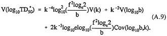
Rather than discard the 69 data sets for which mle's could not be obtained, we chose to fit a Weibull model to each of these data sets using a fixed value of the shape parameter k. In this regard, we first separated the 69 data sets into two subgroups based on their overall shape. A value of k = 1.7 was used for the 42 data sets that demonstrated clear upward curvature, this being the median value of k observed among the 68 of the 122 data sets for which k > 1. Similarly, a value of k = 0.55 was used for the 27 data sets exhibiting downward curvature, this being the median value of the 54 of the 122 data sets for which k < 1. The variance of log10TD*/50 was then estimated using (A.9), with k treated as an estimated rather than a known parameter. Allowance for some degree of uncertainty in the value of k is desirable in order not to severely underestimate the variance of log10TD*/50 (cf. annex B).
The 26 data sets in which only a control and single dose group were available were not used here since no information on the shape of the dose-response curve is available.
Annex B. Shrinkage Estimators of the Distribution of Carcinogenic Potency
The distribution of TD50 values for a series of chemical carcinogens provides useful information on the variation in carcinogenic potency. Because each estimate ![]() of the true TD50 for a specific chemical is subject to estimation error, the distribution of estimated potency values
of the true TD50 for a specific chemical is subject to estimation error, the distribution of estimated potency values ![]() will exhibit greater dispersion than the distribution of true potency values (TD50s). This overdispersion may be eliminated using empirical Bayes shrinkage estimators (Louis, 1984).
will exhibit greater dispersion than the distribution of true potency values (TD50s). This overdispersion may be eliminated using empirical Bayes shrinkage estimators (Louis, 1984).
Let Y = log10TD50 and suppose that E(Y) = µ = log10TD50, with V(Y) = s2. Let Y1,…, Yn denote the logarithms of the estimated TD50 values for a series of n chemical carcinogens. We suppose that Yi is normally distributed with mean µi and variance si2. We further suppose that µi are normally distributed with mean µ and variance t2 where t2 reflects the variance among the µi. Our objective is to estimate µ and t2, and hence describe the lognormal distribution of unknown TD50 values.
Noting that
an estimator of t2 is
where ![]() and
and ![]() is the estimator of V(log10TD50) based on (A.9).
is the estimator of V(log10TD50) based on (A.9).
The shrinkage estimator of µi is given by
where ![]() represents an estimator of the intrastudy correlation,
represents an estimator of the intrastudy correlation, ![]() is an estimator of the overall mean of the log potency distribution, and
is an estimator of the overall mean of the log potency distribution, and
is designed to protect against overadjustment for overdispersion. In general ![]() < 1, so that the estimators
< 1, so that the estimators ![]() of the µi are obtained by
of the µi are obtained by


