
the sample size n are shown in Table 1. (Note that the values of h1 and h2 are implicit functions of n.) These results are based on a one-stage model (k = 1) with a spontaneous response rate p0 = 0.10, and a nominal significance level of γ = 0.05 with r = 10 in the case n = 50. The value of σ2 = V(logeMTD) = 8.196 is based on the variance of the MTD of the 191 experiments considered previously by Krewski et al. (1990b). Using common logarithms, V(log10MTD) = 1.546.
The dependency of the correlations between log10TD50 and logeMTD on the Weilbull shape parameter k is illustrated in Table 2 for a sample size of n = 50. These results, including the limiting cases as k → 0 or ∞, are also based on (D.13). Note that the correlation remains high regardless of the value of k.
Annex E: Correlation Between TD50s For Rats and Mice
In this annex, we derive analytical expressions for the correlation between TD50 values for rats and mice. Letting Yrats and Ymice denote the logarithms (basee) of the estimated TD50s for rats and mice, we seek an expression for ρ = Corr(Yrats, Ymice). Following Bernstein et al. (1985) we assume initially that the MTD for rats is directly proportional to that for mice, with
Using the notation of annex D, we will denote the logarithms of the MTDs for rats and mice by Xrats and Xmice, so that
Note that (E.2) implies that V(Xrats) = V(Xmice) = σ2
As in annex D, we assume that the TD50s for rats and mice are uniformly distributed about their respective MTDs. From (D.10), we may then write
where h1 and h2 are the same for rats and mice since g1 and g2 defined in (D.4) and (D.5) respectively are the same for rats and mice. Assuming that Yrats and Ymice are conditionally independent, given MTDmice (and hence MTDrats from (D.1)), we have
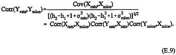
Hence
where ρ = Corr(Yrats, Xrats) is given in (D.13) of annex D. Based on the n = 127 compounds from the CPDB considered in section 6.1, we find σ2rats = 10.065 ≈ σ2mice = 8.873. For σ2 = 10, we have ρ = 0.943.
The assumption (D.1) of strict proportionality between MTDrats and MTDmice can be relaxed. Let V(Xrats) = σ2rats and V(Xmice) = σ2mice . As in (D.3), we have
and
Assuming Yrats and Ymice are conditionally independent, given Xrats and Xmice, we have
and hence
For the n = 127 compounds considered in section 6.1, we estimate Cov (Xrats, Xmice) = 7.638, and ρ = 0.763


