
Appendix C
Source Identification and Apportionment Models
SPECIATED ROLLBACK MODELS
The speciated rollback model is a simple, spatially averaged mathematical model that disaggregates the major airborne particle components into chemically distinct groups that are contributed by different types of sources (Trijonis et al., 1975, 1988).
A linear rollback model is based on the assumption that ambient concentrations C above background are directly proportional to total emissions E in the region of interest. Stated as a formula, C-Cb = kE, where Cb is the background concentration due to emissions other than E (i.e., to emissions outside the region of interest; natural sources, even inside the region, are usually included in this background term). The constant of proportionality, k, is determined over a historical time period when both concentrations, C and Cb, and regional emissions, E, are known. With that information, new concentration estimates can be derived for proposed changes in emission levels. For an inert pollutant, the only assumption required for the model to be exactly correct at all points in the region is that the relative spatial distribution of emissions remains fixed despite the changes in emissions. 1 That assumption be-
comes less restrictive when the model is applied to larger, three-dimensional, and spatially averaged concentrations rather than to concentrations at individual points in a geographic region. Thus, the model is especially useful for spatially averaged problems, such as regional haze.
A speciated rollback model for airborne particles is an aggregation of several separate rollback models for each individual chemical component of the atmospheric particle complex. In almost all cases, the anthropogenic materials in the dry particle mass almost entirely consist of five components: sulfates, organics, elemental carbon, nitrates, and crustal material (e.g., soil dust and road dust). Organics can be further subdivided into primary organic and secondary organic particles. In the simplest case, it is assumed that linear rollback models can relate each primary particle component (elemental carbon, crustal material, and primary organics) to its regionwide emission level and each secondary aerosol component (sulfates, nitrates, and secondary organics) to the emission level of its controlling gas phase precursor (e.g., SO2, NOx, NH3, and VOC).
In considering the ambient nature of airborne particles (not only the measured dry fine-particle mass), particle-bound water is an additional important component. Certain chemical constituents of anthropogenic particles—such as sulfates, nitrates, and some organics—have an affinity for water. The constituents acquire water vapor from the atmosphere and form a liquid phase at relative humidities well below the 100% level normally associated with condensation. If the concentration of hygroscopic particles (i.e., those that retain water) is reduced, there is a corresponding reduction in the particle-bound water. Accordingly, water retention is usually incorporated into the rollback models for the hygroscopic airborne particles (i.e., sulfate-bound water is assumed to change in proportion to sulfate concentrations at a particular relative humidity, nitrate-bound water in proportion to nitrate concentrations, etc.). For example, if one is considering a rollback model for visibility effects, the total light-extinction contribution from nonbackground sulfate particles plus sulfate-associated water is assumed to change in proportion to SOx emissions.
The speciated rollback model incorporates a very restrictive assumption in addition to the assumption about the spatial homogeneity of emission changes. The restrictive assumption is that there is only one controlling precursor for each secondary airborne particle component and that transformation and deposition processes are completely linear with
respect to the precursor (i.e., that transformation rates and deposition velocities are independent of pollutant concentrations).
Various complexities can be added to the speciated rollback model. First, rollback models can be disaggregated by particle-size fraction (e.g., coarse versus fine particles) as well as by chemical composition. Second, additional distinctions can be made between primary and secondary particles (e.g., separate rollback models can be formulated for primary versus secondary sulfate particles). Third, rather than using proportional relationships, nonlinearities in transformation processes can be approximately accounted for by assuming nonlinear functional relationships between emitted precursors and their atmospheric reaction products. Finally, the model can be disaggregated spatially by including separate transfer coefficients for different source areas or stack heights. The latter two modifications are ways of relaxing some of the restrictive assumptions of the rollback technique.
Four types of information are needed to implement a speciated rollback model:
-
Data on airborne particle concentrations disaggregated by components of the particles;
-
Knowledge or assumptions regarding the controlling precursor for each secondary airborne particle component;
-
Emission inventories for the important source categories of each airborne particle component and each gaseous precursor substance;
-
Knowledge or assumptions regarding background concentrations (due to sources other than those that are in the inventory) for each component of the airborne particles and each gaseous precursor substance.
One of the advantages of the rollback model is that this type of information is often obtained as a first step in any reasonable and practical control plan; therefore, rollback models often can be formulated and applied at an early stage in the source attribution process.
RECEPTOR-ORIENTED MODELS BASED ON CHEMICAL SIGNATURES
Receptor modeling is an active and developing field of research that has given rise to many different approaches and techniques. The follow-
ing discussion provides a taxonomical overview, identifying some recurrent themes and attempting to clarify the relationships among various models. We then focus on two models (i.e., chemical mass balance and regression analysis) that are used so often that a more detailed discussion of their formulation is warranted.
A variety of techniques extract information on the types of sources contributing to a given airborne particle sample on the basis of the particles' chemical composition. All the techniques are conceptually based on the same underlying model (Friedlander, 1977; Henry et al., 1984; Hopke, 1985; Gordon, 1988):
In Equation C-1, the subscripts i,j, and t index ambient aerosol characteristics, emissions sources, and sampling intervals, respectively. The terms ci, Sj, and fij are defined as follows:
ci is the ith characteristic of the airborne particles at the receptor site. That characteristic is typically the mass concentration (particle mass per unit air volume) of the particles or particle component. The characteristic also can be an air pollutant effect, such as the light-extinction coefficient (extinction cross-section per unit air volume) (Pitchford and Allison, 1984) or mutagenicity (revertants per unit air volume) (Lewis et al., 1988). For simplicity, our discussion will take the ci to be the mass concentration of the ith particle component.
Sj is the ambient mass concentration (effluent mass per unit air volume) of the total effluent contributed by the jth emissions source at the receptor site. This contribution often is referred to as the source strength. A source can be defined as a specific industrial facility, such as the Navajo Generating Station (NGS) at Page, Arizona (NPS, 1989; NRC, 1990), a generic category, such as soil dust (Friedlander, 1973), or a geographic area, such as the midwestern United States (Rahn and Lowenthal, 1985).
fij is the mass fraction (particle mass per effluent mass) as measured at the receptor site, of particle component i in the effluent of the jth source. The sequence f1j, f2j, fnj is referred to as the jth source's profile, or its chemical signature or fingerprint. For conserved chemicals, it may be possible to measure fij at the source (Core, 1989a). For
substances produced or destroyed in the atmosphere, measurements at the source may have limited value (NRC, 1990).
All the techniques have as their objective the estimation of the source contributions, fijSij.
A class of methods referred to as chemical mass balances (CMB) can be applied to the solution of Equation C-1 when the source characteristics fij are known. The simplest case involves a conserved substance i, which is emitted by a unique source j. Such a tracer can be endemic, such as lead in Los Angeles automobile exhaust during the early 1970s (Miller et al., 1972), or inoculated, such as deuterated methane (CD4) that was injected into the effluent of the Navajo Generating Station during the Winter Haze Intensive Tracer Experiment (WHITEX) (NPS, 1989; NRC, 1990). For the unique tracer, Equation C-1 simplifies to cit = fijtSjt, which can be solved directly for the source strength in terms of the measured ambient concentration of the tracer and the mass fraction of the tracer in the source's effluent: Sjt = Cit/fijt. The jth source's contribution to another conserved substance, one that may be emitted by multiple sources, then can be calculated from the mass ratio measured at the jth source:
In most cases sources are distinguished by overall chemical profiles rather than by unique individual substances. Such situations are typically modeled in terms of n conserved substances that are wholly accounted for by the emissions of m ≤ n sources. If the chemical profiles are linearly independent, then the system given by Equation C-1 (i = 1, n) can be solved for source strengths Sj (j = 1, m) in terms of the measured ambient concentrations ci and the source characteristics fij. To minimize the effects of measurement error, the number of substances is usually taken to exceed the number of sources (n > m), in which case an overdetermined solution is estimated by weighted least-squares fitting procedures (Watson et al., 1984). Useful information sometimes can be obtained even when there are more sources than substances (White and Macias, 1991). Given an estimate of source strengths, source contributions can be derived for any conserved substance, whether it is one of the n markers used in the solution or one with additional sources. If there are many more measured chemical
substances than sources, then the comparison of modeled concentrations with observed ambient concentrations of all chemical substances can provide a valuable internal check on model consistency (Friedlander, 1973; Kowalczyk et al., 1978).
The CMB model possesses some attractive properties as a tool for apportioning conserved characteristics of the ambient airborne particles. Unlike the statistical approaches discussed below (e.g., factor analysis), the CMB model can be applied to individual ambient samples. More critically, it is an easily understood and easily scrutinized model that is straightforwardly derived from physical principles, and it contains no unmeasured quantities. The CMB's deterministic character carries a cost, however; it requires comprehensive prior information on the identities and chemical characteristics of all important sources that contribute to the ambient aerosol.
When multiple ambient samples are available, a class of methods referred to as factor analysis offers empirical insights into the identities and characteristics of major sources. The basic idea behind factor analysis is that the ambient concentrations of various conserved chemical substances should correlate with each other if they have a common source. That idea can be seen in the simplest case, where j is the only source of substances i and i', and the source characteristics fijt = fij and fi'jt = fi'j are stable from one sample to the next. According to Equation C-1, the only source of variability in the ambient concentrations cit, = fijSjt and ci' = fi'jSjt is then the common source strength Sjt. The two concentrations should therefore correlate, both being high when source j is present and both being low when source j is absent; moreover, their standard deviations should be proportional to the substances' abundance at the source. Inverting that logic, one can hypothesize that substances that are highly correlated in ambient air have a common source, and one can infer the chemical signature of the source from ambient measurements alone.
Factor analysis provides a framework for partially extending the simple reasoning outlined above to situations with multiple sources. A sequence of p ambient measurements, each characterizing n substances, can be represented as a cloud of p points in n-dimensional space ("Q-mode analysis") or n points in p-dimensional space ("R-mode analysis") (Hwang et al., 1984). In either representation all points should, according to Equation C-1, lie within model and measurement error of the m-
dimensional hyperplane determined by the chemical profiles of the m distinct emissions sources. The algebra of factor analysis allows the dimensionality and orientation of this hyperplane to be estimated from the data. The source profiles themselves can be recovered in the special case where each substance has a unique source (via "VARIMAX rotation") or when the profiles are approximately known already (via "target transformation") (Hopke, 1985). Factor analysis thus serves to validate and refine the source information used in the CMB model. The set of source profiles cannot be recovered uniquely without some such prior knowledge, because the set constitutes only one of an infinite number of possible coordinate systems (Henry, 1987).
In the context of visibility studies, the models of CMB and factor analysis are critically limited by their restriction to airborne particle characteristics that are conserved during transport from source to receptor. As discussed in Chapter 4 of this report, the extinction cross-section of the ambient aerosol is contributed largely by secondary particulate matter, which is not directly emitted by any source, and is inflated by liquid water whose abundance is determined by ambient relative humidity conditions. The optical characteristics of source emissions are thus a function of atmospheric transport and transformation, and are highly variable relative to the tracer substances used in CMB and factor analysis. The optically relevant portion of a source's profile at the receptor site consequently cannot be determined by direct measurements of its emissions but must be estimated by source-oriented modeling or by regression analysis of ambient data.
Linear regression analysis is a well-established (Seber, 1977; Draper and Smith, 1981) and well-studied (Belsley et al., 1980; Fuller, 1987) class of procedures for estimating unknown coefficients in linear relationships from multiple observations of the dependent and independent variables. Equation C-1, adapted to account for the sulfate concentration, adapted to, for example, is a linear relationship in which the source-specific ratios of sulfate to effluent are unknown parameters. Given measured ambient sulfate concentrations cit, and ambient effluent concentrations Sjt derived from CMB analyses of conserved substances, regression analysis can generate estimates of the average sulfate-to-effluent ratios fij at the receptor. The regression estimates are determined by optimizing the agreement between measured and modeled sulfate values.
All the foregoing analyses require the existence of chemical signatures
for at least some of the sources of interest in a given application. To be broadly useful, such signatures must be distinctive, stable, and measurable. Because they minimize collinearity problems in the solution of the system described by Equation C-1, the most helpful signatures involve substances predominantly attributable to a single major source or source category. Table 5-2 lists examples of substances that have been used as endemic markers and the sources to which they are usually attributed. Endemic tags also have been identified for some airsheds that are rich in a distinctive source type (Rahn, 1981; Miller et al., 1990). Unique signatures can be created by inoculating targeted sources with substances that are otherwise scarce in the atmosphere (e.g., unusual perfluorocarbons, deuterated methane, or sulfur hexafluoride). Such artificial tags have been applied to specific sources (Shum et al., 1975; Georgi et al., 1987; NPS, 1989) and to airsheds (Reible et al., 1982; Haagenson et al., 1987). Artificial tracers often are used to elucidate airflow patterns. In such studies, the tracer is typically released in discrete puffs. In contrast, tracers used to support receptor modeling should be released over a sustained period to avoid ambient samples that contain an unknown proportion of tagged and untagged effluent. To study particle fluxes, it is necessary that (1) the ratio of tracer injected into the stack to stack gas-particle loading is constant, and (2) the dispersive and depositional characteristics of the tracer and primary particles emitted from the stack are similar.
The distinctiveness of an endemic source signature depends in general on its context. Several of the tracer-substances' source attributions in Table 5-2, for example, must be considered unreliable in the southwestern United States, where copper smelters are important sources of vanadium, arsenic, sellenium, and lead (Small et al., 1981). In actual applications, it can be difficult to verify the attribution of a signature to a specific source. At the large distances over which sources can contribute to regional haze, there may be many sources for any endemic tracer. A useful multi-substance signature based on characteristic substance ratios rather than characteristic substances per se, must preserve its distinctiveness over all combinations of all potential sources of any of the signature's constituents.
Fluctuations in source signatures can produce significant uncertainty in source apportionment. There is some variability, often undocumented, in the composition of emissions from any individual source. The SO 2-to-NOx ratio in the Navajo Generating Station's emissions varies by
about 20% (Richards et al., 1981), for example, and the sulfur-to-selenium ratios in two samples taken during WHITEX differed by a similar amount (NPS, 1989). Additional variability is introduced by the diversity in the chemical composition of emissions from the individual sources that make up a given source category, especially at the large distances relevant to regional haze. The selenium-to-aluminum ratios in fine-particle emissions from coal-fired power plants can vary by 70% (Sheffield and Gordon, 1986), for example, even for facilities located in the same geographic region and using similar particle control technology. Figure 5-1 shows copper smelters within the same geographic region to have widely varied chemical signatures. Even suspended soil dust varies significantly in composition from site to site (Cahill et al., 1981).
No chemical signature is of value unless it can be identified at ambient concentrations. In many national parks and wilderness areas, this requirement places heavy demands on measurement technology. For example, Table 5-1 shows that most of the tracers identified in Table 5-2, including vanadium, manganese, nickel, arsenic, selenium, bromine, and lead, were not quantified routinely by the trace-element monitoring network operated by the National Park Service between 1979 and 1986. The main problem is that a source's impact on visibility through the atmospheric formation of secondary particle components does not lessen with distance in proportion to the dilution of its primary emissions. Moreover, the detectability of chemical signatures does not necessarily improve with the progress of technology, because analytical advances complete with improved emissions controls. As one example, the decrease in automotive lead emissions since the mid-1970s has clearly outpaced increases in analytical sensitivity, making it difficult to use lead as a tracer for automotive aerosol emissions.
Recent use of CMB calculations and regression analysis as part of the visibility impairment study contained in the National Park Service's WHITEX report (NPS, 1989) has focused particular attention on those two source apportionment methods. For this reason, an extended discussion of both models follows.
CMB Models
The CMB model was first proposed by Winchester and Nifong
(1971), Hidy and Friedlander (1972), Kneip et al. (1972), and Friedlander (1973). It has been applied widely to apportionment of sources of primary particulate emissions on local and regional scales, to groundwater problems, and to apportionment of sources of VOCs and air toxics and of sources contributing to light extinction (Cooper and Watson, 1980; Hopke and Dattner, 1982; Hopke, 1985; Pace, 1986; Gordon, 1980, 1988; Watson et al., 1989). The CMB model has been used widely in the regulatory community (EPA, 1987c), and many validation studies have been completed with the model (Stevens and Pace, 1984).
The current state of the art limits the model's regulatory application to particulate matter that is directly emitted to the atmosphere. The ability of the CMB model to apportion airborne particle concentration or light extinction to sources is limited to categories of sources with dissimilar source profiles, because of the assumptions inherent in the model and because of its inability to resolve sources of secondary particles.
The first-order principles of the CMB model have been described (Watson et al., 1991), and assumptions implicit in its application have been documented in the literature (Watson et al., 1991). The sensitivity of the model to deviations from modeling assumptions has been examined in two studies, both of which were designed to determine if the CMB model could be used in regulatory settings (Stevens and Pace, 1984; Javitz et al., 1988a,b).
CMB source apportionment was first used as a basis for regulatory action by the state of Oregon, when in 1977, it sponsored the Portland Aerosol Characterization Study (PACS). PACS was the first large-scale, successful receptor modeling study specifically designed to support State Implementation Plan revisions to attain EPA's Total Suspended Particulate NAAQS (National Ambient Air Quality Standard). The study spawned much of the receptor modeling technology that is in use today (Watson, 1979). The source apportionment results developed during PACS were applied by the staff of the Oregon Department of Environmental Quality in the first joint applications of receptor and dispersion modeling (Hanrahan, 1981; Core et al., 1982).
Concurrent with the revision of the NAAQS for particulate matter, EPA released several guidance documents to state regulatory agencies that supported the use of the CMB model as a technical basis for PM10 control strategies (Pace and Watson, 1987; EPA, 1987c). (PM10 refers
to particles less than 10 µm in diameter.) EPA has continued to support state air regulatory agencies' application of the CMB model by continued development of software (Watson et al., 1991). Source profile information also is being gathered (Core et al., 1984; Shareef et al., 1988; Core, 1989a; Houck et al., 1989).
Theory of the CMB Model
Watson et al. (1990a,b) have described the theoretical basis of the CMB model in several publications.
The CMB model consists of a least-squares estimate of the solution to a set of linear equations that expresses each concentration of a chemical species at a receptor air-monitoring station as a linear sum of the products of source-profile species at the receptor site multiplied by source contributions. The source profile (i.e., the fractional amount of each chemical species in the emissions from each source type) and the ambient concentrations of each species measured at the receptor site with appropriate uncertainty estimates serve as input data to the model. The output consists of the ambient airborne particle mass increment and the amount of each chemical substance contributed by each source type. The model calculates values for the contributions from each source and the uncertainties associated with those source contributions. Input data on uncertainties are used both to weight the importance of input data on chemical species concentrations when computing the solution and to calculate the uncertainties associated with the source contributions.
Derivation and Solutions
The concentration of a conserved pollutant measured at a receptor air-monitoring site during a sampling period of length T due to a source j with a constant emission rate Ej is
where Dj is a dispersion factor depending on wind velocity u, atmospheric stability, and location of source j with respect to a receptor (x).
All these factors vary over time, so the dispersion factor D must be an integral over a specified time period. Various analytical expressions for D have been proposed based on solutions to equations that describe atmospheric transport, but none have completely captured the complex and turbulent nature of atmospheric dispersion. A major advantage of the CMB model is that an exact knowledge of D is not required. Instead the CMB model replaces Equation C-3 above with an equation of the form of Equation C-1, which was described earlier.
If the number of source types that contribute to the airborne particle mass is less than or equal to the number of aerosol chemical features measured, then Equation C-1 can be solved for the unknown source contributions, the Sj's by a variety of methods. These include tracer, linear programming, ordinary least-squares solutions, ridge regression, weighted least-squares solutions, and effective variance least-squares solutions (Britt and Luecke, 1973; Henry, 1982). An estimate of the uncertainty associated with the source contributions is an integral part of several of those solution methods.
The CMB software in current use by EPA applies the effective variance solution because it makes use of all available chemical measurements, it estimates the uncertainties of the source contribution estimates, and it yields the most reasonable solutions because it preferentially weights those chemical species with the higher precision in both source and receptor measurement. The effective variance solution is derived by minimizing the weighted sums of the squares of the differences between the measured and calculated values of ci and fij.
CMB Model Assumptions
Assumptions implicit in the version of the CMB model recommended by EPA include
-
The composition of the source emissions is not changed by transformation or deposition as the plume is dispersed downwind to the receptor, and the composition is constant over the time period of ambient and source sampling.
-
Chemical species do not react with each other—i.e., conversion of gases to particles and reactions between particles do not occur for the
-
species used for fitting a solution to the CMB equations. The chemical species are assumed to be linearly additive.
-
All sources with a potential for large contributions to pollutant concentrations at the receptor site have been identified, and their emissions have been characterized.
-
The relative chemical composition profiles that describe the emissions sources are linearly independent of each other.
-
The number of sources or source groups is less than or equal to the number of chemical species measured.
-
Measurement errors are not seriously correlated from one constituent to another and are not seriously biased (the calculation proceeds as though all correlations and biases vanish).
Assumptions 1 through 6 are fairly restrictive and will probably never be fulfilled totally. Fortunately, model validation studies using synthetic data sets have shown that deviations from the assumptions often can be tolerated by the model (within practical applications), although as the deviations increase, the uncertainties in the source contribution estimates also increase.
CMB Model Validation Studies
Validation studies (Stevens and Pace, 1984) have shown that the CMB model typically can resolve the separate contributions of five or six major emission sources to the ambient primary airborne particle mass. In simulations of a local airshed containing seven major sources—airborne soil dust, a coal-fired power plant, sea salt, a steel mill, a lead smelter, a municipal incinerator, and background aerosol—the CMB model was able to allocate the contribution of the coal-fired power plant to within an average relative uncertainty of ±50% and contributions of the oil-fired power plant to within an average of ±20%, even though the standard error of each source profile's daily fluctuation was 25% and the standard error of the airborne particle measurements was 10% (Javitz et al., 1988a). The studies focused on urban settings and excluded secondary sulfate contributions from the sources.
The studies indicate that, as the composition of the source emissions varies (Assumption 1), errors in the estimated source contributions also
vary in direct proportion to the magnitude of the bias. If the errors are random, the magnitude of the estimated error of the source contributions decreases as the difference between the number of species and sources increases. For that reason, use of the maximal possible number of fitting species in the model is encouraged.
Few studies have been performed on the basis of Assumption 2 (linear summation of species), but because errors introduced by the conversion of gases to particles and the reactions among particles are not necessarily linear, the model's ability to apportion secondary particles (taken as the quantity of ammonium, nitrate, sulfate, or organics that remains unexplained following apportionment of primary emissions) correctly among primary sources might be suspect. As chemical-reaction mechanisms and, in particular, the distribution of organic-reaction products become better understood, it might be possible to produce ''fractionated'' source profiles that can be used to apportion reactive species approximately among sources.
Regarding Assumption 3 (inclusion of correct profiles for all sources), model sensitivity studies have shown that (1) underestimation of the number of sources will have little effect on the calculated source contributions if prominent species contributed by unidentified sources are excluded from the calculation procedure; (2) if the number of sources is overestimated the contributions of those that are included will be underestimated because of the common properties of the emissions contributed by both included and excluded sources; (3) if major source types present in the airshed are excluded from the analysis, the calculated-to-measured ratio of the fitting species and other fitting criteria will prove unsatisfactory; and (4) if the number of sources is overestimated, the standard errors of the source contributions increase and the sources that are not present in the airshed are estimated to have smaller contributions than the standard errors of those estimates.
The linear independence requirement (Assumption 4) has been directly addressed in EPA's CMB software with inclusion of Henry's singular value decomposition analysis (Henry, 1982). When a model solution is reached that consolidates similarity clusters (groups of sources that cannot be resolved by the model), then the likelihood of significant errors due to collinearity is greatly reduced.
With regard to Assumption 5, the true number of individual sources contributing to receptor substances is usually much larger than the number of chemical species that can be measured. It is therefore common
practice to group sources that have similar chemical composition into composite source types. For example, wind-entrained soil dust, emissions from a rock crusher, paved-road dust, and agricultural-tilling dust often are grouped together into a "geologic" source type represented by a source profile that has the chemical composition of soil dust.
There are no results from validation studies currently available to judge the effect of deviations from Assumption 6 (randomness, normality, and uncorrelated nature of measurement uncertainties), but simulations (sensitivity studies) as well as theoretical development, support the focuses and relative emphases implied by the wording of that assumption.
Apportionment of Light Extinction
Since the CMB model only apportions airborne particle mass concentrations among source types, further calculations must be completed to use those source contribution estimates to apportion contributions to light extinction among source types. If the particle mass contribution at a receptor site is known from CMB calculations and the chemical composition of the particles is known, then the concentration of each chemical substances (typically primary SO42- and NO3-, organics, light-absorbing carbon, and fine-particle soils) contributed by the source can be calculated. Because the physical and chemical characteristics of the substance vary as a function of the environmental conditions (especially humidity), particle size, and particle shape, additional knowledge of the light-extinction efficiency (extinction-to-mass ratio coefficient in units of meters squared per gram) of each particle type (under assumed particle and atmospheric conditions) must be attained to calculate the contribution to the extinction coefficient associated with primary emissions from each source. Those extinction efficiency values are typically derived from the literature. Care must be taken to ensure that the extinction efficiency values represent the actual particle size, morphology, and humidity conditions that exist in the atmosphere under study.
Regression Analysis
Regression analysis generates empirical relationships of the form
between ambient concentration c and source strengths Sj, the terms being as defined following Equation C-1. Equation C-4 has no t subscript on the factors f; conventional regression analysis addresses only the average relationship of ci to the Sj, not the variations in this relationship from observation to observation. The subscript i on the mass or effect concentration ci usually can be dropped with no loss of clarity. In the terminology of regression analysis, c is the response, or dependent, variable; the Sj are the regressor, or independent, variables; and the fj are the regression coefficients.
In practice, the regressors are often taken to be variables that are proportional to source strengths, rather than the source strengths Sj themselves. The corresponding proportionality constants are then incorporated into the empirical regression coefficients. For example, tracer substances attributed to unique source types are commonly used directly as regressors, in which case the reciprocal of the tracer concentration in the emissions becomes an implicit factor of the regression coefficient. Apportionments based on such regressions do not depend on that possibly unknown factor, because it cancels out in the calculation of absolute contributions when the coefficient is multiplied by tracer concentration instead of source strength.
Background
Multiple regression has been widely used to apportion total particle mass among different types of emission sources. The most common approach has been to use tracer concentrations directly as regressor variables (Kleinman et al., 1980; Cass and McRae, 1983; Currie et al., 1984; Dzubay et al., 1984; Lewis et al., 1986; Valaoras et al., 1988). Lewis et al., (1986) and Dzubay et al. (1988) pre-treated their tracer data with mass balance techniques to remove nonautomotive contributions to lead and soil-derived contributions to other trace elements. Morandi et al. (1987) similarly employed preliminary regressions of multiple source tracers on unique source tracers to refine their regressors. Hopke et al. (1980), Thurston and Spengler (1985), and Pratsinis et al. (1988) in-
ferred source types through factor analysis of elemental data and used the factor levels as source strengths in subsequent regression analyses.
Multiple regression analysis also has been tried as a method for apportionment of ambient concentrations of particulate sulfur among contributing sources. Some approaches, like those for total mass reviewed above, rely on chemical information. Regressors can be source strengths derived through mass-balance techniques (Rahn and Lowenthal, 1985) or raw tracer concentrations (Dzubay et al., 1988). Other approaches exploit a superior knowledge of temporal and spatial patterns in sulfur emissions. Regressors can be emission rates that fluctuate daily (White et al., 1978) or monthly (Sisler and Maim, 1990) or binary indicators that tell whether a source is operating (= 1) or out of service (= 0) (Murray et al., 1990). Alternatively, regressors can be the prior residence times of sampled air over specific geographical regions, estimated by counting end points of calculated back-trajectories (lyer et al., 1987; Gebhart and Maim, 1990).
Aerosol chemical substances that have been apportioned among contributing sources by multiple regression include, in addition to sulfates, elemental and organic carbon (Daisey and Kneip, 1981; Shah et al., 1985; Lewis et al., 1988; Pratsinis et al., 1988) and total (gas plus particle phase) sulfur and nitrogen (White and Roberts, 1977; Malm et al., 1990). Regressions of all measured elements on a fixed set of marker elements have been used to complete the chemical profiles of sources for which only unique tracers were known (Currie et al., 1984; Lewis et al., 1986; Rheingrover and Gordon, 1988). Some regression analyses have taken light extinction (Khalil et al., 1983; Pitchford and Allison, 1984) or mutagenicity (Lewis et al., 1988) as the response variable, directly apportioning effects rather than the gravimetrically or chemically determined airborne particle mass. (Regression analysis is used more often to relate light extinction to the optically important airborne particle components, rather than to source tracers; that application was discussed in Chapter 4.)
Currie et al. (1984) tested the apportionment of primary particles among sources by multiple regression in a methods intercomparison study based on simulated data. Regression analyses generated independent estimates of the chemical composition of contributing sources that were reasonably consistent with the true chemical composition of those sources and provided estimates of source contributions to ambient particle mass concentrations comparable to those of CMB and other receptor-
oriented methods. Among the sources accurately characterized was an "unknown source," the existence of which had not been disclosed to the participants in the methods comparison study. The simulated data did not incorporate certain aspects of real atmospheric problems, most notably the variability of source effluent chemical composition from one observation to the next.
In the real atmosphere, regression-derived apportionments of predominantly primary airborne particle fractions have survived various cross-checks against emissions data. Cass and McRae (1983) found that the empirically estimated tracer contents of highway, oil-ash, and crustal source contributions were consistent with careful prior estimates based on local emissions source tests. Kleinmann et al. (1980) were able to relate results for motor vehicle and oil combustion fractions over several years to annual variations in the lead and vanadium contents of gasoline and fuel oil. Lewis et al. (1986) related differences in the empirically estimated lead contents of motor vehicle exhaust particles in different studies to differences in the prevailing lead content of gasoline.
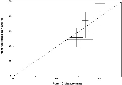
Perhaps the most convincing validation yet of the use of regression analysis as a source apportionment tool was produced by Lewis et al. (1988) in their work on mutagenicity. Those authors apportioned total carbon between wood smoke and motor vehicle exhaust, by regressing carbon on nonsoil potassium and lead. They then had several samples analyzed for 14C content, which is a direct indicator of the fraction of the total carbon that is due to contemporary (wood smoke) rather than fossil-fuel (motor vehicle exhaust) sources. Figure C-1 shows that the independent, nonstatistical 14C measurements nicely confirm the source apportionment results obtained by regression analysis. The closeness of the correlation (r = 0.88) is the more impressive when we note that the fluctuations in absolute carbon concentrations, which would contribute common variability to both determinations, have been factored out in this presentation.
The accumulation of published successes does not wholly dispose of what has been called "the file drawer problem" (Rosenthal, 1987). This is the problem that uncounted file drawers might be filled with regression analyses that were never published because they failed available cross-checks. Regression analysis is of greatest interest in precisely those applications for which emissions data do not exist, and alternative approaches are infeasible. It is of little value to know that regression analysis sometimes gives valid results, if there is no way to identify
whether a particular analysis, which cannot be checked, is in fact producing the correct answer. Regression must be demonstrated to work nearly all the time in specified contexts, and that can be established only through formal trials that report all results, the failures and the successes.
The apportionment of predominantly secondary aerosol fractions by regression has yet to be rigorously tested. Apportionments of total mass have not addressed regression's performance on secondary material, because secondary substances such as sulfates and nitrates usually have been included as regressors in their own right (Kleinman et al., 1980; Cass and McRae, 1983; Dzubay et al., 1984; Lewis et al., 1986; Morandi et al., 1987; Dzubay et al., 1988). Sulfates and nitrates have thus been treated as explicit categories in the mass apportionments, with only the remaining, undifferentiated, predominantly primary material apportioned among sources types. Lewis et al.'s (1988) validation of their source apportionment study did not relate to secondary substances, because their data were from the winter, when photochemical conversion would have been minimal. No attempt has been made yet to replicate Currie et al.'s (1984) evaluation study with atmospheric conversion processes included in the simulated data base. By the nature of the secondary particle problem, cross-checks against source measurements are not helpful.
The support available for regression-derived apportionments of secondary particles is largely based on demonstrations of the internal consistency of the results obtained. Lowenthal and Rahn, 1988, for example, showed that the regression model of Rahn and Lowenthal (1985) yielded reproducible coefficients when fit to data from different years. Murray et al. (1990) noted that their regression coefficients yielded estimated source impacts that were least at their upwind monitor and greatest at the closer of two downwind monitors.
Statistical Assumptions and Consequences of Violation
Regression analysis determines coefficients fj for the regression model described by Equation C-4 that optimize its fit to the data for ambient concentrations ct and source strengths Sjt. Model fit can be character-
ized in various ways. Nearly all source apportionment analyses have employed ordinary least-squares (OLS) regression, which minimizes the mean squared difference between modeled and observed values of the response variable. The OLS approach models ambient concentrations as the sum of deterministic and random contributions:
the deterministic component being the linear relationship of Equation C-4. The scatter in the observations is represented as a random error, ![]() in this relationship.
in this relationship.
The scatter in Equation C-5 arises most fundamentally from the fact that the true coefficients fjt generally fluctuate from observation to observation, as indicated in the original Equation C-1. Such fluctuations can be pronounced particularly in applications to visibility, where fjt typically represents a ratio of secondary airborne particles to primary tracer. Such a ratio varies widely with the age of the emissions, atmospheric oxidant concentrations, atmospheric liquid water content, and other atmospheric factors. The approximation of the fluctuating relationship by a constant one can thus introduce significant errors in individual observations if the estimated value of fj is later used to try to explain the relationship between individual observations of ct and Sjt.
Additional scatter is introduced when source-strength estimates Sjt are unavailable for some categories of emissions. The standard practice is to treat untagged emissions collectively as "background" and represent the background in the regression equation as a constant term f0, which represents the aggregate contribution of all untagged sources. In the geochemical community, the term "background" is usually reserved for contributions that are globally uniform or are predictable functions of latitude or altitude, for example. In regression analyses of air pollution, however, the background of untagged emissions typically varies just like any other component of the mix, and so is poorly predicted by any average value.
On the operational level, scatter arises from uncertainties in the determination of source tracer concentrations. Chemical concentrations are measured with only finite precision, and the precision can be rather poor because of the low primary pollutant concentrations measured in many
regional haze analyses. Random errors in estimated source tracer concentrations clearly translate into random errors in predicted ambient concentrations. An analogous problem is that the ratio of tracer species emissions to total emissions from a source may fluctuate, reflecting inhomogeneities in fuels and feedstocks. Those fluctuations are similar to measurement errors in their effects on estimated source contributions to ambient samples.
Finally, the underlying relationship (Equation C-1), might involve a stochastic component, and be inherently imprecise itself. For example, the ambient mass or effect concentration c and the source strengths Sj might be measured in different air volumes. The comparison of path-averaged optical measurements with point measurements of aerosol chemical composition furnishes a common illustration of such a mismatch, as noted in Chapter 4.
The error in a regression relationship's reproduction of individual observations is of minor interest in most applications to source apportionment. Apportionments instead focus on the coefficients fj which represent empirical estimates for the mean values m(fjt) of the unknown source characteristics fjt. Those estimates are multiplied by the observed mean source strengths Sj = m(Sjt) to derive the estimated mean source contributions fjSj = m(fjtSjt). (That multiplication is grounded in the assumption that any fluctuations in the source characteristics are uncorrelated with variations in the source strengths, an assumption that is implicit in the representation of the source-ambient relationship as linear.)
Because of the empirical scatter in the relationship of ambient concentrations to source strengths, one cannot hope to determine mean source characteristics exactly with a finite number of observations. It seems reasonable to expect the estimation procedure to be unbiased, however, yielding results that are neither systematically high nor systematically low. It also seems reasonable to expect the estimates to be consistent, approaching the correct values as the number of observations increases. An advantage of the OLS approach over other forms of regression analysis is that the conditions required to establish the desirable properties are simply stated and do not involve the often unknown magnitudes of the relationship's random elements. For the OLS estimate—and for most other estimates that are often used—to be unbiased and consistent, it is sufficient that the error ![]() in Equation C-5 be statistically independent of the source strengths Sj (Goldberger, 1964).
in Equation C-5 be statistically independent of the source strengths Sj (Goldberger, 1964).
The condition that ![]() be random, varying independently of the Si, is a familiar assumption in statistical analysis, one seemingly legitimized by repeated invocation. However, a closer consideration of the physical relationship of ambient concentrations to estimated source strengths reveals several potential sources of correlation between
be random, varying independently of the Si, is a familiar assumption in statistical analysis, one seemingly legitimized by repeated invocation. However, a closer consideration of the physical relationship of ambient concentrations to estimated source strengths reveals several potential sources of correlation between ![]() and one or more of the Sj.
and one or more of the Sj.
An absence of source-strength estimates for major contributors to the ambient mix is perhaps the most obvious source of probable bias in regression-derived apportionments. The potential magnitude of such bias can be illustrated by a simple calculation. Suppose that a particular source emits a tracer X from which its strength S1 in the ambient atmosphere can be determined accurately. For simplicity, suppose also that the pollutant of interest is emitted in constant proportion to X and conserved in the atmosphere. The source-ambient relationship then can be written as ct = cbt + fXS1t, where cbt is the fluctuating background contribution of untagged pollutant and fX = cXt/S1t is the constant ratio of tagged pollutant to source strength. The sole source of scatter in the regression model ct = f0 + f1S1t is then the variation cbt-m(cbt) in background concentration. The regression coefficient f1 is linear in c = cb + cX, and is therefore the sum fb + fx of the regression coefficients of cb and cX on S1. The bias in regression's attribution of pollutant to the tagged source is thus
The regression coefficient fb can be expressed in terms of more elementary statistics (e.g., Edwards, 1984) as
r and s being the usual correlation coefficient and standard deviations.
The quantities s(cb) and r(cb, S1) appearing in Equation C-7 are unknown, but can be roughly estimated by empirical rules of thumb. One such guide, for ambient concentrations of pollutants with moderate atmospheric lifetimes, is that the standard deviation and mean are generally of comparable size (e.g., Hammerle and Pierson, 1975; Tuncel et al., 1985). (That regularity is related to the common observation that
concentration distributions are approximately lognormal (Ott, 1990): the ratio s/m for a lognormal distribution is a relatively weak function of the geometric standard deviation sg (Aitchison and Brown, 1957), with X at sg = 2.3.) The substitution of m(cb)/m(S1) for s(c)/s(S1 ) in Equation C-7 greatly simplifies the formula for bias:
The ambient correlation of unrelated emissions can be seen in the observed correlations of distinct source tracers or calculated source strengths where these are available. Such ''spurious'' correlations are clearly source-and site-specific, but are commonly substantial: Hammerle and Pierson (1975) found that r = 0.79 between lead (motor vehicles) and vanadium (fuel oil and soil dust) in the Los Angeles basin, for example; Lewis and Macias (1980) found that r = 0.45 between lead and selenium (coal) in West Virginia. Correlations with untagged emissions can be inferred by extrapolating from those observations, or by considering the common influence of meteorology on all emissions. As an example of the latter, Samson (1978, 1980) found that r > 0.5 between the eastern United States sulfate concentrations and the reciprocals of upstream wind speeds. Similarly, Patterson et al. (1981) found that r = 0.4 in the East between regional-average reciprocal visual range and regional-average air-mass residence time.
Our simple calculation is completed by setting r(cb, S1) = 1/2 in Equation C-8, as an approximate value. The bottom line is then that regression analysis can attribute incorrectly half of the untagged emissions to the tagged source: 2/3 of the ambient total can be attributed to a source that actually contributes 1/3, for example. That amounts to a sizable bias, unless the tagged emissions dominate all other contributions, in which case sophisticated data analyses are probably unnecessary in the first place.
Poor source-strength estimates are another straightforward source of bias in regression-derived apportionments. Errors in the measurement of a chemical signature, or fluctuations in its relationship to source strength, clearly degrade its performance as a predictor of ambient pollutant concentrations. This random empirical decoupling is manifested as a systematic depression of the corresponding regression coefficient.
The effect of imprecision on regression coefficients is easily understood in the case where only one source is considered. Suppose that estimates S'1 of the source strength S1 are accurate on average, but contain a random error δ1. Consider the actual and ideal regressions c = f'0 + f'1S'1 and c = f0 + f1S1 of ambient concentration on estimated and true source strengths. The regression coefficient for S1 is f1 = cov(c, S1)/s2(S1), where cov(x, y) = (n-1)-1t![]() (x-m(x))(y-m(y)) is the covariance (Edwards, 1984). Simple algebra shows the regression coefficient for S'1 to be f'1 = cov(c, S1 + δ1)/s2(S1 + δ1) = [cov( c, S1) + cov(c, δ1)]/[s2(S1) + 2 cov(S1, (δ1) + s2(δ1)]. Since the error δ1 is random, we may assume its correlation, and hence covariance, with S1 and c to be negligible. The formula for the degraded coefficient then simplifies to f'1 = f1F1, where
(x-m(x))(y-m(y)) is the covariance (Edwards, 1984). Simple algebra shows the regression coefficient for S'1 to be f'1 = cov(c, S1 + δ1)/s2(S1 + δ1) = [cov( c, S1) + cov(c, δ1)]/[s2(S1) + 2 cov(S1, (δ1) + s2(δ1)]. Since the error δ1 is random, we may assume its correlation, and hence covariance, with S1 and c to be negligible. The formula for the degraded coefficient then simplifies to f'1 = f1F1, where
Equation C-9 shows that random errors in the estimation of a source strength depress the corresponding regression coefficient by a factor F < 1, sometimes called the reliability coefficient (Cochran, 1968), involving the ratio of error variance s2(δ) to true variance s2(S). When the mean tracer concentration is near the detection threshold, the analytical precision s(δanal) of the tracer measurement is by definition approximately half the mean. As noted earlier, the standard deviation [s2(S) + s2(δ)]1/2 of the measured tracer concentration is typically approximately equal to the mean. The reliability coefficient near the detection threshold is thus bounded above by 3/4 because of analytical error alone. Relative analytical error declines as concentrations increase, but other sources of imprecision need not. In particular, fluctuating signatures can yield imprecise estimates of source-strength at all concentrations. The imprecision of source-strength estimates is sometimes evident in the imperfect correlation of different tracers for the same source: a reliability coefficient of 3/4 corresponds to a correlation of r = 0.87.
The effect of imprecision is amplified in multiple regression analysis by the covariation of different sources' strengths. Consider, for example, the actual and ideal regression equations c = f'0 + f'1S' 1 + f'2S'2 and c = f0 + f1S1 + f2S2. Suppose the estimates S'1 and S'2 to be precise and approximate, respectively (F1![]() 1 and F2 < 1), and let r = r(S1, S2) be the correlation among the true values. More simple algebra
1 and F2 < 1), and let r = r(S1, S2) be the correlation among the true values. More simple algebra
then shows the degraded coefficient of S'2 (Cochran, 1968) to be given by
For F2 = 3/4 and r = 1/2, as assumed earlier, Equation C-10 yields f2 = 0.7f2: the regression coefficient for the poorly characterized source is low by about 30%. The estimated contribution f'm(S') = f'm(S) is low by the same amount. Of course, this estimate is an improvement over that obtained by ignoring the imperfect signature and treating the second source as an undifferentiated part of the background. We have already noted that regression analysis will underestimate the contributions of untagged sources by about 50% for the same assumed degree of covariance.
Just as regression analysis tends to attribute untagged emissions to tagged sources, it also tends to attribute poorly tagged emissions to well-tagged sources. The degraded regression coefficient corresponding to the well-characterized source in our two-source example (Cochran, 1968) is given by
Suppose the true contribution of the poorly characterized source to be twice that of the well-characterized source, so that f2m(S2) = 2f1m(S1). The estimated contribution of the well-characterized source for F2 = 3/4 and r = 1/2 is then f'1m(S1) = 1.3f1m(S1), or about 30% high. Once again, that is an improvement over the 100% overestimate obtained earlier, under the same conditions, by completely ignoring the imperfect signature.
Other potential types of bias in regression-derived source apportionments are less predictable in their effects. Prominent among the types are fluctuations in the true coefficients fjt that correlate with one or more source strengths. In regression analysis of secondary pollutants, fjt and Sjt may be correlated because of their dependence on common environmental influences. Physically, fjt and Sjt, in that case are measures of conversion and (reciprocal) dispersion, respectively. Their statistical
association depends on the empirical balance of competing influences. In dry air, for example, both conversion and dispersion of sulfur are promoted by strong insolation; this coupling would tend to generate negative correlations r(f, S) < 0. In other seasons and settings, sulfur conversion is promoted by fog and low stratus, which are associated with poor dispersion; this coupling would tend to generate positive correlations r(f, S) > 0. These examples are only two of many common influences that can be identified.
Spurious correlations can be detected sometimes by repeating the regression analysis while using a different response variable, one not expected to depend on the given source strengths. Newman and Benkovitz (1986), for example, used that technique to cast doubt on the physical relevance of a regression analysis presented by Oppenheimer et al. (1985). Oppenheimer et al. had shown that precipitation sulfate concentrations in the western United States were linearly related to SO2 emissions from nonferrous metal smelters; Newman and Benkovitz pointed out that precipitation concentrations of elements that were not present in smelter emissions exhibited a similar relationship to SO2.
Practical Guidelines
From the foregoing discussion, it is possible to identify some critical elements in measurement programs designed to support source apportionment studies that are based on regression analysis. The foremost objective of such a program must be to provide accurate estimates for the source strengths of all major contributors to the ambient mix. If a substantial fraction of the ambient total cannot be related to specific sources, then this undifferentiated background must be characterized directly.
Our discussion above shows that standard multiple regression analysis tends to overestimate the contributions of well-tagged sources to the ambient mix. Statistical procedures have been developed to compensate for imprecision in source-strength estimates (Fuller, 1987; White, 1989a,b), but it is clearly preferable to design measurement programs to provide the necessary precision in the first place. Posterior corrections have received little practical testing, and are sensitive to input statistics that themselves must be estimated. They cannot help, in any event, with
sources whose strengths are not even roughly estimated because chemical or other signatures are altogether unavailable.
Some sources that lack endemic tags can be inoculated with artificial tracers to provide ambient source strengths that are measurable and that complete the data base. However, no artificial tracer, no matter how accurately and sensitively it can be measured, can substitute for balance in the experimental design. Tags are needed for all significant sources, not just the specific targets of regulatory or other interest (NRC, 1990).
When endemic or artificial tags cannot be found for a substantial fraction of the ambient pollutant concentration, our analyses show the necessity of characterizing this undifferentiated background by direct measurement, rather than estimating it as a by-product of the regression analysis. Of course, only total concentrations can be measured; the background concentrations can be measured only at times and places in which tagged emissions are absent. Such measurements are relevant, however, only if the background concentrations under these conditions are similar to those in the presence of tagged emissions. Since meteorological factors tend to impose a common temporal pattern on all ambient concentrations, as noted earlier, it is generally risky to estimate the background concentrations in one period from a measurement in another period. Simultaneous measurements made at different locations are often easier to defend.
When the tagged emissions form an identifiable plume, measurements made outside the plume provide unambiguous background data (e.g., White, 1977; Richards et al., 1981; White et al., 1983). If the measurements made to either side of the plume show similar concentrations, these background concentrations can be assumed representative within the plume as well. That interpretation must be invoked with care, of course, because valleys and other terrain features may channel untagged emissions along with the plume under certain conditions. Alternatively, the background can be measured upwind of a tagged source (e.g., Murray et al., 1990; NRC, 1990). For distant sources, this is a less desirable determination, because it is far from the receptors and lacks the consistency check that measurements to either side of the plume provide. Neither lateral nor upwind measurements can be consistently relied upon in extended stagnation episodes, when tagged emissions may diffuse throughout an entire airshed.
A final design consideration is the potential for reducing the risk of spurious correlations in regression analyses involving secondary pollutants by modifying the regression model to incorporate deterministic estimates of the atmospheric conversion of primary pollutants to form secondary reaction products. In this strategy, our mechanistic understanding of atmospheric chemical reaction processes is used to express the fluctuating ratio of secondary product concentration to source strength as a function fjt = gj(aget, UVt, RHt ...; h1, h2,...) of known external variables and unknown internal parameters. Regression analysis, possibly nonlinear, is then required to estimate only the constant parameters, as in applications to primary pollutants. Latimer et al. (1990) took the initial steps in this direction, but they employed a model that this committee judged to be unrealistic (NRC, 1990).
PLUME BLIGHT MODELS
Models for the visual appearance of plumes incorporate a model for computing pollutant concentrations in the plume and schemes for calculating radiative transfer processes that describe the visual aspects of the resulting plume. The pollutant reaction and transport codes that can be embedded in such a model range from simple Gaussian plume models to much more detailed numerical models that incorporate a mechanistic description of atmospheric chemical processes.
Plume blight models that are recommended for use by EPA have been built around the premise that plume dimensions and transport can be accurately represented by Gaussian plume equations. Such models contain modules for estimating the height of plume rise above its release point, a mathematical description of the expected plume transport and spread, estimation of the observer-plume orientation, and expected modulation of light intensity caused by the plume against the background.
The concentration χ of trace components at height z and lateral distance y from the axis of a plume can be estimated by using the Gaussian plume model for a continuous emission source whose effluent travels with constant wind speed u at plume elevation H (including plume rise) with lateral and vertical dispersion coefficients σy and σz, respectively, and is expressed as
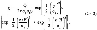
This equation is strictly for a conservative species, although the evaluation of chemically reactive species has been incorporated through temporal modification of Q.
The Gaussian plume model found within typical models for plume visual appearance can be replaced by a more advanced class of model known as a reactive plume model. Each of the models of this type cited below provide cross-wind resolution, at least in the horizontal. A grid system is defined within the air volume being modeled, and cross-wind diffusion proceeds according to Fick's law (flux proportional to the concentration gradient). An example of the strategy used for transport calculations is described in some detail by Stewart and Liu (1981).
The earliest of these models, by Eltgroth and Hobbs (1979), incorporates the conversion of SO2 to sulfate particles by homogeneous photo-chemistry and by first-order catalysis that might occur on soot particles. The model represents the particle size distribution in terms of three dynamic lognormal modes that evolve in response to homogeneous nucleation, coagulation, condensation, and gravitational settling. Light-scattering calculations are based on this computed particle size distribution. Other reactive plume models have been developed by Hov and Isaksen (1981), Seigneur (1982), Seigneur et al. (1982), Hudischewskyj et al. (1987), and Joos et al. (1987).
The most recent reactive plume and aerosol model by Seigneur and his co-workers (Hudischewskyj and Seigneur, 1989) represents the present state of the art. It is assembled from free-standing modules for transport, chemistry, and aerosol dynamics, each the product of considerable evaluation and testing in its own right. (An example of the scrutiny to which individual modules have been subjected is the intercomparison of aerosol dynamics modules by Seigneur et al. (1986).) The gas-phase chemistry module is based largely on an update of the carbon bond mechanism (CBM-III) introduced by Whitten et al. (1980). Phase equilibrium, including the partitioning of water, is based on the
model for an aerosol reacting system (MARS) introduced by Saxena et al. (1986). Aqueous-phase chemistry includes oxidation of SO2 by H2O2 and O2, the latter being catalyzed by MN2+ and Fe2+ (Saxena and Seigneur, 1987). The evolution of the particle size distribution, through homogeneous nucleation, coagulation, diffusion-limited condensation and evaporation, aqueous reaction, and sedimentation, is based on the sectional techniques introduced by Gelbard (1984).
MODELS FOR TRANSPORT ONLY AND FOR TRANSPORT WITH LINEAR CHEMISTRY
An analysis of wind flow during sampling periods is a necessary but insufficient test of source apportionment. There must be evidence of a reasonable probability of transport from the suspected source areas to the receptors during episodes of decreased visibility. Two options for assessment of the probability of transport are the application of models that: (1) assess only the transport of pollutants without regard to the chemical or physical processes affecting the pollutant, and (2) assess the transport but also include relatively simple linear chemical transformation processes.2 Analyses can be conducted through investigation of wind flow either to a receptor region or from a source area. The following section discusses transport analyses using (1) backward trajectories, (2) wind field analyses, and (3) transport models that incorporate linear chemistry.
Back Trajectory Analysis
Backward trajectory analyses are a fundamental meteorological tool used to assess the spatial domain of source areas that could have contrib-
uted to a volume of sampled air. Trajectories can be stratified by concentration or direction to ascertain the consistency of the relationship between air movement from a source area and the resulting pollutant concentrations at a receptor site. Back trajectory analysis provides an estimate of the mean path followed by air en route to a sampling location. It is understood, but seldom articulated, that the estimate represents only the path with the highest probability that transport occurred along that line. The actual transport path is more accurately represented by a two or three-dimensional probability density function.
Trajectory calculations conducted over large regions of the United States are made by interpolation of available wind observations (or, in some cases, wind analyses from hydrodynamic models) in time and space from observations made every 12 hours at sites 400–500 km apart. In some urban areas, there are denser networks of wind stations that allow trajectories to be constructed from hourly observations taken at locations that are tens of kilometers apart. The most widely used trajectory models employ a linear interpolation in time and a l/r2 spatial interpolation (where r is the distance from the trajectory to an observation point). A commonly used approach is the operational model of Heffter (1980), which employs available upper-air measurements assembled by the U.S. Air Force and the U.S. National Oceanic and Atmospheric Administration3 to calculate trajectories for either pre-defined or "mixed-layer" thicknesses.
A variety of techniques have been developed that make use of ensembles of trajectories to estimate the most probable source areas that contribute to regionally transported pollutants. Ashbaugh (1983) and Ashbaugh et al. (1985) used trajectories calculated by the Heffter (1980) trajectory technique to calculate the residence times of air parcels over 3-day trajectories for relatively high-sulfate versus low-sulfate concentrations. Such techniques have the advantage of indicating both the direction and speed of wind over the course of an air parcel's transit from source to receptor. They also serve the purpose of identifying qualitatively which air masses are consistently related with high or low pollut-
ant concentrations. That information might be valuable in determining whether regions of consistently pristine air exist ("clean air corridors" as defined in the Clean Air Act Amendments of 1990).
The uncertainties inherent in individual trajectories can be reduced when considering an ensemble of trajectories. If it can be assumed that the errors in each trajectory calculation are stochastic and that the estimated paths are not biased, then the results of ensemble trajectory analysis (ETA) can be expected to identify source areas that consistently influence observed concentrations. ETA uses simple stratification of trajectories by concentration or through weighting of estimates of the probabilities that transport to a particular receptor site will occur from all of the possible surrounding source areas.
The estimation of transport relationships for a given sampling time should include representation of the spatial variability. The probability of a reactive, depositing pollutant (such as SO2) arriving at two-dimensional point x in the horizontal plane of an airshed at time t, Ar(x, t), can be expressed (Cass, 1978) as
where T(x, t|x,', t'), the potential mass transfer function in two dimensions, is defined by relationships of the general type
where Q(x, t|x', t') is the transition probability density that an air parcel located at x' at time t' will arrive at receptor x at time t, R(t|t') is the probability that the pollutant of interest in that air parcel will not react to form another species from time t' to time t, D(x, t|x', t') is the probability that the pollutant will not be dry deposited between (x', t') and (x, t) and L(x, t|x', t') is the probability that the pollutant will not be wet deposited during transport from (x', t') to (x, t). The integration is conducted over time period τ. The reaction and deposition terms (e.g., the last three probability functions on the right side of Equation C-14) have been quantified by many authors and can be modified to account
for the interdependence of reaction, transport, and deposition processes and for the case of accumulating pollutants, like aerosol sulfate particles, that are formed by chemical reaction during transport in the atmosphere. Ignoring those terms allows the estimation of source-receptor relationships due to transport alone. Including those terms allows the estimation of source-receptor relationships incorporating linear transformation and removal.
The transition-probability density function, Q(x, t|x', t'), must be estimated with a transport model. For single or multiple-layer trajectory models, the axis of the computed trajectory can be assumed to represent the highest probability at any time that a particular upwind path is contributing to the trace substance composition at the monitor location. The spatial distribution of the transition-probability density function away from the axis of the trajectory can be adjusted to depend on meteorological conditions. As a first approximation, it was assumed by Samson (1980) that the ''puff'' of transition probability is normally distributed around each trajectory branch with a standard deviation that is increasing linearly in time upwind. Thus Q(x, t| x', t') is assumed to be expressed as
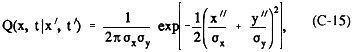
where x" = X-x'(t') and y" = Y-y'(t'); X and Y are the coordinates of the computational grid used to represent the airshed, and x'(t') and y'(t') are the coordinates of the centerline of the trajectory. It is assumed that σx and σy can be approximated by
with a dispersion speed, a, equal to a values believed to lie roughly between 1.8 and 5.4 km/hr (Draxler and Taylor, 1982).
Once the probability of transport from source to receptor has been calculated, it is possible to estimate the potential pollutant concentration distribution from a single source by using downwind (forward) trajectories or to estimate the potential for contribution to a specific sample by using upwind (backward) trajectories. A bias in transport can be calcu-
lated with techniques described by Poirot and Wishinski (1986) and Keeler and Samson (1989).
Quantitative transport bias analysis (QTBA) (Keeler and Samson, 1989) uses the estimated transport probability fields to identify and quantify the consistency of transport to a receptor. The ensemble of potential mass-transfer functions, calculated for each trajectory, are averaged over a sampling period to obtain an estimate of the mean potential mass transfer for that period. The spatial distribution of the field represents the "natural" potential for contribution to atmospheric pollutant concentrations if the source of that pollutant is spatially homogeneous.
The measured concentrations of trace substances are used to derive an implied transport bias. The potential mass transfer field for a given trajectory, T(x, t|x', t'), is integrated over the upwind time period of each trajectory to produce a two-dimensional probability of transport field. The resulting field, Tk(x|x'), for trajectory k is weighted by the corresponding pollutant concentration observed at the monitoring site at the time of arrival of the trajectory, Xk(x), yielding a QTBA field, T(x|x'), calculated as
From an individual receptor, the T(x|x') field indicates the direction and preferred transport path associated with above-average concentrations, but it does not address the distance from the receptor to the contributing sources. It is conceivable, for example, that a particular wind-flow pattern could be conducive to local stagnation. The results of QTBA for a single site would suggest that the source was somewhere upwind along the corridor of the highest probability for delivering the above average concentrations but, in the case of stagnation would not further pinpoint the contributing source as possibly being quite close to the receptor air-monitoring site of interest. This shortcoming can be addressed through the use of concurrent measurements at multiple stations. By overlaying the QTBA fields for each receptor, one can identify systematic patterns of transport of higher concentrations from particular source areas to multiple receptors.
Transport-Only Analyses
The spatial distribution of pollutant concentrations downwind of emission sources may be estimated explicitly through the use of particle trajectory models. The transport of hundreds or thousands of particles released from the sources is simulated simultaneously with vertical mixing introduced at each time step. The degree of vertical mixing is dependent upon atmospheric conditions and the location of each particle relative to ground level or to elevated stable layers. Pollutant concentrations can be estimated through bookkeeping of the number of particles that fall within the air volume represented by each grid cell in the model. Over regional scales, several authors (e.g. McNider, 1981; Shi et al., 1990) have shown the importance of incorporating vertical mixing into particle trajectory modeling to explicitly include the potential for plume dispersion by wind velocity shear.
Transport analysis also can include direct Eulerian modeling. Brost et al. (1988) used the hydrodynamic model described by NCAR (1983; 1985; 1986) to simulate pollutant concentrations over regional scales downwind of specific sources. The resolution of such transport modeling is set by the selection of the computational grid cell size. The advection schemes used for Eulerian transport modeling often produce numerical diffusion that must be treated carefully to avoid unrealistic horizontal spreading of plumes.
Transport with Linear Chemistry
Assuming that conversion of SO2 to sulfate particles occurs at a rate that is linearly proportional to the SO2 concentration but that varies with such factors as time of day and season of year, equations like C-13 and C-14 can be used to describe pollutant transport and linear chemistry. The removal of a gaseous or particulate substances by wet and dry deposition is assumed to occur in linear proportion to the concentration of that species. The rate coefficient for wet, kw, and dry, kd, deposition is described by
where θ is the washout ratio for substance i, and P is the precipitation rate (depth per unit time).
The use of linear chemistry models for estimating plume impact from individual sources or for evaluating contributions to observed concentrations presumes that conversion of SO2 to sulfate is first order in SO2 concentrations. This conversion is not unreasonable if gas-phase reactions are the mechanism for conversion, if sufficient hydroxyl radical concentration (OH) is available, and if actions are not taken that will change the OH concentrations. Likewise, for this approach to approximate the aqueous-phase conversion of SO2 to form sulfates, there must be sufficient H2O2 or O3 available in cloud water.
MECHANISTIC MODELS FOR TRANSPORT AND CHEMICAL REACTION
Mechanistic models attempt to incorporate mathematical descriptions of all the most important chemical and physical processes needed to properly investigate the atmospheric phenomena of interest. Observational data are used mainly to establish initial and boundary condition estimates and to evaluate model performance. The other classes of models discussed in this appendix are characterized by more extensive use of observations rather than fundamental process descriptions to establish source-receptor relationships.
The history of mechanistic modeling for air quality extends back approximately 20 years. The first models focused on photochemical oxidants (e.g., Reynolds et al., 1973; Demerjian, 1978) and, after many years of development, were applied for regulatory purposes (e.g., Reynolds et al., 1979). Such models focused exclusively on gas-phase chemical transformations, neglecting particles of central importance to visibility modeling. More recently, mechanistic modeling has been applied to problems involving secondary airborne particle formation and acid deposition (Chang et al., 1987; Russell et al., 1988a). In those cases, the formation of particles from acid gases by both gas-phase and in-cloud processes is considered, although developments needed to calculate particle size distributions are not yet complete. Extensive work on airborne particle processes, including realistic treatments of particle size
distributions, has been carried out for zero-dimensional "boxlike" models-, those studies can provide guidelines for quantifying aerosol dynamics that could be used in regional scale three-dimensional models (Middleton and Brock, 1977; Gelbard et al., 1980). A summary of three-dimensional mechanistic models by Seigneur and Saxena (1990) is presented in Table C-1. The summary lists all the current models that are being (or could be) used as the basis for visibility modeling of the type discussed in this section.
Mechanistic visibility models are intended to calculate from first principles the impact of gases and particles on atmospheric optical properties. Such models are being developed, but many years might pass before they are available for routine regulatory purposes. In principle, these models use information on emissions, meteorology, and chemical transformations to calculate gaseous pollutant concentrations and particle concentrations or size distributions in a three-dimensional spatial domain. The results could be used to calculate the optical effects of the airborne particles.
Mechanistic modeling that incorporates comprehensive calculations of particle concentrations but not size distributions is the current state of the art. This modeling can be achieved by extending acid deposition models or certain regional photochemical smog models to calculate concentrations of primary particulate substances as well as products of gas-to-particle conversion (Russell et al., 1988a; Middleton and Burns, 1991). To use this approach, however, to determine optical characteristics requires assumptions about particle size distributions. Size distributions are required in visibility studies because the optical properties of particles strongly depend on particle sizes. To produce a comprehensive mechanistic model for visibility impairment, direct calculations of chemically resolved airborne particle size distributions are needed in conjunction with a theoretical treatment of scattering and absorption of light by particles to calculate the optical properties of aerosols. The current understanding of atmospheric aerosol processes requires considerable refinement before such models can be used with confidence. The construction of such models is under way, but many years will be required for model evaluation.
Traditionally, mechanistic models are classified as Lagrangian or Eulerian, the distinction being based on the reference frame used for the description of fluid motion. Lagrangian trajectory models quantify the
TABLE C-1 Overview of Three-Dimensional Air Quality Model
|
Model |
Area of Application |
References for Model Formulation |
References for Model Performance Evaluation |
|
RADM-II (Regional Acid Deposition and Oxidant Model) |
Eastern North America |
Chang et al., 1987 |
Middleton et al., 1988 |
|
ADOM (Regional Acid Deposition and Oxidant Model) |
Eastern North America and northern Europe |
Venkatram et al., 1988 |
Venkatram et al., 1988 |
|
STEM-II (Regional Acid Deposition and Oxidant Model) |
Philadelphia, Central Japan, Kentucky, and northeastern United States |
Carmichael et al., 1986 |
Carmichael and Peters, 1987; Chang, 1987 |
|
ROM (Regional Oxidant Model) |
Northeastern United States, and southeastern United States |
Lamb, 1983 |
Schere, 1986 |
|
RTM-III (Regional Oxidant Model) |
Northeastern United States, Minnesota, northern Europe, and San Joaquin Valley |
Liu et al., 1984 |
Liu et al., 1984; Morris et al., 1987 |
|
UAPM (Urban Oxidant and Particulate Matter Model) |
Los Angeles Basin |
McRae et al., 1982; Pilinis and Seinfeld, 1988a,b |
McRae and Seinfeld, 1983; Russell et al., 1988b |
|
Model |
Area of Application |
References for Model Formulation |
References for Model Performance Evaluation |
|
UAM/PARIS (Urban Oxidant and Particulate Matter Model) |
More than 10 urban and nonurban areas in the United States and Europe |
Reynolds et al., 1973, 1979; Seigneur et al., 1983 |
Roth et al., 1983; Seigneur et al., 1983 |
|
LIRAQ (Urban Oxidant Model) |
San Francisco Bay Area, Monterey, St. Louis |
MacCracken et al., 1978; Penner and Connell, 1987 |
Penner and Connell, 1987 |
|
Source: Seigneur and Saxena, 1990. Copyright ©1990. Electric Power Research Institute. EPRI EN-6649, Status of Subregional and Geoscale Models, Vol. 1. Air Quality Models. Reprinted with permission. |
|||
complex transport of trace chemicals by assuming that all the substances are uniformly mixed within a chemically isolated parcel of air that moves through the atmosphere following the mean motion of the air. In contrast, Eulerian models adopt a fixed two-or three-dimensional grid system, and continuity equations for chemical substances are solved at each grid point to calculate time-varying concentrations of several substances over a specified domain.
The Eulerian modeling approach provides the framework for most of the complex atmospheric photochemical models that represent the coupling and feedback among multiple physical and chemical phenomena. Within the Eulerian framework, it is possible to incorporate mathematical descriptions of numerous physical and chemical processes that are difficult to consider in the models with Lagrangian approaches, especially when the interaction of multiple sources with different spatial, temporal, and chemical characteristics must be considered and when model outputs are to represent concentration gradients over large geographical regions.
Processes that are included in mechanistic visibility models are outlined in Figure C-2. The modeled airshed is divided into grids of a size that depends on the terrain characteristics. The grids are initialized with a set of chemical concentrations. For each grid cell, hourly meteorological and gas and particle emissions data are specified for typical computational periods of 3–5 days. The models that use this information to calculate the time-dependent three-dimensional distributions of gases and particle size distributions.
Mechanistic models generally solve the following chemical conservation equation for each of the transported gas phase chemicals:
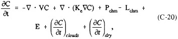
where C is the species volume mixing ratio, V is the three-dimensional velocity vector at each grid point in the model domain, Ke is the eddy diffusivity used to quantify the subgrid-scale fluxes due to subgrid-scale turbulence, Pchm and Lchm are gas-phase chemical production and loss terms, E is the emission rate, (![]() C/
C/![]() t)clouds is the time rate of change due
t)clouds is the time rate of change due

to cloud effects (including subgrid-scale vertical redistribution, aqueous chemical interactions, various nucleation and other droplet-related processes, and scavenging), and (![]() C/
C/![]() t)dry represents the rate of change due to dry deposition.
t)dry represents the rate of change due to dry deposition.
A general equation for calculating Qi, the concentration of the total aerosol mass in size category i, is given as:
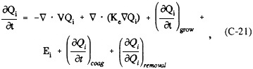
The term on the left represents the change in the total concentration of the airborne particle mass in size category i over time. The first term on the right refers to advection and the second to turbulent diffusion of the airborne particles. The growth term represents the change in concentration due to changes in thermodynamic equilibrium and nucleation of new airborne particles and condensation of vapor onto existing particles due to production of new material via gas-phase chemical reactions. The coagulation term represents the change in concentration due to coagulation of particles. The removal term represents the concentration change due to sedimentation, particle scavenging, and wet and dry deposition as well as the effect of cloud processing on the size distributions. Finally, Ei represents the change in aerosol concentration due to direct particulate emissions.
For the proper treatment of visibility issues, it is essential that the models include appropriate descriptions of the aerosol processes. Mechanistic visibility models should involve two separate components. First, chemically resolved airborne particle size distributions need to be calculated at specified grid points. Information is required on the characteristics of primary particle emissions as well as on atmospheric aerosol processes that affect further evolution of particle size distributions. Processes that must be considered include advection, diffusion, coagulation, evaporative shrinkage or condensational growth of particles, gas-particle chemical reactions, cloud processing, and wet or dry deposition. There is a close coupling between the formation of secondary particles,
which plays a major role in visibility impairment, and gas and in-cloud chemistry. Also, aerosol transport and removal by wet or dry deposition are dependent on local meteorology. Therefore, models that are used to determine airborne particle size distributions must be linked with meteorology and gas-phase chemistry models. Lorentz-Mie theory is used to calculate the optical characteristics of airborne particles by integrating over calculated particle size distributions. The particle-concentration prediction and the optical aspects of these computations involve mathematical approximations (introduced to speed up the calculations) and assumptions about the physical and chemical characteristics of atmospheric particles. These simplifications will affect the validity of calculated results. Therefore, the uncertainties associated with such model predictions need to be determined.
The phenomena that need to be considered in developing the aerosol models vary among the different chemical species. For example, although some sulfate particles are emitted directly by sources, most sulfate particles are formed in the atmosphere by the chemical transformation of SO2 gas. Reactions that lead to sulfate particle formation can take place either in the gas phase or in liquid particles or cloud droplets. The size distribution and therefore, the optical properties of the secondary sulfate particles depend on the chemical transformation mechanism. Organic particles can be either primary (directly emitted as particles) or secondary (formed from gas-phase organic substances), although the relative contributions of both remain poorly understood. The particulate nitrate, ammonium, and water content are determined primarily by thermodynamic equilibrium between particles and gas-phase species. All particles are influenced by removal processes, although the extent of wet removal processes will depend on hygroscopicity and particle size. An important practical issue in developing mechanistic visibility models is the assessment of the detail and accuracy with which such processes need to be described to achieve satisfactory results.
A variety of approaches has been developed for calculating the evolution of atmospheric particle size distributions. Several have been compared by Seigneur et al. (1986). The approaches differ in accuracy, computational speed, and ability to describe the behavior of multicomponent aerosol systems and internally and externally mixed particles. Each of these factors needs to be weighed in selecting the optimal model for a given application.
Proper characterization of the relationship between aerosol concentrations, the properties of the visual environment, and the effect on the public of changes in visual air quality is central to correct prediction of the effects of visibility protection programs. The relationship between aerosol concentrations as determined by models and human perception generally is based on optical principles. Most work to date is based on the assumption that particles are spherical and that particles consist of homogeneous mixtures. Lorentz-Mie theory is then used to calculate the scattering and absorption of light by individual particles. The total extent of particle scattering and absorption is determined by integrating over calculated particle size distributions that are chemically resolved. Although the assumption is often reasonable for submicron particles, little experimental work has been done to examine its validity. The effect of nonspherical particles on light extinction needs to be considered in areas where coarse dust and fly ash are important contributors to visibility reduction. The scattering and absorption of light by air and NO2, respectively, are straightforward calculations.
The optics calculations described above can be made for each of the grid points at which composition-dependent particle size distributions are calculated explicitly or implicitly by an air quality model. The calculations provide information on variations of atmospheric optical properties over the three-dimensional grid. Thus, for model calculations where particle size distributions are estimated, it is possible to use radiative transfer theory (Chandrasekhar, 1960) to calculate visibility indexes that depend on sight path, cloud cover and ground reflectance, color and texture of distant objects, and the angle between the observer and the sun, which requires data on the surrounding terrain and cloud cover. When composition-dependent size distributions are not calculated explicitly in the model, alternative approaches must be developed to link the aerosol composition information to optical factors. For example, in many field studies it has been observed that the atmospheric extinction coefficient per unit mass for certain airborne particle components (e.g., sulfate and elemental carbon particles) typically lies within a characteristic range of values. Those empirically determined extinction efficiency values could be multiplied by model predictions of aerosol species chemical concentrations to estimate the light-extinction coefficient that corresponds to a particular situation being modeled.
HYBRID MODELS
Hybrid models have been developed in the belief that no single mechanistic or receptor-oriented model can represent reality accurately under all circumstances and that each modeling approach has its own specific strengths and weaknesses. Hybrid (or composite) models offer the possibility of better resolution of source contributions by combining two or more receptor, trajectory, deterministic, or atmospheric chemistry models. For example, the multiscale source-receptor model suggested by Chow (1985) combines a regional scale trajectory model, a principal component analysis receptor model, a CMB receptor model, and an urban scale Gaussian dispersion model into a single composite modeling approach.
Linear-Chemistry—CMB Hybrid Models
Composite model research has been pursued because the current state of the art limits regulatory applications of conventional CMB receptor modeling to particulate matter that is directly emitted to the atmosphere. The remaining sulfate, nitrate, and organic compounds that are not attributed to primary emissions are classified as secondary substances and cannot be attributed to specific sources, thereby severely limiting conventional use of the CMB model in visibility studies.
If additional assumptions are made, hybrid CMB-atmospheric chemistry models can be used to extend conventional CMB modeling beyond the limits outlined in EPA's regulatory guidance. If one accepts the assumption that conversion of reactive gases (e.g., SO2) to secondary particles (e.g., SO42-) is complete and that the secondary substances have not been preferentially deposited en route to the receptor, secondary particles can be apportioned among contributing source types.
In real-world applications where conversion is not complete or the secondary particles are deposited during transport, CMB has been used only in research settings to quantitatively estimate secondary aerosol source contributions. Several investigators have proposed secondary aerosol hybrid receptor models that include SO2-to-sulfate transformation and deposition terms, but none of the models has undergone thorough validation study (Stevens and Lewis, 1987; Dzubay et al., 1988).
Lewis and Stevens (1985) proposed a hybrid model that typifies the current state of hybrid models developed as a direct extension of the chemical element tracer approach that forms the basis of CMB receptor modeling methods. In that model, the secondary sulfate concentration from a specific source ![]() is estimated as
is estimated as
where Mp is the mass concentration at the receptor of primary fine particles from the source, A is the ratio of the source mass emission rate for SO2 and fine particles, and T describes both the transformation of SO2 to sulfate in the atmosphere and its loss due to deposition at the earth's surface. A chemical reaction model is needed to specify the extent of conversion, T, of SO2 to form sulfate.
Mp can be estimated by CMB receptor model applications or by use of multiple linear regression analysis. Mp also can be estimated using source tracers such as deuterated methane (CD4) when the assumption is made that the tracer is associated uniquely with a specific source. Tracer applications are discussed below.
Lewis and Stevens theorize that these hybrid models are limited to distances of less than 200 km because of the following factors: (1) the concentration of source tracer elements used to estimate Mp must be above measurement detection limits; (2) particle fractionation effects during transport due to the differing size distributions of the chemical species must not occur; and (3) the estimate of plume age required to calculate T becomes less certain as the distance from the source increases.
Given those limitations, the principal assumptions inherent in the application of the hybrid model of Lewis and Stevens for secondary aerosol apportionment are as follows: (1) dispersion, deposition, and transformation processes are linear or pseudo-first-order processes in nature; (2) dispersion affects all three pollutants (SO2, sulfate, and Mp) identically; (3) dry deposition is the only form of deposition that occurs (wet deposition, and oxidation by aqueous phase and heterogeneous processes are excluded); (4) deposition affects all the fine particles in the same way, but the rate of deposition of SO2 might be different; (5) secondary sulfate is produced only by homogeneous gas-phase oxidation of SO2; and (6) plume age can be estimated from available wind data.
If the path of the air parcel can be computed by trajectory analysis, then plume age can be estimated more exactly.
Many real physical situations of interest may occur outside the bounds of the above assumptions (e.g., heterogeneous SO2 oxidation in clouds often is important).
A second type of composite model has been developed that employs CMB receptor modeling for attribution of primary airborne particles to their sources, accompanied by a separate deterministic model for sulfate formation and transport that is driven by atmospheric transport, reaction, and dilution calculations rather than by tracer concentration data (Harley et al., 1989). This approach employs the sulfate formation model of Cass (1981), which is based on gridded SO2 and primary sulfate emissions, hourly wind speed, wind direction, mixing height, dry deposition rates, and measured or computed atmospheric pseudo-first-order rates for conversion of SO2 to sulfates. The composite model has been applied to study the least-cost solution to the aerosol control problem in the Los Angeles basin (Harley et al., 1989).
Additional hybrid modeling can be envisioned in which tracer or CMB models are used for elements of the source attribution problem that are difficult to determine with a deterministic model (e.g., predictions of airborne soil-dust concentrations). More complete deterministic models for secondary airborne particle formation would then be used to compute sulfate, nitrate, and secondary organic particle concentrations along with those primary particle concentrations that are due to ducted emission sources.


