
5
Hydraulic and Tracer Testing of Fractured Rocks
Hydraulic and tracer tests are field methods for investigating fluid flow and chemical transport in the subsurface. They generally involve artificially inducing perturbations into the subsurface and measuring the resulting responses. In a hydraulic test the perturbation is created by injecting or withdrawing fluid from a borehole. The response is the change in fluid pressure in the same or nearby observation boreholes. In a tracer test a concentration perturbation is created by introducing a solute (tracer) into the subsurface. The movement of this solute is monitored by sampling for solute concentration at locations downstream from the tracer introduction point.
This chapter provides an overview of field techniques and methods of analysis and their advantages and limitations, but the intent is not to provide a manual for hydraulic and tracer testing. The discussion is limited to hydraulic and tracer tests under single-phase, isothermal flow conditions in which the solute concentration is sufficiently dilute that density effects can be neglected. Not covered are hydraulic and pneumatic tests for evaluation of the vadose zone. Hydraulic and transport properties are assumed to remain constant during the tests. In other words, it is assumed that coupling between fluid pressure and rock stress is negligible and that chemical reactions (such as precipitation) that alter fracture openings do not occur. These conditions are generally satisfied when testing at depths of less than a few hundred meters and when the induced pressure perturbation is relatively small (e.g., less than 10 bars). In contrast, the testing of deep petroleum or geothermal wells commonly involves large changes in fluid pressure to the extent that fractures are opened or closed. This coupling is addressed in Chapter 7, but it is beyond the scope of this report to discuss hydraulic tests in these settings.
The popular notion that hydraulic and tracer tests are methods to ''measure" hydraulic and tracer properties is somewhat misleading. In reality, the analysis of a hydraulic or tracer test is a modeling exercise consisting of two steps. The first step is to choose a model to represent flow and transport in the rock mass. In the petroleum industry this step is commonly known as the diagnostic phase. The choice of model is based on knowledge of the rock mass and the behavior of the test response. After a model is chosen, the second step is to determine values of model parameters such that model-computed responses match the field responses. This step is known as parameter estimation. If the model-generated response cannot be made to match the field response, the model must be revised. In other words, model selection and parameter estimation are an iterative process. In some cases there may be insufficient information to identify a unique model or a unique set of parameters for a given model. When faced with such nonuniqueness, several possible models and/or parameter sets may need to be considered until additional information is collected to better define the flow system. The hydraulic and transport properties determined from a hydraulic or tracer test are not unique. They must be considered within the context of the model chosen for analysis.
HYDRAULIC TESTS
In groundwater investigations, hydraulic tests are used to obtain estimates of hydraulic conductivity and specific storage of the aquifer medium. The term "transmissivity" refers to the product of hydraulic conductivity and aquifer thickness. "Storativity" is the product of specific storage and aquifer thickness. In the petroleum industry the properties obtained are permeability and total compressibility.
The distinction between hydraulic conductivity and transmissivity, or specific storage and storativity, is clear-cut when testing a porous medium, but confusion may arise in fractured rocks, as illustrated by the following example. Consider a rock mass containing a single extensive horizontal fracture bounded by impermeable rock. A borehole is drilled through this fracture, and a packer test is conducted in a test interval of length L containing this fracture (Figure 5.1a). If a porous-medium approach is used to analyze the test data and flow is assumed to be confined to a porous slab of thickness L (Figure 5.1b), a transmissivity T and hydraulic conductivity, K (= T/L), of the test interval can be calculated. For this particular example, however, the computed hydraulic conductivity is not representative of the rock mass because its value depends on the length of the test interval. If the length of the test interval is doubled (Figure 5.1c), the calculated hydraulic conductivity is halved. The transmissivity, however, is independent of the length of the test interval as long as no additional permeable fractures are encountered as the test interval is lengthened. To the extent that a single fracture can be viewed as an aquifer, it is useful to assign the transmissivity of the interval
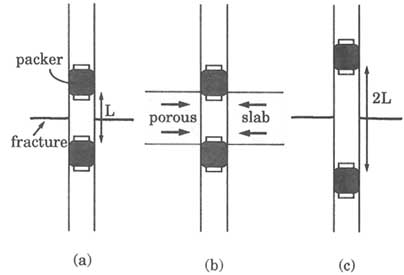
FIGURE 5.1 Packer test for determining transmissivity. (a) Packer interval of length L straddling a single fracture. (b) Packer interval of length L straddling a slab of fractured rock considered a porous medium. (c) Packer interval of length 2L straddling a single fracture.
to the fracture. Thus, fracture transmissivity is a term that is receiving increasing usage. The point of this example is not to discourage the use of hydraulic conductivity in test analysis but to emphasize the importance of reporting the test results with sufficient detail on the method of analysis so that readers are not misled.
Hydraulic Testing in a Single Borehole
In many subsurface investigations, particularly during the initial exploratory phase, hydraulic measurements (e.g., hydraulic head and flow rate) are restricted to individual boreholes. These tests are known as single-borehole hydraulic tests. Although single-borehole tests do not yield as much information as tests involving multiple boreholes, they offer the advantage of economy and speed. Single-borehole tests are commonly used for deep geological investigations because of the prohibitive expense of drilling multiple boreholes. Single-borehole tests are also used in some geotechnical investigations where time constraints preclude extensive testing with multiple boreholes.
Open-Borehole Versus Packer Tests
Single-borehole hydraulic tests can be performed in two configurations: in an open borehole or with packers. In an open-borehole test the entire uncased portion of a borehole is tested. Open-borehole tests are easy to set up and do not require expensive test equipment. They provide information on the hydraulic properties of the tested rock mass as a whole. They also provide valuable information for the design of packer tests, for example, on the expected range of pumping or injection rates. It is advantageous to conduct open-borehole tests prior to packer tests.
There are several disadvantages to open-hole tests. First, water inflow zones in the borehole cannot be located unless a flowmeter survey (Chapter 4) is conducted during pumping. Second, if the borehole penetrates several fractures or rock formations, the test response will be controlled by the most permeable zone, and little information will be obtained on the less permeable portion of the borehole. Third, when performed in low-permeability rocks, the test response may be dominated by wellbore storage effects (explained below), which complicate the interpretation of test data.
Packer tests utilize two or more packers to isolate a portion of the borehole for testing. Depending on the application, the test interval can vary from tens of centimeters to tens of meters in length. Packers can be used to isolate an individual fracture, a group of fractures, or an entire rock formation. In some test programs, a fixed test interval length is chosen, and the borehole is tested in consecutive sections throughout its length to obtain a hydraulic conductivity profile. Other test programs concentrate on testing only the more permeable portions of the borehole. In such cases the test intervals may vary in length, depending on borehole conditions as inferred from geophysical logs.
Test Procedures
The basic procedure of a single-hole hydraulic test is to inject or withdraw fluid from a test interval while measuring the hydraulic head in the same test interval. Prior to testing, borehole conditions are allowed to reequilibrate following installation of test equipment. Test equipment can be set up in many different ways, examples of which can be found in Zeigler (1976), Bennett and Anderson (1982), and Bureau of Reclamation (1985). In a packer test the hydraulic heads above and below the test interval are monitored to check for fluid leakage around the packers. Leakage can result from poor packer seals or the presence of "short-circuiting" fractures between the test interval and the rest of the borehole. When testing at depth, temperature in the test interval should be monitored because a change in temperature resulting from thermal disequilibrium (e.g., if the rock was cooled by drilling fluid prior to the test) can cause anomalous responses (see, e.g., Pickens et al., 1987).
During injection or withdrawal, the head change should be sufficiently large that the flow rate is measurable but not so large as to alter the hydraulic properties of the rock mass. A high injection head can open existing fractures and increase their transmissivities. In an extreme case, hydraulic fracturing can result. Conversely, a large reduction in head during fluid withdrawal can cause dissolved gas to come out of the solution. Gas bubbles lodged in fractures can reduce their transmissivities.
Five common procedures for single-hole hydraulic tests are discussed below: (1) constant-flow tests, (2) constant-head tests, (3) slug tests, (4) pressure pulse tests, and (5) drillstem tests. Figure 5.2 shows schematic plots of head and flow
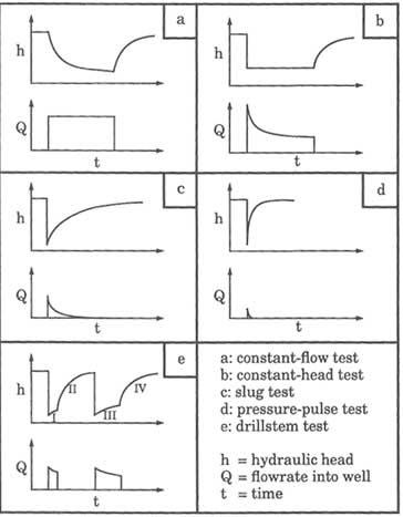
FIGURE 5.2 Schematic plots of hydraulic head and flow rate versus time for single-hole hydraulic tests.
rate versus time for these tests. Typically, the decision on which test to perform is based on the expected transmissivity of the test interval, the volume of rock to be sampled, and the availability of time and equipment. Test duration can range from 10 minutes in a geotechnical investigation to many days in a petroleum or water production test. Other factors being equal, a test of longer duration, involving a larger volume of injected or withdrawn fluid, will sample a larger volume of rock in the vicinity of the borehole. Quantifying the volume of rock sampled by these tests is a topic of current research.
The constant-flow pumping test (Figure 5.3), in which fluid is withdrawn at a constant rate from the test interval, is the most common test method in the
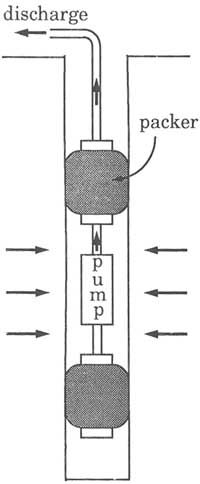
FIGURE 5.3 Equipment setup for a constant-flow pumping test in a single borehole.
groundwater and petroleum industries. Despite its popularity, this test is not without drawbacks. When performed with packers, the test is equipment intensive because a submersible pump must be used (Figure 5.3). Because most pumps operate over a limited discharge range, it is necessary to know the approximate transmissivity of the test interval in order to select the appropriate pump. Consecutive interval testing along a borehole becomes impractical, as the transmissivity variation from one test interval to another necessitates frequent changing of pumps. When testing an interval of low transmissivity, constant flow can be difficult to maintain and the pump can stall. For these reasons, constant-flow pumping tests are commonly reserved for testing more permeable intervals. An exception to this generalization occurs when testing in an environment where the hydraulic head is higher than the discharge point (e.g., in an underground facility, a naturally flowing well). In this case a constant outflow can be controlled by a flow regulator and a pump is not needed.
During a constant-head test (Figure 5.4), fluid is injected into or withdrawn from a test interval while keeping the head of the test interval at a constant value. Constant-head injection is common practice in geotechnical investigations. Constant-head withdrawal is practical when testing in an underground chamber. If the hydraulic head in the test interval is higher than the chamber floor, the test interval can be opened to free drainage. A key advantage of constant-head testing is that it generally presents no special technical difficulties when applied to test intervals of low transmissivity, as long as the flow rate is measurable. The effects of wellbore storage also are minimal, which simplifies data analysis.
A slug test (Figure 5.5) is performed by rapidly raising or lowering the fluid level in the pipe string or tubing connected to a test interval and monitoring its recovery to an equilibrium level. Typically, the test equipment includes a downhole valve in the test interval (Figure 5.5). After the packers are inflated, the test interval is isolated from the pipe string by closing the downhole valve. The fluid level in the pipe string is then raised or lowered by addition or removal of fluid. At the start of the test, the downhole valve is opened so that the hydraulic head in the pipe string is imposed on the test interval. If the fluid level in the pipe string were to be raised, fluid would drain from the pipe into the rock. If the fluid level was lowered, fluid would drain from the rock into the pipe. The downhole valve is kept open until the fluid level recovers to its equilibrium position. Slug tests are suitable for test intervals of moderate to low transmissivity. The test duration depends on the transmissivity of the test interval and the inside diameter of the pipe string. Lower transmissivities and larger pipe diameters lead to longer test times. Because pipe diameter can be varied, the duration of a slug test is controllable to a limited extent.
A pressure pulse test (Bredehoeft and Papadopulos, 1980) is similar in concept to a slug test, with the exception that the downhole valve is closed after the hydraulic head in the test interval is abruptly increased or decreased. The downhole valve is opened just long enough for the head in the pipe string to be
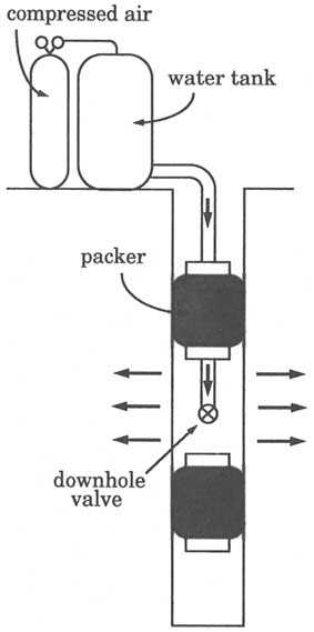
FIGURE 5.4 Equipment setup for a constant-head injection test in a single borehole.
transmitted into the test interval. Alternatively, the initial head disturbance can be created by using a hydraulic piston to inject a known volume of fluid into the test interval. The duration of a pressure pulse test depends on the transmissivity and the "system compressibility" of the test interval. System compressibility is
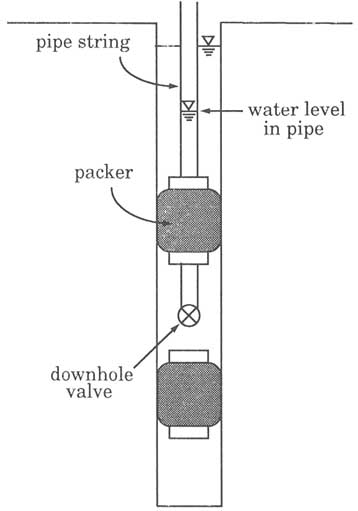
FIGURE 5.5 Equipment setup for a slug test in a single borehole.
a function of the fluid compressibility and the compliance of the test equipment (e.g., Neuzil, 1982). Because head recovery is controlled by compressibility effects rather than filling or draining fluid from the pipe string, the duration of a pressure pulse test is much shorter than that of a slug test, all other factors being equal. For this reason, the pressure pulse test is commonly applied to test intervals of very low transmissivity. However, the volume of rock tested by a pressure pulse test is significantly smaller than that tested by a slug test.
The drillstem test was originally developed in the petroleum industry for testing wells before casing is installed. The equipment for a drillstem test is similar to that for a slug test. After the packers are inflated, the downhole valve (known as the tester valve in the petroleum industry) is shut and fluid is removed from the pipe string. The actual test comprises four stages (identified as I, II, III, and IV in Figure 5.2e). The first stage is the initial flow period, when the tester valve is opened for five to 10 minutes, allowing formation fluid to enter the pipe string. During the second stage, which lasts about an hour and is known as the initial shut-in period, the tester valve is shut so that fluid pressure in the test interval can recover toward the undisturbed formation pressure. In the third stage the tester valve is opened for the final flow period of approximately an hour. This is followed by the fourth state, final shut-in period of one to two hours, when the tester valve is again closed and the pressure in the test interval is allowed to recover. The flow period of a drillstem test is equivalent to a slug test, and the test data can be analyzed in the same fashion.
Discussions of drillstem testing can be found in petroleum texts such as that by Earlougher (1977). Karasaki (1990) has proposed a variant of the drillstem test that consists of only one flow period, with the shut-in occurring at the time when the initial head drop has recovered by 50 percent. According to Karasaki, such a procedure improves the estimation of formation properties when a skin of low permeability (e.g., a mudcake) surrounds the wellbore.
Models of Single-Borehole Hydraulic Tests
Many common models of single-borehole hydraulic tests assume that the tested rock can be approximated as an isotropic homogeneous porous medium. Simple additions such as a highly transmissive fracture intersected by the borehole can be included in the analysis. The assumption of isotropy is made for a practical reason: reliable methods to characterize anisotropy generally require multiple boreholes. Homogeneity is assumed because the test response in a single borehole is insensitive to changes in hydraulic properties far from the test interval. Unless flow boundaries are close to the test interval, they are difficult to detect with confidence. For these reasons, models for single-borehole hydraulic tests are primarily concerned with fluid flow in the immediate vicinity of the test interval.
Flow in the vicinity of the test interval can be envisioned in terms of three basic geometries: spherical flow, radial flow, and linear flow. Combinations of these geometries are possible. The discussion of these geometries below assumes that flow is caused by pumping from the test interval, causing a drawdown in hydraulic head. To the extent that the head change is sufficiently small that the hydraulic conductivity is not changed, the discussion is equally applicable to an injection test, in which case the flow direction is merely reversed.
Spherical flow geometry describes fluid flow toward a spherical cavity in a homogeneous porous medium of infinite extent in all directions (Figure 5.6a). Equipotential surfaces are concentric spheres around the spherical cavity. When applied to hydraulic testing, the cavity can represent a short test interval, the length of which is not significantly greater than the borehole diameter (Figure 5.6b). Spherical flow is commonly characterized as "three-dimensional" because the hydraulic head varies in the three spatial dimensions.
Radial flow geometry describes flow toward a well that pumps from a homogeneous layer of infinite lateral extent (Figure 5.7a). This flow geometry serves as the model for a well test in a confined aquifer, which is bounded above and below by impervious materials. In the aquifer, equipotential surfaces are cylinders centered about the well axis. Thus, radial flow is also known as cylindrical flow. When applied to fractured-rock testing, the layer of porous medium represents a horizontal fracture zone or a single fracture bounded by impermeable rock (Figure 5.7b). Radial flow is commonly characterized as "two-dimensional" because the hydraulic head varies in the plane perpendicular to the well axis but remains constant along the direction parallel to the axis.
Linear flow geometry describes flow that is unidirectional, that is, flow that does not vary in space (Figure 5.8a). An example of linear flow is flow to a well that intersects a highly transmissive vertical fracture that extends a long distance
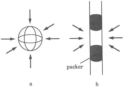
FIGURE 5.6 (a) Spherical flow to a cavity in a homogeneous porous medium. (b) Flow to a short test interval in a borehole that approximates spherical geometry.
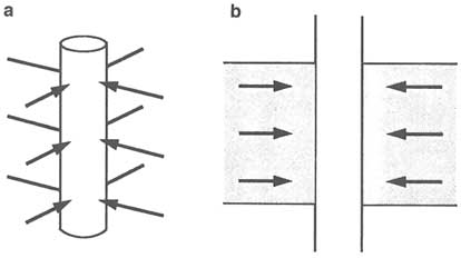
FIGURE 5.7 (a) Radial flow to a cylinder in a homogeneous porous medium. (b) Flow in a layer of porous medium confined above and below by impervious material.
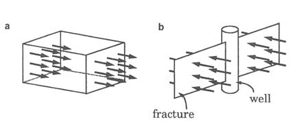
FIGURE 5.8 (a) Linear flow in a homogeneous porous medium. (b) Flow to a well that intersects a highly transmissive vertical fracture. The fracture acts as an extension of the wellbore.
from the well. The fracture acts effectively as an extension of the wellbore (Figure 5.8b), increasing its efficiency in extracting fluid from surrounding rock. Flow does not converge toward the well axis but is oriented in the direction perpendicular to the fracture plane. Equipotential surfaces are planar and parallel to the fracture plane. For this reason, linear flow is commonly characterized as ''one-dimensional" flow.
Combinations of the three basic geometries described above are possible, Figure 5.9 illustrates flow toward a test interval whose length is significantly
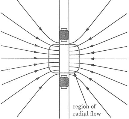
FIGURE 5.9 Radial-spherical flow. Flow is nearly radial close to the test interval and nearly spherical far from the test interval.
longer than the wellbore diameter in an infinite porous medium. In the vicinity of the test interval, flow is nearly radial, whereas far from the borehole, it is nearly spherical. Such a flow pattern is termed radial spherical. Another example of combined flow geometries is illustrated by flow to a well intercepting a highly transmissive fracture (Figure 5.10). Flow is nearly linear where the fracture intersects the wellbore. At a large distance away from the wellbore, flow is nearly radial. This flow pattern is termed linear radial.
Barker (1988) introduced the concept of a fractional flow dimension to hydraulic test analysis. This concept provides a novel approach to interpreting hydraulic tests. The fractional flow dimension describes the power relationship between the distance from the test interval and the area available for flow. For spherical flow the area (A) available to flow is 4πr2 (i.e., the area of a sphere of radius r), where r is the distance from the test interval. For radial flow, A =
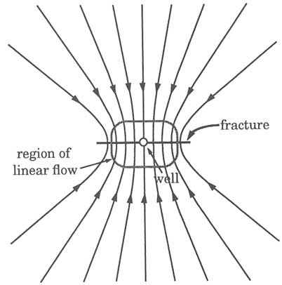
FIGURE 5.10 Areal view of linear-radial flow to a well intersecting a highly transmissive vertical fracture. Flow is nearly linear where the wellbore intersects the fracture and is nearly radial far from the well and fracture.
2πrb (i.e., the area of a cylinder of radius r and height b). For linear flow the area is a constant value independent of r. The relationship between A and r can be generalized as A = ![]() drd-1, where d is the Euclidean integer dimension (d = 1, 2, or 3), and
drd-1, where d is the Euclidean integer dimension (d = 1, 2, or 3), and ![]() d is a proportionality constant that is a function of d. In introducing the concept of fractional flow dimension, Barker allowed d to take nonintegral values. For example, a dimension between 2 and 3 represents a hybrid flow geometry between radial and spherical.
d is a proportionality constant that is a function of d. In introducing the concept of fractional flow dimension, Barker allowed d to take nonintegral values. For example, a dimension between 2 and 3 represents a hybrid flow geometry between radial and spherical.
The physical meaning of a fractional flow dimension is unclear, but Barker speculates that it describes a fracture network that exhibits fractal geometry. That is, the fractional flow dimension may be related to the fractal dimension of the fracture network. Polek (1990) showed that the flow network of such fractal objects is a subset of the geometric network. In the cases he studied, the flow
dimension, as determined by using Barker's (1988) approach, is less than or equal to the fractal dimension.
Mathematical analysis of models having the flow geometries described above is the subject of numerous papers in the groundwater and petroleum literature (e.g., Streltsova, 1988; Dawson and Istok, 1991). In many cases the models are sufficiently simple that analytical solutions can be found to the initial boundary value problem. The analytical solution is a mathematical formula that expresses drawdown and discharge as functions of time and model parameters. The availability of analytical solutions is highly advantageous for model selection and for gaining insight into how well model parameters can be estimated from field data.
Knowing the characteristic forms of the analytical solutions can be highly beneficial for selecting a flow model to analyze the hydraulic tests. For a constant-flow test a plot of the log of drawdown versus the log of time illustrates the contrasting behaviors for different flow geometries. Figure 5.11 shows the responses for the three Euclidean flow dimensions (n = 1, 2, and 3 for linear, radial, and spherical geometries, respectively). If the flow is spherical (i.e.,
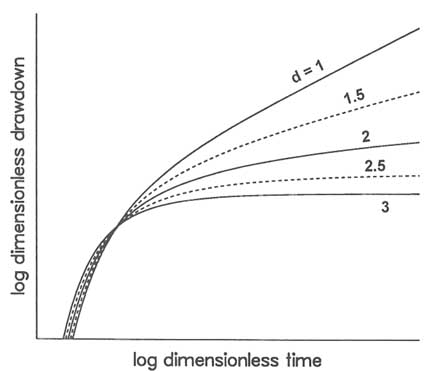
FIGURE 5.11 Plot of log dimensionless drawdown versus log dimensionless time for a constant-flow test. Numbers are flow dimensions. After Barker (1988), Figure 2.
d = 3), the drawdown initially increases with time but later approaches a constant value. If the flow is linear (i.e., d = 1), the drawdown plots as a straight line with slope 0.5 at late time. If the flow is radial (i.e., d = 2), the shape of the drawdown curve is intermediate between that of linear flow and spherical flow. For a constant-head test a similar comparison can be made by plotting the log of the inverse well discharge rate versus the log of time (Figure 5.12). Table 5.1 summarizes the characteristic behaviors of analytical solutions for different flow geometries.
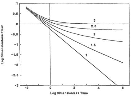
FIGURE 5.12 Plot of log dimensionless well discharge rate versus log dimensionless time for a constant-head test. Numbers are flow dimensions.
TABLE 5.1 Characteristic Behavior of Constant-Flow and Constant-Head Tests with Different Flow Geometries
|
Flow Geometry |
Constant-Flow Test |
Constant-Head Test |
|
Spherical |
Constant s at late time |
Constant Q at late time |
|
Radial |
s proportional to log t at late time |
1/Q proportional to log t at late time |
|
Linear |
s proportional to t1/2 at late time |
1/Q proportional to t1/2 during entire test |
|
|
||
Introduction of fractional flow dimensions has provided a new approach to hydraulic test analysis, but indiscriminant application of the method can lead to meaningless results. Because fractional-dimension-type curves can match a large range of hydraulic responses, there is a strong temptation to apply this analysis exclusively. In some cases a different interpretation may be more meaningful. For example, consider radial flow to a well in a two-dimensional flow system (such as a fracture plane) that is heterogeneous with respect to both transmissivity, T, and storativity, S. Suppose the well pumps from a local region of lower T and S (compared to their average values). In the vicinity of the pumping well, both T and S will appear to increase with radial distance from the well. If the hydraulic test is of a short duration, the well response will be controlled by the hydraulic properties of the near-well region. The response will be similar to that of a flow domain with a fractional flow dimension larger than 2. Conversely, if the well pumps from a local region of higher T and S, the response will be similar to that of a flow domain with a fractional flow dimension less than 2. The application of a fractional flow dimension model to analyze the test response in this example yields a flow dimension that is an artifact of the heterogeneity in the flow domain. To interpret this dimension as characterizing some scaling feature of the entire flow field is erroneous.
A final model discussed here is the double-porosity model, which was developed to describe flow in a fractured porous medium. Such a medium is assumed to comprise a network of fractures bounding intact porous blocks. The fractures have high permeability and low storage, whereas the blocks have low permeability and high storage. The fractures provide the pathways for flow to the well, and the blocks provide the main source of water. Figure 5.13 illustrates the drawdown behavior during a constant-flow test in a well with radial flow geometry. Initially, most of the pumped water comes from the fractures, and the head in the fractures drops rapidly (period A). As pumping continues, the blocks begin to supply water to the fractures, causing the head in the fractures to stabilize and the head in the blocks to drop (period B). As the heads in the fractures and blocks equalize, both systems produce water to the well, although the blocks are the dominant source (period C). The combined fracture-block response is operative for the rest of the test.
Estimation of Model Parameters
Parameter estimation is essentially a fitting procedure. After a model is selected, the model parameters (hydraulic properties) are adjusted until the model computed drawdown and flow rate match the field data. A steady-state analysis attempts to match only that portion of the field data collected after steady state is achieved. A transient analysis attempts to match the drawdown and flow rate for the entire duration of the test. Steady-state analysis is simple because parameter estimation reduces to the direct application of a simple formula to determine the
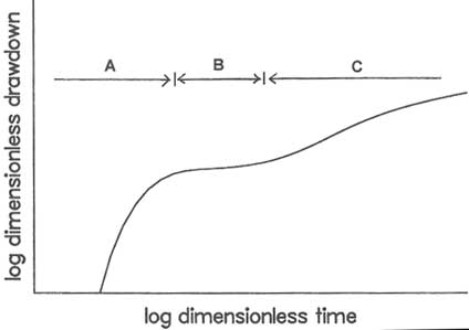
FIGURE 5.13 Plot of log dimensionless drawdown versus log dimensionless time for a constant-flow test with radial flow geometry for the double-porosity model. After Moench (1984), Figure 3.
hydraulic conductivity or transmissivity. However, the analyst must accept a number of assumptions (e.g., flow geometry), the validity of which may be uncertain. Transient analysis, although more complicated, offers the advantage that the flow geometry may be inferred from the field data.
It is somewhat ironic that steady-state analysis is generally applied to constant-head or constant-flow tests of relatively short duration (tens of minutes). Typically, the test is performed until both the flow rate and the hydraulic head in the test interval reach "stable" values, which is often taken to mean that the instrument readings do not change over several minutes. The stabilized head change and flow rate constitute the data from the test. If radial flow is assumed, the Theim formula (e.g., Bear, 1979) is used to compute the transmissivity of the test interval. For radial-spherical flow, formulas by Hvorslev or Moye yield the hydraulic conductivity of the rock in the vicinity of the test interval (Zeigler, 1976). Linear flow is generally not assumed in steady-state analysis.
Steady-state analysis is subject to errors from two sources. First, for tests of short duration, conditions may be far from steady state. Second, for certain flow patterns, a true steady state does not exist. Theoretical and field analyses show that the transmissivity or hydraulic conductivity determined from a steady-state analysis is often higher than the same quantity determined from a transient
analysis. Therefore, results of steady-state analyses should be considered as order-of-magnitude estimates.
Transient analysis can be done graphically or with computer software. The graphical method involves plotting the analytical solution and the data on separate sheets of graph paper and matching one to the other. The plot of the analytical solution is known as a type curve in the groundwater field, and the curve-matching procedure is known as type curve analysis. Recently, the use of automated computer analysis programs has gained popularity. The programs are based on regression techniques and are commonly set up so that the analyst can quickly try a number of different models. This interactive approach is desirable because the data may be matched equally well by type curves generated from different flow models. In such situations one may have to accept a range of hydraulic properties values until additional information becomes available to better guide selection of the flow model.
In principle, transient analysis yields the transmissivity and storativity if radial flow is assumed or hydraulic conductivity and specific storage if spherical flow is assumed. In practice, it is difficult to determine the storativity or specific storage with confidence from single-hole tests. During a constant-flow or constant-head test, storage effects are dominant only during the relatively short period (generally seconds to minutes) at the start of the test. The data during this period are commonly influenced by other factors, such as the inability to achieve constant flow or head instantly at the start of the test, that are neglected in the model.
In analyzing slug-test data, there is even greater uncertainty in determining storativity or specific storage because the analytical solutions for radial and spherical flow geometries are represented by a family of type curves. Figure 5.14 illustrates type curves for radial flow. Each curve corresponds to a different value of a dimensionless parameter that is a function of storativity and well geometry. For small values of storativity, the type curves are similar in shape, so it is difficult to obtain a unique match to the test data. A slight change of match from one type of curve to another can change the resultant storativity by an order of magnitude. The same problem occurs in the analysis of pressure pulse and drillstem tests.
To overcome the difficulty in selecting type curves, the method of matching to a derivative-type curve was introduced (Bourdet et al., 1989). The derivative-type curve is a plot of the derivative of the head with respect to the log of time against time (Figure 5.15). The shapes of derivative-type curves are somewhat more distinctive from one another and therefore provide an improved basis for curve matching. Test data must be of sufficient quality (i.e., accurate and free of noise) that their derivatives can be calculated for matching to the derivative curves.
Wellbore Storage and Skin Effects
Wellbore storage and skin effects are two factors that must be taken into account when analyzing single-borehole tests. Wellbore storage effect is due to
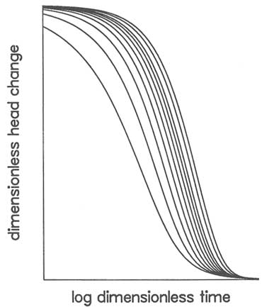
FIGURE 5.14 Plot of dimensionless head change versus log dimensionless time for a slug test with radial flow geometry. After Cooper et al. (1967), Figure 3.
the fact that, when the water level is lowered in an open borehole during the early part of a constant-rate pumping test, the actual rate of water removal from the formation is less than the pump discharge. If the rate at which water is removed from the wellbore is insignificant in comparison with the rate at which water is pumped from the formation, the wellbore storage effect is negligible. This is generally the case when testing highly transmissive aquifers. When testing low-permeability rocks, however, the pumping rate is generally low, and a significant portion of the pumped water may be derived from the wellbore. When wellbore storage dominates the test response, a plot of log drawdown versus log time is a straight line of unit slope. Neglecting this effect will result in erroneous interpretation of the hydraulic test. In packer tests the change in hydraulic head is not associated with a change in water level. Wellbore storage can generally
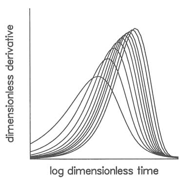
FIGURE 5.15 Plot of dimensionless derivative of head with respect to log of time versus log of dimensionless time for a slug test with radial flow geometry. Each curve corresponds to a different value of dimensionless parameter that is a function of storativity and well geometry. After Karasaki et al. (1988), Figure 4.
be neglected except when testing borehole intervals of very low transmissivity, in which case equipment compliance could create a wellbore storage effect.
The term skin effect was originally introduced in the petroleum literature to describe the change in permeability of the borehole wall as a result of drilling. The region of altered permeability is known as the skin, and the effect of the skin is described by a quantity known as the skin factor. If the permeability is reduced owing to invasion of drilling mud, the skin factor is positive and drawdown in the well during pumping is greater than drawdown in the absence of skin. If the permeability is increased because of well development, the skin factor is negative and drawdown is less than in the absence of skin. In fractured rocks where water or air is used as the drilling fluid, alteration of the borehole wall should be minimal. However, the highly heterogeneous nature of fractured rocks can give the impression of a skin effect. For example, if a borehole intersects a locally tight portion of a fracture, the region around the borehole may appear to
be surrounded by a positive skin. In general, independent information is needed to determine whether this effect is due to wellbore damage, formation damage, or testing of a low-permeability region.
The effects of wellbore storage and skin can be included in a model by specifying the appropriate boundary condition at the test interval. In many cases the two effects can be combined into a single dimensionless term that is a function of the storativity, skin factor, and the known geometry of the wellbore (Ramey et al., 1975; Sageev, 1986). As in the case of a slug test, a family of type curves exists for analyzing a constant-flow test with wellbore storage and skin effects (Figure 5.16), and the test data must be matched by using type curve analysis. Derivative-type curves also can be used to aid matching. For radial flow the test analysis yields the transmissivity and a quantity that is a function of storativity and skin factor. In general, the storativity and skin cannot be separately computed without additional information.
Hydraulic Testing with Multiple Boreholes
Multiple-borehole hydraulic tests are also known as interference tests or cross-hole tests. Like single-borehole tests, multiple-borehole tests can be per
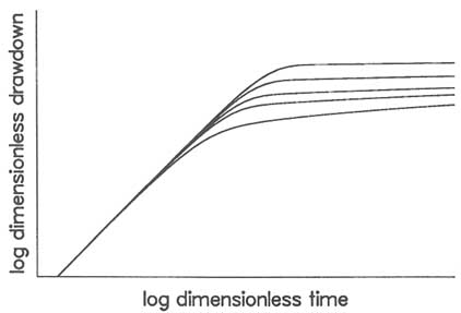
FIGURE 5.16 Plot of log dimensionless drawdown versus log dimensionless time for a constant-flow test with radial flow. Different type curves correspond to different values of a dimensionless parameter that is a function of storativity, wellbore storage, and skin factor. After Bourdet et al. (1989), Figure 1.
formed on open boreholes or on packer-isolated intervals. In the open-borehole configuration, fluid is pumped from one well and drawdown is observed in the pumped well and nearby observation wells. This is the traditional aquifer test in a groundwater investigation, or the interference test in the petroleum industry. When packers are used, fluid is pumped from a ''pumped interval" in one borehole, and drawdown is monitored in "observation intervals" in nearby boreholes. In testing rocks of low permeability, injection may be easier than pumping. For more permeable rocks, however, injection may be impractical because it requires a large source of water on the site.
Multiple-borehole tests offer a number of advantages over single-borehole tests. Multiple-borehole tests sample a larger volume of the rock mass. Consequently, the calculated value of the specific storage or storativity is subject to much less uncertainty. If the rock mass is treated as a porous medium, the anisotropy of the rock mass can be investigated. If flow is controlled by several highly transmissive fractures and the test objective is to characterize the interconnection between these fractures, multiple-borehole testing is indispensable.
Pumping at a constant rate is the common method to conduct multiple-borehole tests, but varying the pumping rate in a systematic fashion can be advantageous when hydraulic tests are affected by nearby activities such as well drilling, testing, or underground operations. If these disturbances obscure the response of the hydraulic test, data analysis will be very difficult. To remedy this situation, Black and Kipp (1981) proposed the "sinusoidal pressure test," which calls for varying the pumping rate or the hydraulic head in a sinusoidal manner. This strategy is similar to that of the "pulse test" in the petroleum industry (Johnson et al., 1966), where the pumping scheme consists of alternating periods of pumping and no pumping. The sinusoidal test causes the head response in the observation intervals to also vary in a sinusoidal manner. In the presence of interference by other activities, the sinusoidal response can be extracted from the hydraulic head data. However, the distance over which the test response can be observed in a sinusoidal test is generally less than that of a constant flow test. In actual application (e.g., Noy et al., 1988) the frequency of the sinusoid ranges from one to several cycles per day.
Test Procedures
The setup of a multiple-borehole test is highly dependent on the test objective and subsurface conditions. Because generalizations are difficult to make, the discussion below uses five examples to illustrate the different ways of setting up multiple-borehole tests for different conditions.
Example 1. A large, horizontal, areally extensive fracture is bounded by rock of sufficiently low hydraulic conductivity to be considered impermeable. A multiple-borehole test setup is illustrated in Figure 5.17. All the packer intervals contain the fracture, which is the sole feature that is investigated.
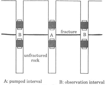
FIGURE 5.17 Example setup of a multiple-borehole hydraulic test in a rock containing a single extensive fracture.
Example 2. The rock mass bounding the large horizontal fracture in Example 1 is either permeable or contains a network of smaller fractures. In this case, pumping from the large fracture induces flow through the surrounding rock mass. The test setup shown in Figure 5.18 includes observation intervals to monitor drawdown and estimate hydraulic properties in the large fracture and the surrounding rock mass.
Example 3. A sedimentary rock, such as limestone or dolomite, contains highly transmissive horizontal fractures along bedding planes. These fractures are hydraulically connected by smaller vertical fractures, as shown in Figure 5.19. (A similar style of fracturing can occur in crystalline rock, although the large horizontal fractures may not be associated with bedding planes.) A multiple-borehole test in such a setting may call for pumping from one bedding-plane fracture and monitoring drawdown in the pumped fracture as well as in the overlying and underlying fractures.
Example 4. A densely fractured rock mass can be considered a porous medium. The systematic orientation of the fractures imparts anisotropy to the hydraulic conductivity. The test objective is to determine the hydraulic conductivity tensor of the rock mass, as opposed to the transmissivity of any individual
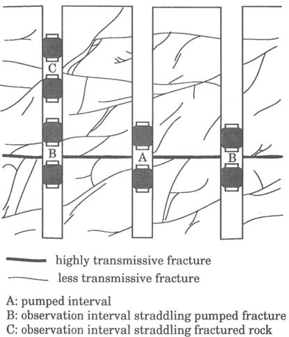
FIGURE 5.18 Example setup of a multiple-borehole hydraulic test in a rock containing an extensive and highly transmissive fracture with a network of less transmissive fractures.
fracture. As shown in Figure 5.20, the test setup involves pumping from a packed-off interval in one borehole and monitoring drawdown in observation intervals arranged in a three-dimensional pattern around the pumping interval.
Example 5. In this structurally complex setting, there are horizontal, inclined, and vertical fracture zones cutting through the rock mass, which is itself fractured (Figure 5.21). The greater complexity of this site, compared to the previous examples, requires a more extensive program of field characterization. A well-coordinated multidisciplinary approach is critical to its success. At an early stage, the investigation may be aimed at establishing the presence of the fracture zones.
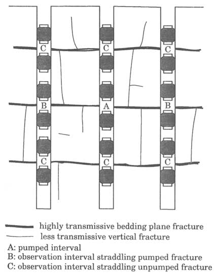
FIGURE 5.19 Example setup of a multiple-borehole hydraulic test in a rock containing highly transmissive horizontal bedding-plane fractures that are interconnected via less transmissive vertical fractures.
Identification of these zones requires extensive drilling, geological mapping, and geophysical investigations. Hydraulic tests may be limited to a single borehole or a few nearby boreholes. As a conceptual picture of the underground begins to emerge, full-scale, multiple-borehole tests, such as the one illustrated in Figure 5.21, can be conducted to investigate how the fracture zones are interconnected.
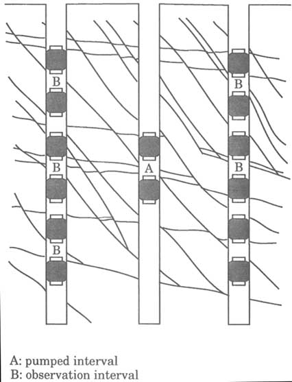
FIGURE 5.20 Example setup of multiple-borehole hydraulic test to determine the hydraulic conductivity tensor of a rock containing a dense and well-connected network of fractures.
Models of Multiple-Borehole Hydraulic Tests
Some models of multiple-borehole hydraulic tests can be adopted from models developed for porous media flow. For example, the single fracture in Example 1 above can be modeled as a thin confined aquifer, and the fracture in
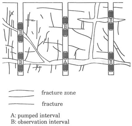
FIGURE 5.21 Example setup of a multiple-borehole hydraulic test in a rock mass with multiple sets of fractures and fracture zones.
Example 2 can be modeled as a leaky aquifer. (Leakage is a term used in groundwater hydrology to refer to the flow between an aquifer and an overlying or underlying layer of lower-permeability rock.) The multiple-fracture system in Example 3 can be treated as a multiple-aquifer system, with the bedding-plane fractures taking the role of the aquifers, and the rock layers (containing vertical fractures) taking the role of the aquitards. Models of this type have been developed by Hantush (1967) and Neuman and Witherspoon (1972). If the rock is treated as an anisotropic porous medium, as in Example 4, the method used to interpret the anisotropic permeability tensor from the well test data (see Appendix 5.B) developed by Hsieh et al. (1985) may be applicable.
To obtain analytical solutions to these models, homogeneity is generally assumed. (As noted earlier, the availability of an analytical solution is highly advantageous for analysis of test data.) Nonetheless, field experience indicates that fractured rocks are generally highly heterogeneous. In many cases, models
based on the homogeneity assumption are not capable of fully simulating the test response in fractured rocks. When testing in such an environment, the field hydrologist is commonly faced with test responses that are uncommon in porous media settings. For example, a nearby observation well may show no response, whereas a faraway well may show a large drawdown, even though these two observation wells lie along the same direction from the pumping well.
Accounting for heterogeneity of the rock mass requires a numerical model that is capable of simulating fluid flow through regions of variable hydraulic properties. To model a field setting such as that in Example 5, one approach is to use a numerical model (such as a finite-element model) that treats the fracture zones as highly transmissive elements and the fractured rock mass as porous blocks. Another approach may be the equivalent discontinuum model discussed in Chapter 6. At this level of analysis, there is little distinction between the methods discussed in this chapter and the modeling techniques discussed in Chapter 6.
Estimation of Model Parameters
If a model having an analytical solution is chosen to analyze the hydraulic test, the model parameters can be estimated either by type curve or automated computer matching. However, as noted earlier, the assumption of homogeneity required by the analytical solution is frequently inconsistent with the heterogeneous nature of fractured rocks. When faced with such heterogeneities, the analyst may be tempted to separately analyze the response in each observation interval as if the rock mass is homogeneous and isotropic. This approach yields a range of hydraulic property values, which are commonly interpreted as a qualitative measure of the heterogeneity of the rock. Such a simple approach is appealing, but it can be seriously wrong. Each separate analysis must be based on the assumption that the drawdown at the observation interval is due to the total rate of fluid removal at the pumping interval. However, in a heterogeneous formation, the low-permeability regions yield less fluid and consequently suffer lower drawdowns than higher-permeability regions. A separate analysis of observation intervals situated in low-permeability regions will yield erroneously high permeability values because the total fluid production is erroneously ascribed to a low drawdown. However, when the analysis assumes a heterogeneous rock mass, small drawdown correctly indicates relatively low permeability in the vicinity of the observation.
If a numerical model is used to analyze the hydraulic test, the analyst must decide on the parameterization of the model, that is, how to assign hydraulic properties to each cell or element of the model grid. On one extreme, each cell can have a different set of hydraulic properties. Such a "fine" zonation scheme is ideal for representing a highly heterogeneous rock mass, but the resulting model contains a large number of model parameters. On the other extreme, the
model grid can be divided into a smaller number of zones, with each zone having its own set of hydraulic properties. For example, a large region of rock mass may be lumped into a homogeneous zone, and major features such as highly transmissive fracture zones are treated as separate zones. Such a "coarse" zonation scheme does not represent all the details of the heterogeneity, but it results in a smaller number of parameters.
Parameter estimation for a numerical model amounts to choosing the model parameters such that the model-computed heads match the observed heads. This matching can be done by trial and error or by numerical inverse methods (e.g., Yeh, 1986). Computer programs that implement inverse methods are not yet widely available, but the modern approach to hydraulic test analysis in heterogeneous formations is clearly moving in this direction. Numerical inversion is faster than a trial-and-error approach and may provide a quantitative indication of the uncertainty of the estimated model parameters. The use of computer inversion programs allows the analyst to quickly try different parameterization schemes in order to select the most appropriate one.
For inverse methods there is a tradeoff between uniqueness and closeness of match (see, e.g., Carrera and Neuman, 1986). In general, the fewer the parameters in the model, the more likely they can be uniquely identified. On the other hand, fewer parameters limit the ability of the model to match certain field responses. Adding more parameters to the model may allow it to simulate a broader range of test responses, but the inverse algorithm may not be able to converge to a unique set of model parameters. The use of numerical inversion methods requires thoughtful judgments by the analyst. This topic is addressed further in Chapter 6.
TRACER TESTS
Tracer tests are generally applied (1) to explore connectivity in the subsurface and (2) to determine transport properties (e.g., kinematic porosity and dispersivity) and chemical reaction parameters, such as the distribution coefficient for mass transfer between liquid and solid phases (adsorption). In the first application (exploring subsurface connection), the approach is similar to that used for karst studies, where tracers are commonly used to investigate the possible connection between, say, a solution opening and a spring. The following discussion focuses on the second application, the determination of transport properties and chemical reaction parameters.
Solute Transport Processes
The discussion of tracer tests below is prefaced with a short review of key processes that control solute transport. Some of these processes are well known in porous media theory, for example, advection, dispersion, and adsorption.
Other processes, such as channelized transport and matrix diffusion, are concepts developed in the study of transport in fractured rocks.
Advection and Dispersion
The concepts of advection and dispersion in fractured rocks are identical to those in porous media. Advection refers to the movement of the tracer caused by the movement of the host fluid. When observed in detail, this movement is extremely complicated, as fluid velocity can vary on all scales: across the aperture of the fracture, in the fracture plane, from one fracture to another, and from one part of the fracture network to another part. To describe every detail of this movement would be impractical. In the classical approach to transport modeling, only the "average" velocity field is described. In concept, the average is taken over an appropriate volume, so small-scale variations are smoothed out. These averages represent the large-scale features of the velocity field. For example, the average velocity field may be uniform flow, radially converging flow to a pumping well, or recirculating flow from an injection well to a pumping well. The transport of tracer along this average flow field is referred to as advection.
Because the average velocity field does not capture all the details of the velocity distribution, advective transport does not fully describe tracer movement. The small-scale variations that are not described by the average velocity field will cause the tracer to spread and mix. When molecular diffusion is added to this spreading and mixing process, the result is what is commonly known as dispersion.
The classical approach assumes that dispersion can be treated as a Fickian (diffusive) process, but modern analyses suggest that this assumption is not always valid (Dagan, 1986; Gelhar, 1986). In a heterogeneous formation the solute must travel a certain distance before Fickian dispersion is established. Because tracer tests are commonly conducted over a relatively short distance, the validity of assuming Fickian dispersion remains an open question that awaits further research.
The magnitude of the dispersivity term depends on how much detail is known about the heterogeneity of the rock. If little is known about heterogeneity and the rock is modeled as hydraulically uniform, the dispersivity derived from a tracer test will appear to be large. If more is known and the rock is modeled as nonuniform, the dispersivity derived from a tracer test will be smaller.
Fracture Channels and Channelized Transport
Two processes have been recognized to be of special importance in fractured rocks. They are transport in fracture channels and channelized transport. A fracture channel is a long narrow region of enlarged aperture formed at the intersection of two fractures or by processes such as shearing (see Chapter 3). Transport
along enlarged fracture intersections could be significantly greater than transport along grooves on fracture planes. Channelized transport arises from the nonuniform velocity of fluid and solute transport in a variable-aperture fracture. Flow and transport are concentrated in narrow regions following pathways of least resistance.
The term channeling can refer either to transport in fracture channels or to channelized transport. Similarly, a channel can mean either a fracture channel or the narrow pathways of least resistance. However, Tsang and Tsang (1989) pointed out that transport in fracture channels is not the same as channelized transport. Fracture channels are fixed in orientation and position, whereas pathways of least resistance vary according to the flow direction. In addition, channelized transport does not require the presence of fracture channels. The computer simulation of Tsang and Tsang demonstrates how flow and transport tend to concentrate along narrow pathways in variable-aperture fractures (Figure 5.22). If the flow direction changes, the pathways of least resistance also change.
Diffusion into Stagnant Water and Rock Matrix
When flow is channelized in a fracture, significant portions of the fracture may be occupied by relatively stagnant or slow-moving water. Tracer moving through the channels can diffuse into this stagnant water. Tracer can also diffuse from the mobile water flowing in the connected fractures into the stagnant water residing in unconnected or dead-end fractures. Tracer can also diffuse from fractures into the rock matrix if the matrix has significant porosity. The net effect of these diffusive processes is a retardation of the apparent movement of the tracer compared to that of the water. As a general rule, the longer the duration of the tracer test, the more significant the effects of diffusion into stagnant water and rock matrix.
Adsorption
In the context of tracer testing, adsorption refers to the tendency of the solute to attach to solid phases in the host rocks. In a fractured rock, certain tracers can adsorb onto fracture surfaces, especially if the surfaces are coated with alteration products such as clay. The effect of reversible adsorption is similar to that of diffusion into stagnant water: the apparent movement of the tracer is retarded. If the tracer diffuses into the matrix and is adsorbed onto surfaces in the rock matrix, retardation can be greatly increased compared to that for adsorption on fracture surfaces. This is because the specific surface (i.e., adsorptive surface per bulk volume of rock) of the rock matrix grains is significantly greater than the specific surface of the fractures. Consequently, a larger quantity of tracer can be adsorbed on the rock matrix than on fractures.
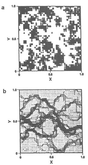
FIGURE 5.22 Computer simulation of channelized transport in a fracture with variable aperture. (a) Aperture distribution in the fracture plan. Lighter shading corresponds to larger aperture. (b) Flow rate distribution in the fracture plan, assuming constant-pressure boundaries on left and right and no-flow boundaries on top and bottom. Line thickness is proportional to the square root of the flow rate. From Tsang et al. (1991), Figure 5.
Field Methodology
A tracer test is conducted by introducing one or more chemicals (tracers) into the groundwater and measuring their concentrations over some time period at various sampling points downstream from the tracer introduction point. It is desirable to determine the distribution of the tracer in space and time, but this goal is usually not achievable. The number of sampling points (usually boreholes) is necessarily limited, so test data consist of concentration-versus-time curves (breakthrough curves) obtained at each sampling point.
The selection of tracers is a critical component in the design of tests. Using tracers with appropriate properties can help identify dominant transport mechanisms. Ideally, one of the tracers should move at the same velocity as the water. This tracer should be chemically inert during the course of the tracer test. That is, it should not decay, adsorb onto the rock, or react with other tracers. However, if diffusion into stagnant water or rock matrix occurs, even a chemically inert tracer will show an apparent retardation. In this regard, using several inert tracers with different coefficients of molecular diffusion can help quantify this effect. Adsorptive tracers can be used to investigate the sorptive properties of the fracture surfaces and rock matrix.
Natural Gradient Tracer Test
In a natural gradient tracer test, a tracer is injected into the groundwater system and is allowed to be transported by natural movement of the groundwater. The spatial distribution of tracer concentration is monitored by sampling from a grid of wells located down gradient from the injection point(s) (Figure 5.23). In general, water samples must be collected from different depths in each monitoring well to define the concentration distribution in three dimensions.
A natural gradient tracer test is perhaps the ideal method for the study of solute movement under natural or prevailing conditions because the prevailing groundwater condition is not disturbed, except for the brief period when the tracer is injected. From a theoretical point of view, the ability to define the spatial distribution of tracer concentration is highly desirable because such data allow direct calculations of tracer mass, velocity, and dispersion. For these reasons, several large-scale natural gradient tracer tests have been conducted in granular (e.g., sand) aquifers in recent years (e.g., Mackay et al., 1986; LeBlanc et al., 1991).
The natural gradient tracer test is generally expensive and difficult to apply in fractured rocks. In contrast to a granular aquifer at shallow depth, where multilevel samplers can be easily installed, fractured rock sites require numerous wells for sampling. Furthermore, tracer distributions in fractured rocks tend to be highly irregular. If, as some researchers argue (e.g., Tsang and Tsang, 1989; Abelin et al., 1991a,b), the tracer travels along channels that occupy small portions
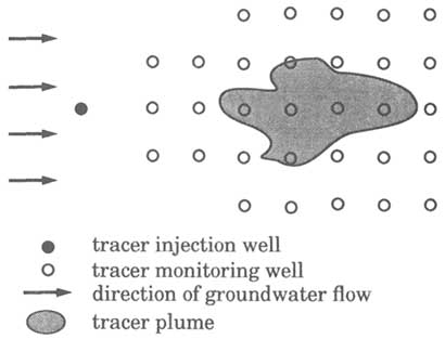
FIGURE 5.23 Setup of a natural gradient tracer test.
of the fracture planes, the tracer distributions in fractured rocks may resemble a braided network of one-dimensional pathways. In such a setting, sampling from a grid of wells may miss a significant portion, or even all, of the tracer mass.
Another problem with conducting a natural gradient tracer test in fractured rocks is the difficulty of collecting water samples that are representative of in situ conditions. This problem is especially severe for rocks of low permeability and porosity. In such setting, the extraction of water samples from tight fractures is a difficult task. Furthermore, the amount of water in the wellbore causes a significant dilution of in situ water. It is possible to back-calculate the concentration of in situ water from well-mixed wellbore water, but the result is inexact.
To obtain a representative sample of in situ water, it is necessary to purge the wellbore water by pumping for a period of time before collecting the sample. In a low-porosity formation, such pumping may significantly distort the flow field. Using packers to hydraulically isolate the fracture to be sampled will reduce the amount of purging required; however, standard packer equipment does not completely eliminate the problem of wellbore dilution. The development of specialized packer equipment (Novakowski and Lapcevic, 1994) to reduce well-bore volume would strongly enhance the ability to collect representative in situ water samples from fractures.
Divergent Flow Tracer Test
In a divergent flow tracer test, water is injected into a recharge well at a constant rate. After a steady flow field is established, the tracer is added into the recharge water either as a pulse or a step increase. The tracer concentration is then monitored at one or more wells in the vicinity of the recharge well (Figure 5.24). The advantage of this test is that the tracer is quickly forced into the flow system, so the test condition can be accurately represented by a simple mathematical model. In addition, if multiple sampling wells are used, a larger volume of rock can be investigated compared to the convergent flow tracer test discussed below. The disadvantages of the divergent flow tracer test are that a large water supply may be required for injection, the recharge water may clog the fractures, and the tracer is left in the rock at the end of the test. In addition, sampling from the monitoring well is subject to the same difficulties as discussed above: (1) the tracer may bypass the monitoring wells by flowing along channels
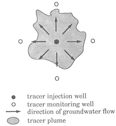
FIGURE 5.24 Setup of a divergent flow tracer test.
that are not intersected by or hydraulically connected to them; (2) the monitoring wells may intersect tight portions of fractures from which it is difficult to extract water samples; (3) when sampling from the monitoring wells, the in situ water may be strongly diluted by the wellbore water; and (4) in most cases there are not enough monitoring wells to allow calculation of the tracer mass in the subsurface.
Convergent Flow Tracer Test
In the convergent flow tracer test, water is pumped from a well until a steady flow field is established. A tracer is then injected, ideally as a pulse, into the flow system through a ''tracer injection" well (Figure 5.25). The arrival of the tracer at the pumping well is monitored by sampling the pumped water. This test avoids the sampling difficulties discussed above. Also, the amount of tracer recovered can be readily computed, and, under optimal circumstances, a large portion of the injected tracer is removed at the end of the test. However, injecting the tracer as a pulse into the flow system can be difficult to achieve. A common practice is to inject the tracer and then a certain volume of clean water. However, field experience suggests that such a practice does not flush all the tracer from
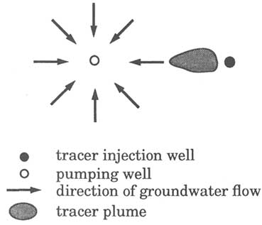
FIGURE 5.25 Setup of a convergent flow tracer test.
the borehole into the flow system. If some tracer remains in the borehole and slowly enters the flow system, the concentration-versus-time curve at the pumped well will have a long tail, which complicates the test analysis.
Because the convergent tracer test samples the relatively narrow flow region between the tracer injection well and the pumping well, it is desirable to introduce tracer at several injection wells to increase the volume of investigation. Simultaneous injection into several wells requires the use of different tracers that do not chemically interfere with each other. If the same chemical is to be used at different injection wells, the tracer from one injection well must be near fully recovered before the chemical is injected into another well. Such a sequential injection scheme will generally require onsite analysis of tracer concentration in the pumped water in order to determine tracer recovery. Appendixes 5.D and 5.E describe such tests.
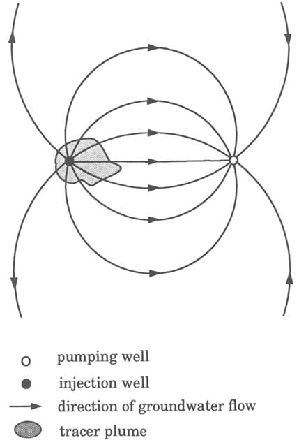
Two-Well Tracer Test
The two-well tracer test involves pumping from one well while recharging another well (Figure 5.26). Ideally, the pumping and recharge rates should be identical. In practice, however, the recharge rate is commonly less than the pumping rate owing to clogging of fractures. After a steady-state flow field (known as a doublet) is established, a tracer is added to the recharge water as a pulse or a step increase. Tracer arrival at the pumped well is monitored by sampling the pumped water. The two-well tracer test is attractive because the pumped water can be used as the recharge water, thus eliminating the logistical problem of obtaining an independent water supply for a divergent flow tracer test or disposing of the pumped water during a convergent flow tracer test. The main disadvantage of the two-well tracer test is in the analysis of data. In a doublet flow field, the travel time from the recharge well to the pumping well varies with the streamline along which the tracer travels. Thus, the shape of the breakthrough curve is primarily controlled by the different travel times of the tracer along different streamtubes and not by the dispersion in each streamtube. Consequently, the effect of dispersion is not as evident as in the convergent or divergent tracer tests. To improve the sensitivity to dispersion, Welty and Gelhar (1989) recommend that a pulse injection of tracer be used in this test, rather than a step rise in concentration.
Borehole Dilution Test
In a granular aquifer the borehole dilution test is a method for estimating the groundwater flow flux in the vicinity of a well screen. When applied to a fractured rock formation, the test yields the volumetric rate of groundwater flow through a packed-off interval of a wellbore. To conduct the test, a tracer is introduced into the packed-off interval of the wellbore and continually mixed.
The flow of groundwater into and out of the wellbore is allowed to flush out the tracer. By monitoring the tracer concentration in the wellbore with time, the volumetric rate of groundwater flow through the well can be determined.
Analysis of Tracer Tests
The analysis of a tracer test is similar to that for a hydraulic test. It requires the selection of a model (diagnosis) and the adjustment of model parameters until the model-computed breakthrough curves match the observed breakthrough curves (parameter estimation). For a model with an analytical solution, parameter estimation can be done by type curve matching in the same manner as for the hydraulic test. Although relatively uncommon in the past, the use of inverse methods to determine transport properties is likely to become more widespread.
Despite the similarity in their general approaches, tracer test analysis can be substantially more difficult than hydraulic test analysis. The greater difficulty arises from the fact that flow and transport processes respond differently to heterogeneities in fractured rocks. Dispersion and diffusion during fluid flow tend to smooth out the effects of heterogeneities. Solute transport during a tracer test is usually dominated by advection, which does not smooth out the effects of heterogeneities. Thus, in a heterogeneous formation, solute distribution tends to be significantly more irregular than the pressure distribution. This implies that the flow field or velocity distribution must be characterized in greater detail for transport modeling than for fluid flow modeling.
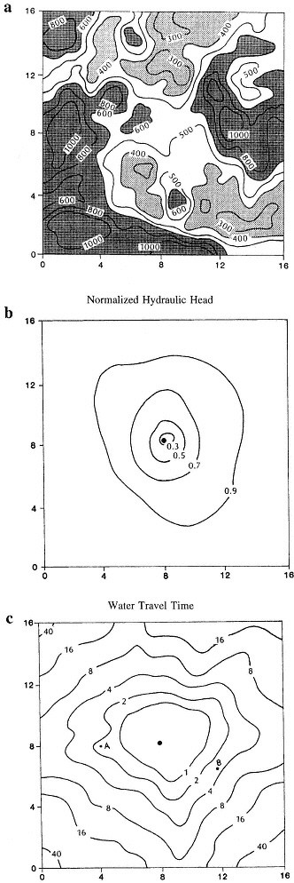
The unequal effects of rock heterogeneity on flow and transport are demonstrated by the computer simulation of Smith et al. (1987). Figure 5.27 a illustrates the aperture distribution in a rough-wall fracture, which forms one of the more dominant fractures in a three-dimensional fracture network. Figure 5.27b shows the head distribution that results when a well pumps from the center of the fracture plane. Although the lines of equal potential are not perfect circles (which would be the case if the aperture were uniform), their shapes are more or less circular. For this highly idealized case, one might conclude that even though the fracture is not uniform, representing it as having uniform properties would capture the main features of the hydraulic response. However, the same cannot be said for transport. Figure 5.27c shows the water (and tracer) travel time from any point in the fracture to the pump. Note that the travel times from different points at equal distances from the well can differ substantially. For example, the travel time from point A to the well is less than two time units, whereas the travel time from point B is almost four time units. For a fracture having a highly variable distribution of aperture, the variation in transport times may be even larger.
Despite the complexities of flow and transport in fractured rocks, simple models, which are derived from single- or dual-porosity media assumptions and are based on advection and Fickian dispersion, continue to be the popular choice for analyzing tracer tests. A good summary of these models is given by Welty
and Gelhar (1989). Recent advances that account for factors such as mixing in the wellbore are summarized by Moench (1989). Diffusion into the rock matrix can be incorporated by inclusion of an additional term into the transport equation, as shown by Maloszewski and Zuber (1985). A similar approach was used by Raven et al. (1988) to account for diffusion into stagnant water. The adequacy of using simple analytical models to analyze tracer tests in fractured rocks is open to question. Given the highly heterogeneous nature of fractured rocks, flow paths are likely to be highly complex, and therefore not well described by simple flow geometries such as those shown in Figures 5.25 and 5.26. Analyses based on simple models would likely lead to nonunique interpretations. A realistic analysis might require a numerical model to simulate flow and transport in a heterogeneous domain. The use of such models, however, would likely require extensive geological, geophysical, and hydraulic data as supportive information.
Some researchers have proposed to model the effects of channeling with a set of parallel one-dimensional transport models. The reasoning behind this approach is that, if the channels do not intersect each other, the transport in each channel can be analyzed separately as transport in a one-dimensional flow field. In addition, if the transport process in a channel can be modeled by classical advection and dispersion processes, analytical solutions are readily available. Thus, analysis of a breakthrough curve amounts to separating it into a number of component curves, each of which represents transport through a separate channel. By fitting an analytical solution to each component curve, the average velocity, dispersivity, and a dilution factor for each channel can be calculated. The dilution factor accounts for the portion of the injected tracer that enters the channel.
The separation of breakthrough curves into component curves has gained popularity because the procedure provides a simple way to analyze tracer test data that are not amenable to analysis using standard advection-dispersion models. For example, breakthrough curves for some tracer tests in fractured rocks show multiple peaks. By invoking the channel model, the individual peaks can be attributed to transport through individual channels (Figure 5.28a). A similar approach can be applied to breakthrough curves having very long tails. In this case the long tail is attributed to tracer transport along channels with successively lower velocities (Figure 5.28b).
A weakness of the channel model is that a certain degree of arbitrariness can be required in its application and interpretation. This is especially evident when analyzing breakthrough curves with long tails, which can be broken down into nonunique combinations of component curves. These component curves do not necessarily represent transport through actual channels in the fractures. Furthermore, even if the hypothesized channels are realistic representations of flow paths in the rock, these channels are particular to the flow geometry of the tracer test. In a different flow geometry, different channels will develop. It is as yet unclear how the characterization of channels in one flow geometry can be used
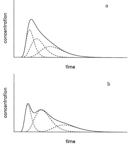
FIGURE 5.28 Separation of a breakthrough curve (solid line) into component curves (dashed lines). (a) Single peak case. (b) Multiple-peak case.
to characterize transport in a different flow geometry. Theoretical development in this area would significantly advance the interpretation of tracer tests in fractured rocks.
Research Needs
The highly heterogeneous nature of fractured rocks remains a major source of difficulty in modeling solute transport. A major research need is to develop
approaches to deal with this heterogeneity. Simple models based on uniform properties can frequently be calibrated to match the breakthrough curve from a single sampling point, but they are likely to fail in a calibration attempt that involves multiple breakthrough curves from several sampling points. In this regard the development of efficient numerical models of solute transport, coupled with parameter estimation algorithms, will greatly facilitate the analysis of tracer tests.
On a theoretical level, the development of alternative approaches that are not based on the classical advection/Fickian dispersion model may lead to new solutions. An example of such an approach, based on stochastic fracture networks, is discussed in Chapter 6. Another development that may lead to useful results is the solute flux approach advocated by Dagan et al. (1992). In this approach the variable of interest is the mass of solute discharged through a control surface. The control surface may be a wellbore, the discharge area of a groundwater flow system, or a compliance surface at some distance from a waste disposal site. Because the quantity of interest is found by integrating the mass flux across the entire surface, the result may be subject to less uncertainty compared to point concentrations.
On a practical level, the development of improved tools for in situ sampling would enhance the execution of tracer tests. In particular, packer equipment that minimizes the wellbore volume will substantially improve the ability to sample in situ fluid while reducing the need to pump a large volume of fluid to purge the well. Such equipment has been developed and used at the Grimsel test site in Switzerland (see Appendix 5.G). However, the most significant advancements in field methods will likely come from remote detection of the tracer distribution in the rock mass. The use of electromagnetic tomography to map the location of a salt solution is currently limited to two-dimensional cross sections. Three-dimensional images can, in principle, be obtained from a large number of two-dimensional cross sections. There are, however, practical and cost limitations. If the three-dimensional distribution of solute can be visualized, there is a much better chance of describing its movement.
Appendix 5.A
EXAMPLE OF A CONDUCTIVE NETWORK EXHIBITING FRACTAL GEOMETRY
The key concepts of a fractal object are scaling and dimension. Scaling implies that the small-scale features of the object appear in some sense like the larger-scale features (self-similarity or self-affineness). The dimension of a fractal object can take on nonintegral values. To understand these concepts, consider the two networks of conductive elements in Figure 5.A1. The left network is a regular Euclidean network. The right network approximates a fractal network, known as a modified Sierpinski gasket. (The smaller conductive elements are not shown.) The scaling feature of this fractal network is evident. Now assume that a well pumps from the center of each network. At a distance r from the well, the "area" available to flow can be determined by drawing a circle of radius r centered at the well and counting the number of conductive elements intersected by the circle. For the regular Euclidean network, the number of conductive elements intersected by the circle is linearly proportional to the radius r. In terms of the area-distance relationship, A = ![]() drd-1; the exponent d - 1 is unity. The flow dimension of this network is 2, which is consistent with the standard notion of Euclidean geometry. For the fractal network, however, the number of conductive elements intersected by the circle of radius r is proportional to r0.59. The flow dimension in this network is 1.59. Compared to the Euclidean network, the lower dimension of the fractal network is due to the fact that as the circle increases in radius it encounters successively larger regions without conductive elements. In this sense the fractal network can be viewed as a partially connected network of conductive elements.
drd-1; the exponent d - 1 is unity. The flow dimension of this network is 2, which is consistent with the standard notion of Euclidean geometry. For the fractal network, however, the number of conductive elements intersected by the circle of radius r is proportional to r0.59. The flow dimension in this network is 1.59. Compared to the Euclidean network, the lower dimension of the fractal network is due to the fact that as the circle increases in radius it encounters successively larger regions without conductive elements. In this sense the fractal network can be viewed as a partially connected network of conductive elements.
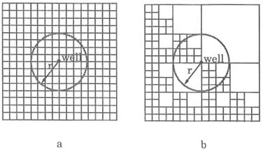
FIGURE 5.A1 Two networks of conductive elements. (a) A Euclidean network of dimension two. (b) A fractal network (modified Sierpinski gasket) of dimension 1.59.
APPENDIX 5.B
USING A MULTIPLE-BOREHOLE TEST TO DETERMINE THE HYDRAULIC CONDUCTIVITY TENSOR OF A ROCK MASS
If a fractured rock mass is viewed as a homogeneous anisotropic porous medium, the hydraulic conductivity is a second-order symmetric positive-definite tensor with six independent components. Determining these components will require testing with a relatively short pumping interval, so that, in the absence of boundaries, spherical flow will be established in the vicinity of the pumped interval. In theory, data from a minimum of six observation intervals, arranged in a three-dimensional pattern around the pumped interval, are needed. In field applications, where the assumption of homogeneity is not strictly satisfied, additional observation intervals are required so that the hydraulic conductivity components can be determined statistically. The test data are analyzed to compute the directional hydraulic diffusivity (directional hydraulic conductivity divided by specific storage). If the rock mass can be represented as a homogeneous porous medium, a three-dimensional plot of the square root of the directional hydraulic diffusivity versus direction should form an ellipsoid. If the directional hydraulic diffusivities fluctuate so severely that they do not form an ellipse in any meaningful sense, this is a direct indication that the tested rock does not behave as a homogeneous porous medium. This criterion is similar in concept to that proposed by Long et al. (1982). However, because of the difference in flow geometry, the two criteria may not be identical.
A hydraulic test conducted in the Oracle granite north of Tucson, Arizona, illustrates this application (Hsieh et al., 1985). The test was conducted in three boreholes—H-2, H-3, and H-6—drilled in a triangular pattern. The distance between boreholes ranged from 7 to 11 m. Figures 5.B1 a–c show the square roots of directional hydraulic diffusivities (dots) and the cross sections of the fitted ellipses along vertical planes between well pairs. Figure 5.B1 d is an oblique view of the cross sections oriented in three dimensions. Figure 5.B1 e is an oblique view of the fitted ellipsoid. Although the directional hydraulic diffusivities show a scatter owing to nonuniformities in the local rock properties, their square roots can be fitted to an ellipsoid. This result suggests that the tested rock behaves hydraulically in a manner not too different from that of a homogeneous anisotropic porous medium.
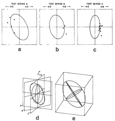
FIGURE 5.B1 Hydraulic conductivity ellipsoid determined by multiple-borehole testing in the Oracle granite north of Tucson, Arizona. (a)–(c) Polar plots of square roots of directional hydraulic diffusivities (dots) and cross sections of the fitted ellipse along vertical planes between well pairs. (d) Oblique view of cross sections (a) through (c). (e) Oblique view of filled ellipsoid. From Hsieh et al. (1985), Figure 12.
APPENDIX 5.C
USING A NUMBERICAL MODEL AND INVERSE METHOD TO ANALYZE A MULTIPLE-BOREHOLE HYDRAULIC TEST
Detailed subsurface characterization of a 200 m × 150 m × 50 m block of monzonitic gneiss at the Chalk River Nuclear Laboratories in Ontario, Canada, revealed the presence of four fracture zones (Raven, 1986). As shown in Figure 5.C1, fracture zone 1 is nearly horizontal and extends throughout the site; fracture zones 2 and 3 are, respectively, horizontal and inclined and cover only part of the site; and fracture zone 4 is vertical. The rock mass itself also is fractured and permeable. A multiple-borehole hydraulic test was conducted by pumping from well FS-10 and monitoring hydraulic heads in packer-isolated intervals in the other wells.
Carrera and Heredia (1988) modeled this site by using a finite-element model in which the fracture zones were explicitly modeled as two-dimensional planar features and the rock mass was represented as a continuum. To maintain a small number of model parameters, homogeneity was assumed in each fracture zone and in the rock mass, although hydraulic properties could differ from one zone to another. The initial model consisted of nine parameters, which were estimated by using a numerical inversion program. Subsequent revisions of the initial model included dividing fracture zone 1 into two homogeneous subzones and increasing the hydraulic connection between fracture zones by allowing higher hydraulic conductivities to occur at local regions in the rock mass between fracture zones. The final model, consisting of 13 parameters, yielded computed drawdowns that closely matched the observed drawdowns. Carrera and Heredia (1988) concluded that, even though single-borehole tests showed that the fracture zones are highly heterogeneous, the assumption of homogeneous fractures is adequate for modeling
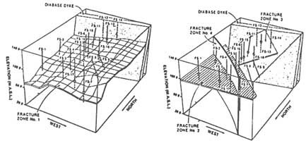
FIGURE 5.C1 Fracture zones in a block of monzonitic gneiss at the Chalk River Nuclear Laboratories in Ontario, Canada. From Raven (1986).
multiple-borehole hydraulic tests. This implies that the head distribution in the flow system is primarily controlled by the contrasting hydraulic conductivities of the fracture zones versus that of the rock mass. The internal variation of hydraulic conductivity in a fracture zone or in the rock mass has little effect on the observed flow pattern.
APPENDIX 5.D
A RADIALLY CONVERGENT FLOW TRACER TEST IN A FRACTURED CHALK FORMATION
A radially convergent flow tracer test performed by Garnier et al. (1985) illustrates the importance of matrix diffusion and adsorption. The test was performed in a fractured chalk formation approximately 9 m thick, from which a well pumps at a rate of 20.8 m3 per hour. Four tracers (deuterium, uranine, iodine, and carbon-13) were injected simultaneously into the same borehole as a concentrated pulse at a distance of 10.22 m from the pumping well. The observed breakthrough curve at the pumping well is shown in Figure 5.D1. The concentration of each tracer was normalized by their respective injective masses to allow for comparison.
If the four tracers all behave in the same way during transport, their normalized breakthrough curves will be identical. Figure 5.D1 shows that this is not the case. Of the four tracers, uranine has the largest molecular weight and therefore the lowest coefficient of molecular diffusion. A relatively small diffusion into the chalk matrix can account for the high peak of the uranine breakthrough curve. In contrast, the lower peaks for deuterium and iodine can result from their higher coefficients of molecular diffusion and therefore greater diffusion into the chalk
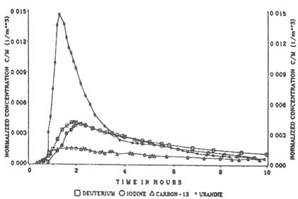
FIGURE 5.D1 Breakthrough curves of four tracers during a radially converging flow tracer test performed by Garnier et al. (1985). From Maloszewski and Zuber (1992), Figure 5.
matrix. Finally, the very low peak of carbon-13 suggests that it was lost by adsorption in the matrix.
To analyze this tracer test, Maloszewski and Zuber (1990) developed a one-dimensional transport model that accounts for advection, Fickian dispersion, matrix diffusion, and matrix adsorption that involves both an instantaneous equilibrium reaction and a nonequilibrium kinetic reaction of the first order. Calibration of the model yielded a fracture porosity of about 0.3 percent, a matrix porosity of about 40 percent, and a dispersivity of about 200 cm.
APPENDIX 5.E
A LARGE-SCALE FLOW AND TRACER EXPERIMENT IN GRANITE
Between 1984 and 1987, a large-scale flow and tracer experiment was performed by I. Neretnieks and co-workers in the Stripa Project mine in Sweden. Because the mine is situated beneath the water table and is kept at atmospheric pressure, it acts as a sink to which groundwater discharges. The experiment took place in an underground site that consisted of a 75-m-long main drift and a crossing arm 25 m in length. To measure the rate and distribution of this inflow, the entire ceiling and the upper part of the walls were covered with nearly 380 plastic sheets, which were used to collect water seeping from the rock (Figure 5.E1). For a period of over one and a half years, nine different tracers were injected continuously into nine intervals in three boreholes drilled vertically upward from the ceiling of the main drift. Tracer concentration was sampled from the plastic sheets for more than two years.
The results of this experiment, reported by Abelin et al. (1991a, 1991b), illustrate the complexities encountered in the analysis of solute transport in fractured rocks. The heterogeneity of the flow system can be observed in the highly uneven distribution of the water inflow rates, the highest occurring near one end of the crossing arm. The tracers, however, emerged in the central part of the main drift. Of the nine injected tracers, three were not detected during the course of the experiment. Of the tracers that reached the drift, recovery varied from 2.8 percent to 65.8 percent. The less-than-complete recovery may be due to the movement of tracers into pathways that do not lead to the drift and the
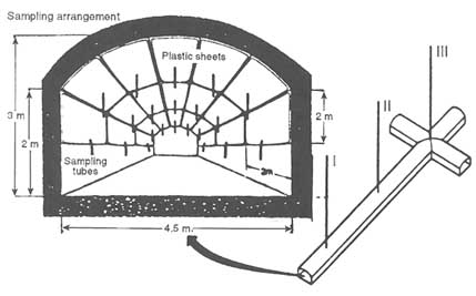
FIGURE 5.E1 Underground site in Stripa Project mine where a large-scale flow and tracer experiment was performed. From Abelin et al. (1991a), Figure 2.
diffusion of tracers into regions of stagnant water. The first possibility was verified by the detection of a tracer in a nearby drift of the Stripa mine complex. The complex's flow system suggests that knowledge of the groundwater hydraulics and flow paths is critical for the design and analysis of tracer tests in fractured rocks.
APPENDIX 5.F
DIAGNOSTIC WELL TEST ANALYSIS AT THE FRACTURE RESEARCH INVESTIGATION
The Fracture Research Investigation (FRI) in the Grimsel Rock Laboratory, which is located in the Alps in southern Switzerland, provides an excellent example of diagnostic well test analysis. A hydrologically active and accessible fracture zone was selected for investigation, and five studies were jointly undertaken (Majer et al., 1990). A detailed geological investigation provided background information. Extensive cross-hole tomographic studies imaged the fracture zone, which was observed crossing two parallel drifts. Hydrological tests were designed based on the results of the geological and geophysical investigations.
Hydraulic tests were planned in two boreholes drilled from the two drifts using the 1987 tomography results (Figure 5.F1). Each test consisted of pumping water in a given interval at a constant pressure and monitoring in all the other intervals. Test 1 was undertaken to provide a hydrological characterization of the main fracture zone that was identified in the tomographic images (feature A in Figure 5.F1). Packers were placed such that they confined the main fracture zone as tightly as possible in order to minimize wellbore storage and isolate the hydrological system (Figure 5.F2). This isolated interval (interval I1.2) was used as the inflow interval, and pressure was monitored in all the other intervals. Based on these results (Wyss, 1988), feature A is clearly the most significant hydrological feature at the FRI site.
Figure 5.F3 shows the pressure transient interference data at various observation points during Test 1. Note that the interval I3.1 responded most markedly during pumping. The response data at I3.1 are compared to the theoretical response in Figure 5.F4. As can be seen from the figure, the pressure observed at I3.1 is significantly lower than predicted by the analytical solution, although the shapes of the curves are almost identical. The analytical solution assumes that the fracture is infinite, isotropic, and homogeneous. Therefore, conditions must exist where one or more of the above assumptions are not appropriate. A number of violating conditions may exist, including:
-
Skin: there is a low-permeability zone around the injection well, that is, a skin that causes the effective pressure at I1.2 to be lower.
-
Anisotropy: the fracture is anisotropic, and the maximum permeability direction is oriented vertically.
-
Leakage: there is leakage from the fracture to the adjacent rock, so the pressure is more dispersed.
-
Boundary effect: the boundary effect of the laboratory tunnel keeps the pressure low in I3.1.
Skin effect is usually suspected when an anomalous result is obtained. However, the flow rate curve (not shown) does not match any of the skin curves, and
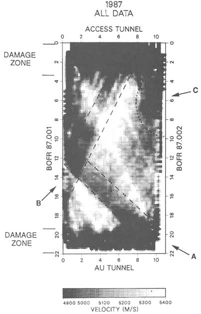
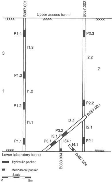
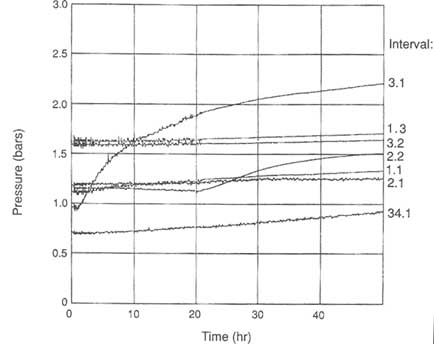
FIGURE 5.F3 Interference buildup data for test 1 at various observation points. From Majer et al. (1990).
the match for I3.1 is not very good. Therefore, it seems that the conventional skin effect cannot explain the observed behavior. Alternatively, if a constant pressure drop independent of the flow rate is assumed at the borehole wall, the flow rate curve would not exhibit the skin effect. Although the no-skin curve is closer to the observed curve, it still does not explain the observed inflection in the flow rate curve.
Geological observations indicate that the fracture zone may be highly anisotropic with the highest permeability in the vertical direction. Thus, injected water may flow preferentially in the vertical direction. As a result, the observed pressure head in the horizontal direction in interval I3.1 may be lower than for the isotropic case. Analytical solutions for flow to a well in an anisotropic medium can be obtained through a transformation of coordinates (Kucuk and Brigham, 1979). However, an unreasonably large anisotropy ratio (2 × 10⁹) is necessary to explain the pressure drop. Therefore, it is unlikely that anisotropy is the sole cause for the low-pressure measurement.
As can be seen from Figure 5.F3, small interference responses were observed at various intervals that are not in the plane of the fracture zone. This implies
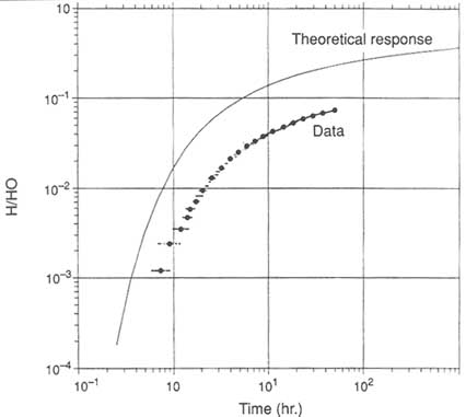
FIGURE 5.F4 Comparison between interference buildup data for test 1 and the theoretical response curve. From Majer et al. (1990).
that there is leakage from the fracture zone into adjacent rocks, which may explain why the interference response in I3.1 was low. The solution for pressure in a constant-pressure test in a leaky aquifer is not readily available in the literature. However, if the thickness of the rock into which leakage occurs is assumed to be of finite size and the leakage is at quasi-steady state, the solution presented by Da Prat et al. (1981) for a double-porosity medium can be used. The match between the flow rate data and the Da Prat solution (not shown) is very good, but the match between the pressure data and the solution in I3.1 (not shown) is poor. The theoretical pressure is too high compared to the data because in the model the rock is assumed to be of finite size.
Leakage into an infinite-sized rock was considered through a Laplace space solution for the normalized pressure in the fracture zone at a nondimensional distance, rD, under a constant-pressure test with leakage into an infinite-sized rock. Values of drawdown and flow for the Laplace space solution are plotted in Figures 5.F5 and 5.F6 for various combinations of fracture and matrix proper-
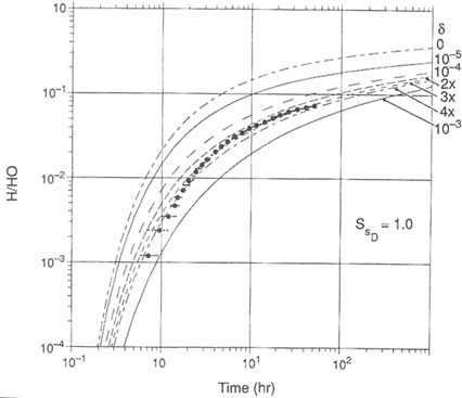
FIGURE 5.F5 Comparison of drawdown and flow for leakage into an infinite-sized rock with data from I3.1. From Majer et al. (1990).
ties. Also plotted are the observed data. The match with the interference data in I3.1 is much better than in Figure 5.F4. However, the match between the data and the theoretical curves at long times is not good. In particular, the observed flow rate data are much flatter than the theoretical curves at long times (Figure 5.F6).
Nonetheless, the concept of leakage appears to explain the trend of the data: low interference pressure and flattening of the flow rate curve at long times. The weak hydraulic connection between I1.2 and I2.2 may be through this low-permeability rock matrix. It is worth noting that the 1988 seismic tomography results (Figure 5.F1) indicate the existence of a feature (feature B) that extends diagonally from the access tunnel toward borehole 87.001. This may be a conduit for the leaking water. This localized leakage is not taken into account by the analytical solution; it could explain the low pressure in I3.1 and the flattening of the flow rate curve.
Hydraulic tests have confirmed the hydrological significance of this fracture zone, which was previously identified by seismic tomography. It appears that the majority of flow occurs in the relatively thin fracture zone that connects I1.2
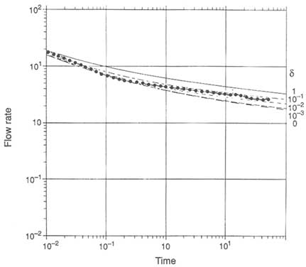
FIGURE 5.F6 Comparison of drawdown and flow for leakage into an infinite-sized rock with data from I2.1. From Wyss (1988).
and I3.1 (feature A). A weak but definite hydrological connection between I1.2 and I2.2 also was observed. Feature B in Figure 5.F1, which extends diagonally from the access tunnel to borehole 87.001, may partially explain this hydrological connection.
APPENDIX 5.G
THE FRACTURE ZONE PROJECT AT FINNSJÖN
The fracture zone project sponsored by SKB (Swedish Nuclear Fuel and Waste Management Co.) was run between the years 1984 and 1990 at the Finnsjön site, which is located in central Sweden about 140 km north of Stockholm. Its main goal was to characterize a major fracture zone in crystalline bedrock, especially the flow and transport properties of a fracture zone, the localization of potential pathways for groundwater flow, and transport of solutes essential for the safety assessment of a nuclear waste repository.
At the Finnsjön site, there are a number of gently dipping fracture zones (0° to 30° to the horizontal), which are common in such crystalline rock formations (Andersson, 1993). Geological identification and characterization of these fracture zones were accomplished through a broad range of geological, geophysical, geomechanical, geochemical, and hydrological investigations.
Through these investigations, a gently dipping fracture zone, zone 2, was defined in nine boreholes in an area of about 1,500 × 500 m in the northern part of the Finnsjön Rock Block at depths of 100 to 300 m. This zone was singled out for detailed flow studies aimed at understanding flow and transport in the zone and interactions with surrounding bedrock. Flow measurements on this zone included piezometric measurements, single-hole hydraulic tests at different scales, interference tests, groundwater flow measurements, and tracer tests, radially converging and dipole.
A number of hydrological modeling efforts were then undertaken. These efforts were carried out in conjunction with field experiments, so there was a close interaction between modeling and field measurements. In this interaction the modeling and field measurements mutually support each other; measurements can be used to test and improve the predictive ability of models, and models can be used to design and interpret field measurements. The overall sequence of this interaction was as follows:
-
model predictions of interference tests
-
interference tests
-
updated flow models based on interference tests
-
predictions of radially converging tracer tests
-
radially converging tracer tests
-
comparison of model predictions with radially converging tracer tests
-
prediction of dipole tracer test, and
-
comparison of model predictions with dipole tracer test.
The main conclusion regarding flow in zone 2 showed that the zone, which is about 100 m thick, is composed of two to five highly transmissive sections (T = 1 - 4 × 10⁻⁴ m2/s). These highly transmissive sections have widths of
about 0.5 m. Interference tests showed that the uppermost section was interconnected over distances of several hundred meters, and tracer experiments showed travel times differing by a factor of 10 between two observation boreholes at approximately the same distance from an injection borehole. Modeling efforts showed that zone 2 has a complicated structure where transport occurs in a few well-defined pathways and that this heterogeneity must be an important component in transport models.
REFERENCES
Abelin, H., L. Birgersson, J. Gidlund, and I. Neretnieks. 1991a. A large-scale flow and tracer experiment in granite 1. Experimental design and flow distribution. Water Resources Research, 27(12):3017–3117.
Abelin, H., L. Birgersson, L. Moreno, H. Widen, T. Agren, and I. Neretnieks. 1991b. A large-scale flow and tracer experiment in granite 2. Results and interpretation. Water Resources Research, 27(12):3019–3135.
Andersson, J. E., L. Ekman, R. Nordquist, and A. Winberg. 1991. Hydraulic testing and modeling of a low-angle fracture zone at Finnsjon, Sweden. Journal of Hydrology, 126:45–77.
Andersson, P. 1993. SKB Report 93-20, Swedish Nuclear Fuel and Waste Management Co., Stockholm.
Barker, J. A. 1988. A generalized radial flow model for hydraulic tests in fractured rock. Water Resources Research, 24(10):1796–1804.
Bear, J. 1979. Hydraulics of Groundwater. New York: McGraw-Hill.
Bennett, R. D., and R. F. Anderson. 1982. New pressure test for determining coefficient of permeability of rock masses. Technical Report GL-82-3, U.S. Army Engineer Waterways Experiment Station, Vicksburg, Miss., p. 61.
Black, J. H., and K. L. Kipp. 1981. Determination of hydrogeological parameters using sinusoidal pressure test: a theoretical appraisal. Water Resources Research, 17(3):686–692.
Bourdet, D., T. M. Whittle, A. A. Douglas, and Y. M. Pirard. 1983. A new set of type curves simplifies well test analysis. World Oil, 196:95–106.
Bourdet, D., J. A. Ayoub, and Y. M. Pirard. 1989. Use of pressure derivative in well test interpretation. SPE Formation Evaluation, 4(2):293–302.
Bredehoeft, J. D., and S. S. Papadopulos. 1980. A method for determining the hydraulic properties of tight formations. Water Resources Research, 16(1):233–238.
Bureau of Reclamation. 1985. Ground Water Manual. Denver: U.S. Department of the Interior, Bureau of Reclamation, p. 480.
Carrera, J., and S. P. Neuman. 1986. Estimation of aquifer parameters under transient and steady-state conditions: 2. Uniqueness, stability, and solution algorithm. Water Resources Research, 22(2):211–227.
Carrera, J., and J. Heredia. 1988. Inverse modeling of Chalk River block. NAGRA Technical Report 88-14, National Cooperative for the Disposal of Radioactive Waste (NAGRA), Baden, Switzerland, 117 pp.
Cooper, H. H., J. D. Bredehoeft, and I. S. Papadopulos. 1967. Response of a finite-diameter well to an instantaneous charge of water. Water Resources Research, 3(1):263–269.
Dagan, G. 1986. Statistical theory of groundwater flow and transport: Pore to laboratory, laboratory to formation, and formation to regional scale. Water Resources Research, 22(9):120S–134S.
Dagan, G., V. Cvetkovic, and A. Shapiro. 1992. A solute flux approach to transport in heterogeneous formations 1. The general framework. Water Resources Research, 28(5):1369–1376.
Da Prat, G., H. Cinco-Ley, and H. J. Ramey, Jr. 1981. Decline curve analysis using type curves for two-porosity systems. Society of Petroleum Engineers Journal, Society of Petroleum Engineers of AIME, pp. 354–362.
Dawson, K. J., and J. D. Istok. 1991. Aquifer Testing: Design and Analysis of Pumping and Slug Tests. Chelsea, Mich.: Lewis Publishers, p. 344.
Earlougher, R. C., Jr. 1977. Advances in Well Test Analysis. Dallas: Society of Petroleum Engineers of AIME, p. 264.
Gelhar, L. W. 1986. Stochastic subsurface hydrology from theory to applications. Water Resources Research, 22(9):135S–145S.
Garnier, J. M., N. Crampon, C. Preaux, G. Porel, and M. Vreulx. 1985. Tracage par 13-C, 2-H, I-et uranin dans la nappe de la craie senonienne en ecoulement radial convergent (Bethune, France). Journal of Hydrology, 78:379–392.
Hantush, M. S. 1967. Flow to wells in aquifers separated by a semipervious layer. Journal of Geophysical Research 72(6):1709–1720.
Hsieh, P. A., S. P. Neuman, G. K. Stíles, and E. S. Simpson. 1985. Field determination of the three-dimensional hydraulic conductivity tensor of anisotropic media 2. Methodology and application to fractured rocks. Water Resources Research, 21(11):1667–1676.
Johnson, C. R., R. A. Greenkorn, and E. G. Woods. 1966. Pulse testing: A new method for describing reservoir flow properties between wells. Journal of Petroleum Technology, Dec.:1599–1604.
Karasaki, K. 1990. A systematized drillstem test. Water Resources Research, 26(12):2913-2919.
Karasaki, K., J. C. S. Long, and P. A. Witherspoon. 1988. Analytical models of slug tests. Water Resources Research, 24(1):115–126.
Kucuk, F., and W. E. Brigham. 1979. Transient flow in elliptical systems. Society of Petroleum Engineers Journal, pp. 401–410.
LeBlanc, D. R., S. P. Garabedian, K. M. Hess, L. W. Gelhar, R. D. Quadri, K. G. Stollenwerk, and W. W. Wood. 1991. Large-scale natural gradient tracer test in sand and gravel, Cape Cod, Massachusetts 1. Experimental design and observed tracer movement. Water Resources Research, 27(5):895–910.
Long, J. C. S., J. S. Remer, C. R. Wilson, and P. A. Witherspoon. 1982. Porous media equivalents for networks of discontinuous fractures. Water Resources Research, 18(3):645–658.
Mackay, D. M., D. L. Freyberg, P. V. Roberts, and J. A. Cherry. 1986. A natural gradient experiment on solute transport in a sand aquifer 1. Approach and overview of tracer movement. Water Resources Research, 22(13):2017–2029.
Majer, E. L., L. R. Myer, J. E. Peterson, Jr., K. Karasaki, J. C. S. Long, S. J. Martel, P. Blumling, and S. Vomvoris. 1990. Joint seismic, hydrogeological, and geomechanical investigations of a fracture zone in the Grimsel Rock Laboratory. Report LBL-27913, NDC-14, Lawrence Berkeley Laboratory, Berkeley, Calif., 173 pp.
Maloszewski, P., and A. Zuber. 1985. On the theory of tracer experiments in fissured rocks with a porous matrix. Journal of Hydrology, 79:333–358.
Maloszewski, P., and A. Zuber. 1990. Mathematical modeling of tracer behavior in short-term experiments in fissured rocks. Water Resources Research, 26(7):1517–1528.
Maloszewski, P., and A. Zuber. 1992. On the calibration of mathematical models for the interpretation of tracer experiments in groundwater. Advances in Water Resources, 15:47–62.
Moench, A. F. 1984. Double-porosity models for a fissured groundwater reservoir with fracture skin. Water Resources Research, 20(7):831–846.
Moench, A. F. 1989. Convergent radial dispersion: A Laplace transform solution for aquifer tracer testing. Water Resources Research, 25(3):439–447.
Neuman, S. P., and P. A. Witherspoon. 1972. Field determination of the hydraulic properties of leaky multiple aquifer systems. Water Resources Research, 8(5):1284–1298.
Neuzil, C. E. 1982. On conducting the modified ''slug" test in tight formations. Water Resources Research, 18(2):439–441.
Novakowski, K. S., and P. A. Lapcevic. 1994. Field measurements of radial solute transport in fractured rock. Water Resources Research, 30(1):37–44.
Noy, D., J. Barker, J. Black, and D. Holmes. 1988. Crosshole investigations—Implementation and fractional dimension interpretation of sinusoidal tests. Stripa Project Technical Report 88-01, Swedish Nuclear Fuel and Waste Management Co., Stockholm, 62 pp.
Pickens, J.F., G.E. Grisak, J.D. Avis, D. W. Belanger, and M. Thury. 1987. Analysis and interpretation of borehole hydraulic tests in deep boreholes: principles, model development, and applications, Water Resources Research, 23(7):1341–1375.
Polek, J., K. Karasaki, J. Barker, and J. Long. 1989. Flow to wells in fractured rock with fractal structure. In Fractal Aspects of Materials, J. H. Kaufman, J. E. Martin, and P. W. Schmidt, eds. Materials Research Society.
Ramey, H. J., Jr., R. G. Agarwal, and I. Martin. 1975. Analysis of 'slug test' or DST flow period data. Journal of Canadian Petroleum Technology, July-Sept.:37–47.
Raven, K. G. 1986. Hydraulic characterization of a small groundwater flow system in fractured monzonitic gneiss. National Hydrology Research Institute Paper No. 30, Inland Waters Directorate Series No. 149, Environment Canada, Ottawa, Canada.
Raven, K. G., K. S. Novakowski, and P. A. Lapcevic. 1988. Interpretation of field tracer tests of a single fracture using a transient solute storage model. Water Resources Research, 24(12):2019–2032.
Sageev, A. 1986. Slug test analysis. Water Resources Research, 22(8):1323–1333.
Smith, L., C. W. Mase, and F. W. Schwartz. 1987. Estimation of fracture aperture using hydraulic and tracer tests. Pp. 453–463 in Rock Mechanics, Proceedings of the 28th U.S. Symposium, Tucson, Arizona, June 21–July 1. Farmer, I. W., J. J. K. Daemen, C. S. Desai, C. E. Glass, and S. P. Neuman, eds. Rotterdam: A. A. Balkema.
Streltsova, T. D. 1988. Well Testing in Heterogeneous Formations. New York: John Wiley & Sons, 413 pp.
Tsang, C. F., Y. W. Tsang, and F. V. Hale. 1991. Tracer transport in fractures: Analysis of field data based on a variable-aperture channel model. Water Resources Research, 27(12):3095–3106.
Tsang, Y. W., and C. F. Tsang. 1989. Flow channeling in a single fracture as a two-dimensional, strongly heterogeneous permeable medium. Water Resources Research, 25(9):2076–2080.
Welty, D., and L. W. Gelhar. 1989. Evaluation of longitudinal dispersivity from tracer test data. Report 320, Ralph M. Parsons Laboratory for Water Resources and Hydrodynamics, Massachusetts Institute of Technology, Cambridge.
Wyss, E., 1988. Kurzbericht zu den ersten hydrogelogischen Untersuchungen im Rahmen des Versuches FRI. SOLEXPERTS Field report to the Swiss National Cooperative for the Storage of Nuclear Waste (internal document).
Yeh, W. W. G. 1986. Review of parameter identification procedures in groundwater hydrology: The inverse problem. Water Resources Research, 22(2):95–108.
Zeigler, T. W. 1976. Determination of rock mass permeability. Technical Report S-76-2, U.S. Army Engineer Waterways Experiment Station, Vicksburg, Miss., 114 pp.


