
6
Field-Scale Flow and Transport Models
Previous chapters have addressed fracture geometry, physical and geomechanical properties of single fractures, fracture detection, and the interpretation of hydraulic and tracer tests. All of these elements must be integrated when developing a mathematical model to represent fluid flow and solute transport in fractured media. The focus of this chapter is mathematical models and the model-building process. The process of building a hydrogeological model crosses discipline boundaries, demanding the combined expertise of geologists, geophysicists, and hydrologists.
The hydraulic properties of rock masses are likely to be highly heterogeneous even within a single lithological unit if the rock is fractured. The main difficulty in modeling fluid flow in fractured rock is to describe this heterogeneity. Flow paths are controlled by the geometry of fractures and their open void spaces. Fracture conductance is dependent, in part, on the distribution of fracture fillings and the state of stress. Flow paths may be erratic and highly localized. Local measurements of geometric and hydraulic properties cannot easily be interpolated between measurement points. In contrast, granular porous media, although also heterogeneous, commonly exhibit smoothly varying flow fields that are amenable to treatment as equivalent continua. Model studies of fluid flow and solute transport in fractured media that do not address heterogeneity may be doomed to failure from the outset.
The formulation of a hydrogeological simulation model is an iterative process. It begins with the development of a conceptual model describing the main features of the system and proceeds through sequential steps of data collection and model synthesis to update and refine the approximations embodied in the
conceptual model. The conceptual model is a hypothesis describing the main features of the geology, hydrological setting, and site-specific relationships between geological structure and patterns of fluid flow. Mathematical modeling can be thought of as a process of hypothesis testing, leading to refinement of the conceptual model and its expression in the quantitative framework of a hydrogeological simulation model.
The relationship between the conceptual model, laboratory and field measurements, and the hydrogeological simulation model is illustrated in the flow chart in Figure 6.1. Simulation models are usually used as tools for enhancing understanding of flow systems as an aid in reaching management or design decisions. Three basic questions must be addressed before a model can be used as a site-specific design tool. First, does the conceptual model provide an adequate
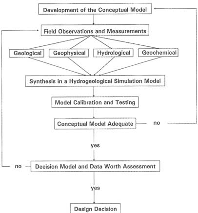
FIGURE 6.1 Flow chart identifying steps involved in the development of a hydrogeological simulation model for the purpose of reaching a management or design decision.
characterization of the hydrological system? If not, it should be revised and reevaluated. Second, how well does the model perform in comparison with competing models? Model results are nonunique. Consequently, field measurements may be successfully matched using fundamentally different conceptual and mathematical models. A model that successfully reproduces field measurements is not necessarily correct or validated. An important test of any model is to see how well it predicts behavior under changed hydrological conditions. Once the conceptual model is accepted, a third question must be asked: is the data base adequate to estimate the model parameters with sufficient reliability that the associated prediction uncertainties are acceptable in light of the intended application of the model in the decision process? If not, additional data collection is justified. In most instances this latter question is best addressed in an economic framework (Freeze et al., 1990).
The flow chart in Figure 6.1 is not unique to fractured geological media. It outlines the modeling process for any hydrogeological system. It is commonly the case, however, that these three questions are considerably more difficult to resolve when dealing with fractured media in comparison to problems involving fluid flow through granular porous media.
The purpose of this chapter is twofold: (1) to summarize recent views on the development of conceptual models of fluid flow and transport in fractured porous media and (2) to discuss and assess the state of the art in mathematical modeling and to identify research needs to advance modeling capabilities. The chapter focuses on general issues of model design. Mathematical formulations, numerical techniques, and specific computer codes are not included in the discussion. The chapter reviews the ways different types of simulation models incorporate the heterogeneity of a rock mass.
Much of the experience involving the simulation of fluid flow and solute transport in fracture systems has developed through the application of dual-porosity models in reservoir analyses. An extensive literature exists on the use of these models (e.g., Warren and Root, 1963; Kazemi, 1969; Duguid and Lee, 1977; Gilman and Kazemi, 1983; Huyakorn et al., 1983a,b; to name but a few). Although dual-porosity models are included in this discussion, greater emphasis is placed on more recent models that accommodate more complex fracture geometries than normally assumed in dual-porosity models. In addition, the discussion in this chapter is limited to fracture systems and model applications where it is not necessary to consider the effects of fracture deformation on fluid flow. This topic is addressed in more detail in Chapter 7.
DEVELOPMENT OF CONCEPTUAL AND MATHEMATICAL MODELS
Overview
Figure 6.1 highlights the central role of the conceptual model in the modeling process. When formulating a conceptual model to describe conductive fractures
and their permeabilities, three factors come into play: (1) the geology of the fractured rock, (2) the scale of interest, and (3) the purpose for which the model is being developed. These three factors determine the kinds of features that should be included in the conceptual model to capture the most important elements of the hydrogeology.
Geology of the Fractured Rock
A geological investigation seeks to identify and describe fracture pathways. These pathways are determined by material properties, geometry, stress, and geological history of the rock. There are two end members that describe the distribution of fracture pathways: (1) a system dominated by a few relatively major features in a relatively impermeable matrix, as commonly observed in massive crystalline rocks, and (2) a system dominated by a network of ubiquitous, highly interconnected fractures in a relatively permeable matrix, as might be found in an extensively jointed, layered rock with strata-bound fractures. Fracture systems exist at many levels between these two extremes in many different rock types. A geological investigation attempts to identify which features of a fracture system, if any, have the potential to dominate the hydrology.
Scale of Interest
A fracture system may be highly connected on a large scale, but it may be dominated by a few, relatively large features when viewed on a smaller scale. Classical thinking holds that the larger the scale of interest, the more appropriate it is to represent fractured rock in terms of large regions of uniform properties. The major problem then becomes one of estimating the large-scale properties from small-scale measurements. More recently, some workers have suggested that there are fracture features at all scales of interest. For these cases the traditional strategy of representing the rock as having large regions of uniform properties is less likely to be adequate. A series of new approaches are being developed to address fracture representation at large scales.
Purpose for Which the Model Is Being Developed
The level of detail required in the conceptual model depends on the purpose for which the model is being developed—for example, whether it will be used to predict fluid flow or solute transport. Experience suggests that, for average volumetric flow behavior, predictions can be made with a relatively coarse conceptual model provided data are available to calibrate the simulation model. Thus, a continuum approximation may be used to predict well yields with sufficient accuracy, even if a fracture network is poorly connected. For solute transport a considerably more refined conceptual model is needed to develop reliable predic-
tions of travel times or solute concentrations because of the sensitivity of these variables to the heterogeneity of fractured systems (Chapter 5). A more specific description of fracture flow paths may also be necessary to identify recharge areas for a well field located in a fractured medium.
The importance of identifying fracture pathways in contaminant transport problems can be visually demonstrated by observations from a laboratory model. Figure 6.2 illustrates the development of a solute plume in a fractured porous medium constructed from blocks of porous polyethylene. In this experiment a tracer was injected into a permeable matrix block for a period of 75 minutes, and its distribution was mapped. The pattern of spreading is complex and strongly dependent on the local structure and hydraulic properties of the network.
To this point, the conceptual model has been expressed in terms of a hypothesis describing the heterogeneity of the rock mass. In a more general sense, a conceptual model encompasses all of the assumptions that go into writing the mathematical equations that describe the flow system. Decisions are required about whether the problem at hand involves saturated or unsaturated flow, isothermal or nonisothermal conditions, single-phase or multiphase flow, and reactive or nonreactive solutes. Issues related to the development of conceptual models for these more complex processes are explored in the final section of this chapter.
The development of an appropriate conceptual model is the key process in understanding fluid flow in a fractured rock. Given a robust conceptual model, different mathematical formulations of the hydrogeological simulation model will likely give similar results. However, an inappropriate conceptual model can easily lead to predictions that are orders of magnitude in error.
Development of a Conceptual Model
The steps in building a conceptual model of the flow system include (1) identification of the most important features of a fracture system, (2) identification of the locations of the most important fractures in the rock mass, and (3) determination of whether and to what extent the identified structures conduct water. The important fractures are significantly conductive and connected to a network of other conductive fractures. All fractures are not of equal importance. Identification of preferred fluid pathways is crucial in the development of a conceptual model. So too is an understanding of the orientation of the fractures (or fracture sets) that contribute to flow, because these orientations provide insight into the anisotropic hydraulic properties of the rock mass.
Inferences about the relative importance of fractures can be made in a variety of ways. As described in Chapter 2, geological observation of fracture style is a powerful tool. Fractures have been studied in many locations and in many rock types, and several patterns have been identified (e.g., La Pointe and Hudson, 1985). For example, fractures may be evenly distributed in the rock mass or may occur in concentrated swarms or zones. There may be polygonal joints or
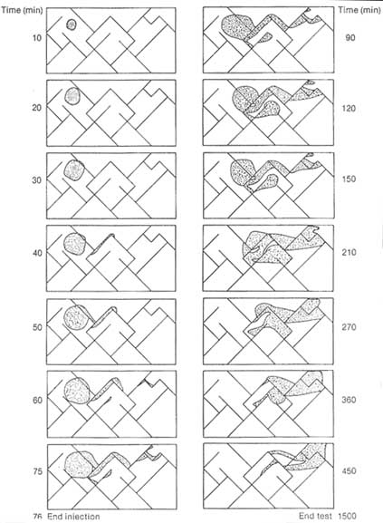
FIGURE 6.2 Laboratory experiment of tracer injection in a fractured porous medium. The model domain is 80 cm in length. Tracer was injected for 75 minutes and allowed to migrate under the influence of a uniform hydraulic gradient. The lines in the boxes represent the fracture networks. From Hull and Clemo (1987).
en-echelon features. Understandings gained through investigations of fracture style provide insights for predicting the character of fractures in unexposed parts of the rock mass.
Understanding the genesis of fractures can provide insights into the hydrological properties of the rock mass. For example, subvertical shear zones near Grimsel Pass in the Swiss Alps were studied in outcrop by Martel and Peterson (1991) and shown to have distinctly different fracture patterns depending on the orientation of the zone with respect to the fabric of the rock. Shear zones at an angle to the fabric (so-called K zones) tend to have parallel groups of fractures, whereas those parallel to the fabric (so-called S zones) have more braided, anastomosing fractures (Figure 6.3). The hydrological characteristics of these zones are likely to be quite different. K zones may have high vertical permeabilities in the vicinity of the fractures because they formed by extension; in contrast, S zones may be more uniformly, if anisotropically, permeable.
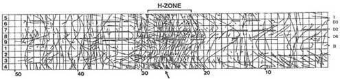
The Stripa mine in Sweden provides an example of another way to make inferences about fracture hydrology. A 50-m-long drift was excavated in the granitic rock mass, and every fracture with a trace longer than 20 cm was mapped (Figure 6.4). The rock appears to be ubiquitously fractured, with a concentration of fractures in the central 10 or 15 m of the drift (the H zone). Careful measurement has shown that essentially all the inflow comes from this zone; 80 percent of this inflow is from a single fracture (Olsson, 1992). Outside of this zone, the myriad other fractures are unimportant in contributing to the fluid influx. The zone itself does not behave as a homogeneous porous slab. It can be surmised that the flow systems in these zones are likely to be only partly connected. Fracture zones also dominate the hydrology at the Underground Research Laboratory in
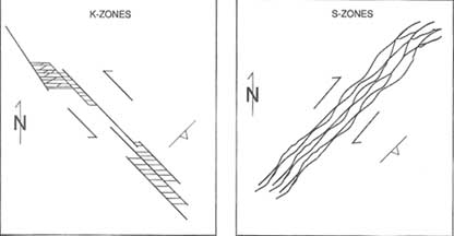
FIGURE 6.3 Schematic diagrams comparing the arrangement of fractures in K zones and S zones from the Grimsel Pass in the Swiss Alps. From Martel and Peterson (1990).
Canada (Davison et al., 1993) and at the Grimsel Rock Laboratory in Switzerland (Long et al., 1990).
The state of stress can be a controlling factor in determining which fractures or parts of fracture systems are important. An example is provided by a study in a fractured oil reservoir in the Ekofisk field in the North Sea (Teufel et al., 1991). Fractures with two distinct orientations were logged from boreholes; one of the sets was far more abundant than the other. Subsequent hydraulic testing showed that the direction of maximum permeability was aligned with the less abundant fracture set and that this direction was parallel to the maximum compressive stress. Apparently, fractures parallel to the maximum compressive stress tend to be open, whereas those perpendicular to this direction tend to be closed.
Once the flow-controlling fractures are identified, the next step is to define and locate them in the rock mass. Ideally, geophysical and geological data can be combined to determine the three-dimensional geometry of the major structures that might conduct water. Geological and geophysical investigations are clearly complementary. Geological investigations are well suited to identifying, locating, and characterizing exposed fractures and to determine how the fractures were formed; they are limited in their ability to determine how far to project known fractures into the rock and to detect unexposed fractures. Geophysical investigations can locate unexposed fractures, as discussed in Chapter 4, but are limited in their ability to uniquely determine the geometry of the detected fractures. Geological and geophysical methods do not generally yield quantitative information about the hydraulic and transport properties of fractures. They do provide information about the structure of the rock mass that can be used to organize hydrological investigations and interpretations.
There are two types of geological information available for integration with geophysical data: (1) geological maps of outcrops and (2) underground exposures and borehole data. The interpretation of borehole data has certain limitations. Individual borehole records typically do not allow the shapes and dimensions of fractures to be determined, nor do they provide information about fracture connectivity. In addition, the orientation of fracture zones, which can be determined from borehole measurements, can differ significantly from the orientation of individual fractures in the zone (e.g., the K zone in Figure 6.3). Methods of collecting and analyzing statistical data on fracture systems based on borehole observations are discussed in greater detail later in this chapter.
Finally, it must be determined if and how the identified fractures conduct water. There is probably no better way to see if a fracture conducts water than to pump water through it while monitoring the hydraulic response in the rock. A conceptual model of the fracture geometry provides a framework for designing this hydrological investigation. Instead of simply measuring injectivities at random, the tests can be focused on determining the hydrological properties of specific features. If the conceptual model includes a major feature, the well testing program can be designed to investigate the permeability of this feature. If there
are a number of features, the well tests can be designed to see if they are hydraulically connected. This diagnostic testing is described in Chapter 5. Geophysical tools described in Chapter 4, such as borehole flowmeters or borehole televiewers, also provide indications of the location of hydraulically conductive fractures. Under favorable circumstances, examination of the chemical composition of waters from different locations can provide an indication of water sources and whether or not the sources are mixing.
The result of this process is a model of those features of the fracture system that control the hydrology and some understanding of the nature of flow in the system. The process is by its very nature iterative. As data are collected and analyzed, the conceptual model is updated, and this may influence subsequent decisions on the types of data to be collected and on measurement techniques or locations. Revision of the conceptual model or selection of a competing model is driven by comparison of model predictions with new observations. An example of this process that emphasizes the role of geophysics is the conceptual modeling of the Site Characterization and Validation Experiment at the Stripa mine, which is discussed in Chapter 8.
Mathematical Models
Mathematical models fall into one of three broad classes: (1) equivalent continuum models, (2) discrete network simulation models, and (3) hybrid techniques. The models differ in their representation of the heterogeneity of the fractured medium. They may be cast in either a deterministic or stochastic framework. The scale at which heterogeneity is resolved in a continuum model can be quite variable, from the scale of individual packer tests in single boreholes to effective permeabilities averaged over large volumes of the rock mass. Discrete network models explicitly include populations of individual fracture features or equivalent fracture features in the model structure. They can represent the heterogeneity on a smaller scale than is normally considered in a continuum model. Some of the more recent innovations in mathematical simulation are best classified as hybrid techniques, which combine elements of both discrete network simulation and continuum approximations.
Table 6.1 presents a summary of the main classes of simulation models for fractured geological media. Included in this table are key parameters that distinguish the models. Also listed are references that illustrate recent applications of each modeling approach. The few references were chosen simply to point the direction toward the relevant literature; it is not meant to imply they are necessarily viewed as the ''best" papers on a given topic. Subsequent sections of this chapter explore these model types in greater detail. Additional coverage of some of these modeling concepts can be found in a recent text by Bear et al. (1993) and in another National Research Council (1990) report on groundwater models.
TABLE 6.1 Classification of Single-Phase Flow and Transport Models Based on the Representation of Heterogeneity in the Model Structure
|
Representation of Heterogeneity |
Key Parameters that Distinguish Models |
Recent Examples |
|
Equivalent Continuum Models |
||
|
Single porosity |
Effective permeability tensor |
Carrera et al. (1990) |
|
Effective porosity |
Davison (1985) |
|
|
|
Hsieh et al. (1985) |
|
|
Multiple continuum |
Network permeability and porosity |
Reeves et al. (1991) |
|
(double porosity, dual permeability, and multiple interacting continuum) |
Matrix permeability and porosity Matrix block geometry Nonequilibrium matrix/fracture interaction |
Pruess and Narasimhan (1988) |
|
Stochastic continuum |
Geostatistical parameters for log permeability: mean, variance, spatial correlation scale |
Neuman and Depner (1988) |
|
Discrete Network Models |
||
|
Network models with simple structures |
Network geometry statistics Fracture conductance distribution |
Herbert et al. (1991) |
|
Network models with significant matrix porosity |
Network geometry statistics Fracture conductance distribution Matrix porosity and permeability |
Sudicky and McLaren (1992) |
|
Network models incorporating spatial relationships between fractures |
Parameters controlling clustering of fractures, fracture growth, or fractal properties of networks |
Dershowitz et al. (1991a) Long and Billaux (1987) |
|
Equivalent discontinuum |
Equivalent conductors on a lattice |
Long et al. (1992b) |
|
Hybrid Models |
||
|
Continuum approximations based on discrete network analysis |
Network geometry statistics Fracture transmissivity distribution |
Cacas et al. (1990) Oda et al. (1987) |
|
Statistical continuum transport |
Network geometry statistics Fracture transmissivity distribution |
Smith et al. (1990) |
|
Fractal Models |
||
|
Equivalent discontinuum |
Fractal generator parameters |
Long et al. (1992) Chang and Yortsos (1990) |
In the process of calibrating a hydrogeological simulation model, assumptions and approximations on which the conceptual model is founded can be tested and refined. Competing models can be compared. The reality of hydrogeological simulation is that there may be a number of possible models with different combinations of geometry and media parameters that reproduce the observed response at a given point in the rock mass. Most flow and transport data from fractured rock sites are open to more or less equally successful interpretations by means of fundamentally different conceptual and mathematical models.
There is always a question about the uniqueness of the model. In selecting among different models that provide equally good matches to field measurements, two viewpoints exist. One favors a more parsimonious model, giving preference to models that are conceptually the simplest, that contain a smaller number of model parameters, and/or that contain the fewest number of quantities that are not readily measurable in the field on the same scale as they appear in the model. A second point of view favors models that are more "open ended" and look for a spectrum of structures, or distributions of permeability, that could explain the test data. Both approaches are being pursued in the research community. To evaluate these model results, there is a need for a more coordinated effort of cross-checking model predictions with field behavior, in a variety of fractured rock settings, on a variety of length scales.
Predictions of fluid flow and solute transport are normally subject to a considerable degree of uncertainty for several reasons. A fractured medium typically has a permeability structure that is highly variable and uncertain. Fluid flow and solute transport are sensitive to this heterogeneity. Changes in fluid pressure, through the effective stress, can modify the hydraulic properties of the fracture network. It is for these reasons that use of both the iterative approach and interdisciplinary investigations is critical to building confidence in model predictions. So, too, is the effort to quantify the magnitude of the uncertainty inherent in a model prediction.
In many instances, severe constraints on site characterization are encountered owing to limited project budgets, concerns about maintaining the integrity of a low-permeability rock mass, or concerns about cross-contamination of different horizons in the rock mass. There may be few boreholes in an area of several square kilometers. Funds may not be available for additional drilling or for detailed geophysical measurements. Consequently, it may not be possible to identify the positions or even the presence of connected pathways through a rock mass. Although geological models of the fracture system can be a great aid in these cases, the extent to which the hydrological model can be refined is limited. The unavoidable consequence of such constraints is the higher degree of uncertainty that is introduced into the hydrogeologic simulation model. Ideally, one would like to represent the fractured rock mass and the flow through it by models that accurately simulate the performance of each rock mass component. For the reasons just discussed, this is not possible, and all models are simplifications.
These simplifications may be introduced in the form of continuum models, in which the discontinuum character of the rock mass is neglected, or in the form of discontinuum models, which try to represent the discontinuities geometrically and mechanically. It is also possible to combine these modeling approaches. It is relevant to note that the difficulties in representing a fractured rock mass occur in many problems other than fracture flow, such as stability and deformability of the rock mass. Many of the models discussed in this chapter originate in these domains.
The simulation models listed in Table 6.1 are discussed in the following pages. The focus is on single-phase flow and transport in the saturated zone. The conceptual models that represent the heterogeneity of the rock mass are discussed with respect to the process of parameter estimation. Although their conceptual frameworks differ, all models are based on balance equations that express mass conservation in some representative volume of the rock mass. Examples of these models are described, and a few case studies are presented. The next section discusses the use of equivalent continuum models. Then alternative approaches that have been developed to address the complexities of flow peculiar to fracture systems are covered. More text is devoted to the discussion of discrete network and hybrid approaches because the hydrological community is generally less familiar with these concepts than with continuum models. One should not infer from the level of detail provided here that the committee always favors one approach over others. Models for more complex phenomena are discussed later in this chapter, including chemical processes, unsaturated flow, multiphase flow, and heat transfer. Fluid flow in deformable fractures is discussed in Chapter 7.
EQUIVALENT CONTINUUM SIMULATION MODELS
The Continuum Approximation
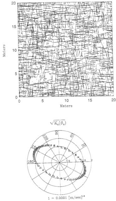
In a conventional equivalent continuum model, the heterogeneity of the fractured rock is modeled by using a limited number of regions, each with uniform properties. Individual fractures are not explicitly treated in the model, except when they exist on a scale large enough to be considered a separate hydrological unit (e.g., an areally extensive fracture zone). At the scale of interest, hydraulic properties of the rock mass are represented by coefficients, such as permeability and effective porosity, that express the volume-averaged behavior of many fractures. For example, Figure 6.5 shows a numerically generated fracture network. Flow through the network is calculated in many directions and is used to derive the equivalent permeability ellipse discussed below.
If the coefficients in the fluid flow and solute transport equations are viewed as being known with certainty, or if the most likely values of the variables are used, the model is deterministic. Conventional forms of the groundwater flow equation, which were developed originally for granular porous media, can then
be adopted. The use of continuum approximations in a deterministic framework has been the common practice.
If the coefficients are viewed as a spatially variable random field, characterized by a probability distribution, the model is stochastic. The magnitude of uncertainty in the input parameters depends on the natural variability of the medium, knowledge of which may be limited by the number and types of measurements available to map the heterogeneity.
Averaging volumes associated with a deterministic continuum approximation must be large enough to encompass a statistically representative sample of the open, connected fractures and their variable influences on flow and transport behavior. Effectively, this means that fluid flux and solute transport are not influenced to any significant degree by any individual fracture or its interconnections with other fractures that form the conducting network. The representation of a flow region using uniform flow properties is best applied to cases where the scale of the problem is large, the fractures are highly interconnected, and the interest is primarily on volumetric flow, such as in groundwater withdrawal for water supply. Rocks that have been subject to multiple and extensive deformations, and/or those with significant matrix permeabilities, are likely to be good candidates for equivalent continuum modeling. If, however, fracture density is low or many fractures are sealed by mineral precipitates, fracture connectivity may be low and continuum assumptions less likely to be adequate.
In the saturated zone, fractures usually provide the primary pathways for fluid flow and mass transfer. Matrix blocks between the conducting fractures can significantly increase the storage properties of the rock mass. Equivalent continuum models for fractured media are of two general types, single and dual porosity. In a single-porosity model all porosity is assumed to reside in the fractures; porosity in the matrix blocks between the conducting fractures is neglected. In a dual-porosity (fracture plus matrix) model the matrix blocks are assigned a value of porosity greater than zero. Single-porosity models represent hydrology in terms of a single continuum; dual-porosity models are based on two overlapping continuua.
For fluid flow problems involving steady-state conditions (i.e., no changes in fluid storage), single-porosity models are usually adopted. The fluid flux through the rock matrix is assumed to be negligible in comparison to that in the fracture network. For problems involving transient flow (i.e., a change in fluid storage), both single- and dual-porosity models have been used. As discussed later, the choice between a single- and a dual-porosity formulation relates to the manner in which the water released from storage in the fractures and matrix blocks is characterized. For problems involving solute transport in geological media with high matrix porosities or problems with long time scales, diffusion of mass between the fractures and the rock matrix (so-called matrix diffusion) can be an important process. Matrix diffusion is normally simulated by using a dual-porosity model.
This section reviews the approaches based on conventional applications of hydraulic test data to formulate estimates of the field-scale properties of the fractured medium. These applications include both deterministic and the more recent stochastic models. Continuum approaches that make use of discrete network models as a means of estimating field-scale continuum properties of the fractured medium are discussed later in this chapter, under "Hybrid Methods: Using Discrete Network Models in Building Continuum Approximations."
Single-Porosity Models Developed in a Deterministic Framework
Fluid Flow
Single-porosity models consider flow and transport only in the open, connected fractures of the rock mass. When using a numerical model, such as a finite-difference or finite-element model, a grid is superimposed on the flow domain and values of permeability are assigned to each grid block. Estimation of permeability involves a synthesis of laboratory and in situ measurements, model calibration, and model evaluation. The rock mass is normally represented by a limited number of hydrological units, each with homogeneous properties. These units may be isotropic or anisotropic. Because fractures typically occur in sets having preferred orientations, large-scale permeabilities may be anisotropic. An excellent example of a continuum approach is provided by Carrera et al. (1990), who modeled groundwater flow in a fractured gneiss at the Chalk River site in Ontario, Canada. They carried out an inverse simulation to identify a preferred model structure and to estimate the model parameters.
Hydraulic tests provide the most direct means of examining the validity of a porous medium approximation and for estimating values of the permeability tensor (Hsieh and Neuman, 1985; Hsieh et al., 1985). Single-borehole and crosshole hydraulic tests can provide this information (see Chapter 5), typically for volumes of rock having a characteristic length scale of tens of meters. If multiple nests of boreholes are tested, the question becomes one of how to use the values measured at this scale to estimate parameters representative of other scales of heterogeneity that are invariably present. Approaches to this issue represent one of the key research topics concerning the hydrology of fractured rocks. Geological and geomechanical models have an important role to play in providing a physical basis for extrapolating data beyond the measurement scale.
At the scale of hundreds of meters (subbasin scale), hydrogeological simulation models calibrated to estimates of recharge rates, water table positions, and/or potentiometric head data may provide the most reliable approach to estimate large-scale values for the conductance of the rock mass. Geochemical data, including isotopes and age dating of groundwater, also can be valuable for calibrating and testing hydrogeological simulation models. This general approach is probably most useful when predicting gross features of the flow system. As
emphasized in Figure 6.1, hydrogeological simulation is an iterative process. Model calibration can reveal the presence of fractures that may have been poorly sampled in the field, as happens, for example, with near-vertical fracture sets in an investigation program relying on vertical boreholes with no surface exposure. In this case, comparison of model predictions and field measurements may suggest horizontal anisotropy or a higher vertical permeability than was initially anticipated. An example of this case is discussed in Appendix 6.A.
For problems involving transient flow (e.g., a hydraulic disturbance caused by a pumping or injection well), a method to account for the fluid released from storage must be chosen. If fracture densities are high and matrix blocks are small, the fractured medium is sometimes treated as one effective continuum; that is, no distinction is made between fluid residing in the fractures or the matrix. The hydraulic diffusivity of the medium is a composite value reflecting the influence of both fractures and matrix blocks. The conventional equation describing transient groundwater flow in a porous medium is used in the simulation model (e.g., Freeze and Cherry, 1979).
Solute Transport
In a single-porosity transport model, the assumption is made that solute migrates only through the open, connected fractures in the rock mass. As indicated earlier, reliable prediction of solute transport in a fractured rock mass is considerably more difficult than the corresponding flow problem. Common practice, which is fraught with uncertainty, is to adopt the continuum approximations embodied in the conventional form of the advection dispersion equation. However, the scale at which a continuum approximation is valid may be at best difficult to determine, and at worst nonexistent. To define transport, the analyst must define the pathways through the flow system. This is equivalent, in a granular porous medium, to defining the subsurface configuration of streamtubes that connect the areas of groundwater recharge to the areas of discharge from the flow domain. It is because these pathways are so difficult to define in a fractured medium that there is considerable uncertainty in a transport simulation.
If an approximation based on porous medium equivalence is adopted, values are needed for the effective porosity and dispersive properties of the open fracture network. Estimation of effective porosity is key to predicting the average rate at which the solutes will move and to determining the mobility of solutes that react with the rock matrix. Mass will disperse as it encounters various pathways through the connected fractures. Invariably, an isotropic model for dispersion is chosen, whereby spreading is governed by three dispersivity coefficients that are independent of the angle of the hydraulic gradient. In fractured media, however, spreading is probably a highly anisotropic process; the character of spreading changes for different orientations of the hydraulic gradient. There are few experimental data of sufficient reliability to identify either a representative range of values for the
dispersive properties of fractured media or the character of the early time evolution of the dispersion process.
In principle, parameter estimates for effective porosity and dispersivity can be obtained from tracer tests. Although it is feasible to design and implement tracer tests to characterize the transport properties of fracture zones (see Chapter 5), transport properties of large fractured rock volumes are more difficult to characterize. Techniques for determining effective porosity are poorly developed. There are no general analytical expressions relating network geometry and the conductance of fractures to the three-dimensional dispersion tensor, analogous to expressions that have emerged in recent years for heterogeneous porous media. Furthermore, for fractured rock systems it is unclear how observations of tracer migration at small scales can be extrapolated to larger scales. Neuman (1990, 1994) has proposed a theoretical model that characterizes the scale dependence of dispersivity on average for all rock types (porous and fractured media). The approach provides an ensemble or, most likely, value at any given scale. If confirmed by further observations, this model will be useful in relating transport properties to the heterogeneity in permeability and to the information available to describe that heterogeneity.
Dual-Porosity Models
Fluid Flow
Dual-porosity models consider fluid flow and transport in both the connected fractures and the matrix blocks. For a rock mass with large porous matrix blocks between the conducting fractures, dual-porosity models have been used to account for the release of fluid from storage in the matrix blocks into the fracture network. The geometry of the fracture network is idealized to the extent that it can be represented by a small number of geometric parameters (e.g., the average dimension of a matrix block). Several examples are shown in Figure 6.6. The rock is characterized as two overlapping continuua, and both are treated as porous media. The key hydraulic properties are the effective permeability and porosity for the fracture network, the matrix porosity and permeability, and the storage coefficients for the fractures and matrix blocks. The equation expressing fluid flow through the fracture network contains source terms to account for flow from the matrix to adjacent fractures. A second set of equations describes fluid flow in the matrix blocks. Drainage into the fracture network depends on the geometry of the fracture-matrix interface and the hydraulic diffusivity of the matrix. Normally, a uniform geometry and block length are adopted for large regions of the flow domain. Some guidance in choosing a representative value for block length can be obtained from geological logs of fracture spacing.
An example that illustrates the application of a dual-porosity model using well logs to guide the selection of block size can be found in Moench (1984).
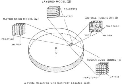
FIGURE 6.6 Idealization of a fractured reservoir adopted in a dual-porosity model. I, actual reservoir; II, sugar cube model; III, layered model; IV, match stick model. From Kazemi and Gilman (1993).
The case study deals with a well test at the Yucca Mountain site in Nevada. A borehole flow survey showed that there were five major zones of fluid entry over a vertical interval of 400 m (Figure 6.7). These zones were modeled as five horizontal zones of enhanced permeability, separated by slablike blocks of approximately 80 m thickness.
The match between the pumping test data and the type curves for the transient block-to-fracture flow model also is shown in Figure 6.7. The analysis gave values of hydraulic conductivity for the fracture system that were consistent with estimates obtained from single-borehole packer tests. Although values of hydraulic conductivity obtained for the blocks between the fracture zones were, to some degree, uncertain, estimated values from the dual-porosity model were in the range obtained by packer injection tests in intervals containing no major producing fractures. The values of hydraulic conductivity for the blocks were greater by two to five orders of magnitude than values measured on core samples, reflecting the presence of a connected fracture network in the blocks between the major fractures.
The primary advantage of dual-porosity flow models is that they provide a mechanism to account for the delay in the hydraulic response of the rock mass caused by fluid that is resident in less permeable matrix blocks. Dual-porosity
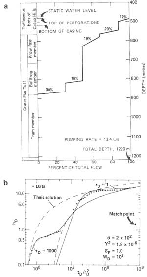
FIGURE 6.7 Interpretation of a pumping test in fractured rock at Yucca Mountain, Nevada, using a dual-porosity model. (a) Borehole flow survey showing percentage of total flow versus depth. (b) Match of the type curves for the dual-porosity model to the field data. The parameter rD is a dimensionless distance; other parameters given in the figure describe the hydraulic properties of the fractures and blocks. The parameters hD and tD are a dimensionless drawdown and dimensionless time, respectively. From Moench (1984).
models have been widely used in reservoir simulation (e.g., petroleum and geothermal reservoirs). The conceptual basis of dual porosity is appealing because of its simplicity. However, experience suggests that there are limits to the prediction capabilities of dual-porosity models. Two problems can be noted with these models: (1) they over regularize the geometry of the fracture network, and (2) good parameter estimates are difficult to obtain. Quantitative criteria to guide the choice between single- and dual-porosity formulations in site-specific applications are not easily defined. The choice of the appropriate conceptual model should be tested during its development (i.e., Figure 6.1).
Solute Transport
In cases where there is the potential for substantial diffusive transfer of mass into the rock matrix blocks, it is essential to incorporate this process into the mathematical structure of the simulation model. Concentration distributions can be greatly affected in comparison to a case in which mass is restricted to the open fracture network. This situation can arise, for example, in problems of regional-scale transport or in problems involving flow through geological units with high matrix porosities, as occurs in some sedimentary rocks and fractured clays. Transport can be facilitated by colloids because their large size limits the extent of matrix diffusion (e.g., McKay et al., 1993; Ibaraki, 1994). Two approaches are possible. One, discussed in a later section, models the fractures and matrix blocks as discrete features with specific geometric coordinates. The second, which uses a dual-porosity formulation, adopts a two-continuum representation of the fractures and matrix blocks, with matrix diffusion treated in a manner analogous to the fluid exchange between the fractures and the matrix.
A good example of the strengths and limitations of a dual-porosity transport simulation was published by Reeves et al. (1991). They investigated the potential for off-site migration of radionuclides through the Culebra dolomite at the Waste Isolation Pilot Project (WIPP) site in New Mexico. The Culebra dolomite is known to be fractured. The rock matrix also is porous, with an average porosity of 15 percent. Figure 6.8 shows their prediction of solute concentrations at the WIPP boundary, calculated for three different cases: (1) a single-porosity model, with flow only through the fractures; (2) a single-porosity model using an effective porosity equal to the sum of the matrix and fracture porosity; and (3) a dual-porosity model. The importance of mass diffusion into the matrix blocks is immediately apparent, as is the effect of dual-porosity structure.
Few quantitative data are available to characterize either the geometry or continuity of fractures in the Culebra dolomite. Observations from cores indicate that fracturing is not uniform even at the local scale. Reeves et al. (1991) adopted a uniform value of 2 m for the length of a matrix block. They also assumed that the fracture network could be represented as a single set of parallel fractures. Based on a travel time performance measure, they concluded that, in terms of
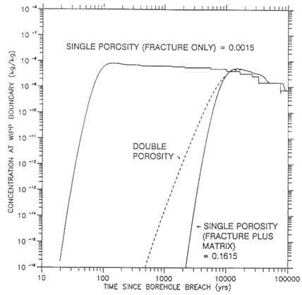
FIGURE 6.8 Example of a dual-porosity transport model. Predictions of solute concentrations for singleand dual-porosity representations of fractured rock at the WIPP site in New Mexico. From Reeves et al. (1991).
the need for additional characterization, data on the matrix block length and matrix porosity ranked first and second, respectively, for a set of seven model parameters that described solute transport in the Culebra dolomite.
Stochastic Continuum Models
The stochastic representation of fluid flow and solute transport in heterogeneous porous media has led in recent years to a powerful new set of tools for hydrogeological analysis. These tools have also been applied to fractured geological media (e.g., Neuman, 1987). The basis of stochastic models is the representation of hydraulic properties in terms of probability models that describe the medium as a random field. In adopting a stochastic approach, the modeler
acknowledges that a complete and accurate simulation of fluid flow, or the movement of a contaminant plume in a fractured rock mass, is not a realistic goal. Instead, it is argued that predictions of plume geometry that are expressed in terms of the spatial moments of the plume (i.e., the mean position and spread of the mass about the mean position), or statements cast in probabilistic terms to describe mass breakthrough at a downstream boundary, provide a better framework for implementing and interpreting predictive simulations. The stochastic framework can also provide estimates of prediction errors in concentration and travel time. Stochastic continuum concepts have been proposed for single-porosity models, and there is no difficulty, in principle, in extending the approach to a dual-porosity formulation.
It is normally assumed that the fractured medium is heterogeneous, but the statistical parameters that describe the heterogeneity are uniform in the region of interest (statistical homogeneity). If this assumption is appropriate, the probability model characterizing the fractured medium is reduced to a form expressed in terms of a mean, variance, and three-dimensional correlation structure for each variable of interest (e.g., hydraulic conductivity and porosity). The correlation structure is a measure of the degree of spatial continuity of the hydraulic conductivity values. The many tools developed for geostatistical analysis of heterogeneous media come into play here (e.g., Isaaks and Srivastava, 1989). Estimates of hydraulic conductivity from single-hole packer tests provide the point values for statistical characterization of the heterogeneity. Figure 6.9a illustrates log hydraulic conductivity profiles obtained from straddle packer tests in several boreholes at the Oracle site in Arizona (Jones et al., 1985). The semivariogram characterizing the spatial continuity in log hydraulic conductivity is plotted in Figure 6.9b. The fractured granite is represented by a continuous but spatially varying set of hydraulic properties. Figure 6.9c is one possible representation of the hydraulic conductivity variations along a cross section connecting four boreholes. This representation preserves the values measured at the borehole locations, yielding a so-called conditional stochastic model.
Once the hydraulic conductivities have been estimated, stochastic flow theory provides equations to estimate the effective conductivity ellipse for an anisotropic porous medium (e.g., Gelhar and Axness, 1983; Dagan, 1987). These equations can also be used to estimate a set of field-scale dispersion coefficients. This approach has been illustrated for a fractured rock system by Neuman et al. (1985) and Neuman and Depner (1988). The stochastic equations also permit estimates to be made of the magnitude of the uncertainties in flow and transport predictions. As an alternative to estimating parameter values in a governing stochastic equation, multiple realizations of the hydraulic properties of the rock mass can be generated from the probability model (e.g., Figure 6.9) and used in a Monte Carlo simulation to estimate probability distributions of output variables, such as volumetric flows or groundwater travel times.
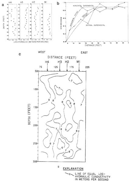
FIGURE 6.9 Geostatistical characterization of hydraulic conductivity at the Oracle site in Arizona. (a) Log hydraulic conductivity profiles from straddle packer tests in four boreholes. (b) Anisotropic semivariogram of log hydraulic conductivity. (c) Geostatistical representation of hydraulic conductivity variations from four boreholes (M1, H2, H3, H4). The plot shows a single realization generated from the conditional stochastic model. From Jones et al. (1985).
The important practical advantage of this stochastic approach is that it works directly with field measurements of hydraulic conductivity, rather than a suite of parameters characterizing network geometry. Its validity depends on the suitability of approximations embodied in the representation of the fractured rock mass as a heterogenous porous medium with a statistically homogeneous structure and in the suitability of mathematical simplifications that underlie stochastic transport theory.
Assessment of Continuum Modeling
The strength of the continuum approach lies in its simplicity; it reduces the geometric complexity of flow patterns in a fractured rock mass to a mathematical form that is straightforward to implement. For most applications that are encountered in practice, some type of continuum approach remains the preferred alternative. The two greatest limitations of deterministic continuum models of the kind most widely used today are (1) the scale at which the continuum approximation is justified can be difficult to quantify and in fact may not be justified at the scale of interest or, for that matter, at any scale and (2) the process of spatial averaging restricts model predictions to scales greater than or equal to that of the representative elemental volume (REV). The concept of the REV may be irrelevant to most field measurements, especially in fractured rock (Beveye and Sposito, 1984, 1985; Neuman, 1987, 1990). Most small-scale field measurements do not correspond to REVs. If these measurements represent a statistically homogeneous field, then under special circumstances, such as uniform mean flow in an unbounded media, an REV can be defined on a scale that exceeds many times the spatial correlation scale of the measured data (and many more times the scale of the actual local measurement) (Long et al., 1982; Neuman and Orr, 1993). Seldom can the corresponding REV scale permeability be determined directly by field tests and almost never so in low-permeability fractured rocks. In most circumstances, and especially in multiscale media of the kind fracture rocks are thought to be, an REV can never be defined. If the concept of an equivalent continuum is not applicable in reality then there may be a broad class of hydrogeological problems that are not amenable to analysis with conventional continuum models. This concern is particularly relevant in the case of solute transport.
It is common in a fracture system to find well test responses that are not normally viewed as indicative of continuum behavior. For example, for a pumping well with two observation wells, the farther observation well may respond more quickly than the nearer one. This type of response is due to the nature of fracture interconnections. While such behavior can be reproduced in a continuum model by adopting a heterogeneous hydraulic conductivity distribution (i.e., a local-scale representation of the spatial variability in hydraulic conductivity), the appropriate model structure will end up looking much like a discrete fracture model.
Stochastic continuum models, which represent the fractured rock mass as a continuous random field, represent one approach to dealing with issues of scale. The scale at which the heterogeneity is represented in the model can be tailored to the scale at which measurements of permeability are made in the field. Probabilistic predictions of fluid flow and solute transport can then be made at a larger scale.
A number of important issues have yet to be resolved in applying continuum approximations. There is the basic issue of applicability and robustness of assumptions that underlie a continuum representation. There is the issue of how to identify the scale at which the continuum approximation is valid, if there is one. There is a need to develop an understanding of what field observations, including but not limited to hydraulic interference testing, may be helpful in indicating the scale of continuum behavior. A description of the dominant fluid pathways in a fractured rock is critical in a transport simulation. Methods for implementing this information in the framework of a continuum model require further investigation, especially in the case of sparsely fractured rock masses.
DISCRETE NETWORK SIMULATION MODELS
Why Consider Discrete Network Models?
Fractured masses are composed of blocks separated by discontinuities, and therefore discontinuum models may be an attractive approach to representing these systems. Discontinuities occur at a variety of scales; they have different geometries and flow properties, and these properties may vary with location and direction. Discontinuum models must account for these complexities. In particular, the fact that discontinuities are not persistent (i.e., they are bounded by intact rock) is most significant because the characteristics of intact rock and of the discontinuity differ substantially. (This is not only so for fluid flow in a rock mass but also for rock mass stability and deformability.) The knowledge of individual fracture characteristics in situ is limited, and the persistence of fractures is not known. This so-called persistence problem can only be solved through the use of stochastic models and probabilistic approaches incorporated into these models.
Discrete network models are predicated on the assumption that fluid flow behavior can be predicted from knowledge of the fracture geometry and data on the transmissivity of individual fractures. The guiding principle is that spatial statistics associated with a fracture network, including fracture transmissivity, can be measured, and these statistics can be used to generate realizations of fracture networks with the same spatial properties. The fractures in these realizations become the conductive elements in a fracture network flow or transport model (e.g., Hudson and La Pointe, 1980; Long et al., 1982; Dershowitz, 1984; Endo et al., 1984; Robinson, 1984; Smith and Schwartz, 1984). Application of
network models to field sites requires the measurement of fracture geometry to construct models that reproduce the observed statistics of the geometry of the fracture network. This method involves choosing a stochastic rule for locating fractures and determining their orientation, extent, and conductivity. Various issues involved in collecting and analyzing statistical data on fracture networks are reviewed later in this section, followed by the outline of a number of models that have been proposed to represent the statistical characteristics of fracture networks.
Discrete network models are closely linked with concepts of stochastic simulation. Network geometry is characterized by statistical descriptions of fracture orientation, location, areal extent, and transmissivity for each of the fracture sets in the rock mass. From this statistical model it is possible to generate multiple realizations of a fracture network and to solve for fluid flow through each network. Each realization is one possible representation of the fracture network in the rock mass from which the geometric properties were mapped. For example, Figure 6.10 shows three different fracture networks, each of which is one realization from stochastic models with differing fracture densities (expressed as a scan line density, i.e., the average number of fractures per meter encountered along horizontal and vertical sample lines).
For each realization a large-order system of equations is solved to determine the distribution of hydraulic head at all points in the fracture network. This is accomplished by modeling flow in each fracture and ensuring conservation of fluid mass at fracture intersections. By averaging the flow behavior for a large number of realizations of the same stochastic model in a Monte Carlo simulation, inferences can be made about the expected behavior of the system and the variability about the mean. The behavior of interest may be fluid flux across the fracture network or, in the case of a contaminant transport problem, the travel time of solutes from a recharge boundary to the outflow boundary. This property is illustrated in Figure 6.10, where the mean and standard deviations in breakthrough time at the downstream boundary are given for the three different fracture densities. In this case the standard deviation can be interpreted as a measure of the uncertainty in predicting the time at which solutes first arrive at the downstream boundary. Similar statistics on the arrival time of mass at the downstream boundary could have been developed by using the stochastic continuum approach if, instead of characterizing the network geometry, the rock mass had been represented as a continuous random field of local-scale permeability values. This figure clearly demonstrates the strong dependence of travel time statistics on the geometric properties of the fracture network.
By conditioning the model on the location of known fractures or measured values of fluid flux, it is possible to quantify the extent to which uncertainty is reduced with the availability of specific types of field data. Anderson and Thunvik (1986) generated multiple realizations of a fracture network; each network preserved the locations of fractures that would have been mapped in a set of hypotheti-
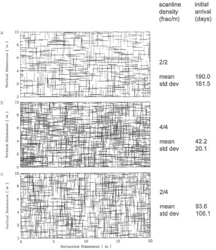
FIGURE 6.10 Examples of single realizations for three fracture systems with differing fracture densities (measured as scanline densities; see text). Numbers on the right are the mean and standard deviations of travel times for solutes that enter the left side of the systems through a single fracture and travel downstream to the right side of the systems. Modified from Smith and Schwartz (1993).
cal boreholes. As expected, they found that adding more boreholes (and thus adding information on the location of fractures as mapped on the borehole walls) decreased the uncertainty in a transport prediction. However, other factors such as fracture length, fracture line density, and the spatial correlation of aperture along a fracture exerted a strong influence on the value of the geometrical data
obtained from borehole logging. Knowledge of the bulk permeability of the fracture network led to a greater reduction in uncertainty than the collection of additional geometrical data on fracture location. This response occurred because knowing fracture location along a borehole does not provide information about fracture extent. The information is not sufficient to determine interconnectivity and therefore permeability (Long and Witherspoon, 1985). Conditioning on the bulk permeability provided a stronger constraint on estimates of the rate of advective mass transfer than did geometric data on fracture location without additional information on fracture connectivity, which cannot be obtained from borehole fracture intersections.
To apply discrete network models in a field setting, it is essential to have the capability for three-dimensional simulation. In these models, fractures are represented as disk-shaped or polygonal features, rather than line segments. The degree to which higher-transmissivity regions on one fracture plane connect with those on other fractures will determine the connectivity of the network, fluid pathways, and transport patterns. By modeling flow in each fracture and ensuring conservation of fluid mass at fracture intersections, a large-order system of equations is solved to determine the distribution of hydraulic head at all points in the fracture network. A number of three-dimensional flow models are described in the literature (e.g., Long et al., 1985; Shapiro and Anderson, 1985; Elsworth, 1986; Dverstrop and Anderson, 1989). Examples of the application of different three-dimensional network flow models are the studies by Dershowitz et al. (1991a), Long et al. (1992b), and Herbert et al. (1991) of the Stripa Site Characterization and Validation Experiment. Also, some work has been reported on three-dimensional network models for solute transport (Smith et al., 1985; Cacas et al., 1990; Dershowitz et al., 1991a, b; Herbert and Lanyon, 1992; Nordqvist et al., 1992; Segan and Karasaki, 1993a).
Three-dimensional network models are of three general types: (1) semi-analytical models (e.g., Long et al., 1985); (2) equivalent one-dimensional pipes arranged in three-dimensional space (e.g., Segan and Karasaki, 1993); and (3) discretized fracture planes, where a two-dimensional numerical grid is constructed in each fracture plane (e.g., Smith et al., 1985; Dershowitz et al., 1991a; Herbert and Lanyon, 1992). A network of planar fractures may require 105 to 106 nodes to adequately resolve the flow field, even for a relatively sparse fracture network. When it is necessary to generate multiple realizations of the network for analysis, computational requirements are very demanding.
One-dimensional pipe models have been adopted in an attempt to reduce the computational requirements associated with a fully three-dimensional representation. The fracture network is first generated in a three-dimensional framework and then is collapsed to a system of one-dimensional pipes to solve for fluid flow. Flow in each fracture plane is reduced to a single representative pipe centered in the middle of the fracture plane (Cacas et al., 1990) or to an arbitrary number of pipes (Segan and Karasaki, 1993). A one-to-one correspondence
between pipe properties and the actual three-dimensional geometry governing flow is theoretically possible. However, the actual geometry governing flow is rarely, if ever, known. The model parameters are probably best viewed as calibration variables rather than physically based properties of the medium.
Geological Issues in the Statistical Representation of Fracture Networks
Some geological settings may be more amenable to statistical analysis of fracture patterns than others. The statistical method will work best if (1) the fracture pattern is uniform in a statistical sense (statistical homogeneity); (2) it is possible to obtain a sample that is statistically representative; (3) the spatial distribution of fractures is not too complex, that is, it can be described by a simple rather than a compound stochastic process; and (4) the fractures used to determine fracture statistics actually do conduct fluid. Favorable conditions for discrete network modeling might best be met, for example, in some jointed rocks. These factors are similar to the conditions suited to the application of continuum models. Consequently, discrete models may also provide a method for obtaining the parameters used in continuum models, as discussed later.
Strata-bound joints that have relatively regular patterns in a given strata have been observed in bedded volcanics and sedimentary rocks such as bedded limestones (Pollard and Aydin, 1988). Joint patterns amenable to statistical analysis also have been observed in massive rocks (Segall and Pollard, 1989). Joints commonly occur in subparallel sets with variable spacing. Figure 2.30 shows some common joint system patterns. These patterns provide the basis for many of the conceptual models described below. The existence of common joint geometries with recognizable patterns has been one of the primary motivations for the statistical approach.
The nature of joint intersections is an important attribute of joint systems. Some examples are shown in Figure 2.30. If joints intersect other joints, a hydraulic connection can be formed between them. If one set terminates near another without actually intersecting, there may be no hydraulic communication.
Joint systems can exhibit complexities that affect statistical modeling of network geometry. Joint frequency may be spatially variable. Spacing can be a function of depth, lithology, or bed thickness. Joint clusters or zones also occur and may be difficult to include in a statistical model. Joints are commonly formed episodically and have segments corresponding to each episode, each with varying properties. Extensive folding and faulting of jointed rock may be responsible for the development of large dominant flow structures that are not well represented in a statistical sense. Multiple deformations can lead to preferential fracturing along preexisting planes of weakness, resulting in a style of fracturing that is very heterogeneous and complex.
It is important to recognize that, owing to a variety of geological processes, large parts of the observable fracture system may be uninvolved in fluid circula-
tion. This issue points to a basic concern for the discrete fracture approach because it uses the observable fracture geometry to predict flow and transport behavior. A significant proportion of fractures may be nonconductive, because they are either closed or sealed by mineral precipitates. A model based on fracture occurrence without accounting for fractures that are nonconductive will vastly overestimate interconnectivity. This lack of interconnection is the main reason that discrete network models are chosen over equivalent continuum models, but it is also the reason that homogeneous network models may fail to capture the distribution of hydraulic conductors and consequently fail to reproduce the hydraulic behavior of the fracture network.
Evidence of hydrologically inactive fractures has been found at numerous sites. For example, at the Fanay-Augeres mine in France, thousands of fractures were mapped in tunnel walls and in boreholes from the tunnel. Models created with fracture size, orientation, and location statistics for this tunnel resulted in highly interconnected fracture networks (Long and Billaux, 1987; Billaux et al., 1989; Cacas et al., 1990). However, none of these models were able to reproduce the fundamental observation that there is no hydraulic communication between some of the boreholes. Another example is the Stripa mine, discussed earlier, where 80 percent of the water flowing into a drift was carried by one fracture, even though many of the observed fractures have the same orientation and should have roughly the same state of stress acting on them. These measurements suggested a high degree of interconnection in the observed fracture network (Herbert et al., 1991). However, out of thousands of fractures intersecting the drift, only a few conducted water.
Stochastic Models of Fracture Networks
The representation of discontinue and solution of the persistence problem only became possible with the introduction of stochastic models for representing network geometry. As will be seen below, the first stochastic fracture models had only a few stochastic characteristics; the remainder were spatially invariable. Most important, fractures (discontinuities) were unbounded, thus not providing a solution to the persistence problem. The introduction of bounded fractures came with the introduction of two models: the Baecher disk model and the Veneziano polygonal model. Most subsequent fracture network models for rock mass flow, rock mass stability, and rock mass deformation were based on these models. Although these models represented a major advance, the assumed independence of their geometric characteristics made representation of typical fracture properties such as clustering impossible. Spatial dependence in stochastic models was introduced through a variety of statistical and quasi-mechanistic concepts (Long and Billaux, 1987; Lee et al., 1990; Martel et al., 1991) and through fractal representation (Barton and Larsen, 1985). The increasing complexity of the
models brings them closer to reality but makes the inference procedures by which the field data can be transferred into the model increasingly difficult.
Two classes of stochastic models can be used to describe fracture systems. One is based on the assumption that the occurrence of one fracture has no influence on the positioning of any subsequent fracture that is generated to form the network. Fracture centers are located by using a uniform probability distribution. These models are discussed here and are reviewed in more complete detail by Dershowitz and Einstein (1988). The second class of models allows for a spatial dependence between the positioning of neighboring fractures, and it leads to networks with recognizable, scale-dependent characteristics. This latter class of models is discussed later in this chapter. Both model classes have rules for specifying fracture characteristics, including (1) the location of fractures in space; (2) the shape of fractures; (3) the extent of fractures, including truncations against other fractures; (4) the orientation of fractures; (5) the conductive properties of fractures; and (6) in some cases the conductive properties of fracture intersections.
Orthogonal Models and Their Extensions
The simplest fracture model is the orthogonal model that is based on three sets of unbounded orthogonal fractures (Figure 6.11). In two dimensions this corresponds to the network shown in Figure 2.30a. This model was characterized
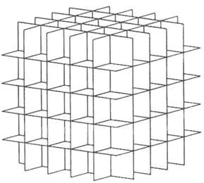
FIGURE 6.11 Three-dimensional orthogonal fracture model. From Dershowitz and Einstein (1988).
by Irmay (1955) and Childs (1957), among others. A series of models can be created as modifications of this basic structure by allowing the orientation, extent, location, and conductivity of the fractures to vary (Snow, 1965). For example, the networks in Figure 2.30 c–f can be considered two-dimensional modifications of the orthogonal model.
Poisson Plane Models
Probably the most important stochastic process used to define fracture system geometry is the Poisson process. This random process is controlled by only one parameter, a density parameter, that specifies the average density of objects in space—that is, the average number of objects (points, lines, or planes) per unit line length, unit area, or unit volume. Priest and Hudson (1976) were the first to recognize the similarity between the geometry of rock fracture systems and the attributes of Poisson processes. In particular, the distances along a line sample between objects of a Poisson process are distributed according to a negative exponential distribution. This distribution is commonly observed for fracture spacing along a scanline. The simple Poisson plane fracture model of Priest and Hudson was based on the assumption of unbounded fractures. In their model, fractures were located randomly by having each fracture pass through a point in space that is determined by a Poisson process. The orientation of the plane was then determined independently, according to an appropriate probability distribution.
More complex models are defined with bounded fractures. These models are of two types: (1) those that define fracture shape and size distribution a priori and (2) those that define a process that, in turn, defines fracture shapes and sizes. For the first type of model, fractures are usually assumed to be rectangles or ellipses. They can have any size distribution and are placed in space centered on Poisson points and oriented randomly according to any distribution specified (see Figure 6.12). Such models have been developed by Baecher et al. (1977), Barton (1978), and Robinson (1984). The Baecher model has been used in rock mechanics applications by Einstein et al. (1980, 1983) and Warburton (1980a,b) and for fracture flow modeling by Long et al. (1982, 1985) and Dershowitz (1984). The Robinson model has been used by Herbert et al. (1991) at the Stripa mine. Geier et al. (1989) proposed an extension to the Baecher model to account for the probability of fractures in one set terminating at the intersection with another set. It is also possible to use the Poisson process to create a polygonal grid of fracture elements (a pattern similar to Figure 2.30g; see Khaleel, 1989).
The second type of model defines a stochastic process to determine fracture shape and size. The usual process is to start with the unbounded Poisson planes and superimpose on them a series of Poisson lines. The lines can be created independently, as in Figure 6.13 (Veneziano, 1978), or by the lines of intersection between the unbounded Poisson planes, as in Figure 6.14 (Dershowitz, 1984).
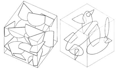
FIGURE 6.12 Baecher disk model of a fracture system. From Dershowitz and Einstein (1988).
The lines divide the planes into polygonal areas, each of which is then assigned some probability of being an open fracture. It is very easy to construct networks with coplanar fractures with these models. Veneziano (1978) demonstrated that this type of model leads to an exponential distribution of fracture trace lengths, which contrasts with the lognormal distribution found in the Baecher model. The Veneziano model has been applied to slope stability problems by Einstein et al. (1983) and to the hydrology of fractured rock masses by Rouleau (1984). Both of these applications utilized the Veneziano model in a two-dimensional trace plane only. The geometry of the Veneziano model is quite complex in three dimensions.
Estimation of Model Parameters for Statistical Models of Fracture Networks
To build a fracture network model, field data must be collected to estimate the parameters of the stochastic model used to represent the network geometry. The following data are normally required:
-
Fracture location as observed in boreholes or along scanlines in either surface outcrop or subsurface excavations.
-
Fracture orientation from borehole logs, core, surface outcrop, or subsurface excavations. The orientation of fractures that intersect planes may have to be estimated from apparent orientation, that is, the orientation of the trace of the fracture plane.
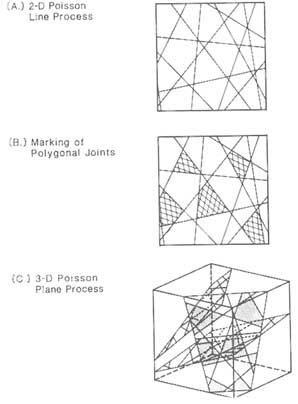
FIGURE 6.13 Veneziano polygonal model of a fracture system. From Dershowitz and Einstein (1988).
-
Fracture trace length in outcrop or underground excavations.
-
The percentage of fractures that terminate against other fractures as a function of orientation, as obtained from outcrop or underground excavation.
-
Estimates of the transmissivity of individual fractures from hydraulic tests.
There are two approaches to using this data to parameterize the models described above. In the first approach the parameters of the model are calculated directly from the fracture statistics. This method works best for the simplest models, primarily those based on simple Poisson processes. A good example of this approach was the work of Herbert et al. (1991) at Stripa. As more of the spatial relationships between fractures are accounted for, it is harder to calculate the parameters directly. In these cases an inverse approach becomes more attractive. In the inverse approach a set of parameters is proposed for a given conceptual
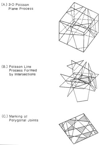
FIGURE 6.14 Dershowitz polygonal model of a fracture system. From Dershowitz and Einstein (1988).
model and used to generate the geometry of a fracture network. Then a series of simulated networks is sampled in a manner congruent to that used in the field: simulated boreholes or surfaces are used to collect fracture spacing, orientation, and trace length. The simulated data are compared to the real data, and adjustments are made to the model parameters to improve the fit to the observed data. In effect, this is model calibration. Dershowitz et al. (1991a) provide a good example of this approach.
All fracture data collection procedures are affected by uncertainties introduced by the sampling procedure (errors, biases, statistical fluctuations), which,
combined with the spatial uncertainty discussed throughout this chapter, model uncertainties, boundary condition uncertainties, and omissions, affect the representation of geology and engineering performance predictions (for a complete discussion of uncertainties in engineering geology, see Einstein et al., 1980). Of particular interest in the context of this section are the uncertainties caused by errors and biases. In the following discussion on data collection for stochastic model representation, typical biases that must be considered will be mentioned. These are only examples and they are far from complete. For a more comprehensive treatment of sampling biases and errors, including possible corrections, see Einstein et al. (1979) and Baecher (1972).
Fracture Density
To build a Poisson model, the fracture density per unit volume must be known. The advantage of the Poisson distribution is that analytical relationships exist between densities that can be measured and those that are needed to generate a network. For example, given the density of fracture intersections along a line (i.e., fracture frequency) and the fracture size and orientation distributions, it is possible to calculate the expected number of fractures per unit volume (volumetric fracture density). A simple example is for fractures with mean area, A, and a distribution of orientations, f (![]() ), where
), where ![]() is the angle between the fracture poles and the sample line (e.g., a borehole). The fracture pole is the unit vector perpendicular to the fracture plane. The relationship between volumetric density (number of fractures per unit volume, Nv) and linear density (fracture frequency, NL) is
is the angle between the fracture poles and the sample line (e.g., a borehole). The fracture pole is the unit vector perpendicular to the fracture plane. The relationship between volumetric density (number of fractures per unit volume, Nv) and linear density (fracture frequency, NL) is
where <cos ![]() > is the mean orientation of the fracture set (Terzaghi, 1965). This equation shows that the probability of encountering a fracture in a borehole, NL, is proportional to the fracture size and the number of fractures per unit volume, Nv. This probability is higher for fractures perpendicular, cos
> is the mean orientation of the fracture set (Terzaghi, 1965). This equation shows that the probability of encountering a fracture in a borehole, NL, is proportional to the fracture size and the number of fractures per unit volume, Nv. This probability is higher for fractures perpendicular, cos ![]() = 1, to the borehole than for fractures parallel to it, cos
= 1, to the borehole than for fractures parallel to it, cos ![]() = 0. Consequently, if the sample lines are parallel to the fractures, it may be difficult to get a good estimate of fracture density.
= 0. Consequently, if the sample lines are parallel to the fractures, it may be difficult to get a good estimate of fracture density.
Fracture Orientation
Obtaining the orientation distribution is conceptually simple but practically difficult. Errors in the construction of orientation data sets are common because the analysis is three-dimensional and there are many potential sources of error. After correction, the orientation in space of each fracture encountered in the sample is measured. The pole of each fracture is normally plotted on a stereographic projection, either a Wolff net or a Schmidt net. Then clusters can be identified and used to group fractures into sets. For each set the orientations can
be fitted to a distributional form such as a spherical normal (or Fischer) distribution (Mardia, 1972), or the sample distribution can be used itself. There is some sentiment that identification of fracture sets by an ''eyeball" fit may be as effective as the more sophisticated analytical methods.
It is necessary to account for possible sampling biases. In the case of the orientation distribution, this bias arises from the difficulty in determining the orientation distribution for fracture sets parallel to the sampling line or plane. The Terzaghi (1965) approach to correcting for orientation bias is to divide the density of fractures in a similarly oriented group by <cos ![]() >, where
>, where ![]() is the angle between the sampling line or plane and the poles of the fractures for that group, thereby increasing the frequency of fractures parallel to the sample line. This approach has the underlying assumption that the sampling of fractures nearly parallel to the borehole is representative. It is not possible to know whether the absence of fractures parallel to the borehole is real or is due to sampling bias. An alternative proposed by Martel (1992) and Martel and Peterson (1993) involves comparison of the sampled orientations with orientation distributions obtained by sampling a series of synthetic distributions in the same manner that field data were taken. In this way one can determine if the sampling scheme is sensitive to the possible choices of orientation distribution.
is the angle between the sampling line or plane and the poles of the fractures for that group, thereby increasing the frequency of fractures parallel to the sample line. This approach has the underlying assumption that the sampling of fractures nearly parallel to the borehole is representative. It is not possible to know whether the absence of fractures parallel to the borehole is real or is due to sampling bias. An alternative proposed by Martel (1992) and Martel and Peterson (1993) involves comparison of the sampled orientations with orientation distributions obtained by sampling a series of synthetic distributions in the same manner that field data were taken. In this way one can determine if the sampling scheme is sensitive to the possible choices of orientation distribution.
Fracture orientations obtained from outcrop or underground excavations can be measured directly if the fracture surfaces are exposed. Otherwise, only apparent orientations can be measured, that is, the orientation of the fracture trace. Orientation data can also be obtained from boreholes by using the logs described in Chapter 4 or from core, although there can be difficulties in getting reliable data. Cores tend to twist on extraction, causing orientation errors. Pieces may be missing or broken, making it difficult to orient sections of the core. Borehole imaging logs (Chapter 4) can be used where there is missing core. More fundamentally, the orientation of the fracture where the core was taken may not be representative of the average orientation of the fracture. On the practical side, there is probably no other effort in the analysis of fracture statistics that deserves a good-quality assurance program as much as the data collection and reduction process for fracture orientation.
Fracture Size
From available exposures, the distribution of fracture size is obtained from the orientation data and fracture trace data. Rarely, if ever, can the actual areal extent of a fracture be observed directly. The trace length sample must first be corrected for bias, as discussed below. Then the corrected trace length distribution can be used to predict the distribution for fracture area. The relationship between the trace length distribution and the size distribution depends on fracture shape. Normally, it is necessary to make an assumption about the shape of the fracture (e.g., disk-shaped) and then estimate the size distribution from the sample data.
When mapping in adits, it is important to distinguish between fractures caused by blasting and those that reflect in situ conditions. It is also important to characterize the types of fracture intersections. Fractures may either cross or one may terminate against the other. Termination can be quantified simply by noting the percentage of fractures of a given set that terminate against other fractures.
There are four biases affecting the estimation of fracture size: length bias, orientation bias, truncation bias, and censoring. Small fractures will be underrepresented, as there is a lower probability of intersecting smaller fractures than larger fractures (length bias). Fractures parallel to the sampling plane will also be underrepresented (orientation bias). Fractures shorter than a predetermined length are usually not mapped (truncation bias). A censoring bias is introduced because the sample area is finite, and the fracture traces may not be completely visible (Baecher et al., 1977). Censoring bias is most important for longer fractures, which are generally the more conductive fractures. With respect to censoring bias, fracture traces can be divided into three groups: (1) traces with both endpoints visible, (2) traces with one endpoint visible, and (3) traces with no endpoints visible. The trace length distribution of the first group can be determined. These fractures have a maximum length determined by the dimensions of the sample area. For the second group a distribution of minimum lengths can be found. For the third group all that is known is that the fracture traces are larger than the sample dimensions. Some analytical solutions to the censoring problem have been obtained by assuming a distributional form for the trace lengths (Long and Billaux, 1987; Einstein et al., 1979, vol. IV). Similarly, if a distributional form is assumed for the fracture areas, one can use the corrected trace length distribution to estimate the parameters of the area distribution (Long and Billaux, 1987). Dershowitz et al. (1991a) have developed an automated procedure for generating fractures of a given size distribution and sampling the system the same way the field data were sampled. The prospective area distributions can be easily modified until a good (but necessarily unique) match to the field data is found. If only borehole measurements are available, problems associated with obtaining estimates of fracture size can be severe.
Transmissivity of Individual Fractures
In applying a discrete network model, the characterization of transmissivity values is likely to be a dominant source of uncertainty in a flow or transport simulation. It was once thought that the hydraulic conductivity of each fracture could be obtained from a physical measurement of aperture and application of the cubic law (Iwai, 1976). As explained in Chapter 3, complications of roughness, filling, and contact area indicate that fracture transmissivity should be measured directly. Such in situ measurements have been attempted through packer tests from boreholes. An interval, as small as practical, is isolated in a borehole, and a well test is carried out. The transmissivity calculated from the test is then
attributed to the fractures intersecting the borehole interval. A number of assumptions must be made in order to obtain the distribution of fracture transmissivities from these borehole tests. Usually it is not possible to isolate single fractures. Consequently, one must decide how to distribute the observed transmissivity among the fractures that intersect the borehole interval. Further, in calculating the transmissivity, it is normal to assume that the fractures are infinite in extent and perpendicular to the borehole. Fracture intersections, branching, and terminations are not accounted for. Any correlation between fracture transmissivity and length is very difficult to determine, but such correlation significantly increases network permeability (Shimo and Long, 1987).
Local estimates of transmissivity from a number of well tests provide an initial estimate of the statistical distribution of transmissivity for individual fractures. However, these estimates are significantly affected by lack of information about the number, relative conductance, orientation, and extent of fractures intersecting the test zone and the intersection of the tested fractures with other fractures. Thus, it is usually not possible to obtain good estimates of fracture transmissivity distributions, and it is inevitable that some kind of model calibration will be required to refine the estimates of fracture transmissivity.
Calibration of a discrete network model can involve estimates for hundreds or thousands of variables (e.g., an effective transmissivity value for each fracture in the network). An even greater number of variables is introduced if the inversion seeks estimates of transmissivity for fracture segments between intersections, relaxing the assumption that each fracture has a single transmissivity. Inevitably, there will be no unique set of transmissivity values that explain the observational data. An alternative calibration strategy is to simply refine estimates of the mean and variance of the transmissivity distribution, by matching the observed variability in transmissivity to that predicted by the model.
Applications of Discrete Network Models in Media with Significant Matrix Porosity
Discrete network models are necessarily more complex in cases where (1) the permeability of the rock mass in which the fracture network is embedded is a significant fraction of the network permeability or (2) the porosity of the rock matrix is high or the time scale of interest is long enough that diffusive mass transfer becomes a factor in determining large-scale solute transport patterns. Several methods have been developed to model flow and solute transport in geological units containing a network of fractures embedded in a porous matrix. The fracture network is modeled explicitly, unlike a conventional dual-porosity model. McKay et al. (1993) have applied an analytical model describing advective/diffusive transport in evenly spaced, parallel fractures to model tracer tests at an experimental site in a fractured clay till. The principal difficulties in solving these problems numerically are the different time scales involved for transport
along the fractures and in the matrix and the need for a fine grid resolution to represent sharp concentration gradients at the fracture-matrix interface. Using a Laplace transform technique in conjunction with a finite-element model, Sudicky and McLaren (1992) have overcome these problems. Figure 6.15 provides an example showing a calculation of the concentration distribution in both the fracture network and the matrix blocks in a medium where matrix porosity is 30 percent. The concentration distribution bears little resemblance to that which would be observed in an unfractured aquitard. Similarly, matrix diffusion is effective in slowing down the rate of advance of contaminants through the aquitard, in comparison to a case where mass transport is limited to the fracture network. Dershowitz and Miller (1995) describe an implementation of a discrete fracture model in which matrix diffusion is simulated using a probabilistic particle tracking technique. Okusu et al. (1989) created a mesh generator that can discretize the matrix for any two-dimensional fracture network. Given the mesh, a variety of flow and transport models can be invoked.
Another possibility for solving this problem is to treat the fracture flow explicitly and the matrix flow semianalytically. The flow into or out of the matrix can be determined through the use of a proximity function that describes the cross-sectional area of the matrix block as a function of distance from the fracture (Pruess and Karasaki, 1982; Figure 6.16). The fracture network (Figure 6.16a) is divided into connected elements and dead-ends plus isolated fractures (Figure 6.16b). The matrix area is divided into regions that are equidistant from connected fractures (Figure 6.16c). It is then possible to construct a "proximity function" that gives the cross-sectional area of matrix as a function of proximity to a fracture containing fluid flow. This function can be used in a double-porosity model to describe fracture-matrix interactions in a statistical sense.
Assessment of Discrete Network Models
There are two views concerning the utility of discrete network models. One view is that they are primarily a tool for concept evaluation or model-based process studies (e.g., Long and Witherspoon, 1985; Smith and Schwartz, 1984). Studies of this type have proven useful in examining requirements for characterization of a fracture network as an equivalent porous medium, studying the scale dependence of the dispersion process, examining how network geometry influences spreading patterns, and evaluating issues related to the reliability of data on fracture position and orientation.
The second view is that discrete network models are practical tools for site-specific simulations (e.g., Dershowitz et al., 1991a; Herbert and Lanyon, 1992). The advantage of a discrete fracture simulation is that volume-averaging approximations are avoided at the scale of the fracture network. In cases where an equivalent continuum cannot be defined, discontinuum network simulation is a viable alternative.
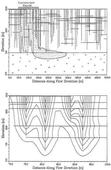
FIGURE 6.15 Prediction of solute distribution using a discrete network model in a medium where matrix diffusion is important. A fractured low-permeability aquitard overlies a permeable aquifer (lower unit). The fracture network is shown as straight lines; the contours of contaminant concentration appear as curved lines. The upper plot shows the plume at t = 200 years. Only the outer contour with a normalized concentration of 0.01 is shown. The lower plot is a detailed view of a part of the plume. The outer contour is a normalized concentration of 0.1; the contour interval is 0.1. From Sudicky and McLaren (1992).
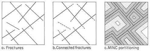
FIGURE 6.16 Illustration of the construction of a proximity function for an arbitrary two-dimensional fracture distribution. (a) Fracture network. (b) Connected fractures in the network are indicated by solid lines; extensions of the fractures that are not conductive are shown by dotted lines. (c) Division of the matrix area into regions (indicated by different patterns) that are equidistant from the connected fractures. These regions are used to calculate the proximity function. From Pruess and Karasaki (1982).
To be useful as a simulation tool, discrete network models must incorporate information concerning the dominating fracture features and their positions in three-dimensional space. These capabilities exist. The disadvantages of discrete network simulation are threefold: (1) the method requires statistical information that can be difficult to obtain, (2) it is difficult to separate the conductive fracture geometry from the nonconductive fracture geometry, and (3) the models can be complex and computationally intensive for realistic fracture densities.
These models have been useful in problems of near-field simulation over length scales of 50 to 100 m. Application to larger-scale problems will require modifications such as treating fracture zones as a single fracture in the model and screening of fractures to eliminate the less transmissive ones.
Although theoretical studies using fracture network models have provided valuable insights on how to determine equivalent continuum properties of fractured rock, it is extremely difficult to actually determine continuum properties in the field. The magnitude of permeability estimates is critically dependent on the values assigned to fracture transmissivity. Mechanical measurements of fracture aperture are of little value in this regard, as they do not capture the influence of the internal geometry of the fracture plane on the hydraulic resistance to flow. The observed fracture pattern may not be strongly related to the equivalent permeability if, for example, a significant percentage of the fractures are sealed by mineral precipitates or are closed owing to the stress regime. Billaux et al. (1989) and Cacas et al. (1990) describe how such approaches were applied in an adit at Fanay-Augeres in France and led to hydrological models that are highly overconnected compared to the real system. Calibration data of some kind (e.g., an observed fluid flux) are needed to apply these methods. Whether it be for continuum models or discrete network models, too few prediction studies have been checked against subsequent behavior.
Perhaps the most often heard comment about discontinuum models is that they are not practical. Consequently, researchers have tried to show that this style of model better captures the hydraulic system behavior of a fracture system in order to justify the apparent extra expense. The problem with discontinuum models, as for any model of fracture flow, is that it is extremely difficult to construct a field test that can prove that a model is valid. (This has led some researchers to develop pragmatic definitions of the word validate, shaped by what they expect to be able to accomplish rather than what would ideally constitute validation.) Most field tests designed to test and compare models have concluded that a variety of models, including discontinuum models, can reproduce the observed behavior of the system (see, e.g., Olsson, 1992). However, to focus on these projects as validation exercises is to miss the major accomplishment of such work, which is to increase understanding of the hydrology of the media involved. The particular style of modeling is much less important than whether the model includes the features that are dominating the behavior of the system. In fact, during the lifetime of the Stripa Site Characterization and Validation
Project, four teams were developing models of flow and transport for the site. (See Olsson, 1992, for an entree to this literature.) Although these models started from very different approaches, they became more similar with time as more was learned about the site and what features at the site were hydrologically important. The hydrologically dominant fracture zones had to be explicitly entered into all the models, continuum or discontinuum, in order to match the observed behavior. Whether or not the discontinuum codes were more or less efficient than the continuum codes was simply a matter of how they were applied, that is, whether they included and discretized every observable fracture or whether major zones of fractures became one large fracture in the model. These exercises have shown that discontinuum models can be used effectively and may be very efficient at reproducing the lack of connectivity in a fracture network.
HYBRID METHODS: USING DISCRETE NETWORK MODELS IN BUILDING CONTINUUM APPROXIMATIONS
Fluid Flow
Because it is difficult or impossible to measure large-scale permeability directly, it would be extremely useful to be able to estimate such values by taking some kind of average of the local-scale measurements. In the case of fracture systems, discontinuum models can provide a framework for attempting such an analysis. If it is possible to build a discontinuum model based on field data, it may be possible to obtain an estimate of large-scale continuum properties. However, all the difficulties in parameterizing discontinuum models that are described in the previous section apply as well to this endeavor. The use of discontinuum models to study how fracture systems will behave on a large scale has taken two approaches. One approach is to perform numerical flow experiments using fracture network models. The second approach reaches estimates of continuum behavior by looking at the networks as a percolation problem.
Estimation of Continuum Properties from Fracture Network Analysis
Several equations have been developed to estimate the permeability tensor by combining hydraulic data on fracture transmissivity with data on fracture frequency and orientation obtained from geological surveys. One of the first of these equations was developed by Snow (1965). Snow measured the frequency and orientation of fractures encountered in a borehole or along a scanline and combined these data with estimates of hydraulic aperture from packer tests. He assumed that all the fractures were infinite in length and could be modeled as parallel plates. An equivalent permeability tensor was calculated from the orientation and hydraulic aperture of each fracture by simply adding the components from each fracture. Oda (1985) and Oda et al. (1987) developed an analytical
formulation of the permeability tensor that applies to fractures of finite length The basic assumption underlying this formulation is that fracture density is high enough that nearly all the fractures contribute to the effective permeability. Thus, this formula applies to essentially the same cases as Snow's. From an engineering perspective, these equations are the best available to relate fracture geometry to a larger-scale hydraulic conductance. They are limited by the difficulty of obtaining representative estimates of hydraulic apertures and of distinguishing between the apparent and conductive fracture geometry. Most importantly, these methods do not account for the effect of fracture connectivity. This approach was applied to predict the hydraulic properties of fractured granite around a ventilation drift at the Stripa mine. Given estimates of an average hydraulic aperture from in situ tests, estimates of effective permeability were within one order of magnitude of measured values.
Long et al. (1982), Robinson (1984), Dershowitz (1984), and Hudson and LaPointe (1980), among others, have extended the approach of estimating continuum properties from a fracture network analysis by developing models of fluid flow in fracture networks. The fracture networks are specified by giving the location, orientation, extent, and hydraulic aperture of each fracture. The fractures are assembled into a network, and fluid flow through the network is calculated with standard numerical techniques.
The calculated behavior of these networks can be compared to that of a continuum in a variety of ways. Long et al. (1982) suggested calculating a series of directional permeabilities, K(![]() ) measurements. It is possible to plot 1/K(
) measurements. It is possible to plot 1/K(![]() ) as a function of the gradient direction,
) as a function of the gradient direction, ![]() , on a polar plot. This plot will be a perfect ellipse if the medium is behaving as an equivalent continuum. For a less than perfect ellipse, a regression analysis can be used to fit these data to the permeability tensor (Figure 6.17). The regression error is then a measure of how well the medium can be represented as an equivalent continuum. The idea is similar to that proposed by Hsieh et al. (1985) for analysis of interference data, as described in Chapter 5. Any of the network models described in the previous section could be used in this manner to estimate a permeability tensor.
, on a polar plot. This plot will be a perfect ellipse if the medium is behaving as an equivalent continuum. For a less than perfect ellipse, a regression analysis can be used to fit these data to the permeability tensor (Figure 6.17). The regression error is then a measure of how well the medium can be represented as an equivalent continuum. The idea is similar to that proposed by Hsieh et al. (1985) for analysis of interference data, as described in Chapter 5. Any of the network models described in the previous section could be used in this manner to estimate a permeability tensor.
Cacas et al. (1990) provide an interesting demonstration of an approach for estimating the large-scale permeability of fractured rock using statistical data on network geometry in combination with a model calibration using small-scale hydraulic and tracer tests. The analysis was based on data from an adit in a highly fractured granite at Fanay-Augeres, France. The injection test data consisted of 180 flow measurements, using a packer spacing of 2.5 m, obtained in 10 boreholes. Total inflow to the adit also was recorded. Data were also available from 10 tracer injection experiments, four of which yielded breakthrough curves adequate for use in model assessment. They proceeded as follows: (1) A stochastic, three-dimensional, discrete network model was constructed and used to generate a number of realizations of the fracture network. To solve for the distribution of flow in each realization, the network was reduced to a set of one-dimensional
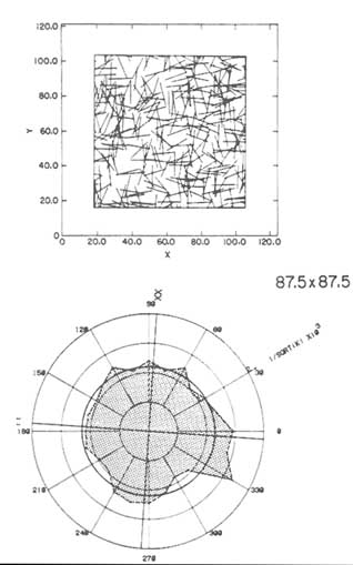
FIGURE 6.17 Example of a polar plot of the inverse of the directional hydraulic conductivity for the fracture network shown in the upper plot. From Long (1983a).
"pipes" connecting each fracture intersection to the center of the fractures. (2) The conductance of the pipes was interpreted as a stochastic parameter and was characterized by the mean and variance of its distribution. The mean and variance of the pipe conductance were taken to be the calibration parameters. Values were estimated so that the mean and variance of the flow rates observed in the set of synthetic realizations matched the observed mean and spread in the histogram of injection flow rates. (3) The calibrated flow model was then used to generate 17 "intermediate-scale" realizations, and a hydraulic conductivity ellipse was
estimated for each. (4) These intermediate-scale values were averaged, using equations developed for heterogeneous porous media, to estimate a large-scale hydraulic conductivity for the rock mass surrounding the adit.
The flow model was tested by using a set of hydraulic head measurements from around the adit, together with measured inflow rates to the adit, to estimate a single hydraulic conductivity value, applicable at a scale of 100 m. The value obtained fell within the range of the global hydraulic conductivity estimated using the stochastic discrete network model. Tracer tests were then used to test the estimate of the variance of the pipe conductance. Using the calibrated flow model, 20 realizations of each tracer injection experiment were generated. A single transport parameter, related to fracture volume, was adjusted so that the peak arrival times in each set of realizations were consistent with the variation in the time of peak arrival observed in the tracer tests. To provide another test of the flow model, a comparison was made with the calibrated transport model to see if the model reproduced the observed variability in breakthrough durations. (The breakthrough duration is a function of the variance in the pipe conductance.) The distribution of the breakthrough duration times was consistent with the values observed in the tracer tests, without any additional calibration of the variance of the pipe conductances.
The study by Cacas et al. (1990) showed how field data obtained at one scale can be analyzed in a stochastic framework to provide larger-scale estimates of the hydraulic conductivity of an equivalent porous medium. In adopting a stochastic framework, they attempted to reproduce the structure of the fracture network only in a statistical sense and not in terms of identifying specific locations around the adit where the connectivity may be higher or lower than average. It is important to note, however, that this model (and the more complex model of Billaux et al., 1989, described later) failed to accurately represent the lack of hydraulic interconnection at Fanay-Augeres because it was based on apparent fracture geometry rather than conductive fracture geometry. The Fanay-Augeres experience illustrates dramatically that it is not enough to look at fracture statistics, or fracture pattern for that matter, to be able to understand the hydrology of a fracture system. It is critical that data be collected that show how the system is hydraulically interconnected. This statement implies that one must create a hydraulic signal at various points in the system and monitor whether that signal is received at other points in the system. In other words, it is critical to do interference testing and tracer testing to see if the system is interconnected. Mapping the fractures and single-well hydraulic tests simply cannot provide this critical information.
Estimation of Continuum Properties Based on Percolation Theory
As described in Appendix 6.B, percolation theory is the study of random networks of conductors. In some cases it is possible to map a discrete network
model into a simple lattice percolation model. This map, together with results from percolation theory, can be used to derive analytical expressions for the permeability of the network model (Hestir and Long, 1990).
A simple lattice percolation model is constructed by creating a lattice of conductors and randomly turning some of them off, as shown in Figures 6.18a and b. The parameter that describes this stochastic model is p, the probability that a given conductor is left on. Analytical expressions for approximating permeability in such lattices have been given in the physics literature for some time (for example, Kirkpatrick et al., 1983). These expressions give permeability in terms of p when p is near the critical probability, pc. The critical probability pc corresponds to the value of p below which there are only finite clusters of connected conductors (no percolation) and above which there are infinite clusters of connected conductors (percolation).
One way to develop expressions for permeability as a function of the stochastic network parameters is to relate a discrete network model to a simple percolation model. Several authors have developed relationships between permeability and the average number of intersections per fracture, ς, where ς is a measure of the connectivity (see Appendix 6.C on connectivity). This method has been implemented for two-dimensional discrete networks of random line segments (e.g., Figure 6.18c) by Robinson (1984), Hestir and Long (1990), and Berkowitz and Balberg (1993). In the work of Robinson and Hestir and Long, for example, a way was found to determine the effective values of p and z as a function of ς. Hestir and Long show that a good fit to numerical simulations of fracture network permeability can be found by using the following expression for p derived by finding the average length of a line in the lattice model as a function of p and the average length of a line in the random line model as a function of ς and then equating the two averages to get an expression of p in terms of ς:
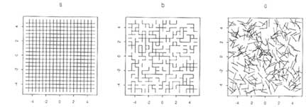
FIGURE 6.18 Percolation networks. (a) Square lattice with all conductors present. (b) Same lattice with a fraction 1 — p of the original conductors removed. (c) Random percolation network of uniform-length line segments.
Then, using percolation theory (see Appendix 6.B), an expression for permeability near the critical limit can be developed:
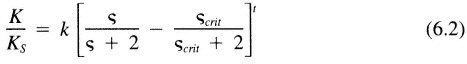
where Ks is a normalization constant corresponding to the case where ς is infinite, k is a constant, ςcrit is the value of connectivity where percolation begins, and t is a universal exponent with a value of about 1.2. This method depends on being able to calculate the average line length in the random model. This is possible for simple Poisson models but may become extremely difficult for more complex stochastic systems. This limitation prevents direct application of the method in many cases, but the general concept of connectivity and percolation behavior is expected to hold in any random network. Thus, these theories do provide an intellectual platform for understanding the development of permeability.
Solute Transport
As indicated earlier, one of the key difficulties in the formulation of a field-scale model to represent solute transport in fractured rock is estimation of the parameters that characterize the dispersive properties of the rock mass. Model studies have been used to examine equivalent porosity in much the same way that models have been used to examine equivalent permeability. Endo et al. (1984) created a mechanical transport model by tracing streamtubes through a two-dimensional network model assuming no mixing in the fracture intersections. Just as in Figure 6.17, flow and transport were examined in a variety of directions through the models. For each direction the ratio of fluid flux to mean velocity was calculated (i.e., equivalent hydraulic porosity). Endo found that even systems that behaved like equivalent porous media for flux had values of hydraulic equivalent porosity that varied with the direction of flow, as shown in Figure 6.19. In a similar manner, both tortuosity and dispersivity were found to vary significantly with flow direction. In most practical situations, with limited project budgets and short time horizons, tracer tests are not a viable option for formulating parameter estimates. One approach, based on stochastic theories of transport in heterogeneous porous media, was outlined earlier. The present section outlines a second approach, based on the development of transport characteristics at the continuum scale by simulating transport at a smaller scale using a discrete network model.
Schwartz and Smith (1988) proposed a statistical continuum model to simulate anisotropic dispersion in a network of finite-length, randomly located fractures of variable aperture. Particle tracking is at the core of the method. Solute transport is modeled by first collecting statistics on particle motion in a subdomain model using a discrete network simulation and then using these statistics in a continuum
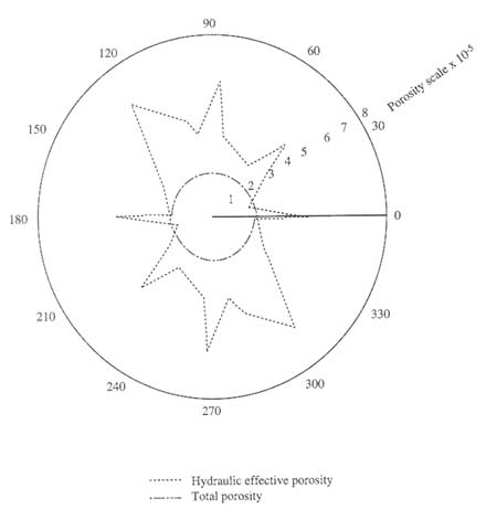
FIGURE 6.19 Polar plots of total porosity and hydraulic effective porosity for discontinuous system with mean fracture length of 50 m and linearly correlated apertures. From Endo (1984).
model to simulate transport at a larger scale. Particle tracking also is used in the continuum model, so there is never a need to assign numerical values to a dispersion tensor. This, in fact, is the primary advantage of the technique. In essence, the particles are ''educated" in the discrete model. Then, in the continuum model, they are able to mimic the effects of the interaction between network geometry and conductance, the orientation of the hydraulic gradient, and the resulting spreading patterns.
The discrete network model is a small piece of the much larger domain for which field-scale simulation is required, but it is intended to be representative. The basic inputs to the model are the geometric properties of each fracture set
and the distribution of transmissivity values measured at the scale of individual fractures. The continuum model provides an estimate of the expected (or average) distribution of mass and not the mass distribution that would occur in any single realization of a fracture network (Figure 6.20).
Subdomain statistics adopted by Schwartz and Smith (1988) included the mean and standard deviations in fluid velocity for each possible direction of motion, probabilities on the direction of motion away from fracture intersections, and the probability distribution of distances between fracture intersections for a given fracture set. Because the dispersion process is anisotropic, statistics must be collected for a number of different orientations of the hydraulic gradient, Smith et al. (1990) modified the approach to account for the correlation structure of the fluid velocities and used a gamma distribution, rather than a lognormal distribution, to represent the probability distribution of fluid velocities. Parney and Smith (1995) analyze the correlation between fluid velocities and the distribution of path lengths.
This approach is based on continuum approximations, and, as such, the statistical properties of the fracture network at the subdomain scale must be equivalent to those that apply at the scale of the continuum model. This requires that the fracture pattern be spatially uniform and that the fracturing be characterized by one length scale. The advantage of this technique, at least at a theoretical level, is that it deals correctly with the anisotropic dispersion process by relating spreading patterns directly to the geometric and conductive properties of the fracture network. Its limitations, which are common to all discrete network models, are the requirements that data be available to characterize both the fracture length distribution and the statistical properties of transmissivity at the scale of individual fractures and the fact that it is possible to isolate the characteristics of the conductive fracture network.
DISCRETE NETWORK MODELS WITH SCALE-DEPENDENT PROPERTIES
Basic Issues
There are two basic concerns with the stochastic models of fracture networks described earlier in this chapter. First, there are typically no mechanistic underpinnings to the proposed stochastic structure of the fracture network; their primary objective is to reproduce the statistics of fracture maps, not the spatial relationships between fractures. Second, although statistical models are based on the observable fracture geometry, in some cases a significant number or possibly even the vast majority of the observable fractures may not be open to flow. It makes little sense to base an understanding of fracture hydrology on statistical descriptions of the geometry of thousands of fractures that play a minor or no role in conducting
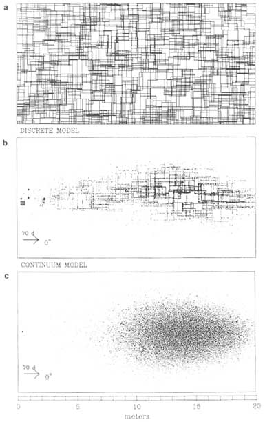
fluid. In these cases, fracture statistics may provide a poor basis for the prediction of flow behavior.
To address these concerns, discrete network models can be extended (1) to take into consideration the origin of the fractures and any statistical distribution functions arising naturally from the mechanics of fracture formation, (2) to incorporate a hierarchical structure of fractures, and (3) to be conditioned on hydrological observations. The term hierarchical refers to a superposition of fractures of many different sizes, with some genetic relationship among the different scales. The term nested structure is analogous to a hierarchical structure. Each scale influences to a varying degree the hydraulic and mechanical behavior of the rock mass. Some means also is needed to identify the more important fractures and to build the geometric model of the network with the emphasis on those fractures. The concept of conditioning discrete network models on hydrological observations usually involves an extension to cross-hole hydraulic tests from the single-borehole tests used in estimating fracture transmissivity.
Rules describing the scale dependence of the hydraulic and transport properties of geological media are being actively explored by the research community. While the discussion of scale-dependent properties is presented here in the context of discrete network models, this topic has a base that extends to all porous media. There is strong evidence from field observations of flow and transport that permeability and dispersivity vary with the scale of measurement. Several models have been suggested to represent this dependence. For example, Neuman (1990, 1994) proposed scaling relationships that treat both porous and fractured rocks as multiscale random functions defined over a continuum. We do not review this broader research issue, but the reader should be aware that these concepts underlie the application of any of the network models presented here.
Geological Evidence of Scale-Dependent Properties
There are several reasons fracture networks might be expected to have scale-dependent or hierarchical properties. Fractures are normally generated in a series of geological episodes. Each succeeding episode of fracturing is influenced by the presence of fractures formed during earlier events because of their impact on the local stress distribution and on rock strength. Dynamic systems of this type are known to produce fractal structures (Barnsley, 1988), In particular, fracture growth has been shown to depend on fracture length (e.g., Griffith, 1920; Pollard and Aydin, 1988). This relationship can lead to systems with a small number of very large features and larger numbers of smaller features, that is, features of every length scale. The implication is that the larger the domain, the larger the features one will observe. The challenge in modeling fluid flow is to include scaling in the description of fracture system geometry.
Tchalenko (1970) showed that fracture systems associated with shear zones are qualitatively similar across a wide range of scales, from tectonic faults of
kilometer-scale dimensions to fractured clay laboratory samples of centimeter scale. The similarities in structure of the fractures were interpreted by Tchalenko as indicating similarities in the deformation mechanism over this wide range of scales. In a similar manner, Martel et al. (1988) showed how the development of fault zones in the Sierra Nevada leads to the formation of several generations of fractures, each related to its parent in a similar way (see Figure 2.18).
Faults are composed of one or many interconnected fractures. At some scales, a fault may appear to be a one-dimensional trace of a single fracture, whereas at another scale the same fault may appear to consist of a two-dimensional set of interconnected subparallel fractures. A number of studies have focused on the irregularity of fault traces at a variety of scales (e.g., Scholz and Aviles, 1986; Aviles et al., 1987; Okubo and Aki, 1987; Power et al., 1987; Hirata, 1989; Power and Tullis, 1991). The basic conclusion of these studies is that single fault traces have topographies that can be described by fractal geometry. When a fault consists of multiple fractures, the fracture system has a fractal character as well.
The fractal concept incorporates scaling and hierarchical structure at a fundamental level. Measurements of the fractal geometry of fracture systems have become more common in recent years (e.g., Barton and Larsen, 1985). Analyses to date have been carried out on linear transects or planar sections of fracture systems. Most studies find power law (fractal) scaling over a wide range of length scales. LaPointe (1988) found that the fractal dimension varied with the orientation of the sample line. A comprehensive review of this work is given by Barton (1995).
In studies of scale-dependent properties, two approaches have been taken. The most common approach is to consider a statistical distribution function—say, the number of fractures in a population as a function of fracture size or the number of fractures observed along a linear transect or a drill core. This approach ignores the spatial position of the fractures and therefore the spatial correlation structure. One study analyzed data on the spatial distribution of fracture density in the form of a "surface topography" and found a power law relationship reminiscent of fractal geometry (LaPointe, 1988). In light of the anticipated importance of spatial correlation in fracture density on fluid flow and transport, the approach of LaPointe is perhaps of greater relevance in hydrological studies.
The evidence suggests that the concept of hierarchical systems is applicable to many fractured rocks. The question remains, in adopting a discrete network model, of how to generate network models that provide a realistic portrayal of these spatial structures.
Geometric Models Incorporating Spatial Relationships Between Neighboring Fractures
The network models described in earlier in this chapter apply to systems in which the fractures are distributed in the rock mass in a more or less uniform pattern. Here we account for fracture patterns that exhibit a spatial dependence
between neighboring fractures. Maps of fracture traces suggest that fracture occurrence is not independent and that fractures tend to occur in clusters. Causative mechanisms for this clustering were discussed in Chapter 2. Two approaches have been pursued: one in which a simple stochastic rule is applied to establish fracture clusters and a second in which an attempt is made to mimic the processes of fracture formation and growth.
Geometric Models Incorporating Clustering of Fractures
Long and Billaux (1987) and Billaux et al. (1989) attempted to include fracture clustering by introducing both a "mother-daughter" process for fracture spacing and an empirical variogram for fracture orientation. A network is built by first creating parent points according to a Poisson process with rate ![]() p where
p where ![]() p varies in space. Once the parent points are placed, a random number of daughters are randomly placed about the parents. Fractures are assumed to occur with their centers at the daughter points. Figure 6.21 presents an example of a fracture network generated by using the parent-daughter process. The clustering of fractures and the scale dependence in the system are apparent. Estimation of the parameters of this model, using data from fracture trace mapping, is illustrated in Billaux et al. (1989).
p varies in space. Once the parent points are placed, a random number of daughters are randomly placed about the parents. Fractures are assumed to occur with their centers at the daughter points. Figure 6.21 presents an example of a fracture network generated by using the parent-daughter process. The clustering of fractures and the scale dependence in the system are apparent. Estimation of the parameters of this model, using data from fracture trace mapping, is illustrated in Billaux et al. (1989).
The parameters of the parent-daughter process were derived by comparing the variogram derived from the field data with a series of theoretical variograms derived from different sets of parent-daughter parameters. An optimization procedure was used to find the theoretical variogram that matched the observed one. Hydraulic data were used to estimate fracture transmissivities. However, this model fails to reproduce the lack of fracture interconnectivity for the same reason as described above by Cacas et al. (1990).
Geier et al. (1989) summarized several models that are similar in intent to the parent-daughter models are:
-
The Levy-Lee model, where fracture centers are generated sequentially using a power law expression for the spacing, with the size of a fracture being proportional to its distance from the preceding fracture.
-
The "nearest-neighbor" model, in which primary, secondary, and tertiary fractures are generated in sequence. Fractures in the primary group dominate the generation of fractures in succeeding groups. Spatial density of the secondary fractures is proportional to the reciprocal of the distance to the nearest fracture.
-
The "war zone" model, in which the spatial density of secondary fractures is greater in the regions between pairs of neighboring primary fractures that are subparallel.
Drift 2
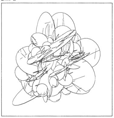
FIGURE 6.21 Example of a fracture network generated by using the parent-daughter process. From Billaux et al. (1989).
Geometric Models Based on Fracture Mechanics
Conrad and Jacquin (1975) were the first to present a two-stage fracture model designed to discriminate between fracture sets in which the fracture traces are extensive and those sets in which the fractures have an irregular pattern and truncate against the extensive fractures. These authors modeled the extensive or primary fractures as unbounded Poisson lines. In the polygons formed by the Poisson lines, finite-length fractures were generated as another series of Poisson points. These fractures were terminated where they intersected primary fractures.
Lee et al. (1990) used the Conrad-Jaquin concept of fracture hierarchy to represent different fracture patterns as they occur in nature. In this so-called hierarchical fracture trace model, fracture trace sets are modeled in a hierarchical (sequential) manner that corresponds to geological processes. Specifically, for
the case shown in Figure 6.22, the first fracture set was produced by a doubly stochastic (Cox) point process combined with an appropriate trace length and orientation distribution model; spatial correlation of trace length and orientation were considered. Fractures were thus reproduced with the appropriate lengths and clustered as in reality. The second set was created by first checking fracture independence in the first set. In case of independence, the second set was created like the first one. In the case of dependence, an appropriate correlation was considered. Also, the observed termination distribution of fractures of one set against those of the other was considered. This model has been validated against real patterns (Figure 6.22).
Geometric models of fracture networks can also be built in a way that mimics the natural genesis of fractures. If this is done alteratively, with each stage of fracturing depending on the results of the previous stage, hierarchical fracture systems can be obtained. There are a number of examples of fracture genesis models based on the physics of fracture growth—for example, Takayasu (1985), Termonia and Meakin (1986), Cox and Paterson (1989), and the references provided therein. As discussed in Chapter 2, Olson (1991) developed a model for joint formation based on continuum mechanics and linear elastic fracture mechanics that included interactions between fractures. It was shown that the crack propagation velocity determined the character of the resulting fracture system. Faster crack growth favors longer fractures formed in clusters, whereas slower crack growth results in fractures of more equal length that are equally spaced. For these models, observation of fracture patterns can help determine the parameters that govern crack growth.
A heuristic model based on the physics of fracture formation has been developed by Martel et al. (1991; see also Long et al., 1992a). Small starter cracks are placed according to a Poisson process. The cracks then grow in a recursive manner according to stochastic rules (Figure 6.23). The rules for growth are based on principles of fracture mechanics and assume that the probability of fracture growth depends on the rate of energy release as a fracture propagates. For an opening-mode fracture, the energy release rate is proportional to the square of the mode I stress intensity factor (Lawn and Wilshaw, 1975). As described in Chapter 2, the stress intensity factor for a uniformly loaded fracture scales with the square root of the length of the fracture. Accordingly, the probability of fracture growth would depend on the first power of fracture length. Principles of fracture mechanics together with experimental findings indicate that under a given load a fracture will propagate spontaneously once it reaches a critical length; below that length it will propagate more slowly, at subcritical rates.
At each iteration a fracture is assigned a probability of growing that is proportional to its length, if its length is less than some critical value, Lc. Above this critical length, all fractures have a probability of growing equal to unity. The amount of growth at each iteration is chosen randomly from a uniform distribution between zero and a maximum growth increment, B = ΔL/L, where
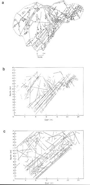
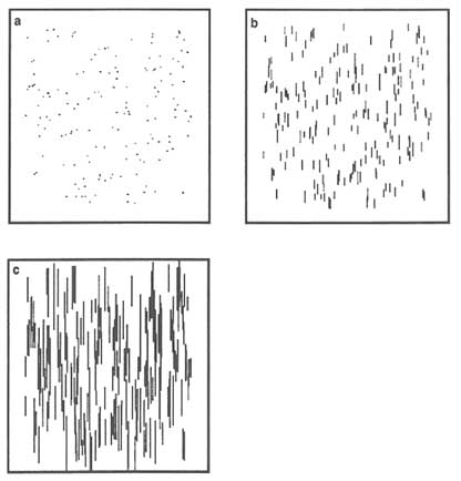
FIGURE 6.23 Development of a fracture pattern from 200 randomly located starter cracks. From Martel et al. (1991).
L is the fracture length. Thus, the choice of B is equivalent to choosing the fracture propagation rate. If fracture growth occurs, either a daughter crack can grow or the parent itself can grow. The probability of daughter versus parent growth, Pd, is a parameter of the model. The entire fracture pattern is thus determined by five parameters: Lc, B, Pd, the number of starting cracks, and the number of iterations.
Flow and Transport Models
The networks created by incorporating spatial relationships between neighboring fractures typically have a wide range of trace lengths. In principle, there is no conceptual difficulty in applying discrete network models to fractures with
multiple length scales. The method, however, can be inefficient because of the high proportion of smaller-scale fractures that are typically generated. To reduce computational requirements when solving the flow and transport equations, a common approach is to simply remove fractures from the network. For example, all fractures with a transmissivity less than the mean might be eliminated on the grounds that they do not contribute significantly to the flux through the network. Hestir and Long (1990) showed that a proportion of the shortest fractures can be eliminated without changing the fracture network permeability.
Smith et al. (1990) describe a simulation approach that recognizes a hierarchy among fractures, preserving dominant fractures as discrete features (primary fractures) and modeling flow and transport in the more numerous, smaller-scale fractures by using a lumped parameter representation (to form so-called network blocks). This concept is illustrated in Figure 6.24. The network blocks are not modeled on the basis of a porous medium approximation. Rather, each network block has unique properties, in the same sense as the primary fractures. Their properties reflect the influence of the smaller-scale fractures that are grouped into the network blocks. This approach is suited to systems where fractures exhibit multiple length scales because it does not ignore the connectivity provided by the smaller-scale fractures while permitting simulation of larger-scale flow systems (Clemo, 1994).
Discrete Network Flow Models Conditioned on Hydraulic Behavior
As discussed earlier, geometric information from fracture statistics does not form a sufficient basis to construct a discrete network model. Hydraulic data must be available to define transmissivities at the scale of individual fractures. Such data are normally obtained from packer tests in single boreholes. One approach to ensure that the constructed network behaves like the real system is to condition the fracture network models using hydraulic data.
Equivalent Discontinuum Models
In an equivalent discontinuum model, flow in fractures is modeled as flow in a set of equivalent conductors, which may be regularized to lie on some form of a lattice (Odling and Webman, 1991; Long, 1993). The lattice is chosen during the formulation of the conceptual model. For example, if fracture zones are found to be the most important flow paths, as at the Stripa mine, the lattices can be confined to the planes (or slabs) representing the fracture zones. In this case the model does not explicitly include every fracture at the site but only a set of equivalent conductors in the fracture zones. In other cases it may be appropriate to construct the lattice throughout the three-dimensional space of the site. If fracture orientation is known, lattice elements can be oriented parallel to the mean orientations of the fracture sets. If the geological investigation suggests
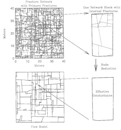
FIGURE 6.24 Division of a fracture network into primary fractures and network blocks. Primary fractures are retained as individual discrete fractures. Most fractures are grouped into network blocks, as shown for the single block that has been isolated in this schematic representation. Modified from Clemo (1994).
that the fracture zones have higher vertical hydraulic conductivities, as in the K-zone at Grimsel in Switzerland, the lattice can be chosen to have vertical elements. The lattice includes any information derived a priori from the characterization process (see ''Development of Conceptual and Mathematical Models," earlier in this chapter) and, in a sense, represents the conceptual model of the site.
Figure 6.25 shows a lattice developed for the Stripa Site Characterization and Validation Project (see Chapter 8). Each plane represents a major fracture zone that, in turn, contains a lattice. The equivalent discontinuum model is similar to an equivalent continuum model, except that some lattice elements are removed.
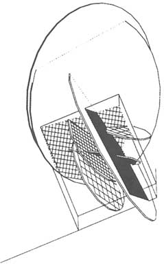
FIGURE 6.25 Three-dimensional template for an equivalent discontinuum model, from the Stripa Site Characterization Validation Project. The features shown are the seven fracture zones identified in Black et al. (1991). Each zone is represented as a disk and contains a lattice. From Long et al. (1992b).
The equivalent discontinuum model is essentially a partially filled lattice that exhibits the same hydraulic behavior as that observed in situ. Where the fracture flow system is connected, the model is connected through lattice elements. Where the flow system is unconnected, the lattice elements are unconnected. Partially filled lattices of this sort have fractal properties near the percolation threshold (Orbach, 1986). The advantages of an equivalent discontinuum model are that it represents the important larger-scale features explicitly and uses equivalent conductors to represent the average behavior of less important features. It is possible to use these models to reproduce the discontinuous hydraulic behavior of a fracture system without modeling every fracture.
An inversion technique called simulated annealing can be used to construct equivalent discontinuum models (Long, 1993). Simulated annealing is an optimization algorithm that finds lattice configurations that are functionally equivalent
to the observed system (i.e., a model that simulates the field behavior). To search for configurations that behave like the observed system, the simulated annealing algorithm makes a random change in the lattice. For example, a lattice element that was on may be turned off (i.e., it becomes nonconducting). For each trial configuration a well test that was conducted in the field is simulated. The "energy" of the configuration is a function of the squared difference between the observed and simulated responses. The problem of finding the "best" model then becomes one of finding configurations that have low values of the energy function. The algorithm accepts the change to the configuration if the energy is decreased over the previous configuration. If the energy is increased, the algorithm may accept the change with a probability inversely proportional to the energy increase. Thus, the solution "wiggles'' out of local minima and can find the globally minimum solution.
An example of equivalent discontinuum modeling at the Stripa mine is provided by Long et al. (1992b). A fracture zone at the mine called the H-zone was intersected by a series of wells (W1, W2, C1–C5, D1–D6). Hydraulic interference testing was carried out. A two-dimensional lattice template was constructed for the H-zone. The template was designed (1) to represent as much detail as possible in the vicinity of the D-holes, (2) to have a large enough mesh to prevent the hydraulic disturbance from reaching the boundary too quickly, and (3) to keep the number of elements and bandwidth as small as possible for efficient annealing.
The total inflow to the six parallel D-boreholes (D1–D6) from the H-zone was modeled using simulated annealing. Simulated annealing produces a model that matches an interference test called the C1–C2 large-scale cross-hole test, which was conducted by pumping from the H-zone in well C1 and monitoring the other boreholes. The "best-fitting" model is shown in Figure 6.26. The annealed network is analogous to a finite-difference model of a continuum with variable connectivities, more so than being representative of actual fractures. The grid does, however, provide an explicit representation of the connectivity (or lack of connectivity) in the fracture zone. Figure 6.27 shows the match between the observed well responses and the model responses. The mesh was adjusted to calculate the effects of opening the D holes and collecting the inflow. The measured steady-state flow (0.75 liters per minute) and the predicted value (0.77 liters per minute) agree quite well.
Emerging Concepts
For fracture networks near the percolation threshold, the equivalent discontinuum models described above result in a fractal structure through the development of a percolation lattice. Several attempts have been made to model fracture systems using numerical approximations of fractals directly. Pollek (1990) built a series of random Sierpinski's gasket models with various fractal dimensions
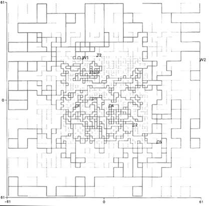
FIGURE 6.26 Two-dimensional equivalent discontinuum model of the H zone at Stripa, annealed to C1–C2 cross-hole hydraulic test. From Long et al. (1992b).
and compared the behavior of well tests on these models to the behavior predicted by Barker (1988). Chang and Yortsos (1990) derived solutions for well test behavior on fractals, in this case fractals embedded in a porous matrix, thus explicitly addressing systems with both fracture and matrix porosity. Acuna and Yortsos (1991) constructed approximate numerical models of this fractal system to compare the well test behavior with that derived by Chang and Yortsos.
Another emerging concept involves the use of an iterated function system (IFS), which is a standard way to model self-similar geometrical structures (Barnsley, 1988). An IFS comprises an initial set of points and a set of iterative functions. At each iteration, each function in the system operates on the set of points and, according to the parameters in the function, translates, reflects, rotates, contracts, or distorts them. Over many iterations the points coalesce toward an "attractor." The IFS is designed such that the attractor is a fractal object.
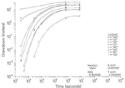
FIGURE 6.27 Comparison of the C1–C2 well test response data to the prediction of these test results provided by the equivalent discontinuum model. From Long et al. (1996).
An IFS can be used as the basis of hydrological inversion (Doughty et al., 1994; Long et al., 1996). In this case the points of the attractor are mapped into hydrological parameters (i.e., conductivity and storativity) and used to simulate a well test. For example, an attractor can be superimposed on a lattice by incrementing the conductance and storativity of the lattice elements that are close to each point on the attractor, as shown in Figure 6.28. The conductance of a lattice element can be incremented as many times as there are nearby points on the attractor. In this way the small number of parameters of an IFS defines the conductance and storativity distribution of thousands of elements.
One of the potential advantages of this approach is that it may be possible to choose subclasses of IFSs that produce features observed in a geological investigation. For example, it may be possible to find IFSs that always produce cooling fractures or a specific type of brittle shear zone. In these cases the search for appropriate models could be confined to the subclass of IFS that represents that geology. Once the form of the IFS that best explains all the data has been identified, the model will have fractal-like properties that may help to extrapolate behavior to scales that cannot be tested in reasonable time frames.
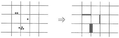
FIGURE 6.28 Step mapping between points on the attractor and increments in hydrological properties of the lattice. This example is for incrementing conductance. Points can also be used to decrement conductance. From Doughty et al. (1994).
Inverse methods applied to fractal models can be used in a manner similar to that for an equivalent discontinuum model. An inversion algorithm searches for IFS parameters that define a heterogenous system that behaves like the observed well tests. Starting with a model of the flow system based on an arbitrary IFS, the parameters of the IFS are optimized until the model produces a good match to the well test data. The advantage of the IFS inversion is that the whole system is defined by the small number of parameters that define the IFS. Consequently, there are fewer degrees of freedom in the inversion. Figure 6.29 shows preliminary models of the H zone at the Stripa mine constructed through IFS inversion using the same data as the model in Figure 6.26.
Recently, interest has been growing in neural network models. In this approach a whole series of specified conditions and outcomes are used to "teach" the neural network, which may be thought of as a "black box" of how the system works. Then, when new conditions arise, the neural network uses its "understanding" to predict system behavior. This approach can be used without even trying to define a model for the system. The approach can be purely heuristic, which may be particularly useful when hydrological data are available, but there is little information about the configuration of the fracture system. On the other hand, the approach may also involve physical understanding. This line of research is worthy of more attention.
Assessment of Scale-Dependent Discrete Fracture Models
The work on fracture growth schemes shows promise of being able to reproduce fracture patterns. The development of physically based stochastic models of fractures is an important area of research. The advantages to be gained from such models are numerous. First, the model has quantifiable parameters whose values can be estimated from observations of the fracture system. Because the model is physically based, knowledge of these parameters can aid the geologist in further understanding the fracture formation process. Second, the model param-
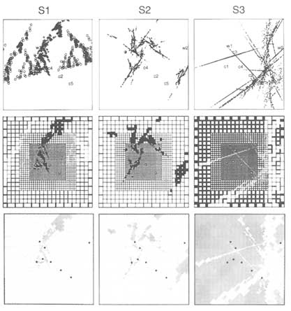
FIGURE 6.29 IFS inversion of an interference test in a fracture zone (H zone) at Stripa. Top row shows three different attractors from three different IFS schemes: left figure is for the case that the IFS increments permeability; middle figure is for incrementing and decrementing; and right figure shows the attractor for decrementing permeability. Middle row shows the resulting numerical grid. Higher conductances are shown by thicker lines. Bottom row is the average distribution of conductance that results from the attractor. Lighter colors represent lower conductances. From Doughty et al. (1994).
eter estimation scheme can be used to guide the collections of field data appropriate to understand the fracture system. Finally, uncertainties about the model parameters can be used to estimate uncertainties about fracture system geometry.
The idea of using cross-hole hydraulic tests to calibrate discrete network models also appears promising. Reliable hydraulic test data can be used with inversion methods to find permissible configurations for the conducting lattice. In practice, however, it can be quite difficult to obtain a good data set for analysis.
Some of the difficulties arise from the usual problems with model calibration, for example, poorly known boundary conditions and incomplete or insufficient data. Other difficulties arise because the inversion procedure must be tailored to the specific type of test data available (e.g., steady-state or transient tests).
In general, the inversion of hydraulic test data yields nonunique solutions. The problem is compounded by the generally limited availability of data. Characterization efforts must recognize from the beginning this nonuniqueness problem. If several different hydraulic well tests are available to calibrate the model, they can be combined. In principle, any combination of steady-state test data, constant flow, or constant-head transient data can be cointerpreted by the inversion. The advantage of using multiple-well tests is that each additional test provides more information about the system. Preliminary work with simulated annealing indicates that predictions based on two-well tests are significantly better than those based on one-well tests. The main drawback for combining a large number of transient tests is the potential computing requirements.
Efficient computer algorithms are being developed that may help to make simulated annealing a practical tool. Another important effort is to improve the efficiency of solution searches. For example, a priori information, such as geophysical data, can be incorporated to force the search to look for permeability anomalies where there are geophysical anomalies. Coinversion of both geophysical data and hydrological data might also be useful. Geophysical data should be used as a priori information because a significant amount of expert judgment is needed to interpret such data. This judgment would be overlooked in a coinversion.
MODELS OF MORE COMPLEX HYDROGEOLOGICAL SYSTEMS
Much of this chapter has been devoted to problems involving saturated isothermal flow in nondeforming rock masses, or the transport of nonreactive solutes. These conditions encompass a wide range of problems encountered in practice, but there are many situations where these assumptions are not valid. Examples include the disposal of radioactive waste in the unsaturated zone above the water table, migration of multiphase organic contaminants, and heat extraction from hot dry rock systems. The following review of modeling techniques for these kinds of problems is not exhaustive. Indeed, as these problems commonly involve systems of great complexity, there are significant gaps in our capabilities to model these systems at field scales. Nonlinear relationships between the media properties that characterize the conductance of a fractured rock mass and the degree of phase saturation are very difficult to quantify at field scales. Coupling between the thermal, hydrogeological, mechanical, and geochemical systems also is characteristic of these more complicated systems (see de Marsily, 1987). The objective of this section is to highlight certain issues and concerns that arise when formulating conceptual models and simulation for these more complex systems.
Modeling Flow and Transport in the Unsaturated Zone
Comprehensive research programs to investigate fluid flow and solute transport in unsaturated fractured rock have only recently been organized. The impetus to better understand the processes involved, and to develop a simulation capability, comes primarily from two sources: (1) the U.S. Department of Energy's program to evaluate the vadose zone at Yucca Mountain, Nevada, as a potential site for a high-level radioactive waste repository and (2) siting efforts for landfills and other surface-based disposal facilities in regions with deep unsaturated zones. There have been a number of refinements in conceptual models of flow in these regions. However, comprehensive understanding of the mechanisms of fluid flow in unsaturated fractured rock, matrix-fracture interactions, and spatial-temporal recharge fluxes through the vadose zone has yet to be developed. A collection of papers edited by Evans and Nicholson (1987) provides a good review of the state of the science to the mid-1980s.
In its most complete form, movement of water in unsaturated fractured rock is a problem of multiphase fluid flow (water and air phases), with the pressures in one phase influencing the mobility of the other phase. The complexity of the problem is reduced if it is assumed that the air phase is immobile and exists at constant pressure throughout the domain of interest. This approximation is routinely made in modeling water movement in unsaturated porous media.
Under conditions of partial saturation, capillary forces influence the subsurface distribution of water. Fluid saturation and hydraulic conductivity are functions of moisture content and, thus, fluid pressure. The conceptual model of fluid flow that is favored by some workers is illustrated in Figure 6.30. Fractures with larger apertures tend to desaturate before pores in the matrix blocks, so connected pathways for fluid flow will preferentially be located in the matrix blocks, with flow occurring across the fractures only at contact points (Wang and Narasimhan, 1985). As a consequence, drained fractures may act as a barrier to the infiltration of a wetting front, a reversal of the situation that occurs in the saturated zone. As water saturation increases, a limited number of connected pathways will be established along the fracture planes, especially in the smaller-aperture fractures. Once saturated, the highest fluid flux will be through the connected fracture network.
It is becoming apparent through theoretical and laboratory studies (Chapter 3) that there may be significant phase interference in fractures under conditions of unsaturated flow. In a planar fracture, when the matrix rock is relatively impermeable, the fracture behaves essentially as a two-dimensional porous medium. Under two-phase conditions, the presence of the second phase in the plane of the fracture can create barriers to the flow of the first phase, and vice versa. Since these fluids cannot use the third dimension (i.e., the matrix) to find flow paths around the other phase, the flow may be even more channelized than under conditions of saturated flow. The active flow region in the fracture may
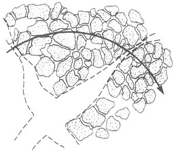
FIGURE 6.30 Conceptual model of flow in an unsaturated fractured rock. From Wang and Narasimhan (1985).
be so small that little of the phase will be drawn into the rock matrix by capillary forces. If the fracture surfaces are sealed with minerals and the rock matrix is near saturation, downward flow to the water table may be largely confined to the fractures. A conceptual model of this system would differ significantly from the conventional view of unsaturated flow in fractured rock, which predicts that the matrix controls the flow and that fractures act as barriers to it. Indeed, this conceptual model would predict a more rapid downward transmission of fluid than the conventional model, where flow is confined to the rock matrix.
These two models describing infiltration through the vadose zone may be operative at different times as surface hydrological conditions change. The conventional model assumes that the connected fractures are drained and that water moving downward does so through matrix blocks where moisture contents and permeabilities are higher. The alternative model is based on downward infiltration through fractures, which might occur during precipitation events that promote saturation of the fractures at the ground surface. The wetting front in the connected fracture network need not coincide with that in the rock matrix. The depth of penetration of the wetting front is a complex function of fracture and matrix geometries, moisture contents, and permeability of the fracture wall.
Evidence for these two modes can be found at the Apache Leap research site in Arizona, where data suggest that recharge through unsaturated tuff occurs
along two pathways, one through fractures and the other predominantly through the rock matrix. Intermittent pulses of stream seepage penetrate to a tunnel 150 m below the ground surface in a matter of days to weeks. On an adjacent escarpment at a similar depth, geochemical evidence indicates that much older water occurs in a perched zone. It has not yet been possible to determine the percentage of the recharge to the perched zone that follows fracture and matrix-dominated pathways. At the Apache Leap site Rasmussen and Evans (1993) have demonstrated the possibility of high water intake rates on exposed fractured rock surfaces.
Two-phase flow in a fracture may never be truly steady state. Even under steady-state boundary conditions, pressure in the wetting phase will build up, eventually causing the wetting phase to displace the nonwetting phase occupying the larger, more permeable void spaces in the fracture plane. Subsequently, the pressure dissipates and the wetting phase is swept out again. Such oscillatory flow has been observed in the laboratory (Persoff et al., 1991) and possibly in the field (Olsson, 1992). A key area for research is to determine if the amplitude and period of this oscillatory flow behavior increase with the scale of the flow system as might be expected.
Rasmussen (1991) describes a technique for modeling steady-state fluid flow and advective transport in a partially saturated fracture network embedded in impermeable rock. The technique utilizes a discrete air-water interface in each fracture to separate the saturated region from the drained region. A similar approach uses accessibility and allowability criteria to determine which fractures in a network will contain water and which will contain air (personal communication, Kenzi Karasaki, Ernest Orlando Lawrence Berkeley National Laboratory). Therrien (1992) has developed an efficient three-dimensional, discrete fracture model that solves for variably saturated ground-water flow and solute transport. The matrix blocks between the discrete fractures are porous and permeable. Complex interactions caused by contrasts between the saturation, relative permeability, and pressure-head relationships for the fractures and the matrix control the redistribution of water in the system. Depending on the nature of these relationships, groundwater flow and solute transport can be controlled either by the porous matrix or the fractures. Fracture connectivity in three dimensions shown to produce very irregular hydraulic-head patterns in fractured aquitards, which can lead to the development of irregularly shaped contaminant distributions in the subsurface.
It is not known how well conventional unsaturated flow models based on porous medium approximations represent flow processes in the vadose zone. Few studies have examined how best to average the properties of the matrix and the fractures under conditions of partial saturation (Figure 6.31). The work of Peters and Klavetter (1988) is an important step forward in addressing these issues. If the majority of fractures are drained, the moisture content versus pressure head and permeability versus moisture content relationships are determined by the properties of the matrix blocks. Under these conditions it seems probable that
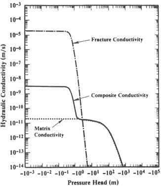
FIGURE 6.31 Hydraulic conductivity of unsaturated fractured volcanic tuff from Yucca Mountain, Nevada, plotted as a function of fluid potential. Pressure values are negative, indicating that water is held in tension. From Peters and Klavetter (1988).
continuum approximations are valid. At near saturation, connected pathways through smaller-aperture fractures may develop, potentially leading to substantial increases in rock mass permeability. Properties of the fracture network will determine fluid fluxes, and the same concerns discussed earlier about continuum approximations under saturated conditions are applicable.
To model fluid flow in unsaturated fractured rocks using currently available models, relationships must be developed for moisture content, fluid pressure, and relative permeability. Additional data are needed to develop relationships for fluid exchange between the fractures and the matrix blocks. Even in a single rock type with a uniform fracture geometry, measurements of characteristic curves representative of field-scale behavior are difficult to obtain. This issue is explored by Kwicklis and Healy (1993), using a numerical model of steady flow through a variably saturated fracture network.
Only limited work has been completed to examine how best to average the properties of the matrix and the fractures under conditions of partial saturation. In a domain containing different lithologies or spatially variable fracture geometries, data requirements seem immense. There is again the issue of how measurements made at one scale can be extended to characterize flow behavior at other scales. At scales of tens to hundreds of meters, parameter estimates may best be constrained through model calibrations using geochemical or isotopic indicators.
Modeling Multiphase Flow in Fractured Rocks
Models that simulate multiphase flow in fractured rock systems arise in petroleum reservoir engineering, in the analysis and development of some geothermal systems, and in contaminant hydrogeology. Experience with multiphase flow models has been considerably more extensive in the petroleum engineering field than in the field of groundwater hydrology. Although the models in both fields have a common basis in the physics of immiscible fluids, they address different sets of problems. For example, interest in fractured petroleum reservoirs commonly centers on prediction of oil displacement from matrix blocks under various recovery plans. Predicted pressure changes in each fluid phase are key variables in characterizing reservoir performance. In geothermal systems the phases of interest are steam and water, and an important area of concern is the generation and migration of steam with a decline in the reservoir pressure. In environmental applications an important issue concerns the redistribution of an organic solvent in a water-saturated medium that initially contains none of this phase. In this case the interest is in the spatial extent and distribution of solvent in the subsurface.
Simulation of multiphase flow (e.g., oil/water/gas) in a naturally fractured petroleum reservoir is normally carried out by using continuum approximations embodied in a dual-porosity model. A mature literature exists on this topic, and Kazemi and Gilman (1993) provide a recent overview of the models used in the petroleum industry. Balance equations are written for each fluid phase, for flow in both the fracture network and the matrix blocks. Because this is a continuum approximation based on porous medium equivalence, rates of fluid flux and capillary pressure are expressed in terms of relative permeability and phase saturation, respectively, for each of the fracture network and matrix domains.
For cases where significant fluid flow occurs between matrix blocks, the dual-porosity model has been extended to produce what are known as dual-permeability models. The fracture network and matrix blocks are viewed as two superimposed continuua, with both the fractures and the matrix forming continuous flow paths across the reservoir. Balance equations are written for multiphase flow in both the fracture network and the rock matrix. This model differs from the dual-porosity model by the addition of interblock matrix flow terms. If these additional terms are set to zero, the dual-porosity formulation is recovered. The concerns raised earlier (''Dual-Porosity Models") about the
predictive capabilities of dual-porosity models are also appropriate when discussing multiphase flow.
The escape of synthetic organic liquids (nonaqueous-phase liquids, or NAPLs) to the subsurface environment poses a significant threat to groundwater quality. Although NAPLs are typically of low solubilities, their dissolution can lead to aqueous-phase concentrations far above drinking water standards. Migration of NAPLs as a separate phase effectively creates a much larger source volume from which mass can be transferred to the aqueous phase by dissolution. The capability to make site-specific predictions of the movement of NAPLs through fractured porous media does not exist with current modeling tools.
Most NAPLs behave as nonwetting fluids, preferentially occupying the larger void spaces. The low viscosity of some NAPLs enhances their mobility. If the fluid density of a NAPL is less than that of water (e.g., gasoline), it will move downward through the vadose zone to the water table, at which point it will migrate laterally. Some fraction of the NAPL will be left behind in fractures in the rock as a residual saturation. Dense NAPLs (e.g., trichloroethylene or polychlorinated biphenyls [PCBs]) can penetrate the water table, moving downward and laterally in a pattern strongly influenced by geological structure. At sites underlain by fractured rock with low matrix porosity, the potential exists for substantial vertical and lateral migration of an NAPL as a separate phase.
Chapter 3 addresses multiphase flow at the scale of a single, rough-walled fracture. For the field problem it is necessary to extend the observations made in single fractures to models that characterize flow in an interconnected network of fractures. A conceptual model of NAPL movement in a fractured medium is shown in Figure 6.32. An NAPL will enter a water-saturated fracture only if the capillary pressure at the entrance to the fracture is greater than the entry pressure. Entry pressures are smaller for larger-aperture fractures or along segments of a fracture where the aperture is greater. The geometric properties of a fracture network are critical factors in determining large-scale migration patterns. At the local scale, NAPLs may be distributed in a very irregular manner. Perhaps the issue of greatest theoretical concern is the determination of appropriate scaling relationships for describing capillary pressure saturation and relative permeability curves at the scale of a fracture network from measurements on single fractures or blocks containing a small number of fractures.
Multiphase flow models describing NAPL migration in fractured rock could be used in practice to provide much-needed insights into physical (and chemical) processes for NAPL migration at the network scale. With respect to site-specific applications, models may have two uses. One is to estimate migration paths and the subsurface volume of residual NAPL for the design of site investigation programs. A second use is for evaluating remediation programs to remove NAPL from a fractured porous medium. However, even as the numerical capability for simulation emerges, it is unclear whether data requirements and the high sensitivity
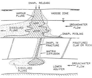
FIGURE 6.32 Conceptual model describing movement of a dense nonaqueous-phase liquid (DNAPL) downward across a fractured geological unit. The liquid has a density greater than that of the groundwater. From Kueper and McWhorter (1991).
Chemical Processes
The hydrological processes that transport dissolved solutes through an open fracture network are linked to chemical processes in the geochemical environment that act to modify solute concentrations. Perturbations of the thermal or stress regime may also initiate and maintain chemical reactions. Flow and transport of reactive solutes are a complex nonlinear system that is difficult to analyze quantitatively.
Chemical processes of interest include precipitation-dissolution reactions, redox reactions, surface sorption, complexation, and transformations of organic compounds. These reactions can occur in the fluid phase; at the interface with a fracture wall; or, as a result of diffusional mass transfer, in matrix pore spaces adjacent to the fracture. Fluid pathways in fractured media may be quite complex. Mixing of fluid with different chemistries in such media cannot necessarily be understood using conventional porous media concepts.
To account for chemical reactions during transport, a geochemical model must be coupled to the mass balance expressions that are the foundation of the fluid flow and solute transport equations. The choice of geochemical model is very much problem dependent. For example, hydrothermal ore deposits typically reflect mineralization from a relic flow system in a fractured rock. Mineralization commonly occurs as the result of a perturbation in the flow system, for instance, a rapid reduction in fluid pressures owing to fracture dilation. To model this system, fluid flow and transport models must be linked to models of the thermal and stress regimes. Time scales of interest may extend over many thousands of years, with repeated episodes of fracture opening and sealing. In principle, equilibrium speciation models of the type used in porous media simulations can serve to track the evolution of the chemical system. If the rate of advective mass transfer through the fracture network is fast relative to the rates of chemical reactions, kinetic models may be needed. The complexities of such systems are great. A quantitative framework is now emerging as a result of careful geological observation to describe in general terms the dynamic evolution of fracture-dominated hydrothermal systems.
In some ways the transport of reactive solutes away from a hazardous waste site or surface impoundment is simpler to characterize than transport in hydrothermal systems. The time scales of concern are much shorter. The thermal and stress regimes can usually be decoupled from the chemical state of the system. Temperatures and pressures are lower. Simpler geochemical models may serve to approximate the important chemical processes. In other ways the problem is more difficult, because site-specific predictions of the potential for, or extent of, off-site migration must be obtained.
Surface sorption of a trace metal or dissolved organic compound is one of the more straightforward geochemical processes to incorporate into a transport model. For problems involving transport in granular porous media, chemistry is commonly simplified. Linear exchange models are used to represent the reversible transfer of mass between the aqueous phase and the solid surface. Recent experimental evidence does, however, point to limitations in the use of a simple, reversible sorption coefficient (Vandergraaf, 1995).
When modeling geochemical processes in fractured rock, there are a number of concerns related to the geometry of flow. A key concern is determination of the contact area between the solute and the rock matrix (Moreno and Noretnieks, 1993). The contact area depends on the degree to which fluid is channelized along pathways through the fracture network, the extent of surface sorption on the fracture walls, and the access of the solute to the rock matrix. At present, it is not known how to introduce these factors into simulation models, in part because it is not known what should be measured in the field. As frequently noted in this chapter, it is difficult to characterize flow paths at the field scale in fractured rock masses. Wels and Smith (1994) suggest that retardation of solutes at the plume scale is a nonuniform, anisotropic process as a consequence
of the inverse relation between retardation and fracture aperature at the scale of individual fractures. There are also unresolved issues about the size of an averaging volume associated with a continuum approximation when comparing the cases of reactive and nonreactive solutes. Reactive transport is more difficult to simulate if the fractures that control flow (e.g., larger, well connected fractures) do not also control the geochemistry of the system. These issues require additional study, both experimental and theoretical, to provide quantitatively sound methods and models for the prediction of reactive solute transport in fractured geological media.
Modeling Heat Transfer in Fractured Rocks
In low-permeability unfractured rock, conduction is the dominant mechanism of heat transfer. Advection of heat by moving groundwater may dominate heat transfer in highly permeable or fractured rocks. An understanding of advective heat transfer is an important problem in fractured systems, with application in the analysis of geothermal systems, disposal of high-level nuclear waste, and characterization of hydrothermal circulation in the oceanic crust.
To model heat transfer in a fractured porous medium, an energy balance equation is introduced to account for conductive and either convective or advective heat transfer in the fracture network and matrix blocks. The presence of a heat source creates spatial gradients in fluid density that provide an additional driving force for fluid flow and solute transport. Fractures serve as efficient conduits for heat transfer by fluid motion, and matrix blocks can be large reservoirs of thermal energy storage. Heat exchange between the matrix and fracture network depends on rates of fluid flow in each domain and the geometry of the fracture network. The main problem in modeling a geothermal reservoir to assess its production potential is to obtain representative values for the hydrological and thermal properties of the fractured rock mass.
The flow model in a geothermal reservoir simulation may be based on single-phase or multiphase flow, depending on whether temperature and pressure conditions allow the formation of a steam phase. The fluid flow and heat transfer equations are coupled and must be solved either simultaneously or iteratively. Pruess and Wang (1987) and Bodvarsson and Witherspoon (1989) provide recent reviews of geothermal models. Most geothermal reservoir simulation models fall into one of two classes: either the rock mass is treated as a single continuum that reflects the composite properties of fractures and matrix or a double-porosity formulation is chosen. The double-porosity models are simply an extension of the models described earlier for single-phase isothermal flow. Double-porosity models assume a regular fracture geometry. Discrete features such as major through-going faults, which are key elements of many geothermal settings, may be modeled as separate hydrogeological units. Both single- and double-porosity models are based on porous medium equivalence.
Advective heat transfer in geological settings at scales where continuum approximations may not hold is an important and largely unexplored topic. This problem could be approached on a theoretical level by coupling the discrete network flow models described earlier with a heat transfer model for the fracture network and the surrounding rock mass.
SUMMARY
Issues of scale underlie and confound the development of hydrogeological simulation models. Scale issues are particularly troublesome for developing hydrogeological models of fractured media. The main difficulty is the identification and representation of the heterogeneous properties of the connected fracture network. Individual measurements of hydraulic properties in single boreholes or detailed characterization of a rock mass volume are made on a small scale relative to the scale of the simulation model. The most basic issue facing the modeling community is how to use measurements obtained at one scale to estimate model parameters that represent another scale of heterogeneity of a fractured rock mass.
The conceptual model plays a fundamental role in dealing with the issue of scale in flow and transport models. As noted previously, the conceptual model can be viewed as a hypothesis describing the main features of the geology, the hydrological setting, and site-specific relationships between geological structure and patterns of fluid flow. It provides the basis for identifying the most important features of the fracture system that need to be incorporated into the hydrogeological or transport simulation model. The simulation model is simply the mathematical expression of the conceptual model in a form that permits a quantitative assessment of system behavior or system response to perturbations. Given a robust conceptual model of the fracture system, different mathematical formulations of the simulation model will likely give similar results. However, an inappropriate conceptual model can easily lead to predictions that are in error by orders of magnitude.
The modeling process is by its very nature an iterative procedure. The steps in building a conceptual model of a flow system in fractured rock include the identification of important features of the fracture system, their location in the rock mass, and determination of the extent to which they conduct fluid. Geological models of the fracture system are an essential part of conceptual model building. As additional data are collected and analyzed, the conceptual model is revised and the hydrogeological simulation model is updated. In the process of calibrating and testing a hydrogeological simulation model, assumptions and approximations on which the conceptual model is founded can be evaluated and refined, if necessary.
Three basic questions must be addressed before a simulation model can be used as a site-specific design tool. First, does the conceptual model provide an adequate characterization of the hydrological system? Second, how well does the
simulation model compare with competing models based on different modeling concepts or different model structures? Third, is the data base adequate to estimate the simulation model parameters with sufficient reliability that the associated prediction uncertainties are acceptable in light of the intended application of the simulation model in the decision process? If not, additional data collection is justified. It is commonly the case that these questions are considerably more difficult to resolve when dealing with fractured media owing to the greater heterogeneity of the flow system.
The level of detail required in the conceptual model varies with the purpose for which the model is being developed, for example, whether it is being used to predict fluid flow or solute transport. Experience suggests that for volumetric flow predictions can be made with a relatively generalized conceptual model, provided data are available to calibrate the simulation model and average rather than local-scale behavior is required. For problems involving solute transport through fractured rock, a considerably more refined conceptual model is needed, in terms of a description of the fracture flow paths, to develop reliable predictions of travel times or solute concentrations because of the sensitivity of these variables to the heterogeneity of fractured systems.
Simulation models can be classified on the basis of how fracture system heterogeneity is incorporated into the model structure. Deterministic continuum models typically represent the heterogeneity of the fractured rock by using a limited number of regions, each with uniform properties. Individual fractures are not explicitly treated in the model, except when they exist on a scale large enough to be considered a separate hydrological unit. Stochastic continuum models represent the heterogeneity of the fractured rock as a continuous random field, with the scale of heterogeneity tailored to the scale of measurements of permeability made in the field. Discrete network models explicitly include large numbers of individual fractures that conduct fluid in the model structure. They reflect an attempt to represent heterogeneity on a scale smaller than normally considered in a continuum model.
Recent model innovations combine elements of both discrete network and continuum approximations. Within each class of model, the analysis may be structured in either a deterministic or stochastic framework, depending on whether the coefficients that characterize heterogeneity are viewed as being known with certainty (or are used as the most likely values) or are described by probability distributions.
There is a diversity of opinion on which numerical modeling approaches are most useful in practice when considered across a broad range of geological settings, scales of interest, and project budgets. In the committee's view, two points are of fundamental importance. First, it is important that a model capture the pattern of heterogeneity in the rock mass; it is less important which type of numerical model is used for representing fracture permeability. Second, no single modeling approach is superior in all instances. A limited number of model
comparisons have been attempted. In these cases most of the flow and transport data derived from the experiments can be more or less equally interpreted by means of a number of fundamentally different mathematical models. However, the experiments on which models have been compared were not designed to discern between different models.
There is also a diversity of opinion on the principles that should guide selection among competing models. Model selection involves an assessment of data availability (both geological and hydrological data), the style and scale of fracturing and the degree of heterogeneity, data reliability, and the intended application of the model. Progress in this area will come only with the availability of more experimental sites and additional experience in testing model predictions encompassing a variety of fracture styles.
The strength of the continuum approach is that it reduces the geometric complexity of the flow patterns in a fractured rock mass into a mathematical form that is straightforward to implement. Averaging volumes associated with the deterministic continuum approximation must be large enough to encompass a statistically representative sample of the open, connected fractures and their variable influences on flow and transport behavior. Effectively, this means that averaging volumes must be sufficiently large that fluid flux and solute transport are not influenced to any significant degree by any individual fracture or its interconnections with other fractures in the conducting network. For most applications that are encountered in practice, some type of continuum approach remains the preferred alternative. Its two greatest limitations are that (1) the scale at which the continuum approximation is justified can be difficult to quantify and (2) the process of spatial averaging restricts the possibility of making model predictions at scales smaller than that of the representative elemental volume. If averaging volumes are large, there may be a broad class of hydrogeological problems, especially those related to contaminant transport, that are not amenable to analysis with deterministic continuum models.
The stochastic continuum approach is built on a geostatistical representation of the spatial variability in the conductance properties of the rock mass. Its important practical advantage is that it works directly with field measurements of permeability, rather than a suite of parameters characterizing network geometry. The scale at which heterogeneity is described can be tied to the scale of field measurements. Stochastic theories provide equations for estimating larger-scale hydraulic and transport properties from the smaller-scale field measurements (Neuman and Depner, 1988). The validity of the stochastic continuum approach rests on the suitability of approximations embodied in the representation of a fractured rock mass as a heterogeneous porous medium and in the suitability of mathematical simplifications that underlie stochastic transport theory. Additional studies are needed to evaluate the capability of geostatistical models to capture the structure of a conducting fracture network (or the so-called hydraulic backbone
of the rock mass) from a suite of smaller-scale permeability measurements derived from packer tests.
Discrete network models are predicated on the assumption that fluid flow behavior can be predicted from knowledge of the fracture geometry and data on the transmissivity of individual fractures. The guiding principle is that one can measure spatial statistics associated with a fracture network, including fracture transmissivity, and use these statistics to generate realizations of fracture networks with the same spatial properties. The fractures in these realizations become the conductive elements in a fracture network flow or transport model. Discrete network models are closely linked with concepts of stochastic simulation, and they lead naturally to the adoption of Monte Carlo simulation techniques to quantify the magnitude of uncertainties in model predictions. In some circumstances, discrete network models may provide one alternate means of estimating large-scale hydraulic and transport properties of the rock mass for use in equivalent continuum models.
Two classes of models have been proposed to represent the geometric properties of fracture networks. One class is based on the assumption that the occurrence of one fracture has no influence on the positioning of any subsequent fracture that is generated to form the network. The second class of models allows a spatial dependence between the positioning of neighboring fractures and leads to networks with recognizable, scale-dependent characteristics. Both models comprise rules for specifying the location of fractures in space; the shape of fractures; the extent of fractures, including truncations against other fractures; the orientation of fractures; and the conductive properties of fractures.
In cases where an equivalent continuum cannot be defined, a discrete network simulation may be a viable alternative. This approach appears most useful in problems of near-field simulation over length scales of 50 to 100 m. Simulations at larger scales require grouping fractures into single features or elimination of less transmissive fractures. The disadvantages of discrete network simulation are threefold: (1) the method requires statistical information that may be difficult to obtain (e.g., fracture size), (2) the models are complex and computationally intensive for realistic fracture densities, and (3) there is no guarantee that a model reproducing the apparent geometric properties of a fracture network will capture its essential flow or transport features.
Geometric information from fracture statistics is not sufficient to construct a discrete network model. To be useful as a simulation tool, discrete network models must incorporate the information contained in the conceptual model concerning the properties and positions of the hydrologically dominant fractures. Hydraulic data also must be available to define transmissivities at the scale of individual fractures. The magnitude of fluid flow estimates is critically dependent on the values assigned to fracture transmissivity. Mechanical measurements of fracture aperture are of little value in this regard as they do not capture the influence of the internal geometry of the fracture plane on the hydraulic resistance
to flow. The observed fracture pattern may not be strongly related to the hydraulic backbone of the conducting fractures if, for example, a significant percentage of the fractures are sealed by mineral precipitates or closed owing to the stress regime. A model based on fracture occurrence that does not account for nonconductive fractures can vastly overestimate the connectivity of the network and will fail to capture the hydraulic behavior of the rock mass.
The latest developments in the area of discrete network simulation address two of the limitations of is method: (1) there are typically no mechanistic underpinnings to the proposed stochastic structure of the fracture network, and (2) a significant number of the observable fractures may not be open to flow. Discrete network models have been extended (1) to take into consideration the origin of the fractures and any statistical distribution functions arising naturally from the physics of fracture formation, (2) to incorporate a hierarchical structure in representing the fracture system, and (3) to be conditioned on hydrological observations. There are a number of reasons to expect that fracture networks will have scale-dependent or hierarchical properties. Some method is needed to identify the more important fractures in the fracture system and to build the geometric model of the network with the greatest emphasis on those fractures. The concept of conditioning discrete network models on hydrological observations involves an extension to cross-hole hydraulic tests from the single-borehole tests used in estimating fracture transmissivity. In this approach an inverse technique is used to construct a representation of the fracture network that is functionally equivalent to the observed system in the constraints imposed by the conceptual model.
APPENDIX 6.A
MODEL PREDICTION USING A CONTINUUM APPROACH: THE URL DRAWDOWN EXPERIMENT
Since 1980, Atomic Energy of Canada Limited has been developing an Underground Research Laboratory (URL) in southeastern Manitoba (Davison, 1985; see Figure 8.14 for location map). This facility plays a key role in Atomic Energy's research and development program to evaluate the feasibility of geological disposal of radioactive waste in plutonic rocks in the Canadian Shield (see Chapter 8). The laboratory, excavated in crystalline rock of the Lac du Bonnet batholith, consists of a main vertical shaft approximately 450 m deep, with horizontal tunnels at different depths. Many different experiments have been carried out, or are planned, to assess current and emerging site characterization methods, to document rock mass response to tunneling and thermal loading, and to assess the current ability to model groundwater flow and solute transport in a crystalline rock site.
An experiment conducted during the construction phase of the URL, known as the URL Drawdown Experiment, was designed to evaluate the ability to model groundwater flow in fractured rock. The experiment consisted of (1) characterization of the hydrogeology of the site, (2) development of a groundwater flow model, (3) use of the model to predict hydrological perturbations owing to shaft construction, and (4) comparison of predicted perturbations to actual perturbations observed during shaft excavation.
Prior to shaft excavation, the site was investigated by surface geological mapping and geophysical surveys. Nine boreholes were cored, and 30 air percussion boreholes were drilled. Hydraulic testing consisted of single-borehole straddle packer tests and multiple-borehole hydraulic interference tests. In situ stresses also were measured, and groundwater was sampled for chemical analysis. Similar studies were performed over the larger Whiteshell Research Area to characterize the regional hydrological setting.
The site investigation revealed three major low-angle fracture zones and a number of subvertical fracture zones (see Figure 6.A1 and Chapter 8). Except for these fracture zones, the rock mass was found to be relatively unfractured. Because the fracture zones were significantly more permeable than the surrounding rock, they were believed to control groundwater flow and groundwater chemistry at the site. Detailed analysis of water samples indicated that each of the major zones in Figure 6.A1 was acting as a nearly independent flow path, with weak communication across the intervening rock mass. This generalized model was supported by the results of pumping tests conducted prior to shaft construction. Further investigation at other sites in the Whiteshell Research Area showed that the distribution of fracture zones and character of flow paths in subhorizontal fracture zones were representative of hydraulic conditions over a large part of the batholith.
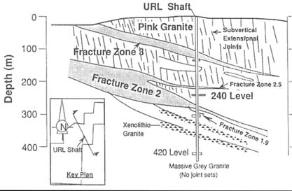
FIGURE 6.A1 Conceptual model of the rock mass at the Underground Research Laboratory (URL) in Manitoba, Canada. From Davison et al. (1993).
Based on knowledge gained from the site investigation, a model of groundwater flow was constructed. The model treated the fracture zones as discrete features and the rock mass away from the fracture zones as a porous medium. Two models were constructed at different scales. A regional-scale model was developed to define boundary conditions for a local-scale model. The regional-scale model was calibrated by adjusting recharge until the water table coincided with the land surface. The local-scale model was calibrated by adjusting parameters in fracture zones until calculated drawdowns agreed with measured drawdowns from hydraulic tests. After calibration, the local-scale model was used to predict drawdown at 171 packer-isolated intervals in the borehole monitoring network and the rate of seepage into the shaft during construction.
The URL model was relatively effective in predicting drawdown during shaft construction. Much of the success resulted from the effectiveness of site characterization prior to model development. The single most important aspect of this characterization was identification of the major geological features (the subhorizontal fracture zones) controlling flow at the site. For most of the 171 measurement locations, the magnitude and temporal variation of the drawdown were predicted to within an order of magnitude. Discrepancies between model predictions and field measurements were inversely proportional to the radial distance from the shaft; smaller discrepancies occurred at greater distances from the shaft. However, the onset of significantly measured drawdown consistently occurred 20 to 30 days earlier than predicted. This was attributed to differences
between assumed and actual shaft deepening rates, as well as the existence of extensive permeable vertical fractures providing good hydraulic communication between fracture zone 3 and the rock some 70 to 80 m above and below the zone. This situation was not detected during any of the site characterization activities carried out prior to excavation. The predicted inflow rate was approximately four times the measured rate (Figure 6.A2). This difference can be attributed in part to a combination of local effects related to the fine-scale distribution of fractures adjacent to the shaft.
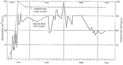
FIGURE 6.A2 Comparison of observed and predicted drawdown using a continuum model for the URL drawdown experiment. The measured inflow is plotted on the left-hand scale, and the predicted inflow on the right-hand scale. From Davision et al. (1987).
APPENDIX 6. B
PERCOLATION THEORY
Percolation theory is the study of random networks of conductors. The simplest example of a percolation network, a simple lattice percolation, can be constructed by creating a lattice of conductors and randomly turning some of them off. Examples of square lattices are shown in the top row of Figure 6.B1. Here, each of the conductors in the square lattice is left on with probability p (0 ≤ p ≤ 1) and turned off with probability 1 - p. The on-off decisions are statistically independent. The fundamental parameter that describes the statistical model for percolation in this case is p. One example of a percolation network applicable to fracture models is continuum percolation, where sets of conductors are placed randomly in space and overlapping conductors are connected. An example of a continuum percolation network is illustrated in the bottom row of Figure 6.B1.
Usually percolation networks are studied using numerical simulations of finite-sized domains (Zallen, 1983). Some analytical results for infinite-sized percolation networks also are known (Kesten, 1987). These results suggest that percolation models have two basic properties. The first is the existence of a critical density of conductors. Below the critical density there are only finite-sized clusters of connected conductors (no percolation), and above the critical density there is an infinite cluster (or clusters) of connected fractures (percolation). For large, finite-sized percolation models, this means that there is a high probability that no clusters span the largest length scale when the density is below the critical value. Conversely, there is a high probability that a cluster will span the
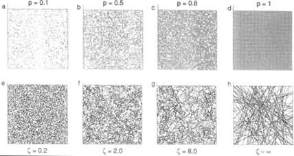
FIGURE 6.B1 Examples of fracture networks with different degrees of connectivity. Parts (a)–(d) are regular lattices that correspond to the random Poisson networks; (e)–(h) shown below them.
largest length scale when the density is above the critical value. For simple lattice percolation the critical density corresponds to a value for p called pc. In the continuum percolation case the controlling parameters are the spatial density, size, and orientation of the random sets. In some cases one can find a way to map the parameters of the continuum percolation model into an effective p and then apply the results predicted by simple lattice percolation (Hestir and Long, 1990).
The second basic property of percolation networks is that universal scaling laws appear when the fracture density is near the critical value. To explain this, suppose p is near pc and M represents a particular physical property of the percolation network, such as average permeability. Then M will be related to p in the following way:
where the exponent ![]() is referred to as a universal scaling exponent. The term universal is used because numerical studies suggest that the exponent depends only on the dimension of the percolation model (e.g., two or three dimensions) and not the details of the model, such as the kind of lattice used or the types of random sets in the continuum percolation case.
is referred to as a universal scaling exponent. The term universal is used because numerical studies suggest that the exponent depends only on the dimension of the percolation model (e.g., two or three dimensions) and not the details of the model, such as the kind of lattice used or the types of random sets in the continuum percolation case.
It is reasonable to suggest that most random network models will have two basic properties: critical density and scaling laws with universal exponents. Hence, these properties are also expected to apply in the case of a network of fractures. However, there is no general way to apply these concepts in a field situation, so percolation theory can only be used as a general framework for thinking about fracture and fluid flow problems. For some example applications of percolation theory to flow in a single fracture, see Chapter 3.
APPENDIX 6.C
CONNECTIVITY
A flow system with many fractures can have a high or low permeability depending on the connectivity of the fracture network (Figure 6.B1). Although the term connectivity has no generally accepted definition, it is normally used to describe the subjective appearance of a fracture network. Highly connected networks are more permeable. In some cases, where there is a specific mathematical model for the fractures, connectivity can be rigorously defined.
One of the best-known cases where connectivity has been studied is the percolation model. As noted in Appendix 6.B on percolation theory, percolation networks are constructed by creating a lattice of conductors and randomly turning some of them off. Several quantities can be defined that describe connectivity in percolation networks; each is based on assigning an arbitrary point on the lattice to be the origin. Connectivity measures include (1) the expected number of conductors connected to the origin, and (2) the probability that there is a path from the origin to a point x in the lattice. This latter probability is called the connectivity function. The higher the expected number of conductors, or the greater the probability of a path between the origin and point x, the greater the connectivity, ![]() .
.
A model that is similar to percolation networks is the continuum percolation model. One method for quantifying connectivity in these models involves choosing an arbitrary fracture and labeling it level one (Billaux et al., 1989). The fractures intersecting the level one fracture are then counted and labeled as level two fractures. Next, the number of fractures intersecting level two fractures that were not previously labeled are counted and labeled as level three fractures, and so on. The connectivity measure is given by a count of the number of fractures at each level; more connected systems have an increasing number of fractures at each level, whereas less connected systems have fewer fractures or no fractures at each level.
A third measure of connectivity is the average number of intersections per fracture (Figure 6.B1). This measure was used by Robinson (1984) and Long and Hestir (1990) for Poisson line systems. In this simplified system an analytical expression can be derived for the average number of intersections per fracture. This number is then taken to be the connectivity measure. In this case the permeability of the network is a definable function of connectivity.
Except for the Poisson line model, the other measures of connectivity described above have no known analytical description but can only be determined by numerical methods. To the extent that fracture systems can be reduced to statistical models characterizing the hydraulically active fracture system, the geometric analysis of connectivity will be indicative of permeability.
REFERENCES
Acuna, J. A., and Y. C. Yortsos. 1991. Numerical construction and flow simulation in networks of fractures using fractal geometry. Paper SPE-22703 presented at the 66th Annual Technical Conference, Society of Petroleum Engineers, Dallas, Oct. 6-9.
Anderson, J., and R. Thunvik. 1986. Predicting mass transport in discrete fracture networks with the aid of geometrical field data, Water Resources Research, 22(13):1941–1950.
Aviles, C. A., C. H. Scholz, and J. Boatwright. 1987. Fractal analysis applied to characteristic segments of the San Andreas fault. Journal of Geophysical Research, 92:331–344.
Bachu, S., ed. 1990. Parameter identification and estimation for aquifer and reservoir characterization. In Proceedings, 5th Canadian/American Conference on Hydrogeology, Calgary, Alberta, Canada, September 18-20. Dublin, Ohio: National Water Well Association.
Baecher, G. B. 1972. Site exploration: A probabilistic approach. Ph.D. thesis, Department of Civil Engineering, Massachusetts Institute of Technology, Cambridge.
Baecher, G. B., N. A. Lanney, and H. H. Einstein. 1977. Statistical description of rock properties and sampling. Pp. 5C1–5C8 in Proceedings, 18th United States Symposium on Rock Mechanics, Colorado School of Mines. Golden, Colo.: Johnson Publishing Co.
Barker, J. 1988. A generalized radial flow model for pumping tests in fractured rock. Water Resources Research, 24(10):1796–1804.
Barnsely, M. 1988. Fractals Everywhere. San Diego, Calif.: Academic Press, 396 pp.
Barton, C. C. 1995. Fractal analysis of the scaling and spatial clustering of fractures. In Fractals and Their Use in Earth Sciences, C. C. Barton and P. R. LaPointe, eds. New York: Plenum Publishing Co.
Barton, C. C., and P. A. Hsieh. 1989. Physical and Hydrologic-Flow Properties of Fractures. Field Trip Guidebook T385. Washington, D.C.: American Geophysical Union.
Barton, C. C., and E. Larsen. 1985. Fractal geometry of two-dimensional fracture networks at Yucca Mountain, Southwestern Nevada. Proceedings, International Symposium on Fundamentals of Rock Joints. Bjorkliden, Sweden: Centek Publishers.
Barton, C. M. 1978. Analysis of joint traces. Pp. 38–41 in Proceedings of the 19th U.S. Symposium on Rock Mechanics. Reno, Nev.: Conferences and Institutes.
Bear, J., C. F. Tsang, and G. de Marsily. 1993. Flow and Contaminant Transport in Fractured Rock . New York: Academic Press.
Berkowitz, B., and I. Balberg. 1993. Percolation theory and its applications to groundwater hydrology. Water Resources Research, 29(4):775–794.
Beveye, P., and G. Sposito. 1984. The operational significance of the continuum hypothesis in the theory of water movement through soils and aquifers. Water Resources Research, 20:521–530.
Beveye, P., and G. Sposito. 1985. Macroscopic balance equations in soils and aquifers: the case of space and time-dependent instrumental response. Water Resources Research, 21(8):1116–1120.
Billaux, D., J. P. Chiles, K. Hestir, and J. C. S. Long. 1989. Three-dimensional statistical modeling of a fractured rock mass—an example from the Fanay-Augeres Mine. International Journal of Rock Mechanics and Mining Science and Geomechanical Abstracts, 26(3/4):281–299.
Black, J. H., O. Olsson, J. E. Gale, and D. C. Holmes. 1991. Characterization and validation Stage 4: preliminary assessment and detail predictions. TR 91-108, Swedish Nuclear Power and Waste Management Co., Stockholm.
Bodvarrson, G. S., and P. A. Witherspoon. 1989. Geothermal reservoir engineering, Part 1 . Geothermal Science and Technology, 2(1):1–680.
Cacas, M. C., E. Ledoux, G. de Marsily, and B. Tillie. 1990. Modeling fracture flow with a stochastic discrete fracture network: calibration and validation. 1: The flow model. Water Resources Research, 26:479–489.
Carrera, J., J. Heredia, S. Vomvoris, and P. Hufschmied. 1990. Modeling of flow on a small fractured monzonitic gneiss block. Pp. 115–167 in Hydrogeology of Low Permeability Environments,
International Association of Hydrogeologists, Hydrogeology: Selected Papers, vol. 2, S. P. Neuman and I. Neretnieks, eds. Hannover: Heise.
Chang, J., and Y. C. Yortsos. 1990. Pressure transient analysis of fractal reservoirs. SPE Formation Evaluation, p. 631.
Childs, E. C. 1957. The anisotropic hydraulic conductivity of soil. Journal of Soil Science, 8(1):42–47.
Clemo, T. 1994. Dual permeability modeling of fractured media. Ph.D. thesis, University of British Columbia, Vancouver.
Conrad, F., and C. Jacquin. 1975. Representation of a two-dimensional fracture network by a probabilistic model: application to calculation of the geometric magnitudes of matrix blocks. UCRL-TRANS-10814. Translated from Revue de l'Institut Français du Pétrole, 28(6):843–890.
Cox, S. J. D., and L. Paterson. 1989. Tensile fracture of heterogeneous solids with distributed breaking strengths. Physical Review Board, 40:4690-4695.
Dagan, G. 1987. Theory of solute transport in water. Annual Reviews of Fluid Mechanics, 19:183–215.
Davison, C. C. 1985. URL Drawdown Experiment and comparison with models. TR 375, Atomic Energy of Canada Ltd., Pinawa, Manitoba.
Davison, C. C., T. Chan, and N. W. Scheier. 1987. Experimental activities of the Canadian nuclear fuel waste management program to validate geosphere models. Pp. 401–422 in Proceedings of GEOVAL-87: A Symposium on Verification and Validation of Geosphere Performance Assessment Models. Stockholm: Swedish Nuclear Power Inspectorate.
Davison, C. C., L. H. Frost, E. T. Kozak, N. W. Scheier, and C. D. Martin. 1993. Investigations of the groundwater transport characteristics of a large fracture zone in a granite batholith of different size scales. Pp. 331–338 in Proceedings of the 2d International Workshop on Scale Effects in Rock Masses, Scale Effects in Rock Masses 93, Pinto du Cusha, ed. Rotterdam: A. A. Balkema.
de Marsily, G. 1987. An overview of coupled processes with emphasis on geohydrology. Pp. 27–37 in Coupled Processes Associated with Nuclear Waste Repositories, C. F. Tsang, ed. New York: Academic Press.
Dershowitz, W. S. 1984. Rock joint systems, Ph.D. thesis, Massachusetts Institute of Technology, Cambridge.
Dershowitz, W. S., and H. H. Einstein. 1988. Characterizing rock joint geometry with joint system models. Rock Mechanics and Rock Engineering, 21:21–51.
Dershowitz, W., and I. Miller. 1995. Dual porosity fracture flow and transport. Geophysical Research Letters, 22(11):1441–1444.
Dershowitz, W., P. Wallmann, and S. Kindred. 1991a. Discrete Fracture Modeling for the Stripa Site Characterization and Validation Drift Inflow Predictions. SKB Report 91-16. Swedish Nuclear Power and Waste Management Co., Stockholm.
Dershowitz, W., P. Wallmann, J. E. Geier, and G. Lee. 1991b. Discrete Fracture Network Modeling of Tracer Migration Experiments at the SCV Site. SKB Report 91-23, Swedish Nuclear Power and Waste Management Co., Stockholm.
Doughty, C., J. C. S. Long, K. Hestir, and S. M. Benson. 1994. Hydrologic characterization of heterogeneous geologic media with an inverse method based on iterated function System. Water Resources Research, 30(6):1721-1745.
Duguid, J. O., and P. C. Y. Lee. 1977. Flow in fractured porous media. Water Resources Research, 13(3):558-566.
Dverstrop, B., and J. Anderson. 1989. Application of the discrete fracture network concept with field data: possibilities of model calibration and validation. Water Resources Research, 25(3):540-550.
Einstein, H. H., G. B. Baecher, and D. Veneziano. 1979. Risk analysis for rock slopes in open pit mines. Series of reports to U.S. Bureau of Mines. Pub. Nos. R80-17 to R80-22, Department of Civil Engineering, Massachusetts Institute of Technology, Cambridge.
Einstein, H. H., G. B. Baecher, and D. Veneziano, et al. 1980. Risk analysis for rock slopes in open pit mines—final technical report, Pub. No. R80-17, Department of Civil Engineering, Massachusetts Institute of Technology, Cambridge.
Einstein, H. H., D. Veneziano, G. B. Baecher, and K. J. O'Reilly. 1983. The effect of discontinuity persistence on rock slope stability. International Journal of Rock Mechanics and Mining Science and Geomechanics Abstracts , 20(5):227-236.
Elsworth, D. 1986. A model to evaluate the transient hydraulic response of three-dimensional, sparsely fractured rock masses. Water Resources Research, 22(13):1809-1819.
Endo, H. K. 1984. Mechanical transport in two-dimensional networks of fractures. Ph.D. thesis, University of California, Berkeley.
Endo, H. K., J. C. S. Long, C. K. Wilson, and P. A. Witherspoon. 1984. A model for investigating mechanical transport in fractured media. Water Resources Research, 20(10):1390-1400.
Evans, D. D., and T. J. Nicholson. 1987. Flow and Transport Through Unsaturated Fractured Rock. Monograph 42. Washington, D.C.: American Geophysical Union.
Freeze, R. A., and J. A. Cherry. 1979. Groundwater. Englewood Cliffs, N.J.: Prentice-Hall.
Freeze, R. A., J. W. Massmann, L. Smith, T. Sperling, and B. James. 1990. Hydrogeological decision analysis. 1: A framework. Groundwater, 28:738–766.
Geier, J. E., K. Lee, and W. S. Dershowitz. 1989. Field validation of conceptual models for fracture geometry. Unpublished monograph, Golder Associates, Redmond, Wash.
Gelhar, L. W., and C. L. Axness. 1983. Three-dimensional stochastic analysis of dispersion in aquifers. Water Resources Research, 19(1):161-1800.
Gilman, J.R., and H. Kazemi. 1983. Improvements in simulation of naturally fractured reservoirs. Society of Petroleum Engineers Journal, Aug.:695-707.
Glass, R. J., M. J. Nicholl, and V. C. Tidwell. 1995. Challenging models for flow in unsaturated, fractured rock through exploration of small scale processes. Geophysical Research Letters, 22(11):1457-1460.
Griffith, A. A. 1920. The phenomena of rupture and flow in solids. Royal Society (London) Philosophical Transactions series A, 221:163-198.
Herbert, A., and G. Lanyon. 1992. Modeling tracer transport in fractured rock at Stripa. SKB Report 92-01, Swedish Nuclear Power and Waste Management Co., Stockholm.
Herbert, A., J. Gale, G. Lanyon, and R. MacLeod. 1991. Modeling for the Stripa site characterization and validation drift inflow: prediction of flow through fractured rock. SKB Report 91-35. Swedish Nuclear Power and Waste Management Co., Stockholm.
Hestir, K., and J. C. S. Long. 1990. Analytical expressions for the permeability of random two-dimensional Poisson fracture networks based on regular lattice percolation and equivalent media theories. Journal of Geophysical Research, 95(B13):21565–21581.
Hirata, T. 1989. Fractal dimension of fault systems in Japan: fractal structure in rock fracture geometry at various scales. Pure and Applied Geophysics, 131:157-170.
Hsieh, P. A., and S. P. Neuman. 1985. Field determination of the three-dimensional hydraulic conductivity tensor of anisotropic media. 1. Theory. Water Resources Research, 21(11):1655–1666.
Hsieh, P. A., S. P. Neuman, G. K. Stiles, and E. S. Simpson. 1985. Field determination of the three-dimensional hydraulic conductivity tensor of anisotropic media. 2. Methodology and application to fractured rocks. Water Resources Research, 21(11):1667–1676.
Hudson, J. A., and P. R. La Pointe. 1980. Printed circuits for studying rock mass permeability. International Journal of Rock Mechanics and Mining Science and Geomechanics Abstracts, 17:297-301.
Hull, L., and T. Clemo. 1987. Section 4: Dual permeability model: Laboratory and FRACSL validation studies, in Geothermal Injection Technology Program Annual Progress Report Fiscal Year 1986. Idaho Falls, Idaho: Idaho National Engineering Lab.
Huyakorn, P. S., B. H. Lester, and C. R. Faust. 1983a. Finite element techniques for modeling groundwater flow in fractured aquifers. Water Resources Research, 19(4):1019-1035.
Huyakorn, P. S., B. H. Lester, and J. W. Mercer. 1983b. An efficient finite element technique for modeling transport in fractured porous media. 1: Single-species transport. Water Resources Research, 19(3):841-854.
Ibaraki, M. 1994. Colloid-facilitated contaminant transport in discretely-fractured porous media. Ph.D. thesis, University of Waterloo, Waterloo, Ontario, Canada.
Irmay, S. 1955. Flow of liquids through cracked media. Bulletin of the Water Resources Council, Israel, 5A(1):84.
Isaaks, E., and M. Srivastava. 1989. Applied Geostatistics. New York: Oxford University Press.
Iwai, K. 1976. Fundamental studies of fluid flow through a single fracture. Ph.D. dissertation, University of California, Berkeley.
Jones, J. W., E. S. Simpson, S. P. Neuman, and W. S. Keys. 1985. Field and theoretical investigations of fractured crystalline rock near Oracle, Arizona . CR-3736. Washington, D.C.: U.S. Nuclear Regulatory Commission.
Kazemi, H. 1969. Pressure transient analysis of naturally fractured reservoirs with uniform fracture distribution. Society of Petroleum Engineers Journal, 9:451-462.
Kazemi, H., and J. R. Gilman. 1993. Multiphase flow in fractured petroleum reservoirs. Pp. 267–323 in Flow and Contaminant Transport in Fractured Rocks, J. Bear, C. F. Tsang, and G. de Marsily, eds. New York: Academic Press.
Kesten, H. 1987. Percolation theory and first passage percolation. Annals of Probability, 15:1231–1271.
Khaleel, R. 1989. Scale dependence of continuum models for fractured basalts. Water Resources Research, 25(8):1847–1856.
Kirkpatrick, S., D. C. Gelatt, and M. P. Vecchi. 1983. Optimization by simulated annealing. Science, 220:671–680.
Kueper, B. H., and D. B. McWhorter. 1991. The behavior of dense non-aqueous phase liquids in fractured clay and rock. Groundwater, 29(5):716–725.
Kwicklis, E. D., and R. W. Healy. 1993. Numerical investigation of steady liquid water flow in a variably saturated fracture network. Water Resources Research, 29(12):4091–4102.
LaPointe, P. R. 1988. A method to characterize fracture density and connectivity through fractal geometry. International Journal of Rock Mechanics and Mining Science and Geomechanics Abstracts, 25:421–429.
LaPointe, P., and J. A. Hudson. 1985. Characterization and interpretation of rock mass joint patterns. Special Paper 199. Boulder, Colo.: Geological Society of America.
Lawn, B. R., and T. R. Wilshaw. 1975. Fracture of Brittle Solids. Cambridge: Cambridge University Press.
Lee, J. S., D. Veneziano, and H. H. Einstein. 1990. Hierarchical fracture trace model. In Proceedings of the 31st U.S. Symposium on Rock Mechanics. Rotterdam: A. A. Balkema.
Long, J. C. S. 1983a. Construction of equivalent discontinuum models for fracture hydrology. In J. A. Hudson, ed., Rock Testing and Site Characterization, vol. 3, Comprehensive Rock Engineering. New York: Pergamon Press.
Long, J. C. S. 1983b. Investigation of equivalent porous medium permeability in networks of discontinuous fractures. Ph.D. dissertation, University of California, Berkeley.
Long, J. C. S. 1993. Construction of equivalent discontinuum models for fracture hydrology, comprehensive rock engineering. J. Hudson, T. Brown, C. Fairhurst, and E. Hoek, eds. Oxford, N.Y.: Pergamon Press.
Long, J. C. S., and D. M. Billaux. 1987. From field data to fracture network modeling: an example incorporating spatial structure. Water Resources Research, 23(7):1201–1216.
Long, J. C. S., and K. Hestir. 1990. Permeability of random two-dimensional fracture networks. Journal of Geophysical Research, 95(B13):21,256.
Long, J. C. S., and P. A. Witherspoon. 1985. The relationship of the degree of interconnectivity to permeability in fracture networks. Journal of Geophysical Research, 90(B4):3087–3097.
Long, J. C. S., J. S. Remer, C. R. Wilson, and P. A. Witherspoon. 1982. Porous media equivalents for networks of discontinuous fractures. Water Resources Research, 18(3):645–658.
Long, J. C. S., P. Gilmour, and P. A. Witherspoon. 1985. A model for steady state flow in random, three-dimensional networks of disk-shaped fractures. Water Resources Research, 21(8):1150–1115.
Long, J. C. S., E. Majer, S. Martel, K. Karasaki, J. Peterson, Jr., A. Davey, and K. Hestir, 1990. Hydrologic characterization of fractured rocks—an interdisciplinary methodology. NAGRADOE Cooperative Project Report LBL-27863. Lawrence Berkeley Laboratory, Berkeley, Calif.
Long, J. C. S., C. Doughty, K. Hestir, and S. Martel. 1992a. Modeling heterogeneous and fractured reservoirs with inverse methods based on iterated function system. In Reservoir Characterization III, B. Linville, ed. Tulsa, Okla.: Pennwell Books.
Long, J. C. S., A. Mauldon, K. Nelson, S. Martel, P. Fuller, and K. Karasaki. 1992b. Prediction of flow and drawdown for the site characterization and validation site in the Stripa mine. SKB Report 92-05, Swedish Nuclear Power and Waste Management Co., Stockholm.
Long, J. C. S., O. Olsson, S. Martel, and J. Black. 1996. Effects of excavation on water inflow to a drift. In Fractured and Jointed Rock Masses. Rotterdam: A. A. Balkema.
Mardia, K. V. 1972. Statistics of Directional Data. San Diego: Academic Press.
Martel, S. J. 1992. Geologic characterization of fractures as aid to hydrologic modeling of the SCV block at the Stripa mine. Stripa Project Technical Report 92-24, Swedish Nuclear Power and Waste Management Co., Stockholm.
Martel, S. J., and J. E. Peterson, Jr. 1990. Use of integrated geologic and geophysical information for characterizing the structure of fracture systems at the US/UK site, Grimsel Laboratory, Switzerland. LBL-27912, Lawrence Berkeley Laboratory, Berkeley, Calif.
Martel, S. J., and J. E. Peterson. 1991. Interdisciplinary characterization of fracture systems at the US/BK site, Grimsel Laboratory, Switzerland. International Journal of Rock Mechanics and Mining Science and Geomechanics Abstracts, 28:259–323.
Martel, S. J., and J. E. Peterson. 1993. Techniques for assessing the in situ orientation distribution of fractures from borehole data. Geological Society of America Abstracts with Programs, 25(114).
Martel, S. J., D. D. Pollard, and P. Segall. 1988. Development of simple strike-slip fault zones in granitic rock, Mount Aboot quadrangle, Sierra Nevada, California. Geological Society of America Bulletin, 100:1451–1465.
Martel, S., K. Hestir, and J. C. S. Long. 1991. Generation of fracture patterns using self-similar iterated function concepts. 1990 Annual report, Earth Sciences Division, Lawrence Berkeley Laboratory, Berkeley, Calif., pp. 52–56.
McKay, L. D., R. W. Gillham, and J. A. Cherry. 1993. Field experiments in a fractured clay till. 2. Solute and colloid transport . Water Resources Research, 29(12):3879–3890.
Moench, A. F. 1984. Double porosity models for a fissured groundwater reservoir with fracture skin. Water Resources Research, 20(7):831–846.
Moreno, L., and I. Neretnieks. 1993. Flow and nuclide transport in fractured media: the importance of the flow-wetted surface for radionuclide migration. Journal of Contaminant Hydrology, 13:49–71.
National Research Council. 1990. Groundwater Models: Scientific and Regulatory Applications. Committee on Groundwater Modeling Assessment, Water Science and Technology Board. Washington, D.C.: National Academy Press.
Neuman, S. P. 1987. Stochastic continuum representation of fractured rock permeability as an alternative to the REV and fracture network concepts. Pp. 533–561 in Rock Mechanics, Proceedings of the 28th U.S. Rock Mechanics Symposium. Rotterdam: A. A. Balkema.
Neuman, S. P. 1990. Universal scaling of hydraulic conductivities and dispersivities in geologic media. Water Resources Research, 26(8):1749–1758.
Neuman, S. P. 1994. Generalized scaling of permeability values: validation and effect of support scale. Geophysical Research Letters, 21(5):349–352.
Neuman, S. P., and J. S. Depner. 1988. Use of variable scale pressure test data to estimate the log hydraulic conductivity covariance and dispersivity of fractured granites near Oracle, Arizona . Journal of Hydrology, 102(1–4):475–501.
Neuman, S. P., and S. Orr. 1993. Prediction of steady-state flow in non uniform geologic media by conditional moments: exact non local formalism, effective conductivities, and weak approximation. Water Resources Research, 29(2):341–364.
Neuman, S. P., E. S. Simpson, P. A. Hsieh, J. W. Jones, and C. L. Winter. 1985. Statistical analysis of hydraulic test data from crystalline rock near Oracle, Arizona. International Association of Hydrogeologists, Memoires, vol. XVII.
Nordqvist, A. W., Y. W. Tsang, C. F. Tsang, B. Dverstrop, and J. Anderson. 1992. A variable aperture fracture network model for flow and transport in fractured rocks. Water Resources Research, 28(6):1703–1714.
Oda, M. 1985. Permeability tensor for discontinuous rock masses. Geotechnique, 35(4):483–495.
Oda, M., Y. Hatsuyama, and Y. Ohnishi. 1987. Numerical experiments on permeability tensor and its application to jointed granite at Stripa mine, Sweden. Journal of Geophysical Research, 92(B8):8037–8048.
Odling, N. E., and I. Webman. 1991. A conductance mesh approach to the permeability of natural and simulated fracture patterns. Water Resources Research, 27:2633–2644.
Okubo, P. G., and K. Aki. 1987. Fractal geometry in the San Andreas fault system. Journal of Geophysical Research, 92:345–355.
Okusu, N. M., K. Karasalai, J. C. S. Long, and G. Bodvarsson. 1989. FMMG: a program for discretizing two-dimensional fracture matrix systems. Theory, design, and user's manual. LBL-26 782, Lawrence Berkeley Laboratory, Berkeley, Calif.
Olson, J. 1991. Fracture mechanics analysis of joints and veins. Ph.D. dissertation, Stanford University, Stanford, Calif.
Olsson, O., ed. 1992. Site characterization and validation. Final Report, Stripa Project, 92-22, Conterra AB, Uppsala, Sweden.
Orbach, R. 1986. Dynamics of fractal networks. Science, 231:814–819.
Parney, R., and L. Smith. 1995. Fluid velocity and path length in fractured media. Geophysical Research Letters, 22(11):1437–1440.
Persoff, P., K. Pruess, and L. Myer. 1991. Two-phase flow visualization and relative permeability measurement in transparent replicas of rough-walled rock fractures . In Proceedings of the 16th Workshop on Geothermal Reservoir Engineering. Stanford, Calif.: Stanford University.
Peters, R. R., and E. A. Klavetter. 1988. A continuum model for water movement in unsaturated fractured rocks. Water Resources Research, 24(3):416–430.
Pollard, D. D., and A. Aydin. 1988. Progress in understanding jointing over the past century. Geological Society of America Bulletin, 100:1181–1204.
Pollek, J. M. 1990. Studies of the hydraulic behavior of hierarchically fractured geometries. LBL-28612, Lawrence Berkeley Laboratory, Berkeley, Calif., 72 pp.
Power, W. L., and T. E. Tullis. 1991. Euclidian and fractal models of surface roughness. Journal of Geophysical Research, 96:415–424.
Power, W. L., T. E. Tullis, S. R. Brown, G. N. Boitnott, and C. H. Scholz. 1987. Roughness of natural fault surfaces. Geophysical Research Letters, 14:29–32.
Priest, S. D., and J. Hudson. 1976. Discontinuity spacings in rock. International Journal of Rock Mechanics and Mining Science, 13:135–148.
Pruess, K., and K. Karasaki. 1982. Proximity functions for modeling fluid and heat flow in reservoirs with stochastic fracture distributions. In Proceedings of the 8th Workshop on Geothermal Reservoir Engineering. Stanford, Calif.: Stanford University.
Pruess, K., and T. N. Narasimhan. 1988. Numerical modeling of multiphase and nonisothermal flows in fractured media. In Proceedings of the Symposium Conference on Fluid Flow in Fractured Rocks, Georgia State University, May 15-18.
Pruess, K., and J. S. Y. Wang. 1987. Numerical modeling of isothermal and nonisothermal flow in unsaturated fractured rock—A review. Pp. 11–21 in Flow and Transport Through Unsaturated
Fractured Rocks, D. D. Evans, and T. J. Nicholson, eds., Monograph 42. Washington, D.C.: American Geophysical Union.
Rasmussen, T. C. 1991. Steady fluid flow and travel times in partially saturated fractures using a discrete air-water interface. Water Resources Research, 27(1):67.
Rasmussen, T. C., and D. P. Evans. 1993. Water infiltration into exposed fractured rock surfaces. Soil Science Society Journal, 57(2):324–329.
Reeves, M., G. A. Freeze, V. A. Kellel, J. F. Pickens, D. T. Upton, and P. B. Davies. 1991. Regional double porosity solute transport in the Culebra dolomite under brine-reservoir-breach release conditions: an analysis of parameter sensitivity and importance. SAND89–7069, Sandia National Laboratories, Albuquerque, N.M.
Robinson, P. 1984. Connectivity, flow and transport in network models of fractured media. Ph.D. thesis, Oxford University.
Rouleau, A. 1984. Statistical characterization and a numerical simulation of a fracture system—application to groundwater flow in the Stripa granite. Ph.D. thesis, University of Waterloo, Waterloo, Ontario, Canada.
Scholz, C. H., and C. A. Aviles. 1986. The fractal geometry of faults and faulting. Pp. 145–155 in Earthquake Source Mechanics, S. Das, J. Boatwright, and C. H. Scholz, eds. Geophysical Monograph Series, vol. 37. Washington, D.C.: American Geophysical Union.
Schwartz, F. W., and L. Smith. 1988. A continuum approach for modeling mass transport in fractured media. Water Resources Research, 24(8):1360–1372.
Segall, P., and D. D. Pollard. 1989. Joint formation in granitic rock of the Sierra Nevada. Geological Society of America Bulletin, 94:563–575.
Segan, S., and K. Karasaki. 1993. TRINET: a flow and transport code for fracture networks—user's manual and tutorial. LBL-34834, Lawrence Berkeley Laboratory, Berkeley, Calif.
Shapiro, A. M., and J. Anderson. 1985. Simulation of steady state flow in three-dimensional fracture networks using the boundary element method. Advances in Water Research, 8(3).
Shimo, M., and J. C. S. Long. 1987. A numerical study of transport parameters in fracture networks. In Flow and Transport Through Unsaturated Fractured Rocks, D. D. Evans and T. J. Nicholson, eds. Monograph 42. Washington, D.C.: American Geophysical Union.
Smith, L., and F. W. Schwartz. 1984. An analysis of the influence of fracture geometry on mass transport in fractured media. Water Resources Research, 20(9):1241–1252.
Smith, L., and F. W. Schwartz. 1993. Solute transport through fracture networks. In Flow and Contaminant Transport in Fractured Rocks, J. Bear, C. F. Tsang, and G. de Marsily, eds. New York: Academic Press.
Smith, L., T. Clemo, and M. Robertson. 1990. New approaches to the simulation of field scale solute transport in fractured rocks. In Proceedings of the 5th Canadian/American Conference on Hydrogeology, S. Bachu, ed. Dublin, Oh.: National Waterwell Association.
Smith, L., C. W. Mase, F. W. Schwartz, and D. Chorley. 1985. Dispersion in three-dimensional fracture networks. In Hydrogeology of Rocks of Low Permeability Symposium. Tucson, Ariz.: International Association of Hydrogeologists.
Snow, D. 1965. A parallel-plate model of fractured permeable media. Ph.D. dissertation, University of California, Berkeley.
Sudicky, E. A., and R. G. McLaren. 1992. The Laplace transform Galerkin technique for large scale simulation of mass transport in discretely fractured porous formations. Water Resources Research, 28(2):499–514.
Takayasu, H. 1985. A deterministic model of fracture. Progress in Theoretical Physics, 74:1343–1345.
Tchalenko, J. S. 1970. Similarities between shear zones of different magnitudes. Geological Society of America Bulletin, 81:1625–1640.
Termonia, Y., and P. Meakin. 1986. Formation of fractal cracks in a kinetic fractal model. Nature, 320:429–431.
Terzaghi, R. 1965. Sources of errors in joint surveys. Geotechnique, 15:287–303.
Teufel, L. W., D. W. Rhett, and H. E. Farrell. 1991. Effects of reservoir depletion and pore pressure drawdown on in-situ stress and deformation in Ekofisk Field, North Sea. Pp. 63–72 in Proceedings of the 32nd U.S. Rock Mechanics Symposium . Rotterdam: A. A. Balkema.
Therrien, R. 1992. Three-dimensional analysis of variably-saturated flow and solute transport in discretely-fractured porous media. Ph.D. dissertation, University of Waterloo, Waterloo, Ontario, Canada.
Vandergraaf, T. T. 1995. Radionuclide migration experiments under laboratory conditions. Geophysical Research Letters, 22(11):1409–1412.
Veneziano, D. 1978. Probabilistic modeling of joints in rock. Unpublished manuscript, Massachusetts Institute of Technology, Cambridge.
Wang, J. S. Y., and T. N. Narasimhan. 1985. Hydrologic mechanisms governing fluid flow in a partially saturated, fractured porous medium. Water Resources Research, 20(12):1861–1874.
Warburton, P. M. 1980a. A stereological interpretation of joint trace data. International Journal of Rock Mechanics and Mining Sciences, 17:181–190.
Warburton, P. M. 1980b. A stereological interpretation of joint trace data: influence of joint shape and implications for geological surveys. International Journal of Rock Mechanics and Mining Sciences, 17:305–316.
Warren, J. E., and P. J. Root. 1963. The behavior of naturally fractured reservoirs. Society of Petroleum Engineers Journal, 3:245–255.
Wels, C., and L. Smith. 1994. Retardation of sorbing solutes in fractured media. Water Resources Research, 30(9):2547–2563.
Zallen, R. 1983. Physics of Amorphous Solids. New York: John Wiley.


