
Page 125
5
Statistical Issues
In Chapter 4, we presented ways to estimate the frequencies of genotypes and profiles in the population. In this chapter, we consider how to interpret frequencies as probabilities and likelihood ratios and how to make adjustments when a suspect is found through a database search. We also discuss the degree of uncertainty of such estimates according to statistical theory and empirical tests that use different databases. Finally, we ask how many loci would be needed to establish a profile as unique. The chapter includes a discussion of the statistics of matching and binning of VNTRs.1
Two major issues regarding uncertainty must be addressed in the statistical evaluation of DNA evidence. One is associated with the characteristics of a database, such as its size and whether it is representative of the appropriate population. The other might be called the subpopulation problem. In the first instance, inferences based on values in a database might be uncertain because the database is not compiled from a sample of the most relevant population or the sample is not representative. If the database is small, the values derived from it can be uncertain even if it is compiled from a scientifically drawn sample; this can be addressed by providing confidence intervals on the estimates. The second issue, the subpopulation problem, is broader than the first. Although the formulae might provide good estimates of the match probability for the average member of the population, they might not be appropriate for a member of an unusual
1 Some references for general background that are pertinent to this chapter or parts of it are Aldous (1989), Finkelstein and Levin (1990), Aitken and Stoney (1991), Aitken (1995).
Page 126
subgroup. Our approach is empirical: we compare different subpopulations and also, to mimic a worst case scenario, perform sample calculations deliberately using an inappropriate database.
Data Sources
A simple random sample of a given size from a population is one chosen so that each possible sample has an equal chance of being selected. Ideally, the reference data set from which genotype frequencies are calculated would be a simple random sample or a stratified or otherwise scientifically structured random sample from the relevant population. Several conditions make the actual situation less than ideal. One is a lack of agreement as to what the relevant population is (should it be the whole population or only young males? should it be local or national?) and the consequent need to consider several possibilities. A second is that we are forced to rely on convenience samples, chosen not at random but because of availability or cost. It is difficult, expensive, and impractical to arrange a statistically valid random-sampling scheme. The saving point is that the features in which we are interested are believed theoretically and found empirically to be essentially uncorrelated with the means by which samples are chosen. Comparison of estimated profile frequencies from different data sets shows relative insensitivity to the source of the data, as we document later in the chapter. Furthermore, the VNTRs and STRs used in forensic analysis are usually not associated with any known function and therefore should not be correlated with occupation or behavior. So those convenience samples are effectively random.
The convenience samples from which the databases are derived come from various sources. Some data come from blood banks. Some come from genetic-counseling and disease-screening centers. Others come from mothers and putative fathers in paternity tests. The data summarized in FBI (1993b), which we have used in previous chapters and will again in this chapter, are from a variety of sources around the world, from blood banks, paternity-testing centers, molecular-biology and human-genetics laboratories, hospitals and clinics, law-enforcement officers, and criminal records.
As mentioned previously, most markers used for DNA analysis, VNTRs and STRs in particular, are from regions of DNA that have no known function. They are not related in any obvious way to gene-determined traits2, and there is no reason to suspect that persons who contribute to blood banks or who have been
2 Some loci used in PCR-based typing are associated with genes. It is important to determine if a particular forensic allele is associated with a disease state and hence subject to selection. A forensic marker might happen to be closely linked to an important gene, such as one causing some observable trait, and could conceivably be in strong linkage disequilibrium. As the number of mapped genes increases, this will become increasingly common. But for that to affect the reliability of a database, the trait would have to appear disproportionately in the populations that contribute to the database.
Page 127
involved in paternity suits or criminal proceedings differ from a random sample of the population with respect to DNA markers. In addition, there is empirical evidence to the contrary: If we compare samples chosen in different ways, the results from calculations made from the different databases are quite similar.
Although most of the data that we are concerned with are from persons in the United States, there are increasing numbers from elsewhere in the world, and these can be used for comparison. The 1993 FBI compendium includes samples from whites in the United States (Arizona, California, Florida, Georgia, Illinois, Kentucky, Maryland, Michigan, Minnesota, Missouri, Nevada, North Carolina, Oregon, South Carolina, Vermont, Virginia, and Washington), France, Israel, Spain, Switzerland, Denmark, England, Germany, Finland, Italy, and Tasmania. Data on blacks come from the United States (California, Florida, Georgia, Kentucky, Maryland, Michigan, Minnesota, Nevada, North Carolina, Oregon, South Carolina, Virginia, and Washington), Haiti, Togo, and England. Data on Hispanics come from several states in the United States. The FBI places data from eastern and western US Hispanics into separate databases because of the somewhat different origins of these populations.
American Indians present a special difficulty because they have more population subdivision, as demonstrated by higher values of ![]() (see Chapter 4), than populations of whites, blacks, or Hispanics. The data are increasing rapidly, and substantial numbers are available from Arizona, Minnesota, North Carolina, Oregon, Ontario, and Saskatchewan, as well as from particular tribes (Sioux, Navaho).
(see Chapter 4), than populations of whites, blacks, or Hispanics. The data are increasing rapidly, and substantial numbers are available from Arizona, Minnesota, North Carolina, Oregon, Ontario, and Saskatchewan, as well as from particular tribes (Sioux, Navaho).
Match Probability and Likelihood Ratio
Suppose that a DNA sample from a crime scene and one from a suspect are compared, and the two profiles match at every locus tested. Either the suspect left the DNA or someone else did. We want to evaluate the probability of finding this profile in the "someone else" case. That person is assumed to be a random member of the population of possible suspects. So we calculate the frequency of the profile in the most relevant population or populations. The frequency can be called the random-match probability, and it can be regarded as an estimate of the answer to the question: What is the probability that a person other than the suspect, randomly selected from the population, will have this profile? The smaller that probability, the greater the likelihood that the two DNA samples came from the same person. Alternatively stated, if the probability is very small, we can say that either the two samples came from the same person or a very unlikely coincidence has occurred. (As in Chapter 4, the calculations in this chapter assume that no error has occurred in the determination of the DNA profiles.)
An alternative is to calculate the likelihood ratio (LR), a measure of the strength of the evidence regarding the hypothesis that the two profiles came from
Page 128
the same source. Suppose we find that the profiles of the person contributing the evidence DNA (E) and of the suspect (S) are both x. We consider two hypotheses: (1) the source of the evidence and the suspect are the same person, (2) the source of the evidence is a randomly selected person unrelated to the suspect. Although there are other possible hypotheses, it is usually sufficient to consider only these two. The likelihood ratio is the probability under hypothesis (1) that the suspect profile and the evidence-sample profile will both be x, divided by the corresponding probability under hypothesis (2). The greater the likelihood ratio, the stronger is the evidence in favor of the hypothesis corresponding to the numerator, that the source of the evidence-sample DNA and the suspect are the same person.
To write that symbolically, we let Pr1 and Pr2 indicate probabilities calculated under hypotheses 1 and 2. The LR for this simple comparison is
![]() (5.1a)
(5.1a)
Using a vertical line to indicate conditioning (statements to the left of the vertical line are conditional on statements to the right; for example, ![]() is the probability that the evidence sample will have profile x given that the suspect has profile x), we note that
is the probability that the evidence sample will have profile x given that the suspect has profile x), we note that
![]()
We can then rewrite Equation 5.1a in two algebraically equivalent forms:
![]() (5.1b)
(5.1b)
![]() (5.1c)
(5.1c)
Unless an error has occurred in the DNA typing, the numerator in Equations 5.1b and 5.1c will always equal one if the profiles match. Suppose that the population frequency of x is P(x), and assume that the persons who contributed E and S, if different, are unrelated (and E and S are therefore statistically independent). Then the denominator is P(x), so
![]() (5.2)
(5.2)
Therefore, in the usual case, the likelihood ratio is the reciprocal of the probability of a random match.3
The likelihood ratio, then, is a way of summarizing the DNA evidence. If
3 Under some circumstances, such as if the match window is small, the probability of a match between two samples from the same person might be less than 1. In principle, this could change the likelihood ratio (Kaye 1995b); in practice, the possible error is minuscule in comparison with uncertainties in the denominator. The effect of the size of the match window on the probability of a false negative is discussed later in the chapter.
Page 129
the LR is 1,000, the probability that the profiles are the same is 1,000 times as great if the samples came from the same person as it is if they came from different persons.
In the situation described above and reflected in the notation E and S, we imagine an evidence sample left at the crime scene by the putative perpetrator and a suspect with a matching profile. Although that is conceptually the simplest scenario and is used throughout this report for illustrative purposes, the mathematical formalism is valid more generally. For example, if a suspect is apprehended with blood on his clothes, this blood is the evidence sample to be matched against the genotypic profile of the victim. The LR given above is still valid, although for the most direct interpretation one would use Equation 5.1b, with S denoting the profile of the victim and E the evidence-sample profile.
Mixed Samples
Mixed samples are sometimes found in crime situations—for instance, blood from two or more persons at the scene of a crime, victim and assailant samples on a vaginal swab, and material from multiple sexual assailants. In many cases, one of the contributors—for example, the victim—is known, and the genetic profile of the unknown is readily inferred. In some cases, it might be possible to distinguish the genetic profiles of the contributors to a mixture from differences in intensities of bands in an RFLP pattern or dots in a dot-blot typing; in either case, the analysis is similar to the unmixed case. However, when the contributors to a mixture are not known or cannot otherwise be distinguished, a likelihood-ratio approach offers a clear advantage and is particularly suitable.
Consider a simple case of a VNTR analysis in which, for a particular locus, there are four bands in the lane, known to be contributed by two persons. If the alleles from the two persons are known and correspond to the set of four in the lane, there is usually no problem of interpretation, since two of the bands will match one suspect and the other two bands will match the other. However, two of the bands might match the alleles of only one suspect, and the source of the other two might be unknown. The 1992 report (NRC 1992, p 59) says: "If a suspect's pattern is found within the mixed pattern, the appropriate frequency to assign such a 'match' is the sum of the frequencies of all genotypes that are contained within (i.e., that are a subset of) the mixed pattern." Suppose the four bands correspond to alleles (bins) A1, A2, A3, and A4, whose frequencies are p1. p2, p3, and p4. This procedure recommended in the 1992 report would calculate the match probability as
![]()
that is, the probability that a randomly selected person would have two alleles from the set of possibilities (A1, A2, A3, A4). As above, the reciprocal of this probability can be interpreted as a likelihood ratio.
Page 130
That calculation is hard to justify, because it does not make use of some of the information available, namely, the genotype of the suspect. The correct procedure, we believe, was described by Evett et al. (1991). Suppose that the suspect's genotype is A1A2. The hypothesis we wish to test is that the samples came from the suspect and one other person. The probability under this hypothesis of finding the profile shown by the evidence sample is 2p3p4, because under this hypothesis it is certain that two of the bands are A1 and A2. If the samples came from two randomly selected persons, the probability of any particular pair of profiles, such as A1A3 and A2A4, is (2p1p3)(2p2p4) = 4P1P2P3P4. There are six possible pairs of two-band profiles corresponding to the four bands, so the total probability is 24p1p2p3p4. The likelihood ratio, analogous to Equations 5.1, is
![]()
This LR, compared with that derived from the recommendation of the 1992 NRC report, is larger when the suspect bands are relatively rare and smaller when the suspect bands are relatively common. The reason is that we have taken account of the information in the genotype of the suspect rather than averaging over the set of possible genotypes consistent with the four-band evidence-sample profile.
There might be fewer than four bands, or multiple suspects might be identified. These and other, more complex cases can be analyzed in a similar manner (Evett et al. 1991). Some cases are treated in Appendix 5A and summarized in Table 5.1.
We have considered only simple cases. With VNTRs, it is possible, though very unlikely, that the four bands were contributed by more than two persons, who either were homozygous or shared rare alleles. With multiple loci, it will usually be evident if the sample was contributed by more than two persons. Calculations taking those possibilities into account could be made if there were reason to believe that more than two persons contributed to the sample.
Mixed samples are often difficult to analyze in systems where several loci are analyzed at once. Mixed samples can also lead to more complicated calculations with DQA, where some alleles are inferred by subtraction. (For example, there is no specific probe for the allele 1.2; the presence or absence of this allele is inferred from the reaction of DNA probes with the product of the combination 1.2, 1.3, and 4, but not with the products of 1.3 and 4 individually.)
The problem is complex, and some forensic experts follow the practice of making several reasonable assumptions and then using the calculation that is most conservative. For a fuller treatment of mixed samples, see Weir et al. ( 1996).
Bayes's Theorem
The likelihood ratio and the match probability, being reciprocals, contain the same information. The LR, however, has a property that makes it especially
Page 131
useful, provided that prior odds are available on the hypothesis that the two DNA profiles have the same source. (Prior odds are the odds that the two DNA samples came from the same person on the basis of information other than the DNA. Posterior odds are the odds when the DNA information is included in the analysis.) That property can be stated this way:
The posterior odds are the prior odds multiplied by LR.4
In everyday words: Whatever are the odds that the two samples came from the same person in the absence of DNA evidence, the odds when the DNA evidence is included are LR times as great. That statement is an instance of Bayes's theorem.
For example, if there is reason to think that the prior odds that two DNA samples came from the same person (however this is determined) are 1:2, and the LR is 10,000, the posterior odds are 5,000:1. Many statisticians and forensic scientists prefer to use the likelihood ratio rather than the match probability (Berry 1991a; Berry et al. 1992; Evett et al. 1992; Balding and Nichols 1994; Collins and Morton 1994) because it admits an inferential interpretation that the simple match probability does not. Odds can be converted into a probability by the relation Prob = Odds/(Odds + 1), or Odds = Prob/(1-Prob). Thus, a likelihood ratio, which is not a probability, can be used to obtain a probability.
Paternity testing
The relation between posterior and prior odds is routinely used in paternity analysis (Walker 1983; AABB 1994). If the putative father is not excluded by blood-group, enzyme, and DNA evidence, a ''paternity index" is calculated. The paternity index PI is a likelihood ratio—the probability of the mother-child-father profile combination if the putative father is the true father divided by the probability of this combination if a randomly selected man is the father. Customarily, the calculations make use of a database or databases appropriate to the race(s) of the persons involved.
If the prior odds are 1:1—that is, if the putative father is assumed to be equally likely to be and not to be the true father—the posterior odds are the same as the likelihood ratio; but for other prior odds, that is not the case. Suppose that PI is calculated to be 1,000. If the prior odds (from evidence other than that from DNA) in favor of the putative father's being the true father are judged to be 10:1, the posterior odds are 10 times PI, or 10,000:1. If the prior odds of his being the father are 1:10, the posterior odds are 0.1 times PI, or 100:1.
In routine parentage testing, probabilities are used instead of odds. As men-
4 This supposes that two simple hypotheses are being compared. When more complicated hypotheses are being compared (when the alternative hypothesis consists of different possibilities with different a priori probabilities), a Bayes factor, essentially a weighted LR, plays the role of the LR (Kass and Raftery 1995).
Page 132
tioned earlier, odds are converted into a probability by the relation Prob = Odds/ (Odds + 1). In this example, the posterior probabilities that the putative father is the true father are 10,000/10,001 = 0.9999 and 100/101 = 0.9901, for prior probabilities 10/11 (odds 10:1) and 1/11 (odds 1:10).
If the prior odds are assumed to be 1:1 (making the prior probability 1/2), the posterior probability is simply PI/(PI + 1). Thus, a paternity index of 1,000 corresponds to a posterior probability of 1,000/1,001, or 0.9990. This posterior probability is routinely called the "probability of paternity." We emphasize that it is a true probability of paternity only if the prior probability is 1/2, an assumption that should be clearly stated. It is sometimes justified on the grounds that it gives equal weight to the two parties, the mother and the putative father, in a paternity dispute, although, naturally, this justification has been criticized. A better procedure, used by some laboratories, is to use an empirically determined prior probability or to give several posterior probabilities corresponding to a range of prior probabilities.
With the high LRs typically found when DNA markers are used (and the putative father has not been excluded), a wide range of prior probabilities makes little difference. In our example, where the paternity index is 1,000, the posterior probabilities for the three prior probabilities, 10/11, 1/2, and 1/11, are 0.9999, 0.9990, and 0.9901. The high LR has made a 100-fold difference in prior odds largely irrelevant.
Bayes's Theorem in Criminal Cases
What we would like to know and could most easily interpret is the probability that the suspect contributed the DNA in the evidence sample. To find that probability, we need to use a prior probability and Bayes's theorem. Despite the regular use of Bayes's theorem in genetic counseling and in paternity testing, it has been only rarely used in criminal cases in the United States. The main difficulty is probably an unwillingness of the courts to ask juries to assign odds on the basis of non-DNA evidence. It is difficult even for experts to express complex nonscientific evidence in terms of quantitative odds, and some commentators have regarded assigning prior odds to the probability that the evidence and suspect DNA came from the same person as a violation of the presumption of innocence (see Chapter 6). In many cases, however, the prior odds, within a wide range, are not important to a decision. With a four- or five-locus match, whether the prior odds are 1:20 or 20:1 will usually have no important effect on the posterior probability; if the LR is 100 million, multiplying it by 20 or 1/20 is not likely to change the conclusion. The procedure of presenting posterior probabilities for a range of assumed prior probabilities has found favor among some legal scholars. Various approaches for use in the courts are discussed in Chapter 6.
There are two additional reasons for presenting posterior probabilities corresponding to a range of priors. First, a prior probability that might be used with
Page 133
Bayes's theorem would properly be assessed by jurors, not an expert witness or an officer of the court. A prior probability might reflect subjective assessments of the evidence presented. Such assessments would presumably be done separately by each juror in light of that juror's experience. Second, there is no logical reason that non-DNA evidence has to be presented first. It might be confusing for a juror to hear prior odds assigned by one expert, then hear a likelihood ratio from that expert or another, followed by more non-DNA evidence. It might not be feasible to present the information to a jury in the order most easily incorporated into a Bayesian probability. For all those reasons, we believe it best, if Bayes's theorem is used, to present posterior probabilities (or odds) for a range of priors.
Two Fallacies
Two widely recognized fallacies should be avoided (Thompson and Schumann 1987; Balding and Donnelly 1994b). The "prosecutor's fallacy"—also called the fallacy of the transposed conditional—is to confuse two conditional probabilities. Let P equal the probability of a match, given the evidence genotype. The fallacy is to say that P is also the probability that the DNA at the crime scene came from someone other than the defendant. An LR of 1,000 says that the match is 1,000 times as probable if the evidence and the suspect samples that share the same profile are from the same person as it is if the samples are from different persons. It does not say that the odds that the suspect contributed the evidence DNA are 1,000:1. To obtain such a probability requires using Bayes's theorem and a prior probability that is assumed or estimated on the basis of non-DNA evidence. As stated earlier, only if that prior probability is 1/2 will the posterior odds equal the LR.
The "defendant's fallacy" is to assume that in a given population, anyone with the same profile as the evidence sample is as likely to have left the sample as the suspect. For example, if 100 persons in a metropolitan area are expected to have the same DNA profile as the evidence sample, it is a fallacy to conclude that the probability that the suspect contributed the sample is only 0.01. The suspect was originally identified by other evidence, and such evidence is very unlikely to exist for the 99 other persons expected to have the same profile. Only if the suspect was found through a search of a DNA database might this kind of reasoning apply, and then only with respect to other contributors to the database, as we now discuss.
Suspect Identified by a DNA Database Search
Thus far, we have assumed that the suspect was identified by evidence other than DNA, such as testimony of an eyewitness or circumstantial evidence. In that case, the DNA is tested and the match probability or likelihood ratio is computed for the event that a person selected at random from some population
Page 134
will have the genotypic profile of the evidence sample. There is an important difference between that situation and one in which the suspect is initially identified by searching a database to find a DNA profile matching that left at a crime scene. In the latter case, the calculation of a match probability or LR should take into account the search process.
As the number and size of DNA databanks increase, the identification of suspects by this means will become more common. Already, more than 20 suspects have been identified by searches through databases maintained by various states. The number and sizes of these databases are sure to increase.
To see the logical difference between the two situations described above, observe that if we toss 20 reputedly unbiased coins once each, there is roughly one chance in a million that all 20 will show heads. According to standard statistical logic, the occurrence of this highly unlikely event would be regarded as evidence discrediting the hypothesis that the coins are unbiased. But if we repeat this experiment of 20 tosses a large enough number of times, there will be a high probability that all 20 coins will show heads in at least one experiment. In that case, an event of 20 heads would not be unusual and would not in itself be judged as evidence that the coins are biased. The initial identification of a suspect through a search of a DNA database is analogous to performing the coin-toss experiment many times: A match by chance alone is more likely the larger the number of profiles examined.
There are different ways to take the search process into account. The 1992 NRC report recommends that the markers used to evaluate a match probability be different from those used to identify a suspect initially. In that case, the database search is much like identifying the suspect from non-DNA evidence, and the methods of Chapter 4 apply. However, the procedure might be difficult to implement. To avoid identifying several suspects who must then be investigated, one might need to use a large number of markers in the database search. Then, according to that procedure, those markers could not also be used in further analysis. If the amount of DNA in the evidence sample is too small, following the recommendation in the 1992 report could leave too few additional loci for computing a match probability or LR.
A correction to account for the database search can be made in computing the match probability. Let Mi denote the event that the i-th DNA profile in the database matches the evidence sample. To decide if the database search itself has contributed to obtaining a match (much as the repeated experiments might be held responsible for producing the 20 heads in the example given above), an event of interest is M, that at least one of the database profiles matches the evidence sample. Suppose that we hypothesize that the evidence sample was not left by someone whose DNA profile is in the database (or a close relative of such a person) and find that under this hypothesis P(M) is small. The usual statistical logic then leads to rejection of that hypothesis in favor of the alternative
Page 135
that (one of) the matching profile(s) in the database comes from the person who left the evidence sample.
Under the hypothesis that the person leaving the evidence sample is not represented in the database of N persons, a simple upper bound on the probability of M is given by
![]() (5.3)
(5.3)
The equality in Equation 5.3 holds if the database is homogeneous, that is, if P(Mi) is the same for all profiles in the database (see Appendix 5B).
Equation 5.3 motivates the simple rule sometimes suggested by forensic scientists: multiply the match probability by the size of the database searched (or that part of the database that is relevant—for example, males in a search for a match to a semen sample). Suppose that P(Mi) = 10-6 and N = 1,000. Then P(M) £ 0.001.
In a computerized database search, the computer output ordinarily lists all profiles in the database that match the evidence-sample profile. It is also possible to search profiles one by one in one or more databases until one or more matches are obtained. If that procedure is followed, the appropriate database for computing the match probability is the complete set of profiles that are actually compared with the evidence sample. Other situations might not be so simple.5
Very Small Probabilities
Some commentators have stated that very small probabilities are suspect because they are outside the range of previous experience. They argue that a probability of, say, one in 10 billion is not to be trusted simply because it is so small. However, it is not the magnitude of the number that is at issue but rather the reliability of the assumptions on which the calculation is based. The relevant issues are the reliability of the database and the appropriateness of the population genetics model, and these are the same for large as well as small probabilities.
5 If all potential suspects in a specific crime are asked to submit to DNA profiling, the situation is similar to the database searches described in the text, but it is more difficult to interpret. If all possible suspects are indeed tested (although it would be difficult or even impossible to show that this is the case), a match probability can be computed with the procedures in this chapter. However, the time and expense involved in DNA profiling may lead those doing the testing to terminate the search as soon as a match is obtained. Although the probability of obtaining a random match within the group tested is no different in this case than it would be if the database had been assembled before the suspect(s) had been identified, the obvious motivation of a perpetrator to avoid or delay testing weakens the statistical logic that a small match probability is evidence in favor of the hypothesis that the person who left the evidence sample and the person providing the matching sample are the same. If such a procedure for generating a DNA database is used, testing should continue through the whole database.
Page 136
Nevertheless, we need to distinguish between relative and absolute errors. Small relative errors will have little impact on estimation of small probabilities, but small absolute errors can be disastrous. To a considerable extent, uncertainties in ![]() ij for application to heterozygote probabilities lead to relative errors, and hence have small impact (see Equations 4.4). Uncertainties in
ij for application to heterozygote probabilities lead to relative errors, and hence have small impact (see Equations 4.4). Uncertainties in ![]() ij for application to homozygote probabilities lead to absolute errors, and hence can have much more misleading consequences when the probabilities are small. The procedures we have recommended in Chapter 4 take this into account.
ij for application to homozygote probabilities lead to absolute errors, and hence can have much more misleading consequences when the probabilities are small. The procedures we have recommended in Chapter 4 take this into account.
Some experts seek to avoid arguments about small probabilities in court by reporting threshold values instead of estimates. A calculated match probability of 10-10 might be presented simply as less than one in a million. For example, the Kentucky State Police Forensic Laboratory states any probability less than the reciprocal of the number of people living in the United States as simply less than 1/N, where N is the US population size. Since that practice entails a loss of information, we do not recommend it. However, if a threshold practice is followed, all necessary adjustments to the probability should already have been made before the threshold value is reported. Suppose that the probability, P, of a profile is 10-10, and N, the size of the database searched, is 1,000, so that NP = 10-7. Suppose further that the empirically estimated uncertainty is a factor of 10 (see section on individual variability and empirical comparisons in this chapter), so a conservative estimate is 10-6. It would then be legitimate to report that the match probability is less than one in a million.
Uniqueness
There has been much discussion of when it might be possible to use DNA typing to identify each person in a population uniquely. The 1992 NRC report says: "Regardless of the calculated frequency, an expert should—given . . . the relatively small number of loci used and the available population data—avoid assertions in court that a particular genotype is unique in the population" (NRC 1992, p 92). In a recent decision (State v Buckner, 125 Wash. 2d 915, 890 p.2d 460, 1995), the calculated probability of a match between suspect and evidence DNA was one in 19 billion. Since the denominator is more than three times the population of the earth, should this genotype be regarded as unique? The court held as improper any testimony that the profile was unique. Yet, as the number of available DNA markers increases, even smaller probabilities will be introduced with growing frequency. How small must they be before a profile can be considered unique?
The match probability computed in forensic analysis refers to a particular evidentiary profile. That profile might be said to be unique if it is so rare that it becomes unreasonable to suppose that a second person in the population might have the same profile. More precisely, suppose that a given genetic profile, G, occurs with probability PG and has been observed exactly once, namely, in the
Page 137
evidence sample. In a population of N unrelated persons, the probability, before a suspect has been profiled, that at least one G occurs among the N - 1 unobserved profiles is
![]() (5.4)
(5.4)
Therefore, one might say that a given profile is unique in a given population if PG is small compared with the reciprocal of the population size. More specifically, the probability that the profile is not unique is less than PG; times N. Suppose that the profile probability, PG, is one in ten billion. Then, for the US population of about 250 million, the product is 1/40. It could be argued that if the probability of finding another person with this profile is such a small fraction, probably no other person in the United States has it. Clearly, if the fraction is very small, the profile is almost certainly unique. But we leave it to the courts to decide just how small this fraction should be in order to declare a profile to be unique.
Another approach to the question of uniqueness appears not to have been considered in the scientific literature. This approach considers the uniqueness of all profiles in the population simultaneously. It is much more stringent than the requirement that a given profile be so rare that it can reasonably be judged unique. Consider a population of N unrelated persons, and assume that the population is in HW and LE proportions. Let M denote the number of pairwise matches in the population when K loci are typed, and fL be the mean homozygosity (see Chapter 4) at locus L. We interpret unique identification to mean that P{M ³ 1} £ 0.01, or some other chosen small number. An approximate upper bound for the probability is
![]() (5.5)
(5.5)
where f = (PL fL)1/K, the geometric mean of the homozygosities at the different loci (see Appendix 5C for derivation and discussion). The sharper approximate upper bound derived in Appendix 5C is shown in Figure 5.1.
Thus, the parameters governing the probability that at least one match will occur are the population size, the number of loci, and the geometric mean of the homozygosities. For example, if testing is done at 10 loci with geometric mean homozygosity of 0.05 and N is the world population size, which we take as about 5 billion, the probability of finding at least one pair of persons with the same profile is at most about 0.0001, which meets the illustrative criterion of 0.01 or less that was given above. The minimum probability that each person's profile is unique is about 0.9999 in this case. If we assume that the geometric-mean homozygosity is 0.1 rather than 0.05, then 13 loci are needed to give an upper bound on the probability of about 0.001.
At the VNTR locus D2S44, the homozygosity in US whites is 0.074 (Table 4.5). In the example above, the upper bound would be about 0.003 for 11 loci with that homozygosity. Most of the markers used in PCR-based systems have higher homozygosities than those illustrated above; for example, DIS80 has an
Page 138
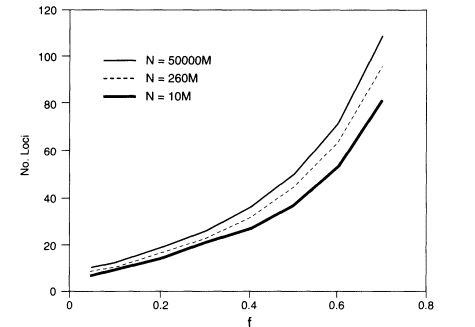
Figure 5.1
The number of loci required to assure with a probability of at
least about 0.99 that no two persons in a randomly mating population share
a profile. Then N is the population number and f is the geometric
mean homozygosity. M = 1,000,000.
average homozygosity in the white population of about 0.20 (Budowle, Baechtel, et al. 1995). About 20 such loci would be required to meet the criterion used for illustrative purposes in the above discussion.
In some cases, the population of interest might be limited to a particular geographic area. For an area with a population of one million, six loci with geometric-mean homozygosities of 0.05 would yield an approximate upper bound of 0.008.
We have discussed two different approaches to the question of uniqueness. Our first approach was to ask for the probability that a given profile is unique. The second and more complicated one asks for the probability that no two profiles are identical. The first question is likely to be asked much more often in a forensic setting.
The number of loci and the degree of heterozygosity per locus that are needed to meet the criteria illustrated above do not seem beyond the reach of forensic science, so unique typing (except for identical twins) may not be far off. How relatives affect determinations of uniqueness will require further analysis, and how the courts will react remains to be seen (see Chapter 6).
Page 139
Statistical Aspects of VNTR Analysis
VNTR alleles differ from one another by discrete steps, but because of measurement uncertainty and the fact that the repeat units are not always the same size, the data are essentially continuous. Therefore, the most accurate statistical model for the interpretation of VNTR analysis would be based on a continuous distribution. Consequently, methods using a continuous distribution and likelihood-ratio theory have been advocated (Berry 1991a; Buckleton et al. 1991; Berry et al. 1992; Evett et al. 1992; Devlin, Risch, and Roeder 1992; Roeder 1994; Roeder et al. 1995). If models for measurement uncertainty become available that are appropriate for the wide range of laboratories performing DNA analyses and if those analyses are suitably robust with respect to departures from the models, we would then recommend such methods. Indeed, barring the development of analytical procedures that render statistical analyses unnecessary, we expect that any problems in the construction of such models will be overcome, and we encourage research on those models.
An analysis based on a continuous distribution would proceed under the hypotheses that the DNA from the evidence sample and from the suspect came from the same person and that they came from different persons. One would seek the relative likelihoods that, with a suitable measure of distance, the bands would be as similar to one another as was observed. At present, however, most presentations of DNA evidence use some form of grouping of alleles. Grouping reduces statistical power but facilitates computation and exposition. A likelihood analysis based on grouping uses an appropriate distance-criterion to calculate the probability that the bands match. That criterion is discussed below.
Determining a Match
According to standard procedure, a match is declared in two stages. Usually the bands in the two lanes to be compared will be in very similar positions or in clearly different positions. If they appear to the analyst to be in similar positions, a visual match is declared. This declaration must then be confirmed by measurement; otherwise, the result of the test is declared to be either an exclusion (no match) or inconclusive. A poor-quality autorad, for example, might result in an inconclusive test. The visual match is a preliminary screen to eliminate obvious mismatches from further study. It excludes some autorads that might pass the measurement criterion as matches if the analyst took into account the correlation of measurement errors (in particular, band-shifting, in which the bands in one lane are shifted relative to those in another), but ordinarily it does not otherwise substitute the analyst's judgment for objective criteria. It would be desirable to develop a way to incorporate any correlation of measurement uncertainty in the objective criterion.
The measurement-confirmation step in the above procedure is based on the
Page 140
size of the band as determined by the molecular-weight standards on the same autorad. The recorded size of this band is, however, subject to measurement uncertainty. Studies at the FBI and the National Institute of Standards and Technology (NIST) have shown that the measurement uncertainty is roughly proportional to the molecular weight (band size is usually measured in units of number of nucleotide pairs rather than in daltons). For example, in the systems published by the FBI and widely used in FBI and other laboratories, the standard deviation of repeated measurements of DNA from the same person is about 1% (Budowle, Giusti, et al. 1991; Mudd et al. 1994). An amount determined by the precision of the measurement is added to and subtracted from the band size, and that determines an "uncertainty window", X ± aX, where X is the measurement of the band size and a is the uncertainty value. The uncertainty window is usually taken to be ± 2.5% of the molecular weight (about 2.5 standard deviations), so that a = 0.025 in this case. This procedure is followed for both the DNA from the evidence sample and that from the suspect. If these two uncertainty windows do not overlap, there is either no match or the result is inconclusive (Figure 5.2a). If the windows overlap, a match is declared (Figure 5.2b). FBI studies (Budowle, Baechtel, et al. 1990; Budowle, Giusti, et al. 1991) report that in 200 within-individual test-band comparisons involving 111 persons, no bands failed to match by this criterion, although Weir and Gaut (1993) report that a slightly larger uncertainty window ( ± 2.8%) was required to obtain the same result for a sample from another laboratory.
The NIST studies (Mudd et al. 1994) provide support for the values found by the FBI. Using measurements obtained by many laboratories over several years, Mudd et al. derived an approximate formula for the standard deviation, s, of a measurement in base pairs (bp):
![]() (5.6)
(5.6)
Expressed as percentages, the values of s are between 0.79 and 0.92 for VNTRs between 2,000 and 6,000 bp.6
The probability of a match between two replicate determinations from the same person increases rapidly with the value of a and is very close to 1 for a = 0.025 (Budowle, Baechtel, et al. 1990; Budowle, Giusti, et al. 1991; Evett, Scranage, and Pinchin 1993) The match window should not be set so small that true matches are missed. At the same time, the window should not be so wide that bands that are clearly different will be declared to match. The 2.5% value used by the FBI, although selected to prevent erroneous nonmatches, nonetheless
6 In the NIST study, 22 labs were sent duplicate pieces of cloth with blood stains on them. The equation is the least-squares fit for the standard deviation of the values obtained by different laboratories. Differences among analysts within a laboratory and differences between laboratories contributed about equally to the total variance. Notice that if the number of base pairs exceeds 6,732, the standard deviation is greater than 1%.
Page 141
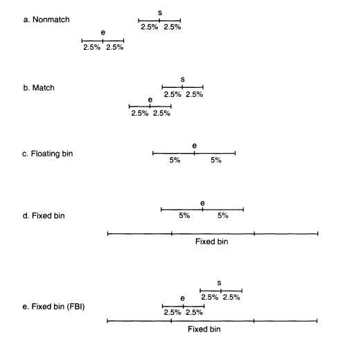
Figure 5.2
An illustration of the matching procedure and the
bin assignment with floating and fixed bins.
seems to deal reasonably well with erroneous matches, too. Bands from the same person are usually very close, within about 1%; those from nonmatching persons are usually far apart. The possibility of coincidental matches for all bands in a multilocus analysis is extremely remote, as the very small match probabilities associated with such a profile indicate (see Chapter 4 for details). The size of the match window should be defined in the laboratory protocol, and not vary from case to case. We believe that technological improvements in laboratory methods should permit the cautious reduction of the match window, as the size of the standard deviation of the measurement declines.
Page 142
The 1992 NRC report recommended that all determinations of matches and bin-allocations be done by objective measurements, following the rules described above (with variations for different laboratories with different systems). The report explicitly stated that visual matches should not be permitted. That is too restrictive, as long as the visual inspection is employed only as a screen. But the use of visual inspection other than as a screen before objective measurement would potentially undermine the basis of the quantitative estimation of the likelihood of a match and should usually be avoided.
An experienced forensic scientist can often use visual screening to recognize band-shifting and other phenomena. For example, degraded DNA sometimes migrates farther on a gel than better-quality DNA (Budowle, Baechtel, and Adams 1991), and an experienced analyst can notice whether two bands from a heterozygote are shifted in the same or in the opposite direction from the bands in another lane containing the DNA being compared. If the bands in the two lanes shift a small distance in the same direction, that might indicate a match with band-shifting. If they shift in opposite directions, that is probably not a match, but a simple match rule or simple computer program might declare it as a match. However, a sophisticated computer program might eventually replace visual matching. As was stated in Chapter 3, if for any reason the analyst by visual inspection overrides the conclusion from the measurements, that should be clearly stated and reasons given.
Binning
Once a match has been declared and confirmed by measurement, it is necessary to estimate the probability of a match on the assumption that the suspect sample and the evidence sample are not from the same source in order to calculate the match probability or likelihood ratio.
Floating bins
One accurate, unambiguous method is to use floating bins (Balazs et al. 1989). Let e and s be the measurements of the DNA bands from the evidence sample and from the suspect. Figures 5.2a and b show that for a match to be declared, the upper end of each uncertainty window must be above the lower end of the other. Therefore, all bands from the DNA of the suspect that satisfy the inequalities (I + a)e > (1 - a)s and (1 + a)s > (1 - a)e would be declared a match. Thus, all such bands within the interval (called the match window)
![]() (5.7a)
(5.7a)
(Weir and Gaut 1993) would have been declared a match, so the analysis must
Page 143
use the frequency (or proportion) of all such bands in the pertinent database. For a << 1, Equation 5.7a is very close to
![]() (5.7b)
(5.7b)
For a = 0.025, Equation 5.7b is sufficiently accurate.
Equation 5.7b determines the approximate floating bin e ± 2 ae, or e ± 0.05e when a = 0.025 (Figure 5.2c). The frequency of that bin is the total proportion of alleles in the database that are within the limits given by Equation 5.7b. With that approach, the floating bin is always the same as the match window. Using a floating bin different from the match window is incorrect; a smaller bin (such as ± 2.5% instead of ± 5% ) will underestimate the match probability; a larger bin will overestimate it.
Fixed bins
Most forensic laboratories have adopted fixed bins, perhaps because of the presumed difficulties of employing floating bins on a wide scale, particularly the necessity of searching the whole database for each calculation (Budowle, Giusti et al. 1991). With current computer-search speeds, these difficulties should be negligible, and the use of floating-bin procedures is statistically preferable because they directly and unambiguously address the central question of estimating the probability of a match. The FBI data set of individual profiles is available on a floppy disk, so laboratories can easily use the FBI database with floating bins.
In the fixed-bin procedures currently employed by many forensic laboratories, alleles of similar size are placed into fixed bins determined by comparing the positions of the evidence bands with bands in a control lane (Figure 5.2d). For example, the alleles at locus D2S44 are grouped into 31 bins for a given database, then adjacent bins with frequencies of fewer than five persons are combined (''rebinned") to produce a grouped frequency distribution for that locus (see Table 4.4) With fixed bins, some statistical power is lost, but there are computational and expository gains.
If the match window is entirely within a bin, the frequency used is that of the bin. When the match window overlaps two or more bins, some method of estimating the frequency is required.
One must distinguish between two uses of fixed bins. Some experts might use them to derive an upper bound to the floating-bin match probability, whereas others might use them to approximate that probability. Distinguishing these two uses is essential whenever the match window around the evidence-sample band, e, specified by Equation 5.7b and usually about 10% wide, overlaps two or more fixed bins. Although bin widths also average about 10%, they vary considerably and some are considerably smaller. To calculate an upper bound, an analyst must add the frequencies of all fixed bins overlapped by the match window, as recommended by the 1992 NRC report. Thus, fixed bins, when used with the
Page 144
criteria described in NRC (1992), yield a more conservative estimate than floating bins. To approximate the floating-bin match probability, we recommend using the fixed bin with the largest frequency among those overlapped by the match window. That approach is based on the observations that both floating and fixed bins are about 10% wide and that bands generally do not cluster around fixed-bin boundaries (Budowle, Giusti et al. 1991; Chakraborty, Jin et al. 1993; Monson and Budowle 1993). The reasons for recommending the procedure are explained below (see also Figure 5.2d).
The FBI and many police agencies follow an approximating procedure that is, on the average, less conservative than the one we recommend (Budowle, Giusti et al. 1991). They use the fixed bin with the largest frequency among those overlapped by the union of the ± 2.5% (5% wide) evidence-sample and suspect-sample windows (Figure 5.2e). However, those windows are each only about one half the width of the match window, so their union could be of any size ranging from about half that of the match window to about equal to that of the match window, depending on the relative positions of e and s. In the extreme case where the evidence-sample and suspect-sample windows barely overlap, three-fourths of this union is included in the match window; otherwise the fraction included is greater. Thus, for every match, at least about three-fourths, but usually most or all of this union is included in the match window. One, two, or more bins might be overlapped.
Monson and Budowle (1993) showed that using the fixed bin with the largest frequency among those overlapped by the ± 2.5% evidence-sample window adequately approximates and is usually more conservative than the match probability calculated from the ± 5% floating bin. Either of the fixed-bin procedures described in the last two paragraphs is more conservative than that of Monson and Budowle (1993), because a larger interval (the ± 5% match window in the first method and the union of the ± 2.5% evidence-sample and suspect-sample windows in the second) might overlap a bin with a higher frequency than does the ± 2.5% evidence-sample window.
We conclude that both the procedure we recommend and that employed by the FBI provide adequate and usually conservative approximations to the correct floating-bin frequency. As Equations 5.7 demonstrate, the match probability depends on e; thus, for this computation the suspect window is irrelevant. The procedure we have recommended is therefore more logical and, on the average, more conservative than that used by the FBI. It is more conservative because a window that is 10% wide might overlap more bins than one that is 5% to 10% wide. Although adding the frequencies of the fixed bins overlapped by the match window is the only procedure that is always conservative, in our view it is excessively cautious (Monson and Budowle 1993) and will usually produce less accurate estimates than our recommendation to take the largest of the overlapped bins. Adding bins would approximately double the best fixed-bin estimate of the match probability for each allele where the match window overlaps two bins.
Page 145
| Box 5.1. Calculating Uncertainty Windows: A Numerical Example Table 4.4 shows the bin sizes for two VNTR loci, D2S44 and D17S79. For locus D17S79, suppose that the evidence-sample band size, e, is measured as 1,200 base pairs (bp). 2.5% of that is 30 bp. The lower limit of the uncertainty window is 1,200-(0.025)(1,200) = 1,170 bp. The upper limit is 1,200 + (0.025)(1,200) = 1,230 bp. The suspect-sample band size, s, is 1,625 bp. The same calculation as above gives a range of 1,584 to 1,666 bp for the uncertainty-window of the sample from the suspect. Since the lower limit of the window for that sample, 1,584 bp, is greater than the upper limit of the window for the evidence sample, 1,230 bp, the bands do not match. Of course, in this case a nonmatch would have been declared visually, and the calculations would be unnecessary. For locus D2S44, suppose that the size of the evidence-sample band is 2,747 bp; the lower and upper ends of the ± 2.5% uncertainty window are then 2,678 and 2,816 bp. Suppose further that the corresponding values for the suspect sample are 2,832, 2,761, and 2,903 bp. Those windows overlap, so a match would be declared. The ± 2.5% evidence-sample window overlaps bins 15 and 16. The approximate match window (from Equation 5.7b), with width 10%, is from 2,610 to 2,884 bp and overlaps bins 15 (freq. = 0.041), 16 (0.040), and 17 (0.086). The bin with the largest frequency among those overlapped by the match window is 17, so our suggested approximate frequency is 0.086. The FBI would use the bin with the largest frequency among those overlapped by the union of the evidence-sample and suspect-sample uncertainty windows, 2,678 to 2,903 bp; the union overlaps bins 15, 16, and 17. Again the bin with the highest frequency is 17. An upper bound to the fixed-bin match probability is the total frequency of the three bins overlapped by the match window; that frequency is 0.167. The floating-bin frequency is the proportion of bands in the database that lie in the match window, and is about 0.071. The fixed-bin estimate, 0.086, is therefore slightly conservative. (Note: the floating-bin frequency cannot be calculated from Table 4.4, but requires the FBI database.) If the more accurate Equation 5.7a had been used, the match window would have been 2,613 to 2,888 bp. The widely used approximation, Equation 5.7b, is clearly quite accurate, although the exact formula would be theoretically preferable. |
Page 146
Confidence Intervals for Match Probabilities
Match probabilities are calculated from a database. Those data are a sample from a larger population, and another sample might yield different match probabilities. To account for the fact that match probabilities are based on different databases and might change if another data set were used, it is helpful to give confidence intervals for those probabilities. A confidence interval is expected to include the true value a specified percentage of the time. In symbols, a 100(1 - a)% confidence interval is expected to include the true value 100(1 - a )% of the time. Typical values are 95% (a = 0.05) or 99% (a = 0.01). The confidence interval will depend on the genetic model, the actual probabilities, and the size of the database. We consider only the simplest case, a population in HW and LE proportions.
For such a population, the probability of a multilocus genotype is the product of the constituent allele frequencies, which are estimated from the database, with a factor of 2 included for each heterozygous locus involved (see Chapter 4). The product form of the relation suggests that it is most convenient to find a confidence interval for the natural logarithm of the probability and then transform it back to the probability, as is often done in data analysis (see Sokal and Rohlf 1981).
The contribution to the match probability of a single homozygous locus is pi2 (or 2pi if a conservative estimate is desired) and, for a heterozygous locus, it is 2pipj. In practice, the true probability is unknown and is replaced by the estimate, ![]() , which is taken to be the proportion of the k-th allele in the database of N persons (2N genes per locus). We approximate the expectation of each logarithm by the logarithm of the expectation. The approximate variances of the logarithms are
, which is taken to be the proportion of the k-th allele in the database of N persons (2N genes per locus). We approximate the expectation of each logarithm by the logarithm of the expectation. The approximate variances of the logarithms are
![]() (5.8a)
(5.8a)
![]() (5.8b)
(5.8b)
![]() (5.8c)
(5.8c)
If Npi >> I for each allele and every locus, the logarithm of the genotype frequency is approximately normally distributed (Cox and Snell 1989). Because of the independence of the loci, the variance of the logarithm of the multilocus estimate is the sum of the values for each locus. If za is the standard-normal deviate associated with a symmetric confidence interval of 100(1- a )%, then the confidence interval for the logarithm of the genotypic frequency is equal to the estimated value ± zas, where s is the square root of the multilocus variance. These limits are then transformed back by antilogs.
A similar procedure was given by Chakraborty, Srinivasan, and Daiger (1993).
If more loci are added, the estimated probability will be smaller, but additional variability in the estimate implies that on the log scale the interval will be wider.
Page 147
A smaller database also will lead to wider intervals. The width of the confidence interval on the log scale is inversely proportional to the square root of the size of the database. Thus, for a database one fourth as large as the one in Box 5.2, the confidence limits would be - 17.263 ± (1.96)(0.329)(2). On the original scale, the limits are 8.76 x 10⁻⁹ and 1.156 x 10⁻⁷, a range of about 13-fold, which is more than three times as large as the confidence interval for the database in Box 5.2. We can also write confidence intervals for values calculated with Equations 4.10.7
| Box 5.2. Calculating Confidence Limits: A Numerical Example As a numerical example, consider again the data for the white population illustrated in Box 4.3, using data from Table 4.8. The profile is A6 - B8B14 C10C13 D9D16. The A-locus variance component is estimated to be
For the B-locus, the component is
For the C-locus, the component is 0.01475, and for D it is 0.03807. Adding those four components yields a sum of 0.10820, the square root of which is 0.32893. The estimated genotype frequency (Box 4.3) is 3.182 x 10⁻⁸; its natural logarithm, (2.303 log10), is -17.263. For a 95% confidence interval, za = ± 1.96, so the confidence limits of the logarithm are - 17.263 ¹ (1.96)(0.329). Taking antilogs (exponentiating), the confidence limits for the match probability are 6.06 x 10⁻⁸ and 1.67 x 10⁻⁸. The width of the 95% confidence interval is about a factor of 3.6, or roughly a factor of 1.9 in either direction. |
7 If Equations 4.4 or 4.10 are used to evaluate match probabilities, a prescription for calculating confidence intervals can be similarly derived, although the detailed formulae will be somewhat different. Since knowledge of the range of reasonable values of ![]() is obtained from an accumulating body of population-genetics studies, one might give a range of confidence intervals based on a range of values of
is obtained from an accumulating body of population-genetics studies, one might give a range of confidence intervals based on a range of values of ![]() . Alternatively, when applying Equations 4.10. one could obtain a conservative approximation to match probabilities by using a value of
. Alternatively, when applying Equations 4.10. one could obtain a conservative approximation to match probabilities by using a value of ![]() that is slightly larger than that found in most studies. For example, for a confidence interval based on Equations 4.10. at each locus the contribution to the variance of the estimated value of the logarithm of Equation 4.10a equals approximately
that is slightly larger than that found in most studies. For example, for a confidence interval based on Equations 4.10. at each locus the contribution to the variance of the estimated value of the logarithm of Equation 4.10a equals approximately
![]()
for Equation 4.10b, the corresponding formula is
![]()
Page 148
Although calculation of confidence intervals is desirable, they do not include the effects of all the sources of error. A more inclusive estimate of uncertainty, which is usually larger, is considered later in the chapter.
Alleles with Low Frequency
VNTRs have a very large number of alleles. Consequently, some bins—especially those at the ends of the size distribution for a locus—have very low frequencies. An estimate of an allele frequency can be very inaccurate if the allele is so rare that it is represented only once or a few times in a database; and some rare alleles might not be represented at all. Several procedures have been suggested to alleviate the problems caused by such inaccuracies. One approach is to add 0.5 to the observed number of occurrences of each rare allele (Cox and Snell 1989); another is to replace all rare-allele proportions by an arbitrary upper bound, as has been done for paternity analysis (Walker 1983, p 449). That was also recommended by Chakraborty (1992) and for STRs, by Evett et al. (1996).
It is common in some statistical tests to pool very rare classes, and that is what the FBI has done by rebinning. If a bin in the database contains fewer than five entries, it is pooled with adjacent bins so that no bin has fewer than five. We recommend this procedure for VNTRs and for other systems in which an allele is represented fewer than five times in the database. For a floating-bin analysis, the bin frequency is determined only after the evidence sample is typed. A similar expedient for rare alleles is to use the maximum of 5 and k, where k is the actual number of alleles from the database that fall within the match window.
Rare alleles can produce substantial departures from HW proportions, even if the populations from which they are drawn are in random-mating proportions. This is illustrated in the data in Table 4.4. Estimates of ![]() ii obtained by randomly combining the data from Table 4.4 are all positive, as expected, and are each less than 0.004. Estimates of
ii obtained by randomly combining the data from Table 4.4 are all positive, as expected, and are each less than 0.004. Estimates of ![]() ij are more variable and can be either positive or negative; about 1/5 of the values are outside the range - 0.1 to 0.1. Large negative values can mean that HW calculations can be serious underestimates and thus biased against the defendant. However, these values are the result of random fluctuations between databases. In actual populations, we expect
ij are more variable and can be either positive or negative; about 1/5 of the values are outside the range - 0.1 to 0.1. Large negative values can mean that HW calculations can be serious underestimates and thus biased against the defendant. However, these values are the result of random fluctuations between databases. In actual populations, we expect ![]() ij to be positive unless it is very close to zero.
ij to be positive unless it is very close to zero.
Individual Variability and Empirical Comparisons
Confidence intervals derived from the simplifying assumptions of sampling theory do not take account of all possible sources of uncertainty that can affect the accuracy of a match probability or likelihood ratio. To examine the degree to which other sources of variation may affect the accuracy of our calculations, we have looked to empirical studies.
The FBI has compiled many data from the United States and other parts of
Page 149
the world (FBI 1993b; Budowle, Monson, Giusti, and Brown 1994a, 1994b). We can use those data to examine frequencies of a given genotype in different data sets.
We are mainly concerned with the effects of population subdivision, leading to different allele frequencies in different areas or in people with different ethnic backgrounds. Such differences are obscured in the averages. We examine only allele frequencies, because multilocus genotypes are much too rare to study. But the close agreement of the data with HW and LE proportions (Chapter 4), together with conservative assumptions, lend credence to our analyses.
Geographical Subdivision
One question is whether local regions differ appreciably from the national average. The FBI has compiled data from different sources throughout the world. One representative example is a comparison between blacks in the United States as a whole and those in Georgia. Assume that the source of evidence DNA from a particular crime in Georgia is known to be black. To make the most appropriate estimate of the probability that a profile from a randomly selected black person from this area would match the evidence profile, we would use the Georgia database. But suppose that we do not have local data and use the national average instead. How much of an error would that entail?
The relevant data (from FBI 1993b) are graphed in Figure 5.3. Each point on the graph represents a specific genotype for one or more of four VNTR loci, D1S7, D2S44, D4S139, and D10S28. For each genotype on the graph, the estimated frequency from the general US black database is given by the ordinate; its estimated frequency in the local Georgia database is given by the abscissa. In calculating the genotypic frequencies, LE and HW proportions were assumed, and single bands were assigned a frequency of 2p.8 The two lines on either side of the diagonal represent 10-fold deviations from the expected proportions. The US population is probably more heterogeneous than the Georgia subset. The graph shows that if one were investigating a crime in Georgia but used nationwide figures, the estimate would practically always lie between the two lines, that is, it is within a factor of 10 either way from the frequency of the same profile in the more relevant local database.
As stated earlier, the points on these graphs are calculated from the databases under the assumptions that HW and LE ratios prevail within the population
8 Figures 5.2-5.4 appear to show more very large values than expected (near the lower left corner). That is caused by the conventions used in the preparation of the graphs. First, each single band was given a value of twice the bin frequency (that is, the 2p rule was applied). Second, some of the points are for small numbers of loci, sometimes as few as one. Third, greater errors are likely to occur in measuring very large and very small fragments; therefore, such fragments were each assigned a value of one. In general, the more loci represented by a data point, the farther to the upper right the point lies.
Page 150
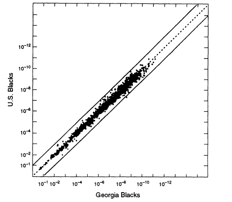
Figure 5.3
A scatter plot for US black populations. Each point represents a specific genotype
from one to four VNTR loci, whose estimated frequency in the overall US black
population is given by the ordinate and in the Georgia black population by the abscissa.
The upper and lower lines represent values that deviate from equality by a factor of 10.
Note: 10-6 = 1/106 = 0.000001. From FBI (1993b, p 1233).
represented in each database. Departures from these assumptions could, of course, lead to greater uncertainty. In Chapter 4, however, we noted that typical values of ![]() are less than 0.01 and departures from LE are similarly small. Therefore, we believe that the uncertainties caused by deviations from HW and LE expectations are much less than those caused by differences in allele frequencies in different subgroups.
are less than 0.01 and departures from LE are similarly small. Therefore, we believe that the uncertainties caused by deviations from HW and LE expectations are much less than those caused by differences in allele frequencies in different subgroups.
The FBI compendia (FBI 1993b; Budowle, Monson, Giusti, and Brown 1994a, 1994b) contain a large number of graphs with many different comparisons. Figure 5.3 is typical of several other geographical comparisons. Geographical data for whites and Hispanics are in general agreement with those for blacks. We conclude that individual within-race profile frequencies from different geographic
Page 151
areas in the United States usually differ by less than a factor of 10 in either direction.
Differences Among Subgroups
The US white population consists of people of various European origins who have been partially mixed in the "melting pot." How much difference does this substructure make? It is difficult to identify relevant homogeneous groups within the United States. A better way to answer the question is to use data from Europe; those data better reflect the characteristics of the ancestral groups and should exaggerate between-group differences that have been diluted in the mixing of populations in the United States. Because of its large database, we compare the data set from Denmark with that from the United States (Figure 5.4). As the graph shows, if we substitute average frequencies for US whites for frequencies from the Danish data set, the error is almost always less than 10-fold in either direction. Graphs of Swiss, German, Norwegian, Spanish, and French data show similar patterns when compared with the United States. The percentage deviations tend to be larger in the upper right-hand part of the graphs—that is, where the probabilities become small. With probabilities of one in 100 million or less, an error of 10-fold either way is not likely to affect the conclusion.
The European populations have mixed less than the corresponding US groups that descended from European migrants. Therefore, the effects of subdivision should be less among white populations in the United States than in Europe. It seems safe to say that for those groups, an estimate using a nationwide rather than a subgroup database is likely to be less than 10-fold too low or too high. Data for Hispanics and East Asians are similar.
Different Races
When we compare data from different racial groups, a different picture emerges from that found within racial groups—the profile frequencies can differ considerably. Figure 5.5 compares US whites and blacks. Although the great majority of the points lie within a ± 10-fold range, an appreciable fraction are found outside this range. If, for example, we used the white database when we should have used the black, the error would sometimes be greater than 10-fold (that is, a substantial fraction of the data points are outside the two lines on either side of the diagonal in the figure), and a few points differ by 100-fold or more. That suggests a conservative procedure that can be used if it is not known whether the perpetrator is black or white: a match probability could be calculated from both databases and the higher of the two values used. If only one database is used, it might be the wrong one, and the result might be misleading.
It is not surprising that differences between races are considerably larger than those between subgroups within races (Devlin and Risch 1992; Devlin,
Page 152
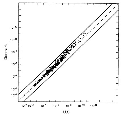
Figure 5.4
A scatter plot for the white population. The abscissa gives estimated frequencies in the US
white population and the ordinate those in a Danish population. White frequencies are from
Cellmark; Danish frequencies from Institute of Forensic Genetics in Copenhagen. From
FBI (1993b, p 1267).
Risch, and Roeder 1993, 1994). That has been known by population geneticists for a long time and for various genes. The 1992 NRC report relied on a single study (Lewontin 1972) that appeared to support the opposite view, but that study has not been confirmed by other, more extensive ones (for example, Latter 1980). The 1992 report took the view of Lewontin and Hartl (1991) that examination of differences in databases from different racial groups might actually underestimate the degree of divergence within races, rather than overestimate it as we have seen to be the case from the VNTR studies discussed above. The recent compilations by the FBI, as well as numerous other studies (e.g., Hartmann et al. 1994), confirm the intuitively reasonable expectation that differences between ethnic groups within races are smaller than differences between races. But the
Page 153
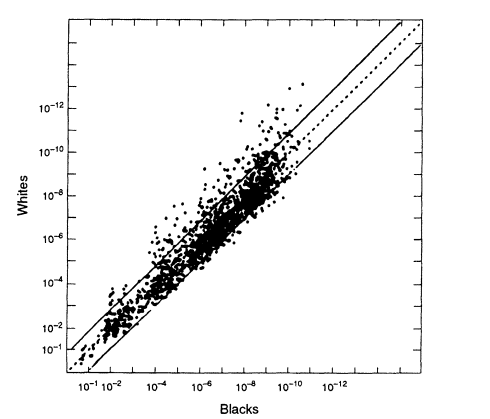
Figure 5.5
A scatter plot comparing the estimated white population
frequencies (ordinate) with the black population (abscissa). Note the
considerably greater spread than in Figures 5.2 and 5.3, which plot data
from within the same racial group. From FBI ( 1993b. p 1230).
far more important conclusion, and the one that makes VNTR and other forensic loci so useful, is that most of the variation is not among groups but among persons, as population geneticists, including Lewontin (1972), have repeatedly emphasized.
We have referred to only some of the available data above. Several other studies have used deliberately wrong or artificially stratified databases and showed that such manipulations do not produce grossly wrong results (Evett and Pinchin 1991; Berry, Evett, and Pinchin 1992).
As mentioned earlier, in the data compiled by TWGDAM there was only one four-locus match in the white population and one in the Hispanic population among 58 million pairwise comparisons. There were no five- or six-locus matches.
Page 154
That was not true for the American Indian population, where two four-locus matches were found among 1.7 million pairs. Those were not instances where the same person was entered twice into the database, because the profiles did not match at the other loci tested. As we have emphasized earlier, there is considerably more subdivision in American Indians, so four-locus matches within a tribe are not as unusual (R. Chakraborty, unpublished data).
The data and studies that we have reviewed support the argument that multilocus VNTR comparisons are very powerful tests of identity. Unless there is reason to believe that close relatives are involved or that the suspect and donor of the evidence DNA, if not the same person, are from the same subpopulation, the product rule (with the 2p rule) is appropriate (see Chapter 4).
The data for PCR-based systems are far more limited than those for VNTRs. However, the numbers are increasing. Chakraborty, Jin, et al. (1995) show graphs of different populations within racial groups for Polymarkers, plotted in the manner of Figures 5.3 to 5.6. The numbers for Polymarkers are much smaller than those for VNTRs, but as with VNTRs, the points all fall within 10-fold above or below the line corresponding to perfect agreement. Comparable data exist for STRs.
As mentioned before, the graphs in Figures 5.3 and 5.4 assume HW and LE. On the average, as we have repeatedly emphasized, departures from these assumptions are small. Yet, with several loci, despite some cancellation, small errors can accumulate. That is most important for rare alleles, where random fluctuations can generate appreciable departures from HW and LE.
In a recent study of the TWGDAM data, Chakraborty (personal communication) has calculated the values of ![]() ij for VNTRs. Even though the mean value is close to zero and the distribution is approximately symmetrical, individual values show appreciable departures, especially for very rare alleles. The variability is mainly, if not entirely, due to uncertainties in the databases, but such variations may also occur in the population if there is localized subdivision.
ij for VNTRs. Even though the mean value is close to zero and the distribution is approximately symmetrical, individual values show appreciable departures, especially for very rare alleles. The variability is mainly, if not entirely, due to uncertainties in the databases, but such variations may also occur in the population if there is localized subdivision.
More Conservative Formulae
Some workers (Balding and Nichols 1994, 1995) have advocated the use of Equations 4.10 rather than the simpler Equations 4.1, which assume HW proportions (see Chapter 4). Figure 5.6 illustrates the effect of using Equations 4.10 for a rather extreme example (Roeder et al. 1995). On the ordinate are the frequencies of various genotypes for an artificial 50:50 pooled mixture of whites and blacks; on the abscissa are frequencies for whites. If we assume that the evidence DNA is from a white person, and if we falsely assume that the pooled mixture of whites and blacks is in HW and LE proportions, then the graph shows the range of error that would exist if the pooled database were used instead of the more appropriate database for whites. In the top graph in the figure, a point that is below and to the right of the diagonal line overestimates the true probability
Page 155
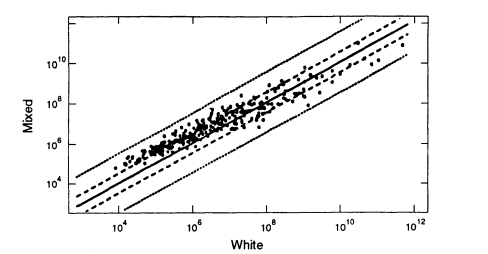
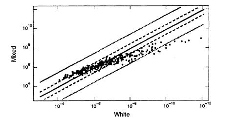
Figure 5.6
A scatter plot comparing the white population (abscissa)with an equal
mixture of whites and blacks (ordinate). In the upper graph, the HW rule
was used; in the lower, Equations 4.10 with ![]() . The dashed
. The dashed
lines represent deviations by a factor of 5 and the dotted lines
by a factor of 15. Data from Lifecodes (Roeder et al. submitted).
of a match (that is, it errs in favor of the defendant). The majority of the points in the regions of higher probabilities are above the 45° line; that is, they are biased against the defendant. That is the effect that was of concern in the 1992 NRC report, but with respect to ethnic differences within racial groups rather
Page 156
than between racial groups. We have chosen an extreme example for illustration. Even so, all the points are within 15-fold of the 45° diagonal line in the graph.
The bottom graph in Figure 5.6 shows the effect of using Equations 4.10 for the mixed population rather than using the HW formula, Equation 4.1. The value of ![]() was taken to be 0.01, which is the value estimated from this data set (Roeder et al. 1995). It is clear from the graph that using Equations 4.10 usually leads to a conservative estimate, except for the higher probabilities shown in the lower left part of the graph. That makes sense, for it is clear from Equations 4.10 that when p is large,
was taken to be 0.01, which is the value estimated from this data set (Roeder et al. 1995). It is clear from the graph that using Equations 4.10 usually leads to a conservative estimate, except for the higher probabilities shown in the lower left part of the graph. That makes sense, for it is clear from Equations 4.10 that when p is large, ![]() has little effect on profile-frequency estimates.
has little effect on profile-frequency estimates.
We conclude that, even if an artificial, intentionally inappropriate database of mixed profiles from whites and blacks is used, Equations 4.10 are conservative. We further note that when fixed bins are used in the manner recommended in the section in this chapter on statistical aspects of VNTR analysis, the procedure is usually conservative, and that applying the 2p rule increases the conservatism of the method. Finally, using Equations 4.10 with fixed bins adds to the conservatism.
To summarize: Within a racial group, geographic origin and ethnic composition have very little effect on the frequencies of forensic DNA profiles, although there are larger differences between major groups (races). It is probably safe to assume that within a race, the uncertainty of a value calculated from adequate databases (at least several hundred persons) by the product rule is within a factor of about 10 above and below the true value. If the calculated profile probability is very small, the uncertainty can be larger, but even a large relative error will not change the conclusion. If there is good reason to think that the suspect and the source of the evidence are from the same subpopulation, Equations 4.10 can be used.
The Ceiling Principles
The 1992 NRC report assumed that population substructure might exist and recommended procedures for calculating profile frequencies that could be expected to be sufficiently conservative to accommodate the presence of substructure. Two such procedures are recommended in the 1992 report, the ''ceiling principle" and the "interim ceiling principle."
The ceiling principle (NRC 1992, p 82-85) places a lower limit on the size of the profile frequency by giving thresholds for the allele-frequency values used in the calculation. To determine the thresholds, the report recommended that 100 persons be sampled from each of 15-20 genetically homogenous populations spanning the racial and ethnic diversity of groups represented in the United States. For each allele the highest value among the groups sampled, or 5%, whichever was larger, would be used. Then the product rule would be applied to those values to determine the profile frequency. The choice and sampling of the 15-20 populations was to be supervised by the NCFDT (see Chapter 3), which has not come into being. The necessary ground work for applying the
Page 157
ceiling principle has not been done, and there have been few attempts to apply it. We share the view of many experts who have criticized it on practical and statistical grounds and who see no scientific justification for its use.
The 1992 report recommended that until the ceiling principle could be put into effect, the interim ceiling principle be applied. In contrast to the ceiling principle, the interim ceiling principle has been widely used and sometimes misused. The rule (NRC 1992, p 14-15, 91-93) is: "In applying the multiplication rule, the 95% upper confidence limit of the frequency of each allele should be calculated for separate US 'racial' groups and the highest of these values or 10% (whichever is the larger) should be used. Data on at least three major 'races' (e.g., whites, blacks, Hispanics, east Asians, and American Indians) should be analyzed." The report also stated that the multiplication (that is, product) rule should be applied only when there is no significant departure from HW and LE, even though the ceiling principle was introduced specifically to accommodate deviations from HW and LE.
If the interim ceiling principle is applied to four loci, the minimum probability, assuming that there are no single bands, is [2(0.1)(0.1)]4 = (1/50)4 = 1/6,250,000. With five loci the minimum probability becomes about one in 300 million. But if the 2p rule is used for single bands and any locus found to depart from HW proportions is not used, the probability can be much larger. For example, if only three loci are used and one is homozygous, the minimum is 2(0.1)(1/50)2 = 1/12,500.
Is the interim ceiling principle logical? Is it unnecessarily conservative? In view of all the accumulated data we have discussed, is it needed? The interim ceiling principle has the advantage that in any particular case it gives the same answer irrespective of the racial group. That is also a disadvantage, because it does not permit the use of well-established differences in frequencies in different races; it is inflexible and cannot be adjusted to the circumstances of a particular case.
The ceiling principles have been widely discussed, usually critically (Chakraborty and Kidd 1991; Cohen 1992; Morton 1992, 1995; Evett, Scranage, and Pinchin 1993; Kaye 1993, 1995a; Lempert 1993; Weir 1993a; Balding and Nichols 1994; Devlin, Risch, and Roeder 1994; Lander and Budowle 1994; TWGDAM 1994c; Morton 1995). Here are some of those criticisms:
· The 10% value is completely arbitrary, and there is no scientific justification of its choice as a ceiling value.
· Although calculation of an upper 95% confidence limit for an individual allele is justified as a standard statistical procedure, multiplication of those values is not.
· The ceiling principles do not make use of the large amount of allele-frequency data now available from different groups and subgroups.
· They do not make use of standard procedures long used by population geneticists to study subdivided populations.
Page 158
· It is excessively conservative. (Actually it is not always conservative, for one can contrive examples in which it is not [Slimowitz and Cohen 1993], but in realistic examples it is conservative.)
· The report's lack of specific instructions as to which population groups should be included has led some experts and attorneys to focus on extreme examples, perhaps involving small databases with large sampling errors or irrelevant populations; that practice was not foreseen by the writers of the 1992 report.
We agree with the criticisms listed above. Our view is that sufficient data have been gathered that neither ceiling principle is needed. We have suggested alternative procedures, all of which are conservative to some degree. We believe that estimates based on the formulae outlined in Chapter 4—and with proper attention to uncertainties—are now appropriate. In special cases in which there is no appropriate database, such as for some American Indian tribes, the estimates (based on the methods in this report) for several related groups should be used.
TWGDAM (1994c) has recently issued a report on the ceiling principle. TWGDAM "cannot recommend the application of the ceiling principle. The basis for the need for a ceiling principle is flawed. . . . The current methods employed by forensic scientists have been demonstrated to be robust scientifically" (p 899).
If the interim ceiling principle is used despite that recommendation, TWGDAM recommends an approach intended to overcome some of the criticisms of the 1992 NRC report. The recommended approach differs from that in the 1992 report in several ways:
· When the measurement error spans a fixed-bin border, take the frequency of the most frequent of the bins instead of summing the overlapped bins, as recommended by the 1992 report.
· Native-American databases are not to be used to generate values for the ceiling; the groups to be used are whites, blacks, Hispanics, and east Asians.
· The multiple of the standard deviation for an upper 95% confidence limit should be 1.64, not 1.96, which was given in a footnote on page 92 of the 1992 report. NRC (1992) confused one-tailed and two-tailed confidence coefficients.
We agree with the TWGDAM recommendations and add the following interpretations, which we believe are consistent with the 1992 report.
· The ceiling principles are intended for criminal, not civil cases. They are therefore inappropriate for paternity testing, unless that is part of a criminal proceeding.
· The ceiling principles were intended for VNTRs with many alleles, no one of which has a very high frequency. They are not applicable to PCR-based systems, which ordinarily have few alleles. For example, applying the upper 95% confidence limit produces allele frequencies that add up to more than one, and,
Page 159
with two alleles, to heterozygote frequencies that can be greater than the HW maximum of 1/2.
· As originally presented (NRC 1992, p 91), the ceiling principle would use only those loci not differing significantly from HW and LE. But populations with the least reliable numbers (that is, the smallest databases) are the very ones most likely not to show a statistically significant departure from HW and LE. Thus, an analyst who uses the interim ceiling principle will often be forced to reject more reliable loci in favor of less reliable ones. Furthermore, the purpose of the ceiling principles is to allow for differences in allele frequencies in different subgroups, for which HW and LE are insensitive measures. Therefore, we believe that all loci in the selected databases should be used in the calculation.
In summary, the procedures we have recommended in Chapter 4 are based on population genetics and empirical data and can encompass suitable degrees of conservatism. With such procedures available, we believe that the interim ceiling principle is not needed and can be abandoned.
Direct Count from a Database
The 1992 NRC report stated (p 91) that "the testing laboratory should check to see that the observed multilocus genotype matches any sample in the population database. Assuming that it does not, it should report that the DNA pattern was compared to a database of N individuals from the population and no match was observed, indicating its rarity in the population." The Committee noted that if there were no occurrences of a profile in 100 samples, the upper confidence limit is 3%. It went on to say (p 76) that "such estimates produced by straightforward counting have the virtue that they do not depend on theoretical assumptions, but simply on the sample's having been randomly drawn from the appropriate population. However, such estimates do not take advantage of the full potential of the genetic approach."
The ceiling method uses random-mating theory but does not make full use of population data. The counting method does not even combine allele frequencies and thereby loses even more information. In addition, very small probabilities cannot be estimated accurately from samples of realistic size; modeling is required. In fact, most profiles are not found in any database, so there must be a convention as to how to handle zeros. Since we believe that the abundant data make the ceiling principles unnecessary, this is true a fortiori for the direct counting method.
Some statisticians and others have questioned the accuracy of using population-genetics theory that incorporates estimated allele distributions in forensic calculations. Somewhat comparable calculations are available that do not use this information. For a Poisson distribution, an upper 100(1 - a)% confidence limit L for the expected number of events when zero events have been observed
Page 160
is L = - ln(a). For a 95% confidence limit, a = 0.05 and L = 3. For illustration, the TWGDAM data included about 7,000 persons in the white database. That yields (7,000)(6,999)/2 = 24.5 million pairs of profiles. Only one four-locus match was found and none for five or more. Let us assume that all persons were tested at five loci—the same five loci—and regard these pairs as a random sample. Then a Poisson approximation similar to that leading to Equation 5.5 (but without assuming HW and LE) leads to the conclusion that an upper 95% confidence limit for the probability of a match between suspect and evidence DNA at those five loci is 3/(24.5 million), or about 1 in 8 million. This calculation illustrates the possibility of procedures that do not employ estimated allele distributions and population-genetics theory but still give very small match probabilities, provided that sufficiently large databases of genotype profiles are available.
However, such a method is inappropriate, and we do not recommend it. It gives an approximate upper bound to the mean value, but not conditioned on the particular profile in question; it does not answer the question we are most interested in, the probability of a match of the particular evidence and suspect profile. It has not been demonstrated to be robust with respect to various database problems; for example, the same loci may not always have been tested. Also, it does not use available information about allele frequencies and thus does not permit sharper inferences conditional upon that information. Finally, the value is strongly dependent on the size of the database.
The population-genetic assumptions that we use are robust, are accurate within the limits discussed elsewhere in this report, and make sensible use of information about allele frequencies.
Conclusions and Recommendations
Statistical Issues
Confidence limits for profile probabilities, based on allele frequencies and the size of the database, can be calculated by methods explained in this report. We recognize, however, that confidence limits address only part of the uncertainty. For a more realistic estimate, we examined empirical data from the comparison of different subpopulations and of subpopulations with the whole. The empirical studies show that the differences between the frequencies of the individual profiles estimated by the product rule from different adequate subpopulation databases (at least several hundred persons) are within a factor of about 10 of each other, and that provides a guide to the uncertainty of the determination for a single profile. For very small estimated profile frequencies, the uncertainty can be greater, both because of the greater relative uncertainty of individually small probabilities and because more loci are likely to be multiplied. But with very small probabilities, a large relative error is not likely to change the conclusion.
Page 161
Database Searches
If the suspect is identified through a DNA database search, the interpretation of the match probability and likelihood ratio given in Chapter 4 should be modified.
Recommendation 5.1: When the suspect is found by a search of DNA databases, the random-match probability should be multiplied by N, the number of persons in the database.
If one wishes to describe the impact of the DNA evidence under the hypothesis that the source of the evidence sample is someone in the database, then the likelihood ratio should be divided by N. As database searches become more extensive, another problem may arise. If the database searched includes a large proportion of the population, the analysis must take this into account. In the extreme case a search of the whole population should, of course, provide a definitive answer.
Uniqueness
With an increasing number of loci available for forensic analysis, we are approaching the time when each person's profile will be unique (except for identical twins and possibly other close relatives). Suppose that, in a population of N unrelated persons, a given DNA profile has probability P. The probability (before a suspect has been profiled) that the particular profile observed in the evidence sample is not unique is at most NP.
A lower bound on the probability that every person is unique depends on the population size, the number of loci, and the heterozygosity of the individual loci. Neglecting population structure and close relatives, 10 loci with a geometric mean heterozygosity of 95% give a probability greater than about 0.999 that no two unrelated persons in the world have the same profile. Once it is decided what level of probability constitutes uniqueness, appropriate calculations can readily be made.
In any particular case, the chance that the DNA profile for the evidence sample is unique is of more concern than the chance that all DNA profiles are unique. Hence, the calculation in the first paragraph will be the one more often employed.
Matching and Binning
VNTR data are essentially continuous, and, in principle, a continuous model should be used to analyze them. The methods generally used, however, involve taking measurement uncertainty into account by determining a match window. Two procedures for determining match probabilities are the floating-bin and fixed-bin methods. The floating-bin method is statistically preferable but requires
Page 162
access to a computerized database. The fixed-bin method is more widely used and understood, and the necessary data tables are widely and readily available. When our fixed-bin recommendation is followed, the two methods lead to very similar results. Both methods are acceptable.
Recommendation 5.2. If floating bins are used to calculate the random-match probabilities, each bin should coincide with the corresponding match window. If fixed bins are employed, then the fixed bin that has the largest frequency among those overlapped by the match window should be used.
Ceiling Principles
The abundance of data in different ethnic groups within the major races and the genetically and statistically sound methods recommended in this report imply that both the ceiling principle and the interim ceiling principle are unnecessary.
Further Research
The rapid rate of discovery of new markers in connection with human gene-mapping should lead to many new markers that are highly polymorphic, mutable, and selectively neutral, but which, unlike VNTRs, can be amplified by PCR and for which individual alleles can usually be distinguished unambiguously with none of the statistical problems associated with matching and binning. Furthermore, radioactive probes need not be used with many other markers, so identification can be prompt and problems associated with using radioactive materials can be avoided. It should soon be possible to have systems so powerful that no statistical and population analyses will be needed, and (except possibly for close relatives) each person in a population can be uniquely identified.
Recommendation 5.3. Research into the identification and validation of more and better marker systems for forensic analysis should continue with a view to making each profile unique.
Appendix 5A
Mixed stains introduce a number of complexities. We limit our consideration to cases in which the stain comes from two persons, but only one suspect is identified. The case where four bands are observed, two of which match the suspect, was given in the text. Here we consider circumstances in which fewer than four bands are found in the evidentiary DNA. This may mean that either the suspect or the other contributor to the stain produced a single band. Thus, the 2p rule may be needed. It is also possible that there are only two bands, but other loci indicate that the stain is mixed. These cases are summarized in Table 5.1.
Page 163
| TABLE 5.1 Likelihood Ratios for Mixed Stainsa | |||
| Crime scene | Suspect | Rule | Likelihood Ratio |
| A1A2A3A4 | A1A2 | — |
|
| A1A2A3 | A2A3 | 2p |
|
| p2 |
| ||
| A1A2A3 | A1 | 2p |
|
| p2 |
| ||
| A1A2 | A1A2 | 2p |
|
| p2 |
| ||
| A1A2 | A1 | 2p |
|
| p2 |
| ||
| aFor each combination of crime-scene and suspect genotypes, the likelihood ratio is given for each of two rules for dealing with single bands (or homozygotes). | |||
Appendix 5B
If the database is not homogeneous, that is, if P(Mi) is different for different values of i, then the inequality in Equation 5.3 is still valid, so
![]() (5.9)
(5.9)
where P(Mi) can be evaluated by the methods of Chapter 4. Many of the terms in the sum will be the same. In the simplest case, in which the database contains N persons, all with the same ethnic background, the effect is just to multiply an individual match probability by N, leading to Equation 5.3.
If we assume that the database consists of n1 whites and n2 blacks, then Equation 5.9 simplifies to
![]() (5.10)
(5.10)
where W denotes the event that a randomly selected white profile matches the evidence-sample profile and B denotes the same match event for a randomly selected black profile.
Page 164
Remark. An approximation that will often be somewhat closer to P(M) than Equation 5.9 is
![]() (5.11)
(5.11)
That approximation will give approximately the same answer as Equation 5.9 when SiP(Mi) is small, and that is the case of practical importance.
The event M involves all markers tested, both those employed for identification purposes and any additional markers used for confirmation. If we let Mi,1 denote the event of a match of the i-th profile on the initial batch of markers tested for the purpose of the database search, and Mi,2 the event of a match of the i-th profile on the subsequent markers tested, then under the assumption of linkage equilibrium, P(Mi) = P(Mi,1P)P(Mi,2). That same factorization would hold under the assumption of linkage equilibrium for an arbitrary division of the markers into two subsets.
From a Bayesian viewpoint, there are other methods to deal with database searches, although the final result is much the same as that given above (see also Balding and Donnelly 1995). Although the assignment of prior probabilities is problematic and appears to have been used rarely if at all in criminal forensic investigations in the United States, some related ideas can be useful in clarifying certain issues. Let Q be the probability of the event E that some person whose profile is in the database left the evidence sample, with 1 - Q being the probability of event Ec that the evidence sample was left by someone whose profile is not in the database. Suppose that there is a match between the evidence-sample profile and at least one profile in the database. Assuming that ![]() and
and ![]() , where P(M) is evaluated as above, we find the posterior odds that the evidence sample was left by someone whose profile is in the database to be
, where P(M) is evaluated as above, we find the posterior odds that the evidence sample was left by someone whose profile is in the database to be ![]() . Since the posterior odds equals the prior odds times the likelihood ratio, the likelihood ratio is 1/P(M), as above.
. Since the posterior odds equals the prior odds times the likelihood ratio, the likelihood ratio is 1/P(M), as above.
If there is a unique match in the database, the preceding argument, which implicates the database as a whole, would, of course, implicate the person with the unique matching profile. The following alternative argument focuses directly on such a person. Let Ej denote the event that the i-th person whose profile is in the database left the evidence sample, and let Mi be the event that the profile of the i-th person matches that of the evidence sample. Let Ui be the event that the i-th person has a unique matching profile. Let qi denote the prior probability of Ei, so that Q = Siqi, and let ![]() be the conditional probability of a random match under the condition Ec that no one profiled in the database left the evidence sample. The posterior odds implicating the i-th person as the source of the evidence sample are
be the conditional probability of a random match under the condition Ec that no one profiled in the database left the evidence sample. The posterior odds implicating the i-th person as the source of the evidence sample are ![]() . Under the assumption that all possible sources of the evidence sample are unrelated, it can be shown that this ratio equals qi/( 1 - Q)p, and even without that assumption, the same expression is a lower bound for the posterior odds. In the special case in which qi = Q/N, where N is the size of the database, the formula becomes
. Under the assumption that all possible sources of the evidence sample are unrelated, it can be shown that this ratio equals qi/( 1 - Q)p, and even without that assumption, the same expression is a lower bound for the posterior odds. In the special case in which qi = Q/N, where N is the size of the database, the formula becomes
Page 165
Q/[(1 -Q)Np]; when Np is small, this is essentially the same as the preceding case. A Bayesian analysis is particularly well-suited to deal with the case where the database can be expected to contain almost all reasonable suspects. In that case, the prior odds, Q/(1 - Q), would be large.
Appendix 5C
Equation 5.5 can be derived as follows. Let M denote the number of pairwise matches in the population when K loci are typed. To evaluate the probability that P{M ³ 1} we let ![]() , where
, where ![]() is the probability of the
is the probability of the ![]() genotype in some fixed enumeration of the set of all possible genotypes. As an application of the "birthday problem" with unequal probabilities (Aldous 1989, p 109), we have
genotype in some fixed enumeration of the set of all possible genotypes. As an application of the "birthday problem" with unequal probabilities (Aldous 1989, p 109), we have
![]() (5.12)
(5.12)
if N is large and max(![]() ) is small. The contribution to E of a single locus, expressed in terms of the allele frequencies pi and homozygosity f at that locus, is
) is small. The contribution to E of a single locus, expressed in terms of the allele frequencies pi and homozygosity f at that locus, is
![]()
Taking the product over all loci, we find that an upper bound for E is PL[2fL2]. Hence, a simple approximate upper bound for the desired probability is
![]() (5.13)
(5.13)
where f = (P fL)1/K, the geometric mean of the homozygosities.
If the homozygosity of some loci is moderate or high, as for some PCR loci, the following refinement of our approximate upper bound can be useful because it shows that a smaller number of loci may yield uniqueness at each given probability level. In the above derivation, instead of dropping S1pi4, note from Jensen's inequality (see, for example, James and James 1959) that S1 p14 ³(Si pi2)3 = f3. That leads to the approximate upper bound obtained by setting
![]() (5.14)
(5.14)
in Equation 5.12.
As an example, suppose N = 5 X 10⁹ and fL = 0.5 for every L. If we insist that the probability of simultaneous uniqueness of all profiles exceed 0.99, then Equation 5.13 requires 71 loci, whereas Equations 5.12 and 5.14 show that 50 actually suffice.


