
Introduction
Climate studies are motivated by the curiosity we all have about the weather, and our desire to predict it in order to make economic projections. The general public tends to focus on local weather—and thus generally on weather over land rather than over the ocean—as well as on fairly short-scale climate variations, several years rather than decades to millennia. For these reasons it is not always appreciated outside the scientific community that the ocean is an essential component of the coupled climate system. Understanding and modeling the ocean and its coupling to the atmosphere, land, and biosphere is vital. In the realm of fisheries, climate variations in the ocean itself can be seen to have an economic impact; recognizing this, coastal states have supported oceanography.
Approaches to studying the ocean's role in climate can be divided into two types: understanding and modeling the ocean as part of the fully coupled climate system, and observing, quantifying, and modeling the dynamics of the ocean itself. Clearly there is great overlap, and a full grasp of the latter is necessary for progress in the former. The ocean's most obvious and direct importance to land-based climate variations lies in the fact that it sets the surface temperature that forces the atmosphere over three-quarters of the planet; distribution of sea ice is important also, since it affects the planetary albedo and the amount of ocean/ atmosphere heat exchange. Predicting the surface temperature of the ocean and the extent of sea ice is not a simple exercise, however: It involves atmospheric forcing, lateral circulation, and vertical overturning. The last is affected by the salinity distribution, and salinity depends on factors that are similar to those influencing the ocean temperature.
Because of its great thermal inertia relative to that of the atmosphere, the ocean has a significant effect on climate. The two most commonly mentioned climate phenomena in which the ocean's role is important are El Niño, which is purely natural variability, and global warming, which is partly anthropogenic. Much progress has been made in observing and modeling both the oceanic and the atmospheric components of El Niño; other obvious climate effects are also strongly tied to the ocean, such as the higher temperatures in northern Europe relative to those of northeastern Canada. The papers in this volume discuss a decadal climate oscillation in the North Atlantic involving both the atmosphere and ocean, and a longer-period oscillation in the North Pacific, neither of which is firmly tied to El Niño. Our understanding of the ocean's role in much longer-scale variations, such as glaciations, has also improved greatly through the use of proxy records and coupled ocean-atmosphere modeling, both of which are represented in this volume. Thus our vocabulary of climate variations, even if limited to those we can quantify today, is already much broader than those that have drawn the most public attention.
In order to dissect the relative roles of the ocean and atmosphere in climate, it is necessary to both observe and model. Modeling is particularly important because of the relative lack of long-term observations. The merchant marine data set is the most comprehensive in time and space, since ship observations have been reported and archived for many years. This data set is limited to the sea surface, however, and is good only in regions of high merchant marine activity. The time series of water-column ocean
observations reported in this volume are representative of what is available globally; at best they are repeated measurements of temperature and salinity through the water column, collected at regular intervals and at the same location over decades. Such time series are very restricted spatially; they are usually localized to the coastal waters of a state or country that depends on fisheries. The time series that are more widely spatially distributed, such as those from the defunct weather ships, tend to be single points separated by a long distance from the next station. The upper water column has been better measured since the 1970s using ships of opportunity, but only for temperature and not salinity. (Relatively little from this extensive data set is reported in this volume.) Proxy records from sediment cores relate primarily to much longer time scales than the decade-to-century ones that are the focus of this volume, and consist of very few data points. Thus we are operating observationally from an extremely limited data set. In the last few years, attention has been turned to extracting as much information as possible from the data we do have, and progress has been remarkable under the circumstances. Many fine examples of this work are presented in this chapter.
Ocean modeling relevant to climate has progressed greatly in the last decade, due to the growth of computing power, the availability of a community ocean model, and an increased focus on these problems by a small community of modelers. Enormous advances have been made in understanding the El Niño problem in the tropical Pacific. Several modeling-related papers in this volume present new insights into the role of the lateral and overturning modes of ocean circulation in producing climate oscillations.
The current public concern about global warming and other issues related to climate and its prediction has resulted in international plans for greatly enhanced ocean observations in space and time. Major efforts include the placement of monitoring equipment in the tropical Pacific for El Niño prediction, a global ocean-circulation observational experiment designed to enhance our knowledge of the circulation as it exists today and provide better data for modeling, and establishment of global monitoring. Global monitoring should be focused on time series of ocean properties that affect climate and/or reflect climate change; these include temperature and velocity, and, as we are recognizing more and more, salinity. For this monitoring to be effective, measurements must be made in the upper ocean worldwide; at locations likely to be indicative of climate, they should be made throughout the relevant portion of the water column. Perhaps even more important than location, however, will be some assurance that a time series will be maintained indefinitely. If these two conditions can be met, monitoring should be begun as soon as possible. It is therefore critical that as much knowledge as possible be synthesized from currently available data and models, to ensure that the ocean observing systems will be both efficient and comprehensive. The papers in this chapter, which reflect the increasing attention being paid to climate issues by the oceanographic research community, represent a large advance in our knowledge of ocean variability on decade-to-century time scales.
Ocean Observations
MELINDA M. HALL
INTRODUCTION
Natural variability in the ocean has periods ranging from seconds to millennia. Those phenomena that have the most obvious impact on human affairs tend to recur periodically as well: daily, such as the tides; sporadically, such as storm surges or tsunamis; and seasonally, such as the simple warming of coastal waters in summer. Most of these events are predictable to varying degrees. It is now recognized that occurrences of the El Niño-Southern Oscillation (ENSO), a phenomenon of global scale that has tremendous socioeconomic consequences, are quasi-periodic (over a term of several years) and are therefore within the realm of predictability as well. Our understanding of these examples of natural variability, and hence our ability to predict them, are derived from our past experience with them—in other words, repeated observations of the same event—as well as from theoretical models based on ocean physics. Identifying the effects of anthropogenically induced changes in the ocean is a subtle problem, for there are few precedents against which models can be tested. But a prerequisite for prediction in any case is a knowledge of the natural variability inherent in the system, and an understanding of the physics that drives that variability.
The study of natural variability at periods of decades to centuries presents particular challenges. A primary difficulty derives from the fact that the observed variability that we surmise to be associated with climate change is generally smaller in magnitude than variability due to other causes, and is sometimes at the limits of instrumental accuracy. Long time series are therefore required to deconvolve its signal from the much more energetic influences of seasonal and other types of variability. Long in situ records are inherently difficult to obtain, however, due to the hostile nature of the very environment we are trying to observe. Indeed, because oceanographic data will never be quite complete enough to ''solve" the problem, there is a natural interdependency between the observations and modeling efforts. Models can provide globally complete fields, but data will always be required for their initialization, calibration, and validation.
On the other hand, regarding the observational effort, it is important to note that oceanographic variability tied to atmospheric forcing may be much stronger in isolated areas. For example, it is now recognized that the production of deep water in the northern North Atlantic is intimately related to the global climate, and thus changes in its production are either the result of, or harbingers of, more widely spread climate changes. Although it is almost impossible to directly measure the amounts of water convectively overturned each year, much qualitative and some quantitative information regarding production in previous years can be inferred from an examination of the variability of water properties at locations downstream from the source waters, in the deep western boundary current that carries these waters to the mid-ocean. Swift (1995) clearly outlines these arguments; focusing particularly on the deep-water formation in the northern North Atlantic, he provides a good introduction to how one documents, studies, and interprets decadal changes.
Before returning to these ideas in more detail, the reader might find a brief history of ocean observations to be useful.
HISTORY OF OCEAN OBSERVATIONS
Quantitatively useful ocean observations date back only to about the turn of the century, which brought several important advances to the field of oceanography, and might be said to mark the start of a "modern" era. Around this time, empirical formulas were developed relating salinity, chlorinity, and density. These allowed precise salinity measurements to be made, since samples could be titrated to determine clorinity. Coincidentally, although the mathematics governing fluid dynamics had been studied for centuries, general physical theories of ocean circulation also developed with great rapidity beginning around the turn of the century. Many of these advances can be attributed to Scandinavian researchers (for a more detailed history, see the Introduction in Sverdrup et al., 1942).
The oceanographic expedition of the German research vessel Meteor, in 1925-1927, was led by Georg Wüst. It is notable for (at least) two contributions: First, Wüst's careful attention to accuracy and detail rendered the Meteor data useful as a baseline for comparison with later measurements of temperature, salinity, and dissolved oxygen. Second, Wüst conceived of and popularized the "core" method for determining the circulation of water masses. This method is based on the assumption that water parcels acquire their physical characteristics when they are in contact with the atmosphere at the sea surface, and that they retain these characteristics as they sink and flow into the ocean. Thus, Wüst concluded, the large-scale circulation in the ocean is reflected in the patterns of the temperature, salinity, and oxygen distributions. This concept is of fundamental importance to observations of deep-water production and circulation, particularly in recent decades when we have been able to measure many chemical constituents of anthropogenic origin (Schlosser and Smethie, 1995). By the middle of this century, temperature was being determined accurately to within about ±0.02°C and salinity to within about 0.02 permil. The next baseline for observational oceanography was the International Geophysical Year, carried out in the mid- to late 1950s. This coordinated series of expeditions sought to map the physical properties of the entire Atlantic Ocean on a somewhat regular grid, and the resulting data provide the second "snapshot," three decades after Wüst's work, of the North Atlantic temperature and salinity structure. (Fuglister's 1960 atlas presents these data.)
Clearly, because of the limited accuracy of most measurements before 1900, there exist relatively few examples of long time series of measurements useful to the study of climate change. Roughly century-long global or regional records derived from operational measurements of such quantities as sea-surface temperature, sea-ice cover and extent, and sea-level measurements have been accessible to observers much longer than quantitatively useful deep ocean measurements. Decades-long time series of deep-ocean properties do exist, but are generally either mid-ocean and very isolated, or extensive spatially but limited to coastal waters. Fisheries provide strong economic motivation for such programs as the 40-year time series from the CalCOFI hydrographic cruises off the coast of California, or some of the repeated hydrographic data sets maintained for years off the coast of Japan. For several decades, a number of mid-ocean stations were occupied regularly by the ocean weather ships, for the purpose of providing marine weather forecasts.
Although long time series collected explicitly for climate studies or other research purposes are virtually nonexistent, an outstanding exception is the time series of temperature and salinity from the Panulirus station, located in deep water just off the coast of Bermuda, which already has contributed to studies looking at long-term variability in properties of the North Atlantic. Finally, there exists a vast archive of expendable bathythermograph (XBT) data collected from merchant ships, which is global in extent but has remarkably dense coverage in the North Pacific, where the NORPAX program is in its third decade. Although the XBT measures temperature as a function of depth to only 400 or 750 m (sometimes 1500 m), prediction of decade-to-century-scale ocean variability will require emphasis on such upper-ocean monitoring.
Parker et al. (1995) describe how useful baseline data sets can be constructed from historical records to yield a more comprehensive record of, in this case, monthly sea-ice and sea surface temperature fields dating back to January 1871. Since the resulting time series may exceed a century in length, it can be used for forcing and testing numerical models designed to examine variability at decade-to-century time scales. Mysak et al. (1990), analyzing sea-ice concentration and ice-limit data collected over almost 90 years, have found decadal-scale fluctuations in sea-ice extents, and have related them to other processes in the Arctic in a "negative feedback loop." Mysak (1995) reviews the evidence for such self-sustained climatic oscillations, presents more recent evidence strengthening these conclusions, and suggests links between the Arctic cycle and interdecadal variability at lower latitudes. That some of these observed interdecadal fluctuations are regular implies that they may in fact be predictable. Douglas (1995) reaches somewhat more negative conclusions in analyzing two sets of tide-gauge records (80 years and 141 years long): He finds no statistical evidence for acceleration of global sea-level rise, which is predicted to accompany global warming. A major difficulty is that the interdecadal signal overwhelms any longer-term trend. However, an understanding of the physics involved in the sea-level rise would allow this interdecadal signal to be removed from tide-gauge records, and would
reduce the record length required for detecting acceleration of the rise.
These analyses illustrate both the possibilities and the difficulties involved in dealing with data collected by operational measurements. These should be borne in mind in planning future observing systems, for it is clearly on such operational measurements that we will depend if we are to acquire sufficient data coverage to monitor climate variability.
INTO THE PRESENT
The explosion of the electronics industry and the advent of the Space Age with its technological advances have had obvious implications for oceanographic observations. The development of electronic CTD (conductivity-temperature-depth) instruments now allows virtually continuous vertical sampling of the water column, whereas individual bottle samples are typically spaced 10-25 m apart in shallow waters and may be separated by several hundred meters at depth. Temperature is regularly measured to millidegree precision with an accuracy of ±0.002°C, and salinity is measured to a precision of 0.001 permil, with typical accuracies on the order of ± 0.002%. These accuracies are capable of revealing local and regional changes of water-mass properties over time even at depth, where the magnitude of the variability is usually < 0.01°C and 0.02 permil (see, for example, Levitus et al. (1995)). Besides obtaining the necessary accuracy of measurements, it is essential to establish time series of velocity, temperature, and salinity. These goals are being accomplished with the use of new technologies and improvements to existing instruments: continuation, expansion, and extension of XBT collection to high-resolution, deeper sampling; implementation of global arrays of surface drifters and subsurface floats; acoustic tomography; and satellite measurements. In addition, expendable CTDs (XCTDs) are becoming a viable though still expensive means of increasing coverage of salinity as well as temperature observations in thermocline waters.
Both surface drifters and subsurface floats have been in use for decades as a means of measuring absolute water velocities, which cannot be determined from hydrographic data alone. However, recent design improvements have increased their usefulness, as well as their lifetimes. Surface drifters, for example, are now drogued properly and designed for minimal windage to sample surface velocities accurately. Subsurface floats can be programmed to follow an isopycnal surface rather than a constant-pressure surface, and to change their depth periodically to provide vertical sampling; they can also be equipped with temperature and conductivity sensors for sampling hydrographic properties. Floats either transmit their data to acoustic transceivers moored on the ocean bottom, which must then be retrieved, or they surface periodically to telemeter their position and other stored data to a satellite, which transmits the information to a shore-based lab, allowing near-real-time data analysis. Floats can live up to four years, are easily deployed, and are generally considered "expendable."
Acoustic tomography takes advantage of the changing speed of sound in seawater, due to changes in density. At mid-depths a "channeling" effect allows transmitted acoustic signals to travel thousands of kilometers with little attenuation. (Note the summary of Dr. Munk's speech in this section.) Moreover, since density is a strong function of temperature, the measured travel time of an acoustic signal between two transceivers is related to the heat content of the water between them, suggesting the use of large arrays of acoustic transceivers as a potential tool for monitoring long-term changes of heat content at transoceanic scales.
Another technological advance of the past two decades is the development of remote sensing capabilities, that is, observations of the sea surface from instruments mounted on satellites in orbit around the earth. Different frequency bands are exploited to image different aspects of the ocean's surface. For example, infrared (IR) imagery can be used to deduce and map sea surface temperature, but because its ability is limited by the extent of cloud cover over the ocean, it is a more useful tool in subtropical and tropical latitudes than near the poles. On the other hand, microwaves penetrate the cloud cover, and several satellite-borne instruments are based on this frequency band. Radar altimeters can be used to determine the absolute distance between satellite and sea surface; scatterometers yield information on wind speed and direction over the sea surface; and synthetic aperture radar (SAR) can be used to map or image a wide variety of dynamical features at the sea surface and in the upper ocean. Clearly, satellites offer the potential of global coverage in space and more or less continuous temporal coverage of the ocean's surface. However, for future monitoring capability, it is essential that consistency be maintained: Sequential satellite missions must provide continuity in time, and they must sample in overlapping frequency bands—something past measurements have not.
The past several decades also have led to the almost routine sampling of a host of other physical and chemical properties, including concentrations of helium and tritium, halocarbons ("freons"), and radiocarbon, which exist in trace quantities in the ocean. Some occur naturally, and some have been anthropogenically produced; in some cases the anthropogenically induced signal overwhelms an existing natural signal. All of these quantities act as "tracers" of water masses in the Wüstian sense: Once a water parcel has acquired its characteristic value of a tracer from contact with the atmosphere, it retains that value as it sinks and participates in the ocean circulation. Wüst's core method for tracing deep-water flow is thus appropriate, with one fundamentally important difference: Unlike temperature and
salinity, these trace substances carry time information. Bomb tests of the early 1960s and the ever-growing use of halocarbons in industry since the 1930s are among the sources for these tracers. It is fairly well known at what rate over time they have been injected into the atmosphere, and/or at what rate they decay or are destroyed. Schlosser and Smethie (1995) describe the nature and measurement of these "transient tracers." (Because of the particularly sparse nature of the observations in space and time, they emphasize the need to apply a model for interpreting the data most of the time.) They demonstrate the utility of tracers for studying decadal-scale variability by presenting two specific examples, and suggest that transient tracers, with their unique time-history information, be employed as part of an ongoing climate monitoring system.
TOWARD THE FUTURE
We noted earlier that deep convection occurring in the marginal seas surrounding the North Atlantic provides the sources for waters found in the North Atlantic deep western boundary current. Besides the tracer-based studies presented by Schlosser and Smethie, evidence for interdecadal variability has been documented in temperature and salinity records for other areas of the North Atlantic. Examples are presented by Swift, Lazier, and Dickson in this section. Swift (1995) discusses the freshening in recent decades of both deep and upper waters of the northern North Atlantic, and speculates that it is related to long-term shifts in the wind-driven ocean transport. Lazier (1995) argues that although in a broad sense LSW is characterized by a relative salinity minimum coincident with a relative stratification minimum at depths of 1000 to 2000 m in the ocean, its properties cannot be tracked properly over time by plotting temperature or salinity in the traditional way, on a constant-density surface, since LSW is not necessarily formed at a constant density year after year.
The work by Dickson (1995), who describes interdecadal variability of physical exchanges and transfers in the Irminger Sea and through the Denmark Strait, is a good example of the impact of geographically isolated variability on local, regional, and global scales. Locally, the impact is socioeconomic, affecting nearby cod fisheries. Regionally, the variability is tied in with the Great Salinity Anomaly (Dickson et al., 1988) through anomalous ice and freshwater production and export from the Arctic. Finally, the deep water formed in the Irminger Sea contributes to the total North Atlantic Deep Water production, which in turn is part of the global thermohaline circulation.
It should be pointed out that interdecadal variability is not limited to marginal seas and boundary currents, although such examples are prominent. Levitus et al. (1995) document interdecadal changes in the temperature and salinity fields in the interior of both the subpolar and subtropical gyres of the North Atlantic, by applying appropriate averaging techniques to the vast but irregular (in space, time, and quality) historical data base of the North Atlantic.
In addition to developing our ability to observe interdecadal changes in pivotal areas likely to be associated with more widespread climate change, we would of course like to be able to predict future changes. This will require continued effort in coupled ocean-atmosphere model development, using historical data for testing and validation purposes, as well as acquisition of real-time data as input for prediction of future climate states. The oceanic community recognizes these issues and has begun to address them in recent years with several programs of broad scope. Among these is the Tropical Ocean and Global Atmosphere (TOGA) Program which was initiated to increase understanding of ENSO events, but has contributed as well to our data base in the Pacific, especially the equatorial Pacific. Recently, TOGA has successfully made the transition from a scientific investigation to an operational monitoring system, maintaining an extensive upper-ocean network in all three oceans, with greatest concentration in the tropical Pacific. Though geographically limited, it might be regarded as a prototypical model for more extensive future systems. At high latitudes, increased effort is now being applied to understanding the complex interactions of the atmosphere/ocean/sea-ice system, as we have come to realize its significant role in determining the thermohaline circulation. This effort includes both more observational work than historically has been possible, and intensive modeling studies by a variety of individuals.
Two programs under way that are more attuned to longer periods of variability are the Atlantic Climate Change Program (ACCP) and the World Ocean Circulation Experiment (WOCE). The first of these seeks to determine the nature of interactions between the meridional circulation of the Atlantic Ocean, sea surface temperature and salinity, and the global atmosphere. Attaining this goal, it is noted, will require documentation of the general characteristics of decadal/century modes of Atlantic variability for model validation. WOCE, which is internationally coordinated and funded, has as its primary scientific objective "to understand the general circulation of the global ocean well enough to be able to model its present state and predict its evolution in relation to long-term changes in the atmosphere" (U.S. WOCE Office, 1989). WOCE includes both observational and modeling components, and also addresses data management issues. The Global Ocean Observing System (GOOS) comprises the operational extensions of programs such as GOOS and ACCP; its design will rely to a large extent on the scientific background provided by the research experiments. This international project, with its large amount of support, will be the vehicle for collecting much long-term data useful
for modeling climate prediction. Numerous other programs that are under way or in the planning stages seek to understand the myriad other processes contributing to climate.
The collection of papers presented in this section demonstrates that the tools exist to observe decade-to-century time scales of variability in the ocean, although there are clearly gaps in our understanding of underlying physical processes. The remaining challenge is to determine how to distribute necessarily limited resources among these different tools, in order to create a viable operational observing network that can be maintained well into the future. This challenge calls for close cooperation between observationalists and modelers, oceanographers and atmospheric scientists, and the academic and political communities.
Marine Surface Data for Analysis of Climatic Fluctuations on Interannual-to-Century Time Scales
DAVID E. PARKER, CHRIS K. FOLLAND, ALISON C. BEVAN, M. NEIL WARD, MICHAEL JACKSON, AND KATHY MASKELL1
ABSTRACT
The sea surface temperature (SST) data base of the Bottomley et al. (1990) Global Ocean Surface Temperature Atlas has recently been augmented with COADS data, better corrections for uninsulated and semi-insulated buckets have been applied, and other improvements have been made. A spatially and temporally interpolated version of the data set has been blended with historical sea-ice data and the 1951 to 1980 Bottomley et al. climatology to give monthly "globally complete" fields since 1871. One version of the data set includes satellite SST data from 1982 onward. To help explore more accurately the relationships between atmospheric circulation, surface climatic parameters, and SST, refined adjustments to marine wind data to compensate for progressive changes in observing practices have been derived using pressure data back to 1949. The improved winds, along with other atmospheric data, can also be used in the verification of numerical model simulations of the atmosphere forced with the new SST and sea-ice data set.
INTRODUCTION
The improvement of the data base of marine meteorological observations is a crucial prerequisite for most studies of climatic variation. Although "frozen-grid" experiments (e.g., Bottomley et al., 1990; Folland et al., 1990; Folland and Parker, 1992) suggest that multidecadal hemispheric and global mean sea surface temperature (SST) anomalies have been estimated with some reliability since at least the late nineteenth century, confidence in these estimates will be improved by any increase in coverage of, and improved analysis of, the data. Better analyses on shorter time scales are certainly needed. Moreover, regional or ocean-basin-scale studies will greatly benefit from improvements to the data. Most important, simulations of recent climate using numerical models require globally complete and, as far as possible, unbiased SST fields as input and, in addition, require reliable and reasonably complete coverage of mean-sea-level pressure and surface winds for use in verification. Satisfactory data bases of these latter parameters are currently lacking, except for short periods of modern surface-pressure data.
In this paper we present a new, "globally complete" monthly analysis of SST and sea ice, known as the Global Sea Ice and Sea Surface Temperature (GISST) data set. GISST 1.0 and 1.1 have already been created; plans for future versions are indicated. We also describe recent improvements in the analysis of trends in marine surface winds.
OUTLINE OF CREATION OF GISST 1.0
GISST 1.0 is a monthly data set that extends from January 1871 to December 1990. We created it in the following stages.
-
The monthly 5° latitude × longitude Meteorological Office Historical Sea Surface Temperature Data Set (MOHSST4, Bottomley et al., 1990) was augmented with 2° latitude × longitude data from the Comprehensive Ocean-Atmosphere Data Set (COADS, Woodruff et al., 1987) after these had been averaged into 5° boxes and subjected to rudimentary extreme-value quality control. The resulting data set is known as MOHSST5. The results were converted to anomalies from the Bottomley et al. (1990) 1951 to 1980 climatology.
-
Improved corrections to compensate for the use of uninsulated and semi-insulated buckets (Folland, 1991; Folland and Parker, 1995) were applied to the data up to 1941.
-
Missing and extreme monthly 5° latitude × longitude area SST anomalies were replaced by the mean of four or more spatially adjacent anomalies if available, or, in their absence, by the mean anomaly of the two adjacent months at the same location if available.
-
The coverage was further enhanced by replacing missing values with weighted SST anomalies from up to 5 months either side of the target month. Weights decreased with elapsed time before or after the target month.
-
Using the Bottomley et al. (1990) globally complete high-resolution 1951 to 1980 climatology, the fields of 5° latitude × longitude SST anomalies output by step (4) were converted to 1° latitude × longitude SST values.
-
Sea-ice extent information from a wide variety of sources was added.
-
SSTs were assigned in a special way to data-void 1° latitude × longitude areas adjacent to ice edges and to any data-void open-water areas that were climatologically ice covered.
-
SSTs were extended into the remaining missing areas using the Laplacian of the 1951 to 1980 climatology (Bottomley et al., 1990; Reynolds, 1988).
-
The resulting 1° latitude × longitude SST analysis was smoothed to retain anomaly variations with about 5° resolution.
TECHNIQUES AND QUALITY CONTROLS USED FOR GISST
The heading numbers below refer to the step numbers in the section above.
1. MOHSST5
-
Any values less than - 1.8°C were set to - 1.8°C. Values for the Caspian Sea were omitted because they, and the Bottomley et al. (1990) climatology there, appear to be unreliable for unknown reasons.
-
The addition of the COADS data resulted in an improvement in seasonal coverage, relative to MOHSST4, approaching 20 percent of the global ocean between the 1870s and World War I, with large improvements in the eastern Pacific. See Figure C3(a) of Folland et al. (1992).
2. Bucket Corrections
The thermodynamic theory is given by Folland (1991) and Folland and Parker (1995). The semiempirical technique used for derivation of the corrections is outlined by Bottomley et al. (1990) and is presented in full by Folland and Parker (1995), whose major differences from Bottomley et al. (1990) include a more rigorous formulation of the heat exchanges affecting wooden buckets and revised estimates of the historical variations of the types of buckets used. In particular, newly uncovered evidence led Folland and Parker to assume, despite considerable uncertainty, that 80 percent of buckets were wooden in 1856 with a linear transition to all-canvas or other uninsulated types in 1920. This brought their estimate of this factor into better agreement with that of Jones et al. (1991), although their estimates of the actual corrections for wooden buckets did not agree because they made different assumptions about the heat transfers involved. The bucket corrections used in the present paper follow Folland et al. (1992) in assuming 100 percent wooden buckets in 1856 and a slightly different specification for these buckets from that used by Folland and Parker (1995) but the resulting corrections generally only differ by a few hundredths of a degree Celsius.
3. Filling and Quality Control
-
Any anomalies exceeding 7°C in magnitude were recorded as missing. This slack criterion allowed anomalies in major El Niño events to be accepted. In future versions of GISST, a geographically varying threshold is to be used.
-
For each 5° latitude × longitude box, the average anomaly for the eight surrounding 5° latitude × longitude boxes was calculated, provided at least four had data. This average was then substituted in the
-
box if the existing anomaly was missing or differed from it by more than 2.25°C. This criterion was chosen empirically following careful tests on monthly 5° latitude × longitude fields taken from a range of years since 1860 and covering the entire annual cycle (Colman, 1992).
-
Next, for each box, the average anomaly for the previous and the subsequent months was calculated, if both were available. This average was then substituted in the box if the existing anomaly was still missing or differed from it by more than 2.25°C.
-
Processes b and c were carried out three times altogether. The substitution of missing data greatly augmented the global coverage in data-sparse years while maintaining spatial coherence (compare Figures 1a and 1b in the color well). The effects in recent years were greatest along the boundaries between well-sampled areas and major data voids, e.g., in the Southern Ocean.
4. Further Enhancement
-
Where data were still missing for a 5° latitude X longitude box, a search was made up to 5 months backward and forward to find the nearest anomalies. If both anomalies were available for months - 1 and + 1, their average was substituted for the missing value. Otherwise, any available anomaly an observed n months before (n negative) or after (n positive) the target month was multiplied by a reduction factor 0.6|n|. The search was continued with increasing |n| until the sum of the reduction factors used (Sdn0.6|n| where dn = 0 for missing data, 1 for available data) reached 0.6; note that both anomalies were used when available from equidistant months. The average of the reduced or "muted" anomalies (p-1Sandn0.6|n|), where p is the number of anomalies used, was substituted for the missing value. The empirically chosen reduction factors are consistent with the global annual average of the monthly lag correlations presented in Bottomley et al. (1990), but no geographical or seasonal variation has been allowed.
-
A further spatial quality control was carried out. This was designed to reduce any grid-scale incoherence introduced by (a) above, especially where anomalies were rapidly changing in time or were much larger than the newly introduced muted anomalies. The procedure corresponded to item (b) in the section on Filling and Quality Control, but as few as two neighboring anomalies were used, and no missing boxes were substituted. If only a single neighboring anomaly was available, the mean of it and the anomaly being checked was used in the same way. Isolated 5° anomalies exceeding ± 2.25°C were reduced to ± 2.25°C.
The step-by-step effects of the "filling" and enhancement stages on sparse data can be seen by comparing Figures 1a, 1b, and 1c for January 1878. For recent years with far more data, the effects were much smaller.
5. Conversion from 5° to 1° Resolution and to Absolute SST Values
This step was an essential preparation for the incorporation of sea-ice fields as well as for the Laplacian interpolation (see below), in which it was necessary to preserve climatological gradients of SST. The 5° resolution monthly anomalies output after the "further enhancement" described in the previous subsection were added to the Bottomley et al. (1990) globally complete 1° resolution monthly climatological SST for 1951 to 1980. This climatology was assigned to 1° boxes in 5° areas without anomalies.
6. Sea Ice
The sources of sea-ice data are listed in Table 1. The NOAA analyses from 1973 onward are largely satellite based (Ropelewski, 1990). Note that published manuscript climatologies were used for earlier times, so that the same calendar-monthly ice cover was used in successive years, as opposed to the use of observed, interannually changing ice cover for more recent times, i.e., 1953 onward for the Arctic and
TABLE 1 Sources of Sea-ice Data
|
a) |
ARCTIC |
|
|
|
Up to 1943 |
German 1919-1943 climatology (Deutsches Hydrographisches Institute, 1950) |
|
|
1944-1952 |
Interpolation to recent climatology (1953-1982) |
|
|
1953-1972 |
Observed data provided by J. Walsh (Walsh, 1978) |
|
|
1973 onward |
Observed data provided by NOAA (Walsh, 1991) |
|
b) |
ANTARCTIC |
|
|
|
Up to 1939 |
German 1929-1939 climatology (Deutsches Hydrographisches Institute, 1950) |
|
|
1940-1946 |
Interpolation to Russian 1947-1962 climatology |
|
|
1947-1962 |
Russian 1947-1962 climatology (Tolstikov, 1966) |
|
|
1963-1972 |
Interpolation to recent climatology (1973-1982) |
|
|
1973 onward |
Observed data provided by NOAA (Walsh, 1991) |
1973 onward for the Antarctic. We fully recognize the very uncertain nature of the earlier climatologies but, in the absence of evidence to the contrary, consider that they provide a better estimate than modern data. The data were interpolated to 1° latitude × longitude resolution. Each oceanic box was designated either "ice" or "water."
7. Assignment of SSTs near Sea Ice
We chose to produce a globally complete temperature field by Laplacian interpolation, preserving the second derivative of the climatology. To do this, we needed to specify conditions along an external boundary completely enclosing the region to be filled (Figures 2a f). Reynolds and Marsico (1993) used the observed ice limits as their boundary, setting ice points to - 1.8°C. However, this method rarely yields the expected positive anomalies when ice cover is less extensive than its climatological normal. This is because - 1.8°C is also assigned to ice in the climatology, so that the ice edge is given a zero anomaly of SST. Then, since the Laplacian of the SST sea-ice climatology is completely preserved, the computed SST between the retreated ice edge and the climatological ice edge deviates from - 1.8°C only to the extent that the nearest observed SST implies an anomalous gradient of SST. An observed negative SST anomaly thus even yields SSTs below - 1.8°C in the anomalous open-water area (dotted line in Figure 2e). These cold biases also influence the SST analysis between the climatological ice edge and the nearest observations of SST; see also section C3.1.2.2 of Folland et al. (1992). Furthermore, if ice is anomalously advanced toward warmer water, we could expect local SST gradients to be enhanced; thus, an assumption of - 1.8°C at the ice edge and approximate climatological SST gradients seaward, as implied by the Laplacian interpolation, may also yield negative temperature biases (dotted line in Figure 2f). This is particularly to be expected when there are strong gradients very close to the ice edge at or below the 1° latitude × longitude resolution of our analysis, a documented occurrence (Muench et al., 1985).
We therefore used specially computed values of SST near ice edges in data-void regions. In a particular year and month any of the following four types of situations might occur (Figure 2a):
-
Ice areas that are also climatologically ice covered. These areas were set to - 1.8°C.
-
Ice areas that are climatologically open water. These areas were also set to - 1.8°C.
-
Open water areas that are climatologically ice covered. Anomalous water areas of 1° were set to the mean of the Bottomley et al. (1990) climatological SSTs for the relevant calendar month for all 1° latitude × longitude areas adjacent to the climatological ice edge in a 19° latitude × longitude area centered on the target area. The representative temperature for target box A in Figure 2b, for example, would be set to the mean of the climatological SSTs in those boxes marked with a cross.
-
Boundary areas. Boundary areas were defined as 1° open-water areas adjacent to (i.e., sharing a side with) any area in the above three categories. Ice areas and anomalous water areas were thus separated from the open sea by a boundary area 1° latitude or longitude wide. (See Figure 2b.) The SST in a boundary area was calculated as the climatological value plus one-half the temperature anomaly in an adjacent anomalous ice or anomalous water square. (See Figures 2c and 2d.) If more than one adjacent area had anomalous conditions, preference was given to the areas lying to the north and south, e.g., case C in Figure 2d. If none of the adjacent areas had anomalous
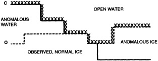
FIGURE 2a
Calculation of a representative temperature for anomalous water areas.
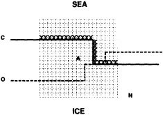
FIGURE 2b
Designation of areas near ice edge.
|
KEY: |
C |
Climatological ice edge |
|
|
O |
Observed ice edge |
|
|
X |
Boundary areas (see text). |
|
KEY: |
C |
Climatological ice edge |
|
|
O |
Observed ice edge |
|
|
A |
Target area |
|
|
N |
19° latitude x longitude area centered on target area |
|
|
X |
Climatological SSTs for these boxes are used to calculate representative temperature for area A. |
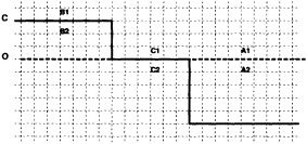
FIGURE 2c
Calculation of boundary temperatures.
|
KEY: |
C |
Climatological ice edge |
|
|
O |
Observed ice edge |
|
|
Al etc. |
1° boxes: see footnotes |
|
FOOTNOTES A. If TA2 = Temperature in 1° box A2 = - 1.8°C for observed ice, and NA1, NA2 = Normals in 1° boxes A1, A2, then TA1 = Temperature in 1° box A1 = NA1 + 0.5 (TA2 - NA2) = NA1 + 0.5 (- 1.8-NA2) B. TB2 = Representative temperature assigned to 1° box B2 (see text and Figure 2b) TB1 = NB1 + 0.5 (TB2 - NB2) = NB1 + 0.5 (TB2 + 1.8) because NB2 = - 1.8°C for climatological ice. C. TC1 = NC1 because the ice edge is at its normal position. |
|
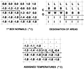
KEY TO AREA DESIGNATIONS: |
|
|
C |
Climatological ice edge |
|
O |
Observed ice edge |
|
I |
Observed ice areas set to - 1.8°C |
|
W |
Anomalous open-water areas: SSTs calculated as in text |
|
B |
Boundary SSTs: see text and Figure 2c |
|
L |
Areas left blank for filling in the Laplacian stage. |
|
FOOTNOTES A. -1.3 + 0.5 (-1.4-(-1.8)) = -1.1°C B. -0.7 + 0.5 (-1.8-(-0.8)) = -1.2°C C. -1.3 + 0.5 (-1.8-(-1.4)) = -1.5°C |
-
using ice anomaly to southward, not to westward conditions, the climatological value alone was used. If an observed SST was found in the boundary area, this was used in preference to the computed value. The SSTs in the boundary areas were then used as the external boundary conditions in the Laplacian interpolation process (Figures 2e and 2f). Reducing the ice-edge anomalies by a half had ensured that the values supplied to the Laplacian process were not extreme and had strengthened the temperature gradient at the edge of anomalously frozen areas (Figure 2f).
8. Laplacian Interpolation
-
The 1° resolution SSTs were first smoothed 1:2:1 east-west, then north-south, simplifying the smoothing to 1:1 for boxes next to land. Anomalous water areas were omitted from this smoothing, as were boundary 1° areas (Figure 2a) next to sea ice or to missing data. In this process 1° boxes adjacent to boxes still containing climatology would have been affected by the climatology, muting their anomalies. They were therefore regarded as data void, along with the boxes containing pure climatology.
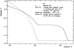
FIGURE 2e
Example of SST analysis near retreated ice edge.
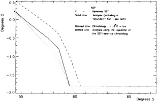
FIGURE 2f
Example of SST analysis near advanced ice edge.
-
Laplacians of the 1951 to 1980 MOHSST4 climatology (Bottomley et al., 1990) were calculated for data-void 1° boxes.
-
SSTs for the data-void 1° boxes were then computed by solving Poisson's equation with the Laplacians as forcing and the values in data-filled boxes as boundary conditions, as has been done by Reynolds (1988) and Bottomley et al. (1990) in constructing their climatology.
9. Final Smoothing
The 1° resolution absolute SST data output by the Laplacian interpolation were converted to anomalies, and the anomalies were smoothed 1:2:4:6:4:2:1 east-west, then north-south. Anomalies rather than actuals were smoothed, to avoid smoothing strong SST gradients. After smoothing, the anomalies were converted back to SSTs. SST gradients were thus retained with approximately 1° resolution, whereas the anomalies, which vary much more slowly geographically, were retained on about their original 5° resolution.
Examples of the final result of this process, in the form of anomalies for January 1878 and January 1983, are shown in Figures 1d and 3b (see color well). These fields (and others not shown) suggest that in future versions of GISST, the anomalies should be smoothed with a spatially lower-pass filter. Even in the 1980s, monthly (as opposed to seasonal) in situ SST anomalies are often unreliable on a 5° space scale (Folland et al., 1993).
INITIAL ASSESSMENT OF GISST 1.0
A sampling experiment was carried out to assess the reliability of the analysis technique when used on sparse data. In it, the complete analysis, including the Laplacian stage, was repeated for each month of the El Niño years 1982 to 1983, but with the basic SST data prior to the ''filling and quality control" stage omitted from 5° boxes where there were no data in the corresponding months of the El Niño years 1877 to 1878. In this experiment, January 1877 corresponds to January 1982, and December 1878 corresponds to December 1983. Also, data for 1981 and 1984 needed for this experiment were reduced to the coverages available in the corresponding months of 1876 and 1879. Figures 4a, b, c, and d, which should be compared with Figures 3a and b, illustrate the results of the experiment for January 1983. Figure 5a shows the two-year mean difference between the reduced-data analysis and GISST 1.0. (All are in the color well.)
Biases are largest in the eastern tropical Pacific, where the analysis of the reduced data base underestimated the strength of the 1982 to 1983 warm El Niño event. This underestimation exceeded 1°C in some places at the peak of the event in late 1982 to early 1983 (compare Figures 3b and 4d). It is likely therefore that GISST 1.0 itself will have underestimated the strength of the 1877 to 1878 El Niño, owing to the sparser data base then. Figure 5b presents the root-mean-square (rms) difference field between the GISST 1.0 and the reduced-data analyses; it is based on 24 monthly values at each location. The rms differences (which include a bias component) are less than 0.5°C over most of the Atlantic and Indian Ocean north of 40°S, but exceed 0.5°C over much of the Pacific and the Southern Ocean, and are over 1°C in the eastern tropical Pacific, where the reduced-data analyses underestimate the El Niño warmth. Cosine-latitude-weighted summary statistics for the globe and for the east tropical Pacific (20°N to 20°S, east of 170°W) are given in Table 2. The global rms difference (which also includes a bias component) is around 0.5°C before and after the El Niño but reaches 0.7°C in early 1983, when the underestimation in the east tropical Pacific averages nearly 0.7°C (compare also Figures 3b and 4d). However, the global field correlations rise from about 0.55 before the event to about 0.7 during the event and maintain this level, possibly because the El Niño intensifies the overall global anomaly pattern signal. During the El Niño the global bias reaches -0.15°C. For the two-year period as a whole, however, the global bias is only -0.03"C, suggesting, in accord with the "frozen grid" analyses in Bottomley et al. (1990) and Folland et al. (1990), that the sparse coverage available in 1877-1878 does not severely prejudice estimation of annual or multi-annual global mean SST anomalies. Similar, but apparently slightly better, results (not shown) were obtained when a corresponding experiment was made using the El Niño years 1972-1973 with the 1877-1878 coverage. The apparent improvement may have resulted from the slightly reduced coverage of observations in 19721973 relative to 1982-1983.
In a further, longer experiment the analysis for 1981 to 1990 was repeated using coverage for 1881 to 1890. Biases (not shown) were within ±0.1°C in most of the Atlantic and the Indian Ocean, and generally exceeded ± 0.3°C only in the Southern Ocean and parts of the North Pacific. Hemispheric and global average biases were within ±0.01°C. Root-mean-square differences generally exceeded 0.5°C only in the latter areas and in parts of the tropical Pacific and the far northern Atlantic. Correlations (Figure 6. again in the color well) based on 120 values at each location, exceeded 0.8 over most of the Atlantic, much of the eastern Pacific, and much of the Indian Ocean. Low correlations over the Southern Ocean and the central and northern Pacific emphasize the need to acquire more historical data for these regions.
These sampling experiments only assess the impact of reduced areal coverage of 5° box SST data. They do not provide any measure of the effects of increased scatter in the individual monthly 5° box values resulting from, for
TABLE 2 Summary Statistics for the Reduced-Sampling Test of GISST 1.0 Analysis
|
|
|
Globe |
|
|
Tropical East Pacific |
|
|
Year |
Month |
rms Difference (°C) |
Field Correlation |
Bias* (°C) |
rms Difference (°C) |
Bias* (°C) |
|
1982 |
1 |
.51 |
.57 |
-.02 |
.55 |
-.17 |
|
1982 |
2 |
.52 |
.57 |
+.01 |
.55 |
+.03 |
|
1982 |
3 |
.55 |
.55 |
-.05 |
.62 |
-.12 |
|
1982 |
4 |
.51 |
.54 |
-.08 |
.52 |
-.17 |
|
1982 |
5 |
.51 |
.57 |
-.06 |
.57 |
-.26 |
|
1982 |
6 |
.51 |
.64 |
+.00 |
.65 |
-.36 |
|
1982 |
7 |
.53 |
.63 |
+.10 |
.49 |
-.13 |
|
1982 |
8 |
.54 |
.56 |
+.06 |
.60 |
-.19 |
|
1982 |
9 |
.55 |
.67 |
+.06 |
.73 |
-.16 |
|
1982 |
10 |
.54 |
.74 |
+.01 |
.76 |
-.35 |
|
1982 |
11 |
.60 |
.70 |
-.06 |
1.09 |
-.50 |
|
1983 |
12 |
.66 |
.67 |
-.12 |
1.24 |
-.59 |
|
1983 |
1 |
.70 |
.67 |
-.14 |
1.19 |
-.63 |
|
1983 |
2 |
.69 |
.65 |
-.15 |
1.11 |
-.68 |
|
1983 |
3 |
.67 |
.65 |
-.09 |
.94 |
-.54 |
|
1983 |
4 |
.58 |
.71 |
-.03 |
.84 |
-.21 |
|
1983 |
5 |
.60 |
.71 |
+.00 |
.77 |
-.16 |
|
1983 |
6 |
.56 |
.78 |
-.09 |
.82 |
-.36 |
|
1983 |
7 |
.57 |
.78 |
-.07 |
.88 |
-.36 |
|
1983 |
8 |
.52 |
.76 |
-.05 |
.79 |
-.22 |
|
1983 |
9 |
.46 |
.72 |
-.03 |
.53 |
-.12 |
|
1983 |
10 |
.49 |
.62 |
-.03 |
.58 |
-.23 |
|
1983 |
11 |
.43 |
.72 |
+.01 |
.54 |
-.06 |
|
1983 |
12 |
.42 |
.74 |
+.02 |
.49 |
-.08 |
|
WHOLE PERIOD |
|
|
-.03 |
|
-.28 |
|
|
* Bias is "reduced-sampling analysis" minus "GISST" |
||||||
example, a smaller number of constituent observations. Also, the reduced detail of the earlier sea-ice data is ignored. To take advantage of satellite data, which are expected to improve the analyses from the 1980s onward especially in the Southern Ocean, the experiments will be repeated using GISST 1.1.
The sampling experiments on GISST 1.0 do suggest that the interpolation techniques have not introduced systematic long-term biases or false trends into the analysis. There may, however, be some systematic uncertainties owing to shortcomings in the bucket corrections resulting from the assumptions made about measurement techniques etc. (Folland and Parker, 1995). On a global average, the uncertainty arising from these is likely to be of the order of ± 0.1°C, especially before 1900 (Folland et al., 1992); but in regions where the corrections themselves are large, e.g., the Gulf Stream and Kuroshio in winter, an uncertainty of at least ±0.25°C may be expected.
A 1951-1980 monthly climatology has been created from GISST 1.0. MOHSST5 is more consistent with this than with the Bottomley et al. (1990) climatology. Relative to the latter, there were persistent anomalies of one sign in MOHSST5 in substantial parts of the Southern Ocean. These persistent anomalies were reduced or eliminated by referencing MOHSST5 to the GISST climatology. We regard the GISST climatology as the more reliable because the additional data input to GISST will have reduced the influence of the highly interpolated Alexander and Mobley (1976) climatology used by Bottomley et al. (1990) in data-sparse areas.
REVISIONS TO GISST
For GISST 1.1 we have incorporated satellite-based SSTs from R. W. Reynolds (NOAA) from 1982 onward. Because of their extensive coverage, they replaced the filling and enhancement processes, and the assignment stage except for 1° boxes adjacent to observed sea ice and Antarctica. They also almost entirely replaced the Bottomley et al. (1990) climatology in the Laplacian stage, resulting in an improved analysis. The Laplacian of the climatology was first used to make a complete field from the satellite data; then the Laplacian of this field was used to make the in situ data field complete. As expected, GISST 1.1 is warmer
in the Southern Ocean than the combined in situ satellite analysis by Reynolds and Marsico (1993), because of our different assignment of SSTs near sea ice. Typical differences are of the order of 0.5°C (see Figure 7 in the color well).
The historical in situ SST data base is to be expanded by incorporating millions of hitherto undigitized observations from the United States, Japan, and possibly the United Kingdom, Russia, and Norway. These data will also be incorporated into COADS, and an optimum data bank will be created by blending COADS and the U.K. Meteorological Office marine data base observation by observation. (See Parker (1992) as well as Komura and Uwai (1992), whose report suggests that there are about 4 million undigitized Japanese marine observations for the period 1890 to 1932.)
In collaboration with J. Walsh (University of Illinois), additional historical sea-ice data have been located and are to be digitized and combined with the Kelly (1979) sea-ice data. It is hoped that these data will be incorporated into later versions of GISST, replacing some of the existing sea-ice data.
Possible major changes to the analysis technique include:
-
Use of characteristic anomaly patterns in the background field for the Laplacian stage. The result may be an improved analysis of El Niño events in data-sparse years.
-
Refinement of the interpolation processes. The use of geographically and seasonally varying lag correlations and of optimum averaging (Gandin, 1963) is being considered.
MARINE WINDS
We are undertaking an extensive study of the dynamical consistency between sea level pressure (SLP) and near-surface wind observations in the COADS dataset. The chief motivation is the suggestion that changes in observational practice on board ships may have introduced a spurious upward trend in reported ship winds (e.g., Ramage, 1987; Cardone et al., 1990). Ward (1992) devised a method for deriving the seasonal mean geostrophic wind from COADS 2° latitude × longitude seasonal mean SLP data. A comparison of the trends in the observed winds and the derived geostrophic winds suggested a spurious upward trend in the magnitude of the observed wind of some 16 percent on average over the period 1949 to 1988. This work is being extended in two major ways:
-
Analysis is being performed on the 10° latitude X longitude (10° box) scale to improve spatial data coverage. The procedure works by first forming a 10° box anomaly data set in the way described in Ward (1992) and then adding the 10° box normal to the 10° box anomaly to get an actual value for the given 10° box.
-
A wind is derived from the 10° box grid of SLP values using a method that performs better in the tropics than does the geostrophic approximation in Ward (1992). The new method assumes a three-way balance of forces between pressure gradient, Coriolis force, and friction. The last is assumed to be linearly related to wind speed (through a constant, called the coefficient of surface resistance) and to directly oppose the wind direction. Such a system is often said to describe "balanced frictional flow," and the horizontal momentum equation can be written (see Gordon and Taylor, 1975):
where
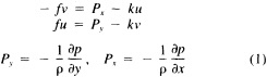
and p = surface pressure, ρ = density of air, f = Coriolis parameter, k = coefficient of surface resistance, u,v = zonal, meridional wind, and x,y = zonal, meridional distance.
Such a formulation leads to the following equations for the u and v wind components:
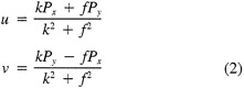
Assumptions have to be made about the value of k. It can be shown that, under the assumptions of this method, k is related to the backing angle (α) of the observed wind from the geostrophic wind:
For the studies described here, the value of k used is varied with latitude from about 2.5 × 10⁻⁵ at 50° latitude to 1.5 × 10⁻⁵ near the equator. These values are broadly consistent with the backing angle of the mean wind in directionally steady regions as calculated using climatological fields, and they are also consistent with the results of previous studies that have used other methods to estimate k (e.g., Brummer et al., 1974, Hastenrath, 1991).
To illustrate a typical result, we show time series of the December to February observed and derived u-wind component for the 10° box centered at 15°N, 45°W (see Figure 8a). The required pressure gradients are estimated as finite differences using the four boxes to the north, south, east, and west. Strictly speaking, the derived wind is applicable to a 20° latitude × 20° longitude region centered at 15°N, 45°W, so the observed zonal wind is calculated as a weighted average of the box centered at 15°N, 45°W (weight = 1.0) and the four surrounding boxes (each with weight = 0.75). The agreement between detrended versions
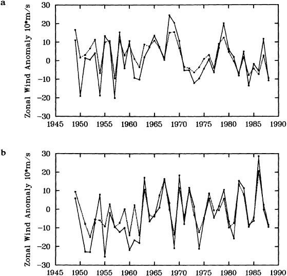
FIGURE 8
Time series of observed zonal wind anomaly (dotted line) and derived zonal wind anomaly (solid line) based on seasonal mean SLP (see Eq. 2 in text). (a) December to February for 10° latitude × 10° longitude box centered at 15°N, 45°W. (b) As for (a). but March to May centered at 55°N, 15°W. Some statistics for the series are given in Table 3.
of the derived and reported wind is excellent (Table 3, column a). This gives high confidence in the quality of the detrended component of the data and in the method used to derive the wind from the SLP. Good agreement in the detrended component of the derived and observed wind is generally found for most 10° boxes, except for some regions adjacent to the equator that show poor agreement. This is probably because Eq. 1 is less applicable close to the equator, and SLP needs to be resolved on a finer spatial scale.
The quality of the data on the longer time scale is questioned because of the difference in the trends of the two series in Figure 8a. The observed wind shows a stronger trend toward increasing wind strength than does the derived wind (Table 3). Such a result is found in most of the 10° boxes analyzed in each of the four seasons. An average spurious upward trend in the magnitude of the observed wind of about 14 percent over 1949 to 1988 is suggested by the new derived wind series. This is very similar to the value of about 16 percent derived using the different analysis scheme of Ward (1992). However, the better data coverage of the new analysis scheme is leading to the identification of a somewhat different regional pattern of biases from that in Ward (1992), which is being studied further.
One region where Ward's (1992) trend biases were substantially different from the global average was in the North Atlantic near 55°N, where the average spurious wind speed
TABLE 3 Statistics for the Wind Time Series Shown in Figure 8
|
Wind Series |
(a) |
(b) |
|
Observed Trend |
- 0.27 |
+ 0.19 |
|
Derived Trend |
-0.03 |
+ 0.40 |
|
r(O, D) |
+ 0.87 |
+ 0.89 |
|
r(Odt, Ddt) |
+ 0.94 |
+ 0.88 |
|
NOTES: Wind series (a) and (b) are those shown in Figure 8 (a) and (b), respectively. Trends are in 10 × m s-1 yr-1. For series (a), mean zonal wind is negative (i.e., easterly), so negative trend implies strengthening wind. For series (b), mean zonal wind is positive. r(O,D) is the correlation between observed wind and derived wind. r(Odt, Ddt) is the correlation after removing the linear trend from the series. |
||
change over 1949 to 1988 was suggested by the pressure data to be negative. Figure 8(b) illustrates this using the newly derived wind for March to May for the 10° box centered at 55°N, 15°W. The relationship between the observed and the derived winds seems to change around 1962. After about 1962, there is particularly good agreement between the observed and derived winds with no appreciable systematic difference in the two series. However, before about 1962, the year-to-year agreement is less good, and there is an appreciable bias; the derived wind is more easterly than the observed. This bias leads to differing linear trends in the observed and derived winds (Table 3); this difference in trends broadly supports the results of Ward (1992). Similar results are found for other nearby boxes in this and other seasons. The discrepancy before 1962 may be caused by biases in either the SLP or the wind data, or by the method used to derive the wind from the SLP data. These possibilities are to be investigated.
"CLIMATE OF THE TWENTIETH CENTURY" INTEGRATIONS
Atmospheric simulations are being commenced using the climate version of the U.K. Meteorological Office Unified Model forced with GISST 1.1. The simulations will require much-improved surface pressure and marine surface wind data sets for their verification. We anticipate substantial benefits from interactions between data analysis, modeling, and studies of the mechanisms of recent climatic variations.
ACKNOWLEDGMENTS
This work was partially supported by the Commission of the European Communities under Contract EPOC-0003C(MB), and by the U.K. Department of the Environment under Contract PECD/7/12/37.
Commentary on the Paper of Parker et al.
THOMAS L. DELWORTH
NOAA/Geophysical Fluid Dynamics Laboratory
As someone who is mostly familiar with modeling and the efforts that go into it, I am very appreciative of the tremendous effort that goes into constructing observational data sets. The data sets are of critical importance in assessing the ability of models to simulate climate and its variability. I have a few comments and a couple of examples from modeling work to emphasize the importance of the work that Dr. Parker is doing, particularly with regard to the importance of sea ice for low-frequency climate variability.
Examination of low-frequency variability contained in a multi-century integration of a coupled ocean-atmosphere model reveals that there are very long time scales associated with a number of oceanic variables in the polar latitudes of the Southern Hemisphere. In particular, there is a tremendous amount of low-frequency variability in the ice thickness, which then has a substantial impact on the model atmospheric variability. Sea ice, in some regions, can virtually disappear for times as long as a decade, with the result that surface air temperatures are much higher during this period. When you look at interdecadal model variability, features such as this are quite striking. It is critical to increase our observational data base for quantities such as sea ice in order to be able to assess whether such model features exist in the real climate system. Some of the data sets produced by Dr. Parker should help with that.
A key point in his manuscript is the theme of attempting to obtain more information from the available observations through the use of empirically motivated assumptions about the spatial and temporal scales of variations in the observed data. It is therefore critical to keep in mind when utilizing this data the assumptions that go into it. Two key assumptions are the degree of persistence in time and the spatial structure of the data. In general, this represents a powerful technique for supplementing existing data sets. There is, however, a potential for this technique to underestimate variability in data-scarce regions. This potential bias must be kept in mind.
An additional point Dr. Parker made is the critical importance of recovering and digitizing existing observations from data-poor regions. Allow me to comment on the importance of this with an additional modeling example. In characterizing low-frequency variability, a simple technique is to compute at each grid point the serial correlation of data time series. This is a measure of the persistence in the data and thus the inherent time scales. The results of such computations using annual mean sea surface temperature computed in a coupled model shows some very intriguing features. The longest time scales of sea surface temperature anomalies appear to be associated with higher latitudes where deepwater formation is occurring in the model. There are also very long time scales in the circum-Antarctic region. These are features that we would like to investigate in the observations, but the limitations in observational data sets make that difficult. For example, computing serial correlations of observed annual mean sea surface temperature from MOHSST4 produces a map with large data-void regions. In particular, the very intriguing model features in variability occur in regions with insufficient observations to assess their validity. Therefore, the technique that Dr. Parker is trying to use to extract more information from the observations available is really a critical one.
The techniques of data analysis described in the manuscript check for physical consistency between independent data. In particular, comparisons were made between derived and observed wind fields, and inconsistencies between the two were noted and studied. This is an important technique, and is an appropriate method to assess what features are real and what features are not.
Finally, as Dr. Parker mentioned, these data sets are of great utility in conducting simulations of the climate of the twentieth century. It would be beneficial to have other variables available in such a format. For example, land-surface processes might have a role in climate variability. One can envision a similar data set of time-varying land-surface characteristics over the twentieth century.
Discussion
RASMUSSON: There's much to be said for working only with real data. I hope you will also make available fields that are real data only.
PARKER: Yes, MOHSST5 is available, and we'd like to improve it by digitizing all the data possible.
KUSHNIR: If you have a good approximation to the covariance matrix structure, you can use that with more confidence than Laplacian methods to fill up missing regions.
PARKER: That would be similar to the eigenvector technique, which I think would be a good one here. We just haven't got that far yet. Also, I think getting more real data is important; for example, our pre-1953 sea ice is all from an old climatology, so the sea-ice anomalies are the same from year to year.
TRENBERTH: The use of covariances in either space or time depends very much on the nature of your signal. For instance, when you put in greenhouse warming a global-scale structure is superimposed on your fields, and larger spatial and temporal correlations are implied than you might otherwise get.
PARKER: Indeed. What would really be nice would be to have designators categorizing the quality of the data for each of the months you're presenting—for instance, with the Air Force's cloud-cover analysis, designating which are real data and which climatology.
KARL: David, when you said you tried to make the frequency of observations consistent with that of the nineteenth century, did you actually reduce the number of observations in a grid box to match the earlier ones?
PARKER: No, we had to use the box values, so we were just testing for errors resulting from the interpolation scheme. Selecting observations would have been a major computational exercise. But we are aware of that problem.
KEELING: When you are adding the COADS data to your own data set, what do you do when you have both? Can you identify the data sources and tell which are original observations?
PARKER: For the moment we are inserting the COADS SST only if the box is missing from our data set. We hope that with Scott Woodruffs help we will be able to blend the two sets, removing duplicates, by 1994. Ultimately we'd like to have everything that can be digitized.
KEELING: How hard would it be, then, to average your data by anything other than month?
PARKER: In our scheme the data are in five-day periods, or pentads, so that you could do half-months or three-month periods. We also have data sets of the bucket corrections we used so that anyone who wants to remove them from the data as they stand can do so.
JONES: We have now digitized the spring and summer months of that Danish sea-ice chart series that runs from the turn of the century to about 1960. I believe John Walsh is working on the winter ones.
WALSH: We're aggregating the narrative reports into a data set for winter. But I'd like to add that no one has yet taken advantage of the spatial character of these reports the way David has with SSTs. There is also a set of reports going back to the turn of the century from an Antarctic ice station, and some sort of spatial extrapolation procedure used on both of these might give us some measure of interannual variation in certain limited regions.
GHIL: In addition to data origin identifiers and such, I would really like to have error bars with your data.
PARKER: Well, there's a first approximation already there—the root-mean-square error fields—though they might be a lower limit, considering Tom's comment about the number of observations per grid box.
GROISMAN: I wanted to mention the dangers of using the German and Russian climatology of sea ice for the 1920s to 1940s, since sea ice was retreating considerably during this period. I hope that some day you will be able to use some Russian arctic observation data now stored in the Arctic Institute-—not digitized, of course.
LEVITUS: I'm happy to say that we at NOAA are making arrangements with the appropriate officials right now to do just that.
Decadal-Scale Variability of Ice Cover and Climate in the Arctic Ocean and Greenland and Iceland Seas
LAWRENCE A. MYSAK1
ABSTRACT
Analyses of 90 years of sea-ice concentration and ice-limit data from the Arctic Ocean and marginal seas reveal the presence of decadal-scale fluctuations in sea-ice extents, especially in the Greenland and Iceland seas. It has recently been proposed (Mysak et al., 1990) that such fluctuations may be part of an interdecadal Arctic climate cycle that can be described in terms of a reversing or negative feedback loop. An important property of this cycle is the suppression, every other decade, of convective overturning in the Iceland Sea for several winters (which occurred, for example, at the time of the "Great Salinity Anomaly" (GSA) in the 1960s, when sea-ice extents were also large). Such anomalies are preceded by increases in runoff and ice production in the western Arctic, which, it is argued, may partly cause such events as the GSA because of ice-anomaly advection from the Arctic into the Greenland Sea and subsequent ice melt in the Iceland Sea to the south. To find further evidence for this Arctic climate cycle, a lagged cross-correlation analysis of regional ice anomalies derived from sea-ice concentration data for the period 1953 to 1988 has been performed by Mysak and Power (1992). They found that both positive and negative ice anomalies in the Beaufort Sea consistently lead those in the Greenland and Iceland seas by 2 to 3 years. Mysak and Power also showed that high Mackenzie River runoffs in the mid-1980s led positive ice and negative salinity anomalies in the Greenland and Iceland seas in the late 1980s, which together resemble another (although weaker) GSA-like event.
A Boolean delay-equation model of this cycle has recently been developed by Darby and Mysak (1993). Among other things, they found that both ice and upper-ocean salinity advections from the western Arctic through to the Greenland and Iceland seas are needed in the model to create the observed structure of the Great Salinity Anomaly in the Iceland Sea.
INTRODUCTION
Over the past two decades there have been many studies of the nature and causes of interannual variability of sea-ice cover in the Arctic Ocean and marginal seas. Observational studies have been carried out by Walsh and Johnson (1979), Mysak and Manak (1989), Parkinson (1991), and others, whereas model simulations of atmospherically forced interannual variability of sea-ice extent and concentration have been performed by, for example, Walsh et al. (1985) and Fleming and Semtner (1991). Mysak and Manak (1989) also noted that the low-pass filtered areal sea-ice anomalies in the Barents and Greenland seas contain well-defined decadal-scale fluctuations, and they hypothesized that some of these might be related to the Great Salinity Anomaly (GSA; see Dickson et al., 1988), a widespread freshening of the surface waters in the subpolar gyre of the North Atlantic during the 1960s and 1970s.
In Mysak et al. (1990), hereafter referred to as M3, the decadal-scale fluctuations of ice cover in the Greenland and Iceland seas and attendant salinity anomalies in the Iceland sea (defined here as the region between Jan Mayen Island (near 71°N, 8°W) and Iceland) were further analyzed for the period 1901 to 1984, using updated Walsh and Johnson (1979) sea-ice concentration and Danish Meteorological Institute ice-limit data (Sear, 1988). In an attempt to formulate a comprehensive theory of the origin, evolution, and decay of these anomalies in the Greenland and Iceland seas, M3 linked a number of hydrological, oceanic, and atmospheric processes in the Arctic in the form of a negative feedback loop (Kellogg, 1983), which could give rise to self-sustained climatic oscillations in the Arctic for periods of 15 to 20 years. Under this scenario, GSA-like events could be regarded as cyclic rather than isolated, and as part and parcel of a sequence of complex air-ice-sea interactions.
In this paper a modified (and simplified) form of the feedback loop proposed by M3 is described, and evidence is presented for the occurrence and possible origin of another GSA-like event during the 1980s, which was predicted by M3. Because of the close relationship between salinity and sea-ice anomalies, we shall hereafter refer to these events as GISAs—great ice and salinity anomalies. Some results of a recent cross-correlation analysis (Mysak and Power, 1992), which show that sea-ice anomalies in the western Arctic consistently lead those in the Greenland Sea by 2 to 3 years, are also presented below. The question of whether GISAs have occurred prior to the 1960s is briefly addressed, and some possible links of GISAs with lower-latitude interdecadal climate fluctuations are described. (Within this context, we regard the 1960s-1970s GSA as also a GISA.)
NEGATIVE FEEDBACK LOOP FOR AN INTERDECADAL ARCTIC CLIMATE CYCLE
Figure 1 shows a six-component feedback loop of an interdecadal Arctic climate cycle that represents a modified
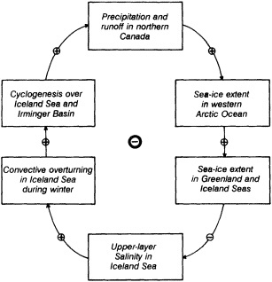
FIGURE 1
Negative feedback loop linking Iceland Sea-Irminger Basin cyclogenesis, northern Canadian river runoff, sea-ice extent, and salinity and convective overturning in the Iceland Sea (from Mysak and Power, 1992). This is a modified (and simplified) version of the ten-component negative feedback loop originally proposed by Mysak et al. (1990) to account for interdecadal Arctic climate oscillations with periods of about 15 to 20 years.
(and simplified) version of the ten-component loop in M3. The plus (minus) appearing between two boxes indicates that an increase in the first would cause an increase (decrease) in the second. Since the number of negative signs around the loop is odd, it represents a reversing or negative feedback loop (Kellogg, 1983). Therefore, in the absence of other strongly damping factors, a perturbation transferred from any one component to the next can theoretically result in a reversal of the sign of the initial perturbation. It has been estimated by M3 that the period of the climate cycle, which is twice the loop circuit time, is about 15 to 20 years.
A key feature of the loop in Figure 1 is that large negative salinity (and positive ice) anomalies in the Iceland Sea are hypothesized to be due, at least in part, to prior large runoffs from North America into the western Arctic (see the box at top of the loop). This concept of a remote forcing for anomalies like the GSA contrasts with earlier hypotheses that suggest that such anomalies are due mainly to local or neighboring atmospheric effects (Dickson et al., 1975; Pollard and Pu, 1985; Serreze et al., 1992; Walsh and Chapman, 1990a; see also the discussion in Mysak and Power, 1991). As noted in M3 (see their Figure 17), during the mid-1960s there were indeed anomalously large runoffs from North America into the Arctic and subarctic, which may have been associated with the climatic jump at that time (see
Figures 20 to 22 in M3). During the early to mid-1960s, however, the Siberian River runoffs were generally below normal (Cattle, 1985) and hence would not have contributed to a positive sea-ice anomaly in the western Arctic. The above-average North American runoffs led to large sea-ice concentration anomalies in the Beaufort Sea in the western Arctic during the mid-1960s (see Figure 19 in M3 and also Figure 3c below), which in turn were exported out of the Arctic into the Greenland and Iceland seas via the Beaufort gyre and Transpolar Drift Stream over a 2- to 3-year period (Colony and Thorndike, 1984). The melting of the large sea-ice anomalies over several summers in the Iceland Sea would then have led to the GSA, which peaked in 1968 (see Figure 6 in M3).
It is important to emphasize that the Beaufort Sea ice anomalies described above are based on ice concentration data only. As W. Chapman has suggested (personal communication), it is conceivable that during the winter and spring months, when the ice is essentially land-locked there, the ice thickness could be increasing due to the lower near-surface salinities brought about by the increased runoffs the previous summer. Such thicker ice would then be exported out of the Arctic (via the Beaufort gyre and transpolar drift stream) into the Greenland Sea, and hence add to the ice and fresh-water anomaly in the latter region. A more complete set of ice-thickness data for the Arctic (and the western Arctic in particular) may thus provide additional support for the negative feedback-loop theory.
Due to the stabilizing influence of the GSA, convective overturning during winter in the Iceland Sea, which normally brings warm Atlantic water to the surface, was suppressed, which in turn reduced the sea surface temperatures (SSTs) there (see Dickson et al., 1988). This reduction in SST, we argue, would tend to reduce cyclogenesis in this region, as well as further south in the Irminger Basin because of the advection of cold SSTs by the East Greenland Current. It is hypothesized that a lowered SST leads to reduced cyclogenesis, precipitation, and runoff over North America, and therefore causes a flip in the sign of the perturbations in the next circuit of the feedback loop. A partial confirmation of the above hypothesis has been obtained by Serreze et al. (1992), who showed that during the peak GSA years (1967-1971) the frequency of anticyclones during winter increased over northern Canada, especially over the Canadian Arctic Archipelago, which implies drier conditions in this region. Nevertheless, at this stage the link between Iceland Sea-Irminger Basin cyclogenesis and northern-Canada precipitation should be regarded with some degree of skepticism until further studies have been carried out. The idea of such a link is consistent with recent teleconnection results of Walsh and Chapman (1990b), however. They showed that winter sea level pressure (SLP) anomalies in the Iceland Sea and Irminger Basin are highly correlated (0.6 < r < 0.8) with those at the base point 75°N, 90°W in the CAA (see their Figure 12b).
Despite the above possible weakness, the feedback-loop theory has had two successful applications. First, using a cycle time of about 20 years, M3 predicted that there should be another GISA in the Greenland and Iceland seas in the late 1980s. This conjecture was verified through an examination of February sea-ice concentration data made by Mysak and Power (1991), and evidence of anomalous runoffs that might have generated this anomaly will be presented below. Second, the feedback loop in Figure 1 has been used by Darby and Mysak (1993) as a guide to developing a Boolean delay-equation (BDE) model of the interdecadal Arctic cycle. The BDE model contains six variables that represent the state of precipitation in northern Canada (1 or 0, corresponding to a high or low state), the state of ice and salinity conditions in the western Arctic and in the Iceland Sea, and the convective state in the Iceland Sea. For a variety of initial conditions, the model successfully simulates a 20-year cycle in the Boolean variables. A particularly novel result is that by allowing for different time scales for ice and salinity advection from the western Arctic through to the Greenland and Iceland seas, an ice anomaly in the Iceland Sea can persist longer than an ice anomaly in the western Arctic, a finding that is in agreement with observations.
THE 1980s GISA
Figure 2b shows that during the winters of 1987 and 1988 a large anomaly in sea-ice extent existed in the Greenland and Iceland seas, since the 0.9 ice-concentration contour extends well beyond the east Greenland coast as compared to its climatological position (Figure 2a). Concurrent with this ice anomaly, which also shows up in the late 1980s as a peak in the areal sea-ice anomaly time series for this region (see Mysak and Power, 1992), was the reduction of convection in the Greenland Sea during winter 1988 (Rudels et al., 1989) and the appearance of low-salinity water there during February and March 1989 (GSP Group, 1990). If the latter fresh-water anomaly advected southward into the Iceland Sea and suppressed convection there, then these features taken together suggest that a moderately sized GISA occurred in the Iceland Sea in the late 1980s. As in the case of the 1960s GSA, the large Greenland-Iceland sea-ice anomalies in the late 1980s appeared to have advected into the Labrador Sea by the early 1990s and thus contributed to extremely heavy sea-ice conditions and cooler air temperatures along the coast of Newfoundland in May 1991 (Globe and Mail, May 31, 1991). (It has also been argued that such positive ice anomalies off Newfoundland could be partly due to anomalous offshore winds that forced coastal ice seaward (J. Elliot, personal communication, 1991).)
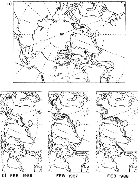
FIGURE 2
Sea-ice extent. (a) February climatology in the Arctic for the period 1953-1988. The ice concentration contours are labeled in tenths (1 indicates 0.1, etc.). In general, the sea-ice extent in the Greenland and Iceland seas is greatest during February (Mysak and Manak, 1989). (b) Monthly mean sea-ice extent in the Greenland and Iceland seas for February 1986, 1987, and 1988. While the 0.9 contour off the east Greenland coast is near its climatological position for February 1986 (see (a)), during 1987 and 1988 this contour extends well out into the Greenland and Iceland seas; in particular, it is much closer to Iceland. (From Mysak and Power, 1991; reprinted with permission of the Canadian Meteorological and Oceanographic Society.)
If the 1980s GISA is an integral part of the interdecadal climate cycle shown in Figure 1, it is conceivable that it too could have been partly generated by large runoffs in the western Arctic during the mid-1980s. Figure 3a shows that during the mid-1980s the Mackenzie River runoff was indeed slightly above average. This led to below-average salinities on the Beaufort shelf to the north of the Mackenzie delta (Figure 3b) and, for the period 1984-1986, to above-average areal sea-ice anomalies (Figure 3c) in the western Arctic subregion B1 (identified in Figure 4). Heavy ice conditions in the Beaufort Sea can also be seen at this time in the ice atlas of Mysak and Wang (1991) (see also Figure 4b
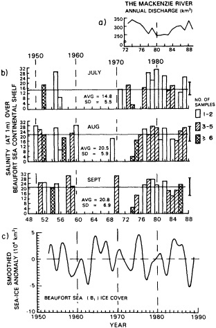
FIGURE 3
(a) Annual Mackenzie River runoff at the Arctic Red River (a city on the Mackenzie River) for 1973-1989 (data courtesy of R. Lawford). (b) Salinity at I m depth over the southeastern Beaufort Sea continental shelf (in subregion B1, shown in Figure 4) in July, August, and September for 1950-1987 (data from Fissel and Melling, 1990). (c) Smoothed areal sea-ice anomalies in the Beaufort Sea subregion B for 1953-1988. (From Mysak and Power, 1992; reprinted with permission of the Canadian Meteorological and Oceanographic Society.) In deriving the time series in (c), the monthly areal sea-ice-extent anomalies were low-pass filtered so as to remove all fluctuations with periods shorter than 30 months.
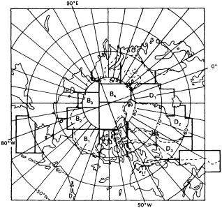
FIGURE 4
Subregions used in the cross-correlation analysis of low-pass filtered sea-ice anomalies derived from ice-concentration data given on a 1°X 1° (latitude) grid (developed by Walsh and Johnson, 1979) for 1953-1988. (Adapted from Mysak and Power, 1992; reprinted with permission of the Canadian Meteorological and Oceanographic Society.) In this paper cross-correlation results are presented only for the subregions labeled B1, B2. B3, B4, D1, D2, and D3. The dashed line denotes the 200 m isobath.
in Mysak and Power, 1992). It is also interesting to note the sharp ice-anomaly peak in 1975, evident on Figure 3, which presumably occurred in response to the high runoff and low salinities in 1974; similarly, we note the sequence of low ice anomalies from 1978 to 1982, which correspond to low runoff and high shelf salinities at that time. Figure 3c also indicates the large ice anomalies from 1964 to 1967, which, as was pointed out by M3, were likely due to the very large runoffs in 1964-1966. (Mysak and Power (1992) present evidence that shows that local winds may also have played a role in producing the Beaufort Sea ice anomalies.)
It has often been suggested by critics of the interdecadal-cycle theory characterized by Figure 1 that runoff from the Siberian rivers, which in total is 4 to 5 times that of the Mackenzie, should contribute substantially to sea-ice anomalies in the Arctic and subsequently in the Greenland and Iceland seas. Here we counter (as does M3, in more detail) that, because the Eurasian shelf is very wide and shallow, this runoff gets well mixed there with the central Arctic Ocean waters that also flow onto the shelf. Such mixing takes place mainly through tides and eddies in this region; also, convective overturning on the shelf mixes the surface runoff with the deeper shelf water. Fluctuations in the Siberian river flow thus have little direct bearing on the creation of sea-ice anomalies in the central Arctic. A similar conclu-
sion was also reached by Ikeda (1990), who considered effects of runoff on sea ice in the Barents Sea.
CROSS-CORRELATION ANALYSIS OF SEA-ICE ANOMALIES IN THE WESTERN ARCTIC AND GREENLAND SEA
To verify that sea-ice anomalies produced in the Beaufort Sea are advected into the Greenland and Iceland seas in 2 to 3 years' time (as proposed in the feedback loop), we first grouped according to subregion the monthly sea-ice concentration data (Walsh and Johnson, 1979) that had been collected on a square 1° × 1° (latitude) grid for the period 1953-1988. Figure 4 depicts these subregions; B1 to B4 are in the Beaufort Sea and Canada Basin, and D1 to D3 are in the Greenland, Iceland, Irminger, and Labrador seas, the latter two seas being source regions of North Atlantic Deep Water. Then a monthly time series of the areal sea-ice anomalies was computed for each subregion (i.e., the concentration departure from the long-term mean for each month at a grid point in the subregion was multiplied by the grid area). The procedure is similar to that followed by M3, who studied the advection of Greenland Sea ice anomalies into the Labrador Sea via five subregions (see Figures 2 and 3 in M3). The monthly time series for each subregion was next low-pass filtered to eliminate high-frequency components, i.e., those periods shorter than 30 months. (A description of the filtering process can be found in Power and Mysak (1992).) An example of one such low-passed time series is shown in Figure 3c.
Note that the subregions B1 through B3 were chosen to follow the Beaufort gyre ice-drift pattern in the deep part of the Arctic Ocean, so that the anomaly advection would not be contaminated by smaller-scale ice motions on the Eurasian shelf. The lagged cross-correlation functions for the low-passed fluctuations in B1 versus those in the other subregions were computed and examined for asymmetries about zero lag (e.g., as seen in Figure 4 of M3). The maximum lagged correlation coefficients obtained from this analysis are given in Table 1. To find the 95 percent significance level for the correlations, the number of degrees of freedom (for simultaneously correlated data) was estimated to be 2N/30 = 29, where N = 432 (total number of points of data). Then from Table 13 in Pearson and Hartley (1966), we obtained, using a one-tailed test for normally distributed data, a 95 percent significance level of r = 0.3. For lagged cross-correlations, the estimated number of degrees of freedom decreases with lag; the 95 percent significance level for the correlation coefficient r, which is estimated to be 0.3 for simultaneously correlated data, slowly increases to 0.36 for a lag of 120 months.
The results in Table 1 show that the low-pass filtered sea-ice anomalies in B1 lead those in the Greenland Sea (subregion D1) by just over 2 years, and, moreover, that there appears to be a continuous advection of ice anomalies by the Beaufort gyre, the Transpolar Drift Stream, and the East Greenland Current all the way into the Labrador Sea. (Although the maximum cross-correlations for B1 versus D2 and D3 are not significant at the 95 percent level, the correlations between data from adjacent regions are significant (Mysak and Power, 1992) and support the above conclusion.) Chapman and Walsh (1991) found that (unfiltered) monthly Beaufort sea-ice anomalies also led those in the Greenland Sea (see their Figure 12); however, they did not estimate the time lag involved nor did they carry out an analysis of the sea-ice fluctuations between subregions B1 and D1. A detailed discussion of the sea-ice anomalies described here, and also of those in the other subregions shown (but not labeled) in Figure 4, is given in Mysak and Power (1992). The possible role of wind forcing in creating these anomalies is examined by Mysak and Power (1992) as well.
To estimate the average advection speed of the anomalies from the Beaufort Sea into the Greenland Sea and beyond, a cumulative lag plot was constructed (Figure 5). From the best linear fit to the data, we find an average advection speed of about 2000 km/yr, or roughly 5 km per day, which lies well within the range of typical drift speeds for sea ice, namely 1 to 10 km per day (Chapman and Walsh, 1991).
EVIDENCE FOR EARLIER GISAs
In M3 the ice-limit data of the Danish Meteorological Institute (DMI) for the period 1901-1956, which give the summer ice-edge positions in the Greenland, Iceland, Irminger, and Labrador seas, were analyzed for evidence of earlier GSA-like events. It was noted that in response to large North American runoff increases in 1931-1932 and 1945-1947 (see Figure 17 in M3), the sea-ice extent in the Greenland and Iceland seas increased noticeably a few years
TABLE 1 Maximum Lagged Correlation Coefficients (r) for Smoothed Areal Sea-Ice Anomalies in Subregion B1 (see Figure 4) Versus Those in Other Subregions, with the Lag at Each Maximum Correlation
|
|
B2 |
B3 |
B4 |
D1 |
D2 |
D3 |
|
rmax (with B1 leading) |
0.27 |
0.33 |
0.53 |
0.40 |
0.27 |
0.21 |
|
lag (months) at rmax |
2 |
5 |
28 |
27 |
36 |
39 |
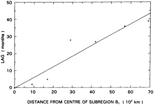
FIGURE 5
Best linear fit to the lag at maximum cross-correlation (taken from Table 1) versus distance from center of subregion B1 to center of subregion D3 via the centers of subregions B2, B3, B4, D1, and D2 shown in Figure 4. (From Mysak and Power, 1992; reprinted with permission of the Canadian Meteorological and Oceanographic Society.)
later (see Figure 15 in M3), in agreement with the right-hand side of the feedback loop in Figure 1. Moderate peaks can also be seen in the annual Koch ice index (the number of weeks per year that ice affects the coast of Iceland) at about the same time as the large ice limits, namely, around the early 1930s and late 1940s (Figure 10 in M3). Mysak and Power (1991) showed that the North American runoff in Figure 17 in M3 (a 38-year time series) leads the Koch ice index by 3 to 5 years, which provides further evidence of the correlation between runoff and sea ice implicit in the feedback loop. (The above lag correlation has also been recomputed (R. Tyler, personal communication, 1992) using a 50-year runoff record (1918-1967); it was again found that the runoff leads the Koch ice index by about 5 years.)
More recently, the spectrum of the Koch ice index for the period 1600-1970 has been computed by Stocker and Mysak (1992) in their analysis of high-resolution proxy data from the Holocene epoch. As well as a peak at around 90 years, they found significant energy at 27 years (see their Figure 10), which corroborates the finding of such a signal in a previously computed Koch ice-index periodogram using a shorter time series (Figure 25 in M3). This 27-year peak is also remarkably close to the 24-year peak in the spectrum of the central England temperature record (Stocker and Mysak, 1992) and also to the 20-year oscillation seen in the Greenland ice-core oxygen-isotope records, which extend over a 700-year period in the recent Holocene (Hibler and Johnsen, 1979). In view of the latter results, other ice-core data from glaciers in the Canadian high Arctic should be examined for evidence of interdecadal climate oscillations. From very short ice cores extracted from the Devon ice cap, F. Koerner (personal communication, 1992) found evidence of large accumulations in the mid-1960s, which is consistent with the sudden precipitation increase that was observed at that time in the Canadian high Arctic (Bradley and England, 1978). Thus the analysis of longer, high-resolution ice cores from the Canadian north could be quite revealing from the viewpoint of Arctic interdecadal variability.
POSSIBLE CONNECTIONS OF GISAs WITH LOWER-LATITUDE INTERDECADAL CLIMATE VARIABILITY
We shall divide the discussion on this issue into three parts:
-
We could suppose (perhaps naively) that the interdecadal Arctic climate cycle described in this paper is essentially self-contained (like some theories of ENSO, which involve air-sea interactions in only the tropical Pacific region) and is thus independent of lower-latitude variabilities. This assumes, for example, that the variability of Pacific inflow through the Bering Strait is unimportant, that exchanges between the Arctic Ocean and the Canadian Arctic Archipelago have little effect, and that atmospheric interdecadal fluctuations in lower latitudes essentially peter out in the Arctic.
-
Even if the above is essentially correct, it is nevertheless conceivable that the Arctic climate cycle could induce interdecadal variability at lower latitudes.
-
Alternately, lower-latitude interdecadal variability in the climate system (and in the ocean in particular) may very well have an influence on or trigger some aspects of Arctic interdecadal variability. We will expand on the second and third possibilities below.
The Arctic as a Trigger for Lower-Latitude Fluctuations
One way in which the interdecadal Arctic cycle could influence lower-latitude climate is through the connection between the Arctic Ocean and the Greenland Sea via Fram Strait. According to Aagaard and Carmack (1989), because the waters in the Greenland Sea are weakly stratified, they are ''delicately poised with respect to their ability to sustain convection," and therefore the latter process is sensitive to the amount of fresh water exported from the Arctic. A modest increase in this water supply could severely reduce convection in the Greenland Sea. However, it is not believed (R. Dickson, personal communication, 1992) that this reduction in convection occurred during the time of the GSA. It is also conceivable that alternating periods of heavy and light Greenland-Iceland sea-ice anomalies, which are accompanied by relatively cold and warm upper-ocean tem-
peratures respectively (see Figure 6 in M3), could result (via advection) in decadal-scale SST anomalies in the southwestern part of the subpolar gyre a few years later, an idea proposed by Mysak (1991). For example, our Figure 6, which depicts the SST anomalies averaged over 45°N to 55°N in the Atlantic Ocean, clearly indicates the existence of alternating cold and warm periods in the northwestern Atlantic, i.e., at around 30°W. To the left of the time axis is a sequence of solid and dotted lines that indicate heavy or light ice conditions, respectively, in the Greenland and Iceland seas. In several cases, we observe that heavy ice conditions precede negative SST anomalies in the northwestern Atlantic by approximately 5 years (the advection time from the Greenland and Iceland seas to this region); similarly, light ice conditions in the Greenland and Iceland seas precede positive SST anomalies, also by about 5 years. While the correspondence between heavy (light) ice conditions and warm (cold) SST anomalies in the northwestern Atlantic is not completely one-to-one, the relationship is sufficiently encouraging to warrant further investigation and increased monitoring of high-latitude climate parameters.
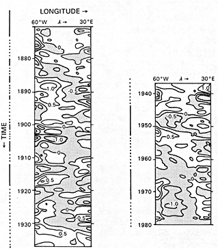
FIGURE 6
Low-pass filtered and detrended sea surface tempera- ture anomalies averaged over the latitude band 45°N to 55°N as a function of time and longitude in the North Atlantic and Baltic Sea. (Adapted from Bryan and Stouffer, 1991; reprinted with permission of Elsevier Scientific Publishers.) Solid and dotted lines on the time axis indicate, respectively, periods of relatively large and small (or near-normal) sea-ice extents in subregion D1 (see Figure 4) of the Greenland and Iceland seas, as estimated from the sea-ice data described in Figures 3, 10, and 15 of Mysak et al. (1990).
A second way in which Arctic sea-ice changes could induce climate variability at lower latitudes is via the surface albedo: Anomalously large sea-ice extents increase the albedo, and vice-versa. However, the change in the area covered by the sea ice that can be ascribed to natural decadal-scale variability is only of the order of a few percent; such variations are therefore unlikely to induce changes in the polar energy budget large enough to affect the lower latitudes via atmospheric circulation. The Southern Hemisphere sea-ice cover, however, may show larger changes on the interdecadal time scale, in which case Arctic albedo changes and climate need to be discussed together with the natural variability of the southern polar region.
The possibility that polar (in contrast to just Arctic) and high-latitude climate fluctuations on decadal time scales may be related, with the former driving the latter, is suggested by the spatial structure of the third empirical orthogonal function of SST that has been computed by Folland et al. ( 1986a). (For a clear picture of this EOF, which accounts for 6 percent of the SST variance, see Figure 2 in Bryan and Stouffer (1991).) The largest amplitudes of this EOF, whose temporal fluctuations have an interdecadal time scale, are in the northeast Pacific, the northwest Atlantic, and a broad range over the South Atlantic and South Indian oceans. (Folland et al. (1986b) have shown that this EOF is closely linked with Sahel rainfall.) At the same time, we note that because of the particularly large SST gradients in the northeast Pacific and northwest Atlantic, it is conceivable that this EOF's variations may be driven by interdecadal variability in the Arctic. A recent study by Walsh and Chapman (1990b) showed that monthly Arctic SLP fluctuations in winter are associated with or teleconnected to SLP changes in the northern North Atlantic. In a continuation of this study, using data from all seasons, Power and Mysak (1992) showed that at low frequencies (periods of 5 years and longer) this teleconnection pattern persists; in addition, they found that at low frequencies another teleconnection pattern exists between centers in the Arctic and the North Pacific. However, neither of these studies addresses the question of cause and effect, so this information should be taken mainly as a starting point for further work on determining how the polar regions (and the Arctic in particular) drive lower-latitude fluctuations.
Lower-Latitude Forcing of Arctic Fluctuations
The third viewpoint noted earlier, namely, that lower-latitude interdecadal fluctuations trigger Arctic climate fluctuations on this time scale, perhaps has the most widespread appeal. There have been many recent observations of interdecadal variability at middle and tropical latitudes in the climate system (for a list of references, see Weaver et al., 1991). Many investigators believe that these fluctuations may be due to internal oscillations in the thermohaline
circulation—an idea that appears to originate with Bjerknes (1964), and one that has also been developed by many ocean modelers (see, e.g., Weaver et al., 1991; Delworth et al., 1993). This meridional overturning circulation is global, and transports heat from low to high latitudes. Thus, changes in this transport would produce high-latitude changes in the atmospheric surface temperatures at locations where the thermohaline circulation "ventilates" (in the North Atlantic and in the Southern Ocean). Such changes in the poleward heat transport in the North Atlantic have recently been observed by Greatbatch and Xu (1992). Furthermore, such changes in the heat transport could have produced the type of SST anomalies seen in Figure 6. In particular, Greatbatch and Xu found increased transports (at 54.5°N) in the 1950s and reduced transports in the 1970s, which correspond to the warm and cold SSTs seen at these times in Figure 6.
The influence of the aforementioned SST anomalies on the atmospheric circulation has been studied by Peng and Mysak (1993), among others. They showed that during the warm 1950s there was a teleconnection pattern of high-low-high sea level pressure centers established across the North Atlantic, Europe, and western Siberia. During the cold 1970s, however, there was a very large low-pressure system extending from the North Atlantic to central Europe. These two circulation patterns in the atmosphere had very different effects on the precipitation and runoff over western Siberia. Peng and Mysak found that during periods of warm SST anomalies there tended to be less precipitation and hence less runoff into the Arctic, whereas during the cold years there was more precipitation and runoff into the Arctic. One important conclusion from this study is therefore that the fresh-water budget in the Arctic is indeed affected by lower-latitude interdecadal fluctuations in the ocean. However, it does not appear that the induced changes are directly related to the interdecadal Arctic climate cycle, because the runoff into the Siberian shelf does not seem to have an immediate effect on sea-ice concentration in the central Arctic.
In a recent study by Higuchi et al. (1991), it was shown that the standing-eddy poleward heat transport in the lower troposphere in the Northern Hemisphere exhibits strong decadal-scale variability. In particular, in years of very large or very weak transports, the ice margin in the Greenland Sea is substantially reduced or expanded accordingly. Thus in this case the atmosphere is a medium that can transmit interdecadal signals into the Arctic region and possibly influence the sea-ice cover.
While many of the above suggestions are rather speculative, we believe it worthwhile to look further at connections between middle- and polar-latitude interdecadal variabilities in the climate system. In particular, we should examine the Southern Ocean and Antarctic regions for interdecadal variability to see whether there are any manifestations (e.g., ice anomalies) similar those found in the Arctic. However, one should bear in mind that if these northern and southern variations are linked by the influence of the thermohaline circulation, there will be long time lags (of the order of a hundred years) between related events in the two polar regions, because the overturning time scale of the thermohaline circulation in the Atlantic basin is a few centuries (see, e.g., Mysak et al., 1993). Also, another important factor that should be kept in mind is the different geographies of the two polar regions: The Arctic Ocean is surrounded by a land mass, whereas the Southern Ocean surrounds the Antarctic continent.
In conclusion, it perhaps is worth making one final point, which concerns both polar regions as well as the lower latitudes. It can be summed up colloquially as follows: "What sea surface temperature is to interannual variability in the tropics, sea surface salinity is to interdecadal variability at high latitudes." This contrast arises because of the very different effects of SST and sea surface salinity anomalies on the atmosphere, a relation well known to ocean and climate modelers (Weaver et al., 1991). Air temperature responds fairly quickly to changes in the sea surface temperature (on time scales of the order of weeks to months), whereas precipitation is not so immediately affected by surface salinity changes. There can be feedbacks to the atmosphere through the hydrological cycle, ocean circulation, and sea-ice formation, drift, and decay, but, as described in this paper, they are on time scales of the order of decades.
ACKNOWLEDGMENTS
The author is grateful for financial support received over the past several years from the Canadian Natural Sciences and Engineering Research Council, the Canadian Atmospheric Environment Service, Fonds FCAR (Québec), and the U.S. Office of Naval Research. It is also a pleasure to thank Ann Cossette for typing the first draft, John Walsh for helpful discussions, Douglas Martinson for his interest in and review of this paper. The comments of Bill Chapman on an earlier draft of this paper are gratefully acknowledged.
Commentary on the Paper of Mysak
DOUGLAS G. MARTINSON
Lamont-Doherty Earth Observatory
I want to start by commending Dr. Mysak for attempting to combine a wide variety of observations and processes into a single feedback model. Having said that, I want to play a "friendly devil's advocate." First, as you point out, there is a decrease in the Siberian river runoff into the Arctic that coincides with an increase in the Mackenzie River runoff. What is the net effect of that sort of competition?
That leads to the next point, the influence of runoff on ice growth. Are you suggesting that the runoff influences the ice growth through its impact on stability? If so, is the Beaufort Sea less stable than the region receiving the Siberian river inflow? Or are you suggesting some other mechanism? Alternatively, might the increased runoff be indicative of some other atmospheric anomaly (e.g., winds, temperature, cloud cover) that more directly affects the ice cover? Also, do you know whether the increased areal distribution of ice actually represents more fresh-water? Spreading of the ice in the Greenland Sea by increased winds would also lead to thinner ice, in which case the net volume of fresh-water has not necessarily changed.
Now for some general points. You suggest that local convection changes the SST, which in turn influences the cyclogenesis. As Walter Munk asked previously, can the small spatial scales of convection significantly influence SST? In other words, how exactly do you envisage the convection's influencing SST to the extent that it could affect cyclogenesis? Might not the lateral influences be more important? Also, if the cyclogenesis in the Greenland Sea is increased, it is still difficult for me to imagine that it drives increased precipitation so far to the west.
Finally, a comment regarding the shutdown of convection in response to an increase in advected sea ice (fresh-water). I just want to point out that in the Weddell Sea today, a large output of glacial ice from the Filchner, Ronne, and Larson ice shelves is streaming ice down the eastern side of the Antarctic peninsula, and that is the region where we have the largest source of Antarctic bottom water. If you track this ice, it reenters the Weddell in the vicinity of the Greenwich meridian where the open ocean convection was observed in the mid-1970s. Therefore, the relationship between advected ice and a convection shutdown must not be as straightforward as it might otherwise seem.
Those are a few interesting lead-in points, and I appreciate the model you have given us to talk about.
Discussion
GROISMAN: As I remember, 70 to 80 percent of the fresh-water input into the Arctic from Eurasia comes from rivers, some of which are highly variable in volume. You would have to take that variability into account in that region.
MYSAK: The tremendous mixing due to tides and even convection on the wide continental shelf in the Arctic Ocean that borders Eurasia seems to minimize Eurasian runoff water's impact on sea ice. In the Beaufort Sea region, where the shelf is very narrow, there seems to be an immediate effect.
MOREL: One must be careful not to interpret an association of anomalies, even if it occurs more than once, as a causal relationship, particularly when it involves precipitation. The models tend to yield different anomalies.
TRENBERTH: If sea ice melts, it creates fresh-water that substantially affects salinity. But I believe that observational evidence suggests that you get more ice created because it's cold than because the water is fresher.
MYSAK: For a given air temperature you'll get more ice if the water's fresher. Also, some data I looked at didn't show a very good correlation between cold-air temperature anomalies and sea-ice formation, but then it was limited to spring and summer.
LEHMAN: I'd like to comment on topics from the last several presentations. First, Bob Dickson said that he didn't feel the net overflow in the Greenland/Icelandic/Norwegian Sea area was being affected—in other words, that its strength was invariant on, say, decadal time scales. It seems to me that the topographic barrier acts to filter out variability there on short time scales. I should note, however, that I disagree with him about the short-time-scale stability of the thermohaline circulation.
Now let's consider some consensus views on the relative transports for the two different limbs of the North Atlantic Deep Water: overflow water and the Labrador Sea water (ignoring recirculation). You might have about 6 sverdrups for the former, and 7 to 8 for the latter, which is not insignificant. Together they constitute a potent climate forcing agent.
If the modelers can get the deep-water formation north of the
ridges right, we can explore the sensitivity of these limbs to the same kind of salinity forcing. I predict that the Labrador Sea limb will respond on short time scales, and represent an important effect on the thermohaline circulation.
RIND: It has been suggested that at the time the last glacial cycle started there might actually have been a shutoff of the GIN seas component, while the Labrador Sea component continued.
GHIL: If North Atlantic Deep Water is formed by Arctic intermediate water, we need to know what controls the formation of the Arctic intermediate water so we can put it into our models.
LEHMAN: The convection and water formation at both levels seem to be responding to salinity forcing at the surface, but even if the forcing fails to drive convection there's enough water backed up behind the sills to keep overflowing. I know I've simplified by ignoring the wind-driven gyre, but things might be simpler in the Labrador Sea. It would be interesting to apply the same salinity forcing to it as to the Norwegian Sea, and see whether you get the climate vibration you might expect.
GROOTES: This morning almost everyone said that we have some evidence for a 10- or 20-year time scale change, but not a long enough record. I just wanted to mention that my Figure 4 definitely shows a fluctuation on that scale. The Greenland ice sheet serves as a high-resolution monitor for climate variability in the Greenland and North Atlantic area, and I think we ice-core people need to get together with the oceanographers and modelers to put this kind of proxy data to better use.
Long-Term Sea-Level Variation
BRUCE C. DOUGLAS1
ABSTRACT
Published values for the long-term, global-mean sea-level rise determined from tide-gauge records range from about 1 to 3 mm per year. I have argued (Douglas, 1991) that the scatter of the estimates appears to have arisen from use of data from gauges located at convergent tectonic plate boundaries or affected by land subsidence or uplift due to isostatic rebound from the last deglaciation, and especially data reflecting the effects of large interdecadal and longer sea-level variations on short (850 years) records. Using only long and nearly complete records from locations where tectonic plates do not collide, and correcting for rebound with the Tushingham and Peltier model (1991), I obtained for 21 stations in nine oceanic regions during 1880-1980 a value of 1.8 (±0.1) mm/yr for global sea-level rise. Because low-frequency signals in the sea-level record even more seriously affect estimates of acceleration, I examined (Douglas, 1992) the longest tide-gauge records for evidence of a past, globally coherent, nonlinear component of sea-level rise. For the 80-year period 1905 to 1985, 23 essentially complete tide gauge records in 10 geographic groups were found to be suitable for analysis. These yielded an apparent global acceleration of -0.011 ( ± 0.012) mm/yr2. A larger, less uniform set of 37 records in the same 10 groups, having an average length of 92 years and covering the 141 years from 1850 to 1991, gave a value of 0.001 (± 0.008) mm/yr2. Thus there is no evidence for an acceleration in the past 100 + years that could be termed significant, either statistically or by comparison with the value (0.15 to 0.2 mm/yr2) predicted to accompany global warming. The large interdecadal fluctuations of sea level so severely affect estimates of regional and global sea-level acceleration for time spans of less than about 50 years that future tide-gauge data alone cannot serve as a leading indicator of climate change. If the interdecadal fluctuations of sea level could be understood in terms of their forcing mechanisms and removed from the records, then tide-gauge data would be useful over shorter spans.
INTRODUCTION
Concern over the consequences of global warming has inspired many examinations of historical tide-gauge records to determine the rate of sea-level rise. Excellent summaries of the sea-level-rise problem are available in the National Research Council's Sea-Level Change (NRC, 1990) and the Intergovernmental Panel on Climate Change's report Climate Change: The IPCC Scientific Assessment (IPCC, 1990). Interest in sea-level rise is high due to its obvious practical impact, and because of its scientific value as an indicator of global change. In the latter respect, global sea level is similar to earth orientation (Carter et al., 1989). Both give measures that are necessary (but not sufficient) conditions for evaluating model predictions.
Published values for global sea-level rise for the last 50 to 100 years vary from about I to 3 mm/yr (Barnett, 1990), with formal uncertainties ranging from 0.15 to 0.90 mm/yr. While there is not much doubt that sea level is rising, the scatter of results makes impossible a meaningful interpretation of the global balance of water in its various forms and locations.
The large disparity of results arises in part (Barnett, 1990) because authors analyze data in different ways, and select and group tide-gauge stations according to different criteria. Emery and Aubrey (1991) have pointed out in addition the importance of vertical crustal movements on estimates of sea-level rise. Also, Pugh (1987) and Munk et al. (1990) noted the importance of decadal variations, and Sturges (1987) further warned of the influence of very-low-frequency variations of sea level on estimates of sea-level rise. To minimize these latter problems, I selected or rejected sea-level time series from tide gauges (Douglas, 1991) according to length and completeness of record, general agreement with other nearby stations over a common time interval, and freedom from obvious tectonic effects. Stations were grouped according to oceanic region. The station groups surviving this selection process formed an extremely consistent set, particularly after correction for the effects of post-glacial rebound (PGR) by the ICE-3G model of Tushingham and Peltier (1991). In fact, the rms difference of sea-level rise data for widely separated oceanic regions from long records exceeding 60 years in length, after correction for PGR, was so good (0.4 mm/yr) that the data could be aggregated without regard to record length. This obviated the need for statistical methods such as empirical orthogonal function (EOF) analysis. The value I obtained (Douglas, 1991) for the global (linear) sea-level rise was 1.8 mm/ yr ±0.1. The small value of the uncertainty reflects the consistency of sufficiently long records.
Woodworth (1990) and Douglas (1992) have further considered the question of an acceleration of global sea level. Using somewhat different approaches, both concluded that there is no evidence of a statistically significant acceleration (i.e., quadratic variation) of global sea level over the past century. However, these authors differed considerably in their views of how quickly a regional or global acceleration of sea level could be detected in future tide-gauge records. Woodworth concluded that a regional acceleration could be confirmed at the 95 percent confidence level within a few decades. Douglas was far more pessimistic, because of the chaotic occurrence of large and durable low-frequency sea-level variations in the records.
THE SEA-LEVEL RECORD
The IPCC report gives for the "business as usual" scenario of global warming an additional sea-level change of 18 cm by the year 2030 and 44 cm by 2070, corresponding to accelerations of about 0.22 mm/yr2 in the former case and 0.14 mm/yr2 for the latter (IPCC, 1990). Verification of these or similar predictions at an early date is necessary in order to establish confidence in climate models and forecasts.
Determinations of sea-level acceleration suffer from the same problems as determinations of linear sea-level-rise value, with an important exception, viz., steady vertical crustal movements. The most pervasive of these, post-glacial rebound, is linear over the time span for which tide-gauge data are available (Peltier and Tushingham, 1989) and is of no consequence in computation of the acceleration in a record. Any other temporally linear vertical crustal movement, such as that associated with colliding tectonic plates at places with long earthquake-recurrence times, is similarly not a factor. As a result, many more tide-gauge records are usable for an analysis of apparent global sea-level acceleration than for determining the linear trend.
Although data from more gauges are available for analysis of apparent sea-level acceleration than for the case of the linear rise, this is of little significance. The reason is that at low frequency, spatial coherence of sea level is very great. Thus a region such as the Baltic, which contains a score of long records, is effectively a single measurement system for examining decade-to-century-scale and longer sea-level variations. Figure 1 illustrates this phenomenon. The data are monthly mean values of sea level from the Permanent Service for Mean Sea Level (PSMSL) (Spencer and Woodworth, 1991) that have been detrended over the common time period 1895 to 1965 and smoothed by a Gaussian filter with full width at half maximum of four years. Five typical sea-level records, in ascending order from the southernmost part of the Baltic northward to Stockholm and then well eastward into the Gulf of Finland, are displayed. These low-pass filtered records are striking for their spatial and temporal coherence and the long relative
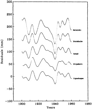
FIGURE 1
Detrended and low-pass filtered sea-level records in the Baltic. Note the extraordinary coherence at low frequency.
decline from about 1925 to 1940. This low-frequency "noise" corrupts a determination of acceleration from these records, and is clearly not independent from one site to another. Such large and persistent oscillatory sea-level events, present in most tide-gauge time series, radically affect the value of apparent sea-level acceleration derived from records even many decades in length. Figure 2 shows that even a near-100-year record may not be long enough to obtain a representative sample of low-frequency sea-level variation at a site. It presents the filtered and detrended sea-level records for Nedre Sodertalje and Stockholm, sites only about 25 km apart that have records nearly the same length, at just over 90 years. The difference between them is that the Nedre Sodertalje series covers an earlier period, before the Stockholm record began, but one that exhibited a large, persistent sea-level variation comparable in amplitude to the event of 1925 to 1940.
Such large and enduring sea-level variations are not unusual in tide-gauge records. Figure 3 shows the filtered and detrended record for San Francisco, the longest continuous record available for the United States. Clearly visible are interdecadal fluctuations as well as larger, lower-frequency oscillations. These signals obviously corrupt determinations of rise and acceleration. Figure 4 shows the results for the linear rise at San Francisco computed from the original unfiltered monthly mean values for a sliding 30-year win-
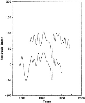
FIGURE 2
Low-pass filtered and detrended records for Stockholm (top) and Nedre Sodertalje (bottom).
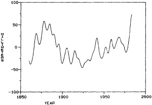
FIGURE 3
Low-pass filtered and detrended sea levels for San Francisco. Note the existence of very large low-frequency signals in the record.
dow. The 30-year linear rise value at San Francisco varies from +5 to -2 mm/yr over the record. Figure 5 presents the acceleration estimates (in mm/yr2) for the same sliding 30-year window. These values are, of course, even more variable than the linear term values, ranging from + 0.5 to -0.5 mm/yr2. Clearly, determining a meaningful global acceleration value requires using a well-distributed set of oceanic regions that lack interregional coherence.
REGIONAL AND GLOBAL SEA-LEVEL ACCELERATION
In the Douglas (1991) paper on global sea-level rise, the condition was enforced that all records used had to be about 80 percent or more complete because of the presence of low-frequency sea-level variations. From the comments above, it is clear that the apparent acceleration determined for a site can also be affected by a data gap, so the same condition needs to be applied for an analysis of acceleration.
As we have seen, record length is a critical parameter in the selection of data sets. Figure 6 displays quantitatively how record length affects the apparent acceleration estimate by displaying it as a function of data span for PSMSL records more than 10 years long. The scatter of accelerations for record lengths less than about 40 to 50 years is very
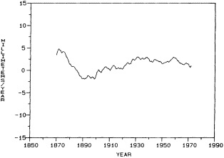
FIGURE 4
Sea-level rise in mm/yr for San Francisco, for a sliding 30-year window of the original monthly mean values.
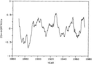
FIGURE 5
Apparent sea-level acceleration in mm/yr2 for San Francisco, for a sliding 30-year window. The amplitude of the low-frequency excursions is about twice the value anticipated to result from future global warming.
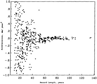
FIGURE 6
Apparent accelerations of sea level for records more than 10 years in length. Low-frequency variations of sea level heavily corrupt the computation of an acceleration parameter for records less than about 50 years in length.
great; the reason for the striking increase in consistency beginning with records over 50 years long is unknown. Of course, the scatter of shorter records in Figure 6 is due to absorption of interdecadal variability into the estimate of acceleration. The figure clearly shows the site dependence of apparent sea-level acceleration, even for records that are many decades in length.
Although the disparity of values in Figure 6 is discouraging, it is worth pointing out that the number of values with short records available is large, since many new gauges have been installed in recent decades. The oceanic regions with records greater than 75 years in length that were selected for this paper do not represent the possibilities for the recent past or near future. But as was seen in the example of the Baltic, a new tide gauge is really significant for the sea-level trend and acceleration problem only if it is located in an area not previously sampled. Even allowing for some argument as to what constitutes an oceanic region, it is unlikely that the number of regions chosen for this paper (10) could be doubled. Since a doubling of independent samples reduces the error of the mean by only 40 percent, the importance of understanding and eliminating interdecadal and longer low-frequency variations of sea level is underscored.
Table 1 presents the regional oceanic groups of stations used in Douglas (1992) for an analysis of apparent sea-level acceleration during the period approximately 1850 to 1990. The largest group is the one covering the North Sea near Esbjerg, extending to the Baltic entrance, and thence to the Gulf of Finland. Four of the groups contain only one
TABLE 1 Stations with Records Exceeding 75 Years During 1850-1991
|
Oceanic Group (No.) and City |
Start |
End |
Span |
Acceleration* (mm/yr) |
|
|
(1) |
Goteborg |
1887 |
1969 |
82 |
0.01 |
|
|
Varberg |
1887 |
1982 |
95 |
-0.03 |
|
|
Ystad |
1887 |
1982 |
95 |
- 0.03 |
|
|
Kungholmsfort |
1887 |
1982 |
95 |
0.00 |
|
|
Landsort |
1887 |
1982 |
95 |
- 0.02 |
|
|
Nedre Sodertalje |
1869 |
1966 |
97 |
-0.03 |
|
|
Stockholm |
1889 |
1982 |
93 |
-0.01 |
|
|
Bjorn |
1892 |
1970 |
85 |
0.00 |
|
|
Ratan |
1892 |
1982 |
90 |
- 0.02 |
|
|
Oulu/Uleaborg |
1889 |
1988 |
99 |
- 0.04 |
|
|
Vaasa/Vasa |
1883 |
1988 |
104 |
- 0.01 |
|
|
Lyokki |
1858 |
1937 |
79 |
0.02 |
|
|
Lypyrtti |
1858 |
1937 |
79 |
0.01 |
|
|
Helsinki |
1879 |
1988 |
109 |
0.02 |
|
|
København |
1889 |
1970 |
81 |
- 0.01 |
|
|
Fredericia |
1889 |
1970 |
80 |
-0.01 |
|
|
Aarhus |
1888 |
1969 |
81 |
-0.01 |
|
|
Esbjerg |
1889 |
1970 |
81 |
-0.01 |
|
(2) |
Aberdeen 11 |
1862 |
1966 |
104 |
0.03 |
|
|
North Shields |
1895 |
1991 |
96 |
0.00 |
|
|
Newlyn |
1915 |
1991 |
76 |
- 0.01 |
|
|
Brest |
1807 |
1991 |
184 |
0.01 |
|
|
Cascais |
1882 |
1987 |
106 |
0.02 |
|
(3) |
Marseille |
1885 |
1988 |
103 |
-0.02 |
|
|
Genova |
1884 |
1989 |
105 |
0.00 |
|
|
Trieste |
1905 |
1991 |
86 |
- 0.02 |
|
(4) |
Bombay |
1878 |
1987 |
109 |
-0.02 |
|
(5) |
Tonoura |
1894 |
1984 |
90 |
-0.04 |
|
(6) |
Sydney |
1897 |
1991 |
94 |
0.03 |
|
|
Auckland |
1904 |
1989 |
85 |
- 0.02 |
|
(7) |
Honolulu |
1905 |
1989 |
84 |
-0.02 |
|
(8) |
Seattle |
1899 |
1989 |
90 |
0.03 |
|
|
San Francisco |
1854 |
1989 |
134 |
0.02 |
|
|
San Diego |
1906 |
1989 |
83 |
0.01 |
|
(9) |
Buenos Aires |
1905 |
1988 |
83 |
0.05 |
|
(10) |
Baltimore |
1902 |
1989 |
86 |
-0.01 |
|
|
New York |
1856 |
1989 |
133 |
0.01 |
|
* Accelerations are for entire records |
|||||
station apiece. The average record length of the stations in Table 1 is 92 years.
Acceleration values for each tide-gauge record are shown in the last column of the table. There is some scatter, but the majority of them are far lower in absolute magnitude than the anticipated future acceleration (up to 0.2 mm/yr2) of sea-level rise. It is also worth noting that the 37 values are evenly distributed as to sign. Table 1 suggests that the apparent acceleration of sea level in the last century has been very small; even the sign is not obvious. The real acceleration, if any, in existing long records is too small compared to low-frequency undulations in the data to permit precise determination.
The apparent acceleration of sea level for each of the groups in Table 1 was next estimated according to the following scheme. For any group, a unique trend for each station and a single acceleration value satisfying all stations were estimated simultaneously. Thus records of disparate length in a group are correctly weighted, and records that reach very far back influence the calculated value of acceleration for the group. The group accelerations are given in Table 2. Note that they too are evenly divided as to sign.
The standard deviations shown in Table 2 for the group-acceleration values are based on an estimate of the noise level of the data. They have been adjusted to give an a posterior variance of unit weight of 1. The larger groups
TABLE 2 Apparent Acceleration Values for the Groups Shown in Table 1
|
Group Number |
Acceleration (mm/yr2) |
Standard Deviation* |
|
(1) |
-0.010 |
.002 |
|
(2) |
0.011 |
.003 |
|
(3) |
- 0.008 |
.005 |
|
(4) |
- 0.015 |
.006 |
|
(5) |
- 0.039 |
.010 |
|
(6) |
0.015 |
.007 |
|
(7) |
-0.016 |
.012 |
|
(8) |
0.022 |
.003 |
|
(9) |
0.046 |
.012 |
|
(10) |
0.006 |
.003 |
|
Mean Acceleration = 0.001 mm/yr2 (± 0.008) |
||
|
* The error of the mean was computed from the residuals about the mean, not from the errors of the individual estimates. |
||
give apparently more precise results only because of the huge number of values in them. Therefore, when the mean acceleration of the groups shown in Table 2 was calculated, each group estimate was given equal weight. These ten groups give a more meaningful estimate of global sea-level acceleration and its uncertainty than do the simply aggregated data, because their individual estimates constitute a more statistically independent sample. The 1-sigma error of the mean shown in Table 2 is based on the residuals about that mean, and for this case of 10 samples the 95 percent confidence interval is 2.26 times larger, or nearly 0.02 mm/yr2. Thus it can be concluded that at the 95 percent confidence level, the mean acceleration over roughly the past century, across all groups, is of the order of 10 percent of the acceleration estimated for the early years of most global-warming scenarios.
It is possible to find a single, long (1905 to 1985) period in which each of the 10 groups in Table 1 has at least one usable member. The acceleration estimates for the period 1905 to 1985 are shown in the last column of Table 3. Both the mean value and the uncertainty are larger than in the case of the longer records, and once again it can only be concluded that the deviation from a linear rise is small compared to the acceleration predicted to accompany global warming.
Figure 6 suggests that a solution with records at least 50 years long should give a small uncertainty for acceleration. This is verified by computing an estimate for the apparent mean acceleration of the 10 groups in Table 3 from 1935 to 1985. The result is 0.003 (±0.03) mm/yr2.
An issue as interesting as the apparent past acceleration of sea level is whether sea level can be used as a ''leading indicator" of climate change, either regionally or globally, in a reasonable length of time, say a few decades. Since
TABLE 3 Stations with Nearly Complete Records from 1905-1985*
an acceleration of 0.2 mm/yr2 amounts to only 1 cm in 10 years and 4 cm in 20, the outlook for using tide-gauge measurements by themselves is clearly not good. These values are small compared to the interannual-to-interdecadal variations of sea level, casting doubt on the likelihood of obtaining a useful index of sea-level acceleration relatively quickly, say in a few decades. A simple test can be made by computing independent 20-year global solutions from the existing tide-gauge record. The result of subdividing
TABLE 4 Apparent Accelerations and Errors for the 80-year Period 1905-1985 Subdivided into Four 20-year Groups
|
Interval |
Acceleration (mm/yr2) |
Standard Deviation |
|
1905-25 |
-0.219 |
0.18 |
|
1925-45 |
- 0.129 |
0.20 |
|
1945-65 |
-0.162 |
0.15 |
|
1965-85 |
+ 0.265 |
0.20 |
the set of records constituting the 1905 to 1985 data set into four 20-year subsets and determining the global acceleration parameter for each is shown in Table 4. Note that the standard deviations are an order of magnitude larger than the value for the entire 80-year period. What we see is what Figure 6 indicates: The 1-sigma uncertainty of apparent global sea-level acceleration determined from 20-year records is comparable to the acceleration of sea level anticipated by climate models.
CONCLUSIONS
Consideration of a global set of tide-gauge records made since 1850 indicates that the apparent acceleration of global sea level in that period has been small, much less than the acceleration predicted to accompany future greenhouse warming. However, confidently determining the future value of global sea-level acceleration from tide-gauge data alone would appear to require 50 years or more. But this requirement is too pessimistic for a final conclusion about using sea level as an indicator of global warming. The difficulty is caused by the large interannual-to-interdecadal variations of sea level. If these can be measured or modeled and removed from the data, acceleration will be revealed more clearly. This has been accomplished for one site, Bermuda, for a few decades. Roemmich (1990) shows that the interdecadal variations of sea level, which are on the order of 10 cm there, are explained by the density changes above 2000 m depth to within the accuracy of the measurements. It seems clear that a relatively small number of island, and properly selected coastal, tide gauges that are distributed in locations around the globe at which the effects of meteorological forcing and the ocean's response are thoroughly understood, could give a reliable estimate of sea-level acceleration in a much shorter time than the current tide-gauge network.
Finally, satellite altimetry offers a new method for observing low-frequency variations of sea level. Even though the accuracy of point values of sea-level variation obtained from satellite data is lower than that of data from tide gauges, the global coverage given by satellites has the potential of yielding very precise values for global sea-level changes. Cheney et al. (1991) have obtained agreement within 3 to 4 cm (rms) with individual island tide gauges for Geosat monthly mean values of sea level. Miller and Cheney (1990) have shown that much better regional results are possible. They obtained agreement within 9 mm (rms) between the average of 14 tropical Pacific gauges and the average of corresponding Geosat sea-level series. More recently, Nerem (1995) has obtained from TOPEX/POSEIDON data millimeter-level precision for 10-day estimates of global mean sea level. This confirms the potential of satellite altimeter data for monitoring sea level. A coordinated effort consisting of tide-gauge measurements, altimetric satellites, meteorological data, water-column-density observations, and modeling should make it possible to observe an acceleration of sea level soon enough for it to be of value in evaluating climate models and forecasts.
ACKNOWLEDGMENT
I wish to thank Ed Herbrechtsmeir for making the computations for this paper. This investigation was carried out under the auspices of the NOAA Climate and Global Change Program, directed by the NOAA Office of Global Programs.
Commentary on the Paper of Douglas
MICHAEL GHIL
UCLA
I should like to mention first that Dr. Douglas has a recent paper in the Journal of Geophysical Research, brief and very much to the point; it emphasizes even more than his talk did that the issue of trends and accelerations is tightly coupled with the issue of diagnosing and maybe understanding the interannual and interdecadal variability. I hope it will reassure Dr. Lehman that there is indeed some work going on in that area.
À propose of Dr. Douglas's work, I should like to show you a plot of a few selected records out of the 800 or so tide gauges available over the world. It reflects work I have been doing jointly with a student of mine, Yurdanur Sezginer (Sezginer and Ghil, 1992). We selected those sea-level records that had no big gaps and were long enough to permit the study of interannual-to-interdecadal variability. We did spectral analyses first for each record, and then for the entire data set.
A quasi-biennial oscillation (QBO), which is defined in this case as having a period somewhere between 18 and 30 months, can be seen in these tide gauges; in Figure 1a (see Ghil, commentary on Douglas, in the color well) the darker points correspond to longer periods. More interesting is that you can see that these oscillations are distributed over the entire globe, but tend to be stronger in the central Pacific and along the west coast of the Americas (Figure 1b).
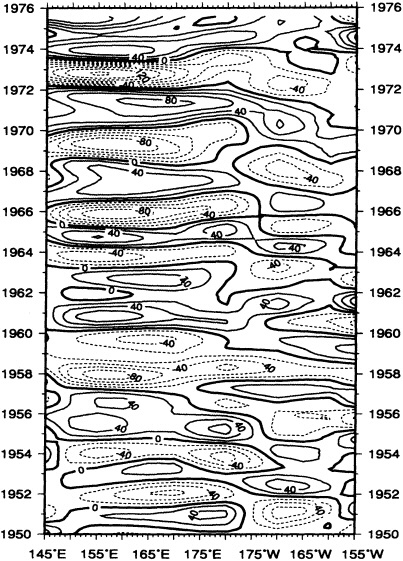
FIGURE 3
Time/longitude (Hovmöller) diagram of the total ENSO signal in sea-level height between approximately 145°E and 155°W. The diagram is based on spatial interpolation onto a regular grid of the SSA-filtered time series at eight stations slightly north of the equator (see text for details); latitude differences between stations are neglected. Contour interval is 20 mm (courtesy of Y. Sezginer-Unal).
Following the distinction made by Gene Rasmusson (Rasmusson et al., 1991) in the wind data, we also looked at the low-frequency mode (LFM) associated with ENSO (Figure 2, again in the color well). In that case, the amplitudes are even more tightly connected to the tropical Pacific and the west coast of the Americas. While a QBO-type oscillation does seem to be more global, this LFM is really concentrated in the tropical Pacific.
As for the spatial patterns, we took a group of eight stations just a little bit north of the equator in the western tropical Pacific and did a Hovmöller diagram (Figure 3). We wanted to look at the eastward-propagating signal in the quasi-biennial component of the zonal winds Dr. Rasmusson mentioned. We actually combined the two components, QBO and LFM. In this plot, which goes from 145°E to 155°W and includes data from 1950 to 1976, you can see that there is not so much a propagating as a standing signal, and actually there seems to be something of a nodal line about 175°W.
So I think that we are getting on with this business of trying to define the spatial modes of interannual and interdecadal variability, which obviously is more interesting than just looking at spectral peaks. And perhaps what we should be noticing is that the peaks are in the same places, not in different places, for various records.
Discussion
BRYAN: Do you suppose that the basic reason we don't see sea-level changes corresponding to the temperature changes in the climatic record is that the main signal, which reflects recovery from the Little Ice Age, is so large as to mask any other trends?
DOUGLAS: Well, the current rate of rise is close to 2 mm/yr, half of which is unaccounted for by glaciers and upper-layer warming. It's true that it may reflect a short-term readjustment, since we know archeologically that we haven't had a 4-m rise in the last 2000 years. But I think the only thing we can conclude from the tide-gauge record is that there hasn't been any acceleration in the last 100 or 150 years.
GHIL: Some of the high-latitude records suggest that the internal variability in sea level substantially exceeds the warming trend of about 20 mm in 10 years.
LEVITUS: The interannual sea-level changes at Bermuda are highly correlated with the steric changes from the Panulirus station. We've found large-scale, basically mechanical displacements of the whole pycnocline in the subtropical gyre—but no simple explanation for them.
RASMUSSON: One of the great advantages we have in studying the ENSO cycle is that we know where to index it to get good results. Some of the things you were showing, Bruce, suggested that you could pick out index stations too. I think it's very important in maximizing results, and also for setting priorities on which stations should be maintained.
MUNK: I'd like to point out that a lot can be learned from seasonal variations in sea level—a 1-year period—which seems not to have been done adequately. To a first order, the seasonal variation is steric; you get a significant agreement between sea level and volumetric changes. As far as I know, no one has attempted to account for the observed seasonal variation in terms of the seasonal variation in wind-stress curl, which I think would be worthwhile.
My other point is that tide-gauge data will not really be useful until it is corrected for the structural variability. It's unacceptable to have the geologic noise be about the same magnitude as the oceanic noise. The technology for getting accuracy of a few millimeters in the movement of the ground to which the tide gauge is attached is available. Also, it seems to me that you'd learn more from a few gauges from which the crustal movement could be removed than from many observation points subject to unknown geologic variability.
DOUGLAS: I agree completely. In fact, my original proposal called for a dozen or so super-stations, where we could do density and geodetic measurements, but unfortunately they were too expensive to get funded.
KARL: Could you elaborate a little on the acceleration you didn't find and how that relates to global warming?
DOUGLAS: Well, we have nearly 150 years of good records with reasonable distribution, and overall they don't show any global acceleration of sea-level rise. That says that the 25 percent increase in CO2 over the last 100 years has not caused anything that would accelerate sea-level rise—yet.
LEHMAN: I'd just like to point out that there is no consensus on the mass-balance status of the Antarctic ice sheet. Recent Greenland ice-sheet data seem to support Zwaly's controversial estimates, which suggest that it might actually have a positive mass balance. There are large uncertainties about the effect of ice volume on sea level; if it's offsetting a steric or thermally induced rise, it could be an important indicator that the ocean is absorbing greenhouse heat.
DOUGLAS: We really need a satellite-mounted laser to monitor the Arctic and Antarctic.
DESER: The large accelerations in sea level at Charleston and Bermuda between about 1920 and 1940 correspond to a time when there was warming along the Gulf Stream. I suspect that any differences between them might reflect changes in transport in the Gulf Stream.
GHIL: Ingemar Holmström has performed the data reduction you suggest, applying empirical orthogonal functions. He found very little independent information in the Baltic tide gauges; the first EOF contains some 90 percent of the variance.
I think we could sum all this up by saying that tide gauges may have relatively little to say about global warming, but they have a lot to say about air-sea interaction on interdecadal time scales.
Acoustic Thermometry of Ocean Climate1
WALTER H. MUNK2
A number of the workshop participants have alluded to the good spatial coherence of climate fluctuations, present and past, measured at separated sites. A system of climate observations should take into account the fact that variability on decadal and century time scales is generally associated with large spatial scales. In the ocean, this means gyre and basin scales of the order of say, 10 megameters (10,000 km).
I wish to discuss briefly a program of measuring climate-related fluctuations in ocean temperatures. The speed of sound is a good temperature indicator, increasing by 4 m/s per degree centigrade. Travel time between separated sites A and B yields a spatial average of temperature along the transmission path between A and B. The separation can be as great as 10 megameters, a distance well matched to climate scales. In most cases such a spatial average is preferable to traditional point measurements.
The ocean is a very good propagator of sound. It has exceptional acoustic properties because of the existence of the "sound-fixing and ranging" (SOFAR) channel, a classical wave guide, typically at a depth of 1000 m. The SOFAR channel owes its existence to a minimum in sound speed, with sound increasing upward from the SOFAR axis with increasing temperature, and increasing downward from the axis with increasing pressure. Sound is trapped in the wave guide, and the attenuation at the lossy top and bottom boundaries is largely avoided.
In January 1991 we carried out a feasibility test to determine whether 10-megameter ranges were achievable. We would like to be able to measure changes of 5 millidegrees Kelvin per year. This number derives from various model studies of greenhouse warming, from temperature changes inferred from a sea-level rise of 2 mm per year, and from a few direct observational time series. An increase of 5 millidegrees per year translates to a decrease in travel time by 0.2 s per year. To measure this we need a time precision of better than 0.05 s per year. This in turn demands that we use stable and coded acoustic signals from electrically driven (non-explosive) sources.
Our 1991 feasibility test was aimed at determining whether such electric sources were of sufficient intensity to be heard at 10-megameter ranges, and whether the codes could maintain sufficient fidelity to be read at such distances. Both questions have been affirmatively answered. In fact, usable signals were read at 17-megameter ranges, almost halfway around the globe.
We are now aiming at developing a global acoustic network that can resolve variations on a gyre and basin scale. The array will be designed to monitor ambient variability on decadal and century scales, as well as to detect a possible greenhouse-induced ocean warming.
Transient Tracers as a Tool to Study Variability of Ocean Circulation
PETER SCHLOSSER1,2 AND WILLIAM M. SMETHIE, JR.1
ABSTRACT
During the past decades, a variety of anthropogenic trace substances have been delivered to the ocean surface at relatively well-known rates. These transient tracers are used to study deep-water formation processes and rates, and to estimate mean residence times of waters found in the thermocline. Long-term observations of transient tracers indicate that they are useful parameters for studying ocean variability. On the basis of a review of the main elements of the tracer methodology and tracer time series from the Greenland/Norwegian seas and the Deep Western Boundary Current along the east coast of North America we discuss the potential of transient tracers as a tool for studying variability of ocean circulation.
INTRODUCTION
Prediction of the potential impact of greenhouse gases on our present climate requires understanding of the major elements of the climate system, including the ocean. Of particular concern is the understanding of the natural variability of the climate system, which has to be subtracted from any observed climatic trend before its significance can be evaluated.
There are numerous tools that can be used to study variability in the ocean, such as long-term observations of the classical parameters, temperature and salinity, or of currents. A more recently developed tool is the measurement of trace substances of natural or anthropogenic origin that carry time information. The time information can be derived from radioactive decay (radioactive clock) or from time-dependent delivery of the tracers to the surface waters from which they spread into the deep basins (dye tracers). In principle, both steady-state tracers and transient tracers can be used to detect variability in the ocean. A basic requirement for the application of the tracer method to detection of ocean variability is that multiple observations be made over a period of time of a certain tracer in a specific water mass or at a fixed location. Unfortunately, few such tracer time series exist, and the existing observations cover a rather short time span.
However, the available data clearly demonstrate the potential of tracers for studies of ocean variability (e.g., Rhein, 1991; Schlosser et al., 1991a). In this contribution we review the principles of the transient-tracer methodology and discuss its potential for studies of ocean variability on the basis of two selected examples.
TRANSIENT TRACERS
This section reviews the properties of the transient tracers that are currently most widely used in oceanographic studies. We do not attempt to provide a complete assessment of all potential transient tracers, but concentrate on those which in our opinion hold the greatest promise for future regional and global studies.
Tritium/3He
Tritium (3H) is produced naturally in the upper atmosphere by interaction of cosmic rays with oxygen and nitrogen. It is oxidized to HTO and takes part in the hydrological cycle. The production rate of 0.5 ± 0.3 atoms cm-2 sec-1 (Craig and Lal, 1961) leads to natural tritium concentrations in continental precipitation of about 5 TU (see, e.g., Roether, 1967; 1 TU or tritium unit means a tritium-to-hydrogen ratio of 10–18). Natural tritium concentrations of ocean surface waters have been estimated to be close to 0.2 TU (see, e.g., Dreisigacker and Roether, 1978). Such relatively low tritium concentrations can be well measured with state-of-the-art technology (see below). However, the natural tritium signal was masked more or less completely by delivery of bomb tritium to the atmosphere, mainly during the surface nuclear-weapons tests in the early 1960s. The bomb tritium levels exceeded the natural tritium concentrations in continental precipitation by about 2 to 3 orders of magnitude (Weiss et al., 1978). The tritium concentrations of Northern Hemisphere surface waters were raised from about 0.2 to about 17 TU (Dreisigacker and Roether, 1978).
Tritium decays to 3He with a half-life of 12.43 years (Unterweger et al., 1980). Tritiogenic 3He elevates the 3He/4He ratio of the waters in the ocean by up to roughly 50 percent (typical values are between 0 percent near the surface and about 10 to 20 percent in the lower thermocline). For much of the ocean, the tritiogenic 3He component can be separated from the other helium components found in ocean waters (mainly atmospheric and mantle helium; see, e.g., Roether, 1989, and Schlosser, 1992). In these cases an apparent tritium/ 3He age can be calculated. (For details, see the section on tracer ratios below.)
Tritium was traditionally measured radiometrically, using either scintillation counters or proportional counters. The precision and detection limits achieved by radiometrical measurement are about ±2.5 to ±5 percent and 0.05 to 0.08 TU, respectively (Östlund and Brescher, 1982; Weiss et al., 1976). These values have been improved significantly by mass spectrometric measurement of tritium using the 3He ingrowth method (see, e.g., Clarke et al., 1976; Bayer et al., 1989; Jenkins et al., 1991). State-of-the-art mass spectrometric systems achieve precision of ± 1 to ± 2 percent and detection limits below 0.005 TU.
3He is measured mass spectrometrically. Typical precision of the 3He/4He ratio measurement is about ± 0.2 percent, and precision of the 4He measurement is of the order of ±0.5 to ±1 percent (Bayer et al., 1989; Jenkins et al., 1991).
Halocarbons
During the past decade several halocarbons have come into use as tracers of oceanographic processes. These substances include CFC-11, CFC-12, CFC-113, and carbon tetrachloride. They all have strong anthropogenic sources and are chemically stable in the troposphere. However, they decompose in the stratosphere, and their decomposition products cause ozone destruction. They are also greenhouse gases, and thus a considerable effort has been made to determine and to monitor their atmospheric concentration as a function of time. The well-known atmospheric time histories of these substances allow a boundary condition for their input to the oceans to be accurately determined, which is a fundamental requirement for obtaining quantitative information about ocean processes.
CFC-11 (CCl3F) and CFC-12 (CCl2F2) are by far the most widely measured halocarbons in the ocean. CFC-11 has been employed extensively as a propellant in aerosol spray cans, and also in many manufacturing processes, particularly the expansion of plastic foams. CFC-12 is the primary coolant used in refrigerators, and is used in air conditioners as well. The manufacture of CFC-12 began in the mid-1930s and that of CFC-11 in the early 1940s; both substances came into wide use in the 1950s. The atmospheric lifetimes for CFC-11 and CFC-12 have been estimated to be 74 and 111 years, respectively (Cunnold et al., 1986).
CFC-11 and CFC-12 are measured by gas chromatography with an electron-capture detector. Maximum concentrations in high-latitude surface waters are greater than 6 pmol kg-1 for CFC-11 and 3 pmol kg-1 for CFC-12. Concentrations as low as 0.01 pmol kg-1 can be detected. Measurements can be made at sea at a rate of 60 to 70 samples per day. The precision of the measurement, as reported by several different laboratories, is the larger of 0.01 pmol kg-1 or ± 1 percent. An intercalibration cruise conducted in 1989 showed that this level of agreement was approached for CFC-11 for six different laboratories, but for CFC-12 the level of agreement was the larger of 0.02 pmol kg-1 or ±2.5 to ±3 percent (Wallace, 1992). The SIO 1986 calibration scale, which is widely used for oceanographic measurements, is estimated to be accurate to ± 1.3 percent for CFC-11 and ± 0.5 percent for CFC-12 (Bullister and Weiss, 1988).
CFC-113 (CCl2FCClF2) has been used during the last couple of decades as a cleaning solvent in industry, particularly in the electronics industry. Its atmospheric concentration has been increasing much more rapidly than that of
CFC-11 or CFC-12 during this time, and Khalil and Rasmussen (1986) have estimated a 13 percent annual rate of increase from measurements made at Point Barrow, Alaska from 1983 to 1985. Like those of CFC-11 and CFC-12, the atmospheric lifetime of CFC-113 is long; it has been estimated to be between 136 and 195 years (Golombek and Prinn, 1989). Its potential as a tracer in oceanography was demonstrated by Wisegarver and Gammon (1988) from measurements in the North Pacific subarctic gyre, but few measurements have been reported since then.
Like CFC-11 and CFC-12, CFC-113 is measured by electron-capture gas chromatography. It has proven to be much more difficult to measure than CFC-11 or CFC-12. One reason for this is severe contamination problems. Much of the equipment used for the measurement, such as pressure regulators and valves, is cleaned with CFC-113 when it is manufactured. This causes problems not only with the analysis but also with preparation of standards. Another major problem has been interference by naturally occurring halocarbons. These problems are now being overcome, but there are not sufficient data to determine the precision and accuracy to which CFC-113 can be measured. Theoretically, it should be possible to make the measurement to the same accuracy and precision as have been achieved for CFC-11 and CFC-12.
Carbon tetrachloride (CCl4) is another man-made halocarbon that has been produced in significant quantities since the early 1900s. Widely employed for dry cleaning and as an industrial solvent, it is currently used as feedstock in the manufacture of CFC-11 and CFC-12. The most recent estimate of its atmospheric lifetime is 40 years, and its current rate of increase in the atmosphere is 1.3 percent per year (Simmonds et al., 1988). The input of carbon tetrachloride to the ocean extends back in time 3 to 4 decades earlier than the CFC-11 and CFC-12 input, and thus it has penetrated the subsurface waters of the ocean farther than CFC-11 or CFC-12.
CCl4 can also be measured by electron-capture gas chromatography, and this procedure is routinely used for air samples. Procedures for routine analysis of seawater samples are currently under development (e.g., Krysell and Wallace, 1988; Wallace et al., 1992).
85Krypton
85Kr is a radioactive noble gas with a half-life of 10.76 years. It is formed when uranium and plutonium undergo fission. Although there is a small natural abundance, anthropogenic sources are over 6 orders of magnitude greater than natural sources (Rozanski, 1979). The major anthropogenic source is fission in nuclear reactors used for energy and plutonium production; there was also some production during the atmospheric nuclear-weapons testing in the 1950s and early 1960s. In reactors, most of the 85Kr is trapped in the fuel rods and released to the atmosphere when the fuel rods are reprocessed. This is done almost exclusively in the Northern Hemisphere, and accounts for the approximately 20 percent difference in atmospheric concentrations between the Northern and Southern Hemispheres.
85Kr is measured by counting the β-particles emitted during radioactive decay. Approximately 200 liters of seawater are required for each analysis, and samples must be counted for about one week. Thus, only a few hundred samples have been measured. The accuracy of the measurement is about ± 5 percent for near-surface water and ± 10 percent for deeper water with concentrations less than 25 percent of surface values (Smethie and Mathieu, 1986).
Bomb 14C
Natural 14C is produced mainly in the stratosphere by the 14N(n,p) 14C reaction. It enters the ocean as 14CO2 via gas exchange between the ocean and the atmosphere. Natural 14C concentrations in ocean surface waters range from about −50 to − 150 permil (in the Δ notation; for details of the notation, see Stuiver and Pollach, 1977). During the surface tests of nuclear weapons, mainly in the late 1950s and early 1960s, a significant amount of bomb 14C was added to the natural inventory, increasing the atmospheric 14C concentrations by roughly 90 percent. Observation of the invasion of bomb 14C into the ocean can be used to study ocean variability. The behavior of 14C differs from that of CFCs or 85Kr, because the exchange time of 14C with the atmosphere is modified by the buffering effect of carbonate and bicarbonate ions dissolved in seawater. Typical times for equilibration of a 100 m thick water layer are of the order of a decade for 14C, while they are only of the order of several weeks for CFCs or 85Kr. 14C also yields information on the average CO2 invasion rate into ocean surface water. Until recently, 14C was measured radiometrically using low-level proportional counters (e.g., by Schoch and Münnich, 1981). This technique allows very precise measurements (lσ error: ± 2 to ± 4 permil). However, it requires collection of about 200 liters of water per sample and CO2 extraction at sea, which limits the currently available number of 14C data. The relatively new AMS (accelerator mass spectrometry) technique requires less than 0.5 liters of water per sample. Routine procedures for CO2 extraction from the water and preparation of graphite targets have been developed (e.g., Schlosser et al., 1987; Kromer et al., 1987). The best precision currently reached for AMS measurements of oceanic water samples is about ± 5 to ± 10 permil (see, e.g., Kromer et al., 1987), but this precision is sufficient for studies of the penetration of bomb 14C into the ocean.
BOUNDARY CONDITIONS
Tritium/3He
Tritium is delivered to the ocean by water-vapor exchange, precipitation, and river runoff (see, e.g., Weiss
and Roether, 1980). Using a hydrological model and tritium data in precipitation observed at numerous stations of the WMO/IAEA network, Weiss and Roether estimated the delivery of tritium to the oceans as a function of time and space. Using a complex atmospheric circulation model, Koster et al. (1989) derived tritium fluxes to the ocean similar to those estimated by Weiss and Roether (1980). Dreisigacker and Roether (1978) converted the flux boundary condition given by Weiss and Roether (1980) into a concentration boundary condition for the North Atlantic (between 20 and 60°N). This "Dreisigacker/Roether function" (Figure 1) was used either directly or in modified form in many tracer studies, among them Sarmiento (1983), Thiele et al. (1986), Smethie et al. (1986), Thiele and Sarmiento (1990), Heinze et al. (1990), and Schlosser et al. (1991 a). Recently, Doney et al. (1992) reevaluated the IAEA tritium data using a factor analysis. They derived tritium concentrations in precipitation as a function of time and space with an estimated error of ± 3 to ± 10 percent. These data can be used to derive a relatively accurate flux boundary condition for tritium.
Tritiogenic 3He is exchanged between the atmosphere and the ocean on a time scale of the order of I week to 1 month. Since the atmospheric helium concentration (5.24 ppm; Glueckauf and Paneth, 1945) as well as the 3He/4He ratio (1.384 X 10⁻⁶; Clarke et al., 1976) are constant for practical purposes, the 3He boundary condition for ocean surface water in equilibrium with the atmosphere is well defined. However, in areas of deep convection or in ice-covered regions, significant 3He excesses above solubility equilibrium can be observed (see, e.g., Fuchs et al., 1987; Schlosser et al., 1990).
Halocarbons
The first accurate measurements of CFC-11 and CFC-12 in the atmosphere were made in the mid-1970s. Since
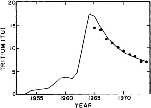
FIGURE 1
Tritium concentration in North Atlantic surface water as a function of time. (From Dreisigacker and Roether, 1978; reprinted with permission of Elsevier Science Publishers.)
1978, high-quality continuous measurements of both substances have been made at a number of different locations around the earth (see, e.g., Cunnold et al., 1986). McCarthy et al. (1977) have shown that the amount of CFC-11 and CFC-12 released to the atmosphere can be determined from the industrial production data, and atmospheric concentrations prior to the mid-1970s can be estimated from the amount of CFCs released. The cumulative amount of CFC-11 and CFC-12 in the atmosphere can be calculated as a function of time from this release data and the atmospheric lifetimes of CFC-11 and CFC-12. The atmospheric lifetimes have been estimated to be 57 to 105 years with a best estimate of 111 years for CFC-12 (Cunnold et al., 1986). The CFC inventory as a function of time can be calculated from
where I is the atmospheric CFC inventory in January of a given year, R is the amount of CFC released during a given year, ? is the reciprocal of the atmospheric lifetime of CFCs, and i denotes the year. Inventories are converted to concentrations by normalizing them to concentrations measured after the mid-1970s.
Smethie et al. (1988) used the procedure described above to estimate the CFC-11 and CFC-12 atmospheric concentrations as a function of time. The Chemical Manufacturers Association (1983) global release data were used; they are thought to be the most reliable up to 1976 because they contain Russian data for the 1968-to-1975 period. The normalization was done using 1976 data based on the SIO 1986 concentration scale. (Normalizations could have been done using data from later years, but the inventories are less accurate in later years because Russian data are not available after 1975.) The calculation was made using the extreme values for the atmospheric lifetimes, but this had only a small effect on estimated concentrations. The maximum difference in concentrations was 2.3 percent in 1950 decreasing to 0.3 percent in the mid-1970s for CFC-11, and 5 percent decreasing to 0.4 percent for CFC-12.
CFC-11 and CFC-12 concentrations for the Northern Hemisphere, based on the best estimate of the atmospheric lifetimes prior to 1976 and measurements after 1976, are shown in Figure 2. The production and use of CFCs occur mainly in the Northern Hemisphere, and concentrations of both CFC-11 and CFC-12 are 7 to 8 percent higher in the Northern Hemisphere than in the Southern Hemisphere (Cunnold et al., 1986), with a sharp decrease in concentration across the intertropical convergence zone. CFC-11 and CFC-12 are well mixed in both hemispheres, although concentrations above coastal waters can be a few percent higher than elsewhere in the atmosphere remote from land, particularly near the northeastern United States and Europe (Prather et al., 1987). The annual increase in CFC-11 and CFC-12 atmospheric concentrations is between 4 and 5 percent per
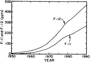
FIGURE 2
Atmospheric CFC-11 and CFC-12 concentration as a function of time for the Northern Hemisphere.
year today, but exceeded 20 percent per year in the past (Figure 3).
CFC-11 and CFC-12 enter the ocean from the atmosphere by gas exchange with an average equilibration time of the order of 1 month (Broecker and Peng, 1984). Therefore, most of the surface ocean is in equilibrium with the atmosphere, and the surface ocean concentration can be calculated from the atmospheric concentration and the CFC-11 and CFC-12 solubility. These solubilities are well known from laboratory measurements (Warner and Weiss, 1985); they are strongly dependent on temperature (Figure 4). In regions of the ocean where deep convection occurs, gas exchange may not be rapid enough to equilibrate the convecting waters, and low CFC concentrations have been observed in such regions. Bullister and Weiss (1983) observed CFC-11 and CFC-12 concentrations to be at 77 percent of satura-
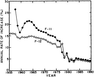
FIGURE 3
Annual rate of increase of the atmospheric CFC-11 and CFC-12 concentrations for the Northern Hemisphere.
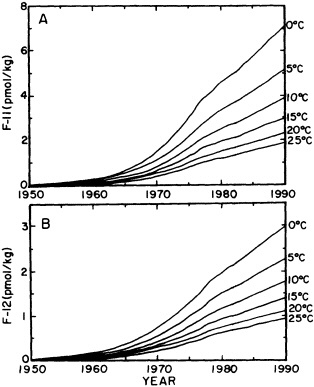
FIGURE 4
CFC-12 (a) and CFC-11 (b) concentrations of Northern Hemisphere surface water in equilibrium with the atmosphere for different temperatures.
tion in the Greenland Sea, and Wallace and Lazier (1988) observed recently formed Labrador Sea Water to be at 65 percent saturation. Since deep convection is an important process in the formation of many subsurface water masses, it is important to understand the extent to which these regions reach equilibrium with the atmosphere.
Atmospheric measurements of CFC-113 have been reported in the literature by two groups, the Oregon Graduate Center and the Climate Monitoring and Diagnostics Laboratory of NOAA. These results are reported on different calibration scales, and Golombek and Prinn (1989) have indicated that the concentrations reported on the Oregon Graduate Center scale may be 30 percent too low. The atmospheric concentration of CFC-113 can be estimated from industrial release data, as were those of CFC-11 and CFC-12. Such an estimate is presented in Figure 5. This curve was normalized to the concentration of CFC-113 at 35° over the western Pacific Ocean in 1987 measured by the NOAA Climate Monitoring and Diagnostics Laboratory (Thompson et al., 1990). Measurements made by the Oregon Graduate Center that have been increased by 30 percent are also plotted. The curve estimated from the industrial release data fits the observations well.
CFC-113 enters the ocean from the atmosphere by gas
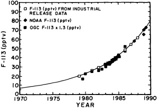
FIGURE 5
Northern Hemisphere atmospheric CFC-113 concentration as a function of time. The solid line is an exponential fit to the CFC-113 concentrations estimated from industrial-release data normalized to NOAA observations.
exchange, and as with CFC-11 and CFC-12, the surface ocean concentration should be in equilibrium with the atmosphere except in regions of active deep convection. Laboratory measurements of the solubility of CFC-113 are still in progress (Bu and Warner, 1995), but Wisegarver and Gammon (1988) estimated it from surface ocean observations where saturation levels of CFC-11 and CFC-12 were measured. It lies between the solubilities of CFC-11 and CFC-12.
The concentration of carbon tetrachloride in the atmosphere has been continuously measured since 1978, and its concentration prior to this time can be determined from industrial release data, as was done for CFC-11 and CFC-12. Its concentration in the Northern Hemisphere is 6 to 7 percent higher than in the Southern Hemisphere (Simmonds et al., 1988).
Carbon tetrachloride, CCl4, enters the ocean by gas exchange, as discussed above for other halocarbons. However, it is not as chemically stable in seawater as these other halocarbons. It slowly hydrolyzes, and Jeffers and Wolfe (1989) have estimated half-lives of 40 years at 25°C, 468 years at 10°C, and 2790 years at 0°C. This limits its usefulness in warm thermocline waters, though not in the cold deep water that comprises most of the ocean.
The atmospheric concentrations of the halocarbons discussed above are all well known as a function of time since the mid-1970s. Prior to this time, concentrations must be estimated from industrial production data. This is not so important for CFC-113, since it has been in use in significant quantities only since the early 1970s. For CFC-11 and CFC-12 the industrial production data are of high quality; they are thought to include 85 percent of global production. Thus, it is difficult to imagine that concentrations estimated from these data would be more than 5 to 10 percent in error. The production records for CCl4 are not as accurate as those for CFC-11 and CFC-12, and concentrations estimated from these data may have a larger error.
85Krypton
The 85Kr atmospheric concentration as a function of time is known from measurements taken at various locations over the earth since the 1950s (Rozanski, 1979). In the remote atmosphere there is a smooth increase with time, but there can be considerable variability in air masses that have been exposed to nuclear fuel reprocessing plants (Weiss et al., 1986). The concentrations in the Northern and Southern Hemispheres from a global atmospheric model fitted to observations (Rath, 1988) are shown in Figure 6. 85Kr enters the ocean by gas exchange with a roughly 30-day equilibration time, like the halocarbons discussed above.
Bomb 14C
The ?14C values of atmospheric CO2 as a function of time are fairly well known (Figure 7). The histories of ?14C in near-surface waters can be reconstructed from 14C measurements of growth-ring-dated corals (see Figure 8; examples appear in Druffel and Linick (1978) and Nozaki et al. (1978)). Using the known atmospheric 14C concentration, the CO2 exchange rate, and the surface water 14C concentration, we can estimate the expected 14C inventories for any station in the ocean (see, e.g., Broecker et al., 1985a). Comparison of calculated and observed inventories provides information on water mass transport. Observations made at different times yield information on variability of oceanic transport.
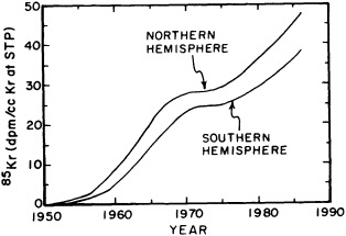
FIGURE 6
Atmospheric 85Kr concentration as a function of time from Rath's (1988) 2-D model fitted to observations.
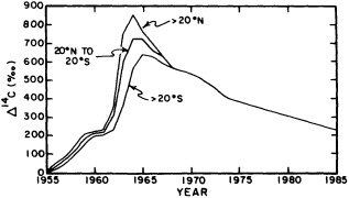
FIGURE 7
?14C in atmospheric CO2 as a function of time. (From Broecker et al., 1985a; reprinted with permission of the American Geophysical Union.)
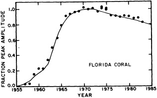
FIGURE 8
Shape of ?14C as a function of time for ocean surface water, based on 14C measurements of growth-ring-dated Floridian corals made by Druffel and Linick (1978). (From Broecker et al., 1985a; reprinted with permission of the American Geophysical Union.)
TRACER RATIOS
The presence of any of the substances discussed in this paper indicates that the water has interacted to some extent with the atmosphere within the past several decades. Since the measured concentration is a function of the initial concentration in the source water, which can be determined from the atmospheric time history, and the amount of mixing that has occurred since the water parcel left the source region, a model is needed to place further constraints on the age of the water.
Various tracers have different input functions, and thus tracer ratios vary in a unique way as a function of time. These ratios can be used as a water-mass age indicator. If the ratios are not altered by mixing, which is the case when a water parcel mixes with tracer-free water, they give a relatively accurate estimate of the time since the water parcel became isolated from the surface. Mixing of waters with different values of a specific tracer ratio can affect the age derived from this ratio in the same way as for absolute tracer concentrations. When a transient tracer first begins entering the ocean, the assumption of mixing with tracer-free water as a water parcel flows through the ocean is valid. However, with time the adjacent water begins to accumulate tracer by mixing, and this water, now tagged with tracer, mixes with newly formed subsurface water. Pickart et al. (1989) have shown for the Deep Western Boundary Current (DWBC) of the North Atlantic that this causes the CFC-11/CFC-12 ratio to be underestimated, and thus the age to be overestimated. This will be the case for any tracer/tracer ratio in which both tracers increase with time without radioactive decay. Thus, ages estimated by such a methodology are upper limits, and the inferred current speeds are lower limits.
Thiele and Sarmiento (1990), simulating the tracer ratio development in a Stommel-type gyre (Stommel, 1948), estimated the effect of mixing on ages derived from tritium/ 3He and CFC-11/CFC-12 ratios. They found that for a wide range of parameters their simulated tritium/ 3He ages were in very good agreement (about 10 percent) with a simulated true ventilation age. Deviations of simulated CFC-11/ CFC-12 ratio ages from their true ventilation age were significantly larger, particularly for lower ages, because the CFC-11 /CFC-12 ratio has been constant since the mid-1970s. Overall, the Thiele and Sarmiento simulations as well as the work done by Jenkins (1987) on tritium/3He show that certain tracer-ratio ages are very close to real ventilation ages in typical oceanographic settings.
Several tracer ratios that have potential for determining water-mass ages or mean residence times are discussed below. A summary of these ratios is presented in Table 1.
Tritium/3He Age
Parallel measurement of the radioactive mother/daughter nuclides tritium and 3He allows us to calculate the tritium/ 3He age of a water mass (see, e.g., Jenkins and Clarke, 1976). The tritium/3He age has to be considered an apparent age. It reflects the true age of a water parcel only in cases where eddy diffusion is negligible compared to advection. Its behavior is non-linear with respect to mixing (see, e.g., Jenkins, 1974; Schlosser, 1992). Addition of water free of tritium and tritiogenic 3He does not affect the tritium/3He age of this water mass. This means that if young water is mixed into an old water body with no tritium and tritiogenic 3He, the apparent tritium/3He age of the mixture is the same as that of the young water component. (For details of the tritium/3He dating method, see, e.g., Schlosser (1992).) However, simple model simulations show that the apparent tritium/3He age of a water parcel is close to the mean residence time of this water if the age is below about 10 to 13 years (Figure 9; Wallace et al., 1992).
TABLE 1 Summary of Tracer Ratios, Together with Approximate Age Ranges and Age Resolutions
|
Tracer Ratio |
Approximate Age Range |
Age Resolution |
|
Tritium/3He age |
mid-1960s to present |
± ˜ 3 months (present) to several years (1963) |
|
CFC-11/CFC-12 ratio |
mid-1950s to mid-1970s |
± 1 to ±2 years |
|
CFC-113/CFC-11 ratio |
1980 to present |
˜ ± 1 year |
|
CCl4/CFC-11 ratio |
mid-1950s to present |
˜ ± 1 to several years |
|
Tritium/85Kr ratio |
mid-1960s to present |
± 1 to ±4 years |
|
Tritium/CFC-11 ratio |
mid-1970s to present |
± 1 to ± 2 years |
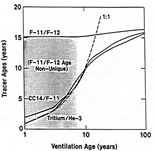
FIGURE 9
Apparent tracer ages obtained by a single mixed-box model versus ventilation age (mean residence time) of this box. The calculations were performed for the period between 1930 and 1987 (1987 values are plotted). The apparent tritium/3He ages (and CCl4/CFC-11 ages) are close to the mean residence time of the mixed box for mean residence times below about 10 to 13 years. (From Wallace et al., 1992; reprinted with permission of Pergamon Press.)
The apparent tritium/3He age of a water parcel is independent of its original tritium concentration. It therefore is a much better tool for estimation of mean residence times than absolute tritium concentrations alone. For waters with mean residence times below about a decade, the tritium/3He age is close to being a steady-state parameter. In addition, the time resolution of the tritium/3He age is very good (of the order of several months). The combination of these properties makes the tritium/3He age an ideal tool for studies of thermocline ventilation (see, e.g., Jenkins, 1987).
CFC-11/CFC-12 Ratio
From Figure 2 it can be seen that the atmospheric concentrations of CFC-11 and CFC-12 increased at different rates until the mid-1970s. CFC-11 increased at a faster rate, so the CFC-11 /CFC-12 ratio increased with time for different seawater temperatures, as shown in Figure 10. (The CFC-11/CFC-12 ratio in seawater increases at the same rate as that of the atmosphere, but the absolute values are different due to the different solubilities of CFC-11 and CFC-12 in seawater.) The CFC-11/CFC-12 ratio can be used to estimate ages of water parcels that left the surface between the mid-1950s and mid-1970s (see, e.g., Weiss et al., 1985; Smethie, 1993) with a resolution of ± 1 to ± 2 years. As discussed previously, these apparent ages are upper limits because of the effect of mixing. The ratio has been more or less constant since the mid-1970s, and for the past 15 years it is not useful for dating except to indicate that a water parcel was formed in the mid-1970s or later.
CFC-113/CFC-11 Ratio
CFC-113 has great potential as a tracer because of its rapid increase (13 percent per year) during the past 15 years. It ideally complements CFC-11 and CFC-12, whose ratio has been constant since the mid-1970s. A plot of the CFC-113/CFC-11 ratio for the atmosphere (Figure 11) indicates that the ratio is increasing at a rate of about 8 percent per year. The ratio in water will increase at the same rate, but
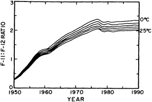
FIGURE 10
CFC-11/CFC-12 ratios as a function of time and temperature of Northern Hemisphere surface water.
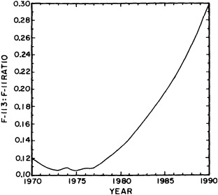
FIGURE 11
CFC-113/CFC-11 ratio as a function of time for the Northern Hemisphere.
will be different due to the differences in the solubilities of CFC-11 and CFC-113. If both CFC-11 and CFC-113 are measured to ± 2 percent, an age resolution of about 6 months can be achieved. However, the CFC-113 concentration in seawater is roughly an order of magnitude less than the CFC-11 concentration; for water that has been isolated from the surface for several years, the CFC-113 concentration will be less than 0.3 to 0.4 pmol kg-1. A more realistic measurement error for this concentration range is ±4 to ±5 percent, resulting in an age resolution at present of about 1 year.
CCl4/CFC-11 Ratio
Although carbon tetrachloride has been entering the ocean for a longer period of time than CFC-11, its rate of increase has generally been less than the rate of increase of CFC-11, and thus the CCl4/CFC-11 ratio has been continually decreasing with time (see Figure 12, from Krysell and Wallace, 1988). From 1950 to 1975, this ratio provides another estimate of water-mass age in addition to that provided by the CFC-11/CFC-12 ratio. Since 1975, the CFC-11 concentration has been increasing at 4 to 5 percent per year, and CCl4 at 1.3 percent per year. Therefore, the ratio is decreasing at about 3 percent per year, and if both CFC-11 and CCl4 are measured to ± 1 percent, an age resolution of ± 1 year can be achieved. An age resolution of ± 2 years is more realistic.
Tritium/85Krypton Ratio
Since the early 1960s tritium input to the ocean from the bomb spike has been continually decreasing, and 85Kr
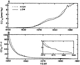
FIGURE 12
(a) Equilibrium surface water concentration of CCl4 in the Northern Hemisphere. (b) CCl4/CFC-11 ratio for Northern Hemisphere surface ocean water in equilibrium with the atmosphere. (From Krysell and Wallace, 1988; reprinted with permission of the American Association for the Advancement of Science.)
input has been continuously increasing. Therefore, the tritium/85Kr ratio decreases strongly with time. Both substances are radioactive, but decay at nearly the same rate (the half-life of tritium is 12.43 years, only slightly larger than 10.76 years for 85Kr). The small difference in decay rate causes the ratio to change by about 1 percent per year, but this change can be calculated and a correction applied. Smethie and Swift (1989) determined the time history of the tritium/85Kr ratio for Denmark Strait Overflow Water (DSOW) (Figure 13); from the measured ratio just downstream of Denmark Strait, they estimated that pure DSOW resided behind the Denmark Strait sill for no longer than a year. They also used the measured ratio in Gibbs Fracture Zone Water at the same location to estimate that about
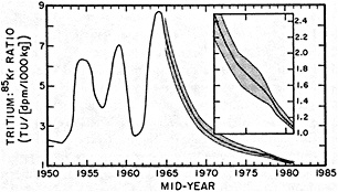
FIGURE 13
Tritium/85Kr ratio of Iceland Sea surface water as a function of time (corrected for radioactive decay). (From Smethie and Swift, 1989; reprinted with permission of the American Geophysical Union.)
7.5 years was required for it to be transported from its source region. The age resolution for the 3He/85Kr ratio is 1± to ±4 years.
CFC-11/Tritium Ratio
In the Southern Hemisphere, tritium/3He dating is severely limited, due to the low tritium concentration in surface waters and a relatively high mantle-3He component. In addition, the CFC-11/CFC-12 ratio is fairly insensitive for the time after about 1975. This situation limits the palette of available tracer ratios for dating of young waters in the Southern Hemisphere. However, recent measurements of tritium and CFC-11 in the Weddell Sea indicate that the CFC-11/tritium ratio might be a useful parameter for tracer-ratio dating in this region (Schlosser et al., 1991b). The ratio must be corrected for radioactive decay of tritium. The decay-corrected CFC-11/tritium ratio increases as a function of time (Figure 14) at a rate of roughly 10 percent per year, yielding a time resolution of about ± 1 to ± 2 years.
EVALUATION OF TRANSIENT TRACER DATA
Since concentrations of transient tracers are continually increasing in the ocean, a time series of a single tracer usually does not reveal ocean variability directly. To determine whether there is variability, a model must be applied to the data. Depending on the hydrographic situation, the models can range from simple box models to complex general circulation models. If the model parameterizes water-mass formation (including exchange with the atmo-
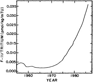
FIGURE 14
CFC-11/tritium ratio for Weddell Sea surface water (corrected for tritium decay).
sphere), circulation, and mixing in a reasonable way and can fit the time series with a set of constant (with respect to time) parameters, then little or no variability is suggested. If one or more of the parameters used in the model (for example, exchange rates between the individual water masses) must be changed as a function of time to fit the data, then there is variability. In special cases qualitative information can be derived from a single tracer time series. For example, if the concentration of a tracer with increasing surface concentrations increases in the deep water for a certain period of time and then suddenly stays at a constant level, there is a strong indication that the deep-water formation rate has changed.
Time series of tracer/tracer ratios might be used in special cases to determine whether there is variability without a model. If there is no variability in formation, circulation, or mixing (mixing has to be weak), water-mass ages estimated from the ratios should not change with time. Changes in the age would indicate variability in the formation rate of a specific water mass, its exchange rate with other water masses, or its transfer time from the formation region to the location of observation.
Straightforward application of tracer-ratio dating might work best on isopycnals in the thermocline (Thiele and Sarmiento, 1990) or in advectively dominated boundary currents (Smethie, 1993; see below).
EXAMPLES OF TRACER TIME SERIES
Atlantic Deep Western Boundary Current
CFC-11 and CFC-12 observations in the deep core of the DWBC in the Atlantic between 32° and 44°N were taken in 1983, 1986, and 1990 (Figure 15). Four sections across the DWBC were obtained in 1983, three sections in 1986, and five sections in 1990, with some overlap between the three surveys. In all of these sections there were two high-CFC-concentration cores adjacent to the western boundary: an upper core with a potential temperature of about 4.5°C at about 850 m depth, and a deep core with a potential temperature of about 2°C at about 3500 m depth (Figure 16). The upper core appears to be formed by wintertime convection in the southern Labrador Sea region (Pickart, 1992a), but is too warm to be classical Labrador Sea Water (Pickart, 1992a; Fine and Molinari, 1988). The lower core consists of the waters that flow over the Denmark Strait sill and the Scotland-Iceland Ridge (Smethie, 1993). The source waters for both cores interact extensively with the atmosphere and thus become tagged with high levels of CFCs. The high CFC concentrations within the cores indicate that the water in these cores formed more recently than adjacent deep water. This is also apparent in the CFC-11/CFC-12 ratios, which are higher in the cores than in the adjacent water (Figure 16).
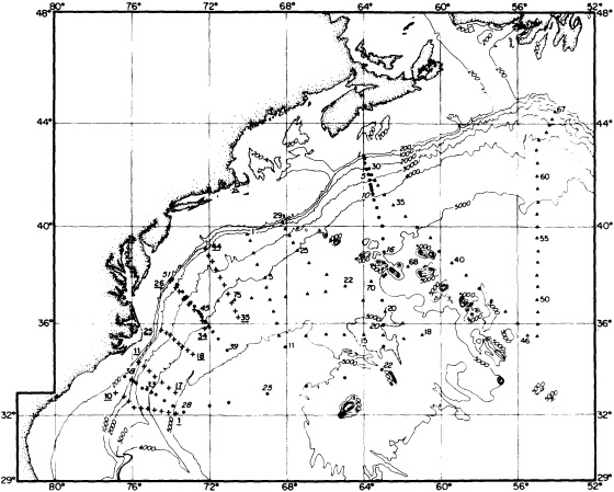
FIGURE 15
Station locations for the 1983, 1986, and 1990 surveys of the Deep Western Boundary Current.
These observations can be used in two ways to examine temporal variability in the DWBC: (1) Ages of the cores can be estimated from the CFC-11/CFC-12 ratio and compared for the different sections, as discussed in the previous chapter. (2) The CFC concentration can be used to identify the most recently formed component of the DWBC, as Pickart (1992b) has done using oxygen, and the temperature and salinity characteristics of this component can be compared at different locations and at different times at the same location along the western boundary current. This has been done for the deep CFC maximum for the 1983, 1986, and 1990 surveys.
For all three surveys the CFC-11 and CFC-12 concentrations in the deep core of the DWBC decrease in the downstream direction, and increase with time (Figure 17). These patterns are as expected, since the CFC-11 and CFC-12 concentrations have been continually increasing with time in the source waters. Ages of the deep core water estimated from the CFC-11/CFC-12 ratio increase in the downstream direction; this is also as expected, since younger water should be found closer to the source region. These ages increase in a linear fashion with distance from the source region, indicating that the apparent mean velocity of the current does not vary with distance from the source region (Figure 17). This apparent mean velocity is about 1.2 cm sec-1. It should be kept in mind that mixing causes the CFC-11/CFC-12 ratio age to be overestimated and the mean velocity of the current to be underestimated (Pickart et al., 1989). The important implication of these observations for temporal variability in the DWBC is that the estimated CFC-11/CFC-12 ratio ages from the three surveys lie along the same trend line when plotted versus distance from the source region (Figure 17). The estimated ages have an error of ± 1 to ± 1.5 years, which propagates to a ±5 to ± 10 percent error in apparent mean velocity, and there is roughly ± 10 percent variability in the calculated apparent mean velocity. This means that the age of the deep core between 32° and 44°N, as indicated by the CFC-11 /CFC-12 ratio, did not change by more than about 10 percent between 1983 and 1990, which implies that the combination of water-mass formation rate, transport, and mixing with adjacent water has been constant to within about ± 10 percent over this time period.
As mentioned above, the maximum CFC concentration
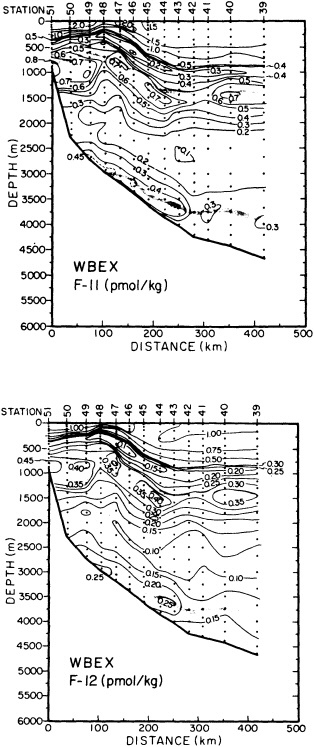

FIGURE 16
Vertical sections of CFC-11, CFC-12, and the CFC-11/CFC-12 ratio across the Deep Western Boundary Current at 36°N taken in 1986. (From Smethie, 1993; reprinted with permission of Pergamon Press Ltd.)
in the DWBC can be used to identify its most recently formed component. In this way the three surveys discussed above can be used to examine variability of temperature and salinity in the DWBC with time and distance along its flow path. Variability along the flow path also yields information on temporal variability because the DWBC can be thought of as a sequence of consecutive vintages of source water. A plot of temperature, salinity, and density versus distance from the source region shows some variability in space and time. The maximum differences between potential temperature, salinity, and density along the flow path are 0.17°C, 0.019 psu, and 0.026, respectively (Figure 18). The maximum differences between observations at the same location are 0.05°C, 0.007 psu, and 0.008. The combination of these findings and the observation that the water mass ages do not vary significantly with time suggests that small changes in the temperature/salinity characteristics of the source water can occur without changing the rate of formation, transport, and mixing of the deep core of the DWBC.
Some of the variability in the potential temperature and salinity of the DWBC core may be caused by not sampling the absolute CFC maximum due to vertical (100 to 150 m) and horizontal (20 to 30 km) sample spacing. Therefore, closer spacing should be used in future studies.
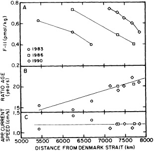
FIGURE 17
CFC-11 concentration (pmol kg-'), CFC-11/CFC-12 ratio age, and apparent mean current velocity calculated from the ratio age versus distance from Denmark Strait. Surveys were conducted in 1983, 1986, and 1990.
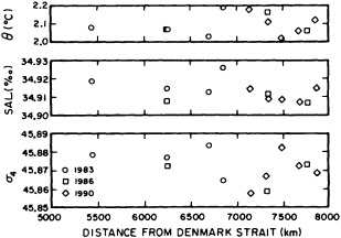
FIGURE 18
Potential temperature, salinity, and s4 versus distance from Denmark Strait for surveys conducted in 1983, 1986, and 1990.
European Polar Seas
Tracer data (mainly tritium and 3He, with some CFC-11/CFC-12 data) were collected between 1972 and 1988 at stations located in the Greenland and Norwegian seas (Figure 19). A small data set was also collected in the Eurasian Basin of the Arctic Ocean in 1984 and 1987 (Figure 19). The tracer concentrations in the deep waters (depth > 1500 m) of the Greenland and Norwegian seas are relatively homogeneous. Therefore, the concentrations in Greenland
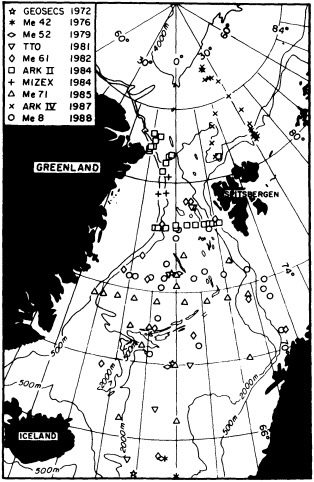
FIGURE 19
Tracer stations in the European polar seas occupied between 1972 and 1988. (From Schlosser et al., 1991; reprinted with permission of the American Association for the Advancement of Science.) Tracer data from these stations are used to construct the time series discussed in the text and displayed in Figure 20.
Sea Deep Water (GSDW) and Norwegian Sea Deep Water (NSDW) can be averaged for each survey. The time series of the averaged tritium and CFC-11 data of GSDW (Schlosser et al., 1991; Rhein, 1991; see Figure 20) show that the tritium concentration follows closely the curve expected from radioactive decay of tritium between 1980 and 1988, while the CFC-11 concentrations remained constant between 1982 and 1989. In addition, the tritium/3He age of GSDW increased more or less linearly between 1980 and 1988. These results suggest that almost no deep-water formation took place in the Greenland Sea in the period between 1980 and 1989.
A change in deep-water production was suggested as well by observations of temperature and salinity (GSP, 1990; Clarke et al., 1990). However, the salinity signals are small (of the order of 0.005 psu), and the T/S signal is definitely
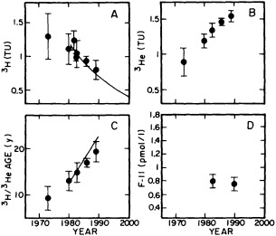
FIGURE 20
Temporal evolution of (A) the average tritium, (B) 3He, (C) tritium/3He age, and (D) CFC-11 values of Greenland Sea Deep Water (GSDW; depth > 1500 m). (From Schlosser et al., 1991; reprinted with permission of the American Association for the Advancement of Science.)
too small to be evaluated quantitatively. In contrast, the transient tracer signals are relatively large.
For quantitative evaluation of the transient tracer time series, a model is needed that simulates the basic exchange processes in the study area. In the case of the GSDW, we have to simulate the deep water formation and the coupling of the deep Greenland Sea to the Norwegian Sea and the Eurasian Basin of the Arctic Ocean. For this purpose, we modified a simple box model developed by Heinze et al. (1990) (Figure 21). The model allows deep-water formation
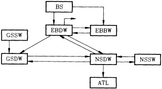
FIGURE 21
Box model used to simulate the GSDW tracer concentrations as a function of time. (NSDW: Norwegian Sea Deep Water; GSDW: Greenland Sea Deep Water; EBDW: Eurasian Basin Deep Water; EBBW: Eurasian Basin Bottom Water; BS: Barents Sea Water; GSSW: Greenland Sea Surface Water; NSSW: Norwegian Sea Surface Water; Atl: Overflow into Atlantic. (From Schlosser et al., 1991; reprinted with permission of the American Association for the Advancement of Science.)
in the main basins (Greenland Sea, Norwegian Sea, and Eurasian Basin). Exchange of deep water between the basins is implemented on the basis of hydrographic studies (Swift et al., 1983; Aagaard et al., 1985; Swift and Koltermann, 1988; Smethie et al., 1988). The model is then tuned to simulate a variety of steady-state and transient parameters in the deep waters (temperature, salinity, tritium, 3He, CFC-11, 85Kr, and 39Ar). The parameters used to tune the model are the deep water formation rates and the exchange rates of deep water between the individual basins.
The GSDW tracer time series can be reproduced by the model only if the formation rate of GSDW is variable (Figure 22; Schlosser et al., 1991a). The model requires a reduction of the GSDW formation rate by about 80 percent starting in 1980 (±2 years). With such an assumption the model fits the observations perfectly. Simulations of the tracer concentrations expected for the period between 1990 and 2000 for two scenarios with reduced deep-water formation rate (Figure 22, curve 2) and high deep-water formation rate (Figure 22, curve 3) show the sensitivity of the transient tracer approach for this particular region. The currently ongoing monitoring of tritium/3He and CFC-11/CFC-12 in the Greenland Sea should be a very good indicator of changes in the GSDW formation rate.
CONCLUSIONS
Existing data indicate that transient tracers are potentially valuable tools for studies of ocean variability on time scales
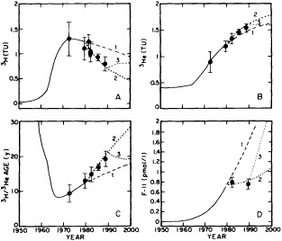
FIGURE 22
Comparison of observed and simulated tracer concentrations of GSDW for three scenarios: (1) constant renewal rate of GSDW; (2) GSDW renewal rate reduced by 80 percent starting in 1980; (3) GSDW formation rate reduced by 80 percent starting in 1980, followed by increase to full deep-water formation rate starting in 1990. A-D are as in Figure 20. (From Schlosser et al., 1991; reprinted with permission of the American Association for the Advancement of Science.)
of several years to several decades. Successful application requires careful selection of the best set of parameters for each case study. Typically, time series of a single tracer do not directly provide information on ocean variability. Therefore, models capable of parameterizing water-mass formation, including exchange of tracers with the atmosphere, ocean circulation, and mixing along flow paths, have to be applied to isolate the individual processes that affect the tracer concentration as a function of time. Tracer ratios might yield information on ocean variability more directly. Evaluation of the full potential of tracers as tools to study ocean variability clearly requires more and longer time series. Such time series could be obtained as part of the planned Global Ocean Observing System.
Long-term observations of transient tracers appear to be most useful for studies of deep- and bottom-water formation, as well as for investigation of the thermocline ventilation.
ACKNOWLEDGMENTS
We are grateful to Patty Catanzaro for drafting the figures. This work was supported by the National Science Foundation under contracts OCE 91-11404 (PS), OCE 8917801 (WMS), and OCE 90-19690 (WMS), and by the National Oceanic and Atmospheric Administration under contract NA16RC0512-01 (PS). LDEO Contribution No. 5295.
Commentary on the Paper of Schlosser and Smethie
JAMES H. SWIFT
Scripps Institution of Oceanography
The transient tracers, as Dr. Schlosser showed, provide real-world data on the time and space scales of ocean variability. In many cases, these are the only measurable information on these time scales, so I consider them extremely valuable for the conceptual understanding required for climate-type studies. (Like Dr. Schlosser, I am careful not to call them ''climate studies," because that is not what we are working with here.)
The observational network for providing the data for this type of study has many shortfalls, which is probably due to a shortage of resources. But I also have questions for Dr. Schlosser and the other workshop participants about whether we also need to fine-tune our notions of where we should carry out these studies.
My first question is whether there is a mismatch between the physical oceanography programs that provide water to people for the tracer studies, and the ideal data sets, you might say, required from the tracer studies. The freon, radiocarbon, and helium data are basically dependent on cruises that are, to a very great extent, planned and carried out by people in other fields. I wonder what sort of impact that has had on our ability to use the tracers.
Second, I notice that the many different groups carrying out tracer measurements are all under resource pressures. Is there a definite commitment from the investigators, in either the long or the short term, to getting the data from different sources together into a common set that we can use for global studies? We have a regional study in the western boundary undercurrent, a Greenland Sea study, and Antarctic studies. I should very much like to see their results being pooled into a single data base as the physical oceanography data are beginning to be.
Discussion
SCHLOSSER: The tracer groups are indeed working on establishing a common data set, but we still have some way to go before we can realize it. As for the tracer studies, I think we're getting closer to having the right platforms in the right places; in the process studies we're approaching an ideal tracer strategy. Of course, labor and resources continue to be limitations.
LEHMAN: You mentioned that recent observations suggest that ventilation has not recurred since the downturn in the 1980s. It was speculated that the GSA had quelled convection, but if ventilation hasn't recurred since the GSA's surface dissipation it would weaken any steric link between the two.
SCHLOSSER: We just don't know whether the GSA was involved, or how long it should take to restore the original mode. We're dealing mainly with the water below 1500 m,
but we also don't see a strong signal in the surface layer where we might expect it. We're just going to have to look at these complex dynamics more carefully.
LEHMAN: I noticed too that your data set indicates no diminution of the strength of the overflow or western boundary current. Before the shutoff of deep ventilation, the formation rate was about one-half a sverdrup, which means it would take 30 years to fill the basin. The overflow is controlled by the damming effect of the sills, so at 10 years after the shutoff we should now be one-third of the way through a cycle that should affect the overflow.
SCHLOSSER: But the overflow seems to be regulated to a very large extent by intermediate-depth convection, as Bob Dickson has pointed out. We may be seeing a phenomenon that is largely decoupled from the global circulation, but can give us insight into regional dynamics.
MYSAK: Isn't it in the Icelandic Sea rather than the Greenland Sea that the GSA caused the shutdown?
SWIFT: In my opinion, the overflows haven't changed; it's only the type of water that has changed. The current continues with whatever's at hand. The Arctic Ocean also outflows through the Denmark Strait, so you get high-salinity pulses from its intermediate waters as well.
RIND: Can you tell from the tracer data how much of the vertical mixing is associated with small-scale convection and how much with larger-scale overturning?
SCHLOSSER: We can only look at rates at present, not processes. We'd need a more elaborate model to do that.
TALLEY: Could you say something about the relative importance of sea-ice formation in open-ocean convection or in ventilating the Greenland, Norwegian, or Icelandic Seas?
SWIFT: In the conceptual model of Rudels and Quadfasel, which has the cyclic overturn, convection proceeds until the surface layer freezes. Then the brine released from further ice formation penetrates the warmer, saltier water underneath, bringing up heat, melting the ice, and starting another cycle. Deep-water formation appears to occur in the regions where the surface salinity and the heat and salt underneath are balanced so that this cycle can continue. The ice-formation process has to be parameterized as well.
WEAVER: I don't quite understand this concept of a western boundary current with constant magnitude but changing temperature and salinity. Wouldn't there be feedbacks that would force it to vary?
SWIFT: Well, that question is related to something I'd wanted to mention earlier. The models I've seen here seem to favor deep-ocean convection from the surface—the classic large-scale overturn. This focuses attention on "chimneys", which are relatively small-scale instabilities. But in the ocean the processes that prevail will be those that produce the densest water the fastest. For example, where there are continental shelves or ice shelves at high latitudes the local density can be greatly enhanced, partly because cooling is concentrated on a smaller total volume and dense products can accumulate, and you get the spreading Peter mentioned. This process may account for half the "deep convection" in the Arctic mediterranean seas. The point is that the environmental sensitivities of the continental-shelf processes are different from that of open ocean convection, which could affect the sensitivities used in modeling deepwater formation.
I guess that doesn't really answer your question, but I think we need to keep it in mind.
A Few Notes on a Recent Deep-Water Freshening1
JAMES H. SWIFT2
ABSTRACT
In 1981 much of the deep-water column of the northern North Atlantic was approximately 0.02 fresher than previous measurements had shown. These deep waters are closely tied to the sea surface in nearby water-mass formation regions, and the salinity change probably reflects the penetration into the ocean interior of the "great salinity anomaly" in the surface waters described by Dickson et al. (1988). The surface-layer freshening in the 1970s propagated into the deep water, because during winter the downward penetration of the cooled water depends on its density and not on its temperature or salinity alone. The net result of a freshening of the surface water is to produce colder, less saline water for a given density. This produced the changes seen in the 1981 data.
Until the 1980s there was virtually no modern-day evidence of any large-scale alteration in deep-ocean salinity. Oceanographers had not been accumulating high-precision deep salinity data long; nonetheless, the concept of a "steady-state ocean" was broadened by tradition to include the deep temperature and salinity fields. Small variations in deep-water salinity were observed in the western North Atlantic, particularly on the often-run Woods Hole-to-Bermuda section, but these were near the noise level and did not receive wide attention.
The GEOSECS (Geochemical Ocean Sections) program provided sparse, large-scale coverage of the North Atlantic in 1972. While the deep GEOSECS temperatures and salinities were similar to those from past expeditions, the GEOSECS data did show new features, notably a deep tongue of tritium-enriched water extending southward from the Denmark Strait. The presence of the deep tritium signal was a signal to oceanographers, showing that the bottom layers in the northwest Atlantic clearly responded on a time scale of 10 years or less to the injection of tritium into the atmosphere by thermonuclear testing.
Indeed, in general the best location to examine the deep ocean for evidence of recent property changes is the northern North Atlantic: It is close to the deep-water mass formation regions, and has been surveyed by expeditions 10 to 20 years apart.
The apparent sensitivity of the deep northwest Atlantic on 10-year (or less) time scales added immediate interest to the data gathered in 1981—nine years after GEOSECS—by the Transient Tracers in the Ocean North Atlantic Study (TTO/NAS). A total of 250 high-quality hydrographic-geochemical stations were occupied north of 17°N, a region covered by only 43 stations during GEOSECS. The TTO track provided some basin-scale sections, thus giving adequate coverage and facilitating comparison with other data from different years. Early reports in the summer and fall of 1981 from TTO/NAS indicated detectable changes in deep-ocean properties in the northern North Atlantic during the nine years following GEOSECS. Brewer et al. (1983) outlined the essentials of the new observations: a shift toward colder, fresher deep water in the northern North Atlantic and a larger freshening in the upper layers there.
The northern North Atlantic plays a significant role in the oceans' contribution to climate response, because it can be thought of as the primary deep ventilator of the world ocean. As Reid (1981) and others have shown, recently ventilated, or oxygenated, deep water spreads from the North Atlantic into the other oceans. Part of these high-oxygen waters derives from dense outflows to the North Atlantic from the Greenland, Iceland, and Norwegian seas, and part from processes within or over the deep northern basins of the Atlantic.
We can examine the northern sources by following a long section around the northern North Atlantic (Figure 1), following portions of the western boundary undercurrent. Note that the section and the undercurrent cut through a fracture zone in the mid-ocean ridge. This section passes near the overflows and the deep-water formation zone in the Labrador Sea. The sections in Figure 2 start in the Iceland-Scotland Overflow on the right, go through the
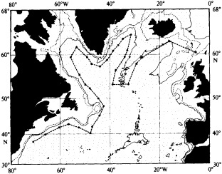
Charlie-Gibbs Fracture Zone and up to the northern Irminger and Labrador seas in the middle, then around the Grand Banks on the left. (There is a great deal of information in these sections—here I will discuss only a few of the features.) The middle section shows salinity versus potential density (s2, referred to 2000 db), not depth, and only for the denser portions of the water column. Because the Labrador Sea data are from winter cruises, when the density of the surface waters is higher, the upper line in that area follows the potential density at the surface. The bottom contour is bottom density, and it shows the contributions of dense water from the two main overflows.
There are differences in the salinities and final densities of the overflows. The Iceland-Scotland Overflow mixes with much warmer, saltier, and less dense water and forms a relatively high-salinity deep layer, underneath lower-salinity Labrador Sea Water. The Denmark Strait Overflow is a little fresher to begin with and mixes mostly with the layers immediately above, which are not so different. Thus the Denmark Strait Overflow retains its relatively low salinity and high density, and forms the bottom water in the northwest Atlantic.
The bottom section shows dissolved oxygen versus s2, along the same path. The three northern North Atlantic Deep Water sources are shown by the sources of relatively well-oxygenated water in the Labrador Sea, the Denmark Strait Overflow, and the Iceland-Scotland Overflow. The relatively well-oxygenated deep layer spreading south around the Grand Banks shows the propagation of the younger, overflow-derived deep waters southward via the western boundary undercurrent.
One of the results of this data analysis was an improved understanding that these deep-water components are closely tied to the winter sea surface and so are potentially sensitive to environmental changes. But during the 1957-1972 period emphasized in Figure 2, no such changes could be discerned in the deep temperature and salinity fields.
In the 1970s however, the surface layers of the northern North Atlantic freshened, by about 0. psu. European oceanographers call this "the great 1970s salinity anomaly" (cf., e.g., Dickson et al., 1988). The section in Figure 2 was well enough reoccupied in 1981 to permit comparison of the deep-water salinities before and after the surface-water freshening.
By 1981 deep-water salinities had changed throughout the northern North Atlantic. Figure 3 shows the salinity-versus-potential-density section from Figure 2, and the same section in 1981, contoured for the same ranges; it is clear that the 1981 salinities were lower than their earlier counterparts. The deep freshening was about 0.02 psu, and, since densities in each layer are about the same, we can see there was also an overall cooling, which in this case was about 0.15°C.
Figure 4 shows this deep temperature-salinity shift at
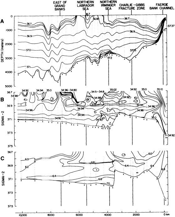
FIGURE 2
Vertical section from the Faeroe-Shetland Channel to the eastern U.S. continental margin of (A) s2 versus depth, (B) salinity (psu) versus s2, and (C) dissolved oxygen (ml/l) versus s2 (potential density anomaly referenced to 2000 decibars). Sections (A) and (B) are drawn from a composite of historical data (Chain, 1960, 1972; Crawford, 1960, 1965; Erika Dan, 1962; Atlantis, 1964; Hudson, 1967; Knorr, 1972, 1976) along the long, winding path shown in Figure 1. The only post-1972 data in (A) and (B) are from a single Knorr 1976 station in the Faeroe-Shetland Channel. Section (C) is drawn from April-October 1981 TTO/NAS data along a nearly identical path (see Swift, 1984a). Section (A) is contoured only for s2 > 36.7, and (B) and (C) show properties only where s2 = 36.7. The contour intervals are (A) 0.05 kg/m3, (B) 0.02 psu (for S = 34.8 psu), and (C) 0.2 ml/l. (From Swift, 1984b; reprinted with permission of Pergamon Press, Ltd.)
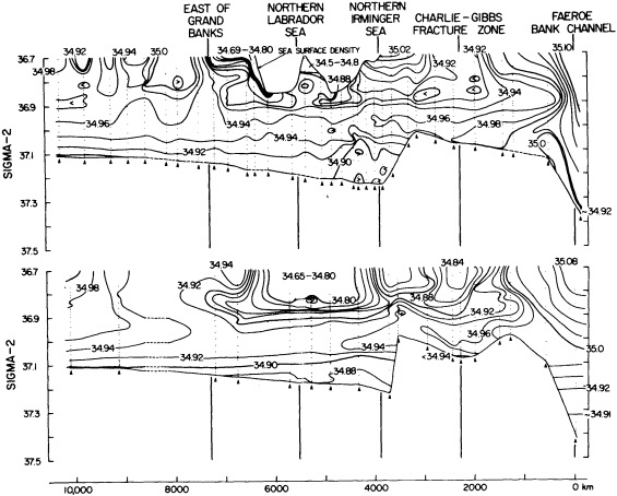
FIGURE 3
Sections of salinity (psu) versus s2 on a long, winding path from the Faeroe Bank Channel to the waters off the U.S. east coast (location shown in Figure 1). The upper section is from Figure 2, and the lower section is drawn from April-October 1981 TTO/ NAS data. The only post-1972 data in the upper section are from a single Knorr (1976) station in the Faeroe-Shetland Channel. (From Swift, 1984a; reprinted with permission of the American Geophysical Union.)
one location, in this case northeast of the Grand Banks. Four deep stations from 1960 to 1972 showed virtually the same potential temperature-salinity correlation, at least for deep waters colder than about 3°C. But the 1981 station at this location shows noticeably colder, fresher water-the changes are four standard deviations above the noise level. These changes occurred in virtually every deep-water layer in the North Atlantic north of 50°N.
The surface-layer freshening in the 1970s propagated into the deep water because in winter, in the water-mass formation areas, the downward penetration of the cooled water depends on its density and not on its temperature or salinity alone. The net result of a freshening of the surface water is to produce colder, less saline water for a given density. This produced the changes seen in the 1981 data.
The origin of the low salinities is an interesting puzzle. Figure 5 shows surface salinities before the salinity shift. The formation of dense waters in the Labrador and Greenland seas owes much to the salty water carried north at this and deeper levels. But much fresher water is plentiful along the boundaries. At first, I supposed that some shift in forcing in the 1970s allowed the fresh boundary waters to penetrate seaward into the deep gyres where the deep waters are formed. But we can see in Figure 5 that even in the pre-anomaly period the fresh-waters do not just flow south out of the northern North Atlantic. Instead their salinities are increased by vertical mixing and by lateral mixing, with much of the fresh-water incorporated into the gyres by the time they reach the Grand Banks. If during the 1970s the fresh-waters had simply spread away from the boundaries in the north and been mixed into the deeper layers there, then some areas of the far northeastern Atlantic farther "downstream" from the fresh source might be expected to increase in salinity, lacking the accustomed supply of fresh-water from the west. But since all the upper waters north of 50°N freshened, perhaps there was some net increase in fresh-water supply, or decrease in salty water supply, after 1972.
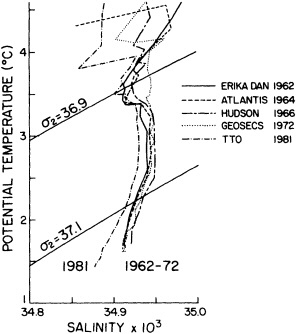
FIGURE 4
Potential temperature-salinity correlation below 4.5°C for four stations from 1962-1972 and from TTO/NAS (1981 data), all from a location northeast of the Grand Banks extending to about 3500 m. (From Swift, 1984b; reprinted with permission of Pergamon Press, Ltd.)
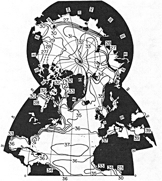
FIGURE 5
Salinity (psu) at the sea surface. (From Reid, 1979; reprinted with permission of Pergamon Press, Ltd.)
There may have been long-term changes in the atmospheric circulation coincident with this freshening. For an example of possible changes, consider Figure 6, which shows the difference between average wind-driven transport in the period 1973-1981 and that from 1955-1972. The changes are an average of about 30 percent of the mean at each grid point, and so may be significant. The negative values indicate a greater southward interior surface transport in recent years. Since the greatest negative values occur over the North Atlantic Drift, I wonder whether the high salts there might have been swept southward, partially shutting down the supply of salty water to the northeast Atlantic, and hence to the Labrador and Greenland, Iceland, and Norwegian seas. But Dickson et al. (1988) show that the freshening in the Faeroe-Shetland Channel took place late in an ordered sequence of events that began eight years earlier in the East Greenland Current, suggesting that it was a pulse-like increase in the volume of the fresh-water source that was at least in part responsible for the overall freshening.
We should remember that although these deep-water salinity changes (e.g., those in Figure 3) were the largest observed (at the time), they were still small in magnitude (only 20 parts per million). It may be that in the sinking zones only a small shift of the balance between precipitation and evaporation, or something similarly small, is at work here. In either event, this does illustrate the possible ties to large-scale atmospheric forcing of the deep thermohaline circulation, making the salinity shift, as we trace its propagation, one more tool with which to study the responsible processes.
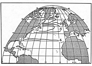
FIGURE 6
Change in integrated Sverdrup transport, average from 1973-1981 minus the average from 1955-1972. The transports were calculated from multi-year average sea level pressures on a 5° grid. Data from the Scripps Institution of Oceanography Climate Research Group. Owing to a minor (but non-recoverable) computational error, the values shown are not in sverdrups, but in nontraditional units. The average changes were 30 percent of the 1955-1972 base-period values.
The Salinity Decrease in the Labrador Sea over the Past Thirty Years
JOHN R.N. LAZIER1
ABSTRACT
Temperature and salinity data obtained in the Labrador Sea in 1966 and 1992 show that the average temperature and salinity of the 3500 db water column have decreased by 0.46°C and 0.059, respectively. The change in salinity is a maximum of approximately 0.09 at 2000 db in the Labrador Sea Water (LSW), an intermediate water mass that is renewed via deep convection in severe winters. The salinity difference diminishes to 0.05 in the Northwest Atlantic Bottom Water (NWABW) near the bottom and to 0.03 in the Northeast Atlantic Deep Water (NEADW), which lies between the LSW and the NWABW. An interrupted time series of salinity between 1962 and 1992 shows that anomalously low salinity occurred in the upper layer (0 to 250 db) between 1967 and 1972 and between 1978 and 1985. The salinity decrease in the LSW (1000 to 1500 db) occurs during two periods of rapid decline, 1972 to 1976 and 1988 to 1990, following the periods of low-salinity surface water. This suggests that deep convection is limited during the periods of low surface salinity and that, when convection resumes, the low-salinity surface water is mixed down to intermediate depths and serves to decrease the salinity of the intermediate LSW. Below the Labrador Sea Water the water column is strongly stratified, and the changes in salinity are due to changes in the properties of the incoming NWABW and NEADW rather than convection.
INTRODUCTION
The circulation in the Labrador Sea, first described by Smith et al. (1937), is dominated by a slow cyclonic gyre bordered by three strong currents (Figure 1). To the east is the West Greenland Current over the continental shelf and slope of southwest Greenland, to the west is the Labrador Current over the Labrador shelf and slope, and to the south is the North Atlantic Current flowing eastward at about 51°N. The West Greenland Current is a continuation of the East Greenland Current flowing south out of the Arctic along the eastern side of Greenland. It passes through the Denmark Strait and changes into the West Greenland Current after it rounds Cape Farewell at the southern tip of Greenland. On the inshore side of the West Greenland Current the water is cold (<0°C) and low in salinity (<34) (Grant, 1968). On the offshore side of this arctic water is a warm (4°C) saline (>34.95) band of water, which comes
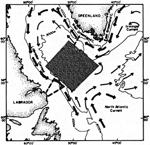
FIGURE 1
A map showing the general circulation of the Labrador Sea. The WOCE AR7/W line across the Labrador Sea and the CTD line used in the 1980s Labrador Current study are shown as dashed lines. The data used in this analysis were selected from the shaded region.
from the Irminger Current, a northern branch of the North Atlantic Current flowing north through the Irminger Sea toward Iceland. A significant portion of the West Greenland Current flows north into Baffin Bay, but most of the flow is thought to turn westward to the south of Davis Strait to become an offshore component of the Labrador Current.
The Labrador Current is a continuation of the Baffin Island Current flowing out of Baffin Bay through Davis Strait. It continues south over the continental shelves and slopes of Labrador and Newfoundland to the southern tip of the Grand Banks of Newfoundland. Like the West Greenland Current, the Labrador Current transports cold (<0°C) low-salinity water (<34) over the shelf and warm (>4°C) saline (>34.90) water over the slope.
The North Atlantic Current begins near the southern end of the Grand Banks of Newfoundland and brings subtropical water (T > 12°C, S > 35.5) north through the Newfoundland Basin into the southern Labrador Sea. Around 51°N, 44°W the current turns sharply east in what Worthington (1976) called the Northwest Corner. Although the subtropical water does not continue directly into the central Labrador Sea, the flow does appear to have some influence as far as 55°N, 50°W, where a weak northward flow turns east (Lazier and Wright, 1993).
The temperature field associated with the West Greenland and Labrador Currents is illustrated in the 1990 temperature section across the Labrador Sea shown in Figure 2. Over the continental shelves of both Greenland and Labrador is the cold (<0°C) arctic water. And over the continental slopes is the warmer Irminger water (>4°C) extending about 50 km out into the basin at 300 to 400 m depth.
In the central portion of the Labrador Sea (Figures 2 and 3) lies the nearly homogeneous Labrador Sea Water (LSW), which is renewed by deep convection in severe winters. From approximately 500 to 2000 db the temperature range is only 0.2°C, from 2.8 to 3.0°C, and the salinity range is only 0.02, from 34.82 to 34.84. The density as measured by the potential density anomaly (s?) referenced to 1500 db, s1.5, varies over the same pressure interval by 0.02 kg m-3, from 34.65 to 34.67 kg m-3. This is an average
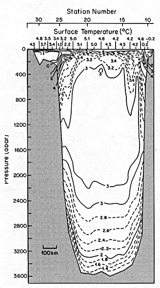
FIGURE 2
Potential temperature along the WOCE AR7/W line in July 1990.
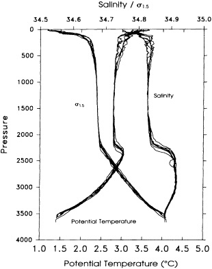
FIGURE 3
Profiles of potential temperature (?), salinity, and the potential density anomaly referenced to 1500 db (s1.5, in kg m-3) versus pressure (in db) at four stations in the middle of the AR7/W line in July 1990.
vertical density gradient of 1.33 × 10⁻⁵ kg m-4. (The renewal of the LSW is discussed by Lazier (1973), Clarke and Gascard (1983), Gascard and Clarke (1983), and Clarke and Coote (1988), while its circulation and distribution are considered by Talley and McCartney (1982).)
Below the LSW (Figure 3) the vertical density gradient is about an order of magnitude greater than in the LSW. The value of s1.5 varies from 34.67 kg m-3 at 2100 db to 34.90 kg m-3 at 3500 db, for an average vertical gradient of 1.6 × 10⁻⁴ kg m-4. Also, the variations of temperature and salinity below the LSW are much greater than those in it. In this deep stratified layer two water masses are usually identified: the Northeast Atlantic Deep Water (NEADW) and the Northwest Atlantic Bottom Water (NWABW). The NEADW is characterized by a salinity maximum S ˜ 34.92 between 2300 and 3000 db and potential temperatures of 2°C and 3°C. According to Swift (1984b), this water mass includes a component of the dense overflow from the Norwegian Sea through the Faeroe Bank Channel. This is modified by mixing with the water on the downstream side of the sill and flows into the western basin of the North Atlantic through the Charlie-Gibbs fracture zone. It then flows around both the Irminger and Labrador seas and is further modified through isopycnal mixing with the water flowing over the Denmark Strait.
The NWABW lies at the bottom of the water column and is identified by the decrease in salinity below the NEADW. Swift et al. (1980) conclude that this water is formed in winter at the sea surface north of Iceland. As it is the densest water in the region, it is not substantially modified through isopycnal mixing as it flows from the Denmark Strait to the Labrador Sea.
The purpose of this paper is to describe the decrease in salinity that has occurred throughout the water column over the past 30 years. The data base (Figure 4) begins with the observations from the Erika Dan cruise (Worthington and Wright, 1970). This is followed by the data collected at Ocean Weather Ship (OWS) Bravo throughout the years 1964 to 1973 inclusive and from stations on the 1966 cruise by C.S.S. Hudson (Lazier, 1973; Grant, 1968). The remaining data were obtained through the Transient Tracers of the Ocean (TTO) program's cruise to the Labrador Sea in 1981 and from various cruises made under the auspices of the Bedford Institute of Oceanography (BIO). The BIO efforts include 1976 and 1978 winter studies of the deep convection as well as the 1984 to 1988 data collected as part of a 10-year study of the Labrador Current (Lazier and Wright, 1993). The 1990 and 1992 data are from the World Ocean Circulation Experiment (WOCE) repeat hydrographic line AR7/W across the Labrador Sea collected by BIO. The positions of the conductivity-temperature depth (CTD) lines used for the Labrador Current study and the WOCE program are shown in Figure 1.
In the following section, data collected in June 1992 are compared with data obtained in 1966 in order to illustrate the gross changes in the water column. This comparison is followed by a presentation of time series of salinity from various layers. These demonstrate how the decrease in salinity in the LSW is determined through convection, which
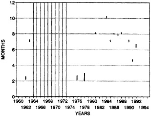
FIGURE 4
Periods of data collection in the central Labrador Sea.
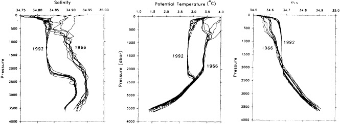
FIGURE 5
Temperature and salinity profiles obtained at six stations in the central Labrador Sea in March 1966 and at six stations in June 1992. Left, profiles of salinity; center, profiles of potential temperature; right, profiles of s1.5.
mixes low-salinity surface water down to intermediate depths, while the decreases in the NEADW and NWABW are controlled more by the salinity of the inflowing water. In a later section the changes in the temperature and density of the core of the LSW between 1962 and 1992 are presented.
1966 COMPARED TO 1992
Data obtained from six of the stations in the central Labrador Sea in March 1966 by C.S.S. Hudson are compared in Figures 5 and 6 with those obtained in June 1992 from six stations in roughly the same region. All these diagrams
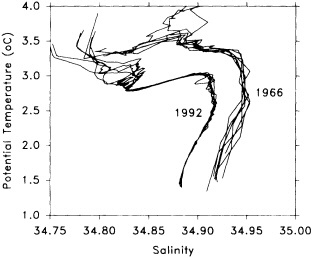
FIGURE 6
Potential temperature versus salinity for the stations plotted in Figure 5.
show that a remarkable change has occurred in the region over the 26-year interval. The average salinity over the whole water column has dropped from 34.92 to 34.861. This is equivalent to a loss of about 200 kg of salt per m2 of surface area or the addition of about 6 m of fresh-water per m2. The decrease in salinity is not constant throughout the water column but ranges from around 0.03 in the NEADW in the pressure interval between 2500 to 3000 db to around 0.04 in the NWABW at 3500 db. The greatest decrease is approximately 0.09 at 2000 db in the LSW.
The average temperature through the water column decreased by 0.46°C, from 3.144°C in 1966 to 2.686°C in 1992. This represents a total heat loss of 6.7 × 10⁶ kJ m-2 equivalent to a continuous loss over the 26 years of 8 W m-2. Most of the heat loss occurs in the LSW between 200 and 2300 db. In the NEADW and the NWABW the temperatures are only slightly less at a given pressure than they were in 1992.
The most significant difference between the deep temperature distributions of the two years is the erosion of the upper part of the NEADW by convection in the upper 2000 db. The profiles from 1966, for instance, suggest that the base of the LSW occurs around 2000 db at a temperature of 3.4°C, while in 1992 the base is around 2300 db at a temperature of 2.8°C. What were the upper layers of the NEADW in 1966 appear to have been incorporated into the LSW by 1992. Thus the water mass at a given density surface may change over time. This is discussed more fully later in the paper. The temperature maximum in the 1992 profiles at about 2400 db is another feature generated by the greater cooling in the LSW relative to the NEADW.
The profiles of sl.5 in Figure 5 indicate that the average density of the LSW is slightly greater in 1992 than it was in 1966, but that the vertical density gradient is less. The
strength of the gradient is thought to reflect the intensity of convection during the preceding winter. Thus the higher gradient in 1966 is evidence of a year when convection did not seem to be active (Lazier, 1973), while the lower gradient in 1992 is indicative of recent convection. The higher density in 1992 must reflect a higher-than-normal heat loss to the atmosphere in the years between 1966 and 1992, since the lowering of salinity over these years would tend to decrease the density. The heat loss has been sufficient to overcome the increased stratification due to the lower salinity, and cause convection to 2000 m or more.
The final comparison between 1966 and 1992 is shown by the temperature-versus-salinity curves in Figure 6. Here again the drop in salinity in the three main water masses is obvious, as is the fact that the difference in salinity is greater in the LSW than in the two deeper water masses.
In the following analysis, all the available data are used to construct time series of salinity in three layers in order to examine variations in time.
TIME SERIES OF SALINITY CHANGES
In Figure 7 the average salinities of three layers are plotted for all the years of available data. For each year,
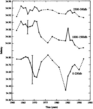
FIGURE 7
Average salinity in three layers between 1962 and 1992. The salinity scales for the 1000-to-1500 db and the 2500- to-3000 db curves are expanded five times relative to that for the 0-to-250 db curve. The vertical lines represent the maximum standard deviations associated with the data from OWS Bravo.
the data obtained within the shaded region in Figure 1 have been averaged together. In the years when data were collected at OWS Bravo, observations were collected in all months, so the averaged values approximate annual averages. The annual number of observations in the Bravo data varies a great deal, as does the number at each pressure level. In 1964, for example, 66 observations are recorded in the surface layers, but in 1969 (the peak year) there are 450 observations, and in 1973 there are 248. In the deep water the number of observations is more constant through the years. At 3000 db in 1966, 19 observations were obtained; in 1969 there are 11; and in 1973 there are 21. The standard deviations associated with the averages range from 0.08 to 0.2 in the near-surface layer, and from 0.01 to 0.02 in the deep layers.
In the years when Bravo data are not available, the values in Figure 7 have been obtained from one or two cruises. In these cases the averages are not annual averages, and do include any seasonal variation. Previous analyses of the Bravo data (Lazier, 1980) indicate that there are no significant seasonal signals in the intermediate or deep waters, so seasonal aliasing of the interannual signal will be a problem only in the 0-to-250 db curve. Since data were obtained at Bravo for 10 years, it should be possible to define the annual signal for the 0-to-250 db layer and remove it from the data collected in the non-Bravo years. This was not done, however, because the salinity in the upper layer at Bravo changed greatly over the 10 years of observation as a result of the arrival of the low-salinity pulse associated with the Great Salinity Anomaly. This large shift in the middle of the time series would distort the seasonal signal and make it unrepresentative of either the Bravo years or any of the other years.
The first curve plotted in Figure 7 represents the salinity in the surface layer from 0 to 250 db. The second curve is the average salinity from 1000 to 1500 db; it illustrates the changes in the LSW. The third curve shows the changes in the NADW from 2500 to 3000 db.
The surface layer is dominated by two large salinity decreases, in 1967 to 1971 and 1978 to 1985. The first of these is contained in the observations from OWS Bravo; it was discussed by Lazier (1980), who found that the lower salinity occurred during a period of mild winters. These higher winter temperatures, in combination with the increased stratification due to the higher vertical salinity gradient, limited the convection in winter to the upper few hundred meters. In 1972, however, a severe winter caused a renewal of convection to intermediate depths. The 19671972 low-salinity anomaly, which was also observed at other locations around the sub-polar gyre of the North Atlantic Ocean, became known as ''the Great Salinity Anomaly." Dickson et al. (1988) examined these observations, and were able to trace the path of the anomaly around the gyre;
they determined its speed of advance to be approximately 0.03 m s-1
The second period of low salinity (1978-1985) coincides with one observed by Myers et al. (1989) over the West Greenland shelf at Fylla Bank. In the middle of the Labrador Sea, however, there are only a few stations available, and the minimum is poorly sampled in both time and space. The fact that the salinity of the minimum appears to be less than that of the one in the 1967-1971 period is probably due to this poor sampling, which has allowed part of the seasonal cycle to be included.
In the intermediate layer, between 1000 and 1500 db, there is not a large change in salinity during the periods of low surface values, in 1967 to 1971 and 1978 to 1985. The most significant changes in this layer occur after the period of low salinity at the surface, when convection mixes the low-salinity water down to intermediate depths. For example, in 1972 and 1973, when the atmospheric conditions became more severe and convection returned, the low-salinity upper layer became mixed down into the intermediate layer. This is shown by the decrease in salinity from about 34.90 to 34.85 in the intermediate layer in 1972 and 1973, and the compensating increase in the upper layer from 34.53 to 34.84. A simple calculation of the salinity resulting from mixing the top 250 db at a salinity of 34.53 with the 250-to-1500 db clayer at 34.90 yields a 1500 db layer with a salinity of 34.84. This agrees with the observed value, within 0.01, and suggests that salt is conserved through the vertical mixing.
During the 1978-to-1985 salinity minimum there was again no significant drop in the intermediate layer's salinity. As in the earlier case, this is presumably because convection was limited to shallower depths. The salinity increase in 1985 seems unreasonably large, as no comparable increase occurred in either of the other layers. It is possible that the CTD salinity calibrations are incorrect at intermediate pressures but correct at higher pressures, but various checks have not yet found this to be so.
The second significant drop in the salinity of the LSW occurs between 1988 and 1990, when it went from 34.85 to less than 34.83. This decrease is similar to that of 1972 to 1976, in that it occurs after the minimum in the surface layer, and a restoration of convection in the late 1980s is the assumed cause. In contrast to the changes in 1972 to 1973, when the salinity increase in the upper layer occurred at the same time as the salinity decrease in the LSW layer, there appears to be a delay of about 3 years between the time when the salinity in the upper layer increased (1985-1987) and the 1988-1990 decrease in the LSW layer. There are two factors that may have caused this lag. The first is the fact that the salinity of the upper layer is badly aliased by the seasonal signal, so the actual decrease in salinity of the upper layer that is due to mixing with the intermediate layer is impossible to detect. The second factor is that mixing between the upper and intermediate layer is not the only way in which the salinity of the intermediate layer can change. Since that layer is fed partly by a component of the Denmark Strait overflow, its salinity will increase if the salinity of the Denmark Strait overflow increases as described below.
The third curve in Figure 7 shows the salinity changes in the 2500-to-3000 db layer that represents the NEADW. Since this water is in the more strongly stratified region of the water column, vertical mixing is small, and there should not be any connection between the salinity changes and events in the upper layer. For example, this layer does not exhibit decreases in salinity in 1972 to 1976 and 1988 to 1990 similar to those in the LSW. But there is definitely a decrease over the years, especially from the maximum of 34.94 in the mid-1960s to the present-day value of 34.915. The curves for the deep and intermediate layers also appear to be correlated during the periods when convection is not changing the LSW properties. This is especially true during the 1960s, when the two curves show increases and decreases of about the same magnitude at about the same time. A possible explanation of this correlation may be the influence of the water overflowing the Denmark Strait.
According to Mann (1969), the overflow water, which had a salinity of 34.93 in March 1967 and has a temperature that ranges between 0.5°C and -0.5°C. mixes with the warmer overlying water. This mixed water is not dense enough to reach the bottom, but it is of the same density range as the NEADW and the LSW. Thus, when these water masses flow south along the eastern slope of Greenland, the water on all the density surfaces is affected by either the dense overflow water at the bottom or the less dense mixed water that mixes with the LSW and the NEADW. When there is no convection in the central Labrador Sea, the changes in salinity in the intermediate and deep layers may therefore be regulated by the salinity of the overflow water and its mixtures. When convection is active, the salinity changes in the LSW are partly due to the convection and partly due to the changing properties of the mixed water formed south of the Denmark Strait.
TEMPERATURE AND DENSITY CHANGES IN THE LABRADOR SEA WATER
From the curves in Figures 3, 5, and 6, it is possible to define the properties of the LSW. For instance, the values of the temperature or salinity minima at intermediate depth can be recorded. But the water mass covers such a large pressure interval that the value of the temperature or salinity minimum and the pressure at which it occurs are often ambiguous. A more accurate way of defining the water properties is to plot temperature or salinity against density. Examples of temperature-versus-density curves are given
in Figure 8. These curves are from the 1966 and 1992 stations plotted in Figure 5. In addition to illustrating the warmest and coldest years, the curves present conditions when a definite minimum exists (1992) and when only an inflection point occurs (1966) in the LSW. The LSW can therefore be defined in 1992 by the temperature minimum of 2.8°C at a s1.5 of 34.675 kg m-3. In 1966 the water mass is defined by the inflection point in the curve at a temperature of 3.4°C at a s1.5 of 34.655 kg m-3.
By plotting all cruises in a similar way, a list of s1.5 versus minimum temperature values was obtained for the LSW. These are plotted against each other in Figure 9. As can be seen, from the beginning of the record in 1962, the temperature of the LSW increased from slightly greater than 3.2°C to 3.6°C in 1970 to 1971. At the same time the s1.5 decreased from about 34.65 to 34.63 kg m-3. These changes occurred during the period when deep convection was not taking place. The LSW was isolated from the upper layer, and the properties changed only through horizontal and vertical diffusion. In 1972 convection began again and caused the core temperature of the LSW to drop to 3.0°C at a density of s1.5 = 34.65 kg m-3.
Again in the 1980s, during the period of low surface salinities, convection was limited in depth, and the LSW became slightly warmer and less dense. This phase culminated in 1987, which is circled by a dashed line in the figure to indicate the indefinite nature of the determination. Convection appears to have begun again in 1988 and continued in 1990 and 1992.
The average s1.5, determined from the 18 values posted in Figure 9, is 34.650 kg m-3, with a standard deviation of 0.013 kg m-3. Thus all the values lie within one standard deviation of the mean, except for the years 1970, 1971, and
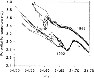
FIGURE 8
Potential temperature versus s1.5 curves for the same stations plotted in Figure 5.
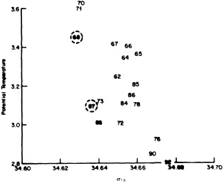
FIGURE 9
The value of potential temperature at the LSW minimum plotted against the s1.5 value where the minimum occurs. The numbers are the last two digits of the years of observations. When the values are indistinct, as in 1968 and 1987, the year is circled with a dashed line.
1968 on the low-density side and 1990 and 1992 on the high-density side. Without these five exceptional years, the density of the LSW is constant to within one standard deviation of the mean, while the temperature and salinity of the LSW have decreased by about 0.5°C and about 0.06. These figures support the suggestion of Clarke and Gascard (1983) that the density of the LSW remains constant over time because density changes due to temperature and salinity changes are equal and opposite.
The changes in density, although small through most years, are significant; in the 1960s a s1.5 of 34.675 kg m-3 represented the lower limit of the NADW, but in 1992 it was at the core of the LSW. It is clear that such a sigma surface cannot be used to monitor changes in the properties of either the LSW or the NEADW.
SUMMARY AND CONCLUSIONS
The changes in temperature and salinity at all depths in the Labrador Sea over the past 30 years have been demonstrated through the presentation of temperature and salinity data from the central portion of the sea. The changes between 1966 (during the most saline conditions) and 1992 (during the least saline) were presented in vertical profiles and ?-S curves. These showed that over the whole water column in 1992 there was approximately 200 kg m-2 less salt than in 1966 and about 6.7 × 10⁶ kJ m-2 less heat. The diagrams also demonstrated that the change in salinity was not the same at all depths, but ranged from around 0.03 in the NEADW to about 0.04 in the NWABW and about 0.09 in the LSW. The changes in salinity with time
were demonstrated using plots of average salinity in layers representing the near-surface conditions (0 to 250 db), the LSW (1000 to 1500 db), and the NEADW (2500 to 3000 db). The record in the upper layer was dominated by two periods of anomalously low salinity. The one in 1967 to 1971 is identified with the Great Salinity Anomaly, while the one in 1978 to 1985 is smaller and less well known. The anomalously fresh-water was subsequently mixed down to intermediate depths by convection, which caused the salinity of the LSW to decrease from 34.90 to 34.85 in 1972 to 1973 and from 34.85 to 34.83 in 1988 to 1992. The salinity decreases in the NEADW and NWABW were shown to differ from that in the intermediate LSW in that no influence of the deep convection was found. It was suggested that the conditions in the NEADW and NWABW are determined by isopycnal mixing between the mixed water created south of the Denmark Strait and the NEADW flowing into the Labrador Basin through the Charlie-Gibbs fracture zone in the mid-Atlantic Ridge.
The properties of the LSW were defined by the mid-depth temperature minimum or inflection in temperature versus s1.5 curves. A plot of the temperature at the temperature minimum versus the corresponding s1.5 demonstrated that the sl.5 of the LSW has varied from a low of 34.63 kg m-3 in 1970 to 1971 to a high of 34.675 kg m-3 in 1992. Because of this change in density over the years, it has been suggested that the properties of the water mass could not be accurately tracked through time by plotting temperature or salinity on a density surface.
Commentary on the Paper of Lazier
LYNNE D. TALLEY
Scripps Institution of Oceanography
I am greatly impressed by all the data that have been collected over the years. People need to understand how much individual effort goes into making sure that data continue to be collected, and Dr. Lazier is particularly to be commended for making sure that we have kept measurements going in the Labrador Sea. The Labrador Sea is one of the most important places in the world ocean for looking at the overall cycles of ventilation and overturn, and ultimately for understanding what determines SST.
Let me summarize some of the major points in Dr. Lazier's paper. The most important is that the Labrador Sea is a very significant site for deep convection. Labrador Sea Water affects a very big part of the water column in the northern North Atlantic; Figure 1 shows where it is found at mid-depth. Two water masses are in opposition—Labrador Sea Water, which is relatively fresh, and Mediterranean Water, which is salty. The salty Mediterranean Water is what makes the North Atlantic the saltiest of all oceans, and hence the likeliest for deep convection. The Labrador Sea Water provides an important fresher balance to the Mediterranean Water.
Why do we care about this? This may sound a little too simplistic, but on the very longest time scales and global spatial scales, what determines where deep water is formed, basin by basin, is which ocean is saltier and which ocean is fresher. Saltier surface water can be driven to higher density with cooling, so the salinity is what will determine the location of deep-water formation. The North Atlantic is currently relatively warm and salty—salty being the word to underline—and the deep water is formed there. In con-
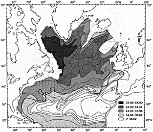
FIGURE 1
Salinity at the core of the Labrador Sea Water as defined by its potential vorticity minimum and at a potential density anomaly of 34.72 relative to 1500 dbar south of the heavy curve. The depth of the surface is approximately 1500 meters. (From Talley and McCartney, 1982; reprinted with the permission of the American Meteorological Society.)
trast, the North Pacific is a fresher ocean, and it receives its relatively salty deep water from the North Atlantic and Antarctic. Its surface layer is very strongly stratified or capped off in the subarctic gyre due to salinity.
The important consequence of this for modeling and for understanding the effect on the atmosphere is that the surface
layer can be colder in capped oceans than in overturning oceans. Simplistically, relatively fresh surface water can be cooled to freezing without overturning. So on very long time scales, the saltier ocean has the greater influence, and that probably comes down to the one that has the evaporative Mediterranean.
For deep-water formation in the Atlantic, the depth to which the overturn extends—and probably the surface temperature as a result—depends on the history of the overturn. Thus, if you want to understand the surface temperature or the temperature of the upper 500 meters, you have to be able to follow the history of the overturn.
I have one question I would like to pose to both Dr. Lazier and Dr. Dixon: Is there a possibility of capping off the North Atlantic completely in the current regime? You see the anomaly coming through. Could that anomaly be large enough or sustainable enough that North Atlantic conditions would be significantly changed?
It is clear to the oceanographic community that salinity is really important; it controls ventilation and overturning. Sea ice, evaporation, precipitation—all of which are things that we do not measure very well—are therefore important as well. If you have a global observing system without salinity measurements, you will be looking only at the result of what is going on; you will not be getting at the mechanism.
Obviously, salinity is not the whole answer; you need to know what the atmosphere is doing, and the forcing and all the interactions. But without salinity, you are stuck because the salinity controls overturn. The TOGA people are finding that to be true in the tropical Pacific. If you are thinking about where to monitor in a global observing system, you need to follow the history of the overturns, identify where overturns generally appear, and monitor them all the way through the depth of overturn. In the North Atlantic, you have to care about Labrador Sea Water down to where it shows up, and about overflow water—in short, the whole water column in the northern North Atlantic. In the North Pacific, I agree with Claes Rooth that you do not need to worry about deep water, but you might want to measure to 1500 meters. In each of the ocean basins some sort of argument can be made for where to monitor and, if you are looking at the water-mass structure, how deep to go.
We know very little about time scales, since we have an incredible dearth of time series. We are fortunate to have had the ocean weather ships in the past, as well as efforts such as John Lazier's to continue making measurements in the Labrador Sea. In the Pacific, there are equivalent data sets only in the California Current and around Japan.
Dr. Lazier's paper has demonstrated nicely the effect of two consecutive salinity anomalies. In both the convection was capped, with big property changes down below. A trend toward decreasing salinity and temperature can also be seen.
I had several questions in relation to the data shown. I was interested in the little blips of higher salinities during the capping. What is the source of the high salinity at depth during capping?
Second, I wondered whether there are enough data to tell whether there are 10- to 15-year cycles, or whether the overall decrease is part of a longer cycle. The earlier data are rather sporadic, so it may not be appropriate to use them to look at trends. And how are the two cycles related to the cycles that Syd Levitus showed?
And my last question is, how cold would you have had to make the water during those capping events in order to break through, and what kind of heat flux would it require?
Discussion
LAZIER: Capping the low-salinity water in the late 1970s was coincident with mild weather, and the same was true in the early 1980s. The succeeding severe weather resulted in mixing. Incidentally, two recent records indicate that the very-low-salinity Labrador Sea water is showing up in the Irminger Sea.
DICKSON: I think the real question was how you cap convection to the point that you interrupt North Atlantic Deep-Water production in some way. To start with, I'd say that we should be using the word "entrainment" rather than "convection" there. It's what's coming over the sill and doubling itself you worry about, not the deep-water convection where it got started.
Now if we compare the Denmark Strait overflow with the Mediterranean and gets up to a faster speed. It therefore entrains a large volume of unrelated, much less dense water—it multiplies itself by three—and comes down the slope with lots of turbulence. It ends up coming across at mid-depth, while the colder, more homogeneous Denmark Strait water outflow, the latter starts off denser, comes up a steeper slope, goes all the way to the bottom.
For the Greenland Sea, it would be easier to effect model changes by altering what is entrained rather than the density of the top 400 meters of the Icelandic Sea. And that could indeed change the production of deep water.
SWIFT: I wonder whether Walter Munk would comment on the scales of convection.
MUNK: Yes, I have a slide [see Munk, discussion after Lazier paper, in the color well] from a Greenland Sea experiment of
Peter Worcester and some others—their paper's in press—that might answer a question asked earlier. It's a tomographic representation of one full year, summer to summer, in the Greenland sea along four different sections. The data were taken every four hours, so it has unparalleled time resolution. You can see that you have very sudden—within about a day—penetration of cold water down to 1000 meters. Presumably this is a local effect, taking place at one spot along the 300-km transmission path. On the average, the upper water was lighter than the lower water when this occurred, so it was not a question of a massive overturning convection but of penetrating, chimney-like downward motions that formed some deep water.
LEHMAN: Obviously salt and entrainment are very important in determining some of the mechanisms and manifestations of the formation and composition of deep water. I think the question is how much water and heat content go north as a result of these processes we're monitoring. I'm beginning to agree with Wally Broecker that processes north of the Faeroe Ridge could almost be viewed as a single common-batch process. The key to some of the recent variability may lie in the Labrador Sea, where the water masses that are in the area of entrainment downstream are modified. We might also be seeing a real change in the flux of the formation of upper North Atlantic Deep Water. Climatologists really need to keep in mind that we may be able to explain the climate record in terms of how much heat these processes draw north with them.
BRYAN: We certainly need to remember that as we weigh the alternatives of instrumenting the whole Atlantic to look at the northward flow of the Norwegian current, or concentrating on the western boundary where we have currents moving southward.
LINDZEN: In the tropics the mean configuration of temperature and humidity is generally believed to be stable with respect to convection. Convection occurs due to local breakdowns in the mean, and cannot be anticipated on the basis of the mean itself. Therefore, when you look at mixtures and transports, the absence of gross instability is not necessarily germane to convection.
ROOTH: Also, in high latitudes there is a special factor that contributes to the significance of salinity anomalies: colder water is more compressible. When you cool water to the density at which convection can set in, a larger amount of potential energy is available, which enhances the intensity and depth of penetration of convection events. The correlation between the intensity of deep ventilation and the nature of the near-surface salinity anomalies is thus very important there.
The Local, Regional, and Global Significance of Exchanges through the Denmark Strait and Irminger Sea
ROBERT R. DICKSON1
ABSTRACT
The physical exchanges and transfers that have been observed to take place in the Irminger Sea and through the Denmark Strait are of local, regional, and global significance. The factors that control these processes, and their effects, are described according to these three distinct scales. The principal local effect is suggested to be a century-long modulation of the effectiveness of egg and larval drift between Iceland and Greenland, due to long-period wind-induced changes in the strength of the Irminger/West Greenland current system, with major implications for the cod fishery at both ends of the drift path. The exchanges of greatest regional importance are those associated with the approximately 14-year drift of the Great Salinity Anomaly around the Subpolar Gyre; here the key components are the anomalous production and export of ice and fresh-water from the high Arctic, the northerlies that brought it south in a swollen East Greenland Current, and the local processes that preserved the fresh-water layer north of Iceland prior to its export through the Denmark Strait. The transfers of global importance are the dense outflows of Arctic Intermediate Water and upper Polar Deep Water south through the deeper layers of the Denmark Strait, which contribute significantly to North Atlantic Deep Water production and thus drive the global thermohaline circulation. Some interactions between these three scales of processes are described, and some suggestions are made for improving the match between observation and simulation.
INTRODUCTION
This paper has two main aims: first, to describe the large-amplitude fluctuations that have characterized the physical environment of the Greenland-Iceland region at time scales of decades to those of a century or more; and second, to begin (but by no means complete) a description of their causes, controls, and effects over space scales that range from the local through the regional to the global and to provide some partial glimpses on how these scales may interrelate. With limited space available, this account will necessarily be brief; fortunately an extensive body of literature already exists to provide the details.
THE LOCAL SCALE: THE PHYSICAL MEDIATION OF BIOLOGICAL EXCHANGES BETWEEN ICELAND AND GREENLAND
During the twentieth century, the high latitudes of the Atlantic sector have undergone a considerable wave of warming and salinification that included the Iceland-Greenland region but was by no means confined to it. This change is illustrated in Figure 1 with reference to three of the longest series; the sea surface temperature anomalies for the West Greenland Banks from 1876-1974 (Figure 1a; Smed's data, in a succession of contributions to Annales Biologiques), the salinity of the upper North Atlantic Central Water layer passing northward through the Faeroe-Shetland Channel in
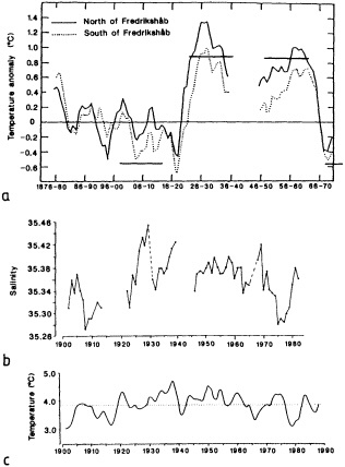
FIGURE 1
Increased warming and salinification during the current century. (a) Surface temperature anomalies for West Greenland, 1876-1974 (Smed's data, from Buch and Hansen, 1988; reprinted with permission). (b) the salinity of the North Atlantic Water in the Faroe-Shetland Channel, 1902-82 (from Dooley et al., 1984; reprinted with permission of the International Council for the Exploration of the Sea); and (c) 3-year running averages of yearly temperature along the Kola Section of the Barents Sea, 1900-90 (from Loeng, 1991; reprinted with permission of the Norsk Polarinstitutt), plotted to a common time base. The horizontal bars in Figure 1a refer to the warm and cold periods for which wind fields are compared in Figure 3.
1902-1982 (Figure 1b), and the 0-to-200 m mean temperature along the Kola meridian (33°30'E) in the Russian sector of the Barents Sea, 1900-1990 (Figure 1c). Many other temperature series—some from the open ocean (see Kushnir, 1994)—could have been adduced to make this point and, although long time series of salinity are less commonly available, we have sufficient glimpses of the salt record around the northern North Atlantic to suggest that the salinification was similarly pervasive, similarly protracted, and similarly extreme.
Thus as salinities rose to unprecedented values in the Faeroe-Shetland Channel in the late 1920s and 1930s (Tait, 1957; Dooley et al., 1984; see Figure 1b), extreme values were also being encountered further around the subpolar gyre in the U.S. Ice Patrol Standard Section running southwest from Cape Farewell. Some were so extreme as to provoke skepticism; as Harvey (1962) reminds us, "apart from 1933 when the salinity observations were thought to be in error, the highest salinity recorded by the US Coast Guard in any of their 22 observations along this section between 1928 and 1959 was a value of 35.07% observed in both August 1931 and July 1934."
In all cases, the period of peak warming and salinification occurred between the early 1930s and the late 1960s, and in a series of classic papers by Saemundsson (1934), Stephen (1938), Jensen (1939), Taning (1943, 1949), and Fridriksson (1949), we are left in no doubt that this wave of warming and salinification was accompanied by radical northward shifts in the distributional boundaries for a wide range of marine species.
In other words, both the circulation and the ecosystem of the subpolar gyre appear to have undergone a slow evolution over large space and time scales during the present century.
In socioeconomic terms, the impact of this widespread change reached a focus in the Iceland-Greenland sector, amplified through an apparent change in the effectiveness of egg and larval drift in the Irminger/West Greenland current system. The body of evidence is circumstantial but appears to be self-consistent. In Figure 2 below, Buch and Hansen (1988) indicate that the warming on the West Greenland Banks was accompanied by an explosive development of the West Greenland cod fishery (solid line), which rose from a negligible tonnage in the early 1920s to over 300,000 tons/year in the 1950s and 1960s and a maximum of more than 450,000 tons/year before abruptly declining once again between the late 1960s and the present as cooler conditions returned. Such "cod periods" have been documented in the past at West Greenland, in the 1820s and 1840s (Hansen, 1949), but this change represented a return of cod to West Greenland after an absence of at least 50 to 70 years (Buch and Hansen, 1988).
The hypothesis is that this change was both initiated and maintained by an increased exchange of cod larvae from
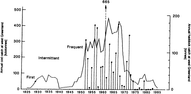
FIGURE 2
The catch of cod at West Greenland, 1925-85 (solid line; from Buch and Hansen, 1988; reprinted with permission) and the corresponding catch of haddock, 1952-83 (dots; data from Hovgård and Messtorff, 1987).
the spawning grounds off southwest Iceland during the warm decades, compared with the cold periods that preceded and succeeded them. Several items of evidence sustain this theory.
1. The Use of Haddock as a Tracer of Larval Exchange. Unlike cod, haddock do not spawn successfully at West Greenland, so if adult haddock are caught there they must have drifted there as larvae. (The closest known spawning site for haddock lies upstream near the cod spawning grounds off southwest Iceland.) When we compare the (small) international catch of haddock at West Greenland with the (large) international catch of cod (Figure 2), we find essentially similar trends of change in both species since 1952 when annual haddock catch statistics first became available (listed in Hovgård and Messtorff, 1987). There is even a qualitative similarity before that, with the first specimen of haddock reported from Greenland waters in 1929, infrequent occurrences in the 1930s, and frequent catches in 1945 (see Hovgård and Messtorff). Furthermore, in the years in which young fish surveys cover much of the drift path, the year (1984) with highest recorded abundance of 0-group cod off East Greenland (Vilhjalmsson and Magnusson, 1984) immediately preceded a very high abundance of 1-group cod at West Greenland (ICES, 1986). Thus while it is possible that the first cod colonizing the West Greenland Banks established a self-sustaining stock there, purely through the amelioration of the marine climate, the parallelism between cod and haddock catches along the western banks seems to argue that recruitment to the West Greenland cod stock was fed to a significant extent by a time-varying larval drift from Iceland.
2. The Analysis of Changes in the Windfield. Kushnir (1994 and personal communication) has analyzed the windfield changes that are associated with both short-term interannual variation of Atlantic SST and its long-term interdecadal variability. With Bjerknes (1964) he concludes that while the short-term variations in SST are governed by local forcing (windspeed and heat exchange), the interdecadal changes are governed by the non-local dynamics of the large-scale circulation. Figure 3a and b are truncated extracts from Kushnir's North Atlantic study, showing, for the area north of 40°N only, the change in windfield during winter (December to April) that occurred during the warming of the 1920s and the cooling of the late 1960s. The sense of the change has been made comparable by subtracting the 15-year cold-year average from the 15-year warm-year average in each case. Thus Figure 3a shows the change in the mean winter wind field from the cold period of 1900-1914 to the warm years of 1925-1939, while Figure 3b shows the equivalent change from the more recent cold episode of 1970-1984 to its antecedent warm period, 1950-1964. (These four periods are indicated by horizontal bars on Figure 1a.)
Since the Icelandic cod spawn off the Reykjanes Peninsula from March to May (Jonsson, 1982), these changes in the windfield overlap the season of egg liberation and early larval drift. And in each case the sense of the change from cold to warm periods has been one of increased easterly
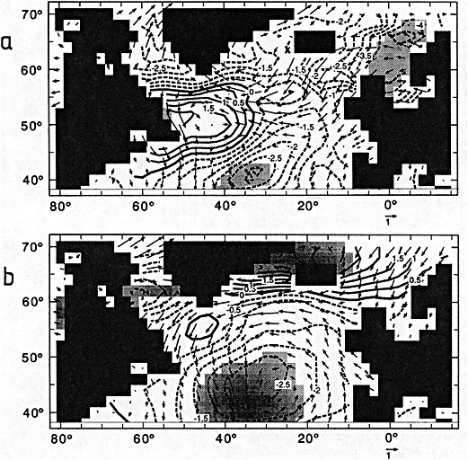
FIGURE 3
Change in winter-mean sea level pressure and winds associated with the change from cold to warm conditions in the northern North Atlantic. (a) Changes from 1900-14 (cold) to 1925-39 (warm); (b) changes from 1970-84 (cold) to the antecedent warm period, 1950-64. (Adapted from Kushnir, 1994; reprinted with permission of the American Meteorological Society.) These periods are indicated by horizontal bars in Figure 1a.
airflow overlying the westward-flowing Irminger current. While the simulation of the actual effect on the Irminger current awaits further refinement of the Comprehensive Ocean-Atmosphere Data Set (COADS) (Kushnir, pers. comm.), this result is at least qualitatively consistent with the hypothesis of increased larval exchange between Iceland and Greenland in the warm years of this century via the Irminger/West Greenland current system.
3. The Return Migration of Adults to Iceland. Economically, the effects of such changes are not confined to the effect on the cod catch at West Greenland. It is now becoming apparent that cod year classes that survive the drift to West Greenland as larvae may later return as adults to Iceland. These are not trivial events! Schopka (1991) shows that the return of the 1945 year class represented an unpredicted increment of over 700,000 tons of 8-year-old fish, worth more than £1 billion at today's prices (Figure 4).
The year-classes that Schopka lists as including adult immigrants to Iceland—1936, 1937, 1938, 1942, 1945, 1950, 1953, 1961, 1962, 1963, 1973, and 1984—are mostly those of the warm epoch, reinforcing the idea of more frequent emigration as larvae at that time, but even the infrequent occurrences of more recent years are of importance both economically and in terms of understanding which management measures were appropriate for the local Icelandic stock.
While certain components of the problem remain unresolved, the body of available evidence suggests that the local effect of a changing physical exchange between Iceland and
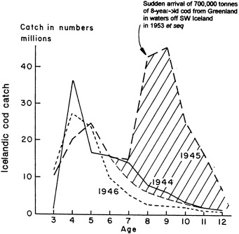
FIGURE 4
Catch-at-age curves for the 1944-46 year classes of cod at Iceland (from Schopka, 1991; reprinted with permission of the Northwest Atlantic Fisheries Organisation), but with the likely contribution of returning adults from Greenland shown hatched.
Greenland is an economic or socioeconomic one, acting to augment recruitment to the West Greenland cod population via larval drift from Iceland during years and decades when the wind field in winter and spring acted to strengthen the Irminger/West Greenland current system. A proportion of these fish may return as adults to Iceland.
Physically mediated exchanges of a similar type may also occur farther downstream along the same current system. As Templeman (1981) points out: ''Cod occasionally migrate from the Newfoundland area to West Greenland and vice versa (Templeman, 1974, 1979). Also in some years, especially 1957, there was considerable drift of cod larvae from Greenland toward the coasts of Baffin Island and Labrador (Hansen, 1958; Hermann et al., 1965)." (See also Templeman, 1965, and Danke, 1967.)
THE REGIONAL SCALE: THE "GREAT SALINITY ANOMALY" AND ITS LOCAL AND REMOTE CONTROLS
The widespread freshening of the upper 500 to 800 m of the northern North Atlantic, which has come to be known as the "Great Salinity Anomaly" (GSA), represents one of the most persistent and extreme variations in global ocean climate yet observed anywhere in this century. Dickson et al. (1988) describe it as largely an advective event, originating in the accumulation and preservation of an anomalously fresh near-surface layer in the seas north of Iceland in the middle to late 1960s, which was transferred through the Denmark Strait to the open North Atlantic in the late 1960s and was subsequently traceable around the subpolar gyre for over 14 years until its return to the Greenland Sea in 1981-1982. It is the first direct measure we have of the strength of the gyre circulation (about 3 cm s-1 on average). Figure 5 dates the passage of the GSA from its point of origin, through the Denmark Strait and around the Northern Gyre, while Figure 6 presents best-guess estimates of the salt deficit associated with the GSA at a series of points around this circuit.
The extreme nature of this event can be judged from the facts that as it passed south along the Labrador coast in 1971-1973 it represented a total salt deficit of some 72 × 109 tons; that in the eastern Atlantic, the observed freshening of about 0.1 psu to 500 m depth was the equivalent of adding an "extra" 1.4 m of fresh-water at the ocean surface (Pollard and Pu, 1985); that as it passed through the Faeroe-Shetland Channel in 1976 or so, the salinities in the North Atlantic and Arctic Intermediate Water masses were at their lowest since records began in 1902 (see Figure 1b); and that as it passed by northern Norway and west Spitsbergen in 1978-1979, the Norwegian Atlantic Current, by any conventional definition, ostensibly contained no Atlantic Water (i.e., water of salinity of 35 or more).
The chronology of this great event (Dickson et al., 1988) and its biological effects (e.g., Blindheim and Skjoldal,
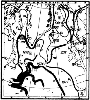
FIGURE 5
Transport scheme for the 0-1000 m layer of the northern North Atlantic, with dates of the GSA salinity minimum superimposed. (From Dickson et al., 1988; reprinted with permission of Pergamon Press.)
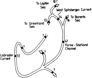
FIGURE 6
Estimates of salt deficit (× 109 tonnes) during the passage of the Great Salinity Anomaly around the northern North Atlantic. (From Dickson et al., 1988; reprinted with permission of Pergamon Press.)
1993) have already been thoroughly discussed and need not be repeated here. In the present context, the more relevant points for discussion are, first, to identify the near- and far-field controls that promoted and maintained such an extreme and protracted change and, second, to assess in the light of these controls whether we are dealing with a unique, occasional, or regular (even cyclical) event.
Various factors seem to have contributed to the amplitude and persistence of the GSA. These are conveniently discussed under four headings: (1) factors supporting the buildup of anomalously high pressure at Greenland during winters of the 1960s; (2) factors affecting the upstream supply of fresh-water; (3) local factors preserving the fresh-water layer north of Iceland, and (4) factors contributing to the persistence of the GSA downstream.
Factors Supporting the Build-up of High Pressure at Greenland During Winters of the 1960s
Dickson et al. (1988) ascribe the GSA primarily to the build-up of high pressure at Greenland from the mid-1950s to the late 1960s, in every season of the year but especially during winter (Figure 7). This change directed an abnormally strong northerly airflow over the Norwegian and Greenland seas, and as these northerlies increased to maximum strength in the late 1960s, the hydrographic character of the cold East Greenland and East Icelandic currents was altered. The East Greenland Current swelled in volume and became cooler and fresher as an increasing proportion of polar water was brought south from the Arctic Ocean to seas north of Iceland; the East Icelandic Current, which had been an ice-free Arctic Current during 1948-1963, became
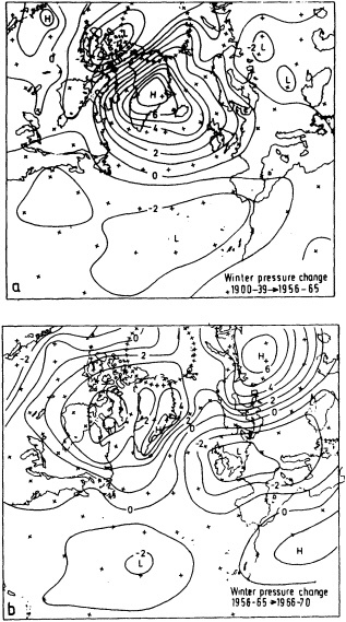
FIGURE 7
Mean change of winter sea level pressure (mb) between (a) 1900-39 and 1956-65 and (b) 1956-65 and 1966-70. (From Dickson et al., 1975; reprinted with permission of Macmillan Magazines Ltd.)
a polar current in 1965-1971, transporting and preserving drift ice.
Thus, it is the anomalous ridge at Greenland that is held responsible for bringing an increased supply of ice and fresh-water southward through the Greenland and Iceland Seas to the points of outflow into the North Atlantic, and thus for initiating the GSA (while, incidentally, terminating the warm epoch in Greenland waters, which formed the subject of the preceding section). After reaching a peak (5-year mean) anomaly of more than + 12 mb in winters 1966-1970, the ridge rapidly collapsed in the 1970s (recorded by Dickson et al., 1975), but by then the GSA was already a distant signal en route around the subpolar gyre.
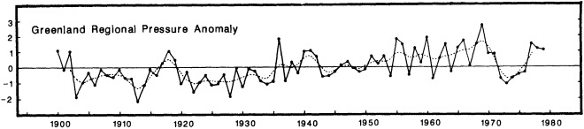
FIGURE 8
Normalized winter-mean pressure anomaly for the region 60-70°N, 30-65°W from 1900-1979. (From Rogers, 1984; reprinted with permission of the American Meteorological Society.)
The two most relevant questions in the present context are how unusual the Greenland Ridge of the 1960s was, and what factors might have contributed to its development. The first of these is addressed in Figures 8 and 9, which provide both a long-term and a hemispheric perspective. Figure 8 shows that the ridging that developed over Greenland in the late 1960s was unprecedented in a record of some 75 years' duration and, more remarkably, that it formed the end point of a steadily increasing trend in winter pressure there, which has been under way almost since the turn of the century. (The subsequent collapse of the Ridge in the 1970s is the event reported by Dickson et al. (1975).)
Even more remarkable is the spatial isolation of this change. In illustrating the difference in winter mean SLP between 1904-1925 and 1955-1971 (i.e., across the two endpoints of the above trend), Rogers shows (Figure 9 above) that the principal pressure change is confined to a restricted cell centered over Greenland, paired with a lesser
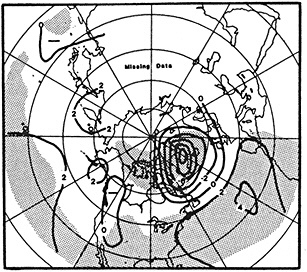
FIGURE 9
Difference in winter mean SLP between 1904-25 and 1955-71. Stippled areas are significant at the 95% level. (From Rogers, 1984; reprinted with permission of the American Meteorological Society.)
change of opposite sign near the Azores. Not surprisingly, then, the North Atlantic Oscillation (NAO = Azores - Iceland pressure difference) was at its century-long minimum also during the late 1960s (Figure 10).
Part of the reason for the shorter-term intensification of ridging at Greenland and decrease in the NAO between the mid-1940s and the late 1960s may be the processes that promote winter storm development in the zone of maximal land-sea temperature contrast along the U.S. eastern seaboard half a wavelength upstream. The reason for supposing such a connection lies in the notion that a steady strengthening of pressure at Greenland may more properly be regarded as a weakening of the statistical Iceland low. (A weakening Iceland low in twentieth-century Januaries has been noted by van Loon and Madden (1983).)
Dickson and Namias (1976) offer some support to this link by showing that a decadal change from a regime of warm winters (1948-1957) over the southeastern United States to a regime of cold winters there (1958-1969; Figure 11) was accompanied by a steepening of the thermal gradient at the coast, a sharp coastwise increase in the mean winter cyclone frequency (Figure 12) and a significant (approximately 350 nmi) southwestward retraction of the zone of maximum storm frequency as storms matured faster offshore. Thus, it remains a possibility that the record intensification of the Greenland High at this time (the 1960s) might in part be a reflection of a southwestward withdrawal of the statistical Iceland low.
The Upstream Supply of Ice and Fresh Water
The total salt deficit of the GSA as it passed the Labrador coast (72 × 109 tons—see Figure 6) is equivalent to a freshwater excess of 2000 km3. As Aagaard and Carmack (1989) point out, this quantity of fresh-water is too great to have its source in the Iceland Sea itself, but as the equivalent of about one-half of the annual fresh-water transport of the East Greenland Current where it enters the Greenland Sea from the Arctic Ocean, it can be accounted for by only a moderate perturbation of that outflow (e.g., a 2-year period of a fresh-water flux 25 percent above normal) and repre-
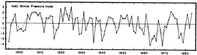
FIGURE 10
Winter index of the North Atlantic Oscillation (1895-1983) based on the mean normalized pressure difference between Ponta Delgada, Azores and Akureyri, Iceland. (From Rogers, 1984; reprinted with permission of the American Meteorological Society.)
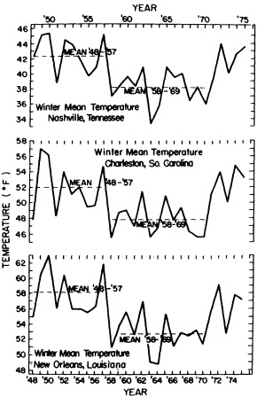
FIGURE 11
Winter mean air temperatures at Nashville, Charleston, and New Orleans, from 1947-48 to 1974-75. (From Dickson and Namias, 1976; reprinted with permission of the American Meteorological Society.)
sents an insignificant drain on the 100,000 km3 or so of the Arctic fresh-water reservoir. Thus, the fresh-water supply to the GSA is likely to have its origins upstream, in the processes of ice production and supply within the Arctic Ocean.
By comparing the timing of sea-ice variations in seven subregions that encircle the polar ocean over a 32-year period, Mysak and Manak (1989) were able to confirm a significant out-of-phase relationship between the ice-concentration anomalies of the Beaufort and Chukchi seas and the Greenland Sea. Later, Manak and Mysak (1989) and Mysak and Power (1991) extended and added detail to this sequence of relationships by showing, first, that fluctuations of the Mackenzie River discharge promote sea-ice anomalies of the same sign in the Beaufort and Chukchi seas about one year later and, second, that the export of large build-ups of sea-ice from the western Arctic via the Beaufort Gyre and the Transpolar Drift Stream would contribute to anomalies of ice extent and (from ice melt) freshwater supply in the Greenland Sea some 3-4 years after that.
Thus, annual runoff from the North American continent into the western Arctic precedes Koch's sea-ice severity index for the coast of Iceland by around 5 years (Figures 13a, b, c), and Mysak and Power (1991) conclude that the record freshets to the Arctic Basin in 1964-1966 (2 or more standard deviations from the mean; see Figure 13a) were significant precursors and suppliers of fresh-water to the GSA, as it developed in the Iceland and Greenland seas during the middle to late 1960s.
Local Preservation of the Fresh-water Layer in the Iceland Sea
The record extent of sea ice that developed in the Greenland and Iceland seas during the late 1960s (maximum in 1968) was partly the result of local as well as remote forcing, and was in fact a "telltale" of a local process that was fundamental to the preservation of an accumulating anomaly as large as the GSA: namely, by the mid-1960s the proportion of Polar Water in the East Greenland Current was so great that surface salinities north of Iceland decreased below the critical value of 34.7 (Figure 14). Below this value the surface layers will not reach a sufficiently high density,
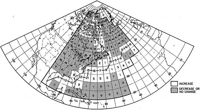
FIGURE 12
Change in the total number of cyclones between the "warm SE" and "cold SE" groups of winter months in the southeastern USA. (From Dickson and Namias, 1976; reprinted with permission of the American Meteorological Society.)
even at the freezing point, to mix with the underlying, more saline water (Figure 15); instead, ice will tend to form (Malmberg, 1969). Thus, not only was more fresh-water transported south toward Iceland during the 1960s (from whatever source) under the stress of an anomalous northerly airflow, but in the years of peak polar influence (1965-1971), the extremely cool, fresh character of the upper 200-300 m was preserved since it was not mixed out by convective overturn (Dickson et al., 1988).
Downstream Preservation of the Fresh-water Layer
Once the GSA has passed through the Denmark Strait and is undergoing its long circuit of the subpolar gyre, we are forced to be even more conjectural about the forces that might have maintained its integrity. One suggestion that is perhaps better based than most comes from Clarke (1984); it posits an interaction between the GSA and local environmental conditions as it passed south along the Labrador coast (see Figure 9 of Dickson et al., 1988). From the late 1960s until 1971-1972, and possibly for unconnected reasons, there was progressively less deep winter convection at OWS Bravo in the central Labrador Sea (Lazier, 1980). As a result, said Lazier, the surface layer at Bravo freshened and the offshore salinity gradient weakened, so that the offshore fresh-water flux by eddy-diffusive processes would have weakened also. For this reason, Clarke suggests that the GSA fresh-water signal would have been maintained rather than mixed offshore during its long circuit of the Labrador shelf and slope. Although convection at Bravo and the offshore salinity gradient were rapidly restored following the severe winter of 1972, the GSA signal had largely passed.
Periodicity
Our present patchy understanding of the GSA event suggests that the Arctic Ocean provided the fresh-water, the northerlies of the Greenland High brought it south, and conditions both north of Iceland and downstream prevented it from being mixed out (vertically and laterally). However, we have only an inconclusive answer to its likely periodicity. If the strength of the winter high-pressure cell at Greenland in the 1960s was a critical factor, as Dickson et al. (1988) claim, then that circumstance was a secular event—the product of a slow evolution over most of this century. If the maxima in Koch's sea-ice index indicate the same process of accumulation of fresh-water and suppression of convection north of Iceland as we describe in Figure 15, then there may be grounds for belief that an earlier, if lesser, salinity minimum in 1910-1914 (see, for example, Figure 1b) reflected a previous iteration of the GSA set of processes (Dickson et al., 1984). However, numerous authors have pointed to the scope for multiannual or decadal periodicity
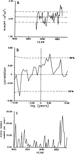
FIGURE 13
(a) Annual runoff from the North American continent into the Arctic Basin, 1930-67, with mean (solid line) and ± 1 standard deviation (dashed line) indicated; (b) lagged cross-correlation between runoff (above) and Koch Index of ice severity (below) at the Icelandic coast, 1915-75; (c) the Koch sea-ice severity index for Iceland. (All from Mysak and Power, 1991; reprinted with permission of the Canadian Meteorological and Oceanographic Society.)
that is inherent in such processes. The approximately 14-year circulation period of the subpolar gyre is plainly one such control, but the decadal regimes in southeastern U.S. air temperature shown in Figure 11, the 6.7-year spectral maximum in the North Atlantic oscillation index (Rogers,
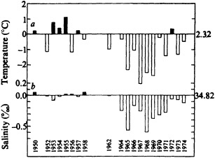
FIGURE 14
Anomalies of (a) temperature and (b) salinity in June at 25 m depth in a study area between Iceland and Jan Mayen (67- 69°N, 11-15°W). The long-term means, 1950-58, are also shown. (From Malmberg, 1973; reprinted with permission.)
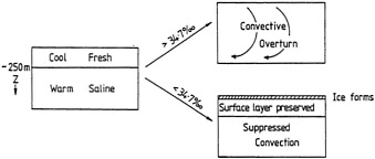
FIGURE 15
Schematic diagram illustrating the suppression of convection north of Iceland as upper-ocean salinities decrease below 34.7. (From Dickson et al., 1988; reprinted with permission of Pergamon Press.)
1984), the multi-year advective time lag of ice drift from the Beaufort Sea to Greenland and Labrador (Mysak and Power, 1991; Mysak and Manak, 1989) plainly have the potential to lend a degree of periodicity to the process. Conceptual models for these periodic anomalies—some of great complexity (see Figure 3 of Mysak and Power, 1991)—have been proposed (see also Darby and Mysak, 1993; Ikeda, 1990). Under this rationale the Great Salinity Anomaly was merely a more obvious, high-amplitude iteration of a regular event.
THE GLOBAL SCALE: PRODUCTION OF NORTH ATLANTIC DEEP WATER AND THE THERMOHALINE CIRCULATION
To demonstrate a global role for Denmark Strait exchanges, there can be few more eloquent illustrations than Figure 16 (from Charles and Fairbanks, 1992), in which the d13C history in benthic forams from the sea-floor sedi-
ments of the Southern Ocean is used to indicate the changing content of the North Atlantic Deep Water (NADW) in the abyssal circulation over the past 6,000 to 18,000 years. Since Circumpolar Deep Water consists of both NADW with a high d13C content and Indo-Pacific Deep Water with low d13C, the increase in d13C content at the end of the Ice Age is thought to reflect the rapid resumption of full NADW production at that time.
Whether or not we believe that NADW production was stopped or merely much reduced during the last glaciation, it is plain that the glacial-interglacial signal was reflected in the amount of NADW in circulation. Since the dense overflows across the Greenland-Scotland Ridge (plus consequent entrainment) constitute the largest two of the four main sources of NADW (see Figure 17, taken from Swift
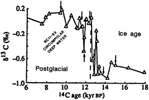
Figure 16
d13C record of benthic forams in Southern Ocean core, indicating the changing production of North Atlantic Deep Water, 6,000-18,000 BP. (From Charles and Fairbanks, 1992; reprinted with permission of Pergamon Press.)
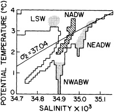
Figure 17
Potential temperature vs. salinity diagram for North Atlantic deep waters colder than 4°C, with the characteristics of NADW shown by hatching. (From Swift, 1984b; reprinted with permission of Pergamon Press.)
(1984b)), it is equally plain that a time-varying exchange between the sub-Arctic seas and the deep open Atlantic has had a global importance in modulating the thermohaline circulation (THC) on 100- to 1000-year time scales.
The less obvious question concerns the stability or instability of the thermohaline circulation on decade-to-century time scales, which form the focus of this symposium. Such shorter-term changes have often been invoked, most frequently to provide the feedback mechanism required in "recurrent GSA" models. Typically these conceptualizations include:
-
The suppression of deep convection in the Greenland and Iceland seas (e.g., Mysak and Power, 1991). As Aagaard and Carmack (1989) point out, the main convective gyres in these seas are rather delicately poised with respect to their ability to sustain convection, requiring only a modest redistribution of a small part (about 150 km3) of the vast Arctic fresh-water reservoir (approaching 100,000 km3) to achieve shutdown.
-
The effect of suppressed deep convection on the strength of the thermohaline circulation. This process has been suggested at many scales up to and including the "haline catastrophe theory" of Broecker et al. (1985b), in which runoff from the rapid melting of continental ice sheets provokes a radical renewed suppression of NADW production during deglaciation.
-
Compensatory changes in the influx of heat and salt to the Norwegian Sea due to changes in the strength of the thermohaline outflow to the North Atlantic. A direct relationship was demonstrated, for example, in the simulation by Manabe and Stouffer (1988).
From these and similar arguments, the thermohaline circulation has indeed been associated with the decadal-scale of climate change—for example, by Weaver et al. (1991) and, most recently, by Yang and Neelin (1993 and personal communication). In the latter model, a recurrent 13.5-year periodicity is obtained using a GSA feedback loop local to the North Atlantic in which brine rejection from heavy ice production stimulates the thermohaline circulation and increases the poleward heat flux in compensation, thus melting ice, suppressing convection, and weakening the thermohaline circulation once again.
A number of objections to the simplifications of such models remain:
-
Without realistic bathymetry (the Yang/Neelin model has a constant depth of 4000 m from 70°S to 70°N, for example), the strength of the thermohaline circulation really is just a function of the effectiveness of deep convection. In reality, the presence of a Greenland-Scotland Ridge with a sill depth in the Denmark Strait of only 600 m drives home the point that it is intermediate water production that drives the global overturning cell,
-
and this automatically means that the convection-THC link is much more tenuous. As Aagaard and Carmack (1989) point out, we can envisage a system "in which mid-depth convection (which is the main source of the Denmark Strait overflow) occurs, albeit involving waters of reduced salinity, while the deeper convection, which renews the densest waters in the system, is shut down." Also, although the bulk of the outflow through the Denmark Strait has been shown by Swift et al. (1980) to consist of locally formed Arctic Intermediate Water, the 2.5 Sv of that local AIW production is augmented with about 0.5 Sv of upper Polar Deep Water whose origins lie north of Fram Strait in the Arctic Ocean (Rudels and Quadfasel, 1991). Thus, even if properly characterized, the convection of the Greenland and Iceland seas is not the sole factor involved.
-
The T-S characteristics of the Greenland Sea Deep Water did not appear to feel the influence of the widespread surface freshening of the late 1960s and early 1970s. The time series of Figure 18 are interpreted by Meincke et al. (1992) as showing conditions favorable to the renewal of Greenland Sea Deep Water at that time. This seems important if GSA freshening events are to be held responsible for modulating the thermohaline circulation with their recurrent signal. (However, Schlosser et al. (1991 a) report a cessation of deep-water formation from 1980 onward, coincident with the return of the GSA signal to the Greenland Sea.)
-
While the hydrographic characteristics of the Denmark Strait outflow have been observed to change (Brewer et al., 1983; Lazier, 1988), we have no direct observational evidence that the overflow transport actually changes on the decadal time scales that current THC models predict. Our direct current measurements are of only 4 years'
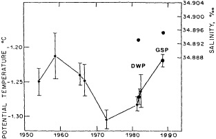
FIGURE 18
Time series of average potential temperature below 2000 m in the Greenland Basin. (From Meincke et al., 1992; reprinted with permission of the International Council for the Exploration of the Sea.)
-
duration and are too short by themselves to permit comment on the question of decadal change in overflow transport (Dickson and Brown, 1994), even though they do appear to emphasize the steadiness rather than the variability of the outflow (Figure 19). A slightly longer perspective is provided by the downstream behavior of tracers, which appears to confirm this impression of steadiness in the overflowing stream. As Schlosser and Smethie point out (1995, in this section), the "age of the deep core between 32°N and 44°N did not change by more than 10% between 1983 and 1990, which implies that the combination of water-mass formation rate, transport, and mixing with adjacent water has been constant to within about ± 10 percent over this time period."
If these points seem unduly critical of current models, they are not intended to be so. There is no doubt that our ability to trace, understand, and simulate these large-amplitude events at high latitudes will open up an important avenue to improved climate prediction. Even if they turn out to be less than cyclic in character, the slow shifts in the ocean-atmosphere system that these events set in motion will still be of use in forecasting effects, and these effects in turn will still be of sufficient significance to make any improvement in prediction worthwhile. The above are merely suggestions for points that future models will have to address—in other words, reasons for model improvement rather than model abandonment. Recent simulations by Weaver (personal communication) appear to support the idea of an invariant THC on decadal time scales.
CONCLUSIONS
-
Although the evidence is circumstantial, there does appear to have been a physically mediated, century-long variation in the exchange of heat and larvae between Iceland and Greenland via the Irminger Current, with major socioeconomic impact.
-
Although it contains periodic elements, the Great Salinity Anomaly is neither a periodic nor a frequently recurring phenomenon. One or possibly two such events are thought to have occurred during this century, and the event we observed in 1968-1982 was driven by a secular change in the winter pressure field at Greenland.
-
Although its proxies clearly reflect the glacial-interglacial signal, the global thermohaline circulation has not yet been demonstrated to vary at decadal time scales. Simulations of the process are not yet adequately realistic in topography, in the role of deep convection (as opposed to Arctic Intermediate Water formation), in the processes that might cap deep convection, and in the periodicity of these processes.
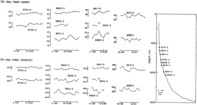
FIGURE 19
Thirty-day means of near-bottom current speed and direction in the Denmark Strait Overflow, taken from successive deployments of instruments set at similar depths on the East Greenland Slope. The "87", "88", and ''89" instruments are from the Angmagssalik Array. The "90" instruments are from equivalent depths on the TTO Array, 160 km upstream. (From Dickson and Brown, 1994; reprinted with permission of the American Geophysical Union.)
Discussion
TALLEY: Is it possible that the Great Salinity Anomaly, singular though it was, could have circled around the basin a few times before dying away?
DICKSON: Our rather poor records of salinity were at their worst just at that point, so we didn't observe that. It's certainly possible— it has a subpolar gyre to go 'round in, and remember Meincke's long studies of the flow across the mid-Atlantic ridge and what gets turned back—but would it make any difference once it's been diluted?
GHIL: Where did you get the periodicities you showed, like the 7-year North Atlantic oscillation?
DICKSON: Well, there were quite a few. The 6.7-year peak you mention was from Rogers. Jerry Namias and I have long talked about another, which is the relationship between conditions at the U.S. eastern seaboard and the high pressures in Greenland. We used air and sea temperature and calculated the seaboard baroclinic gradients for cold and warm groups of years. Then we looked at the storm frequency for those periods, and found an increase along a line up the coast where the gradient was heightened, and a corresponding periodic retraction of the Iceland low.
SARACHIK: You've made the case for the decoupling of convection and genesis and overflow. Would you care to speculate about what can turn off the thermohaline circulation and the production of deep water in the Atlantic?
DICKSON: Knut Aagaard's papers show that it's very delicately poised; the fresh-water flow into the Greenland Sea can stop convection dead. It would take 31 years of the same trend to make a difference at the depth of the Denmark Strait Sill, but during the Ice Age there could have been something quite dramatic. My feeling is that if something so light were formed it would set up a sort of shallow thermohaline circulation. We don't really know yet how intermediate and deep-water formation mesh.
KUSHNIR: It seems possible that very cold temperatures in the central North Atlantic trigger certain atmospheric conditions that pull ice and fresh-water from the Arctic Sea.
MCGOWAN: Bob, was the increased cod population a matter of improved survival or different spatial distribution?
DICKSON: Well, at first people thought it was increased survival because of the improved climate on the West Greenland Banks. But that's not true of haddock, and the haddock catch mirrors the change in cod, so we now think it's a time-varying conveyor belt that relocates larvae.
Observational Evidence of Decadal-Scale Variability of the North Atlantic Ocean
SYDNEY LEVITUS1, JOHN I. ANTONOV1, ZHOU ZENGXI2, HARRY DOOLEY3,
VLADIMIR TSERESCHENKOV4, KONSTANTIN SELEMENOV4, AND ANTHONY F.
MICHAELS5
ABSTRACT
Temperature and salinity time series 27 to 45 years in length are presented for two locations in the North Atlantic. These data are from Ocean Weather Station "C" (52.75°N, 35.5°W), located in the subarctic gyre, and Station "S" (32.16°N, 64.5°W), located in the subtropical gyre. Decadal-scale variability is evident in the deep ocean as well as the upper ocean at these locations. At Station "S", annual mean temperature at 1750 m depth increased by 0.3°C from 1960 to 1990, with salinity also increasing. At OWS "C" annual mean temperature and salinity in the 1,000-to-1,500 m layer increased on the order of tenths of a degree centigrade and 0.02-0.04 psu respectively between 1966 and 1974. From 1975 to 1985 both these parameters decreased by somewhat larger amounts than the earlier increase. At a minimum, these changes indicate that a redistribution of heat and salt have occurred in the North Atlantic Ocean on decadal time scales.
INTRODUCTION
At the beginning of the twentieth century support for research in the field of physical oceanography was justified by the belief that variability of ocean environmental quantities such as temperature and salinity might be responsible for the interannual variability of fisheries. The International Council for the Exploration of the Sea (ICES) was established at this time (1902) for the purpose of coordinating such studies on an international scale. The governments of the various north European countries that founded ICES recognized the requirement to undertake such studies multi-nationally. Many of the founders of the field of physical oceanography, such as V. W. Ekman and M. Knudsen, were scientific members of this organization.
One of the earliest descriptions of interannual variability
was provided by Helland-Hansen and Nansen (1909), who observed that the flow of North Atlantic water into the Norwegian Sea exhibited interannual variability. Because of a lack of appropriate data, due in part to the expense of oceanographic measurement programs and the disruptions caused by the two world wars, studies describing temporal variability of open ocean conditions during the twentieth century are relatively few. The importance of determining the role of the ocean as part of the earth's climate system has promoted greater involvement of international and intergovernmental scientific organizations in examining the issue of temporal variability of the world ocean.
The World Climate Research Program published results (WCRP, 1982) from a meeting convened to discuss existing long-term time series of oceanographic parameters, particularly temperature and salinity but also biological and chemical parameters. The Intergovernmental Oceanographic Commission is publishing analyses (IOC, 1983, 1984, 1986, 1988) of time series of oceanographic parameters "to demonstrate the importance and usefulness of time series data to the understanding of oceanic and atmospheric processes." Levitus (1989a) briefly reviews some of these studies.
We have analyzed temperature and salinity time-series data at two locations in the North Atlantic Ocean—Ocean Weather Station "C" (OWS "C"), located in the subarctic gyre, and Station "S", located in the subtropical gyre. We present our results in the following sections. In order to place these time series in oceanographic context, which will assist in interpretation, we present Figures 1-3. These show the climatological annual mean distribution of temperature and salinity at depths of 100 m, 1500 m, and 1750 m, respectively, for the North Atlantic Ocean; the locations of OWS "C" and Station "S'' are marked by the letters C and S. These climatological distributions represent the output from objective analyses of climatological means over 1° squares of all temperature and salinity data in the files of the National Oceanographic Data Center (NODC), Washington, D.C. as of December, 1988. The analysis techniques used are the same as those described by Levitus (1982). OWS "C" was located in the vicinity of the Ocean Polar Front (OPF), an upper-ocean feature associated with the North Atlantic Current. In the deeper layers OWS "C" occupies a location affected by the properties of deep water formed in the Labrador Sea (Talley and McCartney, 1982). Station "S" is located near Bermuda just south of the Gulf Stream recirculation.
VARIABILITY AT OCEAN WEATHER STATION "C"
Variability of Upper Ocean Thermal Structure at OWS "C"
Ocean Weather Station "C" was located in the North Atlantic at approximately 52.75°N, 35.5°W. For the period
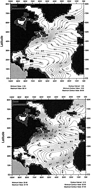
FIGURE 1
Climatological distribution of annual mean temperature (upper panel, in °C) and annual mean salinity (lower panel, in psu) at a depth of 100 m for the North Atlantic Ocean. "C" indicates the location of Ocean Weather Station "C", and "S" the location of Station "S".
1946-1964 OWS "C" was occupied by ships of the U.S. Coast Guard. During that period, only temperature profiles made using mechanical bathythermographs (MBTs) were taken. From 1964 through 1974, hydrographic casts (reversing thermometers to measure temperature and seawater samples gathered for salinity determinations) were made, as
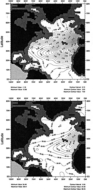
FIGURE 2
Climatological distribution of annual mean temperature (upper panel, in °C) and annual mean salinity (lower panel, in psu) at a depth of 1500 m for the North Atlantic Ocean. "C" indicates the location of Ocean Weather Station "C", and "S" the location of Station "S''.
well as MBT casts in some years. Hannon (1979) described some results of analyses of these hydrographic data. From 1975 through 1990, research ships from the Former Soviet Union (FSU) occupied this ocean weather station. They took Nansen casts and conductivity-temperature-depth (CTD) profiles, in addition to some MBT profiles. Some
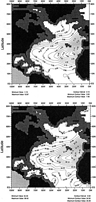
FIGURE 3
Climatological distribution of annual mean temperature (upper panel, in °C) and annual mean salinity (lower panel, in psu) at a depth of 1750 m for the North Atlantic Ocean. "C" indicates the location of Ocean Weather Station "C", and "S" the location of Station "S".
of the FSU data for OWS "C" were available only in the form of daily means. Therefore, we have averaged all data to form daily means before forming other averages so as to use all data in a consistent manner.
Figure 4a displays the time series of annual mean temperature at a 100 m depth at OWS "C" for the period 1947-
1989. Individual monthly means are computed as the average of all daily mean profiles in each month. Each annual mean is computed as the average of the available monthly means for each year. All years plotted in Figure 4a had at least one monthly mean for each of the four seasons. The vertical bars centered at each annual mean represent ± 1 standard error of the monthly means in each year about the annual mean.
There are two prominent features of this series. The first is the approximately decadal-scale oscillation of about 2°C magnitude, with peaks occurring in 1956, 1965, and 1979. The years for which we have both station data and MBT data indicate good agreement between these two different sets of measurements, and give us confidence in the accuracy and representativeness of annual mean MBT data that have been averaged as we have done. Although the accuracy of any individual MBT measurement is an order of magnitude less than that of a reversing thermometer measurement (0.2°C versus 0.02°C), the accuracy of monthly and annual mean values is increased by averaging many observations. Figure 4a clearly demonstrates that the signal-to-noise ratio
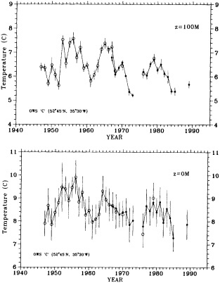
FIGURE 4
Time series of annual mean temperature (°C) from OWS "C" data. The vertical bars centered at each annual mean data point represent ± 1 standard error of the monthly means for that year about the annual mean for that year. Upper panel, at a depth of 100 m; lower panel, at the sea surface.
is small enough that averaged MBT data are adequate to define the observed signal (2°C peak-to-trough difference in annual mean temperature).
The monthly mean data used in Figure 4a was derived from both MBT and station daily means. The MBT data was available from 1946 through 1981. During the 1947-1954 period and again in 1960-1967, measurements were taken quite frequently, sometimes daily. During the 1970s relatively few observations were made, although a couple of times the annual frequency again reached 150 or higher (as it had been during 1955-1959). The station data, which covers 1964 through 1990, reflects reasonably frequent observations (again, about 150 per year) for the period 1967-1973, and then near-daily readings for 1976-1985. Both the MBT data and the station observations were scattered fairly evenly throughout the year.
Figure 4b shows the time series of annual mean sea surface temperature (SST) for OWS "C". The same features observed at 100 m occur at the sea surface. To provide further evidence of the existence of both the downward trend and the decadal-scale oscillation, Figure 5 presents
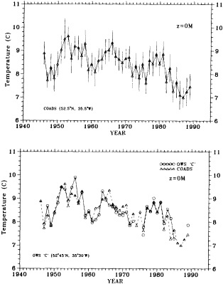
FIGURE 5
Time series of annual mean temperature (°C) at 52.5°N, 35.5°W at the sea surface. The vertical bars centered at each annual mean data point represent ± 1 standard deviation of the monthly means for that year about the annual mean for that year. Upper panel, COADS data; lower panel, COADS data and OWS "C" time series data set.
the time series of annual mean temperature at 52.5°N, 35.5°W taken from objective analyses of SST observations from the Comprehensive Ocean Atmosphere Data Set (COADS) of surface marine observations (Woodruff et al., 1987). The COADS data have been gridded and analyzed using the same procedures described by Levitus (1982) as part of a joint project with A. Da Silva of the University of Wisconsin. (We emphasize that the OWS "C" time series are averages of the data taken by ships at the OWS "C" location.) Figure 5a shows the annual mean temperature at this grid point as computed from the 12 monthly fields of objectively analyzed SST data for each year. Figure 5b shows the annual mean time series for the OWS "C" surface data and the COADS data time series plotted together to facilitate comparison. Some differences exist between these two data sets, but the comparison indicates that both data sets display the same negative trend as well as the same decadal-scale oscillation. The year of maximum temperature of the decadal-scale oscillation in each series may differ by 1 to 3 years in each figure. We attribute this to differences in data density and differences in the way these annual means have been computed. The decreasing SST of the North Atlantic Ocean over this time period has been described in previous studies (e.g., Folland et al., 1984).
To further describe the temporal variability at this location, Figure 6 presents the time-depth temperature field at OWS "C" over the 0-125 m depth range. This figure makes it very clear that both the negative trend and decadal-scale oscillations noted in Figures 4 and 5 extend coherently over the upper water column. There is no phase propagation with depth of the interannual variations.
Beginning in the mid-1960s, very-low-salinity water was observed at various locations along the periphery of the subarctic gyre of the North Atlantic. Dickson et al. (1988) have suggested that this low-salinity (and relatively cold) water advected out of the Arctic Ocean into the subarctic gyre of the North Atlantic and circulated around this gyre.
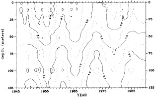
FIGURE 6
Annual mean temperature (°C) as a function of depth and time, based on the OWS "C" time series data.
They identified changes in salinity that occurred at OWS "C" in the 1970s as being associated with the "Great Salinity Anomaly" (GSA). Levitus (1989b) also presented evidence for this. Dooley et al. (1984), however, suggested that the changes at OWS "C" were associated with horizontal movement of the OPF. The fact that several oscillations have occurred in the temperature data at OWS ''C" suggests that the OPF might be shifting its axis. It does not seem likely to us that the cold, fresh-waters of the GSA have traveled around the subarctic more than once. Further examination of the historical data will be required to test these different hypotheses. Perhaps both phenomena are responsible to some degree for the decadal-scale variability at OWS "C". Quite possibly the GSA was a phenomenon independent of the process responsible for the oscillations we describe in Figures 4 to 6.
To place the variability described by Figure 6 in perspective, Figure 7 presents the climatological annual cycle of OWS "C" upper-ocean temperature data. At a 100 m depth the annual range of temperature is approximately 1.8°C. A clear propagation of phase with depth is observed.
Variability of Deep-Ocean Temperature and Salinity at OWS "C"
To document the variability of deep ocean conditions at OWS "C," Figure 8 presents time series of temperature and salinity for the 1964-1990 period. Again, all data for the 1964-1973 period are U.S. Coast Guard observations (Hannon, 1979), and the 1975-1990 data are Russian observations. While only a few observations were available for the
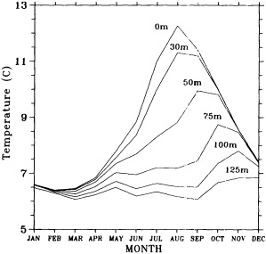
FIGURE 7
Climatological annual cycle of temperature (°C) based on the OWS "C" data series.
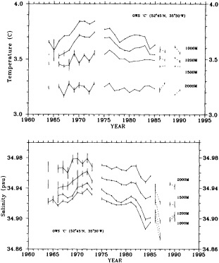
FIGURE 8
Time series of deep ocean temperature (upper panel, in °C) and deep ocean salinity (lower panel, in psu) at OWS "C" location.
periods 1964-1975 and 1986-1990, readings were taken almost daily from mid-1975 through 1985.
Figure 8 shows that annual mean temperature increased by 0.25°C between 1964 and 1971 at a depth of 1000 m, which is consistent with the results of Levitus (1989c) and Antonov (1990). Temperature then decreased a total of 0.20°C by 1984 at this same depth. The magnitude of these temperature changes decreased with increasing depth. Comparison of the two panels of Figure 8 reveals that, in general, changes in salinity were positively correlated with temperature changes at these depths. During the 1965-1972 period, the salinity data at the 1000 m level exhibit a positive trend that led to an increase of about 0.02 psu in the annual mean. After 1972 the trend reversed sign, and salinity decreased by 0.05 psu by 1984. There is some evidence of a further decrease in salinity during the post-1985 period. The amount of data available in this period is limited, however, so we choose not to emphasize this portion of the record. Data do exist for this period, and these series will be updated in a future work. One important feature to note is that the salinity at a depth of 2000 m shows a decrease beginning in 1975, but there is no corresponding change in temperature at this depth.
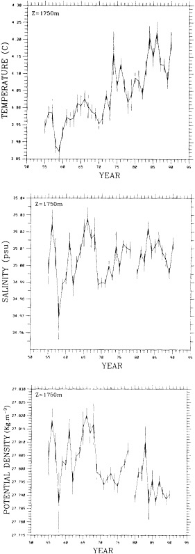
FIGURE 9
Time series at 1750 m depth at Station "S". Upper panel, temperature (°C); middle panel, salinity (PSU); lower panel, potential density (kg m-3).
VARIABILITY OF DEEP-WATER TEMPERATURE AND SALINITY AT THE STATION "S" LOCATION
Ocean Weather Station "S", located off Bermuda (32.16°N, 64.5°W), was established in 1954 through the efforts of Henry Stommel (WHOI and BBSR, 1988). Beginning in 1954, hydrographic profiles have been made on a monthly or semimonthly basis. This time series is one of the longest in existence for an oceanographic quantity, particularly for the deep ocean.
The work of Roemmich (1985) presents some of the most recent analyses of the data from this time series. Roemmich found evidence of decadal-scale trends in the deep ocean temperature off Bermuda. He smoothed the annual mean values of his time series with a 5-year running mean, however, and presented no evidence of decadal-scale oscillations or interannual variability.
We have used the data from the OWS "S" series, as well as other hydrographic data taken within a one-half degree radius of this location, and present here the results of an analysis of the resulting combined data series at 1750 m depth. Measurements at OWS "S" were made fairly regularly for the entire 1954-1990 period, mostly about 4 per month, with occasional periods of heavier sampling.
Figure 9 shows the time series of annual mean temperature, salinity, and potential density at a depth of 1750 m for the 1955-1990 period. As in our earlier figures, the vertical bars centered at each annual mean data value represent the range of ± I standard deviation of the monthly means for each year about the annual mean. The dominant feature in the temperature series is the positive trend during the 1959-1990 period. This trend resulted in a net warming of about 0.3°C over a 30-year period. Superimposed on this trend are decadal-scale oscillations with a range of about 0.10°C to 0.15°C. To better describe these oscillations, we have detrended the 1959-1990 portion of the time series. The warmer portions of these oscillations are centered about the years 1965, 1975, and 1985. Figure 9b shows the salinity series at 1750 m. The minimum salinity of this series occurred in 1958, one year earlier than the temperature minimum. There is a small positive linear trend in salinity. In addition, the decadal-scale oscillations of temperature have counterparts in the salinity record. A positive correlation is observed between the two detrended parameters during the 1960s and 1970s, but it is less strong in the 1980s.
CONCLUSION
The time-series results presented in this paper indicate that statistically significant decadal-scale changes of temperature and salinity have occurred in both the subarctic and the subtropical gyres of the North Atlantic Ocean. These time-series results further characterize the variability of the North Atlantic described in a series of scientific papers published over the last 12 years. These papers include, but are certainly not limited to, the works of Lazier (1980, 1988, 1995), Brewer et al. (1983), Dickson et al. (1988), Dooley et al. (1984), Mysak (1995), Roemmich (1985), Roemmich and Wunsch (1984), Swift (1984a, 1985), Taylor (1983), Levitus (1989a,b,c; 1990), Antonov (1990), and Antonov and Groisman (1988).
Several statements can be made on the basis of the results of this study and the work of others mentioned above:
-
At a minimum, oceanographers have succeeded in documenting the large-scale redistributions of heat and salt in the North Atlantic Ocean that occurred in the 19461990 period.
-
The decadal-scale variability of the North Atlantic Ocean we have described may represent the ocean component of decadal-scale interactions between the various parts of the earth's ocean-atmospheric-cryosphere climate system. The existence of such variability provides the observational basis for future diagnostic and modeling studies.
-
Any program for monitoring the world ocean in order to determine its role in the earth's climate system must include an examination of these changes in the deep ocean.
ACKNOWLEDGMENTS
Funding for the work described in this paper was provided by the NOAA Climate and Global Change Program and the NOAA Earth Sciences Data and Information Management Program. This paper is BBSR Contribution No. 1349.
Commentary on the Paper of Levitus et al.
JOHN R.N. LAZIER
Bedford Institute of Oceanography
Dr. Levitus and his co-authors suggest that the low-frequency temperature variations in the upper layers at Ocean Weather Ship (OWS) Charlie may be related to the lower-than-normal salinity that appeared in the subpolar gyre between 1968 and 1978. To explore this possibility I wish to examine some features of this phenomenon, which has come to be known as the Great Salinity Anomaly (Dickson et al., 1988).
In the latter half of the 1960s the salinity in the Iceland Sea became anomalously fresh (Dickson et al., 1975). Subsequently, water of lower-than-normal salinity was observed at various stations around the subpolar gyre. Taken together, these observations led Dickson et al. (1988) to propose that all these signals were due to a single pulse of low-salinity water moving around the subpolar gyre. They demonstrated that the low-salinity water moved out of the Iceland Sea into the North Atlantic Ocean via the East Greenland Current, and thence to the Labrador Sea (1972), the Labrador Current (1971-1972), OWS Charlie (1974), the Faeroe-Shetland Channel (1976), the Barents Sea (1978), and the Greenland Sea (1981-1982). The average rate of advance over the 14-year circuit was approximately 0.03 m s-1. The total salt deficit was estimated to be 72 × 1012 kg along the Labrador shelf, but by the time the anomaly moved north through the Faeroe-Shetland Channel into the Barents and Greenland Seas it was reduced to about 47 × 1012 kg.
The decrease in salinity caused by the passage of the anomaly is illustrated in Figure 1. Here the time series of salinity averaged over the upper 800 m at OWS Charlie is presented, along with eight similar values I calculated for September of the years 1966 to 1973 at OWS Bravo. The latter have been displaced along the time axis; the OWS Bravo values were actually obtained three years earlier than the year indicated.
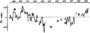
FIGURE 1
The 0-800 m average salinity at OWS Charlie (solid line), adapted from Dickson et al. (1988), and at OWS Bravo (circles) for September of the years 1966 to 1976. The data for OWS Bravo have been plotted 3 years late to match the variation at OWS Charlie.
The salinity variation through the years is clearly similar in magnitude at the two weather ships, but the minimum occurs at OWS Bravo about three years before it occurs at OWS Charlie, which supports the conclusion of Dickson et al. (1988) that the low-salinity water could have moved from OWS Bravo to Charlie. Farther east, the salinity variation through these years is similar to that at the weather ships. This is illustrated by the five-year running mean of the surface salinity in Rockall Channel shown in Figure 2. According to Dickson et al. (1988), the decrease in the Rockall Channel of about 0.08 between the late 1960s and 1976 occurs about 9 months after the decrease at OWS Charlie, which fits well with their advection hypothesis.
It is unfortunate that Levitus et al. were unable to present the salinity data for OWS Charlie to compare with the temperature data, since the Great Salinity Anomaly is noted for a change in salinity rather than a change in temperature. The temperature records in their Figures 4, 5, and 6 do exhibit minima in the mid-1970s at the same time that the salinity is minimum in my Figure 2; however, the temperature data also indicate minima of similar magnitude in the early 1960s and mid-1980s that do not appear to be connected to the Great Salinity Anomaly or any other large-scale salinity minimum.
Another possibility raised by Levitus is that the low salinity signal at OWS Charlie could be due to long-period horizontal displacements of the water masses, which would bring water of lower salinity into the region of OWS Charlie.
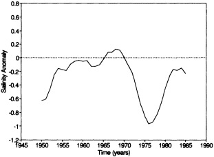
FIGURE 2
Five-year running mean of the winter sea surface salinity anomaly in Rockall Channel, adapted from Ellett and Edelsten (1983) and Ellett (pers. Comm.).
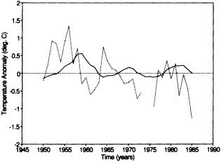
FIGURE 3
The annual average sea surface temperature anomaly (dotted line), adapted from Levitus's Figure 5, and the 5-year running mean of the winter sea surface temperature anomaly in Rockall Channel (solid line), adapted from Ellett and Edelsten (1983) and Ellett (pers. Comm.).
If this is the mechanism for the variation at OWS Charlie it should also be the mechanism for the variations at OWS Bravo, Rockall Channel, and the other places where the anomaly signal has been observed. At 50°N 51.5°W, OWS Bravo is near the center of the cyclonic gyre that dominates the circulation of the Labrador Sea. There are no horizontal gradients that could be moved to lower the salinity of the top 800 m of the water column without drastically altering the dynamics of the sea, and no such alteration has been observed. This is also true in the Rockall Channel, so the interpretation of Dickson et al. (1988), an advecting anomaly, fits more comfortably with the observations.
To look further at the relationship between OWS Charlie and the Rockall Channel I have prepared Figure 3, which shows the sea-surface temperature variations at these two points. The data for OWS Charlie is from Dr. Levitus's Figure 5, and the surface temperature anomaly (for winter) in the Rockall Channel is from Ellett and Edelsten (1983) and Ellett (pers. comm.). The amplitudes of the variations at OWS Charlie are larger than at Rockall; this is in part because they are based on annual averages, while those at Rockall are 5-year running means. The interesting feature is that in each record there is a variation of about 10 years' period that occurs at Rockall roughly 5 years later than at OWS Charlie, whereas Dickson et al. (1988) demonstrated that the Great Salinity Anomaly moved from OWS Charlie to Rockall Channel in 9 months. If we assume that the temperature variations at OWS Charlie are connected to the Great Salinity Anomaly, we are then faced with the problem of explaining why the variations due to salinity move to Rockall Channel five times faster than those due to temperature.
Discussion
GOODRICH: Was there a demonstrable air-temperature signal associated with the presumably colder, fresher water of the Great Salinity Anomaly?
LEVITUS: I'm not sure. But there certainly was for this decadal-scale oscillation and for the decreasing trend.
GROISMAN: If I had only two stations on land, I wouldn't dare claim that I was seeing interdecadal variability in surface temperature. If your two ocean stations are near strong temperature fronts, how can you be sure from those observations that long-term changes aren't the result of a 200-km shift east or west in such a front?
LEVITUS: We're mostly trying to document the variability, and we have confirmation from other data sets for that. There may be some contribution from front changes in the upper ocean, but I really don't think that they can explain the horizontal shifts in the deep ocean that we're seeing at OWS "C".
MOREL: I have two questions. First, can we associate these demonstrated changes in the ocean that are on decadal or longer time scales with actual changes in climate, such as atmospheric circulation? Ocean variability would not qualify as climate research otherwise. And second, could you suggest a practical sampling strategy for a global climate—not just ocean-—observing system?
LEVITUS: I think that what's most important in connection with both your questions is bringing together the huge amount of data that already exists. We at NOAA are digitizing data from the U.S., Europe, and Russia. We are seeing a decadal-scale oscillation in the COADS, subsurface, and SAT data, but it will take several years before we can evaluate all this historical data and design a better global observing system.
One of the important things we've already learned is that we need long-term commitments if we are to look at long-time-scale problems. As we saw at the Panulirus station, you can have 10 years with no changes and suddenly see very large changes. The assurance of continuing financial support is as essential as good design for an observing system.
MYSAK: In response to Pierre Morel's first question, I wanted to point out that Rosanne D'Arrigo's reconstructions of tree rings
from Labrador, Newfoundland, and Nova Scotia very clearly reflect cooling at the time of the GSA.
DESER: And I'd like to emphasize that the decadal SST variability is clearly reflected in the atmosphere as high as the 50-mb level. It's influencing storm tracks, and in fact you can see it in rainfall over western Ireland.
BRYAN: This question of why we should measure deep-ocean temperature when the atmosphere can respond only to SST is a long-standing one. I think there are two reasons. The first is that the deep-sea signals are signatures of past events that may be important for unraveling both the mechanism and the magnitude of the exchanges of heat between the ocean and atmosphere. The second is that unless the temperature changes we see are perfectly compensated for by salinity, the thermohaline circulation is responding to the pressure fields within the ocean itself, and those circulation changes do have a large effect on SST in areas of strong currents.
GHIL: Pierre, I really think we can safely assume that the ocean is part of the climate system. Also, it seems to me that suggesting that all the ocean is good for is giving you SSTs is like saying that all the atmosphere is useful for is heat fluxes.
MOREL: Many phenomena in the ocean, like the tides, are not part of climate, any more than rainbows in the atmosphere are.
GOOS, as currently defined, covers everything that can be measured in the ocean, which is why I was asking about a sampling strategy. I feel that a cause-and-effect relationship between decadal variability in the ocean and decadal variability in the atmosphere needs to be shown before we can consider the former a climate phenomenon.
MARTINSON: That's odd; I would have said that the atmospheric moisture reflected in rainbows was part of climate.
ROOTH: Getting serious, now, the temperature anomalies on a 10-year time scale at OWS "C" mean that you can have fairly substantial changes in moist static energy at the surface. Being an old cloud-physics man, I think that we need to look at that, not just dry energy, as we try to feed ocean temperature back into climate. As for location of observation stations, we do need to understand the processes in the deep in the Atlantic, because of the deep-water formation and the convective effects, which involve large temperature differences. The deep circulation in the Pacific appears to be much less important to understanding what goes on at the surface on decadal time scales.
LEHMAN: It seems to me that I've been hearing some of the first evidence connecting ocean surface variability with real changes in the interior. I think modelers should really be homing in on this evidence of surface-to-deep-ocean coupling that directly implicates thermohaline circulation in the variability of the surface.
Ocean Observations Reference List
Aagaard, K., and E.C. Carmack. 1989. On the role of sea ice and other fresh-water in the Arctic circulation. J. Geophys. Res. 94:14485-14498.
Aagaard, K., J.H. Swift, and E.C. Carmack. 1985. Thermohaline circulation in the Arctic Mediterranean seas. J. Geophys. Res. 90:4833-4846.
Alexander, R.C., and R.L. Mobley. 1976. Monthly average sea-surface temperatures and ice-pack limits on a 1° global grid. Mon. Weather Rev. 104:143-148.
Antonov, J. 1990. Recent climatic changes of the vertical thermal structure of the North Atlantic Ocean and the North Pacific Ocean. Meteor. Gidrol. 4:78-87 (in Russian).
Antonov, J., and P. Groisman. 1988. Seawater temperature change below the seasonal thermocline in the North Atlantic. Meteor. Gidrol. 3:57-63 (in Russian).
Barnett, T.P. 1990. Recent changes in sea level: A summary. In Sea-Level Change. National Research Council, Studies in Geophysics, National Academy Press, Washington, D.C., pp. 37-51.
Bayer, R., P. Schlosser, G. Bönisch, H. Rupp, F. Zaucker, and G. Zimmek. 1989. Performance and blank components of a mass spectrometric system for routine measurement of helium isotopes and tritium by the 3He ingrowth method. Sitzungsber. Heidelb. Akad. Wissensch., Math. Naturwiss. Kl., Jahrgang 1989, 5, Springer-Verlag, pp. 241-279.
Bjerknes, J. 1964. Atlantic air-sea interaction. Adv. Geophys. 10:1-82.
Blindheim, J., and H.R. Skjoldal. 1993. Effect of climatic change on the biomass yield of the Barents Sea, Norwegian Sea and West Greenland large marine ecosystems. In Large Marine Ecosystems. K. Sherman, M. A. Lewis, and B. D. Gold (eds.). American Association for the Advancement of Science, Washington, D.C., pp. 185-198.
Bottomley, M., C.K. Folland, J. Hsiung, R.E. Newell, and D.E. Parker. 1990. Global Ocean Surface Temperature Atlas (GOSTA). Joint Project of the Meteorological Office, Bracknell, U.K., and the Massachusetts Institute of Technology. HMSO, London, 20iv pp. and 313 plates.
Bradley, R.S., and J. England. 1978. Recent climatic fluctuations of the Canadian high Arctic and their significance for glaciology. Arct. Alp. Res. 10:715-731.
Brewer, P.G., W. S. Broecker, W.J. Jenkins, P.B. Rhines, C.G. Rooth, J.H. Swift, T. Takahashi, and R.T. Williams. 1983. A climatic freshening of the deep North Atlantic (north of 50°N), over the past 20 years. Science 222:1237-1239.
Broecker, W.S., and T.-H. Peng. 1984. Gas exchange rates between air and sea. Tellus 26:21-35.
Broecker, W.S., T.-H. Peng, G. Östlund, and M. Stuiver. 1985a. The distribution of bomb radiocarbon in the ocean. J. Geophys. Res. 90:6953-6970.
Broecker, W.S., D.M. Peteet, and D. Rind. 1985b. Does the ocean-atmosphere system have more than one stable mode of operation? Nature 315:21-26.
Brummer, B., E. Augstein, and H. Riehl. 1974. On the low-level wind structure in the Atlantic trade. Quart. J. Roy. Meteorol. Soc. 100: 109-121.
Bryan, K., and R. Stouffer. 1991. A note on Bjerknes' hypothesis for North Atlantic variability. J. Mar. Sys. 1:229-241.
Bu, X. and M.J.W. Warner. 1995. Solubility of Chlorofluorocarbon 113 in water and seawater. Deep-Sea Res. 42:1151-1161.
Buch, E., and H.H. Hansen. 1988. Climate and cod fishery at West Greenland. In Long-Term Changes in Marine Fish Populations. T. Wyatt and M.G. Larraneta (eds.). Instituto de Investigaciones Marinas, Vigo, Spain, pp. 345-364.
Bullister, J.L., and R.F. Weiss. 1983. Anthropogenic chlorofluoromethanes in the Greenland and Norwegian Seas. Science 221:265-268.
Bullister, J.L., and R.F. Weiss. 1988. Determination of CCl3F and CCl2F2 in seawater and air. Deep-Sea Res. 35:839-853.
Cardone, V.J., J.G. Greenwood, and M.A. Cane. 1990. On trends in historical marine wind data, J. Climate 3:113-127.
Carter, W.E., D.G. Aubrey, T. Baker, C. Boucher, C. LeProvost, D. Pugh, W. Peltier, M. Zumberge, R. Rapp, B. Schutz, K. Emery, and D. Enfield. 1989. Geodetic Fixing of Tide Gauge Bench Marks. Technical Report WHOI-89-31, Woods Hole Oceanographic Institution.
Cattle, H. 1985. Diverting Soviet rivers: Some possible repercussions for the Arctic Ocean. Polar Res. 22:485-498.
Chapman, W.L., and J.E. Walsh. 1991. Long-range prediction of regional sea ice anomalies in the Arctic. Wea. Forecast. 6:271-288.
Charles, C.D., and R.G. Fairbanks. 1992. Evidence from Southern Ocean sediments for the effect of North Atlantic deep-water flux on climate. Nature 355:416-419.
Chemical Manufacturers Association, Fluorocarbon Program Panel. 1983. World production and release of chlorofluorocarbons 11 and 12 through 1981. FPP 83-F, Washington, D.C.
Cheney, R.E., W.J. Emery, B.J. Haines, and F. Wentz. 1991. Recent improvements in Geosat altimeter data. EOS, Trans. AGU 72:577-580.
Clarke, R.A. 1984. Changes in the western North Atlantic during the decade beginning in 1965. C.M. 1984/Gen:17, International Council for the Exploration of the Sea, Copenhagen, 7 pp. (mimeo).
Clarke, R.A., and A.R. Coote. 1988. The formation of Labrador Sea Water. Part III: The evolution of oxygen and nutrient concentration. J. Phys. Oceanogr. 18:469-480.
Clarke, R.A., and J.C. Gascard. 1983. The formation of Labrador Sea Water. Part I: Large-scale processes. J. Phys. Oceanogr. 13:1764-1778.
Clarke, R.A., J.H. Swift, J.L. Reid, and K.P. Koltermann. 1990. The formation of Greenland Sea Deep Water: Double diffusion or deep convection? Deep-Sea Res. 37:1385-1424.
Clarke, W.B., W.J. Jenkins, and Z. Top. 1976. Determination of tritium by mass spectrometric measurement of 3He. Int. J. Appl. Rad. Isotopes 27:515-522.
Colman, A.W. 1992. Development of worldwide marine data eigenvectors since 1985. CRTN 28, 26 pp. (Available from the National Meteorological Library, London Road, Bracknell, Berks, RG12 2SZ, U.K.)
Colony, R., and A.S. Thorndike. 1984. An estimate of the mean field of Arctic sea ice motion. J. Geophys. Res. 89:10623-10629.
Craig, H., and D. Lal. 1961. The production of natural tritium. Tellus 13:85-105.
Cunnold, D.M., R.G. Prinn, R.A. Rasmussen, P.G. Simmonds, F.N. Alyea, C.A. Cardelino, A.J. Crawford, P.J. Fraser, and R.D. Rosen. 1986. Atmospheric lifetime and annual release estimates for CFCl3 and CF 2Cl2 from 5 years of ALE data. J. Geophys. Res. 91:10797-10817.
Danke, L. 1967. Erster bericht über kabeljaumarkierung 1964 bis 1966 bei Labrador. Fischerie Forsch. 5(1):87-91.
Darby, M.S., and L.A. Mysak. 1993. A Boolean delay equation model of an interdecadal Arctic climate cycle. Climate Dynamics 8:241-246.
Delworth, T.L., S. Manabe, and R.J. Stouffer. 1993. Interdecadal variations of the thermohaline circulation in a coupled ocean-atmosphere model. J. Climate 6:1993-2011.
Deser, C., and M.L. Blackmon. 1993. Surface climate variations over the North Atlantic Ocean during winter: 1900-1989. J. Climate 6:1743-1753.
Deutsches Hydrographisches Institut. 1950. Atlas of ice conditions in the North Atlantic Ocean and general charts of the ice conditions of the North and South Polar regions. Deutsches Hydrog. Inst. Publ. No. 2335, Hamburg, 24 pp. and 34 colored charts (in German).
Dickson, R.R. 1995. The local, regional, and global significance of exchanges through the Denmark Strait and Irminger Sea. In Natural Climate Variability on Decade-to-Century Time Scales. D.G. Martinson, K. Bryan, M. Ghil, M.M. Hall, T.R. Karl, E.S. Sarachik, S. Sorooshian, and L.D. Talley (eds.). National Academy Press, Washington, D.C.
Dickson, R.R., and J. Brown. 1994. The production of North Atlantic Deep Water: Sources, rates and pathways . J. Geophys. Res. 99(C6):12319-12341.
Dickson, R.R., and J. Namias. 1976. North American influences on the circulation and climate of the North Atlantic sector. Mon. Weather Rev. 104:1255-1265.
Dickson, R.R., H.H. Lamb, S.-A. Malmberg, and J.M. Colebrook. 1975. Climatic reversal in the northern North Atlantic. Nature 256:479-482.
Dickson, R.R., S.-A. Malmberg, S.R. Jones, and A.J. Lee. 1984. An investigation of the earlier great salinity anomaly of 191014 in waters west of the British Isles. C.M. 1984/Gen:4, International Council for the Exploration of the Sea, Copenhagen, 15 pp. + 15 figs. (mimeo).
Dickson, R.R., J. Meincke, S.-A. Malmberg, and A.J. Lee. 1988. The "Great Salinity Anomaly" in the northern North Atlantic, 1968-1982. Progr. Oceanogr. 20:103-151.
Doney, S.C., D.M. Glover, and W.J. Jenkins. 1992. A model function of the global bomb tritium distribution in precipitation, 1960-1986. J. Geophys. Res. 97:5481-5492.
Dooley, H.D., J.H.A. Martin, and D.J. Ellett. 1984. Abnormal hydrographic conditions in the northeast Atlantic during the 1970s. Rapp. P.-v. Rëun. Cons. Int. Explor. Mer 185:179-187.
Douglas, B.C. 1991. Global sea level rise. J. Geophys. Res. 96:6981-6992.
Douglas, B.C. 1992. Global sea level acceleration. J. Geophys. Res. 97:12699-12706.
Douglas, B.C. 1995. Long-term sea-level variation. In Natural Climate Variability on Decade-to-Century Time Scales. D.G. Martinson, K. Bryan, M. Ghil, M.M. Hall, T.R. Karl, E.S. Sarachik, S. Sorooshian, and L.D. Talley (eds.). National Academy Press, Washington, D.C.
Dreisigacker, E., and W. Roether. 1978. Tritium and Sr-90 in North Atlantic surface water. Earth Planet. Sci. Lett. 38:310-312.
Druffel, E.M., and T.W. Linick. 1978. Radiocarbon in annual coral rings of Florida. Geophys. Res. Lett. 5:913-916.
Ellett, D.J., and D.J. Edelsten. 1983. Hydrographic conditions in the central Rockall Channel during 1980. Ann. Biol. 37:63-66.
Emery, K.O., and D.G. Aubrey. 1991. Sea Levels, Land Levels, and Tide Gauges. Springer-Verlag, New York.
Fine, R., and R.L. Molinari. 1988. A continuous deep western boundary current between Abaco (26.5°N) and Barbados (13°N). Deep-Sea Res. 35:1441-1450.
Fissel, D.B., and H. Melling. 1990. Interannual variability of the oceanographic conditions in the southeastern Beaufort Sea. Can. Contr. Rep. Hydro. Ocean Sci. No. 35, 102 pp. (plus 6 microfiches).
Fleming, G.H., and A.J. Semtner, Jr. 1991. A numerical study of interannual ocean forcing on Arctic sea ice. J. Geophys. Res. 96:4589-4603.
Folland, C.K. 1991. Sea temperature bucket models used to correct historical sea surface temperature data in the Meteorological Office. CRTN 14, 29 pp. (Available from the National Meteorological Library, London Road, Bracknell, Berks, RG12 2SZ, U.K.)
Folland, C.K., and D.E. Parker. 1992. The instrumental record of surface temperature: How good is it and what can it tell us about climate change and variability? In Proceedings, Fifth International Meeting on Statistical Climatology and Twelfth American Meteorological Society Conference on Probability and Statistics in the Atmospheric Sciences (Toronto). American Meteorological Society, Boston, Mass., pp. J1-J6.
Folland, C.K., and D.E. Parker. 1995. Correction of instrumental biases in historical sea surface temperature data. Quart. J. Roy. Meteorol. Soc. 121:319-367.
Folland, C.K., D.E. Parker, and F.E. Kates. 1984. Worldwide marine temperature fluctuations 1856-1981. Nature 310:670-673.
Folland, C.K., D.E. Parker, M.N. Ward, and A.W. Coleman. 1986a. Sahel rainfall, northern hemisphere circulation anomalies and the worldwide sea surface temperature changes. Memorandum 7a, Long Range Forecasting Climate Research, Meteorological Office, Bracknell, U.K. 49 pp.
Folland, C.K., T.N. Palmer, and D.E. Parker. 1986b. Sahel rainfall and worldwide sea temperatures. Nature 320:602-607.
Folland, C.K., T.R. Karl, and K.Ya. Vinnikov. 1990. Observed climate variations and change. In Climate Change: The IPCC Scientific Assessment. J.T. Houghton, G.J. Jenkins, and J.J. Ephraums (eds.). Prepared for the Intergovernmental Panel on Climate Change by Working Group I. WMO/UNEP, Cambridge University Press, pp. 195-238.
Folland, C.K., T.R. Karl, N. Nicholls, B.S. Nyenzi, D.E. Parker, and K.Ya. Vinnikov. 1992. Observed climate variability and change. In Climate Change 1992: The Supplementary Report to the IPCC Scientific Assessment. J.T. Houghton, B.A. Callander, and S.K. Varney (eds.). Prepared for the Intergovernmental Panel on Climate Change by Working Group I. WMO/UNEP, Cambridge University Press, pp. 135-170.
Folland, C.K., R.W. Reynolds, M. Gordon, and D.E. Parker. 1993. A study of six operational sea surface temperature analyses. J. Climate 6:96-113.
Fridriksson, A. 1949. Boreo-tended changes in the marine vertebrate fauna of Iceland during the last 25 years. Rapp. P.-v. Rëun. Cons. Int. Explor. Mer 125:30-35.
Fuchs, G., W. Roether, and P. Schlosser. 1987. Excess 3He in the ocean surface layer. J. Geophys. Res. 92:6559-6568.
Fuglister, F.C. 1960. Atlantic Ocean atlas of temperature and salinity profiles and data from the International Geophysical Year of 1957-1958. Woods Hole Oceanographic Institution Atlas, Series 1, 209 pp.
Gandin, L.S. 1963. Objective Analysis of Meteorological Fields. Gidrometeor. Izdat., Leningrad. (Translated from Russian by the Israeli Program for Scientific Translations, Jerusalem, 1966, 242 pp.)
Gascard, J.C., and R.A. Clarke. 1983. The formation of Labrador Sea Water. Part II: Mesoscale and smaller-scale processes. J. Phys. Oceanogr. 13:1779-1797.
Glueckauf, E., and F.A. Paneth. 1945. The helium content of atmospheric air. Proc. Roy. Soc. Lond. A 185:89-98.
Golombek, A., and R.G. Prinn. 1989. Global three-dimensional model calculations of the budgets and present day atmospheric lifetimes of CF2ClCF2Cl2 (CFC-113) and CHClF2. Geophys. Res. Lett. 16:1153-1156.
Gordon, A.H., and R.C. Taylor. 1975. Computations of surface layer air parcel trajectories, and weather, in the oceanic tropics. International Indian Ocean Expedition, Meteorological Monographs No. 7. University Press of Hawaii, Honolulu, 112 pp.
Grant, A.B. 1968. Atlas of Oceanographic Sections. Rept. AOL 68-5, Bedford Institute of Oceanography, 80 pp. Unpublished manuscript.
Greatbatch, R.J., and J. Xu. 1992. On the transport of volume and heat through sections across the North Atlantic: Climatology and the pentads 1955-1959, 1970-1974. J. Geophys. Res. 98:10125-10143.
Greenland Sea Project (GSP) Group. 1990. Greenland Sea Project: A venture toward improved understanding of the oceans' role in climate. EOS 71:750-751, 754-755.
Hannon, L.J. 1979. North Atlantic Ocean Station Charlie Terminal Report 1964-1973. Oceanographic Report No. CG 373-79, U.S. Coast Guard Oceanographic Unit, Washington, D.C.
Hansen, P.M. 1949. Studies on the biology of the cod in Greenland waters. Rapp. P.-v. Rëun. Cons. Int. Explor. Mer 123:1-83.
Hansen, P.M. 1958. Danish research report, 1957. ICNAF Annual Proc. 8:27-36.
Harvey, J.G. 1962. Hydrographic conditions in Greenland waters during August 1960. Ann. Biol. Copenh. 17:14-17.
Hastenrath, S. 1991. Climate dynamics of the tropics. Kluwer Academic Press, Dordrecht, 488 pp.
Heinze, C., P. Schlosser, K.P. Koltermann, and J. Meincke. 1990. A tracer study of the deep water renewal in the European polar seas. Deep-Sea Res. 37:1425-1453.
Helland-Hansen, B., and F. Nansen. 1909. The Norwegian Sea. Report on Norwegian Fishery and Marine Investigations, Vol. 11(2), Kristiana, Bergen.
Hermann, F., P.M. Hansen, and S.A. Horsted. 1965. The effect of temperatures and currents on the distribution and survival of cod larvae at West Greenland. ICNAF Spec. Pub. 6:389-395.
Hibler, W.D. III, and S.J. Johnsen. 1979. The 20-year cycle in Greenland ice core records. Nature 280:481-483.
Higuchi, K., C.A. Lin, A. Shabbar, and J.L. Knox. 1991. Interannual variability of the January tropospheric meridional eddy sensible heat transport in the northern latitudes. J. Meteor. Soc. Japan 69:459-472.
Hovgård, H., and J. Messtorff. 1987. Is the west Greenland cod mainly recruited from Icelandic waters? An analysis based on the use of juvenile haddock as an indicator of larval drift. SCR Doc. 87/31, Northwest Atlantic Fisheries Organisation, Dartmouth, Nova Scotia, 18 pp. (mimeo).
ICES. 1986. Report of the working group on cod stocks off East Greenland. C.M. 1986/Assess:11, International Council for the Exploration of the Sea, Copenhagen, 52 pp. (mimeo).
Ikeda, M. 1990. Decadal oscillations of the air-ice-ocean system in the Northern Hemisphere. Atmos.-Ocean 28:106-139.
IOC. 1983. Time Series of Ocean Measurements, Volume 1. 1983 Intl. Oceanogr. Comm. Tech. Ser. 24, UNESCO, Paris.
IOC. 1984. Time Series of Ocean Measurements, Volume 2. 1984 Intl. Oceanogr. Comm. Tech. Ser. 24, UNESCO, Paris.
IOC. 1986. Time Series of Ocean Measurements, Volume 3. 1986 Intl. Oceanogr. Comm. Tech. Ser. 31, UNESCO, Paris.
IOC. 1988. Time Series of Ocean Measurements, Volume 4. 1988 Intl. Oceanogr. Comm. Tech. Ser. 33, UNESCO, Paris.
IPCC. 1990. Climate Change: The IPCC Scientific Assessment. J.T. Houghton, G.J. Jenkins, and J.J. Ephraums (eds.). Prepared for the Intergovernmental Panel on Climate Change by Working Group 1. WMO/UNEP, Cambridge University Press, 365 pp.
Jeffers, P.M., and N.L. Wolfe. 1989. Hydrolysis of carbon tetrachloride. Science 246:1638-1639.
Jenkins, W. 1974. Helium isotope and rare gas oceanology. Ph.D. thesis, McMaster University, Hamilton, Ontario, Canada, 171 PP.
Jenkins, W.J. 1987. 3H and 3He in the Beta Triangle: Observation of gyre ventilation and oxygen utilization rates . J. Phys. Oceanogr. 17:763-783.
Jenkins, W.J., and W.B. Clarke. 1976. The distribution of 3He in the western Atlantic Ocean. Deep-Sea Res. 23:481-494.
Jenkins, W.J., D.E. Lott, M.W. Davis, S.P. Birdwhistell, and M.O. Matthewson. 1991. Measuring helium isotopes and tritium in seawater samples. In WOCE Operations Manual, WOCE Hydrographic Programme Report WHPO 91-1 (WOCE Report No. 68/91), Woods Hole, Mass., 21 pp.
Jensen, A.S. 1939. Concerning a change of climate during recent decades in the Arctic and Subarctic regions, from Greenland in the west to Eurasia in the east, and contemporary biological and geophysical changes. Det. Konigl. Danske Videnskabernes Selskab., Biologiske Meddelelser 14 (8), 75 pp.
Jones, P.D., T.M.L. Wigley, and G. Farmer. 1991. Marine and land temperature data sets: A comparison and a look at recent trends. In Greenhouse-Gas-Induced Climatic Change: A Critical Appraisal of Simulations and Observations. M.E. Schlesinger (ed.). Elsevier, Amsterdam, pp. 153-172.
Jonsson, E. 1982. A survey of spawning and reproduction of the Icelandic cod. Rit. Fiskideildar 6:1-45.
Kellogg, W.W. 1983. Feedback mechanisms in the climate system affecting future levels of carbon dioxide . J. Geophys. Res. 88:1263-1269.
Kelly, P.M. 1979. An Arctic sea ice data set, 1901-1956. In Glaciological Data Report GD-5, World Data Center-A for Glaciology, Boulder, Colo., pp. 101-106.
Khalil, M.A.K., and R.A. Rasmussen. 1986. Trichlorotrifluoromethane (F-113): Trends at Pt. Barrow, Alaska. In Geophysical Monitoring for Climate Change, No. 13, Summary Report 1984. E.C. Nickerson (ed.). NOAA Environmental Research Laboratory, Boulder, Colo.
Komura, K., and T. Uwai. 1992. The collection of historical ships' data in Kobe Marine Observatory. Bull. Kobe Mar. Obs. Japan 211:19-29.
Koster, R.D., W.S. Broecker, J. Jouzel, R.J. Suozzo, G.L. Russell, D. Rind, and J.W.C. White. 1989. The global geochemistry of bomb-produced tritium: General circulation model compared to available observations and traditional interpretations. J. Geophys. Res. 94:18305-18326.
Kromer, B., C. Pfleiderer, P. Schlosser, I. Levin, K.O. Münnich, G. Bonani, M. Suter, and W. Wölfli. 1987. AMS 14C measurement of small volume oceanic water samples: Experimental procedure and comparison with low-level counting technique. Nucl. Instr. Methods Physics Res. B29:302-305.
Krysell, M., and D.W.R. Wallace. 1988. Arctic Ocean ventilation studied using carbon tetrachloride and other anthropogenic halocarbon tracers. Science 242:746-749.
Kushnir, Y. 1994. Interdecadal variations in North Atlantic sea surface temperature and associated atmospheric conditions. J. Climate 7:141-157.
Lazier, J.R.N. 1973. The renewal of Labrador Sea Water. Deep-Sea Res. 20:341-353.
Lazier, J.R.N. 1980. Oceanographic conditions at Ocean Weather Ship BRAVO, 1964-74. Atmos.-Ocean 18:227-238.
Lazier, J.R.N. 1988. Temperature and salinity changes in the deep Labrador Sea, 1962-86. Deep-Sea Res. 35:1247-1253.
Lazier, J.R.N. 1995. The salinity decrease in the Labrador Sea over the past thirty years. In Natural Climate Variability on Decade-to-Century Time Scales. D.G. Martinson, K. Bryan, M. Ghil, M.M. Hall, T.R. Karl, E.S. Sarachik, S. Sorooshian, and L.D. Talley (eds.). National Academy Press, Washington, D.C.
Lazier, J.R.N., and D.G. Wright. 1993. Annual velocity variations in the Labrador Current. J. Phys. Oceanogr. 23:659-678.
Levitus, S. 1982. Climatological Atlas of the World Ocean. NOAA Prof. Paper 13. U.S. Government Printing Office, Washington, D.C., 178 pp.
Levitus, S. 1989a. Interpentadal variability of temperature and salinity at intermediate depths of the North Atlantic Ocean, 1970-74 versus 1955-59. J. Geophys. Res. (Oceans) 94:6091-6131.
Levitus, S. 1989b. Interpentadal variability of salinity in the upper 150 m of the North Atlantic Ocean, 1970-74 versus 1955-59. J. Geophys. Res. (Oceans) 94:9679-9685.
Levitus, S. 1989c. Interpentadal variability of temperature and salinity in the deep North Atlantic Ocean, 1970-74 versus 195559. J. Geophys. Res. (Oceans) 94:16125-16131.
Levitus, S. 1990. Interpentadal variability of steric sea level and geopotential thickness of the North Atlantic Ocean, 1970-74 versus 1955-59. J. Geophys. Res. (Oceans) 95:5233-5238.
Levitus, S., J.I. Antonov, Zhou Z., H. Dooley, V. Tsereschenkov, K. Selemenov, and A.F. Michaels. 1995. Observational evidence of decadal-scale variability of the North Atlantic Ocean. In Natural Climate Variability on Decade-to-Century Time Scales. D.G. Martinson, K. Bryan, M. Ghil, M.M. Hall, T.R. Karl, E.S. Sarachik, S. Sorooshian, and L.D. Talley (eds.). National Academy Press, Washington, D.C.
Loeng, H. 1991. Features of the physical oceanographic conditions of the Barents Sea. In Proceedings of the Pro Mare Symposium on Polar Marine Ecology, Trondheim, 12-16 May 1990. E. Sakshaug, C.C.E. Hopkins, and N.A. Oritsland (eds.). Polar Res. 10(l):5-18.
Malmberg, S.-A. 1969. Hydrographic changes in the waters between Iceland and Jan Mayen in the last decade. Jokull 19:30-43.
Malmberg, S.-A. 1973. Astand sjavar milli Islands og Jan Mayen, 1950-72. Aegir 66:146-148.
Manabe, S., and R. Stouffer. 1988. Two stable equilibria of a coupled ocean-atmosphere model. J. Climate 1:841-866.
Manak, D.K., and L.A. Mysak. 1989. On the relationship between Arctic sea ice anomalies and fluctuations in northern Canadian air temperature and river discharge. Atmos.-Ocean 27:682-691.
Mann, C.R. 1969. Temperature and salinity characteristics of the Denmark Strait overflow. Fuglister 60th Anniversary Volume, Deep-Sea Res. 16 (Suppl.):125-137.
McCarthy, R.L., F.A. Barrer, and J.P. Gessen. 1977. Production and release of CCl3F and CCl2F2 (fluorocarbons 11 and 12) through 1975. Atmos. Environ. 11:491-497.
Meincke, J., S. Jonsson, and J.H. Swift. 1992. Variability of convective conditions in the Greenland Sea. ICES Mar. Sci. Symp. 195:32-39.
Miller, L., and R.E. Cheney. 1990. Large scale meridional transport in the tropical Pacific Ocean during the 1986-1987 El Niño from Geosat. J. Geophys. Res. 95:17905-17919.
Muench, R.D., J.L. Newton, and R.L. Rice. 1985. Temperature and salinity observations in the Bering Sea winter Marginal Ice Zone. May 1985 MIZEX Bulletin, U.S. Army Cold Regions Research and Engineering Laboratory (CRREL) Special Report 85-6, pp. 13-30.
Munk, W., R. Revelle, P, Worcester, and M. Zumberge. 1990. Strategy for future measurements of very-low-frequency sea-level change. In Sea-Level Change. National Research Council, Studies in Geophysics, National Academy Press, Washington, D.C., pp. 221-227.
Myers, R.A., J. Helbig, and D. Holland. 1989. Seasonal and interannual variability of the Labrador Current and West Greenland Current. C.M. 1989/C:16, International Commission for the Exploration of the Sea, 18 pp. (mimeo).
Mysak, L.A. 1991. Current and Future Trends in Arctic Climate Research: Can Changes in the Arctic Sea Ice be Used as an Early Indicator of Global Warming? Centre for Climate and Global Change Research Report No. 91-1. McGill University, Montreal, 35 pp.
Mysak, L.A. 1995. Decadal-scale variability of ice cover and climate in the Arctic Ocean and Greenland and Iceland Seas. In Natural Climate Variability on Decade-to-Century Time Scales. D.G. Martinson, K. Bryan, M. Ghil, M.M. Hall, T.R. Karl, E.S. Sarachik, S. Sorooshian, and L.D. Talley (eds.). National Academy Press, Washington, D.C.
Mysak, L.A., and D.K. Manak. 1989. Arctic sea-ice extent and anomalies, 1953-1984. Atmos.-Ocean 27:376-405.
Mysak, L.A., and S.B. Power. 1991. Greenland Sea ice and salinity anomalies and interdecadal climate variability. Climatol. Bull. 25:81-91.
Mysak, L.A., and S.B. Power. 1992. Sea-ice anomalies in the Arctic Ocean and Greenland-Iceland Sea during 1953-1988 and their relation to an interdecadal climate cycle. Climatol. Bull. 26:147-176.
Mysak, L.A., and J. Wang. 1991. Climatic atlas of seasonal and annual Arctic sea-level pressures, SLP anomalies and sea-ice concentrations, 1953-1988. Centre for Climate and Global Change Research Report No. 91-4, McGill University, Montreal, 194 pp.
Mysak, L.A., D.K. Manak, and R.F. Marsden. 1990. Sea-ice anomalies observed in the Greenland and Labrador Seas during 1901-1984 and their relation to an interdecadal Arctic climate cycle. Climate Dynamics 5:111-133.
Mysak, L.A., T.F. Stocker, and F. Huang. 1993. Century-scale variability in a randomly forced, two-dimensional thermohaline ocean circulation model. Climate Dynamics 8:103-116.
National Research Council (NRC). 1990. Sea-Level Change. Studies in Geophysics, National Academy Press, Washington, D.C., 234 pp.
Nerem, R.S. 1995. Global mean sea level variation from TOPEX/ POSEIDON altimeter data . Science 268:708-710.
Nitta, T., and S. Yamada. 1989. Recent warming of tropical sea surface temperature and its relationship to the Northern Hemisphere circulation. J. Meteorol. Soc. Japan 67:375-383.
Nozaki, Y., D.M. Rye, K.K. Turekian, and R.E. Dodge. 1978. A 200-year record of carbon-13 and carbon-14 variations in a Bermuda coral. Geophys. Res. Lett. 5:825-828.
Östlund, H.G., and R, Brescher. 1982. GEOSECS Tritium. Tritium Laboratory Data Report No. 12, Rosenstiel School of Marine and Atmospheric Science, University of Miami, 295 pp.
Parker, D.E. 1992. Blending of COADS and U.K. Meteorological Office marine data sets. In Proceedings of the International COADS Workshop. H.F. Diaz, K. Woller, and S.D. Woodruff (eds.). NOAA/ERL Special Publication, Boulder, Colo., pp. 61-72.
Parker, D.E., C.K. Folland, A.C. Bevan, M.N. Ward, M. Jackson, and K. Maskell. 1995. Marine surface data for analysis of climatic fluctuations on interannual-to-century time scales. In Natural Climate Variability on Decade-to-Century Time Scales. D.G. Martinson, K. Bryan, M. Ghil, M.M. Hall, T.R. Karl, E.S. Sarachik, S. Sorooshian, and L.D. Talley (eds.). National Academy Press, Washington, D.C.
Parkinson, C.L. 1991. Interannual variability of the spatial distribution of sea ice in the north polar region. J. Geophys. Res. 96:4791-4801.
Pearson, A.S., and H.O. Hartley. 1966. Biometrika Tables for Statisticians, Vol 1. Cambridge University Press, 270 pp.
Peltier, W.R., and A.M. Tushingham. 1989. Global sea level rise and the greenhouse effect: Might they be connected? Science 244:806-810.
Peng, S., and L.A. Mysak. 1993. A teleconnection study of interannual sea surface temperature fluctuations in the northern North Atlantic and the precipitation and runoff over western Siberia. J. Climate 6:876-885.
Pickart, R.S. 1992a. Water mass components of the North Atlantic deep western boundary current. Deep-Sea Res. 39:1553-1572.
Pickart, R.S. 1992b. Space-time variability of the Deep Western Boundary Current oxygen core. J. Phys. Oceanogr. 22:1047-1061.
Pickart, R.S., N.G. Hogg, and W.M. Smethie, Jr. 1989. Determining the strength of the Deep Western Boundary Current using the chlorofluoromethane ratio. J. Phys. Oceanogr. 19:940-951.
Pollard, R.T., and S. Pu. 1985. Structure and circulation of the upper Atlantic Ocean northeast of the Azores. Prog. Oceanogr. 14:443-462.
Power, S.B., and L.A. Mysak. 1992. On the interannual variability of Arctic sea-level pressure and sea ice. Atmos.-Ocean 30:551-577.
Prather, M., M. McElroy, S. Wofsy, G. Russell, and D. Rind. 1987. Chemistry of the global troposphere: Fluorocarbons as tracers of air motion. J. Geophys. Res. 92:6579-6613.
Pugh, D.T. 1987. Tides, Surges, and Mean Sea Level. John Wiley and Sons, New York, 472 pp.
Qiu, B., and T.M. Joyce. 1992. Interannual variability in the mid-and low-latitude western Pacific. J. Phys. Oceanogr. 22:1062-1079.
Ramage, C.S. 1987. Secular change in reported surface wind speeds over the ocean. J. Climate Appl. Meteorol. 26:525-528.
Rath, H.K. 1988. Simulation der globalen 85Kr und 14CO2 Verteilung mit Hilfe eines zeitabhängigen, zweidimensionalen Modells der Atmosphäre. Ph.D. Dissertation, University of Heidelberg.
Reid, J.L. 1979. On the contribution of the Mediterranean Sea outflow to the Norwegian-Greenland Sea. Deep-Sea Res. 26:1199-1223.
Reid, J.L. 1981. On the mid-depth circulation of the World Ocean. In Evolution of Physical Oceanography. B.A. Warren and C. Wunsch (eds.). MIT Press, Cambridge, Mass., pp. 70-111.
Reynolds, R.W. 1988. A real-time global sea surface temperature analysis. J. Climate 1:75-86.
Reynolds, R.W., and D.C. Marsico. 1993. An improved real-time global sea-surface temperature analysis. J. Climate 6:114-119.
Rhein, M. 1991. Ventilation rates of the Greenland and Norwegian seas derived from distributions of the chlorofluoromethanes F-11 and F-12. Deep-Sea Res. 38:485-503.
Roemmich, D. 1985. Sea level and the variability of the ocean. In Glaciers, Ice Sheets, and Sea Level: Effect of a CO2-Induced Climatic Change. DOE/ER/G0235-1, Department of Energy, Washington, D.C., pp. 104-115.
Roemmich, D. 1990. Sea level and the thermal variability of the ocean. In Sea-Level Change. National Research Council, Studies in Geophysics, National Academy Press, Washington, D.C., pp. 208-217.
Roemmich, D., and C. Wunsch. 1984. Apparent changes in the climatic state of the deep North Atlantic. Nature 307:447-450.
Roether, W. 1967. Estimating the tritium input to groundwater from wine samples: Groundwater and direct run-off contribution to Central Europe surface waters. In Isotopes in Hydrology (Proc. Symp. Vienna, 1966). IAEA, Vienna, pp. 73-91.
Roether, W. 1989. On oceanic boundary conditions for tritium, on tritiogenic 3He, and on the tritium/3He age concept. In Oceanic Circulation Models: Combining Data and Dynamics. D.L.T. Anderson and J. Willebrand (eds.). Kluwer Academic Publishers, Dordrecht, pp. 377-407.
Rogers, J.C. 1984. The association between the North Atlantic oscillation and the southern oscillation in the northern hemisphere. Mon. Weather Rev. 112:1999-2015.
Ropelewski, C.F. 1990. A discussion of sea ice data sets. In Observed Climate Variations and Change: Contributions in Support of Section 7 of the 1990 IPCC Scientific Assessment. D. Parker (ed.). Intergovernmental Panel on Climate Change , Geneva, pp. XX.1-XX.6.
Rozanski, K. 1979. Krypton-85 in the atmosphere 1950-1977, a data review. Environ. Int. 2:139-143.
Rudels, B., and D. Quadfasel. 1991. The Arctic Ocean component in the Greenland-Scotland overflow. C.M. 1991/C:30, International Council for the Exploration of the Sea, Copenhagen, 10 pp. + 14 figs. (mimeo).
Rudels, B., D. Quadfasel, H. Friedrich, and M.-N. Hossaias. 1989. Greenland Sea convection in the winter of 1987/1988. J. Geophys. Res. 94:3223-3227.
Saemundsson, B. 1934. Probable influence of changes of temperature on the marine fauna of Iceland. Rapp. P.-v. Réun. Cons. Int. Explor. Mer 86:1-6.
Sarmiento, J.L. 1983. A simulation of bomb tritium entry into the Atlantic Ocean. J. Phys. Oceanogr. 13:1924-1939.
Schlosser, P. 1992. Tritium/3He dating of waters in natural systems. In Isotopes of Noble Gases as Tracers in Environmental Studies. IAEA, Vienna, pp. 123-145.
Schlosser, P., and W.M. Smethie, Jr. 1995. Transient tracers as a tool to study variability of ocean circulation. In Natural Climate Variability on Decade-to-Century Time Scales. D.G. Martinson, K. Bryan, M. Ghil, M.M. Hall, T.R. Karl, E.S. Sarachik, S. Sorooshian, and L.D. Talley (eds.). National Academy Press, Washington, D.C.
Schlosser, P., C. Pfleiderer, B. Kromer, I. Levin, K.O. Münnich, G. Bonani, M. Suter, and W. Wölfli. 1987. Measurement of small volume oceanic 14C samples by accelerator mass spectrometry. Radiocarbon 29:347-352.
Schlosser, P., G. Bönisch, B. Kromer, K.O. Münnich, and K.P. Koltermann. 1990. Ventilation rates of the waters in the Nansen Basin of the Arctic Ocean derived from a multitracer approach. J. Geophys. Res. 95:3265-3272.
Schlosser, P., G. Bönisch, M. Rhein, and R. Bayer. 1991a. Reduction of deepwater formation in the Greenland Sea during the 1980s: Evidence from tracer data. Science 251:1054-1056.
Schlosser, P., J.L. Bullister, and R. Bayer. 1991b. Studies of deep water formation and circulation in the Weddell Sea using natural and anthropogenic tracers . Mar. Chem. 35:97-122.
Schoch, H., and K.O. Münnich. 1981. Routine performance of a new multi-counter system for high-precision 14C dating. In Methods of Low-Level Counting and Spectrometry. IAEA, Vienna. pp. 361-370.
Schopka, S.A. 1991. The Greenland cod at Iceland, 1941-1990 and its impact on assessment. SCR Doc. 91/102, Northwest Atlantic Fisheries Organisation, Dartmouth, Nova Scotia, 7 pp. (mimeo).
Sear, C.B. 1988. An index of sea ice variations in the Nordic Seas. J. Climatol. 8:339-355.
Serreze, M.C., J.A. Maslanik, R.G. Barry, and T.L. Demaria. 1992. Winter atmospheric circulation in the Arctic Basin and possible relationships to the Great Salinity Anomaly in the northern North Atlantic. Geophys. Res. Lett. 19:293-296.
Simmonds, P.G., D.M. Cunnold, F.N. Alyea. C.A. Cardelino, A.J. Crawford, R.G. Prinn, P.J. Fraser, R.A. Rasmussen, and R.D. Rosen. 1988. Carbon tetrachloride lifetimes and emissions determined from daily global measurements during 1978-1985. J. Atmos. Chem. 7:35-58.
SIZEX group. 1989. SIZEX Experiment Report. Technical Report 23, Nansen Remote Sensing Center, Bergen, Norway.
Smethie, W.M., Jr. 1993. Tracing the thermohaline circulation in the western North Atlantic using chlorofluorocarbons. Progr. Oceanogr. 31:51-99.
Smethie, W.M., Jr., and G. Mathieu. 1986. Measurements of krypton-85 in the ocean. Mar. Chem. 18:17-33.
Smethie, W.M., Jr., and J.H. Swift. 1989. The tritium:krypton-85 age of Denmark Strait Overflow Water and Gibbs Fracture Zone Water just south of Denmark Strait. J. Geophys. Res. 94:8265-8275.
Smethie, W.M., Jr., H.G. Östlund, and H.H. Loosli. 1986. Ventilation of the deep Greenland and Norwegian seas: Evidence from krypton-85, tritium, carbon-14, and argon-39. Deep-Sea Res. 33:675-703.
Smethie, W.M., Jr., D.W. Chipman, J.H. Swift, and K.P. Koltermann. 1988. Chlorofluoromethanes in the Arctic Mediterranean seas: Evidence for formation of bottom water in the Eurasian Basin and deep water exchange through Fram Strait. Deep-Sea Res. 35:347-369.
Smith, E.H., F.M. Soule, and O. Mosby. 1937. The Marion and General Green expeditions to Davis Strait and Labrador Sea. Bull. U.S. Coast Guard 19:1-259.
Spencer, N.E., and P.L. Woodworth. 1991. 1991 Data Holdings of the Permanent Service for Mean Sea Level. Permanent Service for Mean Sea Level, Bidston, Birkenhead.
Stephen, A.C. 1938. Temperature and the incidence of certain species in western European waters. J. Animal Ecol. 7:125.
Stocker, T.F., and L.A. Mysak. 1992. Climatic fluctuations on the century time scale: A review of high-resolution proxy data and possible mechanisms. Climatic Change 20:227-250.
Stommel, H. 1948. The westward intensification of wind-driven ocean currents. EOS, Trans. AGU 29:202-206.
Stuiver, M., and H.A. Polach. 1977. Reporting of 14C data. Radiocarbon 19:355-363.
Sturges, W.E. 1987. Large-scale coherence of sea level at very low frequencies. J. Phys. Oceanogr. 71:2084-2094.
Sturges, W., and B.G. Hong. 1995. Wind forcing of the Atlantic thermocline along 32°N at low frequencies. J. Phys. Oceanogr. 25:1706-1715.
Sverdrup, H.U., M.W. Johnson, and R.H. Fleming. 1942. The Oceans: Their Physics, Chemistry, and General Biology. Prentice-Hall, Englewood Cliffs, N.J., 1087 pp.
Swift, J.H. 1984a. A recent ?-S shift in the deep water of the northern North Atlantic. In Climate Processes and Climate Sensitivity. J.E. Hansen and T. Takahashi (eds.). Geophysical Monograph 29 (Ewing Volume 5), American Geophysical Union, Washington, D.C., pp. 39-47.
Swift, J.H. 1984b. The circulation of the Denmark Strait and Iceland-Scotland overflow waters in the North Atlantic. Deep-Sea Res. 31:1339-1355.
Swift, J.H. 1985. A few comments on a recent deep-water freshening. In Glaciers, Ice Sheets, and Sea Level: Effect of a CO2-Induced Climatic Change. DOE/ER/G0235-1, Department of Energy, Washington, D.C., pp. 104-115.
Swift, J.H. 1995. A few notes on a recent deep-water freshening. In Natural Climate Variability on Decade-to-Century Time Scales. D.G. Martinson, K. Bryan, M. Ghil, M.M. Hall, T.R. Karl, E.S. Sarachik, S. Sorooshian, and L.D. Talley (eds.). National Academy Press, Washington, D.C.
Swift, J.H., and K.P. Koltermann. 1988. The origin of Norwegian Sea Deep Water. J. Geophys. Res. 93:3563-3569.
Swift, J.H., K. Aagaard, and S.-A. Malmberg. 1980. The contribution of the Denmark Strait overflow to the deep North Atlantic. Deep-Sea Res. 27:29-42.
Swift, J.H., T. Takahashi, and H.D. Livingston. 1983. The contributions of the Greenland and Barents seas to the deep water of the Arctic Ocean. J. Geophys. Res. 88:5981-5986.
Tait, J.B. 1957. The hydrography of the Faroe-Shetland Channel, 1927-52. Marine Res. 2:309.
Talley, L.D., and M.S. McCartney. 1982. Distribution and circulation of Labrador Sea water. J. Phys. Oceanogr. 12:1189-1205.
Taning, A.V. 1943. Remarks on the influence of the higher temperatures in the northern waters during recent years on distribution and growth of some marine animals. Cons. Int. Explor. Mer, Ann. Biol. 1:76.
Taning, A.V. 1949. On changes in the marine fauna of the northwestern Atlantic area, with special reference to Greenland. Rapp. P.-v. Réun. Cons. Int. Explor. Mer 125:26-29.
Taylor, A.H. 1983. Fluctuations in the surface temperature and surface salinity of the north-east Atlantic at frequencies of one cycle per year and below. J. Climatol. 3:253-269.
Templeman, W. 1965. Relation of periods of successful year classes of haddock on the Grand Bank to periods of success of year classes for cod, haddock and herring in areas to the north and east. ICNAF Spec. Publ. 6:523-533.
Templeman, W. 1974. Migrations and intermingling of Atlantic cod (Gadus morhua) stocks of the Newfoundland area. J. Fish Res. Bd. Can. 31:1073-1092.
Templeman, W. 1979. Migrations and intermingling of stocks of Atlantic cod, Gadus morhua, of the Newfoundland and adjacent areas from tagging in 1962-66. ICNAF Res. Bull. 14:5-50.
Templeman, W. 1981. Vertebral numbers in Atlantic cod. Gadus morhua, of the Newfoundland and adjacent areas, 1947-71, and their use for delineating cod stocks. J. Northw. Atl. Fish Sci. 2:21-45.
Thiele, G., and J.L. Sarmiento. 1990. Tracer dating and ocean ventilation. J. Geophys. Res. 95:9377-9391.
Thiele, G., W. Roether, P. Schlosser, R. Kuntz, G. Siedler, and L. Stramma. 1986. Baroclinic flow and transient-tracer fields in the Canary-Cape Verde Basin. J. Phys. Oceanogr. 16:814-826.
Thompson, T.M., J.W. Elkins, J.H. Butter. B.B. Hall, K.B. Egan, C.M. Brunsen, J. Sczechowski, and T.H. Swanson. 1990. Annual report of the Nitrous Oxide and Halocarbons Group. In Climate Monitoring and Diagnostic Laboratory Report No. 18 (Summary Report 1990). W.D. Komhyr (ed.). NOAA CMDC, Boulder, Colo., pp. 64-72.
Tolstikov, E.I. (ed.). 1966. Atlas of the Antarctic, Vol. 1. Glav. Uprav. Geod. Kart. MG SSSR, Moscow. 23 pp. + 225 pp. of color maps (in Russian).
Trenberth, K.E., and J.W. Hurrell. 1994. Decadal atmosphere-ocean variations in the Pacific. Climate Dynamics 9:303-319.
Tushingham, A.M., and W.R. Peltier. 1991. ICE-3G: A new global model of late Pleistocene deglaciation based upon geophysical predictions of post-glacial relative sea level change. J. Geophys. Res. 96:4497-4523.
U.S. WOCE Office. 1989. U.S. WOCE Implementation Plan (Implementation Report No. 1). College Station, Texas, 176 pp.
Unterweger, M.P., B.M. Coursey, F.J. Schima, and W.B. Mann. 1980. Preparation and calibration of the 1978 National Bureau of Standards tritiated-water standards. Int. J. Appl. Radiat. Isotopes 31:611-614.
van Loon, H., and R.A. Madden. 1983. Interannual variations of mean monthly sea-level pressure in January. J. Climate Appl. Meteor. 22:687-692.
Vilhjalmsson, H., and J.V. Magnusson. 1984. Report on the 0-group fish survey in Icelandic and East Greenland waters. C.M.1984/H:66, International Council for the Exploration of the Sea, Copenhagen, 26 pp. (mimeo).
Wallace, D.W.R. 1992. WOCE chlorofluorocarbon intercomparison cruise report. WOCE Hydrographic Programme Report WHPO 92-1 (WOCE Report 83/92), Woods Hole, Mass., 31 pp.
Wallace, D.W.R., and J.R.N. Lazier. 1988. Anthropogenic chlorofluoromethanes in newly formed Labrador Sea Water. Nature 332:61-63.
Wallace, D.W.R., P. Schlosser, M. Krysell, and G. Bönisch. 1992. Halocarbon ratio and tritium/3He dating of water masses in the Nansen Basin, Arctic Ocean . Deep-Sea Res. 39:5435-5458.
Walsh, J.E. 1978. A data set on Northern Hemisphere sea ice extent, 1953-76. In Glaciological Data Report GD-2, World Data Center-A for Glaciology, Boulder, Colo., pp. 49-51.
Walsh, J.E. 1991. Operational satellites and the global monitoring of snow and ice. Glob. Planet. Change 4(1-3):219-224.
Walsh, J.E., and W.L. Chapman. 1990a. Arctic contribution to upper-ocean variability in the North Atlantic. J. Climate 3:1462-1473.
Walsh, J.E., and W.L. Chapman. 1990b. Short-term climatic variability of the Arctic. J. Climate 3:237-250.
Walsh, J.E., and C.M. Johnson. 1979. An analysis of Arctic sea ice fluctuations. J. Phys. Oceanogr. 9:580-591.
Walsh, J.E., W.D. Hibler III, and B. Ross. 1985. Numerical simulation of northern hemisphere sea ice variability, 1951-1980. J. Geophys. Res. 90:4847-4865.
Ward, M.N. 1992. Provisionally corrected surface wind data, worldwide ocean-atmosphere surface fields and Sahelian rainfall variability. J. Climate 5:454-475.
Warner, M.J., and R.F. Weiss. 1985. Solubilities of chlorofluorocarbons 11 and 12 in water and seawater. Deep-Sea Res. 32:1485-1497.
Weaver, A.J., E.S. Sarachik, and J. Marotzke. 1991. Freshwater flux forcing of decadal and interdecadal oceanic variability. Nature 353:836-838.
Weiss, W., and W. Roether. 1980. The rates of tritium input to the world oceans. Earth Planet. Sci. Lett. 49:435-446.
Weiss, W., W. Roether, and G. Bader. 1976. Determination of blanks in low-level tritium measurement. Int. J. Appl. Radiat. Isotopes 27:217-225.
Weiss, W., J. Bullacher, and W. Roether. 1978. Evidence of pulsed discharges of tritium from nuclear energy installations in Central European precipitation. In Behaviour of Tritium in the Environment (Proc. Symp. San Francisco). IAEA, Vienna, pp. 17-30.
Weiss, R.F., J.L. Bullister, R.H. Gammon, and M.J. Warner. 1985. Chlorofluoromethanes in the Upper North Atlantic Deep Water. Nature 314:608-610.
Weiss, W., H. Stockburger, H. Sartorius, K. Rozanski, M. del Milagro Perez Garcia, and H.G. Östlund. 1986. Mesoscale transport of krypton-85 originating from European sources. Nucl. Instr. Methods Phys. Res. B17:571-574.
Wisegarver, D.P., and R.H. Gammon. 1988. A new transient tracer: Measured vertical distribution of CCl2FCClF2 (F-113) in the North Pacific subarctic gyre. Geophys. Res. Lett. 15:188-191.
Woodruff, S.D., R.J. Slutz, R.L. Jenne, and P.M. Steurer. 1987. A comprehensive ocean-atmosphere data set. Bull. Amer. Meteorol. Soc. 68:1239-1250.
Woods Hole Oceanographic Institute (WHOI) and Bermuda Biological Station for Research (BBSR). 1988. Station ''S" off Bermuda: Physical Measurements, 1954-1984. Library of Congress Catalogue No. 88-51552, 189 pp.
Woodworth, P.L. 1990. A search for accelerations in records of European mean sea level. Intl. J. Climatol. 10:129-143.
Worcester, P.F., J.F. Lynch, W.M.L. Morawitz, R. Pawlowicz, P.J. Sutton, B.D. Cornuelle, O.M. Johannessen, W.H. Munk, W.B. Owens, R. Shuchman, and R.C. Spindel. 1993. Evolution of the large-scale temperature field in the Greenland Sea during 1988-89 from tomographic measurements. Geophys. Res. Lett. 20:2211-2214.
World Climate Research Programme (WCRP). 1982. Time Series of Ocean Measurements. World Climate Rept. 21, World Meteorological Organization, Geneva, Switzerland, 400 pp.
Worthington, L.V. 1976. On the North Atlantic Circulation. No. 6, The Johns Hopkins Oceanographic Studies, The Johns Hopkins University Press, 110 pp.
Worthington, L.V., and W.R. Wright. 1970. North Atlantic Ocean Atlas of Potential Temperature and Salinity in the Deep Water Including Temperature, Salinity and Oxygen Profiles from the Erika Dan Cruise of 1962. Woods Hole Oceanographic Institution, Woods Hole, Mass., 24 pp. + 58 plates.
Yang, J., and J.D. Neelin. 1993. Sea-ice interaction with the thermohaline circulation. Geophys. Res. Lett. 20:217-220.
Ocean Modeling
KIRK BRYAN
Ocean models are becoming an increasingly useful tool for studying the ocean circulation. They are expected to play a major role in the analysis of the new data now being collected by the international World Ocean Circulation Experiment (WOCE) and the observing systems motivated by the Tropical Ocean and Global Atmosphere (TOGA) Program, which are slated for continuation under the Global Ocean-Atmosphere-Land System (GOALS) program. Ocean models are also essential for the assimilation of information to be collected by other observing programs such as the Global Climate Observing System (GCOS), the Global Ocean Observing System (GOOS), and those planned by the World Climate Research Programme (WCRP). While the use of models to provide a more detailed picture of the ocean circulation is an interesting and important subject in its own right, this volume focuses on climate variation on decade-to-century time scales. Due to the great thermal inertia of the ocean (roughly three orders of magnitude greater than that of the atmosphere), the oceans play a primary role in longer-term climate variations. The papers on ocean modeling that appear in this volume report on the development of models specifically designed for studying ocean climate variability, and on studies aimed at showing what mechanisms could cause climatic variations much longer than the El Niño time scale yet less than the near-millennium time scale of the deep abyssal waters of the ocean.
There will always be a debate as to the appropriate level of complexity of an ocean climate model. We now have very simple models in which the description of the ocean is reduced to a few degrees of freedom, and very complex models that can simulate the interaction of processes on scales of a hundred kilometers with the ocean circulation on a planetary scale. As the papers in this volume illustrate, no single level of complexity is uniquely appropriate. Different types of models provide their own special insights into the role of the ocean in climate. In the final analysis, we must work toward developing a well-designed hierarchy of models of increasing complexity.
Perhaps the simplest conceptual model that illustrates the role of the ocean's thermal inertia is Hasselmann's (1976) model of the response of the ocean to stochastic fluctuations of heating by the atmosphere, including radiative feedback. This view of air-sea interaction has been reviewed recently by Wunsch (1992). In a seminal study, Stommel (1961) explored another aspect of air-sea interaction. He pointed out that the atmospheric feedback to the flux of heat and the net flux of water at the ocean surface are not the same. The flux of heat causes a change of sea surface temperature (SST), while the net flux of water due to the difference between precipitation and evaporation changes the sea surface salinity. While the atmosphere responds directly to anomalies in SST, there is no corresponding response to sea surface salinity. At the same time, the salinity of seawater can have a very important effect on the density and pressure fields in the ocean, particularly in high latitudes where the surface temperature is low. In a very simple, two-box model of the thermocline circulation, Stommel showed how this asymmetry in temperature and salinity boundary conditions could lead to multiple equilibrium states for the thermohaline circulation, and hence to
multiple equilibrium states of the earth's climate. Many studies of ocean climate, including several contributions to this volume, are based on mixed boundary conditions for temperature and salinity, which is essentially the idea behind Stommel's 1961 model.
Recently a revisionist view has been presented in studies by Zhang et al. (1993), Greatbatch and Zhang (1995), Kleeman and Power (1995), Rahmstorf and Willebrand (1995), Cai and Godfrey (1995), and Marotzke and Stone (1995). They emphasize that the mixed boundary conditions used in many previous studies may have greatly overestimated the strength of atmospheric feedback in response to sea surface temperature. The degree of asymmetry between the ocean boundary conditions for temperature and salinity has thus been greatly exaggerated, and as a consequence the time-dependent behavior of the models must be interpreted with a great deal of care. This difficulty in constructing appropriate boundary conditions for an ocean model arises from the attempt to approximate complex air-sea interaction in a very simple way. It will eventually be solved by using more realistic fully coupled models of the ocean and atmosphere.
Stommel's model is revisited in a review by Bryan and Hansen (1995). Combining Stommel's model with Hasselmann's concept of stochastic forcing, Bryan and Hansen construct a highly simplified model of climate variability in which a water mass corresponding to the northern North Atlantic interacts with the remainder of the ocean to the south and the atmosphere above. The time-dependent behavior of this model provides insight into the way in which the thermohaline circulation in the present climate regime acts to stabilize climate variations with a period longer than a few decades. At present, the poleward density gradient in the North Atlantic is dominated by differences in temperature rather than in salinity. The model is simple enough to allow exploration of a full range of boundary conditions in which temperature feedback ranges from very strong to very weak. For realistic forcing, the model becomes unstable only when the north-south gradients of salinity become far more important than they are at present, or if stochastic forcing of the salinity field becomes much larger. Such conditions may have prevailed during the close of the last ice age.
As soon as we attempt to extend the ideas taken from the simple conceptual or "toy" models to more complete models based on the actual equations of fluid motion that govern the ocean circulation, the adequacy and reliability of present models come into question. McWilliams (1995) reviews these topics, and offers specific suggestions for the improvement of existing models. Since stratification in the ocean is relatively weak compared to that in the atmosphere, many of the significant scales of motion for heat exchange are an order of magnitude smaller in the ocean than in the atmosphere. At the same time, the very great heat capacity of the oceans means that the times required to reach climatic equilibrium are much longer there than in the atmosphere. The ocean is thus a classic example of a "stiff" system. McWilliams's approach to this difficulty is to make maximum use of models of relatively low resolution in which the effects of mesoscale eddies are represented in closure schemes. The parameters in the closure schemes are fitted to observations, if available, or to higher-resolution models.
Weaver (1995) does an excellent job of summarizing many studies of ocean models in which air-sea interaction is approximated by the mixed boundary conditions alluded to in connection with Stommel's 1961 model. Through careful examination of a wide range of numerical experiments, Weaver has been able to separate results that are robust from those that may be artifacts introduced by specific experimental methods.
Studies by McDermott and Sarachik (1995) and Barnett et al. (1995) are based on mixed boundary conditions similar to those used in the studies summarized by Weaver (1995). In addition, Barnett et al. explore the effects of stochastic fresh-water fluxes. While the recent studies mentioned earlier indicate that the atmospheric feedback to SST may be greatly exaggerated in these numerical experiments, the results will still be valuable in interpreting future climate models with more realistic simulation of air-sea interaction.
As pointed out by Barnett et al. (1995), the ideal model for studying low-frequency climate variability is a fully coupled ocean-atmosphere model, since at present we simply do not know how to design a simple stochastic model that can replicate with fidelity the known feedbacks in heating, evaporation-minus-precipitation, and wind stress that take place in nature. The paper by Delworth et al. (1995) in the coupled-model section of this volume illustrates this approach to modeling decade-to-century-scale climate variability. As pointed out previously, the ocean represents what in theoretical mechanics would be termed a "stiff" system, with a wide range of important time and space scales. Coupling an ocean model to an atmospheric model produces an even stiffer system, due to the relatively short time scales in the atmosphere. In consequence, there is an even greater computational requirement for numerical experiments with coupled models.
Delworth et al. (1995) have integrated a coupled model for the equivalent of many centuries. The most interesting feature of their simulation is a 40- to 50-year climatic variability centered in the North Atlantic that is closely associated with changes in the intensity of the thermohaline circulation. When Bjerknes (1964) studied the historical record of SST in the North Atlantic, he was particularly struck by the return to warmer conditions in the period 1925-1935 from the much colder conditions that had existed in the North Atlantic in the earlier part of the century. He hypothesized that this warming was related to a change in the overturning circulation of the North Atlantic, and that
the same phenomenon could not take place in the Pacific because the thermohaline circulation there had such a different character. Subsequent to the publication of Bjerknes's study in 1964, much colder conditions returned to the North Atlantic, so we now have good oceanographic and meteorological observations for those conditions.
This simulation of multi-decadal climate variability involving the thermohaline circulation appears to be the most realistic modeling result for this type of air-sea interaction obtained so far, because the coupling of detailed ocean and atmosphere models removes the very significant difficulties in mixed-boundary-condition models that tended to overestimate atmospheric feedback. It must be kept in mind, however, that all models are still crude representations of the real coupled system, and much future work needs to be done in understanding the details of large-scale air-sea interaction. In summing up the status of modeling the ocean's role in multi-decadal climate variability, we see that two somewhat different mechanisms have been put forward. In both cases the thermohaline circulation acts to restore the system to its equilibrium state and set the time scale. In one mechanism the high-latitude ocean is freshened at the surface. This freshening causes an unstable response that drives the system from equilibrium. This mechanism is examined by Weaver (1995). Although this mechanism has been demonstrated only in models with mixed boundary conditions, which may exaggerate atmospheric feedback, it may still have validity.
The other mechanism consists of stochastic forcing that drives the ocean away from its equilibrium state. This mechanism is illustrated in the simple model of Bryan and Hansen (1995). In the coupled models, both mechanisms may play a role, and it may be difficult to distinguish between them. Interest in air-sea interaction on El Niño time scales has stimulated the development of a hierarchy of ocean models for the tropical oceans. Predictions of the interannual variability in the tropical Pacific using these models have been remarkably successful, and are gradually being adapted as operational models for monitoring and prediction. The papers presented in this volume show that a promising start has been made in developing a new class of ocean-circulation models that are addressed to the study of higher-latitude processes. Through a study of the communication between the ocean's surface and the deep ocean, which takes place via the thermohaline circulation, we are beginning to get some insights on the role of the high-latitude ocean as the long-term "memory" of the climate system. Modeling the polar and sub-polar oceans is in many ways much more difficult than modeling the equatorial oceans. It involves many long-standing unanswered questions in oceanography. The papers in this volume demonstrate, however, that an enthusiastic and concerted effort is being made to develop the ocean models needed to study high-latitude air-sea interaction, which appears to be the key to understanding decade-to-century-scale climate change.
Sub-Grid-Scale Parameterizations in Oceanic General-Circulation Models
JAMES C. MCWILLIAMS1
ABSTRACT
For studies of global and regional climate variability on time scales from a season to hundreds of years, oceanic numerical models must represent through parameterization the important processes that occur on scales smaller than can be resolved on the model grid. These sub-grid-scale processes usually include mesoscale eddies, internal waves, double diffusion, tides, coastal waves, planetary boundary-layer turbulence, interior mixing by shear and convective instabilities, and aspects of atmospheric forcing or topography or marginal seas below the resolution threshold. Furthermore, for completeness as an oceanic component of a climate system model, these physical oceanographic elements must be augmented by parameterizations of both sea ice and oceanic biogeochemical processes. This paper reviews present practices for these different parameterization elements and describes some ideas for implementing them better. Particular emphases are given to nearly isopycnal tracer transports by mesoscale eddies and to vertical transports both inside and outside the planetary boundary layer.
INTRODUCTION
The ocean participates in the dynamics of climate variability on all time scales. It provides an enormous storage reservoir for heat, water, nutrients, CO2, and other chemical quantities relevant to the radiatively active trace-gases. It absorbs and releases these properties in exchanges with the atmosphere with a broad range of time delays and geographical redistributions resulting from internal transport processes by currents. These currents range in scale from systematic motions across ocean basins (i.e., 104 km) to eddies that mix fluid within a centimeter.
As yet, I believe we have seen only a glimmer of the multivariate, multidimensional character of large-scale climate variability on time scales of decades and centuries. Furthermore, it seems infeasible by any current technologies to measure the oceanic storage and transport in any comprehensive fashion. Even if this could be done, it would provide no firm predictive basis for anticipating future climate
changes. This can only be done through skillful modeling of the relevant oceanic behaviors. Yet modeling has its own feasibility limits; only scales of motion above a certain threshold can be included in the discretized partial differential equation system that comprises an ocean model. Current computational technology sets this threshold at about 100 km in horizontal scale, if the goal is to span the globe and investigate the nearly equilibrium-state variability; there are analogous limitations in the vertical and time scales. Only on a human time scale of a decade or more might we expect this threshold to be reduced by a physically significant degree (i.e., by a factor of ten—with a resulting increase of about 103 in computation—to match the requirements for accurate mesoscale-eddy resolution).
However, no ocean model makes good dynamical sense if restricted to merely the larger scales of motion. For example, the Reynolds number at the threshold scale is about 1010, so the necessary dissipation for equilibration must occur on very much smaller scales. These missing motions must be parameterized so as to provide their essential effects in the dynamical balances of the motions resolved in the model; we refer to them generically as sub-grid-scale (or SGS) motions. In the context of an oceanic climate model, the SGS motions include mesoscale eddies, internal waves, double diffusion, tides, coastal waves, planetary boundary layer (or PBL) turbulence forced by surface fluxes of momentum and buoyancy, interior turbulence resulting from shear instability or convection, and any effects of atmospheric forcing or topography or marginal seas that lie below the resolution threshold. In addition, for a complete oceanic component of a climate system model, parameterizations are needed for both sea ice and oceanic biogeochemical processes; the presence of sea ice strongly suppresses the surface heat and moisture fluxes, and oceanic biochemical processes are important in the global budgets of the radiatively active gases.
I advance the following proposition which, although it cannot be proven in general, is a summary of considerable experience with oceanic model solutions and a reasonable, albeit conservative, expectation for future solutions:
Except for short-term transients, large-scale oceanic model solutions will be sensitively dependent upon the SGS forms employed.
Illustrations of this are the sensitivity of the mean meridional overturning circulation to the value of the vertical diffusivity for tracers, and the occurrence of substantial shifts in this circulation due to small changes in boundary or initial conditions (Bryan, 1986b,c). Thus, skillful modeling of the oceans' roles in climatic variability requires skillful parameterizations. As we shall see below, I believe the achievement of the latter lies largely in the future, although not necessarily a distant future. Even substantial future decrements in the computational threshold scale will leave many processes still SGS. The parameterization problem is here to stay.
This paper summarizes present practices for the different parameterization components in oceanic climate models and describes some ideas for implementing them better. Its scope is intended to be broad, but the depth of discussion is highly uneven among topics, with emphases given to those areas in which I am currently working. It is intended only as a guide to other, more primary publications in which more complete information is given.
GENERAL PRINCIPLES
We can identify two approaches to parameterization that are distinct in principle but may be blurred in practice:
-
Hypothesize the desired effect by the missing motions and the functional form leading to it, subject to consistency constraints (e.g., conservation integrals) that minimize undesirable side effects. The seemingly inescapable unknown coefficients in these forms are then chosen either to obtain some desired magnitude for the resulting solutions or to match the gross magnitude of observed eddy fluxes.
-
Determine and calibrate a parameterization using fields of eddy fluxes, from solutions or observations, that fully resolve the motions being parameterized.
The distinction between these approaches is the relatively greater roles of scientific imagination in the former and of established facts about the dynamical interactions across the SGS threshold in the latter. Thus, there is a natural succession from the former to the latter. In the examples below, we will see that we are on the verge of realizing the second approach for mesoscale eddies and PBL turbulence. For other processes, though, we are still largely confined to the first approach. In general, however, I believe that accurate, well-resolved numerical solutions of SGS processes can provide the bases for testing (and inspiring) better parameterizations. We should expect this to be a long path, which must be walked from both ends: Small-scale processes must be examined (i.e., modeled) to see how they act on larger-scale distributions, and large-scale models must be run with various parameterizations to see which aspects their solutions are sensitive to.
In considering the effect of fluctuating or small-scale motions on the transport of mean or large-scale property distributions, a traditional view is that of diffusion or mixing. This is often referred to as the Fickian hypothesis; viz., SGS fluxes act simply to mix the mean field for some property s, with down-gradient fluxes proportional to the product of the mean gradient and a scalar eddy diffusivity µ,
The overbar denotes an average over the symmetry coordinates, such as time or, in some examples below, the zonal
direction, or else simply a low-pass filter in space and time; the prime denotes a deviation field. In its simplest form— the one common in the SGS parameterizations currently in ocean models—μ is assumed to be a constant, which might occur if there were spatial homogeneity and isotropy, a significant scale gap, and weak dynamical coupling between the mean and deviation fields. However, in flows with significant inhomogeneity or non-stationarity and often little scale separation, as is usual in the ocean and atmosphere, this assumption is incorrect. So μ can be expected to depend on the space and time coordinates, in part through its dependence on the mean flow structures. In general the eddy-flux and mean-field-gradient vectors will not be parallel, so that the relation (1) will not be satisfied for any scalar field μ; thus, consistent extensions of (1) may be required, and two examples of this are given below for mesoscale eddies and the PBL. One possible extension, to make it a second-rank tensor, is not generally attractive because it is so strongly underdetermined from its defining relation; however, a diagonal tensor form can be a useful framework for representing anisotropy. Nevertheless, the Fickian relation and its modest extensions can be viewed as a definition of the diffusivity, which then can be used as a language for discussing SGS influences. It does have the advantage of acting, both locally and integrally, to limit and deplete the mean fields (for μ > 0), as seems usually to be true for eddy motions.
Two additional cautions should be stated about the Fickian formalism. Some flow structures need to be viewed as a whole, such as the PBL where parcel trajectories traverse the full layer depth on short time scales. Other processes, particularly those associated with wave propagation through inhomogeneous media, can be strongly nonlocal; this is expressed in the well-known Eliassen-Palm or "nonacceleration" theorems (see, e.g., Andrews and McIntyre, 1976) indicating that eddy fluxes can cause a net forcing of the mean fields only where eddy dissipation occurs (e.g., near critical surfaces). In principle, both of these behaviors can be represented in μ(x,t) or ![]() forms, though the latter behavior presents the greater challenge in this regard. Fortunately, most of the important SGS motions in the ocean may be more turbulent than wave-like, so the effects of non-locality may not be too severe.
forms, though the latter behavior presents the greater challenge in this regard. Fortunately, most of the important SGS motions in the ocean may be more turbulent than wave-like, so the effects of non-locality may not be too severe.
MESOSCALE EDDIES
Mesoscale eddies typically have horizontal scales near the first internal deformation radius (tens of km), vertical scales ranging from the pycnocline depth to the full ocean depth (ones of km), and time scales of weeks and months. They play several essential roles in the general circulation.
-
Mesoscale eddies cause an enstrophy cascade from the large-scale circulation to small-scale dissipation, as is well known in two-dimensional and geostrophic turbulence (Batchelor, 1969; Charney, 1971; McWilliams, 1984, 1989). In the presence of a large-scale circulation, this provides substantial lateral stresses, regulates the interiorward separation of western boundary currents, establishes the horizontal boundary conditions on velocity and stress, and effects an exchange of energy between the mean and eddies by means of horizontal Reynolds stress work. This latter can be expressed as
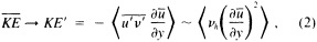
where we have assumed zonal symmetry and a zonal mean flow for simplicity. KE is kinetic energy, the overbar and prime denote mean and eddy components, and the angle brackets denote a volume average. The approximate magnitude of the associated horizontal eddy viscosity is vh ~ 104 m2 s–1, and the expected energy conversion is a significant fraction of the work done by the surface wind stress.
-
Mesoscale eddies effect the downward penetration of the wind-driven circulation and control its baroclinic structure. The downward penetration is as if there were a vertical stress of order vvV/H ~ 104 m2 s–1 (i.e., the order of the surface wind stress), which requires vv ~ 1 m2 s–1 for V ~ 0.1 m s–1 and H ~ 1 km characteristic of the gyre-scale circulations; yet it is clear from observations that vertical Reynolds stresses,
 and
and  , are many orders smaller than this requirement (see, e.g., Gregg, 1987). The mesoscale process that effects this penetration is isopycnal form stress: we define an internal stress
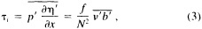
where p is the pressure and η is the elevation of an isopycnal surface. Thus, τi is an integrated form stress over an isopycnal surface; its vertical divergence then is a horizontal acceleration (here in the zonal direction). The second expression in (3) arises from the small-amplitude form of the definition of η (η = –b/N2, where b is the buoyancy field - gρ/ρ0 and N2 is the vertical gradient of b) and geostrophic balance
 . It also is associated with an exchange of energy between the mean and the eddies through buoyancy work,
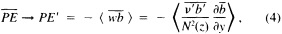
that is also of the same order as the wind work. Here PE is potential energy, and we have made use of the quasigeostrophic approximation and again assumed zonal symmetry. It is easy to see that substitution of a Fickian form for buoyancy flux implies energy losses from the mean fields.
-
Mesoscale eddies stir and make inevitable the mixing of both passive and dynamically active tracers, primarily along isopycnal surfaces (Iselin, 1939; Montgomery, 1940).
Dispersal statistics of neutrally buoyant floats in the ocean indicate that there is an effective diffusivity κi ~ 104 m2 s−1, but again with appreciable geographical variability (McWilliams et al., 1983). κi can also be related to isopycnal form stress (see below). There is the interesting possibility that these transports may often occur primarily in long-lived coherent vortices, and thus be highly non-local in that little "mixing" need occur over the long distances separating the generation and destruction sites (McWilliams, 1985).
At present the common practice in eddyless ocean models is to achieve (1) with a constant vh and to partially achieve (2) and (3) with a constant, and usually somewhat smaller, horizontal eddy diffusivity κh. The latter is formally equivalent to a κi at leading order in Rossby number (Ro = V/fL); however, it is clear that substantial differences in the tracer distributions result from κh versus κi, since the former implies substantial and excessive diapycnal fluxes across sloping isopycnal surfaces.
We have developed a novel parameterization scheme for the latter of these two roles, isopycnal form stress and isopycnal tracer diffusion (Gent and McWilliams, 1990; McWilliams and Gent, 1994). (The first role, horizontal momentum diffusion, seems less problematic in some ways, but it also needs to be extended beyond the present common practice of spatially constant viscosity.) The parameterization is chosen to have the following properties, which we collectively dub "quasi-adiabatic"; their rationale is that we want the quasi-adiabatic eddyless solutions to correspond to the large-scale components of an adiabatic, eddy-resolving solution.
-
All domain-averaged moments of potential density ρ are conserved, as is the volume between any two isopycnals.
-
With insulating boundary conditions, the domain average of any advectively conserved tracer S is conserved between any two isopycnals, and higher moments of S decrease in time if S has any gradients on the isopycnal surfaces.
-
The equation for a tracer S is satisfied identically by ρ.
Its mathematical form is as follows. In isopycnal coordinates, the equation for the thickness gradient ![]() is a combination of mass conservation (continuity) and the internal energy equation, viz.,
is a combination of mass conservation (continuity) and the internal energy equation, viz.,
where F is the isopycnal thickness flux by eddies that is the quantity to be parameterized. (Overbars are implied for all the fields in this section, and all vectors are only horizontal.) Equivalently, in either an isopycnal or physical-height coordinate frame, the associated internal-energy equation is
where Q is determined by
For any advectively conserved tracer S, the equation is
where D represents diffusion on an isopycnal surface with diffusivity κi
A particularly simple (and almost Fickian) choice for F and Q is
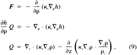
where the final expression is in physical-height coordinates. For κi > 0, any coordinate or resolved-flow-field dependence that respects the insulating boundary conditions and still satisfies the quasi-adiabatic constraints is acceptable. Furthermore, κi generally provides a down-gradient vertical flux of momentum (as an isopycnal form stress) and a loss of resolved-flow potential energy (as a baroclinic instability). We note that this form with D ≠ 0 and F = Q = 0 has previously been proposed (Redi, 1982) and implemented (Cox, 1987), but it has been found to be unsatisfactory in eddyless solutions because it cannot accomplish the necessary second role (above) for mesoscale transports, since F·∇ρρ = D [ρ] = 0.
This parameterization is an appropriate component of a balanced or primitive equation model of the general circulation, since it respects the finite-Ro deformations of isopycnal surfaces.
We have obtained eddyless solutions to equations (5) through (9) in the linear balance equations for a linear, single-component equation of state, ρ ∝ T, and a steady surface-wind stress that symmetrically forces a double gyre pattern. In these solutions the basin is a 4000 × 5000 × 5 km rectangular volume, and the gravest deformation radius is 45 km. Several results from these solutions are shown in Figures 1 through 4. A qualitatively sensible steady circulation results from the new parameterization with a spatially
constant ?i in combination with an also constant vh. It exhibits the broad pattern of the wind driving only in the upper ocean, but has cells of enhanced recirculation near the western boundary at all depths (Figure 1). The isopycnal mixing induces mean meridional-circulation cells (Figure 2) and an energy cycle in which eddy generation is mimicked as diffusive dissipation (Figure 3; note that these parameterized
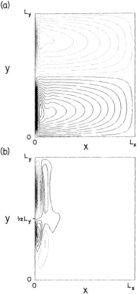
FIGURE 1
Horizontal stream function ?(x,y) at (a) upper-pycnocline and (b) deep-vertical levels in steady state for the wind-driven circulation with an isopycnal mixing parameterization in a linear balance-equation model. The wind pattern is symmetric about the middle latitude (y = Ly/2), with an eastward extremum there and equal westward extrema at y = 0 and y = Ly. The contour intervals are 0.1 and 0.005, respectively, in non-dimensional units.
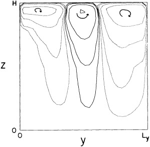
FIGURE 2
The mean meridional stream function ?(y,z) for the zonally averaged circulation for the same solution as in Figure 1. It is defined such that
The contours have a logarithmic distribution in unspecific nondimensional units.
eddy work terms are comparable to the mean wind work). However, these solutions are sensitive to spatial dependence in ?i, in ways that can influence, for example, the separation structure of the mean Gulf Stream (Figure 4). A more complete report is in McWilliams and Gent (1994).
Obviously there is a need to go beyond constant diffusivities if the eddyless solutions are to have the same large-scale circulations as those in equivalently forced eddy-resolving solutions. We currently are in the process of fitting plausible functional forms for vh and ?i to the eddy-flux patterns of eddy-resolving solutions for the wind-driven circulation. In particular we wish to examine the hypothesis that vhand ?i are often linked so as to make the down-gradient flux of potential vorticity the common situation (see, e.g., McWilliams and Chow, 1981; Marshall, 1981; Rhines and Young, 1982).
In Figures 5 through 8 are some preliminary results from this study. Notice that here the time-mean stream function has about the same peak amplitude near the western boundary in the middle of the gyres as in the analogous eddyless solution (Figure 1). Thus, the parameterization of equations (5) through (9) with a spatially constant diffusivity is working as it should, in some overall sense, in effecting the downward penetration of the wind-driven circulation; however, clearly it is not correct in matching the detailed patterns
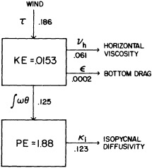
FIGURE 3
The energy budget in steady state for the same solution as in Figure 1. also in unspecified non-dimensional units.
of circulation. When we examine the patterns of the mean fields and their associated eddy fluxes (Figures 6 and 7), we see that both are structurally fairly smooth and simple. However, this does not necessarily imply that they will satisfy a Fickian relationship with equally simple patterns of eddy diffusivity. Figure 8 shows some examples of "minimal" eddy diffusivities, which are defined, e.g., for the horizontal diffusion of vorticity, to be
The sense in which this is minimal is that it is a solution of the more general relation
for which the scalar field E(ζ) contributes nothing to the eddy fluxes parallel to ![]() . Thus, (11) is an extension of the strictly Fickian relation (1). Note that any choice for E(ζ) provides an equivalent effect on the large-scale circulation when the divergence of the left side is taken, and any determination of v simply from knowledge of the mean field and eddy fluxes is inherently non-unique. However, rather than simply determining the eddy diffusivity as a spatial function that satisfies (11) for a particular solution, our goal should be to fit eddy diffusivities with dynamically plausible functional dependences on the large-scale flow fields, with the hope that these functional relations may turn out to be more general. In doing so, we can simultaneously avail ourselves of the arbitrariness of E in order to discover the best functional forms. Thus, in Figure 8 one can be struck with the structural complexity of the minimal eddy diffusivities, including their extensive regions of negative values (which are likely to be computationally ill
. Thus, (11) is an extension of the strictly Fickian relation (1). Note that any choice for E(ζ) provides an equivalent effect on the large-scale circulation when the divergence of the left side is taken, and any determination of v simply from knowledge of the mean field and eddy fluxes is inherently non-unique. However, rather than simply determining the eddy diffusivity as a spatial function that satisfies (11) for a particular solution, our goal should be to fit eddy diffusivities with dynamically plausible functional dependences on the large-scale flow fields, with the hope that these functional relations may turn out to be more general. In doing so, we can simultaneously avail ourselves of the arbitrariness of E in order to discover the best functional forms. Thus, in Figure 8 one can be struck with the structural complexity of the minimal eddy diffusivities, including their extensive regions of negative values (which are likely to be computationally ill
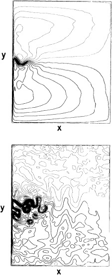
FIGURE 5
Time-mean and instantaneous ψ(x,y) in the upper pycnocline in an eddy-resolving, balance-equation variant of the problem defined in Figure 1. The contour interval is 0.2 in the same non-dimensional units.
behaved in a diffusion operator). Once the functional fitting has been made, however, the final diffusivity patterns may be quite different from those in Figure 8.
PLANETARY BOUNDARY LAYERS
The planetary boundary layers are usually the sites of the most intense three-dimensional turbulence in the oceans. Their spatial scales are bounded from above by the boundary layer depth (i.e., 10 to 103 m). Typical adjustment times for the PBL range from an eddy turnover time (~ 102 to 103 s) to an inertial time (~ 1/f = 104 s); both are short compared to the climatic times of interest.
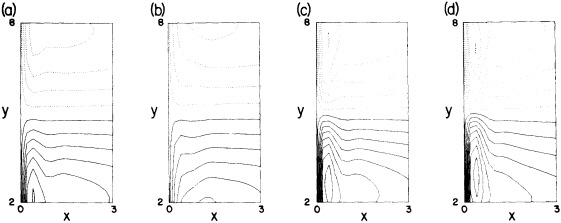
FIGURE 4
Upper-layer ψ(x,y) in the region of western-boundary current separation (i.e., 0 ≤ x ≤ 1500 km and 1000 ≤ y ≤ 4000 km) for different spatial/functional dependences of κi. Panel (a) is for the same solution as in Figure 1, which has a spatially uniform diffusivity; (b) has a linear dependence on the local kinetic energy density KE; (c) has the diffusivity vanishing in the western boundary current: and (d) has the combined features of (b) and (c). The contour interval is 0.2 in non-dimensional units.
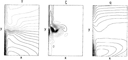
FIGURE 6
Time-mean and horizontally filtered temperature, vorticity, and potential-vorticity fields in arbitrary units in the middle pycnocline for the same solution as in Figure 5. Only a west-central 2000 km by 3000 km portion of the domain is displayed.
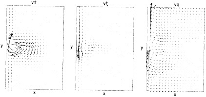
FIGURE 7
Filtered horizontal eddy fluxes of temperature, vorticity, and potential vorticity, in the same format as in Figure 6. Flux vectors have been deleted at the western boundary.
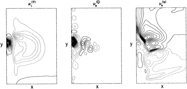
The PBL at the upper surface of the ocean provides an important reservoir for material properties being exchanged with the atmosphere, with a sequestration time of not more than a year. It also serves as a conduit transmitting atmospheric surface forcing to the interior, both for momentum (i.e., the Ekman velocity at the interior edge of the PBL) and material properties (often referred to as ventilation or subduction), which can lead to very much longer sequestration times. The transmissivity is much more efficient and inexorable for momentum than for the material properties; nevertheless, ventilation provides the principal sources and sinks for the interior, primarily isopycnal, tracer transports by mesoscale eddies (see above). The PBL at the bottom of the ocean provides a drag force on the adjacent currents, and, where there is an intersection with an isopycnal surface, as is particularly likely for a sloping bottom, it mixes material properties with locally diapycnal fluxes due to the three-dimensional motions in the PBL (Armi, 1978; Garrett, 1991; McCready and Rhines, 1991).
Present common practice in large-scale ocean models is to use linear Ekman relations at the top and bottom to transmit the boundary stresses to the interior motions, although in some instances a quadratic bottom-drag law is substituted, heuristically rationalized by analogy with non-rotating wall-bounded shear layers. Often the material-property transports are effected simply by extending the interior vertical diffusivities (see below) to the bounding surface. Insofar as these diffusivities are usually made large under conditions of static instability (or infinite, in an instantaneous adjustment to neutral stability), to some extent this procedure does mimic the PBL in at least this regime of penetrative vertical convection. Typically the vertical grid resolution near the upper boundary is taken to be so coarse (i.e., 50-100 m) that very little of the near-surface variability (e.g., the seasonal cycle) can be represented.
Nevertheless, it is something of a scientific oddity that, although many different types of PBL parameterizations have been proposed by meteorologists and oceanographers, they have seldom been used in atmospheric and oceanic general circulation models. If there is a conventional wisdom for what ought to be used in ocean models, probably it would be either a mixed-layer model (as in Garwood, 1977; Gaspar, 1988) or a second-order moment-closure model (as in Mellor and Yamada, 1982).
We have recently begun using yet a different type of PBL model that assumes neither that the mean profiles are vertically well-mixed—which they often are not—nor that the turbulent transports are wholly locally determined at any given vertical level—which clearly is incorrect, for example, in convective situations where boundary-generated plumes often traverse the layer. Also, in contrast to many of the previous, regime-specific proposals, we believe our parameterization to be valid in a broad range of conditions for the surface-buoyancy and -momentum fluxes and the mean profiles. Its essential basis is the hypothesis that the transport coefficients have a universal shape, but a vertical scale and amplitude that are particular to the local surface fluxes and mean profiles (O'Brien, 1970; Troen and Mahrt, 1986; Large et al., 1994).
We express the vertical turbulent fluxes of momentum, buoyancy, and passive scalars in the oceanic boundary layer in terms of a vertical diffusivity profile Kx(d), where x is any one of the above properties and d is the distance from the ocean surface. In certain circumstances a counter-gradient
profile γx(d) is also required. This term arises from an analysis of the turbulent temperature-variance budget (Deardorff, 1972; Holtslag and Moeng, 1991) and from observations in the atmosphere that show non-zero buoyancy fluxes where the local buoyancy gradient is zero or even weakly of the opposite sign (i.e., a local deviation from the Fickian form (1) is required to avoid large negative µ values). Throughout the boundary layer, h ≥ d ≥ 0, the fluxes are given by
The diffusivity profile is formulated to conform to known and desirable properties of boundary-layer turbulence. In the surface layer, ![]() (with
(with ![]() ), the semi-empirical results of Monin-Obukhov similarity theory should apply (Lumley and Panofsky, 1964). An important aspect of this is that the dimensionless flux profiles are universal functions,
), the semi-empirical results of Monin-Obukhov similarity theory should apply (Lumley and Panofsky, 1964). An important aspect of this is that the dimensionless flux profiles are universal functions, ![]() , of the stability coordinate ζ = d/L, where L is the Monin-Obukhov length scale,
, of the stability coordinate ζ = d/L, where L is the Monin-Obukhov length scale,
k is the von Karman constant, B0 is the surface buoyancy flux into the ocean, and (u*)2 is the kinematic surface wind stress. This leads to logarithmic mean-property profiles near the boundary; the associated fluxes are about 20 percent of their surface values at ![]() and approach their surface values linearly as d→0. Since there is no turbulent transfer either across the surface, or at d = h if the interior mixing is zero, the diffusivities must satisfy Kx(0) = Kx(h) = 0. The universal shape is assumed to be cubic in d, which has had rough empirical confirmation; thus,
and approach their surface values linearly as d→0. Since there is no turbulent transfer either across the surface, or at d = h if the interior mixing is zero, the diffusivities must satisfy Kx(0) = Kx(h) = 0. The universal shape is assumed to be cubic in d, which has had rough empirical confirmation; thus,
The turbulent velocity scale wx is formulated for consistency with similarity theory as a simple combination of the surface forcing velocities u* and w* (which is equal to (−B0h)1/3 if B0 is less than 0).
The counter-gradient term γx is non-zero only for the buoyancy field and for passive scalars in unstable forcing conditions (i.e., B0 < 0); thus, we restrict attention to x = s (for scalar). As suggested by Deardorff (1972), it has been successfully parameterized as
with Cs = 6.2.
The thickness of the oceanic planetary boundary layer h is determined as the smallest value of d at which a bulk Richardson number Rib across the boundary layer achieves a certain critical value Ric. Thus it primarily depends on the buoyancy profile b(d) and the velocity profile v(d), but there is also a (usually weak) dependence on the turbulent intensity:
The turbulent velocity vt combines with the mean velocity difference in the denominator of (14); its primary role is to establish the correct entrainment flux at the interior edge of the PBL when the mean velocity is weak or absent (i.e., primarily in the case of free convection). There is strong empirical evidence that this entrainment buoyancy flux ![]() is a fixed fraction, βT, of the surface buoyancy flux B0 = −
is a fixed fraction, βT, of the surface buoyancy flux B0 = − ![]() , viz., βT = 0.20 (see, e.g., Tennekes, 1973; this result is sometimes known as Turner's rule). With the parameterization forms above, it is achieved for
, viz., βT = 0.20 (see, e.g., Tennekes, 1973; this result is sometimes known as Turner's rule). With the parameterization forms above, it is achieved for
where ct = 5.8 is a constant that arises from the empirically determined stability function ![]() . Thus, from (16) and (17), h is larger, and hence the entrainment layer is thicker, where N(h) is smaller.
. Thus, from (16) and (17), h is larger, and hence the entrainment layer is thicker, where N(h) is smaller.
We have used this model, together with a new parameterization of internal vertical mixing described below that joins smoothly onto the PBL mixing at d = h, to calculate a variety of solutions, on time scales from hours to decades. Among these is one coupled to a one-dimensional radiative-convective atmosphere for the Ocean Weather Station Papa site in the North Pacific Ocean (Figures 9 through 11). The quality of its annual-cycle simulation is very good by the standards of previous upper-ocean PBL models (Martin, 1985), and we have found that an important part of this success is the inclusion of a diurnal cycle in insolation and an idealized, periodic storm cycle in the surface winds. To assess the consequences for climate modeling of accurately representing the oceanic annual cycle, we can compare Figure 11 with another coupled solution whose "ocean" is no more than a constant-depth mixed layer; it shows differences in tropospheric temperatures of up to 5 K in the annual cycle.
We are now in the process of extending and calibrating this new parameterization using large-eddy simulation solutions for the PBL under a variety of stress and buoyancy forcing conditions (e.g., Wyngaard and Moeng, 1993; McWilliams et al., 1993). We are particularly concerned with representing the asymmetry of scalar diffusivities forced by either surface or entrainment fluxes under convective conditions (Wyngaard and Brost, 1984). This effect is absent from the present parameterization forms, but it may be quite important for the diverse oceanic combinations of
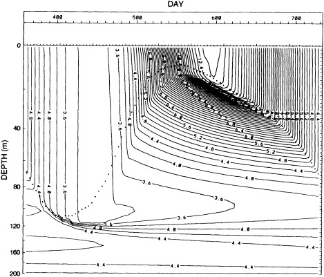
FIGURE 9
Four-day averages of oceanic T(z,t) in the upper North Pacific Ocean for a one-dimensional model using the PBL and interior vertical-mixing parameterizations of Large et al. (1994) and the radiative-convective atmosphere of Briegleb (1991), together with a specified surface wind consisting of the mean annual cycle (Trenberth et al., 1990) and an idealized "storm" cycle with a period of 4.1 days; the wind enters only in the bulk formulae for surface fluxes. Shown here is the second year of a two-year integration. The contour interval is 0.2 K. The dots indicate the base of the PBL, z = −h(t).
temperature and salinity stratification and surface forcing that occur.
INTERIOR VERTICAL MIXING
Under most circumstances, the vertical—more precisely, diapycnal—transports in the oceanic interior by small-scale motions are quite small. The associated eddy diffusivities are perhaps vv − 10−4 m2 s−1 and κv ~ 10−5 m2 s−1, and it is uncertain whether such small fluxes are important for climate variability on any except the longest time scales (millennia). However, under some circumstances these fluxes are locally very much larger and thus clearly of significance to the large-scale distributions of material properties.
The relevant small-scale processes are (1) shear and buoyancy (i.e., Kelvin-Helmholtz and convective) instabilities, which are regulated to some degree by the local, or gradient, Richardson number,
(2) double diffusive overturning motions, which are regulated by the ratio of temperature and salinity contributions to the density gradient,
and (3) internal wave breaking, which is regulated by properties such as wave steepness or proximity to a critical surface that are not expressible directly in terms of the large-scale wave environment. For this latter reason, we prefer to distinguish (1) and (3) in principle, although some proposals have been made that (3) should also depend on Rig (e.g., Gargett and Holloway, 1984).
There is clear evidence from observations (see, e.g., Peters et al., 1988) that vv and κv are greatly enhanced for small and negative values of Rig The extant measurements, however, have failed to collapse onto a universal curve, perhaps due to uncertainties in the determination of both the turbulent fluxes and the mean profiles. As yet this process has not been well modeled.
Conventional practice for parameterization of vertical
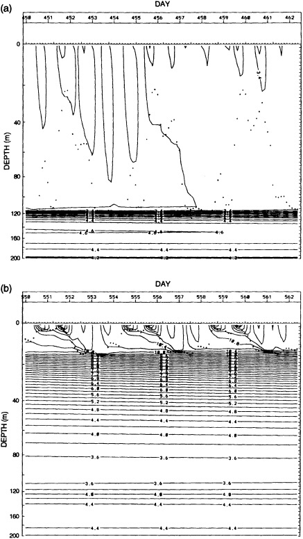
FIGURE 10
Instantaneous oceanic T(z,t) from the same solution as in Figure 9 for 12-day intervals in late winter (with contour interval of 0.1 K) and middle summer (with a contour interval of 0.2 K).
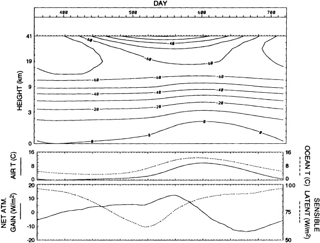
FIGURE 11
For the same solution as in Figure 9: atmospheric T(z,t) with contour interval 20.0 K; surface T(t) for the air (solid) and ocean (dashed); net atmospheric heat gain (solid) and net oceanic heat loss due to surface sensible and latent heat fluxes (dashed).
mixing is to use constant diffusivities with a large local enhancement in κv (and sometimes µv) where N2 is very small or negative, sometimes even one as extreme as an instantaneous convective adjustment. However, there has been increasingly widespread use of vv,κv[Rig] functions, usually of the form proposed by Pacanowski and Philander (1981), which has the qualitatively correct monotonic dependence on Rig, but is not particularly close to the observed values.
We have developed a variant formulation that explicitly includes all the processes enumerated above and matches the observations more closely, in spite of their uncertainties (Large et al., 1994). This parameterization is used in the solutions shown in Figures 9 through 11; we believe it contributes substantially to their quality, particularly during rapid oscillations in the PBL depth (as in Figure 10, e.g.) where the sub-PBL region often has smallish Rig values.
SGS TOPOGRAPHY AND MARGINAL ZONES
The necessary roles played by dynamical processes operating near bottom topography and in the coastal regions and marginal seas include the following:
-
Topographic Form Stress. Form stress can arise due to non-uniform pressure forces on the variable topography at the lower boundary in the ocean, just as it does on an airplane wing (or, as above, on a deformable isopycnal surface). The zonal form stress is defined, assuming geostrophy, by
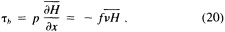
where H(x,y) is the variation of the bottom elevation about its mean. This stress enters into a mean zonal-momentum balance at the lowest level in an ocean model.
It seems clear that topographic stresses often are of sig-
-
nificance to the large-scale flow. This has been shown in idealized contexts by Bretherton and Haidvogel (1976), Holloway (1978, 1987), and Treguier (1989). It seems particularly relevant for the Antarctic Circumpolar Current (McWilliams et al., 1978; Treguier and McWilliams, 1990; Wolff et al., 1991), and it also is probably so for the continental slopes (Holloway, 1992). Unfortunately, it currently is not included as a SGS process in most large-scale ocean models.
-
Material Property Mixing. The boundary regions of the ocean, including the continental shelves and marginal seas, have especially high biological productivity, anomalous chemical sources because of river runoff and human pollution, and strong local mixing because of both strong tidal flows and shallow depths that permit the boundary layer to encompass the whole water column. These processes are not commonly part of the SGS parameterizations in large-scale ocean models.
-
Rapid Communication in the Boundary Wave Guide. The sides of ocean basins can support a rich variety of coastal waves (LeBlond and Mysak, 1978). In the simplest geometry, with vertical sides, these waves are Kelvin waves. They have an off-shore scale of the deformation radius (tens of km) and travel at the rapid speed of short gravity waves. They play an important dynamical role in communicating changes in the boundary-pressure distribution along the coastline and establishing along-shore currents of deformation-radius width. Since this scale lies in the SGS range for large-scale ocean models, there is a question of how to incorporate these effects adequately. Milliff and McWilliams (1994) have shown that the outcomes of these communication events by waves can at least sometimes be accurately represented by simple, integral consistency constraints on the large-scale fields.
SEA ICE
A sea-ice parameterization is a necessary element of an oceanic climate model. In its simplest, most often used form, it is merely a thermodynamic model for a temperature profile within a layer of ice of a certain thickness. The parameterization allows for storage of heat and water and alteration of the air-sea fluxes. Yet it is also important to model both sea ice's concentration, since the fraction of open water (or leads) makes an enormous difference to the air/sea heat and water fluxes, and its horizontal movements. Modeling the concentration and movements requires the inclusion of mechanical dynamics as well.
In our own modeling studies, we are following the formulation of Hibler (1979), in part as it has been extended by Lemke et al. (1990) and by Flato and Hibler (1990).
BIOGEOCHEMICAL PROCESSES
Oceanic biochemistry is a necessary element of any oceanic climate model that addresses either the oceanic distributions of nutrients, oxygen, and so on, or the global cycle for CO2, et al. I hesitate to declare a common current practice for ocean models, but guidance can be found in the recent study by Sarmiento et al. (1993).
Scott Doney, David Glover, and Raymond Najjar are developing a simple ecosystem model for the upper ocean that is based on the flow of nitrogen among organic and inorganic constituents. A solution for the annual cycle in the Sargasso Sea near Bermuda is shown in Figure 12. There are some attractive features: the timing of the spring phytoplankton bloom that follows the wintertime renewal of nutrients by deep PBL mixing and ends with their depletion in the well-mixed layer; the summertime subsurface maximum of phytoplankton that live on the border between nutrients in the seasonal pycnocline and penetrating solar radiation; and the somewhat deeper subsurface maximum in nutrients associated with the remineralization of sinking particles below the solar penetration.
ACKNOWLEDGMENTS
It seems increasingly clear to me that any serious climate modeling that goes beyond the initial conception of new possibilities requires the cooperation of many scientists. The scope and tasks are so large that pooled knowledge and labor seem nearly essential. In this spirit, I would like to thank my current partners in the work touched on in this paper: Bruce Briegleb, Gokhan Danabasoglu, Scott Doney, Peter Gent, Jeff Kiehl, Bill Large, Chin-Hoh Moeng, Jan Morzel, Ralph Milliff, Nancy Norton, Breck Owens, Mike Spall, Peter Sullivan, and John Wyngaard. In addition, I thank Kirk Bryan for his comments both during the workshop and in a review of this manuscript. The work is sponsored, under various contracts, by the National Science Foundation and the National Oceanic and Atmospheric Administration.
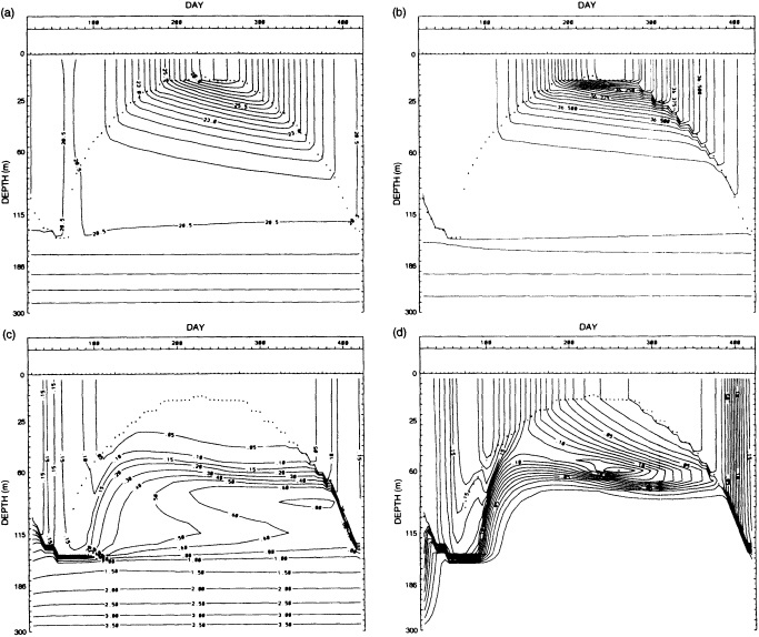
FIGURE 12
Depth and time dependence for (a) temperature [°C], (b) salinity [ ![]() ], (c) nutrients [mmol/m3 of equivalent nitrogen], and (d) phytoplankton [mmol/m3 of equivalent nitrogen] in a Sargasso Sea, annual-cycle solution with the physical dynamics of Large et al. (1994) and the ecosystem dynamics of Doney and Najjar. Again, the dots indicate the base of the PBL, where z = - h(t).
], (c) nutrients [mmol/m3 of equivalent nitrogen], and (d) phytoplankton [mmol/m3 of equivalent nitrogen] in a Sargasso Sea, annual-cycle solution with the physical dynamics of Large et al. (1994) and the ecosystem dynamics of Doney and Najjar. Again, the dots indicate the base of the PBL, where z = - h(t).
Commentary on the Paper of McWilliams
KIRK BRYAN
NOAA/Geophysical Fluid Dynamics Laboratory
In reading this paper, I felt that it is very good news indeed that our field has reached the point at which somebody with Dr. McWilliams's qualifications in geophysical fluid dynamics is taking climate seriously enough to devote his full attention to improving ocean models for climate.
I have a couple of questions: First, does it make sense to design a very general ocean climate model rather than one for each problem? Second, can we represent these climatically important features such as overflows and deep western boundary currents—and this has come up in conversations I have had here with Drs. Dickson and Lazier—without going down to eddy-resolving resolution? Even if we are not greatly interested in mesoscale eddies, the boundary currents require very high resolution. I am a little more optimistic than Dr. McWilliams; I think that with massively parallel computers we will be able to resolve longer time scales and shorter spatial scales somewhat sooner than his prediction of 10 or 20 years. Admittedly, trying to run global calculations to something like equilibrium is a very stiff requirement.
Let me just comment on some of the topics that this paper addresses. One item is the parameterization of thickness mixing. I feel that this is a very important contribution. Another is lateral boundaries. I am a little skeptical as to whether a 100-km resolution is going to be adequate. Third, the approach to the planetary boundary layer seems like a good one.
One other point that Claes Rooth brought up earlier is that convection is not mentioned in the paper. Convection is often pointed out as a major weakness of these models. Is that taken care of by thickness mixing and mixing along isopycnals?
Discussion
MCWILLIAMS: The rationale for focusing on the upper ocean, at least for a certain range of time scales as we develop and try out new parameterizations, is the following. At present we are confronted with very serious climate drifts that appear at early times in most coupled calculations, as indicated by the large-amplitude flux corrections that are commonly used to control the equilibrium state in such models. These drifts seem to be associated with near-interface processes, in that the air-sea fluxes of momentum and latent and sensible heat are controlled by the planetary boundary layers. The atmospheric boundary layer interacts strongly with the stratus and cumulus clouds that in turn strongly regulate the precipitation. Since full-depth ocean models are very expensive to use and have ill-defined quasi-equilibrium states except on very long time scales, I think it's useful to give an upper-ocean domain a climatological lower boundary condition in order to be able to efficiently calculate evolution on shorter time scales, from months to decades. The resulting model should be capable of calculating reasonably accurately the variability of large-scale material properties, like T and S, in the upper ocean. In this domain we could use fairly high vertical-grid resolution, make calculations reasonably cheaply, look at coupled solutions with the atmosphere and sea ice, and try to sort out some of the coupled dynamics, including the sources of spurious climate drift.
We are taking the GFDL model as our starting point, and putting it in a form in which we can put the sigma coordinate at the bottom so that it can be a full ocean model. As we look at shorter variability time scales we don't expect that to be our primary mode. While we're trying to deal with complex general circulation questions, we certainly don't want to spend our energies on a proliferation of models. But I do see an interim utility in trying to isolate upper-ocean interactions with climate.
MYSAK: Away from boundaries we can get away with an upper-ocean model. But if interannual and even decadal variabilities are perturbations in the seasonal cycle, for which topography is very important for many of the flows, then such models will not describe real climate variability at high latitudes.
MCWILLIAMS: My sense is that except for essentially barotropic currents, which are of limited importance here, there isn't much penetration to depth. I agree that in the northern high latitudes topographic complexity is a real problem, but the full ocean models can't deal with that either. I don't see it as a prime obstacle to progress in, say, global coupling issues.
CANE: I'd like to comment on the need for one grand model versus many smaller ones. I find that a complicated model tends to distract you from things that might require attention, such as the mixed layer. I don't think there's a way of doing it all.
Second, I'm not sure that eddy resolution is the most important issue. For instance, topography might be important for the deep-circulation modes. But at present, with a 100-km grid, we can't get the width of the Gulf Stream right. That means we can't get its speed and transport right either, which we need for some of
the air-sea interaction problems. There may be other approaches, aside from a full high-resolution model, we should be looking at.
MCWILLIAMS: Surface material-property distributions near the Gulf Stream tend to be a pretty broad envelope, since there are both advection by the narrow stream and buffeting by eddies. For climate you need to get the current's transport right, but not necessarily its narrowness and speed maximum.
CANE: I think you'd need to get the advective transport of warmer waters about right in order to get the fluxes right. I think it could be done without introducing tremendous resolution everywhere.
MCWILLIAMS: It's a burden on the sub-grid-scale parameterization. Progress will be made in both resolution and parameterizations, but I think we need to make what you might call the mesoscale calculations before we look at the details of, say, topography. Someone needs to examine topographic parameterization. In the end, of course, it might have to be done with local high-resolution grids for particularly complex regions.
BERGMAN: Is it possible to use variable grids to resolve features like the western boundary currents, yet still have a model that is not excessively complex overall?
BRYAN: Non-uniform grids are used extensively in engineering calculations. But you must then use a very implicit type of calculation, or the time step will be limited by the smallest grid size.
BERGMAN: Are semi-lagrangian approaches being tried for ocean GCMs as well as atmospheric GCMs?
MCWILLIAMS: Yes, some people are pursuing this idea; semi-lagrangian schemes that are sort of shape-preserving keep you from being embarrassed by things like negative concentrations. I myself feel that we can develop multi-grid, fully implicit problem-solvers that can be run at Courant-Friedrichs-Levy numbers of 10 or so, which is a considerable potential economy over semi-lagrangian schemes.
DICKSON: It seems to me that you need a comprehensive observing system to give you a long-period look at the ocean against which you could match a comprehensive climate model's results.
MCWILLIAMS: I quite agree. But please invite the modelers to join the design process!
A Stochastic Model of North Atlantic Climate Variability on Decade-to-Century Time Scales
KIRK BRYAN1 AND FRANK C. HANSEN2
ABSTRACT
A conceptual model of North Atlantic climate variability is based on a simple two-box representation of the thermohaline circulation of the ocean. The model is linearized about a basic state, which corresponds approximately to the present ocean climate of the North Atlantic. Stochastic forcing, which represents the random effects of atmospheric cyclones and anticyclones passing over the ocean surface, drives the model away from its equilibrium state. The model transforms this stochastic forcing with equal power at all frequencies into a red-noise response in ocean temperature and salinity. At frequencies less than the thermohaline circulation's time scale, the solution is an equilibrium response and the amplitude of model ocean climate becomes independent of frequency.
Damping of salinity variations in the model is due to the thermohaline circulation. Ocean temperature variations are damped by both the thermohaline circulation and interaction with the atmosphere at the ocean surface.
The model illustrates how air-sea interaction involving the thermohaline circulation could produce a continuous spectrum without peaks. Stochastic forcing amplitudes corresponding to the climate of the last few thousand years produce a nearly linear response of the model. Large perturbations of the hydrological cycle typical of the close of the last ice age produce a chaotic response.
INTRODUCTION
The instrumental climate record now extends over a century. Although the record contains many gaps in both space and time, it is still possible to find very-large-scale climate variations that extend over several decades (Folland et al., 1986). These fluctuations are quite distinct from the climate variations related to the El Nino* phenomenon. The El Nino fluctuations have a time scale of three to four years and tend to have their greatest amplitude in the equatorial Pacific. The El Nino climate variations are associated with changes in tropical atmospheric convection, and cause changes in air temperature extending up to the base of the
stratosphere. On the other hand, the very-low-frequency climate variations tend to be amplified in polar latitudes and have their greatest amplitude near the earth's surface.
The most unambiguous evidence for low-frequency climate variations with a period of several decades comes from surface temperature records over land. Figure 1 shows the historical temperature record averaged by latitude belts (Hansen and Lebedeff, 1987). Several features stand out in Figure 1. First, there is a clear upward trend in temperature over the past century, which is greatest in the higher latitudes of the Northern Hemisphere. Second, very-low-frequency
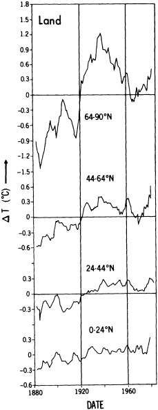
FIGURE 1
Zonally averaged surface temperatures over land, compiled by Hansen and Lebedeff (1987). Note the low-frequency variability superimposed on the upward trend over the past century.
variations are superimposed on that trend. The most obvious features are pronounced minima at the beginning of the century and in the late 1960s and early 1970s. In between these two relatively cold events there was a period of relatively rapid warming in the 1920s. The most recent part of the record is not shown in Figure 1, but measurements indicate that Northern Hemisphere temperatures are rising rapidly in the 1980s, as they did in the 1920s (IPCC, 1990).
Bjerknes (1964) studied the pre-World War II climatic record, particularly the sea surface temperature archives of the British Meteorological Office. He was impressed by the relatively rapid rise of Northern Hemisphere temperature in the 1920s, which followed an anomalously cold period at the beginning of the century. In his analysis of the sea surface temperature and the surface atmospheric pressure fields at mid-latitudes he found a distinct difference between the fluctuations that had a time scale of seasons and years and the climatic fluctuations, which were on decadal time scales. Bjerknes concluded that the atmosphere played the dominant role in those fluctuations with a yearly time scale, while the ocean played the dominant role in the climatic fluctuations. He was aware of the heat-balance calculations carried out by Sverdrup (1957) and realized that the North Atlantic is much more important than the North Pacific in the poleward transport of heat in higher latitudes. He reasoned that fluctuations in the North Atlantic poleward heat transport could be the cause of decadal-scale Northern Hemisphere climate variations. Bjerknes' hypothesis received relatively little attention in 1964. Since so little was known about ocean circulation at the time, his ideas probably seemed to be difficult to check in any way. On the other hand, his explanation of the onset of the Southern Oscillation (Bjerknes, 1969) in terms of the Walker circulation was widely accepted within a few years after publication.
A few years previous to the publication of Bjerknes' study of the Atlantic, Stommel (1961) developed a simple model of the thermohaline circulation. He pointed out that air-sea interaction has a very different effect on the temperature field of the ocean than on the salinity field. The radiation balance of the atmosphere directly responds to the sea surface temperature field, while a similar feedback cannot exist for salinity. When this asymmetry was taken into account, Stommel demonstrated, his simple model of the thermohaline circulation could take on two stable solutions for the same external boundary conditions. In one solution the thermohaline solution was dominated by the thermal component of the density gradient, and in the other solution the salinity component of the density gradient was most important. In recent years it has been possible to test the concepts of Stommel's two-box thermohaline model in more complete two- and three-dimensional models (see Weaver and Hughes, 1992, for a review). Through these recent numerical
studies the fundamental importance of Stommel's 1961 paper has become more widely recognized.
Hasselmann (1976) demonstrated in a simple way how the heat-storage capacity of the upper ocean acts to integrate random heat impulses from the atmosphere. This integrating property of the upper ocean greatly amplifies the response of sea surface temperature to low-frequency heating inputs. In Hasselmann's stochastic model the excursions of sea surface temperature about equilibrium are taken to be the result of a random-walk process, which is limited in amplitude by atmospheric feedback. In Hasselmann's model, air-sea interaction is purely local within the ocean. However, this elegantly simple model runs into difficulties when an attempt is made to generalize it to include salinity as well as temperature. For a random-walk process on the temperature-salinity plane driven by stochastic forcing there is no physically plausible mechanism to limit extreme anomalies of vertically averaged salinity, as there is for temperature. This difficulty is removed only by allowing for a nonlocal process that permits exchange with other parts of the world ocean. A stable regime in Stommel's two-box model of the thermohaline circulation driven by stochastic forcing represents the simplest extension of Hasselmann's ocean climate model, which can include salinity as well as temperature.
The motivation for attempting to construct a simple toy model of this kind is the success of much more complex numerical models that illustrate oscillations of thermohaline circulation. Examples are studies by Weaver and Sarachik (1991b), Mikolajewicz and Maier-Reimer (1990), and Delworth et al. (1995, in this volume). The calculations by Mikolajewicz and Maier-Reimer were carried out for a numerical model of the world ocean. Surface temperature is damped toward observed values, but stochastic forcing is used to simulate observed variations of the net water flux at the surface. It was found that stable oscillations of the Atlantic thermohaline circulation took place with a maximum amplitude at a period of several centuries. Delworth et al. studied a fully coupled ocean-atmosphere model. Their results illustrate climate fluctuations consistent with Bjerknes' (1964) hypothesis for Atlantic climate variability. Variations in the strength of the thermohaline circulation are correlated with decadal-scale sea surface temperature anomalies that seem to be quite realistic when compared with analyses of the Comprehensive Ocean-Atmosphere Data Set (COADS) by Kushnir (1994). The aim of the present study is to construct a simpler framework for understanding the important results of these physically complete but highly complex models.
HASSELMANN'S MODEL
Since Hasselmann's (1976) stochastic model of climate is an important point of departure for the present study, we will review it briefly. Consider a reservoir of upper ocean water as shown in Figure 2a. Let T' be the departure of the temperature from its climatological average. The governing equation is
where D is the depth of the reservoir, and Q is the average temperature change in the reservoir due to heating, which is associated with the random fluctuations of cyclones and anticyclones at the ocean surface. Temperature fluctuations are damped by the term, − λT'/D, on the right-hand side of (1). This negative feedback term represents the combined effects of long-wave radiation, evaporative cooling, and sensible heating, all of which are closely related to ocean surface temperature. Let
Hasselmann (1976) assumes that the effect of ''weather" over the ocean can be represented as white noise, where |Qw| is thus uniform at all frequencies. The power spectrum of the solution of (1) may be written as
The spectrum given by (3) has two very different regimes. In the high-frequency regime, where ω ![]() λ/D, "white noise" forcing gives rise to a "red noise" response. This can be understood physically as the effect of the memory of the ocean. Hasselmann (1976) describes it as a random-walk process in one dimension. Excursions from the origin become longer and longer over greater and greater time scales.
λ/D, "white noise" forcing gives rise to a "red noise" response. This can be understood physically as the effect of the memory of the ocean. Hasselmann (1976) describes it as a random-walk process in one dimension. Excursions from the origin become longer and longer over greater and greater time scales.
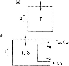
FIGURE 2
(a) A schematic diagram of Hasselmann's (1976) stochastic climate model. (b) A generalized model, such as that of Stommel (1961), that includes salinity and communication to other regions of the ocean.
The negative-feedback term provides a restraint to the random-walk process at very low frequencies, ω ![]() λ/D. At this point, |Tω| becomes simply proportional to |Qω|, which has a uniform value at all frequencies. In this second regime, forcing and negative feedback are in exact balance. We will designate this low-frequency part of the spectrum as an equilibrium response regime.
λ/D. At this point, |Tω| becomes simply proportional to |Qω|, which has a uniform value at all frequencies. In this second regime, forcing and negative feedback are in exact balance. We will designate this low-frequency part of the spectrum as an equilibrium response regime.
THE EFFECTS OF SALINITY
Suppose we consider a more general case, in which the same reservoir model has departures of both temperature and salinity from equilibrium. Random variations of excess evaporation over precipitation will be associated with the same weather events responsible for stochastic heating in the original Hasselmann model. Instead of a one-dimensional random-walk process, we can think of a two-dimensional random walk in the T−S plane. A true random walk is physically unlikely, because heating and evaporation minus precipitation tend to be negatively correlated.
There is one insurmountable difficulty to a purely local model of this type. No feedback mechanism can be invoked that will damp excursions in salinity in the same way that temperature excursions are damped by interaction with the atmosphere. A random walk process on the T−S plane would thus be limited in the T-direction, but could attain extreme states of very high or very low salinity. The Great Salt Lake and the Great Lakes are examples of isolated water bodies with extremely high and low salinity values, respectively. Thus we are forced to abandon the elegantly simple model of Hasselmann and include nonlocal effects. Figure 2b shows how a one-box model can be generalized to include communication with the world ocean, thus avoiding an infrared catastrophe in salinity.
STOMMEL'S MODEL
Fortunately, the equations governing the nonlocal model shown in Figure 2b are almost the same as those for Stommel's (1961) classical two-box model of the thermohaline circulation. Stommel's model has recently been revisited by Huang et al. (1992). More complex versions of the model have also been investigated by Marotzke (1990) and Birchfield et al. (1990). The most important result of Stommel's (1961) original study was the demonstration that the thermohaline circulation can have multiple equilibrium states in response to only small changes in surface forcing. This fundamental idea has been the basis for many recent studies with much more elaborate models (Bryan, 1986b; Manabe and Stouffer, 1988).
Let V and D be the volume and depth of the reservoir, which represents the subarctic gyre of the North Atlantic. Let T and S be the average temperature and salinity of the subarctic gyre, while Tω and Sω are the fixed temperature and salinity of the rest of the World Ocean. Let
where T* is a fixed reference temperature for the subarctic box. The equations for T and S are then
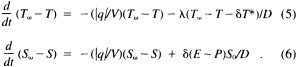
Here q is the exchange of water between the subarctic gyre and the remainder of the ocean, as indicated in Figure 2. The effect of the first term on the right-hand side of both (5) and (6) is to diminish the contrast between the world ocean and the subarctic box. A key time scale of the problem is given by V/q. For the present circulation of the North Atlantic, this overturning time scale is about 25 years. The second term on the right-hand side of (5) is the heating term, which forces the temperature of the subarctic box to depart from Tω, the temperature of the world ocean. Air-sea interaction forces T toward the reference value of Tω − δT* on a damping time scale given by D/λ. The second term on the right-hand side of (6) represents the effect of north-south contrasts in evaporation and precipitation that force the salinity of the subarctic box to depart from the salinity of the world ocean. Note that (5) includes a feedback due to air-sea interaction, while (6) has no corresponding term. In our toy model, the forcing terms on the right-hand side of (5) and (6) will have both a steady component and a stochastic component.
Stommel (1961) specified that the transport, q, of the thermohaline circulation should be proportional to the density difference between the reservoirs, such that
where α and β are expansion coefficients for temperature and salinity, respectively, and µ is a constant of proportionality relating transport to the density difference. For the North Atlantic thermohaline circulation, an appropriate value of µ would be approximately 10 sverdrups (107 m3 s−1) per sigma unit of density (kg m−3) (Roemmich and Wunsch, 1985).
To gain some insight on the sensitivity of the model to specified parameters, a rescaling is useful. Let ![]() be the time-averaged value of δT*; then
be the time-averaged value of δT*; then
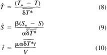
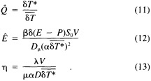
Huang et al. (1992) chose to scale the Stommel 2 × 1 box model by the damping time scale, D/λ. We have chosen to use the circulation time scale, V/q. This introduces a significant simplification, which we will point out later. It also has the advantage that the circulation time scale can be estimated from measurements of overturning at 24°N (Roemmich and Wunsch, 1985), while the damping time scale due to air-sea interaction is more difficult to estimate. Temperature is scaled by the difference between the reference temperatures of the subarctic box and the world ocean. The density difference due to salinity is scaled by the density difference associated with ![]() .
. ![]() is defined so that it is unity plus a stochastic component that averages to zero with respect to time. Ê is scaled by the circulation time and a factor to remove the salinity dimension. η is the circulation time scale divided by the atmospheric thermal damping time scale. An appropriate value for this parameter is discussed below. Substituting equations (7)−(13) into (4)−(6), we obtain
is defined so that it is unity plus a stochastic component that averages to zero with respect to time. Ê is scaled by the circulation time and a factor to remove the salinity dimension. η is the circulation time scale divided by the atmospheric thermal damping time scale. An appropriate value for this parameter is discussed below. Substituting equations (7)−(13) into (4)−(6), we obtain
Steady-state solutions of a model very much like (14) and (15) were originally explored by Stommel (1961). He found a maximum of three possible steady-state solutions. In one of these solutions, ![]() is greater than
is greater than ![]() , indicating that the density gradient between the boxes is dominated by temperature. Stommel identified this solution with present climate. Another stable solution existed for
, indicating that the density gradient between the boxes is dominated by temperature. Stommel identified this solution with present climate. Another stable solution existed for ![]() greater than
greater than ![]() , which corresponds to the case of a reversed and weak thermohaline solution dominated by salinity. These solutions are also discussed in detail by Huang et al. (1992), who also explore more elaborate models that include several degrees of freedom in the vertical direction. Eq. (15) is the non-diffusive form of a model described by Spall (1992), although, unlike our model, Spall's includes a mixed layer.
, which corresponds to the case of a reversed and weak thermohaline solution dominated by salinity. These solutions are also discussed in detail by Huang et al. (1992), who also explore more elaborate models that include several degrees of freedom in the vertical direction. Eq. (15) is the non-diffusive form of a model described by Spall (1992), although, unlike our model, Spall's includes a mixed layer.
In (14) and (15), the derivatives on the left-hand side are taken with respect to nondimensional time. For convenience, the steady-state values of ![]() and
and ![]() will henceforth be referred to as T and S.
will henceforth be referred to as T and S.
STEADY SOLUTIONS CORRESPONDING TO NORTH ATLANTIC CLIMATE
The motivation for this study is the question of whether small oscillations of the thermohaline circulation could be responsible for decadal climate variations over the North Atlantic, as was proposed by Bjerknes (1964). For this reason, we wish to make a detailed study of a linearized version of Stommel's model in the vicinity of a steady-state solution that approximates the present circulation of the North Atlantic. It is important for this purpose to examine the physical interpretation and plausible range of the model parameters. Table 1, in which V corresponds to the volume of the Atlantic from the surface to the bottom between 52° and 75°N, presents their values. We see from Table 1 that the basic time scale is about a few decades for a thermohaline circulation of 13.3 × 10⁶ m3 s−1 and a volume corresponding to the subarctic gyre of the North Atlantic. A plausible damping time scale is more difficult to estimate. Using a value of λ given by Haney (1971), we get a damping time scale of only a decade. Using a smaller value of λ more appropriate for a large geographical area and a depth on the order of the basin depth (Schopf, 1985), we obtain a damping time scale of nearly a century. Corresponding values of η range from 0.25 to 2.5. The depth over which feedback to the air is relevant for fluctuations on a decade-to-century time scale is the depth of the basin. The fact that the time scales of thermal damping and of the thermohaline circulation are nearly the same is a key feature of the physics of our model.
If we consider the steady-state version of (14) and (15), the curves corresponding to (14) are those shown as solid lines in Figure 3. The curves corresponding to (15) are those shown as dashed lines. The manifold of solid curves corresponds to different values of the damping coefficient η. The different dashed lines correspond to different values of the salinity forcing parameter, E. Solutions correspond to intersection points of these two curves. Note that at most two intersection points exist for T > S, which corresponds to the present state of the North Atlantic, where the thermal component of the density gradient dominates the salinity component.
The thermal equation (14) gives a family of nearly straight lines for different values of η. As η increases, the lines become more nearly horizontal and are asymptotic to T = 1 as η goes to infinity. On the other hand, the salinity
TABLE 1 Plausible Values of Model Parameters
|
Parameter |
Symbol |
Value |
|
Depth |
D |
4 × 10³ m |
|
Volume |
V |
1 × 10¹⁶ m3 |
|
Transport |
|
1.33 × 10⁷ m3 s−1 |
|
Feedback Parameter |
λ |
0.133 − 1.33 × 10⁻⁵ m s−1 |
|
Circulation Time Scale |
|
7.5 × 10⁸ sec (≈24 yr) |
|
Damping Time Scale |
D/λ |
0.3 − 3.0 × 10⁹ sec |
|
Damping Coefficient |
0.25 − 2.5 |
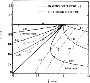
FIGURE 3
Steady-state solutions of the model are given by the intersection points of the solid lines (bold-faced numbers), which correspond to the different values of the damping parameter, and the dashed lines (italic numbers), which correspond to different values of E, the nondimensional evaporation-minus-precipitation forcing. The diagonal line separates the thermal regime, in which temperature differences dominate the poleward density gradients, from the haline, in which salinity dominates.
equation (15) gives a family of curves that penetrate further below T = 1 for weaker haline forcing.
STOCHASTIC FORCING OF THE THERMALLY DOMINATED REGIME
In this section we will consider the results obtained by stochastic forcing of a version of the Stommel model with no restoring of the salinity field. The stability of the Stommel two-box model has been discussed by previous authors (Huang et al., 1992; Marotzke, 1990; Stommel, 1961; Walin, 1985). The results of the linear analysis of our model are shown in Figure 4. Damped harmonic solutions exist for T < S < T/(2T − 1)2. Unstable real roots exist in the region bounded by S = T(2 − T)/2 and T = S. The remaining areas have simple damped solutions. In the North Atlantic, geologic evidence suggests that a thermally dominated thermohaline regime has existed since the close of the last ice age, 10,000 years ago. Therefore, it appears that the stable regime in which S < T(2 − T)/2 in our model corresponds to the present climate of the North Atlantic. The remainder of this paper is concerned with the analysis of the response to forced oscillation about the stable equilibrium in the thermally dominated regime of the model.
To check our calculations we calculated the linear response analytically and compared it to the results of direct
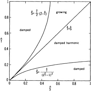
FIGURE 4
A map of the T-S plane showing the results of a linear-stability analysis of steady-state solutions of the model. Unstable solutions are only found in the region T(2 − T)/2 < S < T. In the remaining regions, solutions are either simply damped or harmonically damped.
numerical integration of the full nonlinear model with very small stochastic forcing. It is appealing to think of the effect of air-sea fluxes associated with cyclones and anticyclones passing over the ocean as causing a random walk in vertically integrated water-mass properties. Results from the GFDL coupled model show that heating and net evaporation-minus-precipitation at the ocean surface are negatively correlated. The results of Delworth et al. (1995) show that surface fluxes tend to heat and simultaneously freshen the ocean surface or, conversely, cool the ocean surface and make it more saline. Rather than making heating and evaporation-minus-precipitation independent random variables, we made them proportional to one another, with opposite sign, in our stochastic model.
Analytic spectra for the three cases are shown in Figure 5. Figure 5a corresponds to the case in which η = 2 and the steady component of E = 0.1. Q' is 10 times larger than E' and of opposite sign, causing the temperature fluctuations to be larger than the salinity fluctuations at all frequencies. At high frequencies, both spectra have a slope of ω–2. Damping becomes important for salinity only at frequencies less than 0.1 cycles/unit time, which corresponds to a period of 240 years. Figure 5b shows a case that is the same as that of Figure 5a, except that ηQ' is now twice −E'. |T2| is exactly four times longer than |S2| at high frequencies, but a crossover point is reached at a period between 50 and 100 years. The effect of removing the thermohaline coupling term is shown in Figure 5c. This case corresponds to the
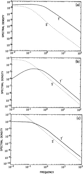
FIGURE 5
The spectral density of density variations due to temperature (solid line) and salinity (dashed line) as a function of frequency in cycles per unit of nondimensional time. Eta, the thermal damping parameter, is equal to 2, and the steady state component of E equals 0.1. (a) Random heating is 10 times the salinity forcing. (b) The same as (a), but the heating is equal to the salinity forcing. (c) The same as (b), but the thermohaline circulation is eliminated, corresponding to the Hasselmann (1976) model.
Hasselmann (1976) model. Temperature is damped by interaction with the atmosphere, but salinity increases without bounds as frequency decreases. This is the infrared catastrophe for salinity noted earlier.
The phase relations predicted by the model are shown in Table 2 for periods corresponding to 48, 96, and 240 years, assuming that one unit of nondimensional time is equivalent to 24 years. Amplitude and phase relationships are for E = 0.1 and η = 2.0, and different ratios of E' to Q'. θT is the phase of T with respect to the thermohaline circulation. θ−S is the phase of −S with respect to the thermohaline circulation. (A) corresponds to a clockwise orbit on the T−S plane, while (B) and (C) correspond to counterclockwise orbits. Of particular interest are the phase relationships between the density anomalies, which are a function of temperature and salinity, in both the subarctic gyre and the thermohaline circulation. Delworth et al. (1995) find that in their three-dimensional coupled model, density anomalies due to temperature lead the thermohaline circulation, and density anomalies due to salinity tend to lag slightly. Since ![]() is proportional to Tω − T, it is also proportional to the thermal density component in the polar box. On the other hand, the haline density component is proportional to −S.
is proportional to Tω − T, it is also proportional to the thermal density component in the polar box. On the other hand, the haline density component is proportional to −S.
The first entry in the table corresponds to a positive correlation between E' and Q' perturbations, which have equal magnitude. The model shows that the response in temperature and salinity are nearly equal, and the − S component leads the thermohaline circulation, while the T component lags behind. Delworth et al. (1995) find just the opposite phase relationship: Thermal density perturbations tend to lead the thermohaline circulation. Their calculations also show that perturbations of heating and E − P are negatively correlated over the subarctic gyre. It thus seems more appropriate that E' = −Q'.
Entry (B) in Table 1 shows this case, and we see that the phase of the thermal-density component now leads the thermohaline circulation, and the phase of the haline component lags behind in reasonable agreement with the more detailed model of Delworth et al. (1995). Case (C) is similar to (B), except that heating perturbations are reduced in
TABLE 2 Model-Predicted Phase Relations
|
Frequency (cycles/unit time) |
0.10 |
0.25 |
0.50 |
|
Period (years) |
240 |
96 |
48 |
|
|
|
(A) E' = Q' |
|
|
|T|/|S| |
0.7 |
1.0 |
1.5 |
|
θT |
−188° |
−69° |
−38° |
|
θ–S |
36° |
76° |
112° |
|
|
|
(B) E' = −Q' |
|
|
|T|/|S| |
0.3 |
0.8 |
1.3 |
|
θT |
−58° |
−37° |
−21° |
|
θ–S |
−17° |
− 28° |
− 28° |
|
|
|
(C) E' = −2Q' |
|
|
|T|/|S| |
0.2 |
0.4 |
0.7 |
|
θT |
96° |
57° |
33° |
|
θ–S |
−11° |
− 20° |
−21° |
amplitude by a factor of 2. As a result, the negative amplitude of |T| is smaller relative to |S|, but the phase relationships are qualitatively the same.
CONCLUSIONS
The aim of this paper is to develop a very simple model of Atlantic climate variability on decadal and longer time scales by combining elements of existing models of Stommel (1961) and Hasselmann (1976). In this model random forcing at the ocean surface drives the water mass distribution of the subarctic gyre of the North Atlantic away from its climatologically balanced and stable steady state. A random forcing by unstable cyclones and anticyclones passing over the ocean would produce a uniform forcing of both high and low frequencies. Feedback through air-sea interaction is assumed to be purely negative, restoring temperature to its equilibrium state, but with no corresponding feedback for salinity.
As shown by Hasselmann (1976), the storage capacity of the ocean greatly amplifies the response of the ocean to forcing at very low frequencies. Extremely large responses at very low frequencies are tempered by thermal damping and by the effects of the thermohaline circulation that responds to density gradients that build up between the subarctic gyre and the ocean at lower latitudes. The combined effect of these two mechanisms is to flatten the response spectra for salinity and temperature at low frequencies. Details of the forcing and thermal damping determine the exact amplitude and phase of the temperature and salinity fluctuations.
Although the response of the simple toy model of this study is devoid of the sharp spectral peaks that have been found in more complex models, we can reproduce the gross features of the results of those complex models. The response of the model to white-noise forcing is simply red noise at frequencies less than the basic time scale of the thermohaline circulation, and an equilibrium response at frequencies much less than that of the thermohaline circulation. The response of the model to small perturbations is always stable in the thermally dominated regime, corresponding to present-day climate. Since there is no possibility of resolving the upper thermocline, instabilities that turn on or shut off convection are excluded. The thermohaline circulation always acts to restore the ocean climate to its equilibrium state.
The simplicity of the model allows some interesting insights on the phase relationships between the thermohaline circulation and temperature and salinity fluctuations. If fluctuations of heating and E - P are negatively correlated, as suggested by the coupled-model results of Delworth et al. (1995), the toy model predicts that density perturbations due to temperature in the subarctic box will lead the thermohaline circulation, while density perturbations corresponding to salinity will lag behind. This result corresponds to the phase relationships found in the more detailed three-dimensional model of Delworth et al. (1995). On the other hand, very different phase relationships are found in the toy model when heating and E - P are taken to be positively correlated.
The realistic phase behavior of the model may be described in terms of counterclockwise orbits in the T - S plane, caused by the fact that temperature is damped much more than salinity due to the air-sea interaction. Counterclockwise orbits are required by a negative correlation between stochastic heating and stochastic evaporation-minus-precipitation.
It is assumed that forcing is sufficiently small that the system oscillates in an essentially linear fashion about its equilibrium state. This would seem to be appropriate for the climate that has existed in the North Atlantic since the last ice age, and is consistent with the simulations of Delworth et al. (1995). At the close of the last ice age the hydrological cycle of the North Atlantic was strongly perturbed by the melting of large ice sheets. In that case much larger excursions from equilibrium would be expected, and it is not clear whether useful insights could be obtained with such a simple model as we have described in this study.
ACKNOWLEDGMENTS
The authors would like to thank Tom Delworth, Syukuro Manabe, and Edward Sarachik for generously sharing their ideas and results with us. This research was supported in part by funding from the Atlantic Climate Change Program of the NOAA Office of Climate and Global Change.
Discussion
ROOTH: I think that was a very nice introduction to the whole business of thermohaline influences. I'd just like to make a couple of cautionary comments. First, we need to be very careful about extending our experience with simple models to more complex cases. The strong constraints on the climate system mean that it's easy to come up with simple, first-order explanations, but you can't quantitatively improve on those by adding a little complexity here and another there. You have to add a lot of stuff.
Another thing is that you need to keep a number of limitations in mind. For instance, Kirk's model has a well-mixed domain, when actually features like the stratification within the sub-Arctic gyre are very important. You automatically exclude the possibility of high-latitude haloclines. Then there's the question of whether you can treat the world ocean as an infinite, unresponsive basin. With this model we are simply seeing a random-walk process that creates a variability in the intensity of the effect of the overturning on the two competing influences. This loop has a damping effect on the anomalies. Also, only temperature is damped by the surface layer.
BRYAN: I should perhaps mention that originally, when I was thinking about Atlantic climate variability, I viewed Hasselmann's model as what you might call a default model: worth checking observations against to see whether going to a more complex model would be justified.
TALLEY: Going back to your observations: When you say "salinity-dominated regime," do you mean one that can't be overturned no matter how cold you make it? Isn't there a situation in the North Pacific like that right now that we could compare with the Atlantic?
BRYAN: I have thought a little bit about the application of this stochastic model to the North Pacific. As I understand it, though, Bryden's measurements suggest that the poleward transport there is accomplished by horizontal gyres rather than the thermohaline circulation.
MYSAK: Have you thought of complicating the model by allowing for stratification in each layer?
BRYAN: It's very tempting, but the whole virtue of the mechanism we're suggesting lies in the elegant simplicity of Stommel's model.
LEHMAN: I think if we view this box as a representation of the Atlantic, it would not be unreasonable to compare its implications with the records in the Greenland ice sheet. We now have four cores that show a strongly bimodal behavior that could be likened to the thermal and saline modes in your model. The thermal mode would be the Holocene, and the saline would correspond to events recorded in the glacier that are characterized by high-frequency, high-amplitude changes in temperature or O2. These periods, which last 2000 to 4000 years, are marked by very sudden changes of 5° to 10°C within 50 to 100 years.
BRYAN: Actually, this simple model is not very applicable to the saline-dominated ice-age mode. When salinity dominates the density distribution, you must have a model that includes vertical stratification.
TALLEY: Isn't there an implicit salinity feedback in that model?
BRYAN: The model doesn't really include any instabilities. It can't handle the Great Salinity Anomaly, for instance. I think the simplest model that could do that might be a 2 × 20 or 2 × 30 box model, which would permit you to have a rather small vertical diffusivity. Tom Stocker has gotten amazingly good results mimicking 3-D models with 2-D models, but I think even his model could be simplified by having two degrees of freedom in the north-south direction and an infinite number in the vertical.
CESSI: Does the fact that there are two equilibria in the regime you were showing explain the oscillation?
BRYAN: The ice-cap evidence suggests that over the past 2000 or 4000 years there has not been a climate 'flip' like what you find during the ice ages.
MARTINSON: Kirk, you mentioned that your model did strange things because it had temperature feedback but no salinity feedback. There's a salinity feedback through the sea-ice field in high-latitude regions that affects the thermohaline circulation; as the ice starts to form and you lose the heat you start to salinate the water. Local process models are actually of critical importance in understanding sea-ice distribution, as well as upper-ocean stability and stratification around the Antarctic region. I realize you can't put that process in, since your model has no stratification, but that salt-temperature coupling might be something to look at further.
MYSAK: The same thing is true for the salinity feedback into the atmosphere. It's also a way of getting in the longer-time-scale effects—decadal and longer—in a natural way. Just as with El Niño, rapid atmosphere-ocean interactions have longer-time-scale effects.
BRYAN: There's no doubt that ice formation could be important, but it redistributes the salinity only within the column. There's no horizontal transport, so you still have the runaway effect I mentioned, which would allow the salinity of an isolated reservoir to go to extreme values.
ROOTH: You may be talking about only 5 percent of the model's temperature range, but you're applying it at a critical point. Some years ago, a student of mine named Bill Peterson looked at the relative penetration of two competing convective plumes in a container as a function of their relative buoyancy-source strengths. It turns out that if the basin is sufficiently deep you get extremely
high sensitivity to small anomalies. If the two plumes are nearly in balance and you kick the buoyancy source slightly, the weaker one will terminate in a relatively shallow range while the stronger will go all the way to the bottom. You can generalize this to stochastic perturbations and get pronounced bistability. This toy-model explanation also has something to say about why you found a more vigorous circulation when there was an asymmetry in the forcing.
GHIL: We've been through this exercise before with energy-balance models, trying to force them from one equilibrium into another. It turns out that for the levels of stochastic forcing available it takes just short of the age of the universe to kick them over. I think it might be time to consider going from Hasselmann's 1976 first-order stochastic differential equation to a second-order one like Steve Koonin's—that is, from a passive, stable response to stochastic forcing (Hasselmann) to oscillatory response (Koonin). We might even get an answer to Tony Socci's question about why a small forcing may have more effect than a large one, which we can't address with models lacking internal variability, like Hasselmann's.
BRYAN: Well, I think that great amplification of a very small forcing at low frequencies is simply due to the fact that the ocean has most of the heat capacity of the climate system. It would be interesting to know whether that atmosphere always tends to damp climate back to equilibrium. The research on fluxes that Dan Cayan and others are doing could be used to investigate whether Hasselmann's idea makes sense.
Decadal-to-Millennial Internal Oceanic Variability in Coarse-Resolution Ocean General-Circulation Models
ANDREW J. WEAVER1
ABSTRACT
The ocean's thermohaline circulation, driven by fluxes of fresh-water and heat through the ocean's surface, is an important mechanism for the transport of heat from low to high latitudes. Changes in the intensity of the thermohaline circulation, and hence its poleward heat transport, would have a significant effect on global climate.
Here, the results of a number of experiments conducted using a coarse-resolution ocean general-circulation model (OGCM) in idealized basins are reviewed. They illustrate the importance of fresh-water flux, thermal, and wind forcing in exciting decadal-to-millennial variability of the thermohaline circulation. A brief discussion of the shortcomings of these models and some suggestions for future research are also presented.
Recent experiments for a coarse OGCM simulation of the North Atlantic are described as well. This model is driven by annual mean Hellerman and Rosenstein winds; Levitus sea-surface restoring temperature; and Schmitt, Bogden, and Dorman fresh-water flux fields (mixed boundary conditions). Various parameterizations of Arctic fresh-water export into the North Atlantic are included to examine the internal variability properties of the North Atlantic thermohaline circulation.
It is found that internal variability with about a 20-year period develops under steady forcing, provided there is a sufficiently weak Arctic fresh-water flux through the Canadian archipelago into the Labrador Sea. The variability is robust over a range of parameterizations of Arctic fresh-water export. Over an oscillation, large variations occur in the deep-water formation rate, especially in the Labrador Sea, and hence in the poleward transport of heat. The importance of topography is also addressed, and a detailed physical discussion of the mechanism and time scale for the oscillation is presented.
INTRODUCTION
There has been a good deal of scientific, economic, and even political interest in studying potential changes in our global climate and their influences on our environment. The search for an understanding of climate change, both past and present, has led directly to the ocean and in particular to the oceans' thermohaline circulation. The ocean, with its large thermal stability and its potential to store both anthropogenic and natural greenhouse gases, also serves as an important regulator of climate. It is the buffer that moderates temperature fluctuations during the course of a day, from season to season and even from year to year. One only has to compare the maritime climate of Victoria, British Columbia (48°25'N, 123°22'W), which has average temperatures of 4°C in January and 16°C in July, with the continental climate of Winnipeg, Manitoba (49°54'N, 97°14'W), which has average temperatures of - 18°C in January and 20°C in July, to see the moderating effect of the ocean. The ocean also acts as a large-scale conveyor that transports heat from low to high latitudes, thereby reducing latitudinal gradients of temperature. Much of the oceanic heat transport is thought to be associated with the thermohaline circulation. In the North Atlantic, intense heat loss to the overlying atmosphere causes deep water to be formed in the Greenland, Iceland, and Norwegian seas. These sinking regions are fed by warm, saline waters brought by the thermohaline circulation from lower latitudes. No such deep sinking exists in the Pacific. Again, if one compares the climates of Bodö, Norway (67°17'N, 14°25'E), which has an average January temperature of - 2°C and an average July temperature of 14°C, to that of Nome, Alaska (64°30'N, 147°52'W), which has an average January temperature of - 15°C and an average July temperature of 10°C (both being at similar latitudes and on the western flanks of continental land masses), one sees the impact of this oceanic poleward heat transport.
The thermohaline circulation is driven by the flux of buoyancy through the ocean surface. This buoyancy flux can be broken down into two competing component—heat and fresh-water fluxes. High-latitude cooling and low-latitude heating tend to drive a poleward surface flow, high-latitude sinking, and a deep equatorward return flow, whereas high-latitude excess precipitation over evaporation and low-latitude excess evaporation over precipitation (except in a relatively narrow belt at the Intertropical Convergence Zone) tend to brake this thermally driven overturning. The existence of multiple equilibria and the stability and variability properties of the thermohaline circulation depend fundamentally on the competing properties of temperature (T) and salinity (S) in the net surface-buoyancy forcing of the ocean, and in particular on the fundamental difference in the coupling of T and S between the ocean and the atmosphere. Variations in the stability or variability properties of the ocean's thermohaline circulation, and hence its associated poleward transport of heat, would have significant impact on both local and global climate.
The introduction of a new generation of fast supercomputers and workstations has allowed researchers to undertake long-time integrations of coarse-resolution ocean general-circulation models (OGCMs). These integrations have revealed numerous intriguing results pertaining to the stability and variability of the ocean's thermohaline circulation. In particular, during integrations of uncoupled (ocean-only) GCMs, self-sustained variability of the models' thermohaline circulation has been found on time scales ranging from decades to millennia. The purpose of this paper is to review some of these recent OGCM studies in order to illustrate the types of spontaneous thermohaline variability that may arise. Furthermore, some new experiments are discussed in which a coarse-resolution North Atlantic model is driven by annual mean Levitus (1982) restoring temperatures, the annual mean Schmitt et al. (1989) North Atlantic fresh-water flux field, and the annual mean Hellerman and Rosenstein (1983) wind-stress field.
The structure of this paper is as follows. First, some observations of century-to-millennial time scale variability in the air-sea ice climate system are discussed. A few observations of climate variability on the shorter (decadal to interdecadal) time scales are also briefly summarized. The nature and time scales of the internal, self-sustained variability of the thermohaline circulation found in coarse resolution OGCMs are then reviewed. Here, particular attention is focused on the relative importance of fresh-water flux, thermal, and wind forcing in driving the variability. The results of some recent experiments conducted in an idealized coarse-resolution North Atlantic basin driven by realistic forcing fields are then described. Finally, a summary and discussion are presented.
OBSERVATIONS OF CENTURY-TO-MILLENNIAL CLIMATE VARIABILITY
On the basis of ice-core records for the last glacial period, Oeschger et al. (1984) suggested that the climate system had two quasi-stable modes of operation between which the system oscillated in the transition between glacial and postglacial times. Broecker et al. (1985) further postulated that the two modes described by Oeschger et al. (1984) were characterized by the presence or absence of significant North Atlantic Deep Water (NADW) formation. There is indeed much evidence that during glaciations deep ocean temperatures were colder (Labeyrie et al., 1987) and that more Antarctic Bottom Water (AABW) flowed into the North Atlantic (Duplessy et al., 1988), while NADW formation was substantially reduced (Boyle and Keigwin, 1987), all of which tend to support the idea that the present-day thermohaline circulation is not unique. Furthermore. Ruddiman and McIntyre (1977) found that the surface waters off
Britain were of the order of 7°C cooler during glacial times than today, which, as noted by Broecker (1989), would be consistent with the absence of the Atlantic thermohaline conveyor and associated poleward heat transport.
Recently much attention has been given to trying to understand the climate oscillations that have taken place between the last glacial period and the present interglacial period. One example of such an oscillation is the Younger Dryas cold event, which took place between about 11,000 and 10,000 years before the present (BP). Keigwin et al. (1991) found that during the Younger Dryas (and at three other times since the last glaciation, about 14,500, 13,500, and 12,000 years BP) NADW production was substantially reduced or even eliminated, which tends to support the hypothesis of Broecker et al. (1985) regarding the existence of more than one quasi-stable mode of operation of the thermohaline circulation. The transitions into and out of these mini-glaciations are thought to have been very rapid. For example, Dansgaard et al. (1989) suggest that the Younger Dryas event ended abruptly within a 20- to 50-year period leading to the present interglacial period. Broecker et al. (1990) have proposed that during glacial times, when the northern end of the Atlantic Ocean is surrounded by ice sheets, a stable mode of operation of the conveyor belt for NADW is not possible. They propose the following millennial-time-scale oscillation: When the NADW conveyor is shut down and there are growing ice sheets, there is little oceanic salt export from the Atlantic to the other world basins. If a net evaporation over the North Atlantic is assumed, the salinity continues to increase. When a critical salinity is reached, deep convection and subsequently the conveyor turn on, transporting and releasing heat to the North Atlantic and thereby melting the ice sheets. The flux of fresh-water into the North Atlantic from the melting ice sheets eventually shuts off the conveyor, and the process begins anew.
Variability in the earth's climatic system on the century time scale is also evident in oxygen-isotope and other proxy records such as those of Dansgaard et al. (1970) at Cape Century in northwest Greenland (see Stocker and Mysak, 1992, for more details). Over the last 10,000 years (since the Younger Dryas event) Dansgaard et al. found that the dominant climatic variability exhibited an energy peak at the 350-year period. This variability may well be linked to fluctuations of the thermohaline circulation over its overturning time scale (Mikolajewicz and Maier-Reimer, 1990).
OBSERVATIONS OF DECADAL-TO-INTERDECADAL CLIMATE VARIABILITY
On shorter time scales the air-sea-ice climate system also exhibits decadal-to-interdecadal variability. For example, signals of decadal-to-interdecadal time scales are exhibited by global surface air temperatures (Ghil and Vautard, 1991), sea surface temperature (SST) anomalies (Loder and Garrett, 1978), West African rainfall and the landfall of intense hurricanes on the U.S. coast (Gray, 1990), properties of NADW formation (Dickson et al., 1988; Lazier, 1980; Roemmich and Wunsch, 1984; Schlosser et al., 1991), temperature and salinity characteristics and circulation of the North Atlantic (Greatbatch et al., 1991; Levitus 1989a,b,c; Levitus, 1990), Arctic sea-ice extent (Mysak and Manak, 1989; Mysak et al., 1990), runoff from the Eurasian land mass (Cattle, 1985; Ikeda, 1990), and global sea-level pressure (Krishnamurti et al., 1986). While many of these studies have been restricted to relatively short time series, the Greenland ice-core data of Hibler and Johnsen (1979) clearly show a 20-year oscillation in the North Atlantic for oxygen isotope records spanning the years 1244 to 1971.
The source of this variability may once more be linked to internal fluctuations of the thermohaline circulation. Indeed, this hypothesis was originally put forward by Bjerknes (1964) in his attempt to explain decadal-to-interdecadal changes in long time series of SST in the subpolar North Atlantic (see Bryan and Stouffer, 1991, for a more complete discussion of Bjerknes' paper).
VARIABILITY OF THE THERMOHALINE CIRCULATION IN COARSE-RESOLUTION GENERAL-CIRCULATION MODELS
Over the past few years it has become evident that the thermohaline circulation may not be static, and that it may indeed undergo natural, internal variability on the decadal-to-millennial time scale. Numerous OGCM simulations have found such natural variability under steady, imposed surface-boundary conditions (strictly speaking, although the wind and fresh-water flux are time-invariant, the surface heat flux may vary with time if the sea surface temperature changes, as only the restoring temperature is time-invariant).
Variability of the thermohaline circulation found in coarse-resolution OGCMs can be roughly classified according to fundamental time scale: diffusive, overturning, and horizontal advection. This classification is used below in a brief review of recent modeling efforts aimed at understanding the variability properties of the thermohaline circulation in OGCMs.
Mixed Boundary Conditions
The heat and fresh-water flux coupling between the ocean and the atmosphere occur on different time scales and involve different physical processes. The lag of SST behind the seasonal cycle of insolation, which is on the order of 6 weeks (Bretherton, 1982), is conventionally parameterized in ocean models as a response to changing atmospheric conditions. The dependence of long-wave emission, sensible heating, and atmospheric humidity (and hence latent heat
fluxes) on temperature allows the use of a simple, linear, Newtonian-damping boundary condition. The upper layer of the ocean (or the reservoir representing it in a box model or a more complicated model), is restored to an appropriate reference temperature on a fast time scale, I to 2 months (Haney, 1971). The boundary condition therefore takes the form of a variable flux (in watts per square meter; positive QT means heat out of the ocean),
where ![]() is the upper-ocean box (with thickness Δz1) temperature at longitude λ and latitude
is the upper-ocean box (with thickness Δz1) temperature at longitude λ and latitude ![]() .
. ![]() is the atmospheric reference temperature, Cp is the specific heat at constant pressure (approximately 4000 J kg−1 °C−1), ρ0 is a reference density (approximately 1000 kg m−3), and τR is a restoring time scale (Haney, 1971).
is the atmospheric reference temperature, Cp is the specific heat at constant pressure (approximately 4000 J kg−1 °C−1), ρ0 is a reference density (approximately 1000 kg m−3), and τR is a restoring time scale (Haney, 1971).
In ocean models it is appropriate to represent fresh-water fluxes at the ocean surface (due to evaporation, precipitation, river runoff, or ice formation) as a surface boundary condition on salinity. However, evaporation is mainly a function of the air-sea temperature difference, while the distribution of precipitation depends on complicated small-and large-scale atmospheric processes. A Newtonian boundary condition on salinity (units are g salt m−2 s−1) as shown in (2),
then cannot be justified physically; it implies a definite time scale (τR) for the removal of salinity anomalies, which is not observed. Furthermore, (2) implies that the amount of precipitation or evaporation at any given place depends on the local sea surface salinity ![]() , which is clearly incorrect. To resolve this problem in uncoupled ocean models, the imposition of either specified salinity fluxes QS or a salinity flux that depends weakly on the atmosphere-ocean temperature difference is preferred. The salinity fluxes QS may then be converted to implied fresh-water fluxes (P − E, in m yr−1) by
, which is clearly incorrect. To resolve this problem in uncoupled ocean models, the imposition of either specified salinity fluxes QS or a salinity flux that depends weakly on the atmosphere-ocean temperature difference is preferred. The salinity fluxes QS may then be converted to implied fresh-water fluxes (P − E, in m yr−1) by
where S0 is a constant reference salinity (about 34.7 psu) and c = 3.16 × 10⁷ is the number of seconds in a year. A constant reference salinity is used in (3) instead of the local salinity ![]() so that when (3) is integrated over the surface of the ocean, zero net P − E corresponds to zero net QS.
so that when (3) is integrated over the surface of the ocean, zero net P − E corresponds to zero net QS.
Surface boundary conditions that involve a Newtonian restoring condition on temperature and a specified flux on salinity are termed mixed boundary conditions. While these boundary conditions are admittedly crude, they do reflect the different nature of the observed sea surface salinity (SSS) and SST coupling between the ocean and the atmosphere. A discussion of some further enhancements to these boundary conditions, which might be employed in future OGCM studies, is presented later. In the uncoupled models discussed below these boundary conditions will usually be used.
Due to the lack of open-ocean observations of surface wind speed, mixing ratios of air above the sea surface (needed to determine evaporation through bulk formulae), and precipitation, it is common to obtain a surface freshwater flux for use in uncoupled ocean models by spinning up a model to equilibrium under restoring boundary conditions on both T and S and then diagnosing the salt flux at the steady state. That is, (1) and (2) are used in the initial spin-up, and then at steady state the right-hand side of (2) is diagnosed at each grid box to yield a two-dimensional salt-flux field. (This field can then be converted to an implied fresh-water flux using (3).) The rationale for this approach is that by spinning up the model using some specified climatological surface restoring fields, one obtains an equilibrium in which the surface fields of T and S are climatologically correct. The diagnosed P − E field is then that field which, in theory, should yield the climatological SSS field. Furthermore, the equilibrium under restoring boundary conditions is also an equilibrium under the diagnosed mixed boundary conditions. Paradoxically, however, if the model simulates the SSS field exactly under restoring boundary conditions, P − E goes to zero.
Diffusive Time-Scale Variability
Marotzke (1989) spun up a single-hemisphere OGCM under restoring boundary conditions on temperature and salinity with no wind forcing. Switching to the diagnosed mixed boundary conditions and adding a small fresh perturbation to the high-latitude salinity budget at equilibrium, precipitated a polar halocline catastrophe. Several thousand years later the system evolved into a quasi-steady state with weak equatorial downwelling (a weak inverse circulation). This state was not stable, since low-latitude diffusion acted to make the deep waters warm and saline while horizontal diffusion acted to homogenize these waters laterally. Eventually, at high latitudes the deep waters became sufficiently warm that the water column became statically unstable and rapid convection set in. As in his zonally averaged model (Marotzke et al., 1988), the result was a flush in which a violent overturning (up to 200 Sv) occurred, whereby the ocean lost in a few decades all the heat it had taken thousands of years to store. At the end of the flush the system continued to oscillate for a few decades until the circulation once more collapsed. In the presence of wind forcing, Marotzke (1990) found that no flush existed. The inevitability of the occurrence of a flush under a purely buoyancy-forced, diffusive regime was illustrated in an analytic model developed by Wright and Stocker (1991).
Weaver and Sarachik (1991a) undertook experiments of similar design to those of Marotzke (1989, 1990). Contrary to the findings of Marotzke (1989, 1990), they observed the occurrence of flushes even when wind forcing was included (Figure 1a). Once more, in the collapsed state (Figure 2a) low-latitude diffusion and the subsequent horizontal homogenization of these waters tended to warm the deep waters (Figure 1b) until static instability was detected at high latitudes. The result was the onset of a violent flush (Figure 2b) that, as in Marotzke (1989, 1990), released all the heat stored over hundreds of years in a matter of a few decades. In two-hemisphere experiments Weaver and Sarachik (1991a) found that flushes still occurred, although they were slightly weaker and of one-cell (pole-to-pole) structure.
The apparent discrepancy between the work of Marotzke (1989, 1990) and Weaver and Sarachik (1991 a) regarding
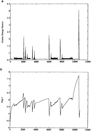
FIGURE 1
(a) Kinetic energy density (10-1 kg m-1 s-2); (b) basin mean temperature (°C) throughout one of the single-hemisphere integrations of Weaver and Sarachik (1991a). The sharp peaks in (a) and (b) represent the occurrence of flushes, whereas the more rapid oscillations indicate decadal variability. (From Weaver and Sarachik, 1991a; reprinted with permission of the American Meteorological Society.)
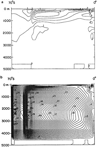
FIGURE 2
(a) Collapsed thermohaline state corresponding to year 1971 (refer to Figure 1) immediately before the flush shown in (b) at year 2067. All contours are in Sv; 1 Sv = 106 m3 s-1. (From Weaver and Sarachik, 1991a; reprinted with permission of the American Meteorological Society.)
the occurrence of flushes was resolved by Weaver et al. (1993). They showed that the existence of flushes is linked to both the importance of fresh-water flux relative to thermal forcing and the strength of the wind forcing compared to the high-latitude freshening. The latter balance was also investigated in detail in Marotzke (1990). Comparing the equilibria obtained under restoring boundary conditions with and without wind, he found that at middle and high latitudes the thermohaline circulation provided the dominant transport mechanism for the meridional fluxes of heat and salt. Moreover, the strength of the meridional overturning was little influenced by the wind field, except for the Ekman transport in the top layer and its return flow, which takes place in the 200 meters below the top layer. Because the stratification is nearly homogeneous in near-surface layers at high latitudes, the Ekman cells (i.e., Ekman transport plus return flow) contribute very little to the meridional
transports. The situation changes, however, after the polar halocline catastrophe has occurred in, for example, the Northern Hemisphere: The surface layer is very fresh, compared to the layers below, but the northward transport of more saline water compensates for the southward Ekman transport of very fresh-water, resulting in a net northward transport of salt. Moreover, the northward salt transport due to the horizontal subtropical gyre increases substantially during the collapsed phase of the thermohaline overturning.
When the thermohaline circulation has collapsed, the wind-driven northward transport of salt amounts to about half the value of the total transport for the spun-up steady state. Thus, the high-latitude surface freshening is counteracted by the wind-driven salt transport, which in the case of Marotzke (1989, 1990) was strong enough to make the high-latitude surface waters sufficiently saline again that deep convection resumed and the thermohaline circulation reestablished itself. Strong surface freshening (as in Weaver and Sarachik, 1991a) cannot be compensated for by the wind-driven salt transport, and the thermohaline circulation remains in the collapsed state until a flush sets in.
Weaver et al. (1993) further examined the robustness of these flushes in the presence of a stochastic term added to the imposed surface fresh-water flux field. In particular, they showed that as the magnitude of the stochastic term increased, the frequency of the flushing events increased, while their intensity decreased. When there was no stochastic forcing, deep-ocean temperatures warmed up to about 9°C in their model before static instability appeared at high latitudes, inducing convection and a flush. With the inclusion of a stochastic term in the fresh-water forcing field, flushes tended to occur earlier, before the ocean had warmed as much, and even earlier still as the magnitude of the stochastic forcing was increased. With increasing magnitude of the stochastic fresh-water flux forcing, there is an increasing probability that an evaporation anomaly will occur that is sufficiently large to induce convection and hence the onset of a flush. The basin mean temperature will not have warmed as much, so the ocean will lose less heat during the (thus weaker) flushing event. A similar result regarding the frequency and intensity of flushes was found when a seasonal cycle was imposed on the fresh-water flux field (Myers and Weaver, 1992).
Century-Time-Scale Overturning Variability
The time scale between the aforementioned flushes is diffusive and hence long (hundreds to thousands of years). A second fundamental period for variability occurs on the overturning time scale (Mikolajewicz and Maier-Reimer, 1990; Weaver et al., 1993; Winton and Sarachik, 1993). Mikolajewicz and Maier-Reimer (1990), in an uncoupled global ocean model that was driven by mixed surface boundary conditions and wind stress and to which a stochastic freshwater-flux forcing term had been added, found internal variability with a dominant period of 320 years (their overturning time scale). This variability was manifested in salinity anomalies, which they traced around the overturning gyre of the Atlantic Ocean.
Winton and Sarachik (1993), in a planetary geostrophic ocean model (where the velocity field is exactly geostrophic), obtained similar 350-year variability; they interpreted the oscillation as a manifestation of a large-scale Howard-Malkus loop oscillation (as described by Welander, 1986). They argued that the presence of a positive salinity anomaly in the low-latitude surface regions would tend to slow the meridional overturning slightly, since thermal effects tend to accelerate the thermohaline circulation and haline effects to brake it. The weakened thermohaline circulation would then be more affected by the specified flux on salinity, which would act to intensify the positive anomaly at low latitudes and induce a negative salt anomaly at high latitudes. When the low-latitude salinity anomaly reached the high latitudes, convection and an intensified thermohaline circulation would ensue. The whole process would begin a new when the saline anomaly resurfaced at low latitudes. Thus their oscillation had a rapid phase, which was associated with the saline anomaly's being at low latitudes, and a slow phase in which the salinity anomaly was at high latitudes or in the deep ocean. This oscillation may well be linked to the 350-year period variability found in the Cape Century ice-core records of Dansgaard et al. (1970), discussed earlier.
Weaver et al. (1993) also found variability of overturning time scale in their runs, which were conducted in a thermally dominant regime. That is, if the surface fresh-water flux forcing field was sufficiently weak that it played only a minor role in driving the thermohaline circulation, the only thermohaline variability that existed under a stochastically forced regime was on the overturning time scale. This variability is analogous to the loop oscillation of Winton and Sarachik (1993).
Decadal and Interdecadal Time-Scale Variability
In many of the long time integrations of Weaver and Sarachik (1991a,b) under mixed boundary conditions (see, e.g., Figure 1a), self-sustained internal variability on the decadal-to-interdecadal time scale was found. This variability was linked to the turning on and shutting off of high-latitude convection and the subsequent generation and removal of east-west steric height gradients that caused the thermohaline circulation to intensify and weaken on a decadal time scale (Weaver and Sarachik, 1991b). They showed that this variability was associated with the propagation to the eastern boundary of warm, saline anomalies, generated in a localized region of net evaporation in the mid-ocean, between the subpolar and subtropical gyres. The
separated western boundary current provided the source of warm, saline water required to initiate the anomaly development. Advection set the oscillation time scale, which was given by the length of time it took a particle to be advected from the mid-ocean region, between the subpolar and subtropical gyres, to the eastern boundary and then, as subsurface flow, toward the polar boundary. In more complicated geometry, they argued, one would expect this time scale to be slightly longer since the advective paths would no longer be along straight lines.
Figure 3, from Weaver and Sarachik (1991b), illustrates the meridional overturning stream function throughout the course of one particular oscillation in a single, Southern Hemisphere basin. During the oscillation the poleward heat transport changed by as much as a factor of 3 at certain latitudes. For example, at 26°S, during the most intense stage of the oscillation (Figure 3d) 0.29 petawatts (1 petawatt = 1015 W) of heat was being transported poleward, whereas during the weakest phase (Figure 3h) this was reduced to only 0.11 petawatts. The changes in heat transport corresponded directly to changes in the heat lost to the overlying atmosphere at high latitudes, since the ocean stored little heat during the oscillation. If such internal variability were to exist in the real ocean, it would evidently have a profound effect on global climate.
Weaver et al. (1991) attempted to understand why Marotzke (1989, 1990, 1991) and Marotzke and Willebrand (1991) almost never saw such spontaneous internal decadal oceanic variability (although one of the two-basin experiments described in Marotzke (1990) indicated the presence of decadal-to-interdecadal-scale oscillations in the region of the Antarctic Circumpolar Current), whereas Weaver and Sarachik (1991a,b) almost always found such variability. Through a systematic analysis of the forcing fields used in these works, they concluded that the presence of decadal-to-interdecadal variability was linked to an area of negative P - E at middle to high latitudes, and fresh-water gain further north. The meridional gradients in the fresh-water flux forcing field also had to be sufficiently strong that the system was in a haline-dominant regime. Figure 4a illustrates the basin-averaged surface heat flux over the course of the integration of one of the single-hemisphere experiments of Weaver et al. (1991), while Figure 4b shows the power spectral density of this curve over the first 8,214 years of integration. What is readily evident from this figure is that the dominant variability is in the decadal band, with associated basin-averaged surface heat-flux anomalies of between + 6 and - 10 W m-2 over one oscillation. Although the integration shown in Figure 4a eventually reached a steady state, Weaver et al. (1993) showed that the inclusion of a stochastic component in the fresh-water flux forcing field continually excited the decadal variability, with the result that no equilibrium was ever reached.
Weaver et al. (1991) suggested that when the thermoha-
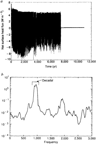
FIGURE 4
(a) Net basin averaged surface heat flux in W m-2 throughout the haline-dominated integration of Weaver et al. (1991). (b) Power spectral density (using a 256-point fast Fourier transform) of the surface heat-flux curve shown in (a) for the first 8,214 years of integration. The x-axis in (b) corresponds to the number of cycles over the 8,214 years of integration. (From Weaver et al., 1991; reprinted with permission of Macmillan Magazines, Ltd.)
line circulation was weak, it slowly passed through the region with negative P - E, and hence the surface waters became more saline. A warm, saline surface anomaly then developed through convection, and this anomaly was advected to the eastern boundary by the mean flow, from which it was convected to the deeper ocean (as in Weaver and Sarachik, 1991b). This led to the subsequent generation of the reverse cell seen in Figures 3a and 3b and Figures 3i and 3j, which in turn caused the thermohaline circulation to intensify. The intensified thermohaline circulation passed rapidly through the evaporative region; hence, the surface waters did not become as saline. Deep water then formed at high latitudes until high-latitude freshening dominated and the thermohaline circulation slowed down. This whole process repeated itself, with the time scale of the oscillation
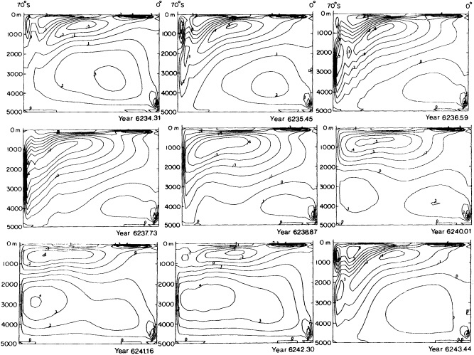
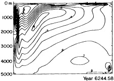
FIGURE 3
Meridional overturning stream function (in sverdrups) throughout one particular decadal oscillation. The plots are shown at 1.14-year intervals, and the period of the oscillation is 8.4 years. Positive contours indicate a clockwise transport. (From Weaver and Sarachik, 1991b; reprinted with permission of the Canadian Oceanographic and Meteorological Society.)
again determined by the time needed for salinity and temperature anomalies, formed in the local evaporative region, to be advected to the northern boundary.
The aforementioned OGCM simulations used time-invariant surface forcing fields (recall that the actual heat flux is time-varying but the restoring temperatures are fixed). In reality the oceanic surface forcing is not steady; apart from the seasonal cycle, the atmosphere and ocean are continually interacting with each other on small space and time scales. Weaver et al. (1993) considered these latter interactions as stochastic perturbations of the background forcing fields. They showed that the decadal internal variability still persisted when a stochastic component was added to the fresh-water forcing. Furthermore, Myers and Weaver (1992) showed that seasonally varying the surface forcing did not substantially alter the results.
The internal decadal variability discussed above is not limited to single-hemisphere, idealized ocean models. As shown by Weaver and Sarachik (1991 a), in two hemispheres under symmetric (with respect to the equator) forcing, deca-
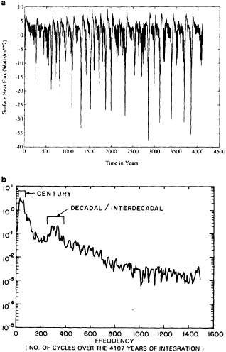
FIGURE 5
(a) Net basin averaged surface heat flux in W m-2 as a function of time for the stochastically forced experiment of Weaver et al. (1993). (b) Power spectral density (using a 512-point fast Fourier transform) of the surface heat-flux curve shown in (a) for the first 4,107 years of integration. (From Weaver et al., 1993; reprinted with permission of the American Meteorological Society.)
dal variability could occur in either hemisphere, essentially independent of the other hemisphere. Furthermore, in some of the two-basin results of Hughes and Weaver (1994), decadal-to-interdecadal variability was observed in either the North Atlantic or southern oceans, depending on the form of the fresh-water flux forcing field.
Combined Decade-to-Century Thermohaline Variability
As a final example of the type of variability that can exist in idealized OGCMs of the thermohaline circulation, the results of one of the experiments of Weaver et al. (1993) are presented. In this single-hemisphere experiment a stochastic term was added to the mean fresh-water flux forcing field. In the absence of stochastic forcing, the mean
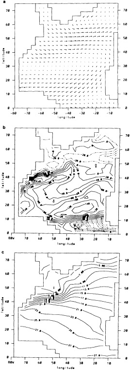
FIGURE 6
Forcing fields used to drive the 3° × 3° North Atlantic OGCM. (a) Hellerman and Rosenstein (1983) annual mean surface wind stress in dynes cm-2; (b) annual mean fresh-water flux field of Schmitt et al. (1989) in cm/yr; (c) Levitus (1982) annual mean sea surface temperature in °C. The maximum vector shown in (a) corresponds to 1.5 dynes cm-2.
fresh-water flux forcing field led to the occurrence of quasi-periodic intense flushing events on which was superimposed very weak decadal-to-interdecadal variability. Weaver et al. set the standard deviation of the fresh-water flux to 80 mm per month, which is equal to the globally averaged annual mean precipitation (Baumgartner and Reichel, 1975).
Figure 5a illustrates the net basin-averaged surface heat flux throughout the 4,107 years of integration, while Figure 5b is the power spectral density of the curve shown in Figure 5a. What is readily evident is that variability on numerous time scales is present. Strong decadal-to-interdecadal variability is superimposed on flushes and loop oscillations, yielding a time series that looks chaotic. In a two- hemisphere version of this experiment, a similar pattern occurred.
It is tempting to speculate that the thermohaline circulation of the real ocean might behave in a manner similar to this stochastic forcing experiment. That is, transitions would be occurring between states with relatively strong and relatively weak thermohaline circulations; superimposed on this one might expect background decadal variability with moderate flushing events. This suggests the possibility that a major source of decade-to-century climatic variability resides in the intrinsic dynamics of the ocean's thermohaline circulation. Moreover, the chaotic behavior observed in Figure 5a would make the ocean circulation essentially unpredictable on climatic time scales.
INTERDECADAL VARIABILITY IN A COARSE-RESOLUTION MODEL OF THE NORTH ATLANTIC
The OGCMs discussed in the previous section were largely restricted to idealized flat-bottomed basins forced by zonally averaged restoring temperatures, idealized winds (with no meridional component), and P - E fluxes diagnosed from equilibria obtained under restoring boundary conditions. A natural question that arises is: Does this variability carry over to more realistic GCMs that incorporate irregular coastlines, topography, and more realistic surface forcing fields? The purpose of this section is to present some recent simulations of the North Atlantic thermohaline circulation driven by realistic forcing fields.
Description of the Numerical Model
The model used is the Cox (1984) version of the Bryan-Cox OGCM as described by Weaver et al. (1994). The resolution of the model is 3° × 3°, with 20 vertical levels ranging in thickness from 50 m at the surface to 300 m at the bottom of the basin. In experiments I to 5 the basin is assumed to be flat-bottomed with a depth of 4,020 m. In experiments T1 to T3 bottom topography is incorporated into the model.
The model was driven at the surface by the Hellerman and Rosenstein (1983) annual mean North Atlantic wind-stress field (Figure 6a), Schmitt et al. (1989) annual mean fresh-water fluxes (Figure 6b), and by restoring the SST to the Levitus (1982) annual mean climatology (Figure 6c) with a 50-day time scale. The P - E field was converted to a salt-flux field using equation (3), with S0 chosen to be equal to the basin-averaged salinity (35.12 psu) of the North Atlantic Ocean as calculated from the data of Levitus (1982).
Over the top 210 m of the northern boundary either 0.0, 0.1, or 0.2 Sv of Arctic fresh-water flux was incorporated. The residual of the net evaporation from the Schmitt et al. (1989) data less the fresh-water flux through the northern boundary was added as an additional fresh-water source throughout the top 210 m at the equatorial boundary. This was done in order to keep the basin mean salinity constant throughout all integrations.
Table 1 lists the distinguishing characteristics of all eight
TABLE 1 Characteristics of Eight Experiments with a Coarse-Resolution Model of the North Atlantic*
|
Experiment Number |
Arctic Flux in Sv |
Where Arctic Flux was Applied |
Topography |
Internal Variability? |
Period of Variability |
|
1 |
0.0 |
N/A |
flat |
yes |
22 years |
|
2 |
0.1 |
Labrador + GIN** Seas |
flat |
no |
N/A |
|
3 |
0.2 |
Labrador + GIN Seas |
flat |
no |
N/A |
|
4 |
0.1 |
GIN Seas |
flat |
yes |
17 years |
|
5 |
0.1 |
East Greenland Current |
flat |
yes |
17 years |
|
T1 |
0.1 |
East Greenland Current |
full |
no |
N/A |
|
T2 |
0.1 |
East Greenland Current |
dredge of Labrador Sea |
yes |
17 years |
|
T3 |
0.1 |
East Greenland Current |
flat + full Labrador Sea |
no |
N/A |
|
* Details of these experiments in interdecadal variability can be found in Weaver et al. (1994). ** GIN stands for Greenland, Iceland, and Norwegian |
|||||
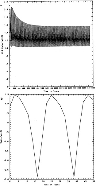
FIGURE 7
(a) Kinetic energy density (10-1 kg m-1 s-2) throughout the entire integration of experiment 1; (b) basin mean surface heat flux (in W m-2) during the last 49 years of integration of experiment 1. Notice that in (b) two complete 22-year period oscillations are resolved. Positive contours indicate that the ocean is gaining heat.
experiments; a more detailed discussion of the model used may be found in Weaver et al. (1994).
Interdecadal Variability of the North Atlantic Thermohaline Circulation
In this and the next subsection, attention is focused on experiment 1, in which there was no parameterization of
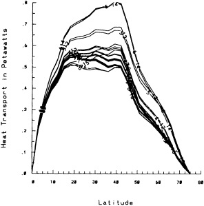
Arctic fresh-water input into the North Atlantic (see Table 1). Figure 7a shows the kinetic-energy density of the model ocean throughout the 3,472 years of integration. What is readily evident from this time series is that the system very rapidly entered a limit cycle, the period of which is about 22 years (Figure 7b).
Over the course of the oscillation the poleward heat transport varied from a maximum of about 0.8 petawatts at 39°N to a minimum of 0.5 petawatts (Figure 8). This change was associated with the shutting off and turning off of deep-water formation at the northern boundary of the Labrador Sea.
Figures 9 and 10 show the meridional overturning in the whole North Atlantic and in the Labrador Sea region, respectively. Plots are shown at the weak phase (Figures 9a and 10a) and strong phase (Figures 9b and 10b) of the oscillation. In the weak phase about 16 Sv of deep water is forming, about 8 Sv of it in the Labrador Sea near 63°N. Gradients in the stream function, and hence the vertical and meridional velocity, are relatively weak at this phase in the oscillation; the energy of the system (Figure 7a) and the poleward heat transport (Figure 8, lines 8 and 16) are therefore at a minimum. The ocean basin is also beginning to slowly take up the heat that it lost in the rapid phase of the oscillation (Figure 7b). As the thermohaline circulation in the Labrador Sea intensifies, so does the poleward heat transport (Figure 8), until deep-water formation is suddenly triggered at the northern boundary of the Labrador Sea (Figures 9b and 10b). At this stage the thermohaline circula-
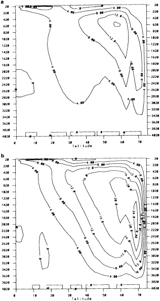
FIGURE 9
Meridional overturning stream function (Sv) for the whole North Atlantic basin throughout one particular interdecadal oscillation. The two plots correspond to the (a) weak phase and (b) strong phase of the oscillation. The year in the title of each figure corresponds to the x-axis of Figure 7b.
tion is most intense (Figure 7a), as is its associated poleward heat transport (Figure 8, lines 6 and 14). Furthermore, the heat that the ocean had gained over the previous 13 years is rapidly lost to the overlying atmosphere (Figure 7b).
Mechanism and Time Scale of the Variability
The discussion of the physical mechanism and time scales involved in the oscillation begins from the weakest phase
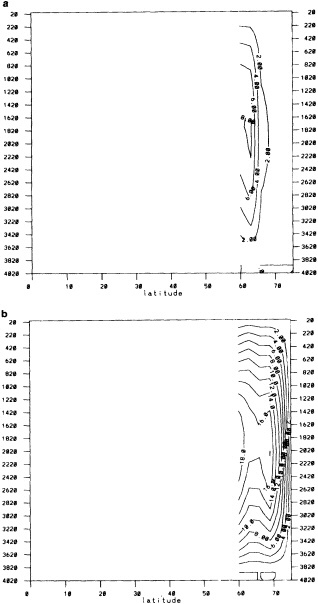
FIGURE 10
Meridional overturning stream function (Sv) for only the Labrador Sea region of the model domain throughout one particular interdecadal oscillation. The two plots correspond to the (a) weak phase and (b) strong phase of the oscillation. The year in the title of each figure corresponds to the x-axis of Figure 7b.
of the oscillation. The mechanism for the oscillation is quite different from that found by Weaver and Sarachik (1991b) and Weaver et al. (1991).
At the weak phase of the oscillation there is thermally driven deep convection all across the Labrador Sea (Figure 11a); hence, there is a very weak east-west pressure gradient. Consequently, the meridional geostrophic flow is weak at very high latitudes in the Labrador Sea, so there is no overturning there (Figure 10a). There is still a strong north-
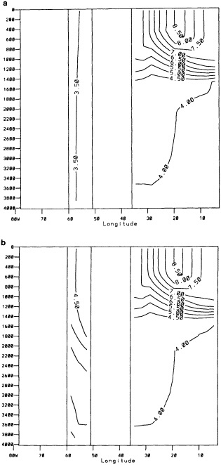
FIGURE 11
Horizontal section of potential temperature at 64.5°N at the (a) weak phase and (b) strong phase of the oscillation. The year in the title of each figure corresponds to the x-axis of Figure 7b.
south pressure gradient due to the surface restoring boundary condition on temperature (Figure 12a). Associated with this north-south pressure gradient is a zonal flow (Figure 13a) that converges at the western boundary of Greenland (near 66°N), causing sinking there and a return deep zonal flow below (Figure 14a).
The meridional velocity field converges on the boundary
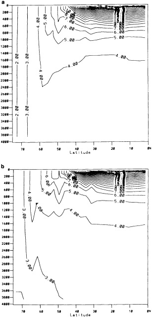
FIGURE 12
Meridional section of potential temperature at the first grid point ( 1.5°) off the western boundary of the model domain (see Figure 6). The figures correspond to the (a) weak phase and (b) strong phase of the oscillation. The year in the title of each figure corresponds to the x-axis of Figure 7b.
at the tip of Greenland, so at this stage the main component Labrador Sea overturning is formed between 60° and 63°N. Notice that during the previous strong phase of the oscillation, warm saline waters are brought into the Labrador Sea. The surface boundary conditions remove SST anomalies faster than they remove SSS anomalies; hence, the net surface density gradient during the weak phase still increases
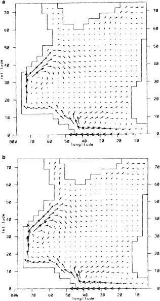
FIGURE 13
Horizontal-velocity field at the top model level at the (a) weak phase and (b) strong phase of the oscillation. The year in the title of each figure corresponds to the x-axis of Figure 7b.
as one progresses northward into the Labrador Sea, because temperature gradients dominate over salinity gradients. Since the SST and SSS are nearly zonally uniform, and convection penetrates to the bottom of the basin, there is only a very weak east-west pressure gradient in this weak phase. Deep water therefore does not form at the northern boundary. Overturning in the Greenland-Iceland-Norwegian seas now dominates the total overturning at high latitudes (Figure 9a).
The surface restoring boundary condition on temperature is given by equation (1) with ![]() replaced by the Levitus
replaced by the Levitus
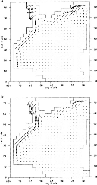
FIGURE 14
Horizontal-velocity field at a depth of 2970 m at the (a) weak phase and (b) strong phase of the oscillation. The year in the title of each figure corresponds to the x-axis of Figure 7b.
(1982) annual mean SST, ![]() (Figure 6c), together with a restoring time scale of tR = 50 days. During the intermediate phase of the oscillation, the warm saline waters in the high-latitude region of the Labrador Sea are being cooled toward the Levitus climatological temperature. Since convection extends to the bottom of the basin in the Labrador Sea on a rapid time scale (H2/ATV ˜ 1/2 year for average basin depth H = 4020 m and vertical diffusivity ATV= 104 cm2 s-1) condition (1) is equivalent to restoring the 4020 m deep basin to the surface value with an e-folding time scale of 11 years (assuming T1- TL is constant). Thus
(Figure 6c), together with a restoring time scale of tR = 50 days. During the intermediate phase of the oscillation, the warm saline waters in the high-latitude region of the Labrador Sea are being cooled toward the Levitus climatological temperature. Since convection extends to the bottom of the basin in the Labrador Sea on a rapid time scale (H2/ATV ˜ 1/2 year for average basin depth H = 4020 m and vertical diffusivity ATV= 104 cm2 s-1) condition (1) is equivalent to restoring the 4020 m deep basin to the surface value with an e-folding time scale of 11 years (assuming T1- TL is constant). Thus
during this 11-year period, the entire northern region of the Labrador Sea is being cooled from top to bottom.
As the high-latitude region of the Labrador Sea is cooled, the meridional surface pressure gradient increases, since temperature gradients dominate over salinity gradients as in the weak phase. This increasing meridional pressure gradient implies an increasing zonal overturning, which, through divergence (and hence upwelling) at the western boundary and convergence (and hence downwelling) at the eastern boundary, leads to an enhanced zonal pressure gradient and hence an enhanced meridional overturning.
The time scale for the set-up of the zonal pressure gradient is linked to the zonal overturning time scale in the Labrador Sea, which, assuming a 10 cm s-1 surface current, 1 cm s-1 deep return flow, and vertical velocities of the order of 0.01 cm s-1 (from figures not shown), is about 4 years.
As the meridional overturning begins to increase slightly at high latitudes, the cold and now fresh-water starts to move slowly equatorward in a deep western boundary current. Once this cold water has traveled a few degrees southward it suddenly shuts off convection from below at the western boundary (e.g., Figure 11b), because the cold fresh deep water is denser than the overlying warm saline water. The zonal pressure gradient is then further enhanced; hence, the overturning strengthens even further. The time scale for this southward advection of this cold fresh-water is approximately 1 year, assuming an advective speed of 2 cm s-1 over a distance of 600 km.
Once convection is shut off in the west, the overturning starts to increase rapidly, and the cold fresh high-latitude water mass is advected equatorward (in a deep western boundary current) and replaced by a warm salty water mass that originated in the surface waters at lower latitudes (Figure 12b). This is now the strong phase of the oscillation when the system is most energetic (Figure 7a), the heat loss is greatest (Figure 7b), and the poleward heat transport is the strongest (Figure 8, lines 6 and 14). Deep water is now forming at the northern boundary of the Labrador Sea (Figures 10b and 14b), and the flow in the Labrador Sea is strongest and oriented meridionally.
The time scale associated with the removal of the cold fresh high-latitude water mass and its replacement by the warm saline mass is linked to the overturning time scale in the Labrador Sea region. Assuming a 10 cm s-1 surface flow (Figure 13b), a 3 cm s-1 deep flow (Figure 14b) over a distance of 25° (that is, from the latitude where the western boundary current separates from the coast, 50°N (Figure 13b), to the northern boundary, 75°N), and a vertical velocity of 0.01 cm s-1, this time scale is about 5 years.
Since the deep basin of the Labrador Sea is now filled with warm saline water, convection from the surface to the bottom of the basin is induced everywhere through cooling to the Levitus SST field. Hence, the zonal pressure gradient that drives the enhanced thermohaline circulation is reduced, and the whole process begins again.
The total time scale of the oscillation according to the discussion above is therefore:
11 years—Time scale for the cooling of Labrador Sea
4 years—Time scale for Labrador Sea zonal overturning and subsequent set-up of meridional pressure gradient
1 year—Time scale for the equatorward advection of cold fresh-water in the deep western boundary current
5 years— Labrador overturning time scale for the replacement of cold fresh-water mass by warm saline-water mass
21 years— Approximate total time scale
This agrees fairly well with the period of 22 years found in the model solutions.
It should be noted that the time period required for the cooling of the Labrador Sea does not scale linearly with tR. For example, in an additional run that was performed with tR= 100 days instead of 50 days, the time scale of variability remained nearly the same (now 21 years). This might be expected, since T1- TL in the region of the Labrador Sea (Equation 1 with Ta= TL) was, on average, about twice as large as in the integration with tR= 50 days. As a result, (T1- TL)/tR and hence the heat flux out of the Labrador Sea were similar in both integrations. The remainder of the mechanism was identical to that discussed above, although deep ocean temperatures were warmer in the second case.
Role of Arctic Fresh-water Forcing and Topography
In experiments 2 through 5 a flux boundary condition was applied to the top 210 m of the northern boundary in order to parameterize a transport of fresh-water from the Arctic. Table 1 summarizes the location and magnitude of the flux that was applied. In experiments 2 and 3, in which a fresh-water source was added at the northern boundary of the Labrador Sea, the internal variability discussed in the last subsection was suppressed. The external freshening was so strong as to cap convection in the Labrador Sea, so the aforementioned mechanism for the variability could not occur.
If the 0.1 Sv was not spread all along the northern boundary, but concentrated only in the Greenland-Iceland-Norwegian seas region (experiment 4) or only in the two grid boxes next to the Greenland coast in the eastern North Atlantic (experiment 5), the variability still occurred, although on a slightly shorter time scale (17 years). In the case when Arctic fresh-water was put directly into the East Greenland Current region, the SSS field (not shown) did a fairly reasonable job of reproducing the climatological Levi-
tus SSS field, although it is clear that runoff from rivers, such as the Amazon and the St. Lawrence, and outflow from marginal seas, such as the Mediterranean, should be incorporated if one expects the Schmitt et al. (1989) P - E fields to drive a more realistic ocean climatology.
The role of bottom topography in the stability and variability of the thermohaline circulation also has not been treated adequately. Most of the uncoupled OGCM simulations described above assumed a flat ocean bottom. Moore and Reason (1993) suggest that some of the internal variability of the thermohaline circulation might be sensitive to the inclusion of bottom topography, although it is not clear how well this topography is resolved in their 12-level model. In experiments T1 to T3 bottom topography was incorporated into the model; the results are summarized in Table 1.
In experiment T1 full topography was used in the North Atlantic model. This topography had the effect of making the Labrador Sea everywhere less than 840 m deep. The net result was that the variability was suppressed. In experiment T2, the Labrador Sea region was dredged to be flat (4,020 m deep), with full topography elsewhere in the domain. In this case the variability reappeared with the same time scale and dynamics as in experiments 4 and 5. In the final experiment, experiment T3, the topography in the Labrador Sea region was left alone, and the rest of the ocean (with the exception of continental shelf regions) was dredged to be 4,020 m deep. The internal variability was once more suppressed.
The conclusions that one can draw from these experiments are limited. The Labrador Sea region is very poorly resolved (being only three tracer points wide); hence, the topography used was not representative of the region. Due to smoothing of the topography (continental shelf regions with deep ocean), the Labrador Sea ended up being far too shallow. Hence, deep convection, strong east-west pressure gradients, and a fully developed thermohaline circulation could not occur. Much finer horizontal resolution must be used before a more complete understanding of the role of topography can be obtained.
SUMMARY
From the foregoing discussion it is clear that in OGCMs forced by mixed boundary conditions, internal variability of the thermohaline circulation can exist on the decadal-to-millennial time scale. The most important component of the system-in fact, the one that ultimately determines the model's response-is the strength of the fresh-water flux forcing versus the thermal forcing. Of secondary importance is the strength of the fresh-water flux forcing versus the wind-driven salt transport. If the fresh-water flux forcing is weak, no internal variability exists. If the regime is haline dominated and high-latitude freshening dominates over the wind-driven northward salt transport, a polar halocline catastrophe and subsequent flushing events may set in. As shown by Weaver et al. (1993), for several P - E fields that differ well within the range of observational uncertainties, the thermohaline circulation in an OGCM responds in a completely different way. This has important implications for the interpretation and modeling of both paleo- and present climate and climate change. If the results of the idealized OGCMs hold for comprehensive climate models as well, a relatively small error in the fresh-water exchange between ocean and atmosphere may produce dramatic changes in the thermohaline circulation, with a significant impact on the global climate.
The models discussed above exhibit serious shortcomings in their formulation of the atmospheric coupling. For example, there is no feedback between the SST and the hydrological cycle; a warm SST anomaly should cause enhanced evaporation, which in turn would be likely to change the overall P - E pattern. If the thermohaline circulation is vigorous, heat transport is large and high-latitude SST should rise. The relative influence of the fresh-water flux forcing would thereby increase by comparison with the thermal forcing (which actually is given by the temperature contrast between high and low latitudes), which would tend to destabilize the state of vigorous meridional overturning. On the other hand, increased high-latitude SST leads to increased evaporation, and it is conceivable that the total atmospheric water-vapor transport from low to high latitudes would be reduced. This would reduce the high-latitude freshening and thus stabilize the thermohaline circulation. More modeling studies are needed to investigate the effect of a more realistic formulation of boundary conditions on an ocean-only model. In particular, one might expect that a realistic atmosphere would damp some of the oscillatory behavior discussed herein (e.g., Zhang et al., 1993). Nevertheless, a robust result of the above models is that spontaneous variability on a decadal or millennial time scale is possible in an ocean model, for a realistic set of parameters.
All of the long integrations that were discussed in this section were done using non-eddy-resolving ocean models without an ice component. It is not clear whether the spontaneous variability found in coarse-resolution models will carry over to more realistic eddy-resolving OGCM simulations. This is particularly worrying for the interdecadal variability found in the North Atlantic simulations. It was evident that the Labrador Sea was the most dynamically important region of the model, yet the resolution in the Labrador Sea was very coarse. Furthermore, feedbacks associated with a prognostic ice component coupled to an ocean model may act to stabilize the variability found in the OGCMs.
It is interesting to point out recent results from fully coupled atmosphere-ocean-ice GCM climate simulations being conducted at NOAA's Geophysical Fluid Dynamics Laboratory. The thermohaline circulation of the North
Atlantic Ocean (and the high-latitude air-sea-ice system in general) was found to undergo variability on the 30- to 50-year time scale in these long-term coupled integrations (Delworth et al., 1993). This result tends to lend credibility to the internal variability found in uncoupled OGCMs. It is not clear, however, to what extent the variability is preconditioned by the use of the flux-correction term in the coupled model. If the flux-correction term is large in magnitude and of a form that contains much high-latitude structure (as is the case in the flux-correction term used by Manabe and Stouffer, 1988—see their Figure A1), one might expect the oceanic variability to be determined by this structure, with the atmosphere providing a stochastic forcing that excites the variability. The high-latitude variability in the atmosphere and ice components of the climate system would then be forced by the internal thermohaline dynamics. This speculation follows from Weaver et al. (1993), in which it was shown that the internal variability in uncoupled ocean models was linked to the structure of the mean fresh-water flux field.
ACKNOWLEDGMENTS
The author acknowledges support in the form of NSERC, AES, DFO, and FCAR operating grants. I am also grateful to P. Myers and S. Aura for their assistance with some of the North Atlantic experiments, and to J. Marotzke for providing the Schmitt et al. (1989) P - E fields.
Commentary on the Paper of Weaver
EDWARD S. SARACHIK
University of Washington
I should like to comment first on the heat transport in Dr. Weaver's model. I remember that when Drs. Bryan and Lewis made their first global circulation model the heat transport was quite sluggish—less than a petawatt globally, I think. And in Dr. Weaver's Atlantic we have something of the order of 0.8 petawatt, basically because more than one heat source is sending cold water southward. So the branches of the thermohaline circulation really do seem to matter. There is sort of a general rule: The more sinking regions you accurately simulate, the higher the heat transport will be.
Maybe I can structure this discussion by raising some general questions. As you can tell, Dr. Weaver and I think alike, so he has mentioned some of them already. But I should like to re-emphasize that the reason we do all of this is that the thermohaline circulation really is very poorly observed. We have some time information from the paleo indicators, like what Keigwin and Lehman do—where they can see whether there is inflow into the Nordic seas 10,000 years ago, for example. There is sediment and tracer information where you can actually follow freons, 14C, and various other things around loops. But there is no measure, except very indirect ones, of vertical velocity. I feel that these sorts of models are the only way of getting real intuition about the kinds of circulations that are possible: in particular, thermohaline circulations. As we build up intuition about the types of circulations and types of variability possible, we develop a language to describe thermohaline circulations, and this language is then applicable to more realistic simulations. In fact, I think this progression could be seen in the papers we heard earlier today.
It seems to me that some general statements can be made. In these forced ocean models the variability increases when you switch to mixed boundary conditions; that is clear. No restoring-boundary-condition model has ever showed any instability, to my knowledge. As you increase the freedom to shut down and turn on the deep-water sources, you seem to get more variability. Just today, we have seen examples that Dr. Weaver showed of the Labrador deep source, and I suspect that if you put enough fresh-water into the south by some sort of melting process, you would find variability in the deep-water source in the Antarctic also.
The basic question, of course—one that involves the relevance of these sorts of forced ocean models to climate or to reality—is the coupling to the atmosphere. One way of phrasing it is, ''Do these oscillations continue to exist if you couple the ocean to an atmosphere?" Now you have to be very careful, because when you do couple it to a model atmosphere, you simply are not going to get the fluxes and the circulations that we get by using observed winds and observed salinities. It is a major problem of the atmospheric models that they do not rain in the right place, and it is a major problem of coupled atmosphere-ocean models in general that you have to make flux corrections in order to get the salinity of the upper ocean correct.
So the issue of how you answer the question is difficult. There will be coupled atmosphere-ocean models that will have variability or no variability, but they will not be coupled atmosphere-ocean models that have the same sort of forcing that you use to get the variability in the forced ocean models. Maybe we should do it the other way: Take the forcing from the coupled models and see whether the
forced ocean models have the same sort of variability, then answer the question of whether the atmosphere is stabilizing or destabilizing.
All the models we have seen are coarse-resolution models, not out of any deep feeling about what resolution to use but out of economic necessity and practicality. Dr. Barnett indicated the amount of data you get when you do global ocean models, although his was relatively coarse. It is just that these coarse-resolution models are manageable; they can actually be done on work stations, as Dr. Weaver's group and my group do.
It is hard to say whether the sensitivities of these models will be the same as those of higher-resolution models, because sensitivity tests simply have not been done for coarse-resolution models. But my own presentation clearly indicated the sensitivity to forcing. There will also be sensitivities to geography. The coarse-resolution, simplified sector models have used zonally symmetric forcing. When you use zonally asymmetric forcing, as Dr. Weaver did, you do get sinking in the Labrador Sea. Other factors are topography and ice. Since we are talking about fresh-water forcing, any process that contributes to fresh-water creation is important. It certainly seems that to do realistic simulations we will have to get all of those fresh-water processes correct.
Let me add some thoughts about what is going to happen in the future. Coupled atmosphere-ocean models will ultimately be the standard for looking at variability in the ocean. But it seems to me that they will not become so until the flux corrections are no longer needed. In other words, as the models get better, I expect the variability to become more believable.
The whole issue of eddies that Dr. McWilliams raised is one that I do not know how to deal with, because running eddy-resolving models is so complicated and time consuming. I do not expect to see comparable results from eddy-resolving models for another 10 or 20 years. At the moment we simply do not know how important eddies are for thermohaline variability.
Discussion
WEAVER: You'll find more topography results in my paper; I didn't have time to present them all. Topography is certainly important; when I put full topography into the entire ocean basin, it kills the variability. Dredge the Labrador Sea, and it comes back. But it's really a problem with the Labrador Sea, which is only three or four grid points wide in places; you end up smudging a 100-m shelf into a 3000-m ocean floor.
TALLEY: To get the overturning right on a global model, I think you need to consider salt sources, such as the Mediterranean. There's nothing similar in the Pacific.
GOODRICH: I wonder whether Peter Schlosser would care to comment on whether the areas of long-term convective shutdown he has observed resemble any of the mechanisms we've heard described in these modeling papers.
SCHLOSSER: It's really an 80 percent or so reduction of the deep-water formation rate in the Greenland Sea that began around 1980 and still persists, as far as we know. We don't know what drives this phenomenon. Among the speculations are a salinity change in the surface layers related to the return of the GSA to the Greenland Sea, and greater mixing of fresh-water from the East Greenland Current into the center. When we tried a similar assessment for the upper water column we saw hardly any trend over the period with the drastic deep-water change.
GHIL: I don't think that very high levels of stochastic forcing are compatible with true atmospheric forcing, and I don't find activating millennial flushes more often to be an appealing physical explanation of interdecadal variability.
Going to a more general question, what strategy can we use to validate some of these results, considering the rather poor set of observations we have?
WEAVER: On your first topic, I should perhaps explain that my decadal variability is not linked to the flushes; they occur in a separate, dominant period. It's in the century-to-millennial band that the flushes can be excited. On your second. I'd have to say that as a modeler I don't feel competent to design a field-observation comparison program.
DICKSON: Let me amplify Peter's point a bit. Although deep convection in the Greenland Sea does seem to have slowed down since 1980 when the GSA came back, there was an even greater fresh-water anomaly passing south along the east of Greenland in the 1960s as the GSA formed. But at that time the deep convection in the Greenland Sea was in full swing. It's difficult to understand how when it was undiluted it couldn't cap convection there. while now it's back in a diluted form it's offered as one explanation of capping convection in the Greenland Sea.
What concerns me is that people are starting to look at what they perceive to be recurrences of the GSA as the cause of change in the thermohaline circulation —which they in turn perceive to be driven by variations in deep-water formation in the Greenland Sea—and they're getting decadal fluctuations out of it as a result. I have a lot of problems with that; the main one is topographic: deep convection in the Greenland Sea simply doesn't get out, and there just isn't any convection to the bottom of the Labrador Sea at present.
Ed was right when he said that the problem is one of modeling
intermediate-water formation, which is very difficult, as Aagaard and Carmack noted. But if you truly want realism, you need to put in intermediate-water formation, the Greenland-Scotland Ridge, and the lack of convection to the bottom of the Labrador Sea.
SWIFT: As Bob mentioned, what affects the overflows may be more intermediate-water formation than deep-water. I'm not at all sure that there ever was deep convection in the Iceland Sea, at least in the present-day climate. My impression is that the GSA caused a freshening of the waters there involved in intermediate-depth convection, which meant that the Denmark Strait overflow freshened. Meanwhile, the fresh pulse rounded the tip of Greenland and mixed into the central Labrador Sea Water. The Iceland-Scotland Overflow Water probably took longer to respond to the fresh pulse, because a good deal of warm, salty Atlantic Water is resident at the sills and mixes with the outflow. The deep freshening signal is the sum of these components, each with a slightly different time of freshening.
MYSAK: Bob, is it true that convection was suppressed in the region of the Icelandic Sea, but not in the Greenland Sea, by the GSA?
DICKSON: Yes, it is. There is a tendency to call that area a gyre, but actually they are horses of a different feather. The Greenland, Icelandic, and Norwegian Seas are quite distinct, almost isolated. When the GSA caused salinity to drop below 34.7 in the area north of Iceland, suppressing deep convection, the peak convection in the Greenland Sea was still going like a train. I think Aagaard and Swift are right in saying that the Arctic intermediate water from the Icelandic Sea rarely moves over the convective center of the Greenland Sea.
ROOTH: I'd like to switch horses here, and ask Andrew a question. It's been proposed that for salt accumulation in subtropical gyres there is a critical temperature-salinity vertical-gradient ratio that allows 'salt fingers' (double diffusion) to preferentially transport salt down to intermediate- or deep-water levels. Do you know whether you are exceeding those salt-flux situations? And do you know whether anyone has used that as a constraint?
WEAVER: I must admit I've never checked that myself; I don't know whether anyone's looked into it.
CANE: I'd like to raise the issue of coarse resolution. It seems to me that it forces you to use—at least with the current numerical procedures—very high diffusivity characteristics, which will affect circulation stability. It's hard to say what that would mean when you can't get to a parameter range that resembles the real ocean.
Coarse resolution will generally suppress eddies, though Kirk's heat-transport results suggest that the resulting noise reduction might be a good thing. But then eddies are tied to mean circulation in ways that noise is not.
What worries me the most, though, is the necessity for simplifying the topography. Things move so slowly in the ocean when they don't have some slopes to rub up against.
The other thing I'd like to comment on is the question of coupling to the atmosphere. It seems to me that we might make one small step forward by replacing the ocean with a swamp-mixed layer and putting an atmospheric boundary layer on top of the ocean. It's difficult to calculate changes in the wind that way, or to do anything very convincing about precipitation changes, but you can get variations in heat flux and evaporation that way.
WEAVER: A Ph.D. student at the University of Victoria is taking a sector model, putting a simple thermodynamic ice model and a simple energy-balance model on top of it, and specifying some ad hoc hydrological cycle within it, as a first step toward the coupling you'd like to see. I agree with you entirely about the eddies and topography, but most of us just haven't the computing resources needed.
MCWILLIAMS: Let me add to the list of model-credibility questions the plausibility of the flushing modes. I think it might be worth looking at using some non-hydrostatic and, if you will, more defensible parameterizations of small-scale vertical fluxes.
Thermohaline Circulations and Variability in a Two-Hemisphere Sector Model of the Atlantic
DAVID MCDERMOTT AND EDWARD S. SARACHIK1
ABSTRACT
A coarse-resolution, simplified-geometry (sector) model of the Atlantic is described. Important features of this model include a Northern Hemisphere sinking region, a Southern Hemisphere sinking region, and a re-entrant channel to simulate the effects of the Antarctic Circumpolar Current. The circulation of the model ocean is described and diagnosed under restoring boundary conditions for both temperature and salinity. The model proves capable of simulating the grosser aspects of the deep-water Atlantic circulation. The variability of the thermohaline circulation under a switch to mixed boundary conditions (restoring on temperature and flux condition for salinity) is described.
INTRODUCTION
The thermohaline circulation (THC) of the Atlantic has a sinking branch, mostly in the Nordic seas and partly in the Labrador Sea, that puts cold water beneath the warm surface water. It also has a southern sinking branch, mostly in the Weddell Sea but partly in the Ross Sea. Cold, dense waters from these sinking regions spread out through the world ocean and are generally responsible for the maintenance of the stratification of the world oceans against the effects of heat diffusion from the surface. The export of cold water from high latitudes and its replacement by warmer surface waters implies a net heat transport toward the sinking regions: The THC is generally recognized as an important determinant of the mean climatic state of the earth's surface and overlying atmosphere.
The water from the Antarctic sinking region is extremely cold and relatively fresh, so when it sinks it is more compressible and therefore denser than the more saline deep water formed in the North Atlantic. The deep water formed in the Antarctic sinks to the bottom and becomes Antarctic Bottom Water (AABW, see Figure 1). The sinking from the Nordic seas becomes North Atlantic Deep Water (NADW), which overlies the AABW. Sector models with only one deep-water source cannot reproduce the interleaving of water masses seen in the deep ocean. Intermediate waters invade the ocean through wintertime convection and through the strong saline outflow of the Mediterranean. Intermediate water is much harder to simulate in a numerical model than deep water; this paper will concentrate on the deeper waters.
The water masses in the ocean can be identified by standard hydrographic measurements and by following the inputs of transient tracers at the surface through specialized
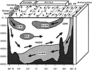
FIGURE 1
Schematic of water-mass distribution in the Atlantic (updated from Dietrich and Ulrich, 1968). AABW: Antarctic Bottom Water; NADW: North Atlantic Deep Water; CDW: Circumpolar Deep Water; SIW: Sub-Arctic Intermediate Water; AAIW: Antarctic Intermediate Water; MW: Mediterranean Water; PF: Polar Front; SC: Subtropical Convergence.
measurements; both give information about the broad outlines of the thermohaline circulation. The thermohaline circulation is characterized by extremely small velocities (especially vertical velocity), so direct measurement of the THC is impossible. Analytic and numerical models have therefore played a major role in our approach to understanding the THC. In particular, simple three-dimensional coarse-resolution sector models of the dynamics of the THC forced by steady mixed-boundary conditions (pioneered by F. Bryan, 1986a, 1986b) have begun to contribute a great deal to our understanding of the mean and variable THC.
Sector models contain the rudimentary dynamics needed to model the THC and its variability in a simplified context that allows many numerical experiments to be performed. On the other hand, the applicability of these simplified-model results to the real ocean will always be in question until they have been confirmed by experiments using more complex models with higher resolution, realistic geography and topography, and coupling to the cryosphere. Even then, the applicability of more complex forced ocean models to climate will be in doubt unless realistic, interactive coupling to the atmosphere can take place as well. (Fully coupled global atmosphere-ocean models are the ultimate tool for understanding the climate, but at present they are so expensive and complicated that they can be run only at a very small number of institutions.)
Coarse-resolution sector models have been used to investigate decadal and longer-term variability under steady mixed boundary conditions (see Weaver (1995), in this section, for a review and references). In sector models with two hemispheres, equatorially symmetric restoring boundary conditions on both temperature and salinity bring about a symmetric circulation with a sinking motion in the high latitudes of each hemisphere and a rising one at the equator. Upon a switch to mixed boundary conditions (restoring on temperature but with fluxes for fresh-water) asymmetric pole-to-pole circulations arise, with sinking in one hemisphere and rising in the other (F. Bryan, 1986b; Weaver and Sarachik, 1991a). With mixed boundary conditions (Weaver and Sarachik, 1991a), a transient chaotic state develops (in which symmetric circulations sometimes, though rarely, occur) that ultimately leads to a single asymmetric pole-to-pole steady-state circulation.
This paper presents a simplified model for investigating a more realistic geometry—one with a circumpolar current in one (the southern) hemisphere—in a sector context. Following a brief description of the model, the steady-state thermohaline circulations under restoring boundary conditions for both temperature and salinity are discussed, and then the variability of the model's physical quantities with a switch to mixed boundary conditions.
THE MODEL
The model used in the experiments described below is the Modular Ocean Model (MOM), a modular form of the Cox (1984) version of the Bryan-Cox Ocean General Circulation Model. The latter is a full primitive-equation model (in spherical coordinates) described by Bryan (1979) and Bryan and Lewis (1979). The MOM employs the finite-difference scheme described by Bryan (1969) and Cox (1984), and the polynomial approximation to the UNESCO equation of state described by Bryan and Cox (1972). We use a coarse horizontal resolution of 4° in latitude by 3.75° in longitude. The basin extends from 72°S to 72°N and is bound by meridians separated by 56.25° of longitude. A single re-entrant channel extends longitudinally 3.75° and latitudinally from 64°S to 48°S, and from the surface to a sill at approximately 2500 m depth. The basin depth ramps down from the sill depth to its full depth of 5000 m in the three grid spaces surrounding the channel opening, both to the north and south and to the east and west, and is uniformly 5000 m elsewhere. Vertical resolution is in 20 levels, so that numerical problems involving spurious circulations are avoided (Weaver and Sarachik, 1991a).
Cyclic boundary conditions are applied to the meridional boundaries at the slot, creating the re-entrant channel. Coarse-resolution models present difficulties in representing straits and narrow and silled channels. The B-grid used in the Cox-Bryan model requires a channel width of at least two tracer grid points to define one velocity point within the channel. As discussed in Toggweiler et al. (1989), the horizontal viscosity required to define boundary currents prevents a realistic flow from occurring in a channel that contains only one velocity point. We therefore create a re-
entrant channel that includes three velocity grid points and four tracer grid points.
The lateral walls and bottom all have insulating boundary conditions. A no-slip condition is applied at the walls, and the bottom is assumed to be impermeable. There is no bottom friction. The model uses the rigid-lid approximation at the surface in order to filter out high-frequency external gravity waves. The imposed surface wind stress, which is based on Hellerman and Rosenstein (1983), has only a zonal component. The zonal wind stress is shown in Figure 2b. The wind stress curl is anticyclonic between 15° and 45° latitude in each hemisphere and cyclonic elsewhere.
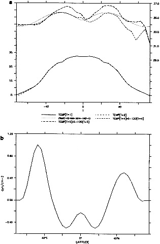
FIGURE 2
(a) The restoring temperature (lower curves) and salinity (upper curves) used in Experiments 1 and 2. The dashed temper- ature curve shows the slightly colder southern temperatures used in Experiment 2. The smooth (dotted) salinity curve, the restoring salinity used for Experiments I and 2, is a rough compromise between the dashed salinity curve (zonally averaged Atlantic curve from Levitus, 1982) and the dot-dashed salinity curve (zonally averaged world ocean salinity from Levitus, 1982). (b) The zonal wind stress applied in all experiments, in dynes/cm2.
The temperature is restored to prescribed values with a linear damping coefficient, with a time constant of 50 days. The reference temperature profile for the restoring boundary condition in Experiment 1 was obtained by averaging the world ocean values for Northern and Southern Hemisphere sea surface temperatures from Levitus (1982). In Experiment 2, the values for the Southern Ocean south of 50°S are lowered slightly in order to investigate the sensitivity of the circulation to the temperature of the sinking water. Both temperature profiles are shown in Figure 2a. In Experiments 1 and 2 the surface salinity is similarly restored to the idealized reference salinity values shown in Figure 2a.
To evaluate the salinity flux, Experiment 3 (mixed boundary conditions) used the equilibrium state of Experiment 1 but allowed it to run for an additional 50 years after the initial 7000-year integration utilized in Experiments 1 and 2. The surface salinity flux is averaged for that time period, and this average value is used to restart the model from the equilibrium state of Experiment 1. (This salinity flux is shown in Figure 9a.) The acceleration techniques of Bryan (1984) are used to speed the convergence of the model. The baroclinic velocity and barotropic vorticity equations are integrated with a time step of 2400 seconds, and the tracer equations are integrated with time steps of 4 days. The vertical eddy viscosity and vertical heat and salt diffusivity are set to 1.0 cm2/s everywhere. Horizontal eddy viscosity is set to 6 × 109 cm2/s, and horizontal tracer diffusivity is set to 1 × 107 cm2/s. The method of complete convection, the asymptotic limit of the diffusive convection parameterization, is used for all experiments. It has been described by Yin and Sarachik (1994).
THE STEADY THERMOHALINE CIRCULATION
Experiment 1. Symmetric Restoring Temperatures
Figure 3a shows the zonally averaged stream function for Experiment I under restoring boundary conditions on both temperature and salinity. Experiment 1 shows three distinct thermohaline cells: an Arctic cell 16 Sv in strength with sinking at the northern wall, an Antarctic cell over 6 Sv in strength with sinking at the southern wall, and a cell 6 Sv in strength with sinking on the north side of the re-entrant current and southward surface flow all the way from the equator. Surface-confined cells on either side of the equator, locally driven by the equatorial Ekman divergence caused by easterly trade winds, are also evident.
Note that the surface stream function between 30°N and 40°N is oriented northward when the winds at those latitudes are westerly, implying southward Ekman flow near the surface. Examination of the surface currents (Figure 4a) indicates that the southward branch of the zonally averaged stream function in Figure 3 is dominated by a southward boundary current, while the interior flow is northward in
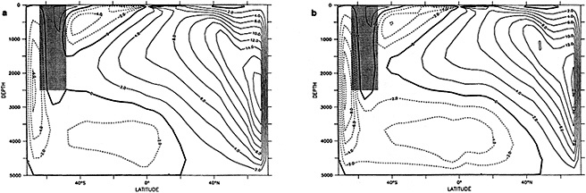
FIGURE 3
Zonally averaged stream function in sverdrups. (a) Experiment I with symmetric restoring conditions. (b) Experiment 2 with restoring to slightly colder southern temperatures. Clockwise circulations shown solid, anticlockwise shown dashed. Contour interval is 2 Sv. Shaded area indicates location of re-entrant channel.
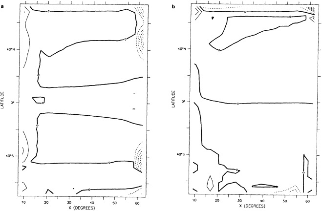
FIGURE 5
Vertical velocities from Experiment 1 (symmetric restoring temperature): (a) at 150 m, (b) near the bottom at 4800 m. Contour interval is 0.0005 cm/s.
the westerlies and southward in the easterlies, as expected. Similar considerations hold for a limited region of the surface stream function near 30°S.
Also disguised by the zonally averaged stream function shown in Figure 3a are the details of the mean sinking motion. Near the surface, there are three regions of sinking in the basin (Figure 5a). There is sinking along the entire northern boundary, joined to sinking along a considerable portion of the eastern boundary north of about 20°N. There is sinking in the southeast corner of the basin poleward of the slot. Finally, there is a sinking region on the eastern boundary in the Southern Hemisphere north of the slot: This is the sinking that corresponds to the shallow counterclockwise meridional cell in Figure 3a. Figure 5b shows that the only flow that reaches the bottom is the sinking along the northern wall, which is joined to intense sinking in the northeast corner of the basin, and a small region of sinking near the southeast corner.
Examination of the currents clarifies the movement of the water from those sinking regions in which water does not reach the bottom. Figure 4c shows the currents at 2000 m. The sinking water along the northern part of the eastern boundary feeds a westward current flowing along 50°N, which then becomes part of the deep southward-flowing western-boundary deep current. This broad current (about 11° of longitude) extends from about 1000 m down to the bottom while north of the equator, and from 1000 m down to only 4000 m from the equator to its termination at 20°S; it lies directly below the equally broad (in this coarse-resolution model) northward-flowing western-boundary current. Below 4000 m, the southward-flowing current turns eastward at the equator, leaving southward flow only above 4000 m. This remaining southward flow turns eastward at about 20°S and flows back across the basin to the eastern boundary.
The other region of shallow sinking (centered at 40°S just north of the slot on the eastern boundary) extends only to 1000 m. It feeds a westward-flowing current (Figure 4b), which ultimately turns northward above the southward-flowing western-boundary current.
The water that does reach the bottom along the entire northern boundary flows southward and westward upon reaching the bottom (Figure 4d). The negative vertical velocity, which goes to zero at the bottom, is accompanied by anticyclonic flow; the zero vertical velocity, which increases to positive values in the interior near-bottom upwelling regions, is accompanied (through the Sverdrup relation fwz= v) by cyclonic flow, in particular northward flow toward the northern sinking regions. The southern sinking water in the southeast corner of the basin reaches the bottom and flows northwestward. The near-bottom vertical velocity is downward and, again by the Sverdrup relation, implies northward motion.
The combination of the northward-flowing warm western-boundary current and the deeper southward-flowing cold western-boundary countercurrent produces a strong northward heat flux (Figure 6). This flux is consistent with the input of heat through the surface in low latitudes and the strong removal of heat at higher northern latitudes (Figure 9b). The vertically and zonally integrated meridional oceanic heat flux is northward north of 8°S; it has a peak value of 0.61 PW.
The eastward flow through the slot (the analog of the Antarctic Circumpolar Current) is relatively intense. The eastward flow, which extends below the sill to about 3000 m, is caused by westward-flowing deeper water's hitting the sill, upwelling, and returning eastward.
Barely evident in Figure 3a is the so called "Deacon Cell," a cell with rising motion at lower depths to the south of the re-entrant current, northward surface currents (consistent with westerly winds), and sinking still further north. This cell, which appears in more realistic ocean models that have geography and topography (Toggweiler et al., 1989), is responsible for bringing old 14C to the surface.
Experiment 2: Colder Southern Restoring Temperature
Figure 3b shows the zonally averaged stream function for Experiment 2, which has slightly colder restoring temperatures in the south (with 0.6°C maximum difference at the southern boundary). Compared to the results of Experiment 1, the Antarctic Cell has markedly increased in strength, and the apparent penetration of Antarctic Bottom Water has moved considerably northward. The northern thermohaline cell has weakened by 2 sverdrups.
Examination of the vertical velocities near the surface (Figure 7a) and near the bottom (Figure 7b) shows that in
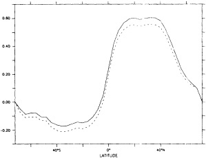
FIGURE 6
Zonally and vertically integrated meridional heat flux for Experiment 1 (solid line, symmetric restoring temperature) and Experiment 2 (dashed line, slightly colder southern temperature). Units are petawatts.
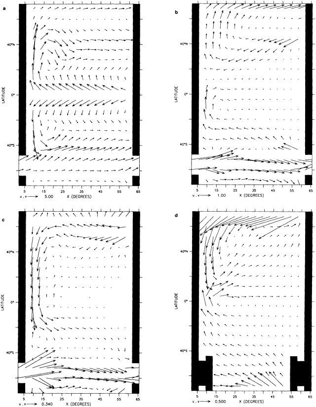
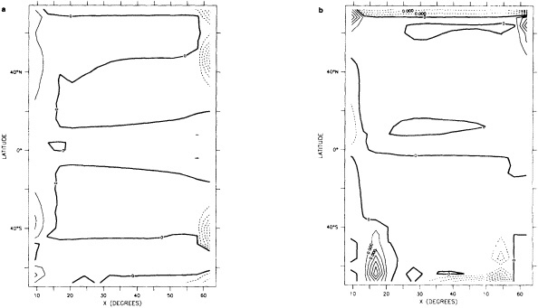
FIGURE 7
Vertical velocities from Experiment 2 (slightly colder southern restoring temperature): (a) at 150 m, (b) near the bottom at 4800 m. Contour interval is 0.0002 cm/s.
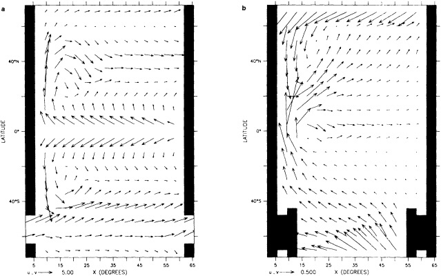
FIGURE 8
Currents from Experiment 2 (slightly colder southern restoring temperature): (a) near the surface (25 m), (b) near the bottom at 4800 m.
Experiment 2 the vertical velocities near the surface are similar to, but slightly stronger than, those in Experiment 1, and that the sinking velocities become much stronger with increasing depth. Although the sinking along the entire northern wall is a good deal stronger in Experiment 2 than in Experiment 1, the zonally averaged sinking is weaker (causing the weakening of the overturning stream function) because of the small region of upwelling in the northwest corner. As can be seen from Figure 7b, all the sinking is stronger in Experiment 2.
The stronger sinking at depth leads to stronger near-bottom currents. In particular, the water leaving the sinking region in the southeast corner of the basin flows northward and westward (Figure 8b), as it does in Experiment 1 (compare Figure 4d), but now creates a noticeable upwelling region against the ramp connected to the slot sill. It also flows further northward along the western boundary in the bottom thousand meters. This more northward penetration of bottom water shows up in the zonally averaged stream function as a more northward penetration of the southern overturning cell (Figure 3b compared to Figure 3a).
The more northward penetration of colder bottom water emanating from the sinking region in the southeast corner for Experiment 2 implies a more southward (or less northward) total heat flux. Figure 6 shows that this is indeed the case.
THERMOHALINE VARIABILITY
When the boundary conditions at the end of Experiment 1 are switched to mixed boundary conditions (i.e., conditions that restore the symmetric temperature profile and the diagnosed salinity fluxes shown in Figure 9a; we called this Experiment 3), strong haloclines form in both the Northern and the Southern Hemispheres, shutting off deep sinking in both regions. Intermediate water is formed north of the gap in the Southern Hemisphere, which moderates the diffusive warming of the deep ocean. As the deep ocean warms, the circulation exhibits a series of small-amplitude oscillations about 1400 years after the switch to mixed boundary conditions (see Figure 10a). The variability begins as fairly regular cycles with periods of just over four years, and the period is seen to decrease. After 450 years of oscillations the period is reduced to just over 3 years, and then for approximately 200 years the variability becomes increasingly irregular. The circulation then shifts to the steady state
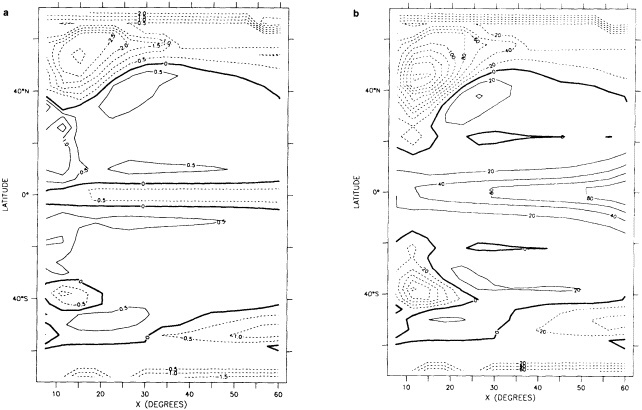
FIGURE 9
(a) The diagnosed salinity flux (converted to fresh-water flux in m/yr) from the equilibrium state of Experiment 1. Contour interval is 0.5 m/yr. (b) The heat flux through the surface for the equilibrium state of Experiment 1 in w/m2. Contour interval is 20 W/m2.
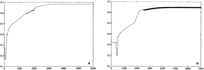
FIGURE 10
The kinetic energy per unit volume averaged over the entire ocean volume (units of 0.1 kg m-1 s-2) after the switch to mixed boundary conditions from the steady state of (a) Experiment 1 (symmetric restoring boundary conditions) and (b) Experiment 2 (cold south restoring boundary conditions).
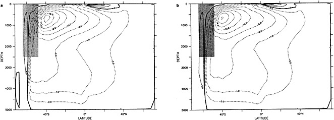
FIGURE 11
Zonally averaged steady-state stream function (in sverdrups). (a) Stream function corresponding to the steady state reached in Figure 10a. (b) Stream function corresponding to a time average over 30 years in Figure 10b. Contour interval 2 Sv. Shaded area indicates location of re-entrant channel.
shown in Figure 11. The high-latitude freshening is so large that sinking no longer occurs at high latitudes, and all the deep sinking occurs in the latitude of the slot in the Southern Hemisphere. Figure 11a may be considered the analog of the pole-to-pole circulation in the two-hemisphere symmetric case of Weaver and Sarachik (1991a), except that here the restoring salinity flux is itself asymmetric.
A closer look at the variability shows it to be most strongly evident in changes in convection in the western side of the basin at 58°S. Figure 12 shows contours of salinity at 58°S for four consecutive years. Throughout this period there is convection to the north of this latitude to about 2000 m, and a strong halocline capping the latitude band to the south. All deep convection is occurring at 58°S. In Figure 12a, the southern halocline extends to 58°S in the western part of the basin. Fresh surface water is advected northward to produce this cap, but convection continues at depth. One year later, in Figure 12b, we see the capped region has moved slightly eastward. The eastern edge of the capped region advances no further than this; as can be seen in Figure 12c, however, convection advances in the west, shrinking the size of the cap. At the end of the cycle, in Figure 12d, convection occurs across the basin at 58°S. Advection of fresh surface water in the west produces a capping of convection there, and the cycle continues.
When the salinity flux of Experiment 2 is diagnosed, we
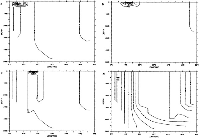
FIGURE 12
Vertical-longitudinal sections of salinity at 58°S in Experiment 3 for four consecutive years during the period of variability. Contour interval in (a) is 0.02 ppt, in (b) is 0.05 ppt, in (c) is 0.02 ppt, and in (d) is 0.01 ppt.
find the fluxes shown in Figure 13. Note that the fluxes are very similar to the fluxes diagnosed from Experiment 1 except near the southern boundary, where Experiment 2 convection is very much stronger (compare Figure 9). When the steady-state Experiment 2 is then switched to mixed boundary conditions (Experiment 4), the circulation undergoes the evolution shown in Figure 10b. The initial stages of the circulation are similar to those in Experiment 3, with the formation of strong haloclines in both northern and southern regions, and the initiation of intermediate-water formation at approximately the latitude of the gap. As this water formation strengthens and extends to become deepwater formation, the circulation develops a very regular 30-year oscillation. The overturning stream function averaged over one 30-year period is shown in Figure 11b.
The variability in Experiment 4 is also most strongly evident in changes in convection in the western side of the basin at 58°S. The extension of the southern halocline to 58°S latitude is shown in Figure 14. The strength of the stratification in this region varies over the course of the 30-year cycle, but convection from the surface breaks out only at the column located at 5.6°E and 58°S. As can be seen in Figure 15b, the resulting variability in overturning stream function is fairly small.
The surface forcing at this location comes from cooling and evaporation, both of which tend to destabilize the column. Advection brings cold fresh-water into the upper levels from the south. Figure 15a shows how the meridional velocity to the south of the variably convecting region changes through one cycle. The advection from the south decreases until convection from the surface begins (year 11) and then increases until the convection is shut off (year 19). The column upstream of this location (to the west) is convecting down to the sill depth. The water being advected from the west is vertically homogenous in temperature and salinity, and is both warmer and saltier than the water found in the column at 5.6°E and 58°S. This zonal velocity (not shown) into the location of convective variability decreases while convection occurs, and increases while convection is not occurring. While this oscillation has only a small effect on the large-scale overturning, local effects are significant. Figure 16 shows the surface heat flux in the region of convective variability over one 30-year cycle.
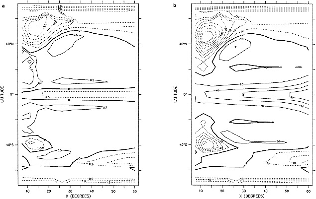
FIGURE 13
(a) The diagnosed salinity flux (converted to fresh-water flux in m/yr) for the equilibrium state of Experiment 2. Contour interval is 0.5 m/yr. (b) The heat flux through the surface for the equilibrium state of Experiment 2 in w/m2. Contour interval is 20 W/m2.
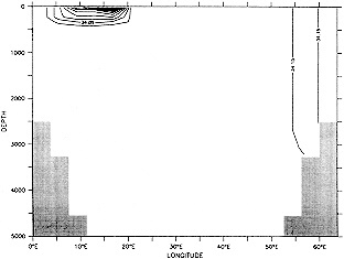
FIGURE 14
Vertical-longitudinal sections at 58°S of salinity in Experiment 4 at a time when cap extends to 5.6°E. Contour interval is 0.05 ppt.
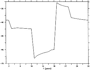
FIGURE 16
Surface heat flux for one cycle in region of convective variability, in W/m2.
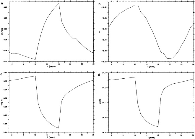
FIGURE 15
(a) Meridional velocity averaged over the top 112 m at 5.6°E, 62°S. (b) Minimum value of zonally averaged stream function (in sverdrups) during 30-year cycle (see Figure 11b). (c) Average temperature below 1500 m in region of convective variability. (d) Average salinity below 1500 m in region of convective variability, in ppt.
CONCLUSION
We have constructed an idealized model of the Atlantic basin and described the steady circulations that resulted from forcing under symmetric restoring boundary conditions (Experiment 1). A small reduction in restoring temperature in the Southern Hemisphere (Experiment 2) led to a rather significant change in the intensity of the vertical circulations. Upon a switch to mixed boundary conditions, the state produced by Experiment 1 progressed to a final steady state with only transient variability, while the state resulting from Experiment 2 settled into a regular oscillation with a period of approximately 30 years.
It has become clear that several different kinds of variability are possible under constant mixed boundary conditions. Each region of deep sinking in the ocean can be capped by fresh-water and can therefore be variable. Weaver (1995, in this section) shows that variability arising from the variability of the sinking region in the Labrador Sea involves processes different from variability arising from the variability that involves the sinking region in the Nordic Seas. Similarly, this paper shows variability involving the sinking region poleward of the Antarctic Circumpolar Current.
We conclude with some questions and qualifications of the above work.
The simple type of coarse-resolution sector model presented here has a number of features that resemble the real ocean, and therefore proves useful in isolating these processes for detailed study. In particular, we saw that a small change in the restoring temperature led to rather large changes in the thermohaline circulation, even at high northern latitudes, and to even larger changes in behavior under a switch to mixed boundary conditions. While we cannot yet explain this sensitivity, we note that such unexpected sensitivities, if shown to be realistic in more complex models, may have important climatological consequences.
The basic question that arises from this and all other
ocean-only models is what the effect of the atmosphere is on the variability. Coupling the atmosphere to the ocean in tropical models tends to induce instabilities that were not present in models of either the atmosphere or the ocean. Whether the atmosphere is stabilizing or destabilizing for the variability exhibited in ocean-only models must await detailed simulations with coupled atmosphere-ocean models.
ACKNOWLEDGMENTS
The authors are indebted to Michael Winton and Fenglin Yin for very helpful discussions, to Michael Ghil for a detailed reading of the first draft of this paper, and to Ed Harrison and Steve Hankin of NOAA/PMEL for the use of FERRET, a diagnostics and graphics program that was used extensively in this research. This work was supported as part of the Atlantic Climate Change Program by a grant from the NOAA/Office of Global Programs to the University of Washington Experimental Climate Forecast Center. David McDermott was also supported as a Graduate Fellow for Global Change by the Department of Energy, and part of this research was performed using the resources located at the Advanced Computing Laboratory of Los Alamos National Laboratory.
Commentary on the Paper of McDermott and Sarachik
MICHAEL GHIL
University of California, Los Angeles
I very much enjoyed this paper. However, it needs to be put into the broader context of the other papers on decade-to-century variability in the ocean's thermohaline circulation (THC) presented at this workshop. There is considerable activity going on in this area, and we will get together a small Climate System Modeling Program (CSMP) workshop at UCLA in October 1993 to clarify some of the issues further.
My view of the scientific method is that we proceed from detection of phenomena via understanding to simulation, and eventually on to prediction. There are some shortcuts, such as statistical predictions that try to circumvent understanding and simulation, but we have full confidence only when all the stages of this progression have been visited.
Now, this gradual approach to the entire cognitive process also implies that there should be a gradual approach to one particular step, which is the understanding of the models. So I would just like to refer you to a couple of relevant figures that are halfway between Dr. Bryan's 'toy' model and Dr. Sarachik's complex one (Figures 9, 14, and 16 of Quon and Ghil, 1992), and talk about the issue of multiple equilibria in such simple models, as touched upon by Claes Rooth.
It has been observed in a number of THC models of different complexity that, under symmetric forcing with respect to the equator, you can have either two-cell symmetric circulation or one-cell pole-to-pole circulation. My illustrations show that essentially you can have all the intermediate steps. In other words, you can go from the symmetric circulation to the completely antisymmetric one gradually. Actually, this is a more realistic approach to the Atlantic's THC, as presented in McDermott and Sarachik's Figure 1 (see also Figure 1 of Ghil et al., 1987). There is North Atlantic Deep Water (NADW) reaching into the high southern latitudes, but there is Antarctic Bottom Water (AABW) spreading under it past the equator. So while the Quon and Ghil (1992) model is only two-dimensional, it manages to capture this asymmetry (see Figure 9 there), with one cell (NADW) dominating the other (AABW) without suppressing the latter entirely.
The linear stability analysis for this highly resolved, albeit two-dimensional, model yields a regime diagram (Figure 14 of Quon and Ghil). This diagram demonstrates that increasing either the imposed pole-to-equator temperature gradient at the surface or the salinity flux across the boundary will produce a gradual transition between two-cell symmetric circulations and completely antisymmetric circulations. A gradual increase of the measure of asymmetry is thus possible. Mathematically, this gradual increase is captured by a pitchfork bifurcation (Figure 16 in Quon and Ghil).
Now, Dr. Sarachik started with symmetric forcing and then also imposed slightly asymmetric forcing. Actually, when these mixed boundary conditions were enforced, in one case the response of his model was to switch to another steady state; in the other case, it went to oscillatory behavior.
To conclude, I believe that oscillations shown by some of these ocean THC models or coupled atmosphere-ocean GCMs have something to do with the spectral peaks detected in global and local temperature series (e.g., Ghil and Vautard, 1991; also Cook et al., 1995, and Keeling and Whorf, 1995, both in this volume). We need to identify certain oscillations in the models with what we think we observe, since confronting models with observations is the name of the game in the physical sciences.
Discussion
DESER: What is the mechanism for beginning a new cycle of the eastward-moving salinity anomalies?
SARACHIK: The Antarctic Circumpolar Current is a re-entrant current in our model. But of course it's hard to say how any oscillation begins; there's no particular ''start" spot in the cycle.
PHILANDER: You mentioned that you were concerned about the consequences of a 0.6°C perturbation. Could it reflect a large change in the westerlies, via Ekman drift?
SARACHIK: Perhaps. What most concerns me is the sensitivity these sorts of model seem to exhibit. I'm wondering whether that's the result of something in the idealized configuration, the re-entrant current, or what.
CANE: Eli Tziperman and colleagues have done some work recently that relates to the time constants you put into the restoring terms for temperature and salinity and whether you go to a flux condition. In some sense, I think one of the characteristics of most of these ocean-model studies with time-constant forcing is that the atmosphere is perhaps not active enough. There are various ways of calculating the sensitivity of the heat flux to a change in surface temperature; except for the truly coupled GCMs, I think that the models tend to hold the atmosphere more fixed than is appropriate for its heat capacity, which makes the time shorter. If that were loosened up, and the time lengthened, we'd get somewhat different answers for all these cases—the points at which you go from stable to unstable behavior and the like.
Low-Frequency Ocean Variability Induced by Stochastic Forcing of Various Colors
TIM P. BARNETT,1 MING CHU,2 ROBERT W. WILDE,3 AND UWE MIKOLAJEWICZ4
ABSTRACT
A primitive-equation global ocean general-circulation model with realistic geography has been forced with a variety of fresh-water flux models. The models' response appears as a number of fundamental eigenmodes. If the high-latitude forcing is of the order of I to 2 mm/day, then the dominant response has a period of roughly 300 years with significant variability in all the world's oceans. This response, partially documented by Mikolajewicz and Maier-Reimer (1990, 1991), occurs for forcing that is red or white in space and white in frequency. The transport of the Circumpolar Current fluctuates in response to this mode by a factor of two. In the Atlantic, the mode has a meridional circulation that extends over the whole basin/water column and a horizontal circulation that is clockwise. The most energetic portion of the Pacific circulation is more closely confined to the surface and more confused, although the associated attractor is fairly regular.
INTRODUCTION
Increasing attention has been focused on the role of the ocean in forcing climate variations with time scales from decades to centuries. Among the various components of the global climate system, only the ocean seems at this stage of understanding to have the requisite thermal inertia. The atmosphere appears to have little memory beyond a few weeks, due to its small density and thermal capacity. Major changes in climate are associated with shifts in the planetary ice sheets, but the time scale of these changes is of the order of 1000 years or more, apparently too long for them to be a prime mechanism in forcing decade-to-century variations in other climate system components. Finally, changes in external forcing (e.g., solar radiation) and in some internal forcing (e.g., volcanoes) either have yet to be established or are currently thought to be too weak to affect other than local climate changes. The oceans thus remain as the most likely source of climate variability on time scales of 10 to 100 years or more.
Recent work by a number of climate modelers has suggested that modest changes in atmospheric forcing can lead to radical changes in oceanic circulation that could have a dramatic impact on the global heat balance. The pioneering study of Stommel (1961) was apparently the first to suggest that the ocean's thermohaline circulation could exist in different, but stable, states. A spate of recent work with more complex models has confirmed that early work (see the comprehensive review of Weaver et al., 1993) and revealed many of the properties of the state transitions, as well as the sensitivity of the model results to subtle changes in the specification of the forcing—in these cases the flux of fresh-water into and out of the oceans.
Most of the work to date has been done with simplified ocean models or steady-state fluxes of fresh-water. The important work of Mikolajewicz and Maier-Reimer (1990, 1991) added a stochastic forcing term in the fresh-water flux and also used a full three-dimensional ocean general-circulation model (OGCM). Their result showed a quasi-periodic fluctuation in the thermohaline circulation; it had a time scale of the order of 300 years, and was most apparent in the Atlantic Ocean. Stocker and Mysak (1992) find significant spectral peaks in paleoclimate data with about the same period. Recently, Weaver et al. (1993) and Mysak et al. (1993) repeated that experiment (with a more simplified OGCM and rather arbitrarily defined flux fields) and described the relative importance of the stochastic term to the general model behavior.
The current paper expands on these earlier studies by examining the response of a realistic OGCM to different types of stochastic forcing. The model response to purely climatological forcing is compared to the additional response induced by stochastic forcing that is (1) white in both space and time, (2) red in space and white in time, and (3) red in both space and time, with the degree of redness determined by the coupling coefficients between the sea-surface temperature (SST) and SST gradients and the fresh-water flux field. This represents a coupled ocean-atmosphere model of a type that does not seem to have been previously explored.
DESCRIPTION OF MODELS AND EXPERIMENTAL DESIGN
This section describes the ocean and stochastic atmospheric models used in this study. It also describes briefly how the coupled ocean-atmosphere model with feedback was constructed.
Ocean General-Circulation Model
The OGCM used here is identical to that used by Mikolajewicz and Maier-Reimer (1990, 1991; MMR hereafter), which is described in detail by Maier-Reimer et al. (1993). It is a linear, primitive-equation model with a horizontal resolution of approximately 3.5° (an E-type grid) and 11 levels in the vertical. Unlike most of the modeling studies discussed above, this OGCM uses realistic geometry and ocean bathymetry. This is an important characteristic if one wishes to infer that the model results have relevance to the real world. The numerics are handled in such a way as to allow a time step of 30 days, thereby making extended integration feasible even on a workstation. At the surface (only) the heat-balance equation has a seasonally varying Newtonian damping to observed surface air temperature climatology, while the salt balance uses a seasonally varying fresh-water flux to give realistic surface salinity fields (mixed boundary conditions). Seasonally varying wind stress (Hellerman and Rosenstein, 1983) is also used to force the model.
Again unlike most of the modeling work discussed above, the OGCM includes a simplified thermodynamic sea-ice model wherein the heat flux through the ice is proportional to the temperature difference between the underlying water and air temperature, and inversely proportional to the thickness of the ice. If one is interested in forcing an OGCM with fresh-water flux, then some representation of sea ice seems mandatory for a realistic simulation. In addition, the full UNESCO equation of state for seawater (see UNESCO, 1981) is used by the model to help properly represent the large-scale density changes associated with mixing. More details on the model and its construction can be found in the references above. These references also show that the model does a reasonable job of reproducing the major features of the ocean's general circulation as well as the distribution of temperature and salinity in the deep ocean.
Atmospheric Models
The basis for constructing several of the atmospheric models is a 10-year integration of the Hamburg climate model (ECHAM3. T42 resolution; see Roeckner et al., 1992) forced by anomalous global SSTs. This integration was conducted as part of the Atmospheric Model Intercomparison Project (AMIP). The results, made available to us courtesy of L. Bengtsson, give monthly, globally gridded anomalies of fresh-water flux from the model and the observed SST and SST gradients that produced them. The distribution of the long-term mean and standard deviations of the fresh-water flux (E - P) are shown on Figure 1. In another study, we show that the flux and atmospheric moisture fields produced by this model compare well with observations of these same quantities where such comparisons are possible (Pierce et al. (unpublished manuscript, 1994)). The following atmospheric "models" were derived from this basic data set.
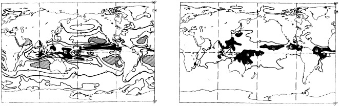
FIGURE 1
Mean (left) and standard deviation (right) of (E - P) from ECHAM3 T42 AGCM AMIP run.
White-White (WW) Atmospheric Model
At a given ocean-model grid point the anomalous freshwater flux for each time step was obtained from a set of normally distributed random numbers with zero mean and standard deviation of s mm/day. Values of s in the range 1 to 3 mm/day are approximately equal to the amplitude of the seasonal cycle of fresh-water flux that forces the OGCM. These values are also approximately equal to rms values obtained from the AMIP run, and to an independent estimate obtained by Roads et al. (1992) from the National Meteorological Center (NMC) analysis. The same procedure was used at each individual ocean-model grid point, so that the anomalous fresh-water flux that drove the OGCM had no spatial correlation in its covariance field and was uncorrelated in both space and time, i.e., white in both wave-number and frequency space. We refer to this as the white-white or WW model.
Red-White (RW) Atmospheric Model
The AMIP fresh-water flux anomaly field was represented as a series of empirical orthogonal functions (EOFs). The first 15 of these spatial functions en(x) and their associated eigenvalues ln were retained. At each time step of the OGCM, an anomalous global fresh-water flux field was constructed as the linear combination of products of the en(x) and n-random number with zero mean and standard deviation ln. This model had the spatial structure of the freshwater flux field from the T42, which was highly spatially correlated (red in wave-number space) while being random in time (white in frequency space). Note that each EOF mode carried the same variance, ln, as in the AMIP run. This type of stochastic atmospheric model is conceptually similar to but quantitatively different from that employed by MMR, and we refer to it here as the RW model.
Red-Red (RR) Atmospheric Model with Feedback
The AMIP data were used to develop a regression model relating the SST and SST gradients to the anomalous freshwater flux. The model used the 15 leading EOFs of the AMIP fresh-water flux and SST fields. The regression model was nearly global in nature, covering all ocean points where sea ice never occurred. In most regions it captured 80 to 90 percent of the variance in the original AMIP fresh-water flux data set (only 15 EOFs).5 However, the interesting fact was that the regression model captured a minimum of 96 percent of the variance associated with the first 15 EOFs. This result in turn suggests the highly linear relation between the SST and SST gradients and fresh-water flux. The basic approach to constructing such an atmospheric model can be found in Barnett et al. (1993).
Incorporation of the SST and SST gradient into the model obviously allows for a feedback between the ocean and pseudo-atmosphere and represents a type of coupled model not previously attempted on a global scale (although such a coupled model has produced good simulations of El Niño events (Barnett et al., 1993)). The relatively slow changes in SST ensure that the atmospheric model will be red in frequency space. The large-scale spatial correlations in both SST and fresh-water flux produce a wave-number dependence that is also red, so this model was called the red-red or RR model.
Experimental Setup
The basic model was run for 4000 years of simulated time forced only by the seasonal cycle. The state of the ocean at that time was taken as the initial condition for all subsequent runs. Four different basic simulations were
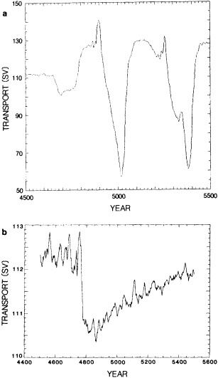
FIGURE 2
Transport (sverdrups) through the Drake Passage for OGCM forced by white-white noise (a) and red-white (b) noise.
carried out: The first was a continuation of the climatology run for an additional 1500 years. Results from this run have the designator C. Each of the three stochastic, anomalous fresh-water flux models was mated to the OGCM and run for 1500 years. The first 500 years of each integration were discarded, leaving the remaining 1000 years for analysis. The designators for these runs are WW, RW, or RR depending on which atmospheric model was used. All three anomaly runs included the same seasonal cycle, fresh-water flux, wind stress, and pseudo-heat flux forcing used in the climatology run.
RESULTS
This section briefly summarizes some of the more interesting results of the four experiments described above. Since this research effort is in the very early stages, these results are presented in descriptive form.
Antarctic Circumpolar Current Response
The model-simulated transport through the Drake Passage is shown in Figure 2 for several of the experiments. The C run shows nearly constant transport close to that observed, with annual variations of less than 1 percent (no illustration shown). The WW run, on the other hand, for s = 2 mm/day shows large variability, wherein the transport can change by 50 percent (Figure 2a). The time scale for this fluctuation is of the order of 300 years; it seems to be the mode of variation previously found by MMR (see below). By contrast, the RW run (Figure 2b) shows a step-like jump but otherwise low interdecadal variability. The feedback or RR run (not shown) is much like the RW run but with almost no high-frequency variability.
We deduced from the above results that the spatial correlation in the fresh-water forcing was not particularly important to the model response. Similarly, we concluded that it is the magnitude of the forcing in the high latitudes (only) that really affects the model behavior. We confirmed these conclusions by rerunning the RW case, but with the magnitude of the forcing increased by a factor of 5 for latitudes above 40°, where the RW atmospheric model was deficient in energy. This increased forcing brought the magnitude of the flux up to the order of I mm/day and corrected for the model's low variability in that region. The resulting transport through the Drake Passage (Figure 3) now resembles that found in the WW run with regard to both magnitude and time scale. In addition, similar experiments showed that it was the E - P flux south of 40°S that generated the MMR mode, while the flux in the northern ocean was of little significance other than local.
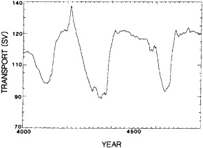
FIGURE 3
Same as red-white transport in Figure 2b, but run with variability above 40° latitude increased by a factor of 5.
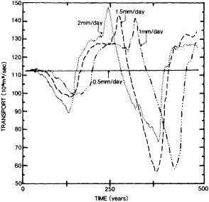
FIGURE 4
Drake Passage transport for white-white forcing with different levels of fresh-water flux variability. Atmospheric models and observation/analyses suggest that values of 1 to 2 mm/day are realistic in the higher-latitude regions.
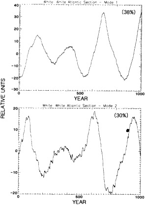
FIGURE 5
Principal components for Atlantic salinity section EOFs: white-white forcing.
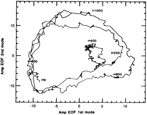
FIGURE 6
As in Figure 5, but for the Pacific section. The trajectory of the variability (the attractor) is shown in the phase space of the first two principal components.
The sensitivity of the Antarctic Circumpolar Current (ACC) transport to the magnitude of the forcing in the WW run was studied by repeating the experiment for values of s between 0.5 and 2.0 mm/day (Figure 4). The large-scale mode is excited rather uniformly by values above 1.0 mm/ day, but not by values of 0.5 mm/day or less (which resemble the control run). Note the similar shape of the responses in the range I to 2 mm, as well as a magnitude that is essentially independent of s. As the magnitude of the forcing is reduced, the mode takes longer to become excited. Apparently a threshold value between 0.5 to 1.0 mm is required to trigger the mode, and this fact suggests a highly nonlinear generation mechanism.
Meridional Structure
Salinity and temperature data from the WW run6 were saved along key meridional sections in both the Pacific and the Atlantic and subjected separately to EOF analysis. The principal components (PCs) for modes I and 2 for both oceans are shown in Figure 5 in standard format and in Figure 6 in two-dimensional phase space. It is clear that the roughly 300-year oscillation described above extends into the high latitudes of both major oceans. In the Atlantic, the PCs are in quadrature, and this means that the salinity anomalies propagate. The sense of the motion revealed by the EOFs (Figure 7) is that more (or less) saline water moves northward from Antarctica in the near-surface waters to the central North Atlantic where it sinks and returns at depth to the Southern Ocean. While this is happening, an
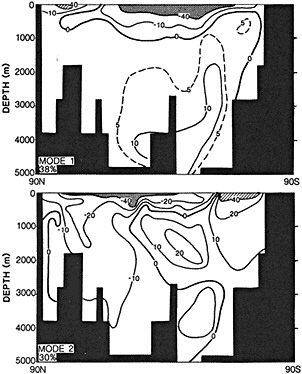
FIGURE 7
EOFs that accompany Figure 5.
anomaly of opposite sign is following the same trajectory, but 180° out of phase spatially. This is just the signal described by MMR, but it is produced here by totally white forcing as opposed to the RW forcing used in their experiment. As we saw above, the signal was also produced by our version of the RW forcing provided the magnitude of the high southern- latitude forcing was large enough.
The form of the signal in the Pacific (Figure 8) is somewhat like that found in the Atlantic. The two PCs form a rather simple attractor (Figure 6) and are in quadrature again, suggesting a propagating signal in the salinity field. The time scale is roughly 300 years, as found above. A major difference between the two oceans is that the signal does not penetrate in strength to the same depth it was found to in the Atlantic. The signal appears to propagate from one end of the ocean to the other, but is closely confined to the upper layers of the water column and has more spatial structure than in the Atlantic.
The simple correlation between the ACC transport fluctuations (Figure 2) and the variability of the salinity along the Atlantic-Pacific sections is shown in Figure 9. In the Atlantic, the plus-minus signature of the correlation field is indicative of the propagating signal discussed above. Note that major reductions in the strength of the ACC accompany reduced salinity over most of the South Atlantic to depths of the order of 1000 m. This is countered by increased salinity in the North Atlantic and in the deeper parts of the
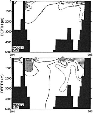
FIGURE 8
EOFs that accompany Figure 6.
entire Atlantic. The signature of the ACC variability in the Pacific is identical to that in the Atlantic, but only in the North Pacific. Most of the Pacific, even to the greatest depths, is more or less in phase with the ACC signal. However, the absolute values of the correlation in the Pacific are less than those found in the Atlantic.
Horizontal Structures
The horizontal structure of the low-frequency MMR signal is investigated in Figure 10, which shows the first and second EOFs of the Atlantic salinity anomaly at a depth of 700 m from the WW run. The associated PCs (not shown) suggest motion such that EOF1 leads EOF2. The first EOF shows the North and South Atlantic having anomalies of opposite sign. But note the negative anomaly extending into the Gulf of Mexico region. The second EOF shows the positive anomaly that occupied the North Atlantic has rotated and moved clockwise such that it is now off Africa. The negative anomaly has also moved clockwise so that it now covers most of the North Atlantic. These clockwise motions suggest that the anomalies are being influenced mainly by advection. Much the same type of anomaly motion is seen at 2000 m also.
The simple correlation between the ACC index and the salinity anomalies at 700 m and 2000 m is given in Figure 11. The entire Indian, North Pacific, and North Atlantic
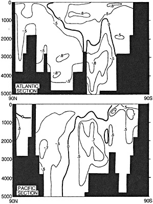
FIGURE 9
Correlation between Drake Passage transport and salinity variability along the meridional sections for the white-white forcing experiment.
oceans are in antiphase with the ACC at 700 m. Much the same pattern holds in these regions at 2000 m. The South Pacific and South Atlantic vary in phase with the ACC at both depths, but an unexpectedly strong signal (positive) is apparent in the western Equatorial Pacific. At 700 m the strongest signals are in the Indian Ocean, but at 2000 m this distinction is held by the South Pacific and the North Atlantic. It is obvious that the ocean mode of variation discussed here is truly global in extent.
Levels of Variability
The rms variability of the salinity field from the WW and RR runs is shown in Figure 12 for depths of 75 m. The RR run produces far more variance in the salinity field, especially in the deep ocean (e.g., 2000 m, not shown) where rms values of 0.06 to 0.08 psu are common in higher latitudes. The spatial distribution of the variability between the two runs clearly shows the importance of large-scale air-sea interactions in forcing the model. If the RR run is at all realistic, then the coupling between the two media needs to be taken into account in studies of interdecadal variability. It is interesting that the spatial structure of the
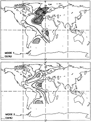
FIGURE 10
Leading EOFs of Atlantic salinity field at 700 m from the white-white run.
modal response was similar between all the runs, even if the levels of variance were not. This suggests the response is a leading "eigenmode" of the global ocean model that is easily excited by a wide range of forcing.
SUMMARY
A reasonably sophisticated, realistic OGCM has been forced with annual cycles of wind stress, temperature, and fresh-water flux, and also with anomalies of fresh-water flux. The latter anomaly model simulations range from forcing that is white in both space and time to a model that is red in both domains and also incorporates feedback between the fresh-water flux and local SST.
The results of these simulations show a richly structured response. One prominent mode is that discovered by Mikolajewicz and Maier-Reimer (1990, 1991). We found that mode is driven principally by anomalous fresh-water flux in the higher latitudes of the Southern Hemisphere. The spatial structure and details of the forcing are not as important to the mode as the magnitude of the forcing. Monthly anomalies greater than 1 mm/day will excite the mode, while values below 0.5 mm/day do not. Atmospheric-model results and NMC analyses suggest that realistic values of anomalous fresh-water flux in the high latitudes are of the order
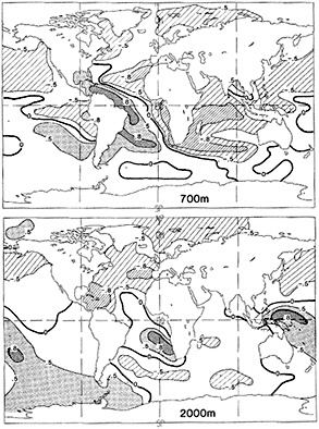
FIGURE 11
Correlation between Drake Passage transport and salinity variations at 700 m and 2000 m for the 1000 year white-white run.
of 1 to 2 mm/day, so the forcing required for this mode in the OGCM may not be unrealistic.
The principal mode referred to above has expressions in all major oceans, and is also associated with changes in the transport of the ACC by a factor of two. The mode in the Atlantic is associated with a meridional overturning of the entire ocean and a horizontal circulation that is clockwise. The mode in the Pacific does not penetrate in strength as deeply as in the Atlantic, and it appears to have a more difficult time extending across the equator.
The levels of interdecadal variability produced by the model for virtually all of the atmospheric forcing models we used was surprisingly large in view of the coarse OGCM resolution. If these levels of variance were found in the
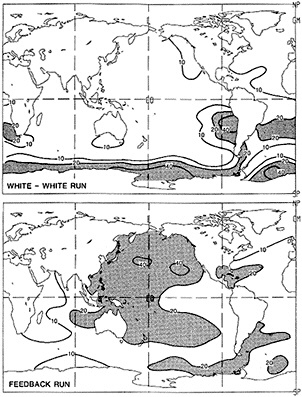
FIGURE 12
Standard deviation of salinity (psu) at 75 m from two noise-forced runs.
real-world ocean, they would represent an important level of change.
ACKNOWLEDGMENTS
This work was supported by the Department of Energy through its Computer Hardware, Advanced Mathematics, and Model Physics (CHAMMP) effort under contract DE-FG03-91-ER61215, and by the National Science Foundation under Grant NSF ATM88-14571-03. The Deutsche Forschungsgemeinschaft and the Sonderforschungbereich 318 provided support for U. Mikolajewicz. M. Schultz helped with the drafting and T. Tubbs carried through many of the key computations. R. Wilde was supported under the NSF program for undergraduate research (REU).
Commentary on the Paper of Barnett et al.
KEVIN E. TRENBERTH
National Center for Atmospheric Research
Dr. Barnett has given us a very "colorful" talk dealing with an ocean GCM that has very simple forcing. The nature of the forcing, as he mentioned, is critical in terms of its magnitude in particular, and its special character to a lesser degree. The first thing that I thought of—probably a minor point—with regard to the fresh-water forcing is the aspect dealing with runoff from rivers into the ocean. In fact, the precipitation exceeds evaporation over land in general. Is that in the model? If you just model E - P over the ocean, there will be imbalances, because there E exceeds P. What does that do to the overall fresh-water balance?
Dr. Barnett used three kinds of forcings. The main one he talked about was the white/white, which seems somewhat unrealistic. He used a global standard deviation value of 2 mm/day. That number may be reasonable globally, but should be much larger than that in the tropics and about half that in high latitudes. But large numbers at high latitudes were one of the critical things in getting this oscillation.
My other concern is that I consider the model to be unnaturally constrained. Any time you use an idealized atmosphere, the nature of the fluxes into the model ocean and the ability of the atmosphere to feed back and adjust in various ways are limited. For instance, can the climate system adjust to compensate for the fresh-water flux? The parameterization derived here for the red/red case, especially in the tropics, does indicate that the fresh-water flux can be altered substantially by changes in sea temperatures. Certainly other aspects of land-ocean differences introduce similar complexities. Therefore, the relevance of something like this to the real world is, I think, a very open question.
Dr. Barnett did not talk about mechanisms, although maybe other atmospheric modelers will. Perhaps, because the model integrations are made over wide areas, the spatial structure does not matter much; if the area mean is the main thing that counts, the result is a red spectrum whatever you do. Wide-area integration also implies that there is a random-walk process that will result in perturbations in the fresh-water flux. The perturbations will affect or even shut down the thermohaline circulation, which will alter the heat balance because of the heat transports involved, which in turn will cause changes in temperatures.
This process is reflected in the temperature variations the model exhibits at high latitudes. Dr. Barnett asks, "Is this natural variability something that is going to confound us when we look at the greenhouse effect?" But ultimately, shutting down the thermohaline circulation will change the temperatures enough that they will probably cause the thermohaline circulation to jerk back into action at some point and advect fresh-water around. Might this be part of the mechanism that results in an oscillation? I do not know. I think the bottom line is the question of these models' relevance to the real world.
Discussion
BARNETT: That last question does need to be kept in mind, but for a full-ocean GCM our model does quite a good job of reproducing the main features of the global ocean.
TRENBERTH: Isn't the forcing at high latitudes much higher than in the AMIP run?
BARNETT: Not much. We picked 2 mm/day because it's a fairly good global average, and I think it's fairly realistic. I believe some other models using a smaller figure still get the oscillation.
SARACHIK: Why did you choose to show the transport of the Antarctic circumpolar current, and what was the structure of the changes in it?
BARNETT: It's a simple diagnostic for the system. If you have no signal there, you won't have much anywhere.
BRYAN: I'd like to respond to Kevin's comment about runoff. For the North Atlantic, I believe that runoff is dominant at very high latitudes simply because the coastline is so extensive by comparison with the ocean area. If you also take into account the tremendous Arctic fresh-water discharge, the total runoff is much greater than the local net precipitation.
BARNETT: This runoff effect has been included in a couple of models for the Hamburg greenhouse runs, and it's my impression that it didn't make much difference. If it is large, though, it should be fairly simple to put into these kinds of models.
TRENBERTH: Runoff might affect the nature of feedbacks, and clearly on time scales that cover the melting of major ice caps it would become critical.
WEAVER: It seems to me that you do have a sort of parameteriza-
tion of the runoff, since you obtain your mean fresh-water flux from diagnosing a spun-up state that you got from observed salinities.
MYSAK: Have you done any sensitivity studies for your model's parameters?
BARNETT: No, though others have. It's tuned to today's climate. I don't think it's particularly diffusive, for instance.
MYSAK: One of the things we were interested in doing with the very simple two-dimensional thermohaline model was the Maier-Reimer experiment. We looked at its sensitivity to diffusivities, for example, to see just how robust the 200-to-300-year oscillation was. We found that it was fairly robust over a fairly wide range, and very robust for a certain set of parameters. For the extreme of a very diffusive ocean, the 200-year oscillation was damped out, and the system alternated between sinking in the north and sinking in the south.
LEHMAN: I have two questions. What is the sensitivity of this model to fresh-water forcing? Convection in the model Maier-Reimer used collapsed with a .02-sverdrup increase to the northern part of the North Atlantic. Second, do you know why the model is more sensitive to Southern Hemisphere forcing than Northern?
TRENBERTH: It might simply be the respective sizes of the oceans. If you're doing random forcing that has no spatial structure, you need a large area to integrate over to get a decent-sized signal.
BARNETT: The odd thing is that you get about the same answer when you use white noise as when you use something with nice big spatial scales.
YOUNG: Have you thought about computing the gain by calculating the linear eigenmodes?
BARNETT: I believe we've done that numerically by forcing it with white noise. The transfer function of the model is essentially the empirical orthogonal function. But we've barely begun to look at it.
MARTINSON: The fluctuations that come out of these models are very interesting. Of course it's hard to equate them with reality when some of the regions appear to be so sensitive that you could spit off a ship and cause the ice cover to disappear. I think in most cases there is a whole set of self-regulating feedbacks that prevent the system from overturning like that. I'd like to get some of us together to look at the fine-scale local processes in terms of your larger-scale results and see whether indeed your model is representative in what you might call a budget sense.
BARNETT: I'd be glad to join you. We did manage to take sea ice into account and not destroy it too badly—though our answers weren't very different from those of models without any—but we really don't know how well the integral properties represented by this model resemble reality.
MYSAK: My feeling is that on the 200-to-300-year time scale the sea ice is probably not going to influence the results.
TRENBERTH: Ah, but having ice in the model allows for many other feedbacks to the atmosphere that make the system even more complex.
Ocean Modeling Reference List
Andrews, D.G., and M.E. McIntyre. 1976. Planetary waves in horizontal and vertical shear: The generalized Eliassen-Palm relation and the mean zonal acceleration. J. Atmos. Sci. 33:2031-2048.
Armi, L. 1978. Some evidence for boundary mixing in the deep ocean. J. Geophys. Res. 83:1971-1979.
Barnett, T.P., N. Graham, M. Latif, S. Pazan, and W. White. 1993. ENSO and ENSO-related predictability. Part 1: Prediction of equatorial Pacific sea surface temperature with a hybrid coupled ocean-atmosphere model. J. Climate 6:1545-1566.
Barnett, T.P., M. Chu, R. Wilde, U. Mikolajewicz. 1995. Low-frequency ocean variability induced by stochastic forcing of various colors. In Natural Climate Variability on Decade-to-Century Time Scales. D.G. Martinson, K. Bryan, M. Ghil, M.M. Hall, T.R. Karl, E.S. Sarachik, S. Sorooshian, and L.D. Talley, eds. National Academy Press, Washington, D.C.
Batchelor, G. 1969. Computation of the energy spectrum in homogeneous, two-dimensional turbulence. Phys. Fluids 12:233-238.
Baumgartner, A., and E. Reichel. 1975. The World Water Balance. Elsevier, New York.
Birchfield, G.E., H. Wang, and M. Wyant. 1990. A bimodal climate response controlled by water vapor transport in a coupled ocean-atmosphere box model. Paleoceanography 5:383-395.
Bjerknes, J. 1964. Atlantic air-sea interaction. Adv. Geophys. 10:1-82.
Bjerknes, J. 1969. Atmospheric telecommunications from the equatorial Pacific. Mon. Weather Rev. 97:163-172.
Boyle, E.A., and L.D. Keigwin. 1987. North Atlantic thermohaline circulation during the past 20,000 years linked to high-latitude surface temperature. Nature 330:35-40.
Bretherton, F.P. 1982. Ocean climate modeling. Prog. Oceanogr. 11:93-129.
Bretherton, F., and D. Haidvogel. 1976. Two-dimensional turbulence above topography. J. Fluid Mech. 78:129-154.
Briegleb, B.P. 1991. Description of CCM2 Radiative/Convective Model. Climate Modeling Section Note No. 4, National Center for Atmospheric Research, Boulder, Colo.. 11 pp.
Broecker, W.S. 1989. The salinity contrast between the Atlantic and Pacific Oceans during glacial time. Paleoceanography 4:207-212.
Broecker, W.S., D.M. Peteet, and D. Rind. 1985. Does the ocean-atmosphere system have more than one stable mode of operation? Nature 315:21-26.
Broecker, W.S., G. Bond, and M. Klas. 1990. A salt oscillator in the glacial Atlantic? 1. The concept. Paleoceanography 5:469-477.
Bryan, F. 1986a. Maintenance and Variability of the Thermohaline Circulation. Ph.D. dissertation, Princeton University, 254 pp.
Bryan, F. 1986b. High latitude salinity effects and interhemispheric thermohaline circulations. Nature 323:301-304.
Bryan, F. 1986c. Parameter sensitivity of primitive equation ocean general circulation models. J. Phys. Oceanogr. 17:970-985.
Bryan, K. 1969. A numerical method for the study of the circulation of the World Ocean. J. Comput. Phys. 3:347-376.
Bryan, K. 1979. Models of the world ocean. Dyn. Atmos. Oceans 3:327-338.
Bryan, K. 1984. Accelerating the convergence to equilibrium of ocean climate models. J. Phys. Oceanogr. 14:666-673.
Bryan, K., and M.D. Cox. 1972. An approximate equation of state for numerical models of ocean circulation. J. Phys. Oceanogr. 2:510-517.
Bryan, K., and F.C. Hansen. 1995. A toy model of North Atlantic climate variability on a decade-to-century time scale. In Natural Climate Variability on Decade-to-Century Time Scales. D.G. Martinson, K. Bryan, M. Ghil, M.M. Hall, T.R. Karl, E.S. Sarachik, S. Sorooshian, and L.D. Talley. eds. National Academy Press, Washington, D.C.
Bryan, K., and J.L. Lewis. 1979. A water mass model of the world ocean. J. Geophys. Res. 84:2503-2517.
Bryan, K., and R. Stouffer. 1991. A note on Bjerknes' hypothesis for North Atlantic variability. J. Mar. Systs. 1:229-241.
Cai, W., and S.J. Godfrey. 1995. Surface heat flux parameterizations and the variability of thermohaline circulation. J. Geophys. Res. 100:10679-10692.
Cattle, H.. 1985. Diverting Soviet rivers: Some possible repercussions for the Arctic Ocean. Polar Record 22:485-498.
Charney, J. 1971. Geostrophic turbulence. J. Atmos. Sci. 28:1087-1095.
Cook, E.R., B.M. Buckley, and R.D. D'Arrigo. 1995. Interdecadal temperature oscillations in the Southern Hemisphere: Evidence from Tasmanian tree rings since 300 B.C. In Natural Climate Variability on Decade-to-Century Time Scales. D.G. Martinson, K. Bryan, M. Ghil, M.M. Hall, T.R. Karl, E.S. Sarachik, S. Sorooshian, and L.D. Talley (eds.). National Academy Press, Washington, D.C.
Cox, M. 1987. Isopycnal diffusion in a z-coordinate ocean model. Ocean Model. 74:1-5.
Cox, M.D. 1984. A Primitive Equation, Three Dimensional Model of the Ocean. GFDL Ocean Group Technical Report No. 1, NOAA, 143 pp.
Dansgaard, W., S.J. Johnsen, H.B. Clausen, and C.C. Langway. 1970. Climatic record revealed by the Camp Century ice core. In The Late Cenozoic Glacial Ages. K.K. Turekian (ed.). Yale University Press, pp. 37-56.
Dansgaard, W., J.W.C. White, and S.J. Johnsen. 1989. The abrupt termination of the Younger Dryas climate event. Nature 339:532-534.
Deardorff, J.W. 1972. Theoretical expression for the counter-gradient vertical heat flux. J. Geophys. Res. 77:5900-5904.
Delworth, T., S. Manabe, and R.J. Stouffer. 1993. Interdecadal variability of the thermohaline circulation in a coupled ocean-atmosphere model. J. Climate 6:1993-2011.
Delworth, T., S. Manabe, and R. Stouffer. 1995. North Atlantic interdecadal variability in a coupled model. In Natural Climate Variability on Decade-to-Century Time Scales. D.G. Martinson, K. Bryan, M. Ghil, M.M. Hall, T.R. Karl, E.S. Sarachik, S. Sorooshian, and L.D. Talley (eds.). National Academy Press, Washington, D.C.
Dickson, R.R., J. Meincke, S.-A. Malmberg, and A.J. Lee. 1988. The Great Salinity Anomaly in the northern North Atlantic 1968-1982. Prog. Oceanogr. 20:103-151.
Dietrich, G., and J. Ulrich. 1968. Atlas zur Ozeanographie. Bibliogr. Institut, Mannheim, 79 pp.
Duplessy, J.C., N.J. Shackleton, R.G. Fairbanks, L. Labeyrie, D. Oppo, and N. Kallel. 1988. Deepwater source variations during the last climate cycle and their impact on the global deepwater circulation. Paleoceanography 3:343-360.
Flato, G.M., and W.D. Hibler. 1990. On a simple sea-ice dynamics model for climate studies. Ann. Glaciol. 14:72-77.
Folland, C.K., D.E. Parker, M.N. Ward, and A.W. Colman. 1986. Sahel rainfall, northern hemisphere circulation anomalies and worldwide temperature changes . Long Range Forecasting and Climate Research, Memorandum #7a. Meteorological Office, Bracknell, U.K., 49 pp.
Gargett, A., and G. Holloway. 1984. Dissipation and diffusion by internal wave breaking. J. Mar. Res. 42:15-27.
Garrett, C. 1991. Marginal mixing theories. Atmos.-Ocean 29:313-339.
Garwood, R.W. 1977. An oceanic mixed-layer model capable of simulating cyclic states. J. Phys. Oceanogr. 7:446-468.
Gaspar, P. 1988. Modeling the seasonal cycle of the upper ocean. J. Phys. Oceanogr. 18:161-180.
Gent, P.R., and J.C. McWilliams. 1990. Isopycnal mixing in ocean models. J. Phys. Oceanogr. 20:150-155.
Ghil, M., and R. Vautard. 1991. Interdecadal oscillations and the warming trend in global temperature time series. Nature 350:324-327.
Ghil, M., A. Mullhaupt, and P. Pestiaux. 1987. Deep water formation and Quaternary glaciations . Climate Dynamics 2:1-10.
Gray, W.M. 1990. Strong association between West African rainfall and U.S. landfall of intense hurricanes. Science 249:1251-1256.
Greatbatch, R.J., and S. Zhang. 1995. An interdecadal oscillation in an idealized ocean basin forced by constant heat flux. J. Climate 8:81-91.
Greatbatch, R.J., A.F. Fanning, A.D. Goulding, and S. Levitus. 1991. A diagnosis of interpentadal circulation changes in the North Atlantic. J. Geophys. Res. 96:22009-22023.
Gregg, M. 1987. Dyapycnal mixing in the thermocline: A review. J. Geophys. Res. 92:5249-5286.
Haney, R.L. 1971. Surface thermal boundary condition for ocean circulation models. J. Phys. Oceanogr. 1:241-248.
Hansen, J., and S. Lebedeff. 1987. Global trends of measured surface air temperature. J. Geophys. Res. 92:13345-13374.
Hasselmann, K. 1976. Stochastic climate models. Part I. Theory. Tellus 28:289-305.
Hellerman, S., and M. Rosenstein. 1983. Normal monthly wind stress over the world ocean with error estimates. J. Phys. Oceanogr. 13:1093-1104.
Hibler, W.D. 1979. A dynamic thermodynamic sea ice model. J. Phys. Oceanogr. 9:815-846.
Hibler, W.D., and S.J. Johnsen. 1979. The 20-year cycle in Greenland ice core records. Nature 280:481-483.
Holloway, G. 1978. A spectral theory of nonlinear barotropic motion above irregular topography. J. Phys. Oceanogr. 8:414-427.
Holloway, G. 1987. Systematic forcing of large-scale geostrophic flows by eddy-topography interaction. J. Fluid Mech. 184:463-476.
Holloway, G. 1992. Representing topographic stress for large-scale ocean models. J. Phys. Oceanogr. 22:1033-1046.
Holtslag, A.A.M., and C.-H. Moeng. 1991. Eddy diffusivity and countergradient transport in the convective atmospheric boundary layer. J. Atmos. Sci. 48:1690-1698.
Huang, R.X., J.R. Luyten, and H.M. Stommel. 1992. Multiple equilibrium states in a combined thermal and saline circulation. J. Phys. Oceanogr. 22:231-246.
Hughes, T.M.C., and A.J. Weaver. 1994. Multiple equilibria of an asymmetric two-basin ocean model. J. Phys. Oceanogr. 24:619-637.
Ikeda, M. 1990. Decadal oscillations of the air-ice-ocean system in the northern hemisphere. Atmos.-Ocean 28:106-139.
IPCC. 1990. Climate Change: The IPCC Scientific Assessment. J.T. Houghton, G.J. Jenkins, and J.J. Ephraums (eds.). Prepared
for the Intergovernmental Panel on Climate Change by Working Group I. WMO/UNEP, Cambridge Univ. Press, 365 pp.
Iselin, C. 1939. The influence of vertical and lateral turbulence on the characteristics of the waters at mid-depths. Eos, Trans. AGU 20:414-417.
Keeling, C.D., and T.P. Whorf. 1995. Decadal oscillations in global temperature and atmospheric carbon dioxide. In Natural Climate Variability on Decade-to-Century Time Scales. D.G. Martinson, K. Bryan, M. Ghil, M.M. Hall, T.R. Karl, E.S. Sarachik, S. Sorooshian, and L.D. Talley (eds.). National Academy Press, Washington, D.C.
Keigwin, L.A., G.A. Jones, and S.J. Lehman. 1991. Deglacial meltwater discharge, North Atlantic deep circulation and abrupt climate change. J. Geophys. Res. 96:16811-16826.
Kleeman, R., and S.B. Power. 1995. A simple atmospheric model of surface heat flux for use in ocean modeling studies. J. Phys. Oceanogr. 25:92-105.
Krishnamurti, T.N., S.-H. Chu, and W. Iglesias. 1986. On the sea level pressure of the southern oscillation. Arch. Meteor. Geophys. Bioklimatol., Series A, 34:385-425.
Kushnir, Y. 1994. Interdecadal variations in North Atlantic sea surface temperature and associated atmospheric conditions. J. Climate 7:141-157.
Labeyrie, L.D., J.C. Duplessy, and P.L. Blanc. 1987. Variations in mode of formation and temperature of oceanic deep waters over the past 125,000 years. Nature 327:477-482.
Large, W.G., J.C. McWilliams, and S.C. Doney. 1994. Oceanic vertical mixing: A review and a model with a non-local K-profile boundary layer parameterization . Rev. Geophys. 32:363-403.
Lazier, J.R.N. 1980. Oceanographic conditions at Ocean Weather Ship BRAVO, 1944-1974. Atmos.-Ocean 18:227-238.
LeBlond, P.H., and L.A. Mysak. 1978. Waves in the Ocean. Elsevier, Amsterdam, 602 pp.
Lemke, P., W.B. Owens, and W.D. Hibler. 1990. A coupled sea ice-mixed layer-pycnocline model for the Weddell Sea. J. Geophys. Res. 95:9513-9525.
Levitus, S. 1982. Climatological Atlas of the World Ocean. NOAA Professional Paper 13, U.S. Department of Commerce: National Oceanic and Atmospheric Administration, Washington, D.C., 173 pp. + 17 microfiches.
Levitus, S. 1989a. Interpentadal variability of temperature and salinity at intermediate depths of the North Atlantic Ocean, 1970-74 versus 1955-59. J. Geophys. Res. 94:6091-6131.
Levitus, S. 1989b. Interpentadal variability of salinity in the upper 150 m of the North Atlantic Ocean, 1970-74 versus 1955-59. J. Geophys. Res. 94:9679-9685.
Levitus, S. 1989c. Interpentadal variability of temperature and salinity in the deep North Atlantic, 1970-74 versus 1955-59. J. Geophys. Res. 94:16125-16131.
Levitus, S. 1990. Interpentadal variability of steric sea level and geopotential thickness of the North Atlantic Ocean, 1970-74 versus 1955-59. J. Geophys. Res. 95:5233-5238.
Loder, J.W., and C. Garrett. 1978. The 18.6-year cycle of sea surface temperature in shallow seas due to variations in tidal mixing. J. Geophys. Res. 83:1967-1970.
Lumley, J.A., and H.A. Panofsky. 1964. The Structure of Atmospheric Turbulence. John Wiley and Sons, New York City, 239 pp.
Maier-Reimer, E., U. Mikolajewicz, and K. Hasselmann. 1993. Mean circulation of the Hamburg LSG OGCM and its sensitivity to the thermohaline surface forcing. J. Phys. Oceanogr. 23:731-757.
Manabe, S., and R.J. Stouffer. 1988. Two stable equilibria of a coupled ocean-atmosphere model. J. Climate 1:841-866.
Marotzke, J. 1989. Instabilities and multiple steady states of the thermohaline circulation. In Oceanic Circulation Models: Combining Data and Dynamics. D.L.T. Anderson and J. Willebrand (eds.). NATO ASI series, Kluwer, Dordrecht, pp. 501-511.
Marotzke, J. 1990. Instabilities and multiple equilibria of the thermohaline circulation. Ph.D. Dissertation, Ber. Institut für Meereskunde, Kiel, 126 pp.
Marotzke, J. 1991. Influence of convective adjustment on the stability of the thermohaline circulation. J. Phys. Oceanogr. 21:903-907.
Marotzke, J., and P.H. Stone. 1995. Atmospheric transports, the thermohaline circulation, and flux adjustments in a simple coupled model. J. Phys. Oceanogr. 25:1350-1364.
Marotzke, J., and J. Willebrand. 1991. Multiple equilibria of the global thermohaline circulation. J. Phys. Oceanogr. 21:1372-1385.
Marotzke, J., P. Welander, and J. Willebrand. 1988. Instability and multiple steady states in a meridional-plane model of the thermohaline circulation. Tellus 40A: 162-172.
Marshall, J. 1981. On the parameterization of geostrophic eddies in the ocean. J. Phys. Oceanogr. 11:257-271.
Martin, P.J. 1985. Simulation of the mixed layer at OWS November and Papa with several models. J. Geophys. Res. 90:903-916.
McCready, P., and P. Rhines. 1991. Buoyant inhibition of Ekman transport on a slope and its effect on stratified spin-up. J. Fluid Mech. 223:631-661.
McDermott, D., and E.S. Sarachik. 1995. Thermohaline circulations and variability in a two-hemisphere sector model of the Atlantic. In Natural Climate Variability on Decade-to-Century Time Scales. D.G. Martinson, K. Bryan, M. Ghil, M.M. Hall, T.R. Karl, E.S. Sarachik, S. Sorooshian, and L.D. Talley, eds. National Academy Press, Washington, D.C.
McWilliams, J. 1984. The emergence of isolated coherent vortices in turbulent flow. J. Fluid Mech. 146:21-43.
McWilliams, J. 1985. Sub-mesoscale coherent vortices in the ocean. Rev. Geophys. 23:165-182.
McWilliams, J. 1989. Statistical properties of decaying geostrophic turbulence. J. Fluid Mech. 198:199-230.
McWilliams, J.C. 1995. Sub-grid-scale parameterization in ocean general-circulation models. In Natural Climate Variability on Decade-to-Century Time Scales. D.G. Martinson, K. Bryan, M. Ghil, M.M. Hall, T.R. Karl, E.S. Sarachik, S. Sorooshian, and L.D. Talley, eds. National Academy Press, Washington, D.C.
McWilliams, J.C., and J.H.S. Chow. 1981. Equilibrium geostrophic turbulence: A reference solution in a ß-plane channel. J. Phys. Oceanogr. 11:921-949.
McWilliams, J.C, and P.R. Gent. 1994. The wind-driven ocean circulation with an isopycnal-thickness mixing parameterization. J. Phys. Oceanogr. 24:46-65.
McWilliams, J.C., W.R. Holland, and J.H.S. Chow. 1978. A description of numerical Antarctic circumpolar currents. Dyn. Atmos. Oceans 2:213-291.
McWilliams, J., and 20 co-authors. 1983. The local dynamics of eddies in the western North Atlantic. In Eddies in Marine Science. A. Robinson (ed.). Springer-Verlag, Berlin, pp. 92-113.
McWilliams, J.C., P.C. Gallacher, C.-H. Moeng, and J.C. Wyngaard. 1993. Modeling the oceanic planetary boundary layer. In Large Eddy Simulation of Complex Engineering and Geophysical Flows. B. Galperin and S. Orszag (eds.). Lecture Notes in Engineering, Cambridge University Press, pp. 441-454.
Mellor, G.L., and T. Yamada. 1982. Development of a turbulence closure model for geophysical fluid dynamics. Rev. Geophys. Space Phys. 20:851-875.
Mikolajewicz, U., and E. Maier-Reimer. 1990. Internal secular variability in an ocean general circulation model. Climate Dynamics 4:145-156.
Mikolajewicz, U., and E. Maier-Reimer. 1991. One example of a natural mode of the ocean circulation in a stochastically forced ocean general circulation model. In Strategies for Future Climate Research. M. Latif (ed.). Available from Max Planck-Institut für Meteorologie, Hamburg, Germany, pp. 287-318.
Milliff, R.A., and J.C. McWilliams. 1994. The evolution of boundary pressure in enclosed ocean basins. J. Phys. Oceanogr. 24:1317-1338.
Montgomery, R. 1940. The present evidence on the importance of lateral mixing processes in the ocean. Bull. Am. Meteorol. Soc. 21:87-94.
Moore, A.M., and C.J.C. Reason. 1993. The response of a global ocean general circulation model to climatological surface boundary conditions for temperature and salinity. J. Phys. Oceanogr. 23:300-328.
Myers, P.G., and A.J. Weaver. 1992. Low-frequency internal oceanic variability under seasonal forcing. J. Geophys. Res. 97:9541-9563.
Mysak, L.A., and D.K. Manak. 1989. Arctic sea-ice extent and anomalies, 1953-1984. Atmos.-Ocean 27:376-405.
Mysak, L.A., D.K. Manak, and R.F. Marsden. 1990. Sea-ice anomalies in the Greenland and Labrador Seas during 1901-1984 and their relation to an interdecadal Arctic climate cycle. Climate Dynamics 5:111-133.
Mysak, L.A., T.F. Stocker, and F. Huang. 1993. Century-scale variability in a randomly forced, two-dimensional thermohaline ocean circulation model. Climate Dynamics 8:103-116.
O'Brien, J.J. 1970. A note on the vertical structure of the eddy exchange coefficient in the planetary boundary layer. J. Atmos. Sci. 27:1213-1215.
Oeschger, H., J. Beer, U., Siegenthaler, and B. Stauffer. 1984. Late-glacial climate history from ice cores. In Climate Processes and Climate Sensitivity . J.E. Hansen and T. Takahashi (eds.). Geophysical Monographs 29, Maurice Ewing Volume 5, American Geophysical Union, Washington, D.C., pp. 299-306.
Pacanowski, R., and G. Philander. 1981. Parameterization of vertical mixing in numerical models of tropical oceans. J. Phys. Oceanogr. 11:1443-1451.
Peters, H., M. Gregg, and J. Toole. 1988. On the parameterization of equatorial turbulence. J. Geophys. Res. 93:1199-1218.
Pierce, D.W., T.P. Barnett, and U. Mikolajewicz. Unpublished manuscript, 1994. On the competing roles of heat and fresh-water flux in forcing thermohaline oscillations.
Quon, C., and M. Ghil. 1992. Multiple equilibria in thermosolutal convection due to salt-flux boundary conditions. J. Fluid Mech. 235:449-483.
Rahmstorf, S., and J. Willebrand. 1995. The role of temperature feedback in stabilizing the thermohaline circulation. J. Phys. Oceanogr. 25:787-805.
Redi, H. 1982. Oceanic isopycnal mixing by coordinate rotation. J. Phys. Oceanogr. 12:1154-1158.
Rhines, P.B., and W.R. Young. 1982. Homogenization of potential vorticity in planetary gyres. J. Fluid Mech. 122:347-367.
Roads, J.O., S.-C. Chen, J. Kao, D. Langley, and G. Glatzmaier. 1992. Global aspects of the Los Alamos general circulation model hydrologic cycle. J. Geophys. Res. 97(D9):10051-10068.
Roeckner, E., K. Arpe, L. Bengtsson, S. Brinkop, L. Dumenil, M. Esch, E. Kirk, F. Lunkeit, M. Ponater, B. Rockel, R. Sausen, U. Schlese, S. Schubert, and M. Windelband. 1992. Simulation of the present-day climate with the ECHAM model: Impact of model physics and resolution. Rept. No. 93, Max Planck-Institut für Meteorologie, Hamburg.
Roemmich, D., and C. Wunsch. 1984. Apparent changes in the climatic state of the deep North Atlantic Ocean. Nature 307:447-450.
Roemmich, D., and C. Wunsch. 1985. Two transatlantic sections: Meridional circulation and heat flux in the subtropical North Atlantic Ocean. Deep-Sea Res. 32:619-664.
Ruddiman, W., and A. McIntyre. 1977. Late Quaternary surface ocean kinematics and climate change in the high-latitude North Atlantic. J. Geophys. Res. 82:3877-3887.
Sarmiento, J.L., R.D. Slater, M.J.R. Fasham, H.W. Ducklow, J.R. Toggweiler, and G.T. Evans. 1993. A seasonal three-dimensional ecosystem model of nitrogen cycling in the North Atlantic euphotic zone. Glob. Biogeochem. Cycl. 7:415-450.
Schlosser, P., G. Bönisch, M. Rhein, and R. Bayer. 1991. Reduction of deepwater formation in the Greenland Sea during the 1980s: Evidence from tracer data. Science 251:1054-1056.
Schmitt, R.W., P.S. Bogden, and C.E. Dorman. 1989. Evaporation minus precipitation and density fluxes for the North Atlantic. J. Phys. Oceanogr. 19:1208-1221.
Schopf, P.S. 1985. Modeling tropical sea-surface temperature: Implications of various atmospheric responses. In Coupled Ocean-Atmosphere Models. J. Nihoul (ed.). Elsevier Oceanography Series No. 40, Amsterdam, pp. 727-734.
Spall, M.A. 1992. Variability of sea surface salinity in stochastically forced systems. Climate Dynamics 8:151-160.
Stocker, T.F. and L.A. Mysak. 1992. Climatic fluctuations on the century time scale: A review of high-resolution proxy data and possible mechanisms. Climate Change 20:227-250.
Stommel, H. 1961. Thermohaline convection with two stable regimes of flow. Tellus 13:224-230.
Sverdrup, H.U. 1957. Oceanography. In Handbuch der Physik. Springer-Verlag, Berlin, 48:630-638.
Tennekes, H. 1973. A model for the dynamics of the inversion above a convective boundary layer. J. Atmos. Sci. 30:558-567.
Toggweiler, J.R., and B. Samuels. 1992. Is the magnitude of the deep outflow from the Atlantic Ocean actually governed by the Southern Hemisphere winds? In The Global Carbon Cycle. M. Heimann (ed.). NATO ASI Series, Springer-Verlag, Berlin, pp. 303-331.
Toggweiler, J.R., K. Dixon, and K. Bryan. 1989. Simulations of radiocarbon in a coarse-resolution world ocean model. I: Steady state, pre-bomb distributions. J. Geophys. Res. 94:8217-8242.
Treguier, A. 1989. Topographically generated steady currents in barotropic turbulence. Geophys. Astrophys. Fluid Dyn. 47:43-68.
Treguier, A., and J. McWilliams. 1990. Topographic influences on wind-driven, stratified flow in a ß-plane channel: An idealized model for the Antarctic Circumpolar Current models. J. Phys. Oceanogr. 20:321-343.
Trenberth, K.E., W.G. Large, and J.G. Olson. 1990. The mean annual cycle in global ocean wind stress. J. Phys. Oceanogr. 20:1742-1760.
Troen, I.B., and L. Mahrt. 1986. A simple model of the atmospheric boundary layer: Sensitivity to surface evaporation. Bound.-Layer Meteorol. 37:129-148.
UNESCO. 1981. Tenth report of the Joint Panel on Oceanographic Tables and Standards. UNESCO Technical Paper on Marine Science No. 36, UNESCO, Paris.
Walin, G. 1985. The thermohaline circulation and control of ice ages. Paleogr. Paleoclim. Paleoecol. 50:323-332.
Weaver, A.J. 1995. Decadal-to-millennial internal oceanic variability in coarse-resolution ocean general-circulation models . In Natural Climate Variability on Decade-to-Century Time Scales. D.G. Martinson, K. Bryan, M. Ghil, M.M. Hall, T.R. Karl, E.S. Sarachik, S. Sorooshian, and L.D. Talley, eds. National Academy Press, Washington, D.C.
Weaver, A.J., and T.M.C. Hughes. 1992. Stability and variability of the thermohaline circulation and its link to climate. In Trends in Physical Oceanography. No. I, Research Trends Series, Council of Scientific Research Integration, Trivandrum, India, pp. 15-70.
Weaver, A.J., and E.S. Sarachik. 1990. On the importance of vertical resolution in certain ocean general circulation models. J. Phys. Oceanogr. 20:600-609.
Weaver, A.J., and E.S. Sarachik. 1991a. The role of mixed boundary conditions in numerical models of the ocean's climate. J. Phys. Oceanogr. 21:1470-1493.
Weaver, A.J., and E.S. Sarachik. 1991b. Evidence for decadal variability in an ocean general circulation model: An advective mechanism. Atmos.-Ocean 29:197-231.
Weaver, A.J., E.S. Sarachik, and J. Marotzke. 1991. Internal low frequency variability of the ocean's thermohaline circulation. Nature 353:836-838.
Weaver, A.J., J. Marotzke, E. Sarachik, and P. Cummins. 1993. Stability and variability of the thermohaline circulation. J. Phys. Oceanogr. 23:39-60.
Weaver, A.J., S.M. Aura, and P.G. Myers. 1994. Interdecadal variability in an idealized model of the North Atlantic. J. Geophys. Res. 99:12423-12441.
Welander, P. 1986. Thermohaline effects in the ocean circulation and related simple models. In Large-Scale Transport Processes in Oceans and Atmosphere. D.L.T. Anderson and J. Willebrand (eds.). NATO ASI series, Reidel, Dordrecht, pp. 163-200.
Winton, M., and E.S. Sarachik. 1993. Thermohaline oscillations induced by strong steady salinity forcing of ocean general circulation models. J. Phys. Oceanogr. 23:1389-1410.
Wolff, J.-O., E. Maier-Reimer, and D.J. Olbers. 1991. Wind-driven flow over topography in a zonal ß-plane channel: A quasigeostrophic model of the Antarctic Circumpolar Current. J. Phys. Oceanogr. 17:236-264.
Wright, D.G., and T.F. Stocker. 1991. A zonally averaged ocean model for the thermohaline circulation. Part 1: Model development and flow dynamics. J. Phys. Oceanogr. 21:1713-1724.
Wunsch, C. 1992. Decade-to-century changes in the ocean circulation. Oceanography 5(2):99-106.
Wyngaard, J.C., and R.A. Brost. 1984. Top-down and bottom-up diffusion of a scalar in the convective boundary layer. J. Atmos. Sci. 41:102-112.
Wyngaard, J.C., and C.-H. Moeng. 1993. Large-eddy simulation in geophysical turbulence parameterization. In Large Eddy Simulation of Complex Engineering and Geophysical Flows. B. Galperin and S. Orszag (eds.). Lecture Notes in Engineering, Cambridge University Press, pp. 349-366.
Yin, F.L., and E.S. Sarachik. 1994. An efficient convective adjustment scheme for ocean general circulation models. J. Phys. Oceanogr. 24:1425-1430.
Zhang, S., R.J. Greatbatch, and C.A. Lin. 1993. A reexamination of the polar halocline catastrophe and implications for coupled ocean-atmosphere modeling. J. Phys. Oceanogr. 23:287-299.


