
Coupled Systems: An Essay
EDWARD S. SARACHIK
Coupled atmosphere-ocean-land-cryosphere models are basic tools in the study of climate and its variability. Since the atmosphere is sensitive to changes in lower-boundary conditions on long enough time scales, we must simulate the time evolution of these conditions in order to ensure the consistent simulation of the atmosphere. The time scales of atmospheric sensitivity depend on the geographic region of interest: The tropical atmosphere responds to sea surface temperature (SST) variability on monthly and longer time scales, while it has not been shown that the mid-latitude atmosphere responds significantly to SST unless the anomaly lasts for several years. Furthermore, variations in mid-latitude soil moisture seem to affect the distribution of precipitation over the continents seasonally. Variations of snow cover and sea ice have also been implicated in atmospheric variability beyond the seasonal time scale.
In turn, the evolution of the lower boundary conditions is partly determined by atmospheric processes, so coupled models become essential for simulating the mutually consistent evolution of the interacting systems. It is safe to say that if we are interested in decade-to-century-scale climate variability, the global atmosphere must be coupled to the global ocean, to the global land surface, and to global snow and ice.
While this realization has been with us since the beginning of climate modeling, progress in coupled modeling over the past decade has been fitful and hard won. The basic problem has been one of resources: A 100-year run of a coupled model consisting of a global atmosphere of modest resolution, with land processes parameterized, coupled to a global coarse-resolution ocean, with sea ice, uses a major part of a dedicated supercomputer. Increasing the resolution by just a factor of two increases the computer demands by an order of magnitude. If we are to understand and simulate climate variability on decade-to-century time scales, model runs of thousands of years are required. Up to this time, fully coupled models of satisfactory (but never sufficient) resolution have been run only at major institutions having access to large amounts of supercomputer time.
As computers become more capable, resource problems are ameliorated and the real problems of physical climate simulation come to the fore. The fundamental problem has been that the coupling of a reasonably well-understood atmospheric model to a reasonably well-understood oceanic model has produced a coupled model that is not only not well understood but also exhibits unexpected and unaccounted-for properties. The sensitivities of the two models to errors in each other, which are not apparent when each model is run in decoupled mode, seem to produce unusual sensitivity in the coupled model (Ma et al., 1994). It has become increasingly clear that a coupled model is a unique beast, with properties distinct from those of the component models. Coupled modeling therefore requires a quite different set of outlooks and approaches from those needed for modeling the component systems.
The coupled-model papers that appear in this chapter can best be put into perspective by recounting a bit of the history of coupled climate modeling, by pointing out where we now stand with respect to coupled modeling (and the data needed to support such modeling), and by suggesting
some future directions and problems likely to be addressed over the next few years.
HISTORY
Only a decade after the first numerical general-circulation model (GCM) of the atmosphere had been constructed (Phillips, 1956), the first attempt at a coupled general-circulation model (CGCM) was made in a remarkably prescient series of three papers (Manabe, 1969a,b; Bryan, 1969) published as a single issue of the Monthly Weather Review. The model was geographically simplified (it consisted of a sector of the globe, bounded by meridians, covering only a third of the zonal extent of the globe, a bit more than half the sector was covered by land), and the solar driving was without annual variation, but it contained most of the physics now recognized as important for the climate problem. Water vapor and its changes of phase were computed explicitly; a rudimentary land hydrology model was included (the ''bucket" model) that allowed for land evaporation and runoff; snow and land ice were parameterized; and radiative transfer for visible and infrared radiation was explicitly calculated using the specified clouds. The only major specification was cover from three types of clouds (low, middle, and high), as a function of latitude for use in the radiative transfer calculations. Rainfall and snowfall were explicitly calculated.
The ocean had five levels in the vertical; computed salinity explicitly; used an equation of state for density as a function of the calculated salinity, temperature, and pressure; and included a parameterization for sea ice. Coupling at the surface was accomplished by fluxes of heat and momentum through the surface into the ocean and by sensible and latent heat transfer into the atmosphere from the surface. SST was determined interactively by thermodynamic processes in both the ocean and the atmosphere.
The coupled model could be run for only 100 years of ocean model time, due to computational limitations, but at the end of this time it had reached a quasi-equilibrium in which only the deeper parts of the ocean were still changing. The resulting distribution of surface temperature, while not directly comparable to observations, looked quite reasonable, with the ocean heat transport warming higher latitudes and cooling the tropics. The modeled atmosphere developed eddies and had a wind and thermal structure similar to that observed, while the ocean developed a thermocline and had a density and current structure similar to that observed. Systematic problems were found in the lack of an intertropical convergence zone over the ocean, in a too deep and diffuse thermocline, and in a lack of sufficient meridional heat transport by the ocean circulation. No significant decadal variability was seen in the coupled model.
All succeeding CGCMs followed the basic themes set out in the original Manabe-Bryan papers (Figure 1, from Manabe (1969b), is still the best summary of CGCMs and continues to be widely used). In subsequent years, geography and topography have become more realistic, resolution has improved (but is still severely limited), clouds are now explicitly calculated instead of prescribed, radiation schemes have become more sophisticated and now include aerosols, land-surface parameterizations are more complete (they now describe vegetative types and evapo-transpiration), and ocean models now include more detailed bottom topography and more sophisticated mixing parameterizations. Many organizations other than GFDL are now running longer-term global coupled models, including groups at NCAR, NASA, DOE, and a few universities.
A major spur to a quite different type of coupled modeling came with the investigation of the ENSO phenomenon in the equatorial Pacific. A simplified coupled model, developed by Zebiak and Cane (1987), specified the annual cycle in both the atmosphere and the single-layer ocean (with embedded surface layer) and calculated the anomalies departing from this annual cycle. The model was successful not only in simulating the equatorial aspects of ENSO in and over the tropical Pacific but also at predicting aspects of ENSO a year or so in advance (see Cane, 1991). Only the upper portion of the equatorial ocean was modeled, since only the part above the thermocline is needed to simulate short-term variability (i.e., months to a year or two). Resolution near the equator was enhanced to fully resolve uniquely equatorial processes, especially equatorial waves and upwelling.
More complicated CGCMs without an annual cycle have also been successful in modeling ENSO variability (e.g., Philander et al., 1992). At this point, models with an annual cycle in solar forcing have had some success (e.g., Nagai et al., 1993; Latif et al., 1993) but still have difficulties in simulating the annual response as well as the full range and amplitude of interannual variability. (A recent review is
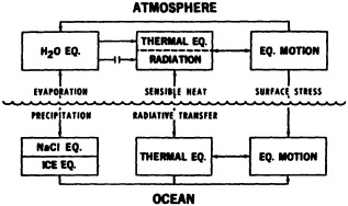
FIGURE 1
Box diagram of coupled-model structure. (From Manabe, 1969b; reprinted with permission of the American Meteorological Society.)
given in Neelin et al. (1992), and a full intercomparison of the climatology of this type of coupled model in Mechoso et al. (1995).) These models tend to have the oceans active only in selected regions; elsewhere, the ocean is relaxed to climatology, while the atmosphere has global extent.
PROBLEMS WITH GLOBAL CGCMS
Coupled models used to simulate ENSO (such as Philander et al., 1992) generally have only the tropical ocean active and use enhanced resolution in the equatorial area. Because these models are designed for interannual studies and are not configured for longer-term variability, they generally lack the mechanisms that maintain the upper ocean's thermal structure, especially the thermohaline circulation (THC), and so gradually diffuse away their thermocline. These models are therefore limited in the length of time over which they can be usefully run.
These types of CGCMs succeed in reproducing some aspects of the time-averaged climate, the annual cycle, and the interannual variability. Unrealistic features persist, however, especially off the western coast of South America, where simulated SSTs tend to be too high. Such problems could be remedied by adjusting the surface fluxes to make the climatology move closer to observed values, but attempts are under way to avoid such "flux corrections" by including or improving parameterizations of the necessary processes—for example, the stratus clouds off the coast of Peru that keep SSTs low.
Global CGCMs used for longer-term studies (e.g., for the response to anthropogenic increases in the greenhouse gases) must correctly simulate the basic climatology of the observed climate system, i.e., they must correctly simulate both the mean state and the annual cycle. It would be most desirable to correctly simulate the climatology without the need for flux corrections. A recent CGCM of Manabe and Stouffer (1988)—a model similar to the one used in the paper of Delworth et al. (1995) in this chapter, but with a sun lacking annual variation—illustrates the difficulties involved in achieving this goal. The model produces a deficit of salt (more properly, an excess of fresh-water) at high latitudes and prevents the deep sinking of ocean parcels. As a result, the THC does not exist, and the heat and salt transports into high latitudes are reduced. The higher latitudes are thus too fresh and too cold, and sea ice extends too far south, conditions that guarantee that the THC cannot get started. If the high-latitude ocean is artificially salted by a constantly imposed saline flux correction and the THC is on, the circulation is helped to stay on by its own delivery of salt to high latitudes. On the other hand, the artificially imposed salt flux is not, by itself, adequate to start the THC; a steady state exists with imposed salt flux but no THC.
The lessons from the Manabe-Stouffer model are that there can be two climate states (one with and one without a THC) in the presence of identical external forcings, and that it is difficult to achieve a good simulation of the surface salinity field unless both the atmospheric and oceanic processes that control salinity are correctly modeled. Salinity at the surface of the ocean is changed by the difference between evaporation and precipitation, by runoff from land, by freezing or melting of sea ice, by advection and subsequent melting of icebergs, by advection, convergence, and divergence of salinity by ocean currents, and by mixing of salinity downward into the ocean. All of these processes, some quite poorly measured and understood, must be modeled correctly to ensure a proper high-latitude salinity budget and hence a correct THC.
The global annual cycle is relatively well documented in the instrumental record. Since there is no guarantee that a CGCM will respond correctly to the imposition of the annually varying external solar forcing, the modeled annual cycle provides a major test of CGCMs. But if a CGCM responds only annually to an annually varying sun, it would miss the variability on all other time scales that comprise the climatology: The annual cycle is the long time average over all the variability present, and variability other than annual may contribute to the observed annual cycle. Since at present flux corrections are still needed to prevent climate drift of CGCMs, the global annual cycle in these models cannot be considered to have been independently modeled.
VARIABILITY
Since the ENSO cycle is so important a signal in the tropical atmospheres and oceans, it is not surprising that inter-decadal modulations of this signal are also important. Rasmusson et al. (1995, in this chapter) present evidence that the ENSO is modulated by long (century-scale) variability, although they make the point that the records are not nearly long enough (or good enough) to characterize this variability more precisely. Cane et al. (1995, also in this chapter) speculate that such regimes of enhanced or suppressed ENSO variability are internally generated, at least in the Zebiak-Cane model, and show that longer data records might be capable of resolving the precise mechanisms. Trenberth and Hurrell (1995, in this chapter) hypothesize that North Pacific decadal variability, which is connected with the Pacific North American pattern, can be linked to this decadal variability of the ENSO phenomenon.
At this time no CGCM that has a resolution near the equator high enough to simulate the processes known to be important for ENSO, has produced (or can produce) long enough simulations to tell us whether such regimes exist. In order to be able to run these models for long periods of time, equatorial high resolution in the ocean must be combined with the accurate simulation of the THC; satisfying both these conditions in the ocean component of a CGCM
is beyond the capabilities of the present generation of supercomputers.
It used to be thought that the response time of the THC was so long that decadal and longer variability would occur simply as a result of the accumulated response of higher-frequency forcings from the atmosphere. Recent results (see Weaver, 1995, in this volume) have indicated that there exist purely oceanic mechanisms for the generation of interdecadal variability, namely, the internal dynamics of the THC itself in response to steady fresh-water forcing from the atmosphere.
The question arises as to whether or not such variability would be present in a fully consistent CGCM, i.e., whether or not the atmosphere would increase or damp the THC variability that would exist in an ocean-only model. The paper by Delworth et al. (1995) in this chapter describes a fully coupled model, driven by an annually varying sun, that has high-latitude salt-flux corrections and heat-flux corrections, both varying as a function of the time of year. The results indicate that inter-decadal or longer variability survives the coupling. The mechanism for the SST and surface salinity involves the variability of the oceanic THC but is modified and complicated by the feedbacks inherent in a fully coupled model.
FUTURE PROBLEMS
Coupled models are gradually coming into their own. They have been quite successful at enabling us to understand and predict a wide range of phenomena, from the ENSO cycle to the responses to the anthropogenic increase of the radiatively active gases, especially carbon dioxide (see, e.g., Manabe et al., 1991, 1992). As computer resources become more available, coupled models are being run at more and more institutions. While it is still true that higher-resolution CGCMs can be run only on supercomputers, the advent of workstation computing has now made it possible for individual investigators to begin to run similar coarse-resolution coupled models.
The success of coupled models depends on the ability of the component models to realistically simulate key climate processes. It is therefore true, and always will be, that progress in atmospheric and oceanic modeling will prompt progress in coupled models. It is also true, however, that coupled models require special attention to processes not ordinarily emphasized in decoupled modeling. For example, atmospheric models must now consider the details of boundary-layer processes near the ocean surface in order to successfully simulate the fluxes of heat and momentum in response to a given SST. Similarly, mixed-layer processes in the ocean must be able to successfully simulate the SST for specified fluxes of heat and momentum from the atmosphere. The distribution of atmospheric rainfall, runoff from land, and sea ice growth and advection become important processes in guaranteeing the success of THC simulation. Because each of the component models is very sensitive to small errors in the other, process simulation that would be acceptable in a decoupled model can lead to unacceptable results in a coupled context. Successful simulation of one component in response to forcing in the other is a necessary, but by no means sufficient, condition for the success of the coupling.
We see that successful coupling demands improvements in the component models; indeed, the future of coupled models will depend on such improvements. Flux corrections can provide a temporary fix for model problems, but totally believable coupled models require simulating accurate climatologies without the need for flux corrections. Simulating decadal and longer variabilities also requires ocean models that correctly maintain the upper ocean's thermal structure; in practice this means that the THC must be correctly modeled. In order to confirm that natural variability has been successfully simulated, longer and more accurate data sets must be available. In this regard, paleoclimate indicators become especially valuable, and other proxy data sets (tree rings, corals, sediment cores, ice cores, etc.) become essential to mapping the domains of variability in which to test the coupled models. In this chapter Battisti (1995) points out not only the unique role that proxy data play in modeling but also the equally unique role that understanding and exploration through modeling play when data are so sparse and difficult to come by.
The ultimate test of understanding and simulating climate variability is the ability to predict that variability. We now know that certain aspects of seasonal-to-interannual variability, especially aspects of ENSO, are predictable, but no one knows whether decadal variability is deterministically predictable—and, if it is, which data are needed as initial conditions. Even if longer-term variability is not predictable, the ability of models to successfully simulate the spectrum of climate variability is a necessary prerequisite to our full understanding of the natural climate system.
CONCLUSION
As we have seen, the basic problem in coupled modeling is the correct simulation of the climatology, particularly the annual cycle. Since climate variability and the annual cycle contribute to each other, this goal is something of a moving target. We have to simulate the annual cycle correctly in order to simulate variability, but we have to simulate the variability correctly in order to simulate the annual cycle. We may therefore expect progress to be rather slow.
Progress in coupled modeling will be accelerated by:
-
Improvements in understanding and modeling the atmosphere, ocean, land, and cryosphere separately. The primary physical processes needing better parameteriza
-
tion are clouds and water vapor in the atmosphere, mixing in the ocean, evapotranspiration and small-scale hydrology in the land, and sea-ice extent and growth in the cryosphere.
-
Advances in understanding the nature of coupling, especially the general question of the sensitivities of each system to small errors in the other.
-
General increases in available resources and computational infrastructure, allowing a wider community to gain access to coupled modeling.
-
Improvement and extension of time series of physical quantities in the atmosphere, ocean, land, and cryosphere. This can be achieved by reanalysis of existing model data (e.g., daily weather analyses), data archaeology, improvements in existing observing networks and data handling, new techniques of paleoclimate analysis ... or by instituting new measuring networks and waiting till the time series is long enough.
While this last technique may seem the least efficient, future generations will appreciate our efforts as much as we would be grateful to previous generations, had they been prescient enough to do the same for us.
Decade-to-Century Time-Scale Variability in the Coupled Atmosphere-Ocean System: Modeling Issues
DAVID S. BATTISTI1
ABSTRACT
A primary limitation in the study of the decade-to-century (hereafter termed "intermediate") time-scale variability in climate is that the instrumental records for all climate variables either do not exist or are too short to detect these phenomena with any measure of statistical confidence. Hence, the methodologies and strategies of the research activities related to the intermediate time scales of climate variability will be distinctly different from those related to interannual variability. While climate models are currently used mainly to simulate phenomena that are already well observed, the models themselves will frequently be the instruments with which scientists identify intermediate-scale climate phenomena. Ascertaining the veracity of a climate model must therefore be a primary activity in the study of intermediate-scale climate variability. Proxy data will play an important role in documenting climate variability on intermediate time scales and in evaluating the climate variability simulated by the models.
In this paper I argue that it is extremely important that the models used for intermediate-scale climate studies be validated a priori by assessing how accurately many well-documented "target" phenomena are represented in each model. Specific target phenomena are suggested, such as the seasonal and diurnal cycles of the state variables that are well-documented in nature, and the fluxes of energy and mass at the media interfaces. A quantitative comparison should be made of the processes that are responsible for these cycles in the model and those that are observed. In addition, valuable information on the veracity of the models will result from an assessment of how well the model's performance matches the well-documented interannual variability in the climate system.
INTRODUCTION
An increasing number of earth scientists have become interested in understanding natural variability in the climate system on century and especially on decadal time scales. This paper pertains to the climate variability within the atmosphere and ocean system on these time scales, which will be referred to as the "intermediate" time scales.2 The potentially critical role of the land hydrology and cryosphere for the intermediate-time-scale fluctuations in climate is discussed elsewhere (see the Atmospheric Observations section of Chapter 2). The variability in the atmosphere-ocean system on the intermediate time scales is poorly documented at present by comparison with both shorter (interannual) and longer (e.g., 103 to 106 years) time-scale oscillations. Information on the longer-scale variability is abundant because the transitions between glacial and interglacial conditions are large enough changes in the global climate system to be clearly defined in the global geological record—e.g., in the stratigraphy of the sediment and ice deposits, and in the radio-isotopic composition and distribution of the embedded flora and fauna. These proxy data have been instrumental in the studies of long-term climate variability because an accurate measure of the absolute elapsed time is available from the decay of the isotopes of the ubiquitous carbon.
Compared with the sub-millennial vacillations in climate, the variability of the climate system on the intermediate time scales is thought to be rather small in amplitude. Until recently, there was little direct evidence for either local or global inhomogeneous climate variations on these time scales. The instrumental records of the climate variables prior to the turn of the century are, in isolation, inadequate for documenting the decade-to-century-scale climate variability; they exist for only a limited number of state variables, and the data for these variables are largely confined to very near the earth's surface (usually within 10 m) and are sparsely distributed. Historians and scientists have used phenological data to infer variability on interannual time scales. Phenological data are, by definition, available only in the regions of human habitation and are susceptible to the vagaries of human perception. In his seminal contribution to the study of European history, Braudel (1949) combined the evidence from literary references with a variety of phenological data and concluded that the entire Mediterranean area experienced abnormally cold and wet winters in the early seventeenth century—the Little Ice Age. (Braudel's data included the time of year of river and lake floods, the years of significant frost damage to olive trees, and the times and yields of various agricultural harvests.)
A much more rigorous historical portrait of the climate variability on intermediate time scales is provided by proxy data, although they are limited in usefulness because their interpretation is not straightforward. Proxy data relevant to intermediate-scale climate variability include d18O concentration in glacial ice, lake varves, loesses, pollen data, and coral and tree-ring data (see, e.g., Bradley, 1991). The proxy and phenological data have been used together to construct a rather detailed and comprehensive assessment of the change in climate since the Little Ice Age; a brief summary is presented in Crowley and North (1991).
In the early 1960s Stommel and Bjerknes published studies that had a benign impact on the community for more than two decades, and now provide focal points for scientists working on the intermediate-scale climate variability. Stommel (1961) hypothesized that the general thermohaline circulation of the oceans might have multiple stable regimes, and demonstrated this hypothesis using a two-box analog model for an ocean basin. Stommel's hypothesis is supported by the recent coupled atmosphere/global-ocean general-circulation model studies of Manabe and Stouffer (1988), who achieved two statistically steady states for the meridional circulation in the Atlantic Ocean—with and without a vigorous thermohaline circulation. Bryan (1986) found that the transition between strong and weak mean meridional circulations in the abyssal ocean could happen in less than a century in a sector ocean model. Recently, Levitus (1989a,b) demonstrated that there was a change in the deep North Atlantic hydrographic structure from the 1950s to the 1970s, and supposed this change to be associated with deep convection (Figure 1). Together, these studies and related analytical, modeling, and observational studies have elevated the deep ocean circulation into the arena of potential mechanisms for—or indicators of—climate variability on the intermediate time scales.
In 1964, Bjerknes examined the contemporaneous fields of sea surface temperature (SST) and sea-level pressure (SLP) from the North Atlantic Ocean and noted differences in the 5-year mean climatologies of 1920-1924 and 1930-1934 (these pentads were chosen on the basis of the Azores-minus-Iceland SLP index). Bjerknes argued that these differences reflected a local climate change resulting from an interaction between the surface gyre circulation of the North Atlantic and the overlying atmosphere. He also implied that there were quantitative changes in the oceanic equator-to-pole heat transport. In retrospect, it can be seen that Bjerknes's method for inferring decadal changes in the pentads' means was inappropriate; the interannual variability of the coupled atmosphere-ocean system in the North Atlantic is large (see, e.g., Wallace et al., 1992; Kushnir, 1994), so a
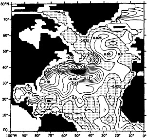
FIGURE 1
The difference in density (in kg m-3) at 500 m depth between the two pentads, 1970-74 and 1955-59. Regions with negative values are stippled and denote higher density during the 1955-59 pentad. (From Levitus, 1989a; reprinted with permission of the American Geophysical Union.)
long-term change inferred from differences in 5-year means is extremely unreliable. Nonetheless, Bjerknes's hypothesis that ocean dynamics play an important role in interdecadal variability is supported by recent studies of the decadal variability of the North Atlantic atmosphere-ocean system (e.g., Kushnir, 1992; Pan and Oort, 1983).
Nearly all the numerical and theoretical research activities on intermediate-scale climate variability have taken place during the last half-decade, for a variety of reasons. First, there is a growing demand that scientists assess and predict the anthropogenic impact on climate. Essential (but insufficient) to accomplish this goal are an accurate statement of the present climate from observations of the state variables, a rigorous program that results in multiple independent forecasts of the anthropogenically forced change in climate, and a comprehensive inventory of the intermediate variability in the present natural climate system so one can plan an efficient monitoring strategy to confidently assess the accuracy of the forecast climate change from the future observed climate.
There is another reason why the interest in the intermediate time scale variability of the climate system has sharply peaked during the past 5 to 10 years that is external to the greenhouse warming problem. The TOGA and EPOCS programs of the 1980s resulted in the documentation, simulation, and skillful model prediction of the El Niño/Southern Oscillation (ENSO) phenomenon. Through these extraordinarily successful programs scientists have explicitly demonstrated for the first time that rich variability in the climate system can result solely from the interaction between the oceans and the atmosphere. More important, this period of research marked the advent of a new era. With a few notable exceptions, for the first time the atmospheric scientists began to focus on the sub-monthly circulation anomalies in the troposphere, and the oceanographers began to abandon the default assumption of a world ocean in a quasi-steady state.3
The research activities of the last decade also created a modest population of scientists that are actively performing basic research on both oceanic and atmospheric circulation, and on the response of a climate system composed of atmosphere coupled with the global oceans. As a result, there are now numerous studies that document coordinated interannual variability in the atmosphere-ocean system, and many studies wherein isolated phenomena have been simulated and the essential physics documented. Thus, the extraordinary interest of the scientific community in identifying and analyzing the variability in the full climate system on decade-to-century time scales through modeling and observational studies can be attributed to both the research focus on the interannual variability of the coupled atmosphere-ocean climate system and the practical problems that have arisen in the detection of an anthropogenically forced climate change.
In this paper, I discuss the constraints inherent in assessing both the actual variability of the climate system on the intermediate time scales and the physical and dynamical processes that are likely to be responsible for this variability. The methods for validating the "modes" of intermediate-scale climate variability that are produced by numerical and analytical models necessarily represent a change from the traditional modus operandi. A good example of the unique blend of modeling and observational research and monitoring efforts that is required to assess intermediate-scale variability is found in the charter for the Atlantic Climate Change Program (ACCP) of the National Oceanic and Atmospheric Administration (NOAA). I describe the ACCP and briefly review the evidence for a directly observed variability in the atmosphere/ocean/sea-ice system that has recently become a focus of the ACCP. The implications for modeling and modeling strategies are discussed, and a summary is presented at the end of the paper.
THE LIMITATIONS OF THE HISTORICAL INSTRUMENTAL RECORD
The primary limitation on the study of climate variations on the intermediate time scale is that the instrumental record
for all climate variables is too short to permit the detection of these phenomena. Prior to the 1950s, the only maritime instrumental records useful for these studies are those for SST and air temperature. Although SST data are available along the major global shipping routes from about 1900 (see, Pan and Oort, 1990), spatial and temporal coverage for these variables is adequate only across the North Atlantic (Figure 2). For the continental areas, potentially useful data are available for more of the climate variables as far back as the mid-1800s. These data, however, are uneven in their spatial distribution. Prior to World War II there are essentially no instrument-based data for the state of the atmosphere above the surface. For the ocean, subsurface data are limited to infrequent and isolated transects through the ocean, usually across the North Atlantic. Thus, prior to the 1950s the instrumental data records exist for only a few key variables in isolated regions, and provide only a blurred glimpse at climate variability. The data are insufficient for deducing the attending atmospheric and oceanic circulations and heat transport, and the energy exchange between the media.
The post-World War II instrumental data base for the
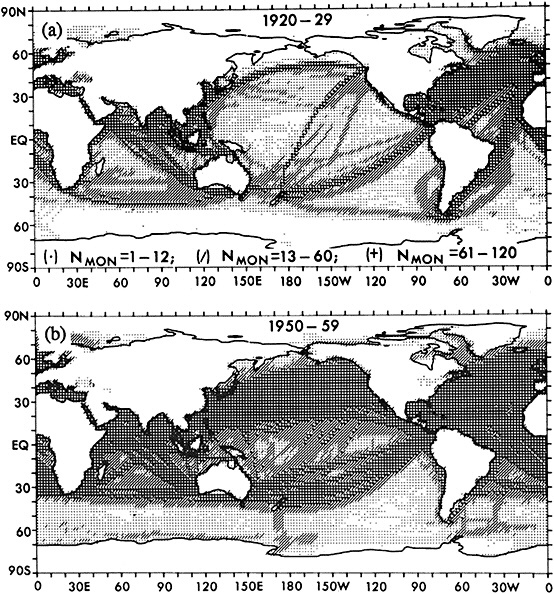
FIGURE 2
The climatological data base for sea-surface temperature. Shown in (a) is the number of months in which there exists at least one observation in a 2° latitude by a 2° longitude area during the decade 1920-29. A dot indicates 1-12 months (out of 120) with data, a slash 13-60 months, and a plus sign 61-120 months. Panel (b): as in (a), but for 1950-59. (From Pan & Oort. 1990; reprinted with permission of Springer-Verlag.)
state of the atmosphere is rather complete4 over the Northern Hemisphere, especially over the continents, but it is not suitable for studying decadal climate variability in the Southern Hemisphere. A very uneven spatial and temporal record of the hydrographic and current structure of the world oceans is available starting after World War II, but it is unlikely that the data coverage is sufficient permit deduction of a posterior decadal variations in the ocean climate.
Fundamental to understanding the coupled atmosphere-ocean system is a knowledge of how energy and constituents are exchanged between the two media. On this score, even the recent instrumental record is clearly deficient. For example, there is large uncertainty as to the annual cycle of the turbulent exchange of heat and momentum alone; estimates of the variability in these energy exchanges on the intermediate time scales would be premature.
In summary, it is not possible to discern the past variability of the climate system on the century scale from the instrumental data sources. Recent decadal variations in the atmosphere-ocean system can perhaps be deduced with some confidence from the instrumental data base, although incompletely. The ample spatial voids in the data set (especially in the subsurface oceans) introduce some uncertainty, into determining whether the variability is locally confined or is of global extent. Because of the severe limitations of the existing instrumental record, proxy data sets will play an important role in documenting the intermediate-scale climate variability and, perhaps, in evaluating simulated climate variability (discussed below).
THE TRADITIONAL MODUS OPERANDI AND THE ATLANTIC CLIMATE CHANGE PROGRAM
The Traditional Modus Operandi
The history of atmospheric sciences and oceanography is replete with examples of community-wide intensive research activities that are focused on the precise documentation and analysis of specific, observed phenomena that represent perturbations from a mean (state) that are statistically significant, e.g., the mid-latitude cyclone, the Quasi-biennial Oscillation (QBO), and the Gulf Stream. Major programs have also commonly had as a centerpiece a well-observed phenomenon. Examples include GATE (easterly waves, mesoscale tropical convection), POLYMODE (long-lived coherent eddies in the ocean thermocline), ERICA (rapidly deepening cyclones), CLIMAP (reconstruction of the climate of the last ice age), and the upcoming EPOCS effort (the annual cycle and the boundary layer circulation in the Pacific).5
The Tropical Ocean and Global Atmosphere (TOGA) program provides a good illustration of the traditional research strategies, and the profound effects the limited data base will have on the modus operandi in research on the variability of climate on intermediate time scales. The ENSO phenomenon was the centerpiece for TOGA, although mid-latitude phenomena were also documented and modeled in this program. It is important to recall that prior to TOGA the ENSO was already a reasonably well-documented phenomenon, being a large-scale, large-amplitude perturbation in the atmosphere-ocean system. The emphasis of the TOGA program was on providing an understanding of how and why this climate anomaly was manifested and assessing the predictability of the phenomena. In contrast, for intermediate-scale climate variability the target phenomena are smaller in amplitude, are derived from only a few realizations, and are not completely defined by the historical data.
The methodologies and strategies of the research activities related to the intermediate-scale climate variability will be distinctly different from those related to interannual variability for two additional reasons: (1) the inherent limitations of the data base of directly observed climate state variables (discussed above), and (2) the constraints imposed by limited computational resources coupled with the uncertainty as to the veracity of the simulated phenomena because of the parameterization of the small-scale processes and the (still) poorly understood physics. The science plan, priorities, and ongoing activities of the ACCP and of the nascent Global Ocean-Atmosphere-Land System program (GOALS) duly reflect these constraints.
The Atlantic Climate Change Program
The ACCP was formally initiated after a workshop held at the Lamont-Doherty Earth Observatory of Columbia University in July 1989. The goals of this program are as follows:
-
To determine the seasonal-to-decadal and multidecadal variability in the climate system due to interactions between the Atlantic Ocean, sea ice, and the global atmosphere using observed data, proxy data, and numerical models.
-
To develop and utilize coupled ocean-atmosphere models to examine seasonal-to-decadal climate variability in and around the Atlantic Basin, and to determine the predictability of the Atlantic climate system on seasonal-to-decadal time scales.
-
To observe, describe, and model the space-time variability of the large-scale circulation of the Atlantic Ocean and determine its relation to the variability of sea ice and sea surface temperature and salinity in the Atlantic Ocean on seasonal, decadal, and multidecadal time scales.
-
To provide the necessary scientific background to design an observing system of the large-scale Atlantic Ocean circulation pattern, and develop a suitable Atlantic
-
Ocean model in which the appropriate data can be assimilated to help define the mechanisms responsible for the fluctuations in Atlantic Ocean circulation.6
The ACCP is an interdisciplinary program that involves atmospheric scientists, oceanographers, and paleoclimatologists. Currently the program shows an appropriate balance between modeling efforts and analysis of the historical proxy and instrumental data. Furthermore, observational programs have been launched to help determine the link between intermediate-time-scale SST anomalies and variability in the thermohaline circulation by means of long-term monitoring of the deep Western Boundary Current. Observational studies that are ongoing or anticipated include tracer inventories, hydrologic monitoring of Fram Strait, and monitoring of the upper ocean thermal structure through the Atlantic Voluntary Observing Ships Special Observing Project and surface-drifter deployments.
Two different patterns of variability in the North Atlantic atmosphere-ocean system have been identified in the historical data. Deser and Blackmon (1991; 1995, in this volume), using the historical observational data of sea-surface temperature, sea-level pressure, and the zonal wind over the Atlantic Basin, have demonstrated that there is a complex wintertime atmosphere-ocean interaction in the North Atlantic with a preferred time scale of about 10 years. The anatomy of this decadal variability appears to be somewhat different from that of the interannual climate anomaly in the North Atlantic documented in Wallace et al. (1992).
Using the same surface fields and focusing on the changes in the Atlantic atmosphere-ocean system over multidecadal periods during the last century, Kushnir (1992) found the relationship between changes in the SST and changes in the overlying surface atmospheric circulation significantly different from that associated with higher-frequency variability in the Atlantic climate system. In this multidecadal transition, the atmospheric circulation changes are consistent with a local quasigeostrophic response to the changes in the ocean SST (see Figure 3). The hydrographic record for the same period indicates that the SST changes are echoed in the deep ocean, where concomitant changes in salinity are found (Lazier, 1988; Levitus, 1989a,b; see also Figure 1). Thus, as is not true for the higher-frequency "modes," evidence suggests that changes in the thermohaline circulation and sea-ice export from the Arctic Ocean are associated with this multidecadal transition.
In order to identify the climate variability in and around the Atlantic basin on decade-to-century and longer time scales, ACCP-sponsored studies have been begun that will determine the extent to which the instrumental records used in the studies mentioned earlier can be augmented (e.g.,
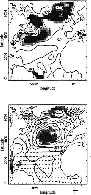
FIGURE 3
Decadal time-scale climate anomalies in the wintertime (December-April) in the North Atlantic Panel (a): the difference between the average wintertime SSTs between 1950 and 1964 and between 1970 and 1984. The former period (1950-1964) was characterized by warmer-than-normal water in the winter in the North Atlantic, the latter (1970-1984) by anomalously cold water. The contour interval is 0.2°C. Panel (b): as in (a), except for the attendant atmospheric surface variables: sea-level pressure (contour interval 0.5 mb) and vector winds (a 1.0-m/s vector is found below the panel). (From Kushnir, 1994; reprinted with permission of the American Meteorological Society.)
surface salinity and hydrographic data). Nonetheless, the state of the (Atlantic) climate system, as realized from direct measurements of the climate state variables, will remain insufficient to permit assessment of the natural climate variability on decadal and longer time scales, especially away from the earth's surface. Thus, within the ACCP there are also ongoing studies to identify sources of proxy data that will define and constrain the variability in the Atlantic climate system. These studies include an analysis of dendroclimatic and ice-core data surrounding the North Atlantic as well as an analysis of deep-sea, high-sedimentation-rate cores. Encouraging preliminary results from these studies were presented by D'Arrigo et al. (1992), Bond et al. (1992), and Keigwin and Boyle (1992) at the 1992 ACCP Principal Investigators' meeting.
The usefulness of a single proxy data source for inferring the intermediate-time-scale variability in climate or a climate state variable is often limited for two reasons. First, common proxy data are not usually available for the entire globe (e.g., coral is found only in the tropics). Thus, a proxy source, in isolation, cannot be used to differentiate local and global climate variations. Second, climatic implications from a single proxy source can be ambiguous. For example, the cambial activity of trees depends on both seasonal temperatures and precipitation; for many species of trees it is difficult to determine uniquely the relationship between these two climatic variables and the cambial activity. Many proxy climate indicators must be used to ensure consistency and remove any ambiguity in the historical climate record assembled from the proxy data, and to better assess whether the climate variability is regionally confined or global in extent. The utility of this effort is illustrated by the remarkable progress made on the climate of the last glacial maximum (CLIMAP, 1981). In this regard, the IGBP Past Global Change project (PAGES) is timely (IGBP, 1992; see also Bradley, 1991).
IDENTIFYING POTENTIAL CLIMATE VARIABILITY ON DECADE-TO-CENTURY TIME SCALES FROM NUMERICAL MODELS: STRATEGIES AND LIMITATIONS
Numerical models will be the primary tools by which the mechanisms responsible for decade-to-century-scale climate variability are identified. More important, these same models will frequently be the instruments that scientists use to identify target intermediate-time-scale climate phenomena, because instrumental data exist only for the last century and, as mentioned above, for only a limited domain of the climate system. For the same reasons it will often be difficult to determine whether simulated phenomena are ever realized in nature. Thus, our confidence that a simulated phenomenon could occur will result only from an a priori assessment of how accurately the model simulates many well-documented phenomena.
A model to be used for studying natural variability in the climate system on the intermediate time scales must include complete and interactive modules for the four central media: the atmosphere, global oceans, the global terrestrial marine biosphere, and sea ice. An important aspect of this system for the intermediate-time-scale climate studies is an accurate and complete representation of the hydrologic cycle (OCP, 1989). Climate variability models are the result of marrying the individual models for the four media, each of which has first been tested in isolation by prescribing the appropriate boundary conditions for the state of the adjacent media. (When appropriate, the flux of energy is prescribed at the boundaries.) The tests of the uncoupled models do not guarantee a good coupled climate model, but are practical first steps.
Finally, full general-circulation models (GCMs) for the atmosphere and global oceans are required to study the intermediate-time-scale climate variability. There is no evidence from the observational data that the intermediate-time-scale climate variability is regionally confined—for example, to within a hemisphere, an ocean basin, or to the near-surface ocean—as the interannual climate variations seem to be.
Prerequisite Constraints for the Uncoupled Modules
The foremost test of the uncoupled component modules is the ability of the model to reproduce the seasonal cycle, and thus the annual mean state, when forced by the imposed boundary conditions. The annual cycle is an test case for validating uncoupled component modules, because in most cases the annual cycle is well known for many of the climate state variables; in some cases the product moments are also reasonably well known (e.g., the meridional heat transport in the atmosphere). For the coupled atmosphere and land-surface modules, the diurnal cycle provides a second excellent test. The diurnal cycle of near-surface fields of air temperature, moisture, clouds, and wind are well-observed quantities over land. An accurate simulation of these cycles throughout the year provides a rigorous test of the impact of the combined boundary-layer physics and surface-flux parameterizations that act to maintain the simulated climate.
The general-circulation models for the atmosphere (AGCMs) are routinely validated by comparing the simulated climatology with that observed for variables or features that include the jet structure, variation of the height of selected geopotential surfaces in the troposphere, the zonal mean distribution of temperature, zonal wind, and SLP. It is of crucial importance for climate variability, however, that the models accurately simulate the observed annual cycle of all the boundary-layer fluxes: momentum, sensible, convective, latent, and radiative fluxes at the surface, and outgoing long-wave flux at the top of the atmosphere.
The sea-ice models should be required to provide an adequate simulation of the seasonal cycle of surface temperature, sea-ice thickness, and ice advection and production—all quantities that are qualitatively known from observations (e.g., Walsh et al., 1985). The ocean models must be able to simulate the climatological annual mean circulation and hydrographic structure. In the tropics there is a significant and well-documented annual cycle in the upper-level currents and hydrography that provides additional constraints on the model. Especially important is the accurate simulation of the global SST. Until recently the SST was constrained in many ocean modeling studies by a rapid forced relaxation to a prescribed climatology.
A relaxation to a climatologically observed hydrography has also been used in and below the thermocline in many numerical studies of ocean general circulation (Hibler and Bryan, 1987; Semtner and Chervin, 1988); in some instances maintenance of the thermocline is avoided by limiting the length of integrations, so equilibrium is never achieved. This practice has been useful for short-term simulations of the upper-ocean circulation away from convective regions (e.g., Philander et al., 1987) but is clearly inappropriate for the study of climate and intermediate-scale climate fluctuations. The limited observational data indicate that the entire ocean domain can be involved in climate variations on these time scales (e.g., Levitus, 1989a), although it is not clear, for instance, whether the deep ocean is necessarily an active player or just a barometer for the changing surface processes via the resultant convection.
Independent tests of the component models should also include constraints that can de deduced from certain tracers that are well observed and whose annual cycle and mean distributions are understood. For the atmosphere, these include the 85Kr, Freons, and CO2, which have already been used to independently validate the mean cross-equatorial exchange rate of one AGCM (Tans et al., 1989). For the ocean, the bomb-produced tracer 14C can be utilized to assess the accuracy of the simulated Atlantic Ocean circulation and the concomitant mixing processes (Toggweiler et al., 1989). Further insights into the oceanic mixing processes and convection, both of which are parameterized in ocean models, may be obtained by comparing the Lagrangian transport in models with observed distributions of other tracers, including the chlorofluorocarbons.
Finally, there are well-observed phenomena in the atmosphere and ocean that occur on interannual time scales that can be used to help validate the models. For the atmosphere models these include the QBO and the Southern Oscillation, and for the Pacific Ocean models, the El Niño.
There is a tremendous amount of work to be done on documenting the impact of the parameterization of unresolved physics on the simulated large-scale, low-frequency climate. Recent studies have demonstrated that different parameterizations for convection in both atmosphere and ocean GCMs can result in qualitatively different mean circulations and climate variability; an example is discussed below. Similarly, the recent advances in understanding the dynamics and thermodynamics of individual clouds must be extended to yield quantitative descriptions and parameterizations of the energy and mass transport by an ensemble of clouds on the scale of an AGCM grid.
Recent Results: Overturning the Rocks
In this section I will use three examples that I believe presage the results that will be achieved during the 1990s in modeling intermediate-time-scale climate variations.
Example 1. Over the last decade, studies have been published on the response of the wintertime Northern Hemisphere atmosphere to the principal mode of the observed interannual SST anomaly in the North Pacific Ocean (e.g., Pitcher et al., 1988). In these studies, which utilized AGCMs, investigators prescribed a perpetual January insolation to ensure statistically significant results with limited computational resources. The model's response to the prescribed SST anomaly in each of these experiments was contrary to that observed (e.g., Wallace and Jiang, 1987). The polarity of the model's geopotential anomaly was independent of the polarity of the forcing anomaly. Recently, Lau and Nath (1990; hereafter LN) examined the response of the GFDL AGCM to the observed 1950-1979 SST and an annual cycle in insolation.7 Upon isolating the circulation anomalies associated with the North Pacific SST anomalies, LN found that the model anomalies were indeed consistent with those observed (i.e., a quasi-linear relationship between anomalies in SST and geopotential). Kushnir and Lau (1992) used the same model as LN and repeated the perpetual-January experiments of Pitcher et al. (1988). The results of this study were consistent with those of the earlier perpetual-January experiments, and contrary to LN and the observational data. Thus, the discrepancies between the physics of the observed atmospheric response to SST anomalies and that found in the simulations of Pitcher et al. and of Kushnir and Lau can be explained by the prescribed unrealistic (perpetual-January) forcing. The moral here is that compromises in the experimental plan that are made because of computational constraints may lead to fallacious conclusions.
Example 2. James and James (1989) employed a primitive-equation model of the atmosphere (T21, five layers), prescribing the annual cycle as the only long-term forcing; slow variations in SST or insolation were not permitted in their experiment. In this model, the variance in the largest-scale structures in the circulation was on a decadal or longer
time scale (Figure 4). Here the moral seems to be that variability on the intermediate time scale may be internal to one or more of the principal climate media, and coincidental to any variations in either the external forcing or in the surrounding media.
Example 3. A similar cautionary note is found in the studies of Weaver and Sarachik (1991a,b; hereafter WS). WS employed a stand-alone ocean-sector model to examine the variability in the thermohaline circulation (THC). They found that under steady mixed surface-boundary conditions (i.e., linear relaxation to a prescribed surface temperature, and a flux boundary condition on surface salinity) the meridional circulation was not steady; rather, three ''climate states" were realized: a collapsed THC, a vigorous THC, and a stage with highly energetic decadal oscillations in the circulation. The decadal oscillations result from the interaction between the convection in the polar regions and the buoyancy advection in the subtropical and polar-gyre circulations (Figure 5). These oscillations are accompanied by up to a threefold change in the poleward transport of heat. Throughout the oscillation, the deep ocean essentially acts as a reservoir, and thus works to maintain the long-term mean thermocline. Eventually, the THC collapses, and the decadal oscillations cease. The WS studies clearly indicate the potential for rich and unexpected intermediate-scale variability that is internal to the ocean.
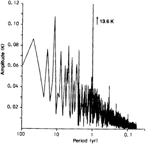
FIGURE 4
Spectrum of mean pole/pole temperature difference from a 96-year integration of an atmospheric primitive-equation model. The only long-term forcing is a prescribed annual cycle in the radiative relaxation temperature; no energy exchange is allowed at the surface of the top of the atmosphere. Note the spectral peak at 12 years. (From James and James, 1989: reprinted with permission of Macmillan Magazines Ltd.)
These and additional results presented in WS also serve to illustrate the state of affairs in ocean climate modeling. Here, I will only point out that the stability of the climate states found in WS depended on the type of convective scheme used, the type of boundary condition set for fresh-water, whether synchronous or asynchronous time stepping was used, and the horizontal resolution.
Together, these three examples illustrate the importance of extensive and meticulous examination of all the uncoupled models that will be used to study the intermediate-time-scale variations in climate. Such an examination should document the following prior to constructing a full climate model for use in studying intermediate-scale climate variability: the ability of all models to simulate multiple observed phenomena, the sensitivity of the solutions to the parameterized physics, and the sensitivity of the component models to the chosen numerical methods of solution and to the shortcuts that are motivated by computational constraints (e.g., perpetual-January insolation, asynchronous time stepping).
Validating the Performance of the Coupled Models
The numerical models that will be used to study intermediate-time-scale variability in climate will necessarily allow interactions between the atmosphere and global oceans and include modules for the land-surface hydrology and cryosphere. The climate system models will be validated by comparing the simulated modes of variability with those that are indicated by a careful analysis and synthesis of the multiple, contemporaneous proxy indicators for the global climate state. Stream One of PAGES is a very ambitious program to reconstruct the global climate since 2000 years BP using the available proxy data sources collectively. The temporal resolution of this climate record is expected to be decadal or better, so the reconstruction will provide the modeling community with "target" phenomena. The data from this program, which is not yet under way, will not be available for quite some time. It is reasonable to assume, however, that the climate models least prone to yielding non-physical solutions on the intermediate time scales are the models that can accurately simulate many of the directly observed and well-documented higher-frequency phenomena in the climate system. Thus, a prerequisite for a model for intermediate-time-scale climate studies is accurate reproduction of many of the already well-observed target phenomena and features.
The same target phenomena that are appropriate for testing the stand-alone component models are also appropriate for testing the climate system model. For example, the system model should adequately simulate the observed diurnal cycle in the near-surface atmosphere over land. It also should accurately simulate the annual cycle in each medium, especially for the state variables adjacent to the media inter-
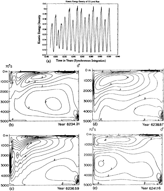
FIGURE 5
(a) The temporal variation in the kinetic energy density in an ocean-sector model, forced by "mixed" boundary conditions. The regular oscillations at 8.6 years are associated with cyclic changes in the meridional overturning circulation; the four characteristic stages are displayed in panels (b) through (e). Positive contours denote clockwise transport. (From Weaver and Sarachik, 1991b; reprinted with permission of the Canadian Meteorological and Oceanographic Society.)
faces and for the energy and mass exchange between the media. Wherever possible, both annual and diurnal cycles should be validated against those observed.
Important new constraints are available to the climate system model on the annual and especially the interannual time scales. Subtle discrepancies between the observed and simulated interfacial fields and fluxes formed with the standalone atmosphere and ocean models are often amplified in the coupling process. This amplification leads to a coupled climate state that is qualitatively different from either of the states achieved by the two uncoupled models in isolation. These "setbacks," however, are fruitful because they often indicate a physical deficiency in a component model that, when corrected, yields a more accurate climate model. The unpublished studies by Gordon (1989). Latif et al. (1988), and Mechoso et al. (1991) provide excellent examples of
how the coupling of atmosphere and ocean models can be used to identify the subtle but key processes involved in the maintenance of the present mean climate.
The observations also clearly demonstrate that certain coordinated atmosphere-ocean modes on the interannual time scale exist only because of the interaction between these media. The most robust example is ENSO, although there is increasing evidence for one or more western Northern Hemisphere coupled atmosphere-ocean modes. The absence of these unforced natural "modes" or phenomena in a climate system model can be helpful in isolating serious deficiencies in the model physics or in the formulae that govern the exchange of energy and mass between the media.
CONCLUSIONS AND DISCUSSION
Within the scientific community interest is growing in identifying and analyzing the variability in the full climate system on decade-to-century, or intermediate, time scales through modeling and observational studies. The resulting increased research activity can be attributed both to the advances in research on the interannual variability of the coupled atmosphere-ocean climate system and to the practical problems that have arisen in the detection of an anthropogenically forced climate change. The primary limitation on the study of climate variation on the intermediate time scale is that the instrumental records for many climate variables either do not exist or are too short to detect a phenomenon with any statistical measure of confidence. Proxy data for climate, therefore, will play an important role in documenting the past climate variability on the intermediate time scales and, most likely, in evaluating the simulated climate variability. This approach represents a significant change from the traditional modus operandi, wherein the models are used mainly to simulate phenomena that are already well observed. The goals and research activities supported by the ACCP illustrates these points.
Numerical models will be the primary tools by which the mechanisms responsible for decade-to-century-scale climate variability are identified and, most important, will frequently be the instruments scientists use to identify the intermediate climate phenomena. Thus, it is extremely important that the veracity of climate system models be evaluated a priori by assessing how accurately they simulate many well-documented phenomena. These "target" phenomena include the seasonal and diurnal cycles of the state variables that are well documented in nature, the fluxes of energy and mass at the media interfaces. Also necessary is a quantitative comparison of the processes that are responsible for these cycles in the model with those that are observed. Other prerequisites for a climate system model should include its ability to simulate the robust natural interannual variability that is observed within the individual media (e.g., the QBO) and in the coupled atmosphere-ocean system.
Where are we now? At present, no climate system models include a satisfactory treatment of the cryosphere and land hydrology for the intermediate-scale climate problem. In fact, there are only two climate models that have the potential to resolve the quantitative three-dimensional circulation of both the atmosphere and the global oceans: the Hamburg model (Cubash et al., 1991, unpublished manuscript) and the GFDL model (Manabe et al., 1992). Both of these models require flux corrections to achieve a mean climatology that is qualitatively consistent with that observed.8 To date these and other models have been used primarily to simulate the climate of the recent ice age and to estimate the potential for large climate changes due to an increase in the atmospheric CO2 concentration (IPCC, 1990; Delworth et al., 1995, in this chapter). These climate perturbations are extremely large in both amplitude and in spatial scale by comparison with the climate variations that are anticipated—and have thus far been observed—on the intermediate time scale. In addition, the agents responsible for the glacial cycles are unlikely to be relevant to the intermediate climate problem. Thus, the success of the climate system models in reproducing geologic time-scale variations will be of little use in assessing the veracity of the intermediate-scale variability that is produced by the same model. For these and many other reasons it is unclear whether the decade-to-century-scale variability produced by any of the existing climate system models has any bearing on the variability in the true climate system.
The research activities over the last 10 years have led to incredible progress in the modeling of climate, especially on the geologic time scales. On the intermediate time scale, significant progress has also been made. Important recent results achieved using stand-alone models of the individual media and the GFDL complete climate-system model will provide a great deal of guidance in establishing the scientific priorities for the next decade. These priorities include improvements in the parameterization schemes for certain small-scale processes, and the identification of key physics through extensive model-sensitivity experiments. The results of studies that address these and other central issues will be instrumental in the design of reliable models of decade-to-century-scale variability in the climate system.
ACKNOWLEDGMENTS
This work was supported by the National Science Foundation (Grant ATM 8822980) and the National Oceanic and Atmospheric Administration's Office of Global Programs and EPOCS. This is contribution number 217 to the Joint Institute for the Study of the Atmosphere and Oceans (JISAO).
Commentary on the Paper of Battisti
GERALD R. NORTH
Texas A&M University
Dr. Battisti's presentation made a broad sweep over many of the issues that we have talked about this week. He has thus given me the opportunity to touch on a few of these in relation to my own paper.
I tend to approach the question of long-time-scale change in an engineering fashion: I wonder whether we can tell from all the different records that we have whether there really is any anthropogenic forcing, and whether we are seeing any response to it. I recognize that there are many other reasons for studying these time scales, but this is certainly an important one. I find it particularly interesting that as we try to make some kind of statistical test of what we have seen in the last century, it is the frequencies just bordering on the decadal range from below for which we really need answers.
I should like to talk a little about two Hasselmann-type models, which could also be called default models. The first one is noise forcing on a mixed-layer slab model with geography; the other one is a deep-ocean extension of that, but still very crude: It distorts the spectrum somewhat at low frequencies. One of the things I noticed as we went through the week—Ed Sarachik and Bob Dickson have already mentioned it—is the failure of these models to generate intermediate water very well. That has a very important impact right in the frequency band (100 yr)-1 to (10 yr)-1. Also, one of the odd things about our deep-ocean model is that it cannot get information down to the thermocline area very well. The giant models adjust so quickly onto the ramp curve that I suspect they might be getting information down there too fast.
All this makes me wonder whether the kinds of things that Jim McWilliams brought up earlier might be fairly serious—for instance, when we construct our bottom topography out of stair steps. Going out in Reynolds number on that lovely bifurcation diagram that he showed is equivalent to going to higher and higher resolution. In our present models we have gone past only a couple of bifurcations, and it is hard to tell whether we are seeing fictitious oscillations in our model world that might go away if we were to go just a little bit further. I do not mean to criticize the people who are working on these models; I think they are doing what needs to be done. Consider, for instance, some of the things that Dr. Rooth and Dr. Barnett showed. I cannot help suspecting that if we were to look at the Mikolajewicz/ Maier-Reimer model, we might see a peak at 300 years (recall the film loop that we viewed earlier this week), and in the Delworth et al. work we might see a peak in the 50-year range. These would, of course, have a large impact on our ability to pick out a signal or to infer how rare such an excursion might be in, say, the last century. Clearly, we have a lot to do before we can unravel these problems, so I again raise Dr. McWilliams's issue.
I should also like to mention once more something that Dick Lindzen pointed out on the first day, since I think it is important but easy to miss. Up at the top of the ocean there is a "valve" that allows the radiation to go out and be absorbed. It amounts to an effective cooling coefficient, with all the feedbacks and everything that must go into it, and thus controls the spectrum and basically the sensitivity of the atmospheric model. If we have an otherwise good atmospheric model that does not do the clouds right, its sensitivity may be wrong by a factor of 2 or even 3, and that error will actually control the spectrum in the low-frequency range. It will have a rather important influence on fluctuations, even at the decadal level.
I hope that Dr. Battisti will open the discussion with some ideas about where we should be going in modeling, and particularly how fine the scales must be to get at some of the questions that we need to answer.
Discussion
BATTISTI: Explicitly examining the mechanisms and processes that yield variations in climate would take more computational power than I for one can fathom, even if we looked at only a subset of the system. I think what we should try for is determining the sensitivity of the simulated climate variability to the parameterization schemes for the unresolved physics. That sensitivity is likely to be a strong function of model resolution.
SARACHIK: You know, it seems to me that we should start concentrating on the signal rather than the noise. Some of the variability we've been talking about is undoubtedly scientifically interesting, but it's relatively local. It seems to be bounded by something on the order of one-third or one-half of a degree of temperature. My inclination is to look at longer time scales, something like 1000 years, and a signal big enough to be called climate change.
REIFSNYDER: I'd like to take philosophical issue with your statement that models are used to test hypotheses. I'd say that models are simply functional expressions of hypotheses, and any meaningful testing must involve independent data sets. Testing against data used in the specification of the model, or against general phenomena, won't tell you anything about predictive power.
BATTISTI: Well, that's true. The solution to a model is really the solution to a set of equations. But what worries me is the possibility that the results of complex, numerical GCMs will be used to build hypotheses of how model phenomena come about, without adequate attention to whether those phenomena appear in the observational or proxy data bases. I'd rather see models used to test hypotheses about the mechanisms responsible for observed phenomena. That is, we should be testing our understanding of a phenomenon, not defining one.
LINDZEN: I think that our interest has traditionally been signal detection—greenhouse warming, for instance. That implicit search for something dramatic worries me. I think we should be equally concerned with the constraints on detectable phenomena provided by the data themselves.
LEVITUS: It seems to me essential that we understand decadal-scale variability better before we can go on to longer time scales or develop better models. First we have to be able to parameterize the processes better and to understand the system on shorter time scales.
WEAVER: The people who complain that this or that process hasn't been included in a model seem not to understand that you can't possibly do a systematic analysis by putting everything in at once.
RIND: A propose of some comments by both Dave and Ed, I'd like to mention again that the NSF/NOAA ARRCC—Analysis of Rapid and Recent Climate Change—program is currently working on reconstructing the big climate changes over the past 1000 years, which includes two cold periods and one warm. We want to put together a worldwide picture of how the climate then compares with today's, and ultimately see whether models can reproduce it.
MARTINSON: Jerry, I just wanted to add that I'm glad you emphasized that it's almost impossible to evaluate the role of sea ice in long-term changes when a model has prescribed flux corrections, since in reality so much of that flux is driven by sea ice itself.
North Atlantic Interdecadal Variability in a Coupled Model1
THOMAS L. DELWORTH, SYUKURO MANABE, AND RONALD J. STOUFFER2
ABSTRACT
A fully coupled ocean-atmosphere model is shown to have irregular oscillations of the thermohaline circulation in the North Atlantic Ocean with a time scale of approximately 40 to 50 years. The fluctuations appear to be driven by density anomalies in the sinking region of the thermohaline circulation combined with much smaller density anomalies of opposite sign in the broad, rising region. Anomalies of sea surface temperature associated with this oscillation induce surface air temperature anomalies over the northern North Atlantic, the Arctic, and northwestern Europe. The spatial pattern of sea surface temperature anomalies bears an encouraging resemblance to a pattern of observed interdecadal variability in the North Atlantic.
INTRODUCTION
Substantial variability in the North Atlantic Ocean occurs on time scales of decades; this variability is thought to be associated with fluctuations in the large-scale meridional overturning (Gordon et al., 1992). This meridional overturning consists of cold, saline water sinking at high latitudes of the North Atlantic and flowing equatorward at depth, upwelling throughout the world oceans, and returning as a northward flow of warm, salty water in the upper layers of the Atlantic ocean. This overturning largely determines the oceanic component of the northward transport of heat from the tropics to higher latitudes and is thus essential for the maintenance of climate in the North Atlantic region (Manabe and Stouffer, 1988). Fluctuations in the intensity of this overturning have the potential to affect climate (Bjerknes, 1964) in both the ocean and the atmosphere. Interdecadal fluctuations in this overturning are thus of potentially critical importance, not only for their direct impact on the climate of the North Atlantic and European regions but also because of the implications of such variability for the detection or modification of anthropogenic climate change. The presence of interdecadal variability in the coupled ocean-atmosphere system makes the detection of anthropogenic climate change more difficult.
The incompleteness of the observational record makes it difficult to study variations in this overturning and the associated processes solely on the basis of the observational data. As a complementary approach, the output from a 200-
year integration of a coupled ocean-atmosphere model is used to study the stability and variability of this meridional overturning (hereafter referred to as the thermohaline circulation, or THC). The output from this model, developed at NOAA's Geophysical Fluid Dynamics Laboratory, forms the basis for the analyses presented here. Several previous modeling studies (Mikolajewicz and Maier-Reimer, 1990; Weaver and Sarachik, 1991b; Weaver et al., 1991; Winton and Sarachik, 1993) have used ocean-only models to study the variability and stability of the thermohaline circulation, in contrast to the fully coupled ocean-atmosphere model employed in the present investigation. Since the mechanisms governing the fluxes of heat and fresh-water across the ocean surface differ substantially between the two types of models, the models might be expected to have different time scales for variations in the THC. While the quantitative results presented here will depend on the details of the model formulation and the physical parameterizations employed, it is hoped that the physical processes identified in this model study are robust and are responsible for interdecadal variability in the North Atlantic. The present study demonstrates that substantial variability can occur in the coupled ocean-atmosphere system on time scales of decades in the absence of external forcings such as changing concentrations of greenhouse gases.
MODEL AND EXPERIMENTAL DESIGN
The oceanic component of the coupled model solves the primitive equations of motion with an approximate horizontal resolution of 3.75° longitude by 4.5° latitude, and 12 unevenly spaced vertical levels. A simple thermodynamic balance is used to predict the presence and thickness of sea-ice, which is advected by surface currents as long as the sea ice thickness is less than 4 m. The atmospheric model solves the primitive equations using the spectral transform technique, and has an approximate horizontal resolution of 7.5° longitude by 4.5° latitude. The atmospheric model, which has 9 unevenly spaced levels in the vertical, incorporates seasonally varying insolation and terrestrial radiation. Cloud cover is predicted whenever the relative humidity exceeds a critical value (99%). At continental surfaces, the heat and water budgets and their interaction with the atmosphere are computed.
The coupled model is global in domain, incorporating realistic geography smoothed to the model resolution. The atmosphere and ocean interact through the surface fluxes of heat, fresh-water, and momentum. The surface fluxes of heat and fresh-water into the ocean are adjusted at each grid point in order to obtain a more realistic simulation of climate. The surface flux adjustments are derived from preliminary integrations of the separate oceanic and atmospheric models. The derived flux adjustments do not vary from year to year and are not dependent on the anomalies of surface temperature and salinity. Thus, they do not explicitly affect the strength of the feedback processes that reduce the anomalies of temperature and salinity at the ocean surface. The model and the flux adjustments are described in more detail in Manabe et al. (1991).
Starting from an initial condition in quasi-equilibrium, the coupled model is time-integrated over a period of 200 years. The mean rate of change of global mean sea surface temperature for the model over this period is very small (0.01°C per century).
RESULTS
Comparison with Observed Variability
An assessment of the model's ability to simulate climate variability is indicated in Figure 1 by comparing a spectrum of model generated sea surface temperature (SST) to a spectrum of observed SST (Frankignoul and Hasselmann, 1977). The observed SSTs are from ocean weather ship India in the North Atlantic (59°N, 19°W), while the model SSTs are from the model grid point closest to the location of ocean weather ship India. Although the model tends to underestimate the total variance (proportional to the area beneath the spectrum), the overall agreement between the two spectra is good.3 One should note, however, that the present model does not resolve mesoscale eddies, which may contribute significantly to the variability of sea surface temperature at seasonal to annual time scales.
Meridional Overturning Index and Variability
The stream function describing the meridional circulation in the Atlantic basin (200-year mean) is shown in Figure 2. The circulation follows the direction of the arrows; its magnitude is proportional to the gradient of the contours. Water flows northward in the upper layers, sinks at high latitudes, and flows southward at depth. The region in which most of the sinking occurs in the model North Atlantic is principally confined to the latitudinal belt from 52°N to 72°N; hereafter, the term "sinking region" will refer to the
|
3 |
In subsequent figures and the text, it is demonstrated that the intensity of the meridional overturning in the model North Atlantic has enhanced variance at a time scale of 40 to 50 years, but the spectrum of model SST in Figure 1 is not characterized by enhanced variance in this frequency band. As shown in Figure 4a, there is a spatial pattern of SST anomalies associated with these overturning variations. The point chosen for the SST spectrum in Figure 1 is not located in this region, and thus does not have enhanced variance at the 40-to-50-year time scale. Spectra of model SSTs from the region of maximum SST change shown in Figure 4a are characterized by enhanced variance at the 40-to-50-year time scale. |
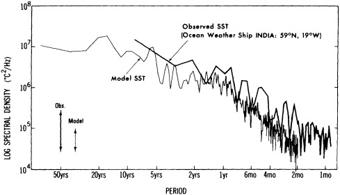
FIGURE 1
Heavy, solid line: spectrum of sea surface temperature from observed data (ocean weather ship India. 59°N, 19°W). Light, solid line: spectrum of model sea surface temperature from grid point closest to 59°N, 19°W. The arrows in the lower left corner denote 95 percent confidence intervals about the spectra. (From Delworth et al., 1993: reprinted with permission of the American Meteorological Society.)
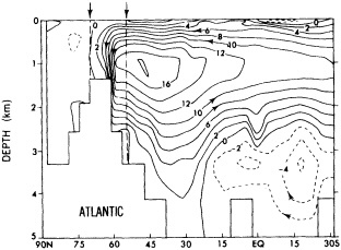
FIGURE 2
Stream function of the meridional overturning in the Atlantic Basin. Flow follows the direction of the arrows. Units are sverdrups (106 m3/s). The dashed lines denote the sinking region as defined in the text. (From Delworth et al., 1993: reprinted with permission of the American Meteorological Society.)
region defined by this latitudinal belt and extending from the western to the eastern boundaries of the Atlantic basin.
In order to concisely describe variations in this meridional overturning, one needs a measure of the intensity of the thermohaline circulation in the North Atlantic. This intensity is defined each year as the maximum stream function value representing the annual mean meridional circulation. A time series of this index, which represents the fluctuations in the intensity of the annual mean THC, is shown in Figure 3a. Visual inspection of this figure reveals substantial variability on interdecadal time scales. The spectrum of this time series, shown in Figure 3b, demonstrates enhanced variance in the 40-to-50-year time scale. Analyses of an extension of this integration (to 1000 years in length) suggest that these irregular oscillations are present in the period beyond 200 years, but are characterized by a somewhat longer time scale. In addition, the spectrum from the longer THC time series contains a more clearly defined broad spectral peak.
It should be noted that the index, by definition, primarily describes variations in the North Atlantic section of the THC. Subsequent analyses show that the climatic variations in the model associated with variations in this index are not hemispheric in nature, but are better characterized as regional to the North Atlantic and Arctic.
Sea Surface Temperature. Salinity, and Surface Air Temperature Variations
The spatial pattern of the changes of model sea surface temperature associated with fluctuations in the intensity of the thermohaline circulation is shown in Figure 4a. These differences are computed by subtracting the mean of four decades having anomalously small values of the THC index from the mean of four decades with anomalously large values of the THC. The pattern of SST change bears an encouraging resemblance to a pattern of observed interdecadal SST variation computed by Kushnir (1994) and shown in Figure 4b. The field in Figure 4b as computed by
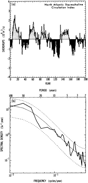
FIGURE 3
(a) Time series of the annual mean intensity of the index of the meridional overturning in the North Atlantic. Units are sverdrups. (The long-term mean of 18.28 sverdrups has been removed from the time series prior to plotting.) Heavy, solid line is a smoothed time series computed by applying a 13-point binomial filter to the annual mean data (approximately a 10-year low-pass filter). (b) Heavy, solid line denotes spectrum of the thermohaline circulation index time series shown in (a). Thin, solid line denotes the least-squares best fit of a theoretical red-noise spectrum to the spectrum of the THC. Dashed lines denote 95 percent confidence limits about the red noise spectrum. Note: The spectrum was computed by taking the Fourier transform of the autocovariance function, using a maximum of 50 lags and a Tukey window (Chatfield, 1989, Chapter 7). (From Delworth et al., 1993; reprinted with permission of the American Meteorological Society.)
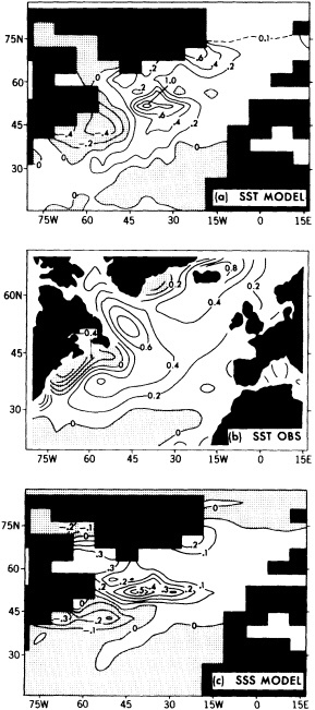
FIGURE 4
(a) Differences in annual mean model sea surface temperature between four decades with anomalously large thermohaline circulation index values and four decades with anomalously small thermohaline circulation index values. Units are °C. Values less than zero are stippled. (b) Difference in observed sea surface temperature between the periods 1950-1964 (warm period) and 1970-1984 (cold period). Units are °C. Values less than zero are stippled. (Adapted from Kushnir, 1994; reprinted with permission of the American Meteorological Society.) (c) Differences in annual mean model sea surface salinity, computed in the same manner as for Figure 4a. (From Delworth et al., 1993; reprinted with permission of the American Meteorological Society.)
subtracting the 1970-1984 mean (cold period) from the 1950-1964 mean (warm period). These 15-year periods were chosen on the basis of analyses of areal average SSTs in the North Atlantic (see Kushnir (1994) for details). There is a resemblance between the model and observational results, in terms of both the spatial pattern and the magnitude. It is tempting to speculate that the observed changes in SST may have arisen because of changes in the intensity of the THC in the North Atlantic. The pattern of model sea surface salinity (SSS) changes associated with fluctuations in the intensity of the thermohaline circulation, shown in Figure 4c, is somewhat similar to the pattern of model SST changes. Additional analyses have shown that the SST and SSS patterns in Figure 4 can be interpreted as the result of anomalous advection of the climatological mean SST and SSS distributions by the anomalous currents associated with variations in the THC. It should be noted that the pattern of model ocean temperature and salinity changes at 295 m depth (not shown) also resembles the observational results of Levitus (1989a), in which differences in ocean temperature and salinity were computed for two 5-year periods comprising 1955-1959 and 1970-1974.
The changes in surface air temperature associated with fluctuations in the intensity of the thermohaline circulation, computed in the same manner as for SST and SSS, are shown in Figure 5. The geographical extent of the surface
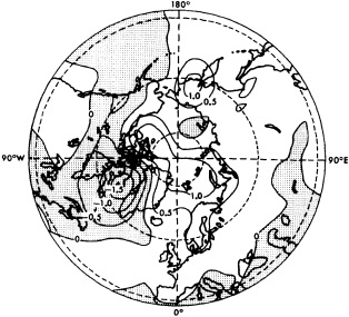
FIGURE 5
Differences in surface air temperature computed in a manner similar to that used for Figure 4a, except that only data from the months of December, January, and February was used. Values greater than 0.5 are densely stippled, values less than -0.5 are lightly stippled. A polar projection is used. Actual coastlines are used in the construction of this map in order to facilitate orientation. (From Delworth et al., 1993; reprinted with permission of the American Meteorological Society.)
air temperature changes is not restricted to the North Atlantic, but encompasses large regions of northern Europe and the Arctic. (Note that these surface air temperature results are from the winter season only.) Over the Arctic Ocean and its vicinity, surface air temperature changes are particularly large in winter. This seasonal dependence in the high latitudes results partially from changes in sea-ice thickness associated with changes in the intensity of the thermohaline circulation. When the THC is anomalously strong, the enhanced transport of heat into high latitudes results in a reduction of mean sea-ice cover (not shown), thereby permitting an enhanced heat flux from the ocean to the atmosphere during the winter months when the mean surface air temperatures are substantially lower than that of the ocean at high latitudes. During the summer, the mean surface air temperature over the Arctic Ocean is equal to or greater than the ocean temperature at high latitudes, and there is little or no heat flux from the model ocean to the atmosphere. However, the enhanced surface absorption of summer insolation due to the reduced coverage of sea ice also contributes to the reduction of sea ice thickness and the increase of surface air temperature in winter.
The above results highlight the potential importance to climate of such fluctuations in the thermohaline circulation over the North Atlantic, Europe, and the Arctic. These variations arise in the absence of any external forcing at this time scale.
Ocean Density Variations
It is desirable to examine in greater detail the spatial and temporal relationships between the irregular oscillations in the intensity of the thermohaline circulation and variations in the three-dimensional fields of salinity, temperature, and density. These relations are quantified by computing, at each grid point, linear regressions between the time series of temperature, salinity, and density versus the time series of the thermohaline circulation. The regressions were computed as:
where y(t) can be salinity, temperature, or density at each grid point, t is time, a is the slope of the regression line, x(t+ t) is the time series of the THC, t is the lag, and b is the intercept of the regression line. These regressions were computed at various lags in order to provide a three-dimensional picture of the evolution of the oceanic state as the thermohaline circulation fluctuates. Prior to the regression analyses, all time series were first detrended and filtered in order to effectively remove fluctuations with time scales less than approximately 10 years. The analyses were also performed without filtering; they yielded phase relationships similar to those described below. The slope of the regression line (referred to hereafter as the regression coefficient) esti-
mates the change in temperature, salinity, or density for a unit change in the intensity of the THC.
In order to provide a large-scale measure of conditions in the sinking region, the regression coefficients between density (ρ') and the thermohaline circulation were averaged vertically and horizontally over the sinking region. As can be seen in Figure 6, the density time series leads the thermohaline circulation time series by a few years, suggesting that fluctuations in density in the sinking region induce the fluctuations in the THC. In addition, the density term is
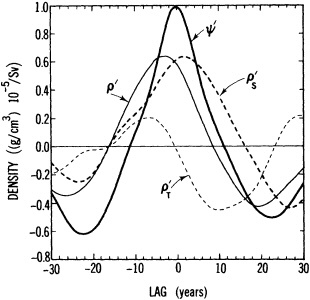
FIGURE 6
At each grid point at each model level, linear regression coefficients were computed between the time series of annual mean density, temperature, and salinity at that grid point versus the time series of the thermohaline circulation. The regression coefficients were computed using various lags in order to obtain an estimate of the temporal evolution of the three-dimensional fields of density, temperature, and salinity with respect to variations in the thermohaline circulation. These regression coefficients were then averaged vertically and horizontally over the sinking region of the North Atlantic (defined in text) and plotted as a function of lag in years. For example, the regression coefficients plotted at lag −5 (+ 5) years indicate conditions 5 years prior (subsequent) to a maximum in the thermohaline circulation. The heavy, solid line (ψ') denotes the regression coefficients of the THC index with itself (thus representing a ''typical" fluctuation). The thin, solid line (ρ') represents the regression coefficients between density and the THC index. The dashed line (ρ'S) denotes the regression coefficients for the density changes attributable solely to changes in salinity versus the THC index, while the dotted line (ρ'T) represents the regression coefficients for the density changes attributable solely to changes in temperature versus the THC index. Note that ρ'T is inversely related to temperature, whereas ρ'S is proportional to salinity. The units for ρ', ρ'T, and ρ'S are (g/cm3) 10−5/Sv. (From Delworth et al., 1993; reprinted with permission of the American Meteorological Society.)

FIGURE 7
Latitude by depth cross-section in the Atlantic basin of the zonal mean of the regression coefficients between the time series of density and the thermohaline circulation. The regression coefficients are computed at lag −3 years, indicating that the density values at year (n − 3) are correlated with values of the THC index at year n. This lag corresponds to the phase with the maximum vertically averaged density perturbation in the sinking region. Units are (g/cm3) x 10−5/Sv. Values less than zero are stippled. This cross-section can be interpreted as the anomaly density structure three years prior to a maximum in the thermohaline circulation. (From Delworth et al., 1993; reprinted with permission of the American Meteorological Society.)
decomposed into individual contributions from temperature and salinity anomalies, and the regression coefficients between these two terms and the THC are also plotted. This figure indicates that density fluctuations attributable to salinity anomalies (ρ'S) are almost in phase with, but slightly behind, the thermohaline circulation, whereas density fluctuations attributable to temperature anomalies (ρ'T) lead the thermohaline circulation by approximately 90° in phase. The sum of the effects of temperature and salinity anomalies results in a density time series that leads the thermohaline circulation by several years, as indicated in this figure. The phase differences between ρ'S and ρ'T shown in Figure 6 are important to the quasi-oscillatory nature of the fluctuations.
Temperature-induced density anomalies (ρ'T) serve as a negative feedback on the fluctuations of the THC. The largest negative ρ'T values (corresponding to the warmest vertically averaged temperatures) occur after the maximum in the THC, thereby reducing the mean density in the sinking region, and thus weakening the intensity of the THC. In contrast, the largest positive values of ρ'T occur before the maximum in the THC, thereby increasing the mean density in the sinking region and enhancing the intensity of the THC. Thus, temperature-induced density anomalies play and important role in these fluctuations.
To examine the latitude-depth distribution of the density
anomalies, the zonal means of the linear regression coefficients between density and the thermohaline circulation are shown in Figure 7. The lag chosen (˜3 years) corresponds to the time when the vertically averaged density anomaly in the sinking region is close to its maximum. This figure shows that, in the sinking region, positive density anomalies extend very deep, indicating the downward penetration of positive salinity anomalies. Note also the smaller negative density anomalies to the south of the sinking region. The distribution of the density anomalies described above forms a solenoidal field that intensifies the THC. As previously shown in Figure 6, the temporal variations of the vertically averaged density field in the sinking region precede the variations in the thermohaline circulation's intensity, implying that the former drives the latter.
A map of the regression coefficients between the time series of the near-surface density anomalies and the THC is shown in Figure 8. The largest density anomalies occur in the vicinity of the Labrador Sea and south of Greenland, with smaller values in the Greenland and Norwegian seas. Thus, the fluctuations of the model THC at this time scale appear to be related primarily to convection in the Labrador Sea and in the region south of Greenland. Variations in the near-surface currents associated with fluctuations in the THC support this conclusion. Shown in Figure 9 are the regression coefficients between surface currents and the THC. At each grid point, regression coefficients are computed between the meridional component of the surface currents and the THC, as well as between the zonal component of the currents and the THC. These regression coefficients are then plotted in vector form in the figure, so that the length of an arrow in the zonal (meridional) direction indicates the magnitude of the coefficient. Note that the current changes associated with fluctuations in the THC are
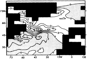
FIGURE 8
Regression coefficients of surface density versus the time series of the intensity of the thermohaline circulation. Regressions were computed with zero lag. Values less than zero are stippled. Units are (g/cm3) × 10-5/Sv. (From Delworth et al., 1993; reprinted with permission of the American Meteorological Society.)
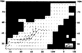
FIGURE 9
Regression coefficients between surface currents in the ocean and the intensity of the thermohaline circulation. Regressions were computed with zero lag. At each grid point, regression coefficients were computed between the zonal component of the current and the THC, as well as between the meridional component of the current and the THC. These regression coefficients were then plotted at each grid point in vector form, in such a way that the length of the arrow in the zonal (meridional) direction denotes the magnitude of the regression coefficients between the zonal (meridional) component of the current and the THC. The vector flow field shown in this figure may be interpreted as the change in surface currents associated with a unit increase in the intensity of the thermohaline circulation. Scaling and units are indicated by the arrow in the lower right-hand corner. (After Delworth et al., 1993; reprinted with permission of the American Meteorological Society.)
primarily confined to the western North Atlantic, scarcely affecting the Greenland and Norwegian seas. These changes in the current structure are not limited to the surface, but are found throughout the top 1 km.
The fluctuations of temperature and salinity in the sinking region, which determine the density variations and thus the intensity of the THC, are themselves generated by variations in the currents associated with fluctuations in the intensity of the THC. Budget analyses of the vertically averaged water column in the sinking region have demonstrated that the most important factors governing the heat and salt budgets for the sinking region appear to be the horizontal transports of heat and salt into the sinking region from that portion of the Atlantic that is south of the sinking region (for the heat budget, the surface flux is also important). These budget analyses have demonstrated that in addition to transport of heat and salt by the zonal mean meridional overturning, there are substantial transports of heat and salt into the sinking region by the horizontal gyre component of the flows. (Here, the horizontal gyre component of the flow is defined at each grid point as the departure of the meridional flow from the zonal mean meridional flow.) The phase of the gyre transport appears to precede the phase of the transport by the zonal mean meridional flow, suggesting
an important role for variations in the gyre transports in the model. Thus, these variations in the transport by the horizontal gyre component of the flow are an integral component of the THC fluctuations.
SUMMARY AND DISCUSSION
It has been shown that an irregular oscillation of the thermohaline circulation in the North Atlantic ocean appears in a coupled ocean-atmosphere model. This oscillation, which has a time scale of approximately 40 to 50 years, appears to be driven by density anomalies in the sinking region of the North Atlantic ocean combined with much smaller density anomalies of opposite sign in the broad, rising region. These density variations are in turn induced by fluctuations of the thermohaline circulation itself. Although it has not been confirmed here, one can speculate that the oscillation is triggered by nearly random surface-buoyancy forcing of heat and water fluxes.
Sea surface temperature fluctuations associated with the variations in the thermohaline circulation have a spatial pattern that bears an encouraging resemblance to a pattern of observed interdecadal variability (Kushnir, 1994). The SST anomalies induce surface air temperature anomalies of substantial magnitude over the North Atlantic, northern Europe, and the Arctic. The interdecadal time scale of this variability points out the potential difficulty of distinguishing natural variability of the coupled climate system from anthropogenic climate change, which would be expected to occur on similar time scales. Bjerknes (1964) suggested that low-frequency changes in SST over the northern North Atlantic are associated with variations in the intensity of the thermohaline circulation. The coupled-model simulation illustrates a physically plausible mechanism for such a complex low-frequency air-sea interaction. All that can be concluded is that the model variability is broadly consistent with what little evidence is available. Future studies of both the instrumental record and proxy paleoclimatic data have the potential for producing new evidence to further constrain models of North Atlantic climatic variability.
Commentary on the Paper of Delworth et al.
STEPHEN E. ZEBIAK
Lamont-Doherty Earth Observatory
I read Dr. Delworth's paper with great interest. I think it is the only result of its kind that we have: a coupled GCM that is producing decadal-scale oscillations that are sufficiently like what we observe to warrant careful study and scrutiny.
The paper mostly presents diagnostics of the oscillation. It left me with my appetite whetted but feeling somewhat disappointed. I am sure that I speak for many of us in saying that we are very anxious for further diagnostics and attempts to understand what is going on. From what was presented, I still do not understand what the essential mechanisms of this oscillation are. For instance, Dr. Delworth indicated differences in phase between the temperature and salinity components in the density field, but I am not sure from what I saw today why we would expect those phase differences.
Let me note a few questions. The first is the obligatory question about flux correction. Given the choice between not making flux corrections and thus having a totally unphysical climatology, and making flux corrections in order to have something more realistic-looking to start with, I think the flux correction is the better of the two. But with a phenomenon like this you can look to see whether the structure and the amplitude of the flux corrections that you are putting into the model give you confidence that the model processes, as reflected in your means, are not likely to yield results that will not be physical or realizable in the real world.
Next, I was struck by the fact that the variance of the coupled model seems to be lower than that in nature for almost all frequencies across the entire spectrum. I am curious to hear why that should be true.
I also noted with interest that on the figure showing the spectrum of the thermohaline circulation the only peak outside the 95 percent confidence interval derived from a simple red-noise spectrum occurred at four years. Dr. Delworth's method of analysis precludes looking at that so far, but I wonder whether there is something there of interest.
The paper showed a broad-band frequency spectrum in the first 200 years, but it seemed to be favoring 40- to 50-year periods. When the integration was carried further, it looked as though it might be shifting. I wonder whether it would be robust if the model were run for, say, 5000 years. Would it disappear or turn into something else? From my own experience, I know that with ENSO models that are chaotic, it is possible to get a certain behavior for quite a long time that then turns into something else. I should be interested in hearing any additional results from longer running that might bear on this topic.
One very important question is the nature of the atmosphere-ocean interaction. For the oscillations you get.
in what ways are the atmosphere and the ocean coupled? We obviously have coupling from fresh-water fluxes, from heat fluxes, and from momentum fluxes, and it would be of great interest to figure out whether, say, the wind-driven part of the ocean circulation has anything to do with what happens, or whether the primary coupling takes place through fresh-water fluxes and heat fluxes alone.
The reductionist approach is one way to attack this. For instance, if the atmospheric model is run with just an ocean mixed layer, do you get a mode that has anything in common with this? Similarly, the ocean could be run with just the mean wind field and precipitation fields prescribed from the atmospheric model, so the only coupling would happen through the atmospheric boundary-layer fluxes. Experiments like this might help determine what aspects of the coupling among the many in the full coupled model are primary in this particular oscillation.
I have already alluded to the differences in the temperature and salinity parts of the density fluctuations. As the paper mentions, one hypothesis is that the fluctuations are driven by noise. Another possibility is that the coupling between the atmosphere and ocean is sufficient to generate those fluxes without noise.
Discussion
DELWORTH: Many of the issues you've raised are fundamental and not easily soluble. With regard to the flux corrections, you should look at the spatial pattern, see where they're largest, and make some assessment of their importance. They can indeed be said to affect low-frequency variability, since without them there would be no overturning at all, but we can only speculate how much.
Let me show you again the spectrum of the thermohaline index I defined over the first 200 years, my Figure 3. If you compute a spectrum based on 600 or 800 years, the diminution of variance at the very-low-frequency end becomes clearer, but still doesn't pass the 95 percent limit. I tend to view the spectrum as characterized by an area of broad-band enhanced variance; I wouldn't say it's periodic. I also don't feel that the peak at four years has any meaning.
You asked whether these fluctuations are robust as the integration continues. On an index for years 200 to 400 you can still see the oscillation, but on a somewhat longer time scale. You see similar fluctuations on the others, all the way out to 1000 years. It's an open question whether this variability would be maintained in an even longer integration.
The analyses I've done don't suggest any role for the wind-driven circulation in these fluctuations. There is a coupling in terms of the sensible and latent heat fluxes that does appear to play some role; these fluxes are affected by mean wind speed and by large-scale changes of surface pressure and wind. I should point out that Yochanan Kushnir has done similar analyses with COADS pressure data, and the model results don't correspond well with observations, so there is certainly room for experimentation. Incidentally, the temperature and salinity differences between the phases is very important, because temperature provides a strong negative feedback on the density in the sinking regions, tending to stabilize these fluctuations.
MOREL: Disregarding the gyre for the time being, would you characterize this change in the overturning as essentially internal to the Atlantic Basin, or as a global signature?
DELWORTH: The integration is global, and the various analyses were computed globally, but the variations are pretty much confined to the North Atlantic on this time scale.
LEVITUS: Have you tried to trace any of these temperature/ salinity anomalies throughout the model?
DELWORTH: I see it more as changing intensity of the circulation operating on the mean gradients to produce these anomalies than as an anomalous water mass propagating through the model.
DIAZ: Have you seen anything indicating an out-of-phase sea surface temperature relationship between the North and South Atlantic?
DELWORTH: I haven't looked for that. Defining the index the way I do steers the analyses toward the North Atlantic.
SARACHIK: In the simpler sector models of the forced ocean we find two types of variability, very-long-term and the advective shorter-period variability you show. Your flux correction basically stabilizes the long-term thermohaline circulation, I think, confining you to the latter type.
DELWORTH: Well, my time series suggest that there may also be a lower-frequency mode, though it's hard to see in a 1000-year integration.
ROOTH: Manabe and Stouffer's two-mode experiment showed that there are two thermohaline circulation modes in the model even with the flux corrections in place.
CANE: There's been a lot of interest in the oscillations, but actually your response looks like a red-noise process. You're getting all kinds of durations for these changes, which may in fact be correct. Also, when you were discussing the effects on the atmosphere you ended up talking about sea ice Can you amplify a little on what role it might have in the ocean circulation as well as its effect on the atmosphere?
DELWORTH: I was expecting sea ice to play a strong role by changing sea surface salinity, but I didn't find it in the model. I did see movement of sea ice out of the Arctic into the convective regions, but it was on a higher frequency—5- to 10-year time scales—than these thermohaline fluctuations. In fact, the sea ice is virtually in phase with the fluctuations. In this model, and on this time scale, the ice appears to be reacting to changes in circulation rather than shaping them.
DICKSON: The top of your north wall is at about 1600 or 1800 meters. If you raised that to 600 meters, which would reflect reality, would you be able to get a deep enough overturning circulation in the model?
BRYAN: This is a persistent problem with these models. If we had the wall that high, we would get no overflow at all. But when we bring it down we get too much entrainment over the wall. Given their narrowness, it may be impossible to resolve the currents in a model like this.
Model Studies of the Long-Term Behavior of ENSO
MARK A. CANE, STEPHEN E. ZEBIAK, AND YAN XUE1
ABSTRACT
The ENSO cycle is irregular. As a result, time series of ENSO indicators exhibit variability from decade to decade.
There are at least two plausible suggestions in the literature for this low-frequency variability. ENSO could be a low-order dynamical system with chaotic dynamics, or it could be that there is no aperiodicity inherent in ENSO but that the ENSO system is jiggled by the external noise generated by the rest of the climate system. A third possibility is that the low-frequency behavior of the ENSO cycle is driven by variations in some other part of the climate system. Although possible in principle, thus far this last possibility has little support from the data record or from model simulations.
We consider these possibilities within the framework of models that have produced long-term aperiodic simulations of ENSO-like variations. We argue that in the models, at least, the ENSO cycle results from low-order chaotic dynamics. Model results are used to explore the possibility of unequivocally distinguishing chaotic dynamics from truly random behavior, which is difficult to do in the far more limited records of observational data. We conclude that the 100 years of instrumental data are probably insufficient, but despite added difficulties in interpretation, the much longer time series from proxy records may suffice.
INTRODUCTION
It is a well-known and well-documented fact that the El Niño/Southern Oscillation (ENSO) cycle is irregular. The paper in this chapter by Rasmusson et al. (1995, henceforth RWR), enhances this documentation. There is variation in the amplitude of the extreme phases of the cycle—warm and cold events—and in the interval between events. There is variation in the evolution of events: no two cycles are exactly alike, and occasionally the Southern Oscillation signals in the west Pacific assert their independence from the El Niño sea surface temperature (SST) signatures in the east. Furthermore, it is well documented that ENSO has global concomitants and global consequences (RWR; Ropelewski and Halpert, 1987, 1989: Glantz et al., 1991). These, too, vary in time. Indian monsoon rainfall, for example, shows some variability at the approximately 4-year
time scale characteristic of the ENSO cycle, but also varies on a variety of other time scales.
What is the reason for the irregularities in the global ENSO cycle? Generically, possible causes may be classified into forcings external to the ENSO cycle and nonlinear chaotic dynamics internal to ENSO. Such a division implicitly assumes that "ENSO physics" is a subset that may be disentangled from the larger system. We return to this point below.
If the forcing is outside of the physical ocean-atmosphere system, then there is no difficulty in accepting it as "external." Two examples that have been suggested in the literature are volcanic eruptions (Handler, 1990) and solar activity (Anderson, 1989). These two seem to have some currency. There have been others, including underwater tectonic activity and the influence of biological productivity on the penetration of sunlight. Although the case for volcanic eruptions has been pressed forcefully, a careful reconsideration leaves it without evidentiary support (Nicholls, 1988). The case for solar activity is quite tentative and will not be considered further here.
Forcings within the physical climate system but external to ENSO may be divided into "base state," the terminology used by RWR, and "noise." By ''base state" forcings we mean changes in the large-scale, low-frequency, global background state in which the ENSO phenomena are embedded. RWR detect no coherent relationship between variations in ENSO and in the base-state parameters they consider. By "noise" we mean factors external to the ENSO process with time scales that are short compared with the dominant time scales of ENSO. Their effects on ENSO are quasi-random. For example, Schopf and Suarez (1988) suggest that incursions of synoptic-scale systems from higher latitudes into the tropical Pacific are responsible for the aperiodicity of El Niño (cf. Battisti, 1988).
An alternate hypothesis is that the aperiodicity is a consequence of nonlinear chaotic dynamics internal to the ENSO system of interactions. The concept of dynamical chaos is by now well known, the most celebrated example being the three-variable system of Lorenz (1963). ENSO participates in the global climate system, which has an enormous number of variables, so this hypothesis requires that a relatively low-order ENSO subsystem be distinct from the system as a whole. This is possible, even reasonable, because it is consistent with the generally successful current paradigm that accounts for the principal characteristics of ENSO (see below).
In this paper we speculate on these three possible causes of the variability of the ENSO cycle: variations in the base state, in the noise, and in the internal dynamics. Our principal tool in this investigation is a numerical model (Zebiak and Cane, 1987; henceforth ZC) that has been used to predict the ENSO cycle a year or more ahead and to simulate its long-term behavior. Ultimately, a theory for the causes of ENSO variability must be verified against real-world data. However, as the discussion of RWR vividly illustrates, the shortness of the instrumental record and the ambiguities of the proxy record make this problematical. Part of our purpose here is to use the model to explore how long or what sort of record might suffice to distinguish among alternatives.
The next section very briefly reviews the model and sketches a case for its suitability for the purpose at hand. We also sketch the theory for ENSO that is needed for what follows. The three sections that follow consider variability due to base state changes, noise, and chaotic dynamics. A discussion section concludes the paper.
THEORY AND MODEL
The ZC model is one of several that have led to a converging view of ENSO as an internal oscillation of the tropical Pacific ocean-atmosphere system (Zebiak and Cane, 1985; ZC; Schopf and Suarez, 1988; Hirst, 1988; Battisti, 1988; see Cane (1991) for a recent summary account). Although this view continues to be refined and elaborated (Chao and Philander, 1993; Jin and Neelin, 1992; Latif et al., 1993), it is fair to say that we now have a widely accepted paradigm for the generation and maintenance of the ENSO cycle.
The core of the paradigm is the two-way ocean-atmosphere interaction hypothesized by Bjerknes (1969). Briefly, the thermal contrast between the cold eastern equatorial Pacific and the western Pacific warm pool drives the easterly trades at the surface. The easterlies create the contrast by driving the upwelling and advection that make the eastern Pacific cold. Thus there is a positive feedback in this coupling. The same feedback in reverse gives the El Niño state: if the east warms, the trades relax, the east warms further, the relaxation of the trades increases, and so on.
What was lacking in Bjerknes' scenario was a mechanism for the cycle, the transition from one state to the other. The answer lies in equatorial ocean dynamics. When the east warms anomalously, the layer of warm water above the thermocline thickens. This excess must be compensated for by a deficit of warm water elsewhere in the basin. Equatorial dynamics dictates that it will be to the west, off the equator, in the form of equatorial Rossby wave packets. The Rossby waves propagate west until they encounter the boundary. There their mass deficit signal is reflected eastward in equatorial Kelvin waves. This signal thins the warm layer in the east and eventually brings the warm event to an end and initiates a cold phase. The phase of cold waters in the east is necessarily accompanied by a warming in the west, which will eventually work its way around to initiate a new warm phase. And so the cycle continues ad infinitum.
Certain features of this "delayed oscillator" paradigm are important to our discussion. The essential interactions
are of large scale and low frequency; the number of degrees of freedom in the ENSO cycle could well be quite small. Only the tropical Pacific is involved; the rest of the globe is assigned no role. Of course, this does not preclude ENSO influences on the entire climate system.
The ZC model, which we rely on in the present study, was built with the Bjerknes hypothesis in mind. It is a model for the interactions of the atmosphere and ocean in the tropical Pacific. Although simplified in many respects, it produces aperiodic interannual oscillations that have many features in common with observed oscillations. The same model has been used in largely successful forecasts a year and more in advance of ENSO (Cane et al., 1986; Barnett et al., 1988; Cane, 1991).
Both the atmospheric and oceanic components of the model describe perturbations about the mean climatological state, with the monthly climatology specified from observations (Rasmusson and Carpenter, 1982). The atmospheric dynamics take the form of the steady, linear shallow-water equations on an equatorial beta-plane, with the circulation forced by a heating anomaly that depends partly on local heating associated with SST anomalies and partly on the low-level moisture convergence. The latter effect is nonlinear because latent heating occurs only when the total wind field is convergent, and this is a function of the background mean convergence as well as the calculated anomalous convergence.
The ocean model is set up in a rectangular basin extending from 124°E to 80°W, and 29°N to 29°S. The dynamics begin with the shallow-water equations, but are modified by the addition of a shallow frictional layer of a constant 50-meter depth to allow for the intensification of wind-driven currents near the surface. The thermodynamics describe the evolution of temperature anomalies in the model surface layer. All terms, including nonlinear advection components, are retained. Finally, temperature anomalies below the base of the surface layer are parameterized in terms of vertical displacements of the model thermocline (identified with movements of the layer interface).
The next few figures, from Zebiak and Cane (1991), are intended to allow the interannual variability of the model to be compared with that of the observations, thereby (we hope) establishing its credibility for the purpose at hand. Figure 1 shows a time series of NINO3 (90°W to 150°W, 5°N to 5°S) averaged SST anomalies from a 1024-year run of the model. Inspection of this time series reveals a wide range of behavior: there are well-marked periods of large-amplitude, rather regular oscillations and other periods of more chaotic, smaller-amplitude variability. Also of note are the period of nearly 20 years with negligible anomalies (near year 500), and periods of similar length with anomalies of only one sign. The other indices of Figure 1 describe these properties quantitatively and were devised as follows. The 1024-year (monthly) time series was divided into 51
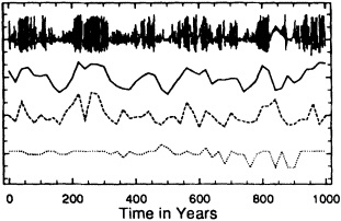
FIGURE 1
Time series of the NINO3-averaged SST anomaly from a 1024-year coupled-model simulation (top). Below are the three indices representing variance (heavy solid line), fraction of variance (dashed line), and dominant frequency (dotted line) for successive 24-year segments. (See text for definition of indices.) The heavy solid line indicates the overall intensity of ENSO activity for each 25-year period throughout the simulation. The dashed and dotted curves measure respectively the degree of regularity and the preferred period of El Niño cycles. Two regime types are evident: one in which strong and regular ENSO cycles of approximately 4-year periodicity persists, and another with weaker, more erratic behavior.
segments of 24 years' length (overlapping each other by 4 years). Within each segment, the mean, standard deviation, and power spectrum were computed. (A Welch window was applied prior to FFT calculation.) The spectral band with largest power was determined, as well as the fraction of total (interannual) variance contained in that band. Shown are the standard deviation, dominant frequency, and fraction-of-variance indices. The latter is a measure of the degree of regularity; nearly periodic oscillations result in large variance accompanying the dominant frequency, while chaotic variations result in variance spread among many bands. Two regimes are apparent: one with large variance, high regularity, and a dominant 4-year period; the other with lower variance, low regularity, and mixed periods. Thus, the indices provide a quantitative measure of the behavior patterns conspicuous in the original time series.
The distributions of the indices (among the 51 realizations) are shown in Figure 2. The standard deviation and fraction-of-variance distributions are notably broad, reflecting the distinct regimes. The favored frequency band centers on 4 years, but adjacent bands are also represented (3 to 6 years). For purposes of comparison, these same indices were computed from the single 18-year realization of observed SST anomalies between 1970 and 1987 (NOAA Climate Analysis Center analysis) and are indicated on the distribution plots. The observed values fall well within the range of the model-derived distributions, showing that, at least
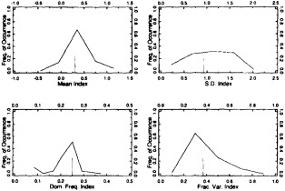
FIGURE 2
Distributions of mean sea-surface temperature (°C), standard deviation, dominant frequency (years–1), and fraction-of-variance indices from the 1024-year simulation. The values of each index computed from observed sea-surface temperature between 1970 and 1987 are indicated by vertical line segments.
for this period, the temporal characteristics of observed interannual variability are consistent with those of the model.
To examine the spatial structures, we computed empirical orthogonal functions (EOFs) of model fields on the basis of monthly values from the 1024-year simulation. Figure 3 shows the first four EOFs of SST anomalies. The first EOF, with 83 percent of the total variance, is clearly the mature El Niño signal. The others represent various phases of the life cycle of model warm and cold episodes. Corresponding EOFs derived from observed SST anomalies (1970 to 1987) are shown in Figure 4. Although there is correspondence between the patterns, two biases of the model are apparent: one underestimation of variability in the South American coastal region, and another in the vicinity of the dateline at the equator. Also, whereas the first four EOFs of the model fields contain 93 percent of the total variance, only 68 percent of the variance is accounted for in the observed fields. This partly reflects the absence of non-ENSO signals (that is, "noise") in the model fields. In addition, the model anomaly patterns are more consistent from event to event than in nature, as evidenced by the fact that the second EOF variance is a smaller fraction of the first for the model than in reality.
EFFECTS OF VARIATIONS IN BASE-STATE PARAMETERS
Because ZC is a perturbation model, the model framework allows a clean separation between ENSO and the base state. We may then consider the effect on model ENSO characteristics of changes in the model base state. Five parameters defining this state were chosen for a systematic study. They reflect the oceanic equivalent depth (Par 1), the sharpness (Par 2) and the amplitude (Par 3) of the mean thermocline, the strength of atmospheric heating associated with SST anomalies (Par 4), and the atmospheric friction (Par 5). A detailed treatment of these parameters can be found in ZC. For this study, each of the five parameters was allowed to assume each of three values—the standard one, a 5 percent decrease, and a 5 percent increase—in all possible permutations. This amounts to 35 or 243 simulations, each of which was run for 100 years (starting from the same initial conditions). The purpose of this study was to determine whether rather modest parameter changes could significantly change the model behavior, and if so, in what sense. Because of the large number of simulations, it is possible to assign statistical significance to the results, avoiding the uncertainties inherent in comparisons of individual realizations. After each 100-year simulation had been broken into four segments, the segments' characteristics were evaluated using the four indices defined above. To examine the individual effects of each parameter, the total set of results was grouped into three subsets corresponding to the three values of that parameter. Each of the subsets then contained 324 realizations. The cumulative distributions of each of the four indices were computed for each of the three subsets and then compared (Figure 5). In this form, the significance of differences in the distributions can be assessed using the Kolmogorov-Smirnov statistic (Conover, 1980). The 99 percent confidence interval derived in this manner is displayed in each distribution plot; there is only a 1 percent probability that two distributions (of size 324) differing by more than this amount represent the same process.
All five of the parameters produce significant changes in at least one of the indices, and the net effect of each parameter is unique. In the case of Par 1, increasing values produce smaller mean and standard deviation, and a tendency toward higher frequencies. Increasing Par 2 results only in decreasing the standard deviation on the high end (that is, decreasing the amplitude of the largest warm/cold events). Increasing Par 3 acts to increase the mean (marginally) and the standard deviation, while giving a more dominant 4-year period. For Par 4, the result of an increase is a larger mean and standard deviation, and a smaller fraction of variance (more irregular). Finally, increasing Par 5 leads to much reduced mean and standard deviation, a greater likelihood of dominant periods less than 4 years, and more regular oscillations. All of these effects are consistent and identifiable amid the background of natural variability, showing a genuine sensitivity to externally determined factors making up the background climate state. However, in most cases it would have been impossible to identify systematic changes without a large sample to work with: 324 realizations were used, whereas 100 years of data would yield only 5. Another consequence is that since many of the parameter settings yield distributions not significantly
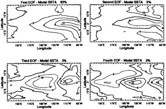
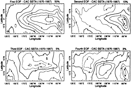

FIGURE 5
Cumulative distributions of mean SST, standard deviation, dominant frequency, and fraction-of-variance indices from the set of 243 simulations with variations in five model parameters. Across each row, the total set of results in each plot has been stratified according to the three distinct values of the indicated parameter. The heavy solid line represents the distribution for the subset with a 5 percent reduction of the parameter, the dashed line represents the subset with the standard value, and the dotted line represents the subset with a 5 percent increase. Also indicated in each plot (vertical bar) is the separation interval beyond which any pair of distributions may be considered distinct at the 99 percent level.
different from the order-of-100 years of instrumental data, a unique best-model fit to an observations model (i.e., a best set of parameter values) cannot be determined.
Figure 6 illustrates the issue. A number of 256-year time series with different parameter sets are shown. The variability within each series is more impressive than the differences between series. An obvious implication is that the effects of base-state changes of this magnitude are not detectable against the inherent natural variability of ENSO. Assuming that the model response to such changes is realistic, such base-state changes (e.g., due to greenhouse effects) would cause real changes in the climate system. However, we could not show them to be significant until they had persisted through tens of generations. Perhaps, then, it is fortunate that we are unaware of any compelling evidence for such changes in the recent past (cf. RWR). Any variations in such features as mean atmospheric temperature or decadally averaged tropical Pacific SST are more likely to be consequences than causes of ENSO variations.
INFLUENCE OF NOISE
Zebiak (1989) added to the ZC model a random wind forcing of a form intended to simulate observed intraseasonal variability in the tropical Pacific. That study demonstrated that this added noise did not alter the prediction skill of the model, the broader implication being that the intraseasonal variations have little effect on the predictability of ENSO at lead times up to two years. More relevant to present interests, the spectra presented there (his Figure 5) were virtually identical at periods longer than a year, indicating that the added noise made no difference in overall model behavior. Of course, this does not tell us the reasons for the ZC model's aperiodicity.
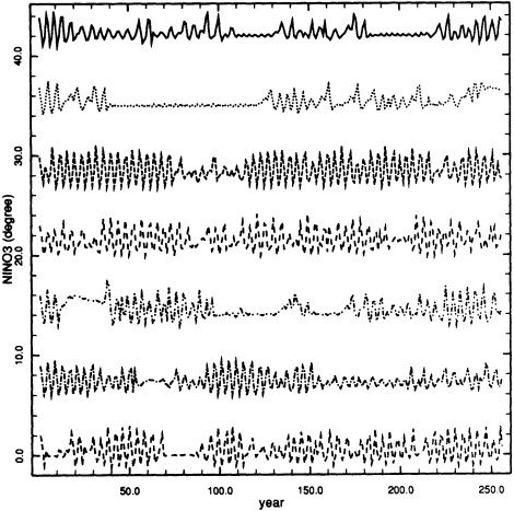
FIGURE 6
A set of 256-year-long time series of the NINO3 SST anomaly. Each is from a model run with different parameter settings; each began with the same initial conditions. Using a code where the nth digit is 0, 2, or 1 according to whether Par n is decreased by 5 percent, increased by 5 percent, or left at the standard value used in ZC, from top to bottom the cases are 02011, 02022, 11111. 12010, 12021, 12111, 12121. For example, the third curve is the standard case, while for the one above it Par I and Par 3 were decreased 5 percent while Par 2, Par 4, and Par 5 were increased 5 percent.
The time series of NINO3 from the model runs (Figures 1 and 6) appear to have characteristics associated with chaotic nonlinear dynamics: They are aperiodic and exhibit broad-band variability, with identifiable regimes persisting from a few years to more than a century. Nonetheless, it is not altogether straightforward to establish rigorously that these time series result from nonlinear dynamics.
Since the model is relatively simple, one might try an appeal on formal grounds: The model is nonlinear, and most of its variance is in an ENSO mode (e.g., Figure 3), so what other explanation could there be? However, not all of its variance is ENSO; there is other variability at smaller time and space scales. It may be argued that this acts as noise, preventing the model from settling into a periodic orbit. Battisti (1988) found his version of the ZC model to be periodic unless noise was added. Schopf and Suarez (1988) showed that in their model the irregular behavior disappeared when the atmospheric component of their model was replaced by a linear one. They attribute the difference to extratropical synoptic variability, which is effectively a source of noise for the ENSO dynamics.
However, the change in atmospheric model makes the interpretation ambiguous. Inevitably, it must alter the parameters influencing the ENSO physics, and it is well established that even small parameter changes may render an aperiodic model perfectly periodic (Jin and Neelin, 1992, and references therein). Such a change in model behavior can be induced, for example, by changes in any model parameters affecting the strength of the coupling between ocean and atmosphere (e.g., ZC; Münnich et al., 1991).
We will take the following approach to investigate the possibility that the model's irregular behavior is caused by noise. A long monthly time series (256 years) from a run of the fully nonlinear ZC model is best fit by a linear first-order autoregressive (AR) model:
where u is a vector of model state space variables, t is time in months, and e is the residual in the fit, which we model as white in time; i.e., e = Br, where r is a vector of independent random numbers uncorrelated in time. Our objective is to determine whether the behavior of the original nonlinear coupled model can be distinguished from that of this linear model driven by white noise.
The procedure for construction of the AR model is a variant of that described by Blumenthal (1991) and Blumenthal et al. (1992). Grid-point data from a long run of the ZC model are saved monthly. The original multivariate model grid-point time series are then transformed into a set of multivariate EOFs and associated time series (PCs). A truncated set of these principal components (PCs) constitutes the AR model state space u(t). In the results reported here, we retain the first 20 components, which capture over 95 percent of the variance in the model run. (Over 95 percent of the variance in the key model variables of surface wind, SST, and thermocline displacement is retained.) We note that this set can reconstruct the NINO3 index, an area average, with negligible error.
Given the time series u(t), the transition matrix A is found in the usual way as the best fit (in the least-squares sense) to the AR model equation (1). In recognition of the importance of the seasonal cycle, we elaborate the usual procedure by calculating a different A for each of the 12 monthly transitions (cf. Blumenthal, 1991). Once the A's have been determined, the 12 monthly values for B are calculated from the covariance of the residual time series e(t).
Figure 7 demonstrates the ability of the AR model to reproduce the behavior of the fully nonlinear coupled model in the short run—for a few years, at least. Clearly, this "best fit" model is a good fit indeed. We next want to see whether the long-term—interdecadal and beyond—behavior of the nonlinear ZC model can be distinguished from that of the AR model. If so, it would strongly suggest that ZC's long-term behavior is not well described as the response to a noise forcing of an essentially linear system. It is more likely a consequence of nonlinearities internal to the ENSO cycle itself.
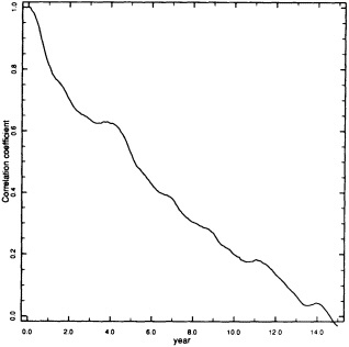
FIGURE 7
The correlation between the NINO3 index from the ZC model run and that obtained from the unforced linear AR model u(t+l) = Au(t) of Eq (1). The correlation is taken over the ensemble of AR model runs initialized from each of the monthly states in a 256-year ZC model run. Since the unforced AR model runs decay, the correlation must ultimately go to zero. That the correlation remains high for a few years demonstrates the ability of the AR model to reproduce the behavior of the fully nonlinear coupled model in the short run.
A NINO3 index time series typical of runs of the AR model is shown in Figure 8. The format is the same as in Figure 1. The similarities are more compelling than the differences, although there appears to be a discernible tendency for the regimes in the ZC run to persist longer. A comparison of power spectra of the NINO3 index from the ZC run and the AR run (Figures 9 and 10) adds to the
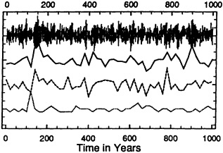
FIGURE 8
Time series of NINO3 SST anomaly from a 1024-year AR model run (top). The three indices below represent variance (heavy solid line), fraction of variance (dashed line), and dominant frequency (dotted line) for successive 24-year segments. Compare to Figure 1.
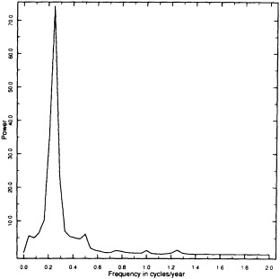
FIGURE 9
Power spectrum of the NINO3 SST anomaly from a run of the ZC nonlinear model. As described in the text, the 1024-year (monthly) time series was divided into 24-year-long segments, overlapping each other by 4 years, and a Welch window was applied. The spectrum shown is the average over all segments.
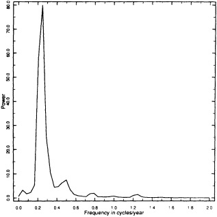
FIGURE 10
Power spectrum of the NINO3 SST anomaly from a typical 1024-year run of the AR model. See Figure 9.
impression that the two are quite similar. The AR model reproduces all the peaks at periods of a year and longer. (This was true of all the AR runs we made with different initial seeds for the random number generator, although, as should be expected, the runs differ slightly in the amplitudes of the peaks.) Figure 11 shows for the AR model the same distributions of regime indicators as were presented for the ZC model in Figure 2. The distribution of means is quite similar, as is the distribution of dominant frequencies, although there are somewhat more occurrences of longer
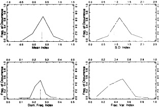
FIGURE 11
Distributions of mean SST, standard deviation, dominant frequency, and fraction-of-variance indices from a 194,560-year run of the AR model. (Compare Figure 2.) This run is a long enough sample to approximate closely the true distributions of the AR process (viz. the error bars on Figure 12).
periods for the ZC model. The AR model shows fewer instances of high or low standard deviations, that is, fewer 24-year periods either without events or dominated by strong ENSO events. Also, as the fractional variance index shows, the AR model tends not to have a single frequency dominating a 24-year period. While the ZC model clearly has periods with quite regular and quite large events as well as periods of rather little ENSO activity, the AR model exhibits a more uniform mix of such behavior within 24-year segments. The noise-driven linear model is less regime-like.
Applying the Kolmogorov-Smirnov test to these distributions shows this difference to be statistically significant, as is evident in Figure 12. In particular, the 1024-year (51-sample) ZC model run can be distinguished at the 98 percent level from the AR process by its differing standard-deviation and fractional-variance indices. The mean and the dominant frequency distributions are indistinguishable from those of an AR process. Note that if it were based on a run of only 100 years (5 samples), the ZC distributions would be indistinguishable from those of an AR process at the 98 percent level—or even at the 90 percent level. With 500 years (25 samples) the standard deviation distribution is just significant at the 90 percent level; even at this level the others are not distinguishable from the AR process.
Again, we are able to reach this conclusion because of the sufficiently large samples available to us with millennium-long simulations. With a 100-year record the distributions would have only 5 points, making it virtually impossible to establish statistical significance. Prospects for using long time series from paleo proxy data will be considered in the discussion section.
INTERNAL DYNAMICS
The analysis above builds a case for attributing the aperiodicity in the ZC model to nonlinear dynamics intrinsic to the ENSO cycle. Under the assumption of linear dynamics, it was shown to be unlikely that the regime-like behavior could be driven by noise. The possibility remains that non-linearities are essential and the noise is somehow important.
The ZC model could be doctored to eliminate all non-ENSO variability (e.g., by increasing frictional effects), but then any change in ENSO behavior is likely to have more to do with the alterations in model parameters than with the absence of noise. We take a different approach by showing that a still simpler model, one containing nothing but ENSO physics, can be aperiodic.
The model of Münnich et al. (1991, MCZ hereafter) is
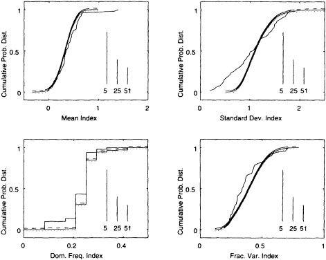
Figure 12
Cumulative probability distributions of mean SST, standard deviation, dominant frequency, and fraction of variance from a 1024-year run of the ZC model with standard parameters (solid curves), and the same distributions from the very long run (194,560 years) of the AR model. The 98 percent confidence limits on the AR model are given by the dashed and dotted lines. The vertical lines are the 98 percent confidence limits for 5, 25, and 51 samples, corresponding to runs of 100, 500, and 1024 years.
one of a number of conceptual models intended to illustrate and explore the Bjerknes cum delayed oscillator paradigm (Battisti and Hirst, 1989; Schopf and Suarez, 1988; for a recent elaboration and synthesis see Jin and Neelin, 1992). Cane et al. (1990) give a derivation and heuristic justification (also see Jin and Neelin, 1992). This will not be repeated here; instead we will stipulate that the arguments might fail to convince the determined skeptic that the MCZ model embodies the essence of the ZC model. We offer it as an analog, a demonstration that a prototype delayed-oscillator model is capable of aperiodic behavior.
The model equation is the solution for wind-forced motions described by the shallow-water equations on an equatorial beta plane. The wind forcing is purely zonal, is centered longitudinally in the model ocean basin, and has a fixed spatial form. The wind amplitude, A, depends solely on the thermocline height anomaly at the eastern end of the equator, h. The model may be reduced to the form of an iterated map (Eq. (6) of MCZ), which we write as
The only model variables are A and h. Time t is nondimensionalized by half the time it takes for an equatorial Kelvin wave to cross the basin. The α's and β's are numbers; in addition to n, they depend only on the meridional scale of the wind and the magnitude of the friction. In principle, the sums are from I to infinity, but convergence is rapid, so in practice they are cut off at N = 10.
In its primary nonlinear form, the model is closed by specifying a function A(h) for the dependence of wind amplitude on thermocline displacement. The function chosen (Eq. (9) and Figure 2 of MCZ), a linear piece inserted smoothly between two hyperbolic-tangent segments, is fashioned after the shape of the tropical thermocline.
The slope of A(h) at h = 0 is a measure of the strength of the coupling between atmosphere and ocean. Figure 13 illustrates the change of behavior as this coupling strength κ is increased. For very small κ the model decays. As it increases, there is a bifurcation resulting in regular oscillations with a period of around 2 years. For still larger κ there is a period doubling to a period of about 4 years. At κ = 2.16 the period triples, and for κ = 2.33 aperiodic behavior appears.
As discussed in MCZ, with this simplest version of the model it is a somewhat delicate matter to coax out aperiodic behavior. Either of two elaborations in the direction of greater realism makes this behavior quite robust. One is to add an annual cycle to κ, taking crude account of effects of the mean annual cycle in such factors as SST and wind speed. The other is to include in A the asymmetry between the warm (upper) and cold (lower) regions of the thermocline. Figure 14 is an example of the behavior obtained when both factors are included. The behavior is markedly irregular, although with a dominant period of around 4 years and noticeable power at 2 years. These characteristics occur for a wide range of parameter settings (although Figure 14 is one of the better specimens).
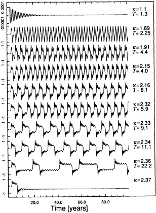
Figure 13
Time series of thermocline displacement h(t) as calculated from the iterated map (2) for various values of the coupling strength k. The function A(h) is symmetric about the center of the thermocline and does not include an annual cycle. (See text for details.) T, the average period in years, was determined from the output. (From Münnich et al., 1991; reprinted with permission of the American Meteorological Society.)
In this section we have recounted a model built as a paradigm for ENSO, stripped of any physics able to generate natural "noise" external to the ENSO cycle. In common with the real world and a number of numerical models, including ZC, it generates aperiodic behavior with a dominant period of about 4 years and some power at quasi-biennial periods. It adds to the argument that the most likely cause of the regime-like behavior of ENSO is nonlinear dynamics intrinsic to the ENSO cycle.
DISCUSSION
Is the natural variability of ENSO in the real world due to changes in the base state, forcing of the ENSO system
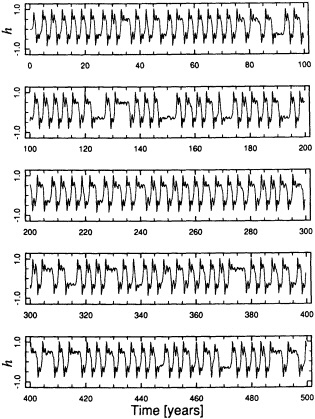
Figure 14
Time series of thermocline displacement h(t) as calculated from the iterated map (2) for an asymmetric thermocline shape, and an annual cycle modulating the strength of the coupling between ocean and atmosphere. (From Münnich et al., 1991; reprinted with permission of the American Meteorological Society.)
by climatic noise, or dynamics internal to the ENSO cycle itself? Can this hypothesis be verified for nature's ENSO?
The existence of models and theories for ENSO provides a valuable foundation for investigating its long-term variability. In this paper we have explored the possible causes for the irregularity of the ENSO cycle in a model, that of Zebiak and Cane (1987). The model is clearly sensitive to relatively small changes in its base state: Long model runs allowed us to make statistically reliable statements as to the effects of various parameter changes. However, the intrinsic variability within a run made with fixed parameters is quite often more marked than the difference between runs with different parameters (viz., Figure 6). Discerning systematic parameter effects typically requires far longer time series than the 100 years of instrumental records. We see no way to attribute any of the variability of the past 100 years to variations in the base state (cf. RWR).
It is also unlikely that we will be able to detect reliably the effect of greenhouse warming on ENSO in the near future. However, experience with models will allow the inference that changes in the base state bias the climate system so that certain ENSO characteristics (e.g., a more regular cycle) become more likely (cf. Zebiak and Cane, 1991).
We examined the possibility that natural noise, such as intrusions of mid-latitude synoptic systems, could force aperiodicity in the ENSO cycle. We concluded that this is a viable mechanism, but were able to show that the behavior of the ZC model could be distinguished from the most realistic noise-forced linear auto-regressive model we could construct. Again, achieving confidence in this conclusion required a model time series much longer than 100 years.
We were thus left with the presumption that the aperiodicity of the ZC model is due to chaotic nonlinear dynamics intrinsic to the model's ENSO cycle. This was bolstered by a consideration of a noise-free conceptual model (Münnich et al., 1991) of the Bjerknes-delayed oscillator paradigm. In common with the ZC model, it produced records dominated by an approximately 4-year cycle, but with power at quasi-biennial periods as well as interdecadal regime-like behavior.
According to Occam's Razor, these results recommend the following as a working hypothesis: The principal cause of all the variability associated with the ENSO cycle is low-order chaotic dynamics of ocean-atmosphere interactions within the tropical Pacific. ''All the variability" includes the basic quasi-quadrennial cycle, quasi-biennial variability (Rasmusson et al., 1990; Barnett, 1991; Ropelewski et al., 1992), and interdecadal variability (RWR). It includes all ENSO-related variability outside the tropical Pacific, such as that in the Indian monsoon rainfall record. This working hypothesis is not (yet) contradicted by any known facts. It is the minimum hypothesis needed to account for the observed global variability at all time scales associated with ENSO.
As noted early and often, the shortness of instrumental records makes it difficult—more likely impossible—to establish statistically significant answers. Certainly the sort of statistics we have examined in the model context would not allow it.
Our model results suggest that paleoclimatic proxy time series can be long enough to provide statistically significant answers. However, proxy data bring their own difficulties, stemming from the uncertainties in exactly what is being measured. Characteristics of a tree-ring series, or ice cores, or corals surely relate to large-scale climatic conditions, but it is equally certain that to some extent they also reflect local conditions. Moreover, if it is not clear precisely what combination of climatic variables they do measure, then the relationship between the proxy measurement and the output of a model will be problematic.
The issue may be rephrased to bring it closer to the present study. In testing whether a model is a suitable explanation for some observational data, the loss of predictability precludes reliance on anything as straightforward as a correlation. Whether it is due to noise or to intrinsic
nonlinear dynamics, we know a priori that the model will not closely reproduce long time behavior. Instead, we must look to see whether it reproduces more general characteristics, including statistical behavior. The underlying rationale for the relevant statistical tests is to check whether some measure obtained from two different samples could have been generated by the same random process. For example, we tested to see whether the distribution of standard deviations obtained from the nonlinear ZC model (Figure 2) might have been generated by a first-order auto-regressive process.
Now it is perfectly clear before we start that an ice-cap accumulation record, for example, is not generated by the same process as eastern equatorial Pacific SSTs. Both NINO3 SST and the Quelccaya ice cap are influenced by ENSO (Thompson et al., 1984) but are otherwise determined by quite different processes. It is not obviously possible to extract some statistic from records of the two that will reflect only the ENSO process, effectively "filtering out" everything else.
We calculated the same distributions as in Figure 2 for a 500-year record of accumulation in the Quelccaya ice cap (Thompson et al., 1984). As anticipated, even the most cursory inspection showed that the distributions were quite different from the NINO3 model results of Figure 2; accumulation is generated by a different process, and we failed to extract any usable characterization of the long-term behavior of ENSO.
Using an idea of Y. Zhao's, Zhao, Cane, and Zebiak have tried a different statistic. First, the time series are band-passed with a narrow filter centered at 4 years to reduce the non-ENSO "noise". Complex demodulation is then used to define an instantaneous amplitude and frequency. While for most of the time the frequency is almost constant (corresponding to periods near 4 years), it occasionally exhibits strong changes (>3.5 s). Figures 15 and 16 illustrate time series for the ice cap accumulation and for a ZC model run, respectively. The intervals between these transition times are termed "regime durations," and the distributions of these regime durations are taken as characterizing the underlying process. By testing for differences in the distributions, it is found that for a few parameter settings (e.g., the case 02011 shown in the top curve of Figure 6) the model series is not significantly different from the ice-cap accumulation record, while for others (e.g., the standard setting of ZC), it is. Perhaps the ice-cap proxy data can be used to distinguish among different candidate models, its shortcomings notwithstanding.
The statistic used to reach this conclusion, regime duration, is unfamiliar and indirect, requiring a multistep process to extract it from the time series. We advance it tentatively, a piece of evidence asking to be bolstered by further investigations and additional tests. We imagine that many readers find it unpersuasive. Be that as it may, concern with a particular test should not obscure the deeper issue.
There is now great interest in studying natural variability on time scales of decades and longer. Since the climate system contains both nonlinear chaotic subsystems and sources of what may be viewed as noise, even an impeccable model cannot reproduce a long natural time series. Since detailed predictions decades ahead are not possible, we must resort to statistical characteristics to check models and theories of long-term natural variability. The instrumental record can suggest many hypotheses, but is too short to allow rigorous tests. Time series long enough to contain many realizations of decadal variability can be found only in paleoclimatic proxy records. Because proxy records typically represent a nonlinear convolution of many climatic processes, both large-scale and local, novel methods are required to extract usable information. It will make the task easier to have available a number of simultaneous observational records suggesting by a clear hypothesis. And such records are essential; no matter how well a model reproduces short-term variations, only a test against long records can justify confidence in its long-term behavior.
ACKNOWLEDGMENTS
Valuable discussions with Zhao Yuechen and Yochanan Kushnir are gratefully acknowledged. Thanks to Virginia DiBlasi-Morris for her help in preparing the manuscript. This work was supported by grant NA16-RC-0432-01 from the National Oceanic and Atmospheric Administration's Office of Global Programs and grant ATM-89-21804 from the National Science Foundation. Lamont-Doherty Earth Observatory Contribution No. 4986.
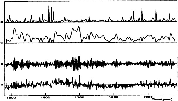
Figure 15
(a) Accumulation in the Quelccaya ice cap (courtesy of L. Thompson). (b) Band-passed accumulation record, filter centered at 4 years. Instantaneous (c) amplitude and (d) frequency, as obtained by complex demodulation: see text. (From an unpublished manuscript by Zhao, Cane, and Zebiak.)
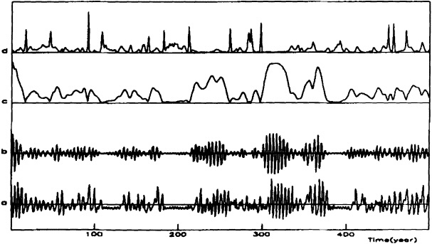
Figure 16
NINO3 SST anomaly from ZC model run 02011; see Figure 6. To be compared with the ice-cap accumulation record of Figure 15. (a) unfiltered record, (b) band-passed record, (c) instantaneous amplitude, and (d) instantaneous frequency. See Figure 15 and text. (From an unpublished manuscript by Zhao, Cane, and Zebiak.)
Commentary on the Paper of Cane et al.
S. GEORGE H. PHILANDER
Princeton University
Let me summarize. Julia Cole gave us an excellent talk and presented us with persuasive evidence that there is decadal variability in ENSO. Tomorrow morning Gene Rasmusson, using a completely different data set, will confirm those facts. Dr. Cane addresses the causes of the decadal variability of ENSO described by Drs. Cole and Rasmusson.
I thought his was a very clear presentation, and there is an excellent paper that accompanies it. I confess that I did not pay much attention to all the statistics in the paper; it seems to confirm the adage that statistics serves us in the same way that a lamppost serves a drunk: primarily for orientation rather than illumination. Those of you who are disoriented as regards the use of short-term records should by all means go through the paper. As regards illumination, I feel that the reason why ENSO is variable is still open to discussion. Dr. Cane considered three mechanisms: chaos, noise, and base-state modulation. He voted for chaos, invoking William of Occam.
The only substantive criticism I have of this paper concerns the discussion of a typical time series from the model. (See Figures 1 and 6 of Cane, Zebiak, and Xue above.) In these records there are actually two time scales, so that there are two issues to be addressed. Dr. Cane lumps them together. First, there are decades when the model behaves in a quasi-periodic manner, and there are other decades when nothing seems to happen, so one question is: Why is the time series non-stationary? A separate question is the following: When the model has quasi-periodic behavior, what causes the broad-band spectrum? In other words, why is the oscillation not perfectly periodic?
From simulations with other coupled ocean-atmosphere models we know that simulations of the Southern Oscillation can reproduce perfectly periodic oscillations unless "noise" is introduced. But if noise causes the aperiodicity, and we cannot predict noise, then why is it that we can predict El Niño? Tools (models) to do so exist, but I do not believe that we understand why El Niño is predictable.
A separate issue is the "non-stationarity" of the time series. Why is El Niño more prominent during some decades than others? Tropical oceanographers take a great deal for granted before they build their models. They assume that there is a thermocline and that its depth is given so that certain phase speeds for waves are also assumed. If they were to increase the depth of the thermocline and change the phase speeds and so on, they would be in a different regime altogether, possibly one without El Niño.
It seems to me that such changes probably involve the global thermohaline circulation, which determines the depth of the tropical thermocline. So it is quite possible that the tropical and extratropical oceanic circulations cannot be isolated from each other if the decadal variability in Dr. Cole's records is to be explained.
In summary, it seems to me that Dr. Cane's interesting study leaves some crucial questions unanswered. To attribute the variability in the model to chaos is a form of poetry. Even if it were chaos, surely there would still be something physically different in the system at different times. Exactly what changed the system from the one state to the other?
Discussion
CANE: I've just been thinking about the issue of statistics. It seems to me that the maturity of a subject is inversely related to the number of spectra shown when it's discussed. But we may have to fall back on statistics to make judgments about the models or mechanisms proposed as explanations for irregular behavior and long-term variability. How do we distinguish between internal chaotic dynamics and changes in background conditions like circulation? I can't really rule out changes in the base state, but it is incumbent on those who offer them as explanations to identify the particular change and a mechanism by which it operates. I have generated these series with models to demonstrate that in fact chaos could account for the results. William of Occam's principle is particularly appealing to those of us who don't like to multiply hypotheses.
SARACHIK: When you fitted the noise model to the nonlinear model it gave you a good fit. Why are you so sure noise models won't work?
CANE: The noise model is interesting; we fit a month-to-month transition and it can mimic the spectral peaks out through 4 years. But it seems to be incapable of giving you the lower-frequency variability—longer than the 4 years—exhibited by the other model.
LEVITUS: Does your rather sweeping generalization that the El Niño phenomenon is contained within the Pacific mean that we don't need to monitor the Pacific to understand heat flux and the role of the ocean as part of the earth's climate system?
CANE: No more than it means you need to monitor only the tropical Pacific. There are other modes of variability, of which at least a few have some sort of internal dynamic that gives them coherent characteristics over the time scales of interest here.
MYSAK: Ten or 12 years ago we did a statistical analysis correlating sea level, SST, and salinity in the northeast Pacific with fish population, weights, and so on. The dominant spectral peaks that emerged were about 5 or 6 years apart—not El Niño, not decadal. Have you any suggestion what they might be connected with?
PHILANDER: I think we're back to the lamppost: orientation only, remember.
MCGOWAN: I don't remember whether I pointed out on my time series of the California Current that zoöplankton showed a huge El Niño response in 1958-59 and 1982-83, though not to any of the other El Niños.
RIND: It seems to me that the various possible causes other than El Niño should leave evidence elsewhere that could be looked for. We should be combining our information on El Niño variations with observations taken elsewhere to look for correlations.
RASMUSSON: As you get more remote from what I'd call the core region, you may get responses only to the larger events.
TRENBERTH: I have the impression that your conclusions pertain mainly to a model that is still very idealized. Also, changes have been observed in the base state in the real world—for instance, the shift in the location of the South Pacific convergence zone over this century.
CANE: I don't see that base-state changes contradict my main thrust—namely, that everything seems to be caused in these tropical regions—and I'd like to see evidence that it's otherwise before we abandon this minimum hypothesis. As for the spectra, I admit that our model leaves out a lot of climate-system processes, but by adding noise we can generate broad-band spectra that will match Julie Cole's.
KARL: Did you limit yourself to a first-order autoregressive process? If so, why?
CANE: Yes, I fitted that because I used a complete state/space representation that captures all the variance in the model; it's a multivariant first-order process that mimics the equations we started from.
KARL: Was there any correlation in the noise left over?
KAROLY: If you used some sort of maximum-entropy spectral estimation you'd get something like a high-order AR process. Mark, did you find that modifying your nonlinear model parameters to fit the ice-core records made any difference to the model's predictability characteristics on the 2-year time scale?
CANE: These runs started from the same initial conditions. They all go through a negative phase, in about the same way, and then start to diverge. For a small slice of the present they seem to be equally good, yet some of them have quite different behaviors for longer times. That's important to keep in mind if the plan is to develop a good model of the present so it can be used for exploring variability on all time scales.
TALLEY: George, when you said El Niño is predictable, what sort of time period did you have in mind?
PHILANDER: Over longer periods, such as months, it's predictable.
ROOTH: When you ran the model with different base states did you keep the base state consistent for each run? I should think it would be reasonably feasible to put in a strictly harmonic variation, which would make it easier to detect any response. The effects of external signals might exist even if the spectra can't always be recognized as distinct.
CANE: We didn't try to vary the base-state parameters. Maybe we could have excited some resonance, but we really had to limit the number of questions to keep it manageable.
ROOTH: I was thinking not so much about resonance as about any process with a nonlinear trigger phase. It would be sensitive to the superposition of two biases during that critical period, so that a background variable might influence the transitional effects quite substantially.
Secular Variability of the ENSO Cycle
EUGENE M. RASMUSSON1, XUELIANG WANG2, AND CHESTER F. ROPELEWSKI3
ABSTRACT
Secular changes can occur in both multi-decadal climate means and multi-decadal measures of variability. We have examined the secular variability of the ENSO cycle as revealed by commonly used indices, i.e., sea level pressure and sea surface temperature from the low-latitude core region of the oscillation. We view the low-frequency variations (periods longer than approximately 30 years) as a varying base state upon which the ENSO cycle is superimposed.
The following are the major findings of the analyses:
-
ENSO-cycle variance for 31-year periods has changed by a factor of two or more during the past century. The cycle was quite pronounced late in the nineteenth century, was relatively weak from 1920 to 1950, and has increased in intensity since then.
-
The century-scale variation in equatorial sea surface temperature was broadly similar to that in globally averaged sea surface temperature.
-
No obvious relationship could be detected between variations in the base-state parameters we analyzed (equatorial sea surface temperature and Pacific-Indian Ocean sector sea level pressure) and variations in the intensity of the ENSO cycle.
-
Regional statistics, such as those derived from the Quinn et al. ( 1987) compilation of strong and very strong El Niño events in Peru, cannot be considered a reliable index of basin-scale ENSO-cycle variability.
-
The century-scale variations in ENSO-cycle intensity broadly correspond to changes in all-India monsoon-season rainfall variability, to the modulation of the intensity of drought episodes over the U.S. Great Plains during the twentieth century. and, less clearly, to the century-scale variation in Sahel rainfall.
INTRODUCTION
Secular changes can occur in both multi-decadal climatic means and multi-decadal measures of variability. Changes in the mean indicate changes in the "base-state climate," while changes in variability are more closely related to changes in the frequency and/or intensity of droughts, heat waves, frost occurrence, and other features of year-to-year variability. Changes in variability may have a greater socioeconomic impact than changes in the mean—as, for example, the ENSO does.
Three basic questions come to mind in considering the secular variability of the El Niño/Southern Oscillation (ENSO) cycle:
-
What do we know about secular variability in the character of the ENSO cycle (amplitude, frequency, character of regional responses, etc.) on time scales of a few decades to a century?
-
Can the "observed" secular variations be related to changes in base-state climate parameters? On what time scales?
-
What are the climate processes associated with secular variability of the ENSO cycle?
Continuous time series spanning at least several hundred years, from enough points to resolve both temporal and spatial changes in the character of the cycle, are required to fully describe multi-decadal to century-scale ENSO variability. Since only a few instrument time series approach or exceed a century in length, this requirement is not remotely satisfied. Proxy reconstructions and historical records represent promising indirect sources of information for extending the instrument record, but few solid conclusions can yet be drawn from such proxy sources.
Returning to the first of the three questions posed earlier in this section, a partial picture of the general nature of ENSO-cycle variability during the past 100 to 150 years can be distilled from existing instrumental data. The primary objective of this paper is to provide such a description. Regarding the second question (relationship of secular variability to changes in base-state parameters), the observations do not provide the information required to quantify important base-state parameters such as stratification, depth of the thermocline, or strength of atmosphere/ocean coupling (Cane et al., 1995). Thus we simply compared secular changes in variability to secular changes in parameters that could be quantified by the observational data, i.e., equatorial sea surface temperature (SST) and sea level pressure (SLP) at selected stations in the Pacific-Indian Ocean sector of the tropics. The third question (processes involved) also cannot be effectively addressed with this limited data base. For insight into this question obtained from model simulations, see Cane et al. (1995) in this section.
Salient characteristics of the ENSO cycle are first described as background. The nature of the instrumental data base and proxy sources of information are then briefly reviewed. Evidence of secular variability derived from instrumental records is summarized; both the published results and the results from new analyses by the authors are reviewed. The new results and their implications are discussed, and conclusions are summarized.
ENSO CYCLE
After years of analysis of global correlation patterns in surface temperature, pressure, and precipitation, Sir Gilbert Walker (Walker, 1924) identified three large atmospheric oscillations: two "Northern Oscillations", centered in the North Atlantic and the North Pacific, and a larger, more pervasive "Southern Oscillation" (SO), whose centers of action are in the tropics. In a subsequent paper (Walker and Bliss, 1932), he characterized the SO as follows: "When pressure is high in the Pacific Ocean it tends to be low in the Indian Ocean from Africa to Australia; these conditions are associated with low temperatures in both these areas, and rainfall varies in the opposite direction to pressure. Conditions are related differently in winter and summer, and it is therefore necessary to examine separately the seasons of December to February and June to August."
Almost a half century later, Bjerknes (1969) described the link between above-normal SST and enhanced convection in the central equatorial Pacific. He further related the SST variations to Walker's SO, thus forging a link between the SO and SST anomalies, both positive and negative, over the entire span of the equatorial Pacific, including the El Niño phenomenon of the eastern equatorial Pacific. This system of coupled ocean/atmosphere interactions, and the associated global pattern of atmospheric teleconnections, has come to be known as the El Niño/Southern Oscillation cycle.
The meaning attached to phenomenological names such as the SO and El Niño has evolved over the years as meteorologists and oceanographers have attempted to adapt earlier descriptive terms to an evolving understanding of the nature and scope of these phenomena. This has sometimes moved full circle, first away from and then back to an earlier use of a term. The result has been a high degree of semantic anarchy in the literature (Aceituno, 1992) and a need to clearly define how terms are to be used.
The ENSO cycle is the dominant quasi-regular mode of global climate variability. Over an imprecisely defined "core region" that broadly corresponds to the area of the SO surface-pressure dipole referred to in the previously quoted Walker-Bliss definition, the SO is reflected as a broad-band (2-6 year) maximum in the variance spectra of pressure,
wind, air temperature, SST, and precipitation (Rasmusson et al., 1990; Ropelewski et al., 1992). A discussion of our present understanding of the processes which give rise to the ENSO cycle, as well as the atmospheric processes associated with remote teleconnections, are beyond the scope of this paper. Suffice it to say that the current consensus view is that the ENSO cycle is an internal oscillation of the tropical ocean-atmosphere system (Cane et al., 1995, in this section).
In this paper, El Niño is considered to be an unusual warming of the normally cool surface waters along the west coast of South America, primarily affecting the extreme eastern equatorial Pacific and the coastal regions of southern Ecuador and northern Peru. It is therefore viewed as one of the regional responses to the basin-scale ENSO-cycle rhythm described by Bjerknes (1969). The coastal El Niño warm episode typically runs its course in about a year (Rasmusson and Carpenter, 1982).
The phase and amplitude of the ENSO cycle is usually indexed by sea level pressure variations at stations representative of the SO pressure dipole or by SST anomalies in the central and eastern equatorial Pacific. In characterizing and indexing the ENSO cycle it is important to give due consideration to the seasonality of the anomaly fields, as emphasized by Walker and Bliss (1932). For example, basin-scale anomaly patterns in the low latitudes typically reach maximum amplitude during the last half of the year, and often change sign during the March-May period. Thus 12-month averages are more definitive if they span the May-April "ENSO year" rather than the calendar year (Wright et al., 1988).
DATA CONSIDERATIONS
Instrument Data
During the past four decades, the distribution of surface meteorological observations has been sufficient to permit the documentation of ENSO-cycle variations over the core region of the oscillation in considerable detail. Prior to that time, the data distribution, or at least that represented by the observations which have found their way into the readily accessible archives, is far less satisfactory. Little in the way of surface meteorological data from merchant ships is available during the two world wars. This deficiency is superimposed on a progressively poorer sampling in the ENSO core region from both merchant ships and land stations as one moves backwards into the late nineteenth century. Little reliable information can be distilled from the surface marine data prior to 1875, and no meteorological station time series are available from the Pacific prior to this date. In summary, a good deal of information on the variability of the ENSO cycle over the past 100-120 years can be obtained from instrument records. The record can be extended backward for a few more decades, albeit much less securely, using surface pressure data from Djakarta and a few Indian stations.
Historical Information
The behavior of the ENSO cycle prior to the last half of the nineteenth century can be deduced only from indirect evidence contained in historical records and paleoclimate reconstructions. The most notable historical data are the descriptive records from Peru that provide anecdotal evidence of El Niño-related rainfall anomalies, e.g., descriptions of severe or prolonged desert flooding, massive crop failures, disease, or insect infestations. Using this material and information from ships' logs, Quinn et al. (1987) compiled a chronology of El Niño occurrences since 1525.
In evaluating this chronology, one must remember that the regional El Niño anomalies, while related to ENSO-cycle swings, also exhibit a significant degree of independent behavior (Deser and Wallace, 1987), particularly in their intensity. The Quinn et al. El Niño chronology should therefore be viewed as related to, but not necessarily a good index of, the ENSO cycle itself. This caveat will be further dealt with in the Discussion section below.
Paleoclimate Reconstructions
Paleo-ENSO research has developed rapidly during the past decade and is now being pursued on a broad front. There are a large number of candidates for annual/seasonal-resolution proxy reconstructions. An overview of this subject can be found in Enfield (1992). High-resolution proxy variables are discussed by Baumgartner et al. (1989). A volume edited by Diaz and Markgraf (1992) presents a collection of paleo-ENSO papers. Ortlieb and Macharé (1992) have edited a volume of extended abstracts from the 1992 Paleo-ENSO International Symposium held in Lima, Peru. We discuss briefly three of the proxy candidates which may in due time yield important results: corals, tree rings, and ice cores.
The most logical candidates for ENSO proxy reconstructions are the ENSO-sensitive natural processes of the core region. Particularly promising are proxy records derived from the paleochemistry of coral reefs (Shen et al., 1992; Fairbanks et al., 1992). A variety of chemical tracers have been developed in corals from both sides of the equatorial Pacific Ocean for the purpose of establishing the variability of surface ocean parameters (SST, changes in insolation, upwelling, vertical mixing, precipitation, river discharge) on annual to century time scales. The paper by Cole et al. (1995) in this volume clearly illustrates the great potential for lengthening the record of ENSO-cycle variability from coral reconstructions.
Dendroclimatic reconstructions are of limited value in tropical regions because most tree species there do not form
distinct annual rings, and growth is less susceptible to the interannual variability of climate (Bradley and Jones, 1992). Proxy indices of remote ENSO teleconnections can be used as indices of the ENSO cycle if the teleconnection is well correlated with the core-region variations, and the correlation remains stable over decades and centuries. Estimates of the Southern Oscillation Index time series have been made from western North American-northern Mexican tree-ring chronologies (Lough and Fritts, 1989; Michaelsen, 1985), which index variations in winter rainfall that are modestly correlated with ENSO core-region variability.
Annual variations in the amount and chemical composition of precipitation accumulated on polar and alpine glaciers produce laminations that allow precise dating of these stratigraphic sequences over periods of centuries. Of particular relevance to the ENSO cycle are the cores from the Quelccaya ice cap in the southern Peruvian Andes (10°S) (Thompson, 1992; Baumgartner et al., 1989). Interannual variability in those ice cores is correlated with changes in the water level of Lake Titicaca (Thompson, 1992), which are in turn modestly correlated with the ENSO cycle.
In summary, rapid progress is being made in paleo-ENSO studies, but attempts to quantify ENSO-cycle variability from indirect indicators give rise to a variety of problems. Much of the research to date has been directed toward calibration and establishing the reliability of the proxy record. Each record has its own limitations, and calibration is often hindered by the lack of appropriate instrumental records. The most productive approach would seem to involve extensive intercomparison of proxy records and synthesis of information from a variety of sources.
ASPECTS OF THE INSTRUMENTAL RECORD
Literature Review
Following the work of Gilbert Walker in the 1920s and 1930s, there was much debate as to whether the SO was a physical reality or a statistical artifact. Troup (1965) examined data from the decades following Walker's study and found a continuation of the SO relationships. However, the correlations between station pairs were consistently weaker during the period 1921-1950 than they had been in Walker's earlier data. Berlage (1957) had previously observed that the SO was less well developed after 1920. Troup also found smaller variance in the 1921-1950 seasonal means, suggesting a decrease in the amplitude of the ENSO cycle by comparison with the earlier period.
Later studies have indicated an increase in the ENSO cycle variability after the 1921-1950 period. Trenberth and Shea (1987) comment that "the prominence of the SO has varied throughout this century. The SO was very strong from 1900-1920 at the time it was first documented and named. But it was not conspicuous again until after the later 1930s." Elliott and Angell (1988) reached a more or less similar conclusion. They found that seasonal correlations between eastern equatorial Pacific SST and SLP at a number of index stations have "been greatest since World War II, and were relatively high prior to World War I." They suggest that there have been changes in the character of the cycle: i.e., prior to World War I the pressure difference between the eastern Pacific and Darwin was more representative of the SO, but since World War II the pressure difference between the central Pacific and Darwin has better reflected the SO.
Further Analysis
The view of what constitutes "climate noise" and what distinguishes climate change from climate variability is largely dependent on the time scales of interest and the spectrum of climate variability. The conceptual framework for viewing this question is considerably simplified if the climate signal of interest exhibits a significant concentration of variance that rises well above the higher-frequency "climate noise" background and is also separated to some extent from concentrations of lower-frequency variance by a "spectral gap". The lower-frequency variability can then be thought of as reflecting changes in the climate "base state" on which the higher-frequency variability is superimposed. The ENSO signal satisfies this ideal situation reasonably well over large parts of the core region.
We have adopted this conceptual framework for further analysis of a number of core-region time series. Results from four of the mean monthly series will be described.
-
SST* (1874-1990). This is the mean SST over the area 0°-10°S, 90°-180°W; it serves as an index of ENSO-cycle SST variations over the equatorial Pacific. The time series was provided by H. Diaz (personal communication, 1992). Values are recorded back to 1854, but we found little information content in the series prior to 1874.
-
Bombay mean sea level pressure (1847-1990) from Parthsarathy et al. (1991). This time series serves as one index of variations in the Indian Ocean-west Pacific pole of the ENSO-cycle pressure seesaw.
-
Darwin mean SLP (1882-1988), from the NCAR surface data tape. This is a commonly used index of variations in the Indian Ocean-west Pacific pole of the ENSO-cycle pressure seesaw. Pressures prior to 1898 have been corrected by + 1 mb, as recommended by Trenberth and Shea (1987).
-
Tahiti mean SLP (1876-1988), which is commonly used as an index of variations in the southeast Pacific pole of the ENSO-cycle pressure seesaw. The record prior to 1935, assembled by Ropelewski and Jones (1987), has several gaps, ranging from 3 to 28 months. Elliott and Angell (1988) filled the gaps by interpolating from the Apia time series. We simply filled the gaps with long-term mean
-
monthly values, since Elliott and Angell found that this did not materially affect their results.
Singular Spectrum Analysis
We performed singular spectrum analysis (SSA) of these and other long time series from the ENSO core region to obtain a general picture of the degree to which various time series reveal a consistent picture of ENSO cycle variability. SSA is a variant of the principal component analysis applied to a time series. (See Vautard et al. (1992), Keppenne and Ghil (1992), and Vautard and Ghil (1989) for detailed discussions of the analysis technique and its practical application.) Like conventional EOF analysis of a two-dimensional array, SSA decomposes a time series into an ordered set of eigenvectors (EVs) and principal components (PCs). SSA EVs define the dominant empirical modes of variability in the time series. Each EV is a data-adaptive filter for a particular empirical mode from which the corresponding PC time series is obtained by passing this filter over the original time series. The number of points in the EV (filter) is the "window size" that determines the maximum period of fluctuations that can be resolved by SSA. The PCs provide a time series for each EV that reveals variations in the amplitude and intermittency of the individual modes. Following Rasmusson et al. (1990), a window size of 61 months was adapted that resolves the variations with periods less than 10 years, which includes ENSO-cycle variability.
Results of SSA analyses of Bombay SLP and SST* time series are now described. We chose Bombay rather than Darwin as our primary SLP index series because of its considerably greater length and the remarkable consistency of its ENSO signal with that in the SST* series. Figures 1 and 2 show the first five EVs for SST* and Bombay SLP. The leading EV for each of the two series primarily reflects low-frequency variations with periods longer than those that can be resolved by the 61-month window. EV I is essentially a running mean filter, although it also contains some ENSO-cycle variability for SST*. PC I (Figures 3 and 4) is quite similar for the two series for time scales longer than a decade, the main difference being the higher-frequency "ENSO embroidery" that appears in PC 1 for SST*.
EV 2 and EV 3 reflect the low-frequency component of ENSO variability identified by Rasmusson et al. (1990) in equatorial SST and zonal wind fields. The corresponding EVs for the two series are almost identical; they exhibit a period of around 44 to 48 months. Figures 5 and 6 show PC 2 for the two series. The correspondence is truly remarkable, with close-to-perfect correspondence of the major swings. This comparison provides convincing evidence of the consistency of both time series, and therefore of their validity as indices of ENSO-cycle variability since 1875. It also suggests that the Bombay SLP series can be used to extend the record back to 1847.
EVs generally appear in pairs, one even and one odd function. The EV 4-EV 5 pair reflects the near-biennial mode of ENSO variability described by Rasmusson et al. (1990) and Ropelewski et al. (1992). However, EV 4 also includes a trend that is the low-frequency, odd-function companion of the EV 1 running mean. The close correspondence between EVs and PCs continues through EV 7, and to a lesser extent through EV 10 (not shown).
SSA modes 2 through 7 reflect ENSO cycle variability and account for a total of 49 percent of the Bombay SLP variance and 65 percent of the SST* variance.
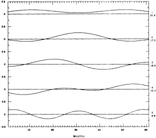
Figure 1
First five eigenvectors for SST* (see text). Percentage of variance explained by each eigenvector is shown on the right.
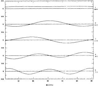
Figure 2
First five eigenvectors for Bombay SLP.
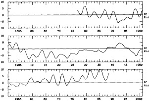
Figure 3
First principal component (PC1) for SST*.
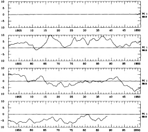
Figure 4
First principal component for Bombay SLP.
We also used the SSA analysis as an aid in the somewhat arbitrary choice of what constitutes the appropriate base state for each series, and what averaging period should be used to illustrate the nature of multi-decadal to century time scales of variability. Following the initial SSA analysis, the low-frequency component of variability was removed from the anomaly series by applying a multi-stage low-pass filter that has been extensively used in the field of astronomy (Zeng and Dong, 1986). It is basically a data-adaptive recursive filter. We first used the low-pass filter to obtain a base state that has a very sharp cutoff near periods of 30 years (Figure 7). Periods longer than 33 years are passed essentially unattenuated, while periods shorter than 27 years are almost entirely removed. We show filtered values to the ends of the series (Figure 8). The confidence limits for these end values progressively broaden as the end of the series is approached, but are tighter than those for a conventional linear filter. The general direction at the ends of the curves is more reliable than the absolute values.
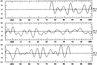
Figure 5
Second principal component (PC2) for SST*.
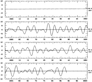
Figure 6
Second principal component for Bombay SLP.
SSA analyses were repeated after the series had been detrended by using this low-pass filter. The detrending removed EV 1 from each series, leaving the ENSO variability of each detrended series as the leading SSA modes—i.e., EV 2 of Figures 1 and 2 became EV 1 of the detrended series, EV 3 became EV 2, etc. We therefore judged this filter to be satisfactory for the purposes of this study, although further fine-tuning of the procedure for obtaining the base state may be desirable.
Base States
Figure 8 shows an example of the base-state curve for Bombay SLP, superimposed on the original time series. Figure 9 shows the base-state time series and 31-year mean-
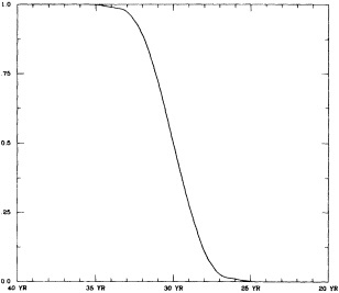
Figure 7
Response function for 30-year low-pass filter used in these analyses.
square departures (31MSD) for each of the four mean monthly time series. The 31-year mean-square departures are computed from the monthly values, i.e., ![]()
where Xi is a monthly value of the detrended series. For annual values, such as monsoon-season rainfall, the j index ranges from - 15 to 15. The 31-year averaging period is a compromise between resolution and stability. It should be firmly kept in mind that there are only three or four independent running-mean values and therefore relatively few degrees of freedom in the base state and 31MSD series.
We first discuss briefly the base-state curves. The Bombay SLP and SST* base-state curves are smoothed representations of PC 1 for each untrended series (compare with Figures 3 and 4). The SST data are uncorrected for biases that may have arisen as a result of the change from bucket to intake temperature measurements since World War II, but the broad-scale features of the SST* base-state curve are nevertheless similar to the global averages of SST, which we computed from several analyses of corrected SST data (Figure 10). The SST* base state shows an increase of more than 1°C since the 1910-to-1920 period, roughly twice that computed for the global average. The minor SST* maximum around 1940 and minimum around 1955 lead similar features in the global-average curves by around 15 years. The fall of SST* from the late nineteenth century to the minimum around 1915 is again around twice that computed for the global average. Thus, changes in tropical Pacific SST were generally of the same sense and larger than the century-scale changes in globally averaged SST.
Bombay exhibits a substantial century-time-scale trend toward lower pressure until 1955-1960, when values turned upward. Although of lesser amplitude, the same pattern is observed in the Madras, India, station pressure (not shown). The primary difference in the data from the two Indian stations occurs after the early 1970s, when the Madras upward trend flattens, while the upward trend at Bombay, as projected by the filter, continues to the end of the series.
There is no obvious relationship between the century-scale or decadal variations in SST* and Bombay SLP. Darwin does not show the high values prior to 1900 that are a feature of the Indian station data. However, the substantial correction applied to the Darwin pressures prior to 1898, together with the uncertainties of projecting the base-state curve to the beginning of the series (1882), leave the values prior to about 1910 in question. One could dismiss the Darwin data as biased, but the Tahiti base state also shows no high values during this period. Unfortunately, there are also uncertainties in the Tahiti data, since Ropelewski and Jones (1987) applied substantial corrections to the data prior to 1935.
After 1905, Darwin and Bombay base-state SLP curves follow a similar pattern of multi-decadal variations. Tahiti traces out the same pattern, lagging the opposite phase at Darwin by about 5 years. Except for the phase lag, the relationship between Darwin and Tahiti is similar to ENSO-cycle variations.
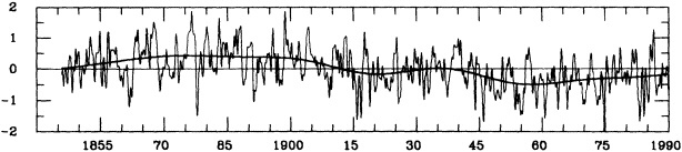
Figure 8
Base-state curve for Bombay SLP (heavy solid line). Lighter curve is the original time series after application of a light median filter (Rabiner et al., 1975) to eliminate isolated ''noise points." Units: millibars.
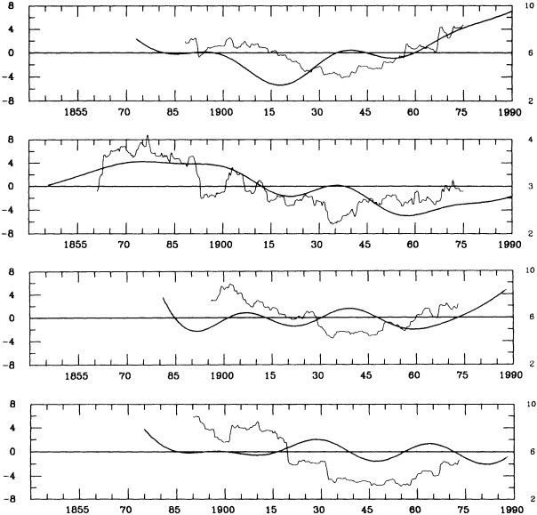
Figure 9
Time series of low-pass filtered base-state (solid curve) and 31-year mean-square departures for (top to bottom) SST*, Bombay SLP, Darwin SLP, and Tahiti LSP. Base-state units (left) are 10 -1°C or 10-1 mb; mean-square departure units (right) are 10-1(°C)2 or 10-1(mb)2.
Variability
The ENSO cycle is the dominant source of variability in the detrended time series. The first three EV pairs of the detrended series, which capture most of the ENSO-cycle variance, account for 68 percent, 75 percent, 79 percent, and 80 percent of the total Bombay, Tahiti, Darwin, and SST* variance, respectively.
The 31MSD series (Figure 9) exhibit a dominant century-scale variation with high variability late in the nineteenth century, the lowest variability during the third through fifth decades of the twentieth century, and increasing variability thereafter. The changes in the intensity of the ENSO cycle during the past century are substantial, with the 31-year mean maxima and minima differing by a factor of 2 or more.
The four 31MSD series of Figure 9 show a similar century-scale variation. The longer Bombay series shows that the period of high variability in the late nineteenth century probably extends back to around 1860. This is confirmed by the Madras station pressure series (not shown). The recovery from the twentieth-century minimum has been most pronounced in SST*, which has returned to the level observed prior to the sharp drop during the early 1890s. The question of whether this is at least partly due to inadequate sampling during the early decades needs to be investigated.
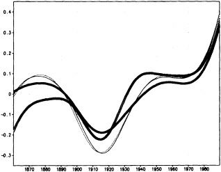
Figure 10
Time series of globally averaged SST. Heavy solid curve is obtained from the Comprehensive Ocean Atmosphere Data Set (COADS) (Woodruff et al., 1987) using optimum averaging (Vinnikov et al., 1990) with climatology as a first guess. The dashed curve is obtained from COADS using the box-averaging analysis technique (Bottomley et al., 1990), while the thin solid curve is obtained from COADS using optimum averaging with the previous month as the first guess. The open continuous dots are the curve obtained from the new SST data set and analyses described by Parker et al. (1995) in this volume. Units are °C.
The broadly similar character of the century-scale changes in SLP variability at the three stations shown suggests that the changes reflect primarily changes in the intensity of the ENSO cycle rather than shifts in one or both poles of the ENSO-cycle pressure seesaw. The 31MSD series for SLP shows greater irregularity than the SST* series. These irregularities are due to the contribution of individual large-amplitude swings, most notably that of 1877 to 1889. The presence of this feature maintained high 31MSD values until 1890, after which they dropped sharply as the 31MSD averaging window moved past this episode. To a great extent the great 1877-1878 ENSO cycle marked the climax of the late nineteenth-century period of high amplitude ENSO swings in SLP; it was less of a singular event in the SST* series, although this could be an artifact of inadequate sampling.
The ENSO swings during 1915 to 1920 also had a pronounced effect as they moved into and then out of the 31-year averaging window. The singular character of some of the ENSO-cycle swings and the marginal stability of the SLP 31MSD series suggest caution in drawing conclusions concerning any variability other than century scale.
The drop in variability at Tahiti after the turn of the century lags a similar feature in the other three series. This is also true for the subsequent minimum, and the recovery during the final decades is relatively small. The delay in the dropoff of variability can be attributed to the Tahiti ENSO swing of 1903-1907, which was much larger, in a relative sense, than that observed in the other series.
DISCUSSION
In the conceptual framework adopted for this study, ENSO-cycle variability that is concentrated in periods of two to six years is viewed as being superimposed on a varying base state that includes periods longer than around 30 years. The detrending of the time series by removal of the base state effectively "normalizes" the ENSO-cycle swings, so that they appear as more or less symmetric swings about a slowly changing base state. This picture of ENSO-cycle variability can be fundamentally different from what appears if the anomalies are simply computed as departures from long-term monthly means. Questions concerning the secular variability of the ENSO-cycle shift from "When and why were there periods when warm or cold "events'' predominated and were strong?" to "When and why did the amplitude or frequency of the cycle change?" The difference in perspective is illustrated by Figure 11, which shows the original and detrended anomaly series for SST*. An upward trend in SST* can be seen in the period since the late 1950s. From the original series, one might hypothesize a "jump" to a warmer state in 1977 (Trenberth, 1990). with a subsequent predominance of the ENSO warm phase, but there is little or no evidence of such a change in the ENSO cycle appearing in the detrended series.
We examined the question of whether the results of these analyses could be linked in any quantitative way with the previously noted coastal El Niño chronology of Quinn et al. (1987). Hocquenghem and Ortilieb (1992) have questioned the intensity classification of Quinn et al., as well as the reality of some of their earliest events. Their doubts arise from the fact that the coastal El Niño rains are usually localized in northern Peru and southern Ecuador, and within that region the rainfall distribution is highly variable from event to event. This makes it difficult to determine intensity from information at a single point. Since some of the events listed in the Quinn et al. chronology were identified on the basis of rainfall or flooding reports from the central and southern coastal regions of Peru, they may have been unrelated to El Niño occurrences.
Hocquenghem and Ortilieb (1992) conclude that "it is probably still untimely to use the Quinn et al. sequence of paleo-El Niño events as a solid basis for recurrence studies of the phenomenon". In contrast, Enfield and Cid (1991), while skeptical of the intensity classification for the weaker events, believe that recurrence statistics for the two strongest event categories, strong (S) and very strong (VS), are reliable. Their recurrence-interval analysis showed no indication of a multi-century Little Ice Age signal in the S and VS events. There were, however, significant variations in the recurrence interval on shorter (century) time scales.
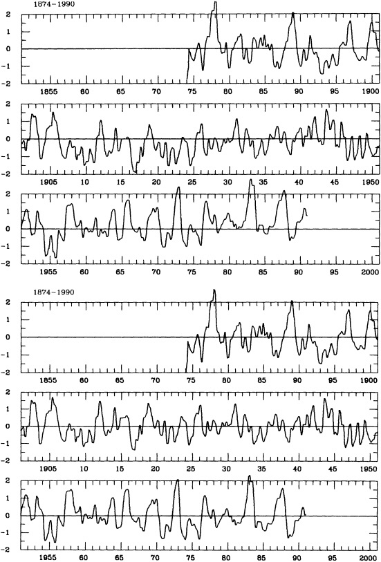
The problems inherent in the subjective classification of El Niño or ENSO-cycle intensity, even from instrumental data, become apparent when we compare our results with the chronology of Quinn et al. During the periods spanned by the Bombay SLP and SST* series, there were, respectively, 14 and 12 S and VS events in the Quinn et al. chronology. The average recurrence interval is therefore around a decade. This immediately raises questions regarding the stability of recurrence statistics for periods shorter than the century time scale.
Comparisons with the original SLP and SST* series were meaningless, since 11 of the 14 highest peaks in the Bombay series occurred during the period of high-base-state SLP prior to 1900, and 13 of the 14 occurred before 1920. For the SST* series, none of the 12 highest peaks occurred during the cold period between 1907-1956. When the detrended series was used instead, 20 of the positive Bombay anomaly peaks reached approximately 1 mb. Only 7 of the 14 S and VS events in the Quinn et al. chronology were included among these 20 peaks. For the SST* series, only 7 of the 12 S and VS events were included among the 13 largest positive swings. Nine of the 13 highest SST* peaks coincided with one of the 15 1 mb positive peaks in Bombay SLP during this period, indicating problems of classification even when instrumental records were compared. Comparisons were also made using the relatively smooth low-frequency ENSO-mode PCs instead of the more irregular detrended series. The level of agreement was about the same, although there were changes in the list of events exceeding a given threshold value.
The problems of subjective classification arise because of regional differences in the response from cycle to cycle and the relatively continuous distribution of amplitudes of ENSO-cycle swings. There are no obvious discontinuities in the distribution that could serve to separate classes, and slight irregularities from swing to swing and station to station often shift events from one class to another. The poor correspondence between the Quinn et al. chronology and the instrumental time series may arise for several reasons, among them the inherent difficulty of meaningful subjective classification, the poor agreement between the amplitude of ENSO-cycle swings and the amplitude of the regional El Niño response, and the difficulty of quantifying anecdotal information. Regardless of the reasons, we conclude from these simple comparisons that recurrence statistics derived from the Quinn et al. compilation of S and VS regional El Niño events cannot be considered a reliable index of basin-scale ENSO-cycle variability. Similar problems are likely to arise with any proxy record if ENSO fluctuations are classified by categories of intensity.
These analysis results provide no clear evidence of a relationship between base-state changes and changes in the statistics of the ENSO cycle. However, the data are admittedly inadequate for quantifying the base-state parameters of greatest interest (e.g., stratification, depth of the thermocline, strength of ocean-atmosphere coupling). Even if these parameters were available, the length of record might be far too short to reveal a relationship. For example, the ENSO cycle in the model used by Cane et al. (1995) for their study of the long-term behavior of the ENSO cycle results from low-order chaotic dynamics. It exhibits a pronounced regime-like behavior, and it would require a record many times the length of the observational time series to distinguish this regime-like behavior from changes caused by variations in the base state.
The question arises as to whether this pattern of ENSO-cycle secular variability over the past century can be related to secular variations in other aspects of global climate over the same period of time. In a recent review of large-scale precipitation variability, Rasmusson and Arkin (1993) cited three examples of pronounced secular variability in large-scale precipitation regimes: Indian monsoon-season rainfall, North American Great Plains drought, and Sahel rainfall. Figure 12 shows the base state and 31MSD series for all Indian monsoon-season rainfall (1871-1990) derived from the data published by Parthsarathy et al. (1991). The curves are similar to the 31-year running mean and variance shown in Rasmusson and Arkin (1993, Figure 19). The century-scale change in variability is broadly similar to that appearing in SST* and Bombay SLP. This is not surprising, since a significant correlation between Indian monsoon-season
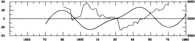
Figure 12
Time series of low-pass filtered base-state (solid curve) and 31-year mean-square departures (31MSD) for all-India monsoon-season (June-Sept.) rainfall. Base-state units (left) are mm, 31-year mean departure units (right) are mm2.
rainfall and the SO has been well documented (e.g., Walker (1924), Shukla and Paolino (1983)).
Folland et al. (1991) have shown a correspondence between the twentieth-century variation in Sahel rainfall (Nicholson, 1985) and a pattern of SST variability that appears as the third global EOF of SST. The EOF3 coefficient time series and the rainfall values show a large amount of annual- and decadal-scale variability, but both exhibit a pronounced century-scale variation that has a vague similarity to the century-scale changes in the ENSO-cycle variability, particularity the rapid changes after 1960 in the SST* and Sahel rainfall series. The EOF3 coefficients imply an increase in tropical Pacific SST after the mid-1940s, and while this represents only a small part of the total SST variability, it is of the same sign as the trend in the SST* base state.
Finally, the time series of the percentage of the U.S. Great Plains experiencing severe or extreme drought (Figure 13) shows a dominant interdecadal pattern of variability (Rasmusson and Arkin, 1992). It also shows a pattern of increasingly intense drought episodes up to the great Dust Bowl droughts of the 1930s, followed by a decrease in intensity. This suggests a modulation of the interdecadal fluctuations on the century time scale, with the more severe drought epochs corresponding to the period of low ENSO-cycle variability.
It is of course hazardous to even suggest relationships on the basis of a single realization of a "cycle." We are primarily calling attention to these "coincidences" as an area perhaps deserving of further investigation.
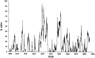
Figure 13
Area of U.S. Great Plains covered by severe and extreme drought. Data through March 1991. (Figure courtesy of the National Climatic Data Center, Asheville, N.C.)
CONCLUSIONS
Because of the global-scale coherence of the ENSO signal, considerable information on ENSO-cycle variability over the past 100 to 150 years can be extracted from a small number of long instrumental time series available from the core region of the oscillation. The results from earlier studies have been extended using SLP data from Bombay, Darwin, and Tahiti, and a time series of SST averaged over the central and eastern equatorial Pacific. The major conclusions from these and earlier analyses can be summarized as follows.
-
ENSO-cycle variance for 31-year periods has changed by a factor of two or more during the past century. The cycle was quite pronounced late in the nineteenth century, was relatively weak between 1920 to 1950, and has increased in intensity since then.
-
The century-scale variation in equatorial Pacific SST was broadly similar to that in globally averaged SST.
-
No obvious relationship could be detected between variations in the base-state parameters we analyzed (SST and SLP) and variations in the intensity of the ENSO cycle.
-
Regional recurrence statistics, such as those derived from the Quinn et al. (1987) compilation of strong and very strong El Niño events in Peru, cannot be considered a reliable index of basin-scale ENSO-cycle variability.
-
The century-scale variations in ENSO-cycle intensity broadly correspond to changes in all-India monsoon-season rainfall variability, to the modulation of the intensity of drought episodes over the U.S. Great Plains during the twentieth century, and, less clearly, to the century-scale variation in Sahel rainfall.
ACKNOWLEDGMENTS
This work was partially supported by the NOAA Equatorial Pacific Ocean Climate Studies. The senior author was partially supported by NSF Grant ATM-9013435. Data for Figure 10 were kindly provided by Thomas M. Smith of the NWS/NOAA Climate Analysis Center.
Commentary on the Paper of Rasmusson et al.
YOCHANAN KUSHNIR
Lamont-Doherty Earth Observatory
Dr. Rasmusson has just given us an example of the "extended bellybutton" approach to data analysis. He used an a priori knowledge of the pattern of variability in the data to identify key time series useful in monitoring the behavior of the system even during periods when data coverage was sparse. This method could be used with proxy data, as we saw yesterday in Julia Cole's talk. This is a model to follow when using sparse data in the study of decadal variability. This approach is preferable to looking at a single time series, since it contains information on the spatial structure of the phenomenon.
Here we have an advantage because ENSO is so coherent over space. Even in that vast area where we do not have enough observations, we can still find meaningful information simply because the phenomenon itself is so coherent over such a large part of the tropics.
I should like to say something about the "basic-state" idea discussed in the paper. The paper emphasizes that it is an arbitrary choice, a compromise in terms of the length of the data and the length of the ENSO cycle. It is indeed arbitrary; one of the things that we see, as Dr. Rasmusson mentioned, is that the basic state variables relate to one another in the same way that ENSO relates in different locations. This may mean that the basic state is just one of the low-frequency, maybe non-linear manifestations of the ENSO cycle itself, and thus it may not be the true basic state for the phenomenon we are dealing with.
The reference to a 30-year interval as the basic state is a helpful approach, however, at least for following the change in the main spectral peaks of ENSO, the four- to five-year cycle and the biennial cycle. In this way, he can actually follow changes in the variance of the more intense part of the phenomenon. Although it is hard to refer to the results as statistically significant, it is interesting to note that they are so coherent over space. They show, in a quantitative way, that there is a change in the variance of ENSO over time scales of a century or so.
The connection that is made at the end of the paper to other phenomena like monsoons, changes in droughts in North America, and the Sahel drought is very interesting and is food for thought in the future. It is obviously very hard to tie these phenomena together with only one cycle of each event. They may be in phase during one cycle and then drift out of phase, as is the case with two cycles slightly different in period. This is a delicate subject, and needless to say, we have to approach it very carefully.
Discussion
TRENBERTH: I'd like to go on record with a couple of comments on the very long time scales. I'm a little concerned about the skimpiness of the pre-1950 SST data, as well as its homogeneity. I'm also worried about the fact that at least one correction needs to be made for every one of the Indian stations. For example, detrending can remove some very real signals. On a century time scale this begins to call into question what you can really say.
RASMUSSON: If the detrending had removed a real signal, it would have induced jumps at the ends of the detrended period. However, it corresponded magnificently with Henry Diaz's data, which greatly increased my confidence in both time series.
DIAZ: Because of the large spatial coherence of the ENSO signal in that area, you can actually get pretty good signals back to about the 1877-1878 event.
RASMUSSON: I think that event was really the beginning of the turn-down of the early twentieth century. DIAZ: I'd like to see a study of the variations in the strength of the coupling between El Niño and Southern Oscillation events.
RASMUSSON: Yes. Quinn's long data set is very useful, but I don't think the categorization into strong, very strong, and so on is a good approach. The overlap with strong SST events is only half to two-thirds.
MYSAK: Gene, can you give us any insight into whether the slow interdecadal variations in the basic state in the Pacific are related to variations in the thermohaline circulation, as they appear to be in the Atlantic?
RASMUSSON: The correlations extend into the Atlantic, and particularly in the subtropics the Atlantic variability is definitely associated with the Pacific variability.
LEVITUS: That SOI/SST correlation seemed to be at an awfully low level. It's not clear to me that it could affect the thermohaline circulation at high latitudes.
RASMUSSON: That's for all the months; for the winter months the correlations get up to .5 or a little higher. Van Loon and Madden's pressure correlations extend out in exactly the same way. There's some sort of connection, and my guess is that it would affect things like the West Atlantic teleconnection pattern.
BRYAN: We've seen tremendous progress in proxy data sets. Gene, if we extend this research into the future, what would you like to see?
RASMUSSON: I'd like to see the coral people establish the long-term—300-to-500-year—character of the variations in what I call the core region, and then tie in with the tree-ring people at higher latitudes to see whether they could say anything about the stability of the teleconnnections. I am very much impressed with the coral data's potential for helping us reach a new level of understanding of secular variability.
KEELING: Julie's data show that same variance around 1920 to 1950. It seems to have hit a lot of different parameters. I think we need to keep an open mind about the possibility that something significant happened in that period.
RIND: Another unique thing about the 1920-to-1950 time frame is that there were no major volcanic eruptions.
CANE: We shouldn't forget that the variation during that period could also result from the internal dynamics of the system. There might be some way we could use the spatial patterns and multivariate changes to discriminate between what might be caused by some shift in the tropical Pacific and what might be caused by something else.
Decadal Climate Variations in the Pacific
KEVIN E. TRENBERTH AND JAMES W. HURRELL1
ABSTRACT
Considerable evidence has emerged of a substantial change in the North Pacific atmosphere and ocean lasting from about 1976 to 1988. Significant changes observed in the atmospheric circulation throughout the troposphere during that period show that a deeper, eastward-shifted Aleutian Low pressure system in the winter half-year advected warmer and moister air along the west coast of North America and into Alaska and colder air over the North Pacific. This advection caused substantial changes in sea surface temperatures over the North Pacific, as well as in coastal rainfall and streamflow, and in sea ice in the Bering Sea. Associated changes occurred in the surface wind stress, and, by inference, in the Sverdrup transport in the North Pacific Ocean. Changes in the monthly mean flow also imply substantial changes in the storm tracks and associated synoptic eddy activity, and in the sensible and latent heat fluxes at the ocean surface. In addition to the changes in the physical environment, large changes are found in the biology in the Northeast Pacific and in fish and other animal behavior.
It is suggested here that clues to possible causes of these changes lie in the close link between North Pacific changes on the decadal time scale and changes in the tropical Pacific and Indian Ocean, as well as the changes in frequency and intensity of El Niño versus La Niña events. A hypothesis is put forward outlining the tropical and extratropical relationships, which stresses the role of tropical forcing but includes important feedbacks in the extratropics that serve to emphasize the decadal more than interannual time scales. Whether the observed decadal variations are linked to "global warming" issues is an open question.
INTRODUCTION
Climate variations over the North Pacific and teleconnections downstream across North America have long been of interest; they have been particularly highlighted by the work of Namias (1959, 1963, 1969). Recently, considerable evidence has emerged of a substantial decade-long change in the North Pacific atmosphere and ocean that began about 1976. Changes in the atmospheric circulation throughout the troposphere at this time have been documented by Trenberth (1990; see Figure 1 below) and Nitta and Yamada (1989)
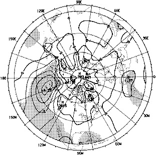
Figure 1
The difference between mean sea level pressures from 1977 to 1988 for November through March and those of 1924 to 1976 (mb). Stippling indicates statistical significance at 5 percent. (From Trenberth, 1990; published with permission of the American Meteorological Society.)
for the winter half-year. These changes were associated with changes in the surface wind stress, and, by inference, in the Sverdrup transport in the North Pacific Ocean (Trenberth, 1991) that have been directly measured in the Gulf of Alaska (Royer, 1989). Bakun (1990) has also noted changes in the alongshore wind stress off California that are probably related. Changes in the monthly mean flow also imply substantial changes in the storm tracks and associated synoptic eddy activity (e.g., Lau, 1988; Rogers and Raphael, 1992) and in the sensible and latent heat fluxes at the ocean surface (Cayan, 1992). The circulation changes were accompanied by changes in heat and moisture advection due to the quasi-stationary flow (see, e.g., Rogers and Raphael, 1992), so that there were substantial changes in the temperatures along the west coast of North America and in sea surface temperatures (SSTs) over the North Pacific (Trenberth, 1990), as well as in coastal rainfall and streamflow (Cayan and Peterson, 1989), and in sea ice in the Bering Sea (Manak and Mysak, 1987).
In addition to the changes in the physical environment, Venrick et al. (1987) observed associated large changes in the epipelagic ecosystem in the North Pacific, with increases in total chlorophyll in the water column and thus in phytoplankton. Mysak (1986) earlier noted that the changes in ocean currents and temperatures had altered the migration patterns of fish, in particular tuna and salmon, in the northeast Pacific (see also Hamilton, 1987). Ebbesmeyer et al. (1991) found that the "step in Pacific climate" in 1976 had a profound effect on 40 environmental variables. They contrasted the periods 1968 to 1975 with 1977 to 1984 and noted that climate-related changes were found not only in the above parameters, but in the behavior of geese, salmon, and crabs in the Northeast Pacific, and in mollusk abundance, salinity, and water temperature in Puget Sound. Also accompanying the changes in the Pacific was a higher incidence of cold outbreaks across the plains of North America, which ultimately led to major freezes affecting the Florida citrus crop (Rogers and Rohli, 1991).
The change in 1976 is but one of several large changes that have occurred in the North Pacific. As noted above, Namias has documented decadal-scale variations in the past, with coherent signals in the atmospheric circulation and in the SSTs, and with teleconnections downstream across North America (see also Douglas et al., 1982; Namias et al., 1988). The fairly sluggish response of the mid-latitude ocean to changes in the ocean forcing through the surface momentum and heat fluxes effectively serves as a low-pass filter and emphasizes the longer time scales. More recent studies throw further light on these aspects and on the physical links between the atmosphere and ocean in the North Pacific, and will be discussed below. New evidence has also emerged on the teleconnections downstream across North America, particularly those associated with the Pacific-North American (PNA) teleconnection pattern.
Possible causes of the changes were discussed by Trenberth (1990); he noted the close link between North Pacific changes on the decadal time scale and those in the tropical Pacific and Indian Ocean, as well as the changes in frequency and intensity of El Niño versus La Niña events. That paper expanded on the similar link noted during El Niño events by Bjerknes (1969). These aspects will be pursued and quantified further below.
The time series in Trenberth (1990) ceased after the northern winter of 1987-1988, and it is quite interesting to see what the subsequent evolution has been. Accordingly, in this paper, we update the time series and carry out some more comprehensive correlation analyses with surface temperature and SST analyses, and examine further the links with the tropical Pacific and the Southern Oscillation. The time scales of the main circulation anomaly patterns contributing to the decadal variation and the links with the tropics and teleconnections elsewhere are also of interest. A more complete version of this paper is presented in Trenberth and Hurrell (1994).
NORTH PACIFIC LARGE-SCALE OBSERVED TRENDS
In the North Pacific, a close association between SST anomalies and the atmospheric circulation has been well recognized. Changes in surface temperatures arise from
changes in temperature and moisture advection over the oceans by anomalous winds, and from the associated changes in surface fluxes and vertical mixing within the ocean. Anomalous northerly winds over the ocean are typically not only cold but also dry, so that large increases in surface fluxes of both sensible and latent heat into the atmosphere can be expected, which in turn cools the ocean. Convection and mechanical mixing in the ocean can spread those influences through considerable depth and may also entrain water from below the thermocline, giving the anomalies a finite lifetime (see, e.g., Frankignoul, 1985).
In the SSTs, a very distinctive pattern (cf. Figure 5) emerges as the dominant mode of an empirical orthogonal function (EOF) analysis (Davis, 1976; Lau and Nath, 1990) that is linked with a preferred mode of variability in winter in the Northern Hemisphere and is similar to the PNA teleconnection pattern of Wallace and Gutzler (1981). The PNA consists of four centers of action in the mid-tropospheric height field; they are of one sign near Hawaii and along the west coast of North America, and of opposite sign over the North Pacific and southeast United States. Wallace and Gutzler (1981) defined a PNA index using single-point values of 500 mb monthly mean geopotential height at each of the centers. This index does not appropriately weight the four centers of the PNA, and it is sensitive to errors in the analyses. Also, Northern Hemisphere upper-air analyses are available only after 1947. Wallace and Gutzler show that the surface signature of the PNA is mostly confined to the Pacific. An evaluation of sea level pressure charts (Trenberth and Paolino, 1980) shows them to be most reliable after 1924, and we therefore choose the area-weighted mean sea level pressure over the region 30°N to 65°N, 160°E to 140°W as a robust but simple measure of the circulation in the North Pacific. We refer to this as the NP index (for North Pacific). This is slightly smaller than the area used in Trenberth (1990), but corresponds better to the area participating in the decadal time-scale variations (see Figure 1). Trenberth (1990) noted that the correlation of the NP index with a PNA index based on all four PNA teleconnected centers at 700 and 500 mb is —0.92 for 1947 to 1987.
Figure 2 shows the NP index for all months of the year from 1924 through 1991. The first panel gives the total value of the index, and thus includes the mean annual cycle for three-month (seasonal) means that have been smoothed in time using a low-pass filter (with weights [1, 4, 8, 10, 8, 4, 1]/36, for which the half-power point is 11 years), which emphasizes the interdecadal fluctuations. The second panel shows the individual monthly anomalies (with the mean annual cycle removed) and is rather noisy, with the month-to-month variations prominent. The third panel shows the anomalies from the first panel, so that it is a smoothed version of the second panel, to show the most persistent anomalies. The figures emphasize that the period
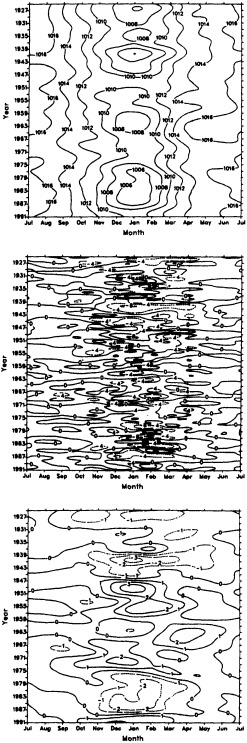
Figure 2
Time series of mean North Pacific sea level pressures averaged over 30°N to 65°N, 160°E to 140°W as a function of month and time. Top, total three-monthly mean values smoothed with a low-pass filter with seven weights ([1, 4, 8, 10. 8,4, 1]/36) across years to emphasize the decadal time scales in mb. Center, monthly mean anomalies in mb. Bottom, seasonal (three-monthly) mean anomalies smoothed with the low-pass filter in mb.
November through March corresponds to the wintertime regime, with low pressures in the Pacific, while for the rest of the year the Pacific tends to be dominated more by the subtropical anticyclone. Also, the main variability occurs only in November through March. Standard deviations of the monthly anomaly times series range from about 1 mb in the summer months to more than 4.5 mb in January and February. Values exceed 2.8 mb only from November through March. The variability from one month to the next in the same winter season stems in part from westward-propagating planetary-scale waves with a 20-day period (Branstator, 1987; Madden and Speth, 1989). Averaging over the five winter months removes much of this kind of noise.
Accordingly, Figures 3 and 4 show the NP time series for the five-month wintertime average. In Figure 3 the 1946 to 1991 time series is broken up to emphasize the regime from 1976 to 1988, while in Figure 4 the time series from 1925 is shown with the low-passed curve to reveal, without the arbitrariness of deciding on a start and end for the regime, just how unusual the 1977-to-1988 period is; the only previous time for which comparable values occurred was the much shorter interval from 1940 to 1941. Nevertheless, considerable interannual variability is present within the regime.
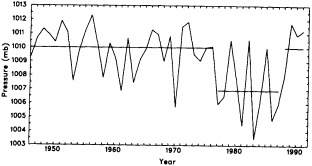
Figure 3
Time series of mean North Pacific sea level pressures averaged over 30°N to 65°N, 160°E to 140°W for the months November through March. Means for the combined periods 1946-to-1976 plus 1989-to-1991 and for 1977-to-1988 are indicated (1988 refers to the 1987-1988 winter).
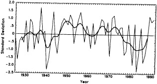
Figure 4
Time series of mean North Pacific sea level pressures for November through March, as in Figure 3, but beginning in 1925 and smoothed with the low-pass filter.
In the Aleutian Low from 1977 to 1988, for November through March, pressures were lower by 3.0 mb when averaged over the NP area of the North Pacific. Lower pressures were present individually in all five winter months and are highly statistically significant (Figure 1). No such change is present in any of the other months of the year (Figure 2). The wintertime changes correspond to the center of the low farther east and deeper on average by 4.3 mb for the five winter months, being deeper by 7 to 9 mb in January (Trenberth, 1991; see also Figure 1).
A climatology for surface wind stress based on the years 1980 to 1986 reveals changes in the North Pacific relative to a climatology based on ship data prior to 1977 that help confirm the reality of the sea level pressure changes (Trenberth, 1991), and so do analyses with independent data sets (Nitta and Yamada, 1989). Moreover, the associated changes in the curl of the wind stress and the corresponding Sverdrup transport in the ocean (Trenberth, 1991) over such a long period imply significant changes in the North Pacific Ocean currents.
The corresponding changes in surface temperatures are shown in Figure 5. The surface temperatures are taken from the updated Intergovernmental Panel on Climate Change (IPCC) data set (IPCC, 1990, 1992), which consists of land surface data from the University of East Anglia (Jones, 1988) blended with sea surface temperature data from the U.K. Meteorological Office (Bottomley et al., 1990; see also Trenberth et al., 1992). The surface temperature anomalies, expressed as departures from the 1951-to-1980 means, are shown for both the whole year and the five winter months November through March averaged over the 1977-to-1988 period. The temperature anomalies are strongly regional, and have both positive and negative signs. The 12-year period features very large North Pacific basin temperature anomalies, with warming of more than 1.5°C in Alaska and cooling of more than 0.5°C in the central North Pacific. The pattern in Figure 5 over the North Pacific is similar to the first EOF of SSTs (Davis, 1976; Lau and Nath, 1990). The annual mean anomaly clearly arises from the wintertime atmospheric anomaly, but over the North Pacific it is sufficiently persistent throughout the year that there is little difference between the annual and the five-month means. The wintertime pattern also reveals below-normal temperatures over the southeastern part of the United States, illustrating the PNA teleconnection. This is reflected in a higher-than-usual incidence of major freezes affecting the Florida citrus crop after 1977 (Rogers and Rohli, 1991).
The most compelling argument that the changes in sea level pressure are real is the physical consistency with the very large regional Pacific temperature anomalies for 1977
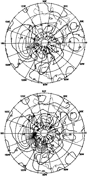
Figure 5
Twelve-year (1977-to- 1988) average surface temperature or sea surface temperature anomalies as departures from the 1951-to-1980 mean. Contours every 0.25°C. Shown are the annual mean anomalies (upper panel) and the anomalies for the five winter months (November to March). Negative values are dashed.
to 1988, shown in Figure 5. The warming over Alaska and along the west coast of North America, together with the cooling in the central and western North Pacific, would be expected to accompany a stronger Aleutian Low, because of thermal advection (Rogers and Raphael, 1992) and increased ocean mixing and changes in the surface fluxes (Cayan, 1992; Alexander, 1992a,b). The increased southward gradient flow in the eastern North Pacific, revealed by the pressure pattern in Figure 1, would bring warmer and moister air into Alaska and along the west coast of North America, while anomalous northerly winds would give rise to colder-than-normal conditions in the central and western North Pacific. Lower SSTs are a consequence of large sensible and latent heat fluxes into the atmosphere, combined with increased mixing in the ocean (Cayan, 1992). Cayan and Peterson (1989) found that increased stream flow in the coastal region of the northern Gulf of Alaska results from increased coastal rainfall associated with a deepened Aleutian Low and changes in the PNA.
To further illustrate the nature of the surface temperature changes associated with the NP index, Figure 6 shows the correlations for the November-to-March five-month average over 1935 to 1990, along with the corresponding departure pattern in degrees Celsius associated with a unit standard deviation departure of the NP index. For each grid point, ''seasonal" values were computed only when data existed for at least three of the five months defining the season. Correlations between variables were not computed if the two variables had fewer than 75 percent of the total number of seasons in common. Across the North Pacific and North American regions, these patterns show that the anomaly featured in Figure 5 is consistent with the whole record: Below-normal NP values are associated with below-normal temperatures over the North Pacific and southeast United States and above-normal surface temperatures along the West Coast, extending throughout Alaska and across most of Canada.
We have also investigated these relationships as a function of various lags. To objectively decide how much variance is explained by the correlations across an area, we have averaged the correlation coefficient squared for the region 140°E to 60°W, 30° to 65°N. The largest surface temperature variance explained by the NP index for this region occurs with NP leading by I to 2 months (r2 values with NP leading by 3, 2, 1, and 0 months are 0.15. 0.19, 0.20, and 0.16). The pattern is similar to that at zero lag, but the magnitude of the correlation coefficients increase by about 0.1 (to >0.6 over the North Pacific, and to < -0.7 over British Columbia).
The above results are consistent with those of Davis (1976). The link between SST in the North Pacific and the overlying atmospheric circulation has become well established. The main relationship seems to be one where the changes in the atmospheric circulation are responsible for the SST changes, as shown by simultaneous and lagged correlations, for instance (Davis, 1976, 1978; Lanzante, 1984; Wallace et al., 1990). Nevertheless, there is the strong expectation that extratropical SST anomalies also influence and may reinforce the atmospheric circulation (Kushnir and Lau, 1992).
Further confirmation of the link between temperatures and the atmospheric circulation comes from correlations between the NP index time series in Figure 2 and tempera
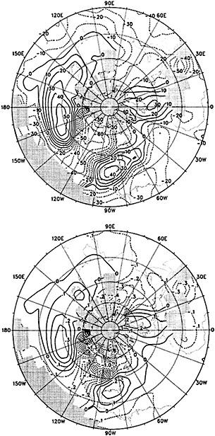
Figure 6
Correlations between the NP index and surface temperatures for 1935 to 1990 (upper panel) and the departure pattern corresponding to a unit standard deviation of NP. Negative values are dashed. The 5 percent significance level is 0.27. Shaded areas indicate insufficient data.
tures at 700 mb (Figure 7). The pattern of correlations reveals the four centers of the PNA. Over the Pacific and North America this pattern (with opposite sign) bears a striking resemblance to the actual surface temperature anomalies for 1977 to 1988 (Figure 5), including the cooling over the eastern part of North America. As shown in Figure 6, the latter is thus revealed as part of the overall teleconnection pattern. Over most of the domain, the 700 mb correla
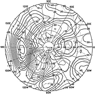
Figure 7
Correlations between the NP index in Figure 2 and 700 mb temperatures. Negative values are dashed. The 5 percent significance level is 0.30. Twenty percent of the variance is accounted for by the correlations over the 140°E to 60°W, 30°N to 65°N region.
tions are highest at zero lag. The exception is for the center over the southeastern United States, where correlations are 10 percent higher one month later, indicating that the development of the teleconnection downstream and the associated change in tracks of synoptic systems (see, e.g., Lau, 1988; Rogers and Rohli, 1991) may be somewhat delayed.
To complete the picture, Figure 8 shows the correlations of the NP index with the 500 mb height field, and the corresponding departure pattern. Once again, the PNA pattern emerges strongly, with all the PNA centers showing up, although the associated anomaly departure pattern clearly emphasizes the North Pacific.
CAUSES OF CHANGE IN THE NORTH PACIFIC
Examination of the possible causes of the various types of changes focuses attention on the association between the large-scale coherent climate variations and changes in atmospheric waves. The stationary planetary waves in the atmosphere are forced by orography and patterns of diabatic heating arising from the distribution of land and sea, both in the extratropics and in the tropics (see, e.g., Frankignoul, 1985). Therefore, in the Northern Hemisphere, changes in diabatic heating (for instance) can change the planetary waves and associated poleward heat fluxes. This mechanism does not operate in summer. In addition, when the temperature gradients on which the transients feed are altered
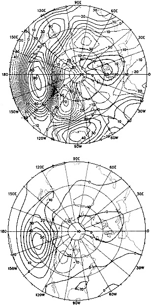
Figure 8
Correlations of the November to March NP index with 500 mb heights for 1948 to 1991 (upper panel) and the departure pattern corresponding to a unit standard deviation of NP. Negative values are dashed. Twenty-six percent of the variance is accounted for by the correlations over the 140°E to 60°W, 30°N to 65°N region.
through baroclinic instability, changes in the transient storm tracks result (van Loon, 1979; Lau, 1988).
When possible causes of changes are considered for the North Pacific, one prospect is in situ forcing through the influence of extratropical SST anomalies in the North Pacific on the circulation (Namias, 1959, 1963). It has been difficult to substantiate such influences either statistically (Davis, 1976, 1978) or with models (Ting, 1991; Kushnir and Lau, 1992). Recent modeling studies of SST anomalies in the Northern Hemisphere indicate that the changes in the storm tracks alter the eddy vorticity fluxes in the upper troposphere in such a way that they often reinforce and help maintain the circulation anomalies (Lau and Nath, 1990; Ting, 1991; Kushnir and Lau, 1992).
While the changes in eddy transports from the altered synoptic systems are one major complication, another is that the atmospheric heating effects may not be local. The sensible heat exchanged between the ocean and atmosphere is realized locally, but the latent heat lost by the ocean through evaporation is realized only as an increase in moisture, and the actual atmospheric heating is not realized until precipitation occurs, often far downstream. This latter aspect depends on the prevailing synoptic situation at the time, and varies with location according to the prevailing winds and background climatological flow. These nonlocal effects are therefore a sensitive function of position, and they add a large nondeterministic component to any forcing. This means that it is much more difficult to detect any systematic effects in both the real atmosphere and models. It also helps account for differences in results from many different model experiments, because inserted SST anomalies vary in location and intensity and the model climatologies vary. Placing "super SST anomalies" into a model will enhance the local effects so that results are more likely to appear as significant, but they are also much more likely to be unrealistic and inappropriate for the real atmosphere.
Another prospective cause of changes in the North Pacific comes from changes in teleconnections. The best-known examples of global impacts of local forcing are those involving changes in tropical SSTs, like the El Niño/Southern Oscillation (ENSO) phenomenon. Such changes in the atmosphere and the underlying ocean in the tropical Pacific affect higher latitudes (Bjerknes, 1969; Horel and Wallace, 1981).
LINKS WITH THE TROPICAL PACIFIC
The period of the deeper Aleutian Low regime extends from 1977 to 1988; during it there were three El Niño (warm) events in the tropical Pacific but no compensating La Niña (cold) events. Because of the El Niños, the tropical Pacific experienced above-normal SSTs and a persistently negative Southern Oscillation index (SOI) for that period (Figure 9). Modeling studies (e.g., Blackmon et al., 1983; Alexander, 1992b) confirm the causal link between SSTs in the tropics and the North Pacific circulation, with a deeper Aleutian Low resulting from El Niño conditions. Alexander (1992a,b) further shows that the observed changes in the North Pacific Ocean SSTs can be accounted for largely by the atmospheric changes, by means of the associated changes in surface fluxes and mixing through the upper layers of the ocean, and by the deepening of the mixed

Figure 9
Time series of the normalized Southern Oscillation Index (Tahiti minus Darwin sea level pressure anomalies) monthly, filtered with a five-month running mean and with a low-pass filter with 109 weights that removes periods less than 10 years.
layer by entrainment. But the results obtained here are not simply due to the 1982-1983 and 1986-1987 El Niños; the Aleutian Low was also much deeper than normal in several other years, especially in the winter of 1980-1981. Note, however, from Figure 4 that the previous time when comparably low values occurred over the North Pacific was during the major 1939-to-1942 El Niño event.
We have examined the correlation of the NP index with the SOI for the period 1935 to 1991. The Tahiti-minus-Darwin normalized surface pressure index has been used (Trenberth, 1984); it is used only from 1935 on because the Tahiti record prior to then is poor. Correlations of the SOI with the Northern Hemisphere sea level pressures for the November-to-March winter months combined show the link with the North Pacific and the extension across North America (Figure 10). Note the values of opposite sign over North America, which are very important as part of the overall pattern. The anomalous wind flow accompanying this pattern is indeed one where stronger southerlies along the west coast of North America accompany a negative SOI (i.e., El Niño conditions).
We have examined correlations of the SOI with NP at several lags, using five-month running mean values of the SOI (Table 1). This smoothing is needed to make the SOI representative of the Southern Oscillation (Trenberth, 1984) and its scale is compatible with the time scales of the NP index. The highest cross-correlations of 0.53 occur at zero lag ± 1 month. With the SOI leading by six months the correlation is 0.44, and with a lag of six months it is 0.16. An interpretation of this time/lag dependence is that the correlated changes are largely contemporaneous, and the
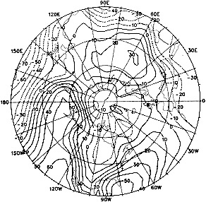
Figure 10
Correlations of the five-month mean (November to March) SOI with sea level pressures over the Northern Hemisphere for 1935 to 1991. The 1 percent significance level is 0.34.
persistence of the SOI is the factor contributing to the strong correlations when the SOI is leading. The lower values when the SOI is lagging are a reflection of the influence of the March-to-April time of year when the SOI tends to be weakest and preferentially changes sign (Trenberth, 1984).
However, this does not mean that there are not precursors in the tropics. On the contrary, it is well established that there is an evolution of the Southern Oscillation and the
TABLE 1 Correlations between the NP November-to-March Index, Indices of SST, and the SOI*
SST fields in the tropical Pacific as El Niño events develop (Trenberth, 1976; Rasmusson and Carpenter, 1982; Trenberth and Shea, 1987; Wright et al., 1988). Trenberth (1976), Trenberth and Shea (1987), and Wright et al. (1988) noted that pressures in the South Pacific (e.g., at Easter Island) respond about a season earlier than the SOI does, and Barnett (1985) suggested that changes can often be seen over the southeast Asian region before the SOI responds. Barnett et al. (1989) further suggested that this evolution might be linked to snow cover over Asia.
We have therefore examined in more detail the relationships between SSTs in the tropics and the NP index. Problems with data coverage are severe in the tropics prior to 1951. To help summarize the results, we have computed correlations between the area-averaged SST anomalies for the tropical Pacific Niño regions—Niño I and 2 (0 to 10°S, 90 to 80°W), Niño 3 (5°N to 5°S, 150 to 90°W), and Niño 4 (5°N to 5°S, 160°E to 150°W)—with NP at several leads and lags (see
Table 1). As larger areas are taken, the correlation coefficient increases in magnitude; for the Niño 3 and 4 regions combined, all correlations are larger, with maximum values of - 0.52 at a 3-month lead by the SSTs. This shows that the changes in SST throughout much of the tropical Pacific lead the NP index by about three months, although the cross-correlation is not sharply defined and values are only slightly smaller at zero lag. Nevertheless, these results emphasize the involvement of the tropical SST variations in the atmospheric and surface temperature variations over the North Pacific and North America.DISCUSSION AND CONCLUSIONS
The picture emerging from these empirical and modeling studies is not yet fully clear, but the evidence suggests the following hypothesis. In the tropics, coupled ocean-atmosphere interactions result in coupled modes, of which ENSO is the most prominent. This coupling results in large interannual variability in the Pacific sector, with preferred time scales of 2 to 7 years, but with small-amplitude decadal variations. All these fluctuations have manifestations in higher latitudes through teleconnections within the atmosphere. In the North Pacific, ENSO variability is found in the PNA pattern (and the NP index), but is best seen when averages can be taken over the entire winter half-year, because the noise level associated with natural weather variability is high on monthly time scales. The deepened Aleutian low in ENSO events results in a characteristic SST anomaly pattern that, on average, is enhanced through positive feedback effects from effects of the extratropical SST anomaly itself and from changes in momentum (and vorticity) fluxes associated with changes in high-frequency storm tracks (see Kushnir and Lau, 1992). The same influences are present on long time scales, but whereas surface fluxes and mixed-layer processes are dominant in changing SSTs on interannual time scales, changes in ocean currents also become a factor on decadal time scales and would reinforce the SST changes. Moreover, the long time scale involved in changing the currents and the Sverdrup circulation adds further persistence to the extratropical system that, along with heat storage in the top 500 m of the ocean, serves to emphasize decadal over interannual time scales.
Aspects of the above hypothesis have appeared in the extensive works of Namias, but here we have emphasized much more the links with the tropics. A major but as yet unanswered question is whether either the intensity or the frequency of ENSO events might change as a result of global warming. A longer observational record than that given in Figure 9 reveals that the frequency and intensity of ENSO events have changed in the past (Trenberth and Shea, 1987), with strong ENSO fluctuations from about 1880 to 1920. Aside from the major event from 1939 to 1942, stronger and more regular ENSO events did not resume until the 1950s. However, the low-passed curve in Figure 9 indicates that the recent imbalance between the
number of warm and cold events in the tropical Pacific is unprecedented.
Whether the unusual 1977-to-1988 imbalance can be ascribed in part to some identifiable contributor, or merely reflects natural variability, is a very difficult question to answer. The major change that occurred in March-to-April 1988, a transition from El Niño to a very strong La Niña (Figure 4), apparently ended the climate regime, although the underlying ocean currents and heat storage must be still perturbed and the pattern could reemerge. Indeed, the 19911992 ENSO event was noted for its exceptionally warm water along the west coast of both North and South America in early 1992.
ACKNOWLEDGMENTS
We wish to especially thank Dennis Shea for preparing some of the figures. This research is partially sponsored by the Tropical Oceans/Global Atmosphere Project Office under grant NA86AANRG0100.
Commentary on the Paper of Trenberth and Hurrell
YOCHANAN KUSHNIR
Lamont-Doherty Earth Observatory
Dr. Trenberth has demonstrated in this study how complex the middle-latitude system is. We have to deal with seasonality (there is a nice diagram in his paper that actually emphasizes the seasonality in this very-low-frequency phenomenon that he discussed). We also have to deal with the fact that middle latitudes filter the signal that comes out of the tropics, if it does indeed come out of the tropics as suggested here. Actually, the Pacific may be a more complex environment in which to study mid-latitude interactions than the Atlantic, where the effect of ENSO or of the tropics seems to be weaker.
One of the biggest issues in mid-latitude interaction is whether the ocean and the atmosphere are really coupled. It has been suggested that the ocean is being forced by the atmosphere and no feedback is involved. Local interactions like mixing and heat exchange, or maybe some non-local interactions due to the currents and transports, could be responsible for the fact that the pattern is long-lived. But why is it seen also in summer when the forcing from the atmosphere disappears, as the paper emphasizes?
If there is feedback in mid-latitude interactions, can we learn about it from GCMs? As it turns out, we are dealing with a very confusing set of results presented in several papers. They are confusing not only because of the use of super-anomalies versus regular anomalies, but also because different kinds of models and different kinds of methodologies have been used to run the models. We have seen perpetual experiments run, and we have seen experiments of a more transient nature where the seasonal cycle varies and where the SSTs vary continuously.
The coupling between the mid-latitude ocean and the atmosphere is one of the unresolved challenges today. It remains to be seen whether it is really a two-way interaction, and whether feedback in the middle latitudes is involved.
Discussion
BRYAN: This all reminds me of the Hoskins and Karoly ideas of about 12 years ago about the connection between the tropics and mid-latitudes.
TRENBERTH: Well, that may be one of the ways in which the whole system is tied together, but the statistical results indicate that it's probably more than just Southern Oscillation. The transients in the middle latitudes seem to be adding a considerable chaotic component to any teleconnections, and the forcing itself is different for every ENSO.
DICKSON: I worry a bit that your picture doesn't take into account the overlap of the North Atlantic and the Southern Oscillation signals that Rogers described in his 1984 paper. The biggest anomaly gradient of the lot sits on the boundary between them on the U.S. eastern seaboard, where there's such a strong land/ sea temperature contrast.
TRENBERTH: We can't treat those signals as linear and independent; I think the statistics indicate that there is a highly variable and sometimes strong connection between them. And I think there's a lot of feedback involved in the East Coast baroclinicity.
RASMUSSON: Yes, the correlation of all the oscillations in that area is fascinating. But the mean patterns in the North Pacific and
the tropics do seem to move in concert when the convection shifts, and I think that linkage is clear.
MARTINSON: Peter Weyl's 1967 climate scenario—90 percent of which has since been corroborated, I'd say—started with precipitation change in the Caribbean and the exchange of moisture between the Pacific and the Atlantic.
KARL: Kevin, I was interested in your comments on the character of the variance in the southeastern United States. Could you elaborate a little on those figures?
TRENBERTH: A figure in Leathers and Palecki (J. Climate, 1992), shows a step-like discontinuity in 1957. But I'm convinced that some of it isn't real, since it's only this one particular point that never returns to the pre-1957 level. There's some evidence of changes in analysis procedures or radiosondes.
CANE: It seemed to me that one difference between what you're doing and the older work was the emphasis on changes that persisted for most of a decade and the idea that the ocean's circulation would change and reinforce the SST pattern. How might the surface wind changes affect the ocean, and how consistent would that be with the SST pattern?
TRENBERTH: There's a nice figure in my 1991 paper showing the annual change in the wind stress. It's directly related to the change in the Aleutian system, and contributes substantially to a change in both the subtropical and the polar gyres in the North Pacific. It seems to me it wouldn't be hard to find out the actual spin-up time of a circulation change to a decent depth by using an ocean model; the typical number you hear is 10 to 30 years to really modify the basin-wide sverdrup transport.
Coupled Systems Reference List
Aceituno, P. 1992. El Niño, the Southern Oscillation and ENSO: Confusing names for a complex ocean-atmosphere interaction. Bull. Am. Meteorol. Soc. 73:483-485.
Alexander, M. 1992a. Mid-latitude atmosphere-ocean interaction during El Niño. Pt. I. The North Pacific Ocean. J. Climate 5:944-958.
Alexander, M. 1992b. Mid-latitude atmosphere-ocean interaction during El Niño. Pt. II. The Northern Hemisphere atmosphere. J. Climate 5:959-972.
Anderson, R.Y. 1989. Solar-cycle modulation of ENSO: A mechanism for Pacific and global climate change. Sixth Pacific Climate Workshop, Asilomar, Calif.
Bakun, A. 1990. Global climate change and intensification of coastal ocean upwelling. Science 247:198-201.
Barnett, T.P. 1985. Variations in near global sea level pressure. J. Atmos. Sci. 42:478-501.
Barnett, T.P. 1991. The interaction of multiple time scales in the tropical climate system. J. Climate 4:269-285.
Barnett, T.P., N. Graham, M.A. Cane, S.E. Zebiak, S. Dolan, J.J. O'Brien, and D. Legler. 1988. On the prediction of the El Niño of 1986-1987. Science 241:192-196.
Barnett, T.P., L.D.U. Schlese, E. Roeckner, and M. Latif. 1989. The effect of Eurasian snow cover on regional and global climate variations. J. Atmos. Sci. 46:661-685.
Battisti, D.S. 1988. Dynamics and thermodynamics of a warming event in a coupled tropical atmosphere-ocean model. J. Atmos. Sci. 45:2889-2919.
Battisti, D.S. 1995. Decade-to-century time-scale variability in the coupled atmosphere-ocean system: Modeling issues. In Natural Climate Variability on Decade-to-Century Time Scales. D.G. Martinson, K. Bryan, M. Ghil, M.M. Hall, T.R. Karl, E.S. Sarachik, S. Sorooshian, and L.D. Talley (eds.). National Academy Press, Washington, D.C.
Battisti, D.S., and A.C. Hirst. 1989. Interannual variability in the tropical atmosphere/ocean system: Influence of the basic state and ocean geometry. J. Atmos. Sci. 46:1687-1712.
Baumgartner, T. R., J. Michaelsen, L.G. Thompson, G.T. Shen, A. Soutar, and R.E. Casey. 1989. The recording of interannual climatic change by high-resolution natural systems: Tree rings, coral bands, glacial ice layers, and marine varves. In Aspects of Climate Variability in the Pacific and Western Americas. D.H. Peterson (ed.). Geophysical Monograph 55, American Geophysical Union, Washington, D.C., pp. 1-14.
Berlage, H.P. 1957. Fluctuations in the general atmospheric circulation of more than one year, their nature and prognostic value. Mededelingen en Verhandelingen, Kon. Ned. Met. Inst. 69, 152 pp.
Bjerknes, J. 1964. Atlantic air-sea interaction. Adv. Geophys. 10:1-82.
Bjerknes, J. 1969. Atmospheric teleconnections from the equatorial Pacific. Mon. Weather Rev. 97:163-172.
Blackmon, M.L., J.E. Geisler, and E.J. Pitcher. 1983. A general circulation model study of January climate anomaly patterns associated with interannual variation of equatorial Pacific sea surface temperatures. J. Atmos. Sci. 40:1410-1425.
Blumenthal, M.B. 1991. Predictability of a coupled ocean-atmosphere model. J. Climate 4:766-784.
Blumenthal, M.B., Y. Xue, and M.A. Cane. 1992. Predictability of an ocean/atmosphere model using adjoint model analysis. In Proceedings of the Workshop on Predictability, 13-15 November 1991. European Centre for Medium-Range Weather Forecasts.
Bond, G. W. Broecker, J. McManus, and R. Lotti. 1992. The North Atlantic's record of millennial-to-century scale climate changes and their link to Greenland ice core climate records. In NOAA Climate and Global Change Program Special Report No. 2, pp. 55-62.
Bottomley, M., C.K. Folland, J. Hsiung, R.E. Newell, and D.E. Parker. 1990. Global Ocean Surface Temperature Atlas
(GOSTA). Joint project of the Meteorological Office, Bracknell, U.K., and the Massachusetts Institute of Technology. HMSO, London, 20+ iv pp. and 313 plates.
Bradley, R.S. (ed.). 1991. Global Changes of the Past. UCAR/ Office for Interdisciplinary Earth Studies, Boulder, Colo., 514 PP.
Bradley, R.S., and P.D. Jones. 1992. Climate since A.D. 1500: Introduction. In Climate Since A.D. 1500. R.S. Bradley and P.D. Jones (eds.). Routledge, London, pp. 1-16.
Branstator, G., 1987. A striking example of the atmosphere's leading traveling mode. J. Atmos. Sci. 44:2310-2323.
Braudel, F. 1949. La Méditerranée et le monde Méditerranéen à l'époque de Philippe II. Colin, Paris, 1160 pp.
Bryan, F. 1986. High latitude salinity effects and inter-hemispheric thermohaline circulations. Nature 323:301-304.
Bryan, K. 1969. Climate and the ocean circulation. III: The ocean model. Mon. Weather Rev. 97:806-827.
Cane, M.A. 1991. Forecasting El Niño with a geophysical model. In ENSO Teleconnections Linking Worldwide Climate Anomalies: Scientific basis and societal impacts. M. Glantz, R. Katz, and M. Nicholls (eds.). Cambridge University Press, pp. 345-369.
Cane, M.A., S. Dolan, and S.E. Zebiak. 1986. Experimental forecasts of El Niño. Nature 321:827-832.
Cane, M.A., M. Münnich, and S.E. Zebiak. 1990. A study of self-excited oscillations of the tropical ocean-atmosphere system. Part I: Linear analysis. J. Atmos. Sci. 47:1853-1863.
Cane, M.A., S.E. Zebiak, and Y. Xue. 1995. Model studies of the long-term behavior of ENSO. In Natural Climate Variability on Decade-to-Century Time Scales. D.G. Martinson, K. Bryan, M. Ghil, M.M. Hall, T.R. Karl, E.S. Sarachik, S. Sorooshian, and L.D. Talley (eds.). National Academy Press, Washington, D.C.
Cayan, D.R. 1992. Latent and sensible heat flux anomalies over the northern oceans: The connection to monthly atmospheric circulation. J. Climate 5:354-369.
Cayan, D.R., and D.H. Peterson. 1989. The influence of North Pacific atmospheric circulation on streamflow in the West. Geophys. Monogr. 55:375-397.
Chao, Y., and S.G.H. Philander. 1993. On the structure of the southern oscillation. J. Climate 6:450-469.
Chatfield, C. 1989. The Analysis of Time Series: An Introduction. Chapman and Hall, London, 241 pp.
CLIMAP Project Members. 1981. Seasonal reconstruction of the Earth's surface at the last glacial maximum. Geol. Soc. Am. Map Chart Ser. MC-36.
Cole, J.E., R. Fairbanks, and G.T. Shen. 1995. Monitoring the tropical ocean-atmosphere using chemical records from long-lived corals. In Natural Climate Variability on Decade-to-Century Time Scales. D.G. Martinson, K. Bryan, M. Ghil, M.M. Hall, T.R. Karl, E.S. Sarachik, S. Sorooshian, and L.D. Talley (eds.). National Academy Press, Washington, DC.
Committee on Earth Sciences. 1989. Our Changing Planet: The FY 1990 Research Plan. The United States Global Change Research Program. OSTP FCCSET, Executive Office of the President.
Conover, W.J. 1980. Practical Non-Parametric Statistics. John Wiley and Sons, Inc., New York.
Crowley, T.J., and G.R. North. 1991. Paleoclimatology. Oxford Monographs on Geology and Geophysics, No. 16. Oxford Press, Oxford, 339 pp.
Cubash, U., K. Hasselmann, H. Hock, E. Maier-Reimer, U. Mikolajewicz, B.D. Santer, and R. Sausen. 1991. Time dependent greenhouse warming computations with a coupled ocean-atmosphere model. Report 67, Max Planck-Institut für Meteorologie, Hamburg, 18 pp.
D'Arrigo, R.D., G.C. Jacoby, and E.R, Cook. 1992. Decadal-scale variability of the North Atlantic atmosphere-ocean system as revealed by dendroclimatic evidence from surrounding land areas. In NOAA Climate and Global Change Program Special Report No. 2, pp. 45-53.
Davis, R. 1976. Predictability of sea surface temperature and sea level pressure anomalies over the North Pacific Ocean. J. Phys. Oceanogr. 6:249-266.
Davis, R. 1978. Predictability of sea-level pressure anomalies over the North Pacific Ocean. J. Phys. Oceanogr. 8:233-246.
Delworth, T., S. Manabe, and R.J. Stouffer. 1993. Interdecadal variations of the thermohaline circulation in a coupled ocean-atmosphere model. J. Climate 6:1993-2011.
Delworth, T.L., S. Manabe, and R.J. Stouffer. 1995. North Atlantic interdecadal variability in a coupled model. In Natural Climate Variability on Decade-to-Century Time Scales. D.G. Martinson, K. Bryan, M. Ghil, M.M. Hall, T.R. Karl, E.S. Sarachik, S. Sorooshian, and L.D. Talley (eds.). National Academy Press, Washington, D.C.
Deser, C., and M. Blackmon. 1991. Analysis of decadal climate variations over the Atlantic basin. In Proceedings of the Fifth Conference on Climate Variations. American Meteorological Society, Boston, pp. 470-471.
Deser, C., and M.L. Blackmon. 1995. Surface climate variations over the North Atlantic ocean during winter: 1900-1989. In Natural Climate Variability on Decade-to-Century Time Scales. D.G. Martinson, K. Bryan, M. Ghil, M.M. Hall, T.R. Karl, E.S. Sarachik, S. Sorooshian, and L.D. Talley (eds.). National Academy Press, Washington, D.C.
Deser, C., and J.M. Wallace. 1987. El Niño events and their relationship to the Southern Oscillation: 1925-86. J. Geophys. Res. 92:14189-14196.
Diaz, H.F., and V. Markgraf (eds.). 1992. El Niño: Historical and Paleoclimatic Aspects of the Southern Oscillation. Cambridge University Press, 440 pp.
Douglas, A.V., D.R. Cayan, and J. Namias. 1982. Large-scale changes in North Pacific and North American weather patterns in recent decades. Mon. Weather Rev. 112:1851-1862.
Ebbesmeyer, C.C., D.R. Cayan, D.R. McLain, F.H. Nichols, D.H. Peterson, and K.T. Redmond. 1991. 1976 step in the Pacific climate: Forty environmental changes between 1968-1975 and 1977-1984. In Proc. Seventh Annual Pacific Climate (PACLIM) Workshop, April 1990. J.L. Betancourt and V.L. Sharp (eds.). Interagency Ecological Studies Program Tech. Rept. 26, California Department of Water Research, Sacramento, Calif., pp. 129-141.
Elliot, W.P., and J.K. Angell. 1988. Evidence for changes in Southern Oscillation relationships during the last 100 years. J. Climate 1:729-737.
Enfield, D.B. 1992. Historical and prehistorical overview of El Niño: Historical and paleoclimatic aspects of the Southern Oscil-
lation. In El Niño: Historical and Paleoclimatic Aspects of the Southern Oscillation. H.F. Diaz and V. Markgraf (eds.). Cambridge University Press , Cambridge, U.K., pp. 95-117.
Enfield, D.B., and L. Cid. 1991. Low frequency changes in El Niño/Southern Oscillation. J. Climate 12:1137-1146.
Fairbanks, R.G., J. Cole, M. Moore, L. Wells, and G. Shen. 1992. The variance spectra of the Southern Oscillation under different climatological boundary conditions. In Paleo-ENSO Records International Symposium (Extended Abstracts). L. Ortlieb and J. Macharé (eds.). OSTROM-CONCYTEC, Lima, Peru, p. 101.
Folland, C., J. Owen, M.N. Ward, and A. Colman. 1991. Prediction of seasonal rainfall in the Sahel region using empirical and dynamical methods. J. Forecasting 10:21-56.
Frankignoul, C. 1985. Sea surface temperature anomalies, planetary waves, and air-sea feedbacks in middle latitudes. Rev. Geophys. 8:233-246.
Frankignoul, C., and K. Hasselmann. 1977. Stochastic climate models, Part II: Application to sea-surface temperature anomalies and thermocline variability. Tellus 29:289-305.
Glantz, M., R. Katz, and N. Nicholls. 1991. ENSO Teleconnections Linking Worldwide Climate Anomalies: Scientific basis and societal impacts. Cambridge University Press.
Gordon, C. 1989. Tropical-ocean-atmosphere interactions in a coupled model. Philos. Trans. Roy. Soc. London A329:207-223.
Gordon, A.L., S.E. Zebiak, and K. Bryan. 1992. Climate variability and the Atlantic Ocean. EOS 73:161-165.
Hamilton, K. 1987. Interannual environmental variation and North American fisheries. Bull. Am. Meteorol. Soc. 68:1541-1548.
Handler, P., and K. Andsager. 1990. Volcanic aerosols, El Niño, and the southern oscillation. J. Climatol. 10:413-424.
Hibler III, W.D., and K. Bryan. 1987. A diagnostic ice-ocean model. J. Phys. Oceanogr. 17:987-1015.
Hirst, A.C. 1988. Slow instabilities in tropical ocean basin-global atmosphere models. J. Atmos. Sci. 45:830-852.
Hocquenghem, A.M., and L. Ortlieb. 1992. Historical record of El Niño events in Peru (XVI-XVIII centuries): The Quinn et al. (1987) chronology revisited. In Paleo-ENSO Records International Symposium (Extended Abstracts). L. Ortlieb and J. Macharé (eds.). OSTROM-CONCYTEC, Lima, Peru, pp. 143-150.
Horel, J.D., and J.M. Wallace. 1981. Planetary-scale atmospheric phenomena associated with the Southern Oscillation. Mon. Weather Rev. 109:813-829.
IGBP. 1992. PAGES. J.A. Eddy (ed.). Global Change Report 19, International Geosphere-Biosphere Programme, Stockholm.
IPCC. 1990. Climate Change: The IPCC Scientific Assessment. J.T. Houghton, G.J. Jenkins, and J.J. Ephraums (eds.). Prepared for the Intergovernmental Panel on Climate Change by Working Group I. WMO/UNEP, Cambridge University Press, 365 pp.
IPCC. 1992. Climate Change 1992: The Supplementary Report to the IPCC Scientific Assessment. J.T. Houghton, B.A. Callander, and S.K. Varney (eds.). Prepared for the Intergovernmental Panel on Climate Change by Working Group I. WMO/UNEP, Cambridge University Press, 200 pp.
James, I.N., and P.M. James. 1989. Ultra-low frequency variability in a simple atmospheric model. Nature 342:53-55.
Jin, F.-F., and J.D. Neelin. 1992. Modes of interannual tropical ocean-atmosphere interaction—a unified view. Part I: Numerical results. J. Atmos. Sci. 50:3477-3503.
Jones, P.D. 1988. Hemispheric surface air temperature variations: Recent trends and an update to 1987. J. Climate 1:654-660.
Keigwin, L.D., and E.A. Boyle. 1992. Century and millennial-scale changes in North Atlantic surface and deep waters during the past 80,000 years. In NOAA Climate and Global Change Program Special Report No. 2, pp. 63-66.
Keppenne, C.L., and M. Ghil. 1992. Adaptive filtering and prediction of the Southern Oscillation Index. J. Geophys. Res. 97: 20449-20454.
Kushnir, Y. 1994. Interdecadal variations in North Atlantic sea surface temperature and associated atmospheric conditions. J. Climate 7: 141-157.
Kushnir, Y. and N.-C. Lau. 1992. The general circulation model response to a North Pacific SST anomaly: Dependence on time scale and pattern polarity. J. Climate 5:271-283.
Lanzante, J.R. 1984. A rotated eigenanalysis of the correlation between 700-mb heights and sea surface temperatures in the Pacific and Atlantic. Mon. Weather Rev. 112:2270-2280.
Latif, M., J. Biercamp, H. von Storch, and F.W. Zwiers. 1988. A ten-year climate simulation with a coupled ocean-atmosphere general circulation model. Report 21, Max Planck-Institut für Meteorologie, Hamburg.
Latif, M., A. Sterl, E. Maier-Reimer, and M.M. Junge. 1991. Climate variability in a coupled GCM. Part I: The tropical Pacific. J. Climate 6:5-21.
Latif, M., A. Sterl, E. Maier-Reimer, and M.M. Junge. 1993. Structure and predictability of the El Niño/Southern Oscillation phenomenon. J. Climate 6:700-708.
Lau, N.-C. 1988. Variability of the observed mid-latitude storm tracks in relation to low frequency changes in the circulation pattern. J. Atmos. Sci. 45:2718-2743.
Lau, N.-C., and M.J. Nath. 1990. A general circulation model study of the atmospheric response to extratropical SST anomalies observed in 1950-79. J. Climate 3:965-989.
Lazier, J. 1988. Temperature and salinity changes in the deep Labrador Sea, 1962-1086. Deep-Sea Res. 35:1247-1253.
Leathers, D.J., and M.A. Palecki. 1992. The Pacific North American teleconnection pattern and United States climate: 29 temporal characteristics and index specification. J. Climate 5:707-716.
Levitus, S. 1989a. Interpentadal variability of temperature and salinity at intermediate depths of the North Atlantic Ocean, 1970-1974 versus 1955-1959. J. Geophys. Res. 94:6091-6131.
Levitus, S. 1989b. Interpentadal variability of salinity in the upper 150 m of the North Atlantic Ocean. J. Geophys. Res. 94:9679-85.
Lorenz, E.N. 1963. Deterministic nonperiodic flow. J. Atmos. Sci. 20:130-141.
Lough, J.M., and H.C. Fritts. 1985. The Southern Oscillation and tree rings: 1600-1961. J. Clim. Appl. Meteorol. 24:952-966.
Ma, C.-C., C.R. Mechoso, A. Arakawa, and J.D. Farrara. 1994. Sensitivity of a coupled ocean-atmosphere model to physical parameterizations. J. Climate 7:1883-1896.
Madden, R.A., and P. Speth, 1989. The average behavior of large-scale westward traveling disturbances evident in the Northern Hemisphere geopotential heights. J. Atmos. Sci. 46:3225-3239.
Manabe, S. 1969a. Climate and the ocean circulation. I: The atmo-
spheric circulation and the hydrology of the earth's surface. Mon. Weather Rev. 97:739-774.
Manabe, S. 1969b. Climate and the ocean circulation. II: The atmospheric circulation and the effect of heat transfer by ocean currents. Mon. Weather Rev. 97:806-827.
Manabe, S., and R.J. Stouffer. 1988. Two stable equilibria of a coupled ocean-atmosphere model. J. Climate 1:841-866.
Manabe, S., R.J. Stouffer, M.J. Spelman, and K. Bryan. 1991. Transient response of a coupled ocean-atmosphere model to gradual changes of atmospheric CO2. Part I: Annual mean response. J. Climate 4:785-818.
Manabe, S., M.J. Spelman, and R.J. Stouffer. 1992. Transient response of a coupled ocean-atmosphere model to gradual changes of atmospheric CO2. Part II: Seasonal response. J. Climate 5:105-126.
Manak, D.K., and L.A. Mysak. 1987. Climatic atlas of arctic sea ice extent and anomalies, 1953-1984. Climate Research Group Report 87-8. McGill University, Montréal, 214 pp.
Mechoso, C.R., C.-C. Ma, J.D. Farrara, and J. Spahr. 1991. Simulations of interannual variability with a coupled atmosphere-ocean GCM. In Proceedings of Fifth Conference on Climate Variations. American Meteorological Society, Boston, pp. J1-J4.
Mechoso, C.R., A.W. Robertson, N. Barth, M.K. Davey, P. Delecluse, P.R. Gent, S. Ineson, B. Kirtman, M. Latif, H. Le Treut, T. Nagai, J.D. Neelin, S.G.H. Philander, J. Polcher, P.S. Schopf, T. Stockdale, M.J. Suarez, L. Terray, O. Thual, and J.J. Tribbia. 1995. The seasonal cycle over the tropical Pacific in coupled ocean-atmosphere general circulation models. Mon. Weather Rev. 123(9):2825-2838.
Michaelsen, J. 1989. Long-period fluctuations in El Niño amplitude and frequency reconstructed from tree rings. In Aspects of Climate Variability in the Pacific and the Western Americas. D.H. Peterson (ed.). Geophysical Monograph 55, American Geophysical Union, Washington, D.C., pp. 69-74.
Mikolajewicz, U., and E. Maier-Reimer. 1990. Internal secular variability in an ocean general circulation model. Climate Dyn. 4:145-156.
Münnich, M., M.A. Cane, and S.E. Zebiak. 1991. A study of self-excited oscillations of the tropical ocean-atmosphere system. Part 11: Nonlinear cases. J. Atmos. Sci. 48:1238-1248.
Mysak, L.A. 1986. El Niño interannual variability and fisheries in the northeast Pacific Ocean. Can. J. Fish. Aquatic Sci. 43:464-497.
Nagai, T., T. Tokioka, M. Endoh, and Y. Kitamura. 1991. El Niño/ Southern Oscillation simulated in an MRI atmosphere-ocean coupled general circulation model. J. Climate 5:1202-1233.
Namias, J. 1959. Recent seasonal interactions between North Pacific waters and the overlying atmospheric circulation. J. Geophys. Res. 64:631-646.
Namias, J. 1963. Large-scale air-sea interactions over the North Pacific from summer 1962 through the subsequent winter. J. Geophys. Res. 68:6171-6186.
Namias, J. 1969. Seasonal interactions between the North Pacific Ocean and the atmosphere during the 1960s. Mon. Weather Rev. 97:173-192.
Namias, J., X. Yuan, and D.R. Cayan. 1988. Persistence of North Pacific sea surface temperature and atmospheric flow patterns. J. Climate 1:682-703.
Neelin, J.D., M. Latif, M.A.F. Allaart, M.A. Cane, U. Cubasch, W.L. Gates, P.R. Gent, M. Ghil, N.C. Lau, C.R. Mechoso, G.A. Meehl, J.M. Oberhuber, S.G.H. Philander, P.S. Schopf, K.R. Sperber, A. Sterl, T. Tokioka, J. Tribbia. and S.E. Zebiak. 1992. Tropical air-sea interaction in general circulation models. Climate Dynamics 7:73-104.
Nicholls, N. 1988. Low Latitude Volcanic Eruptions and the El Niño Oscillation. J. Climatol. 8:91-95.
Nicholson, S.E. 1985. Sub-Saharan rainfall 1981-84. J. Clim. Appl. Meteorol. 24:1388-1391.
Nitta, T., and S. Yamada. 1989. Recent warming of tropical sea surface temperature and its relationship to the Northern Hemisphere circulation . J. Meteorol. Soc. Japan 67:375-383.
NOAA. 1990. The Atlantic Climate Change Program Science Plan. NOAA Climate and Global Change Program Special Report No. 2, UCAR, Boulder, Colorado, 29 pp.
NOAA. 1992. Proceedings from the Principal Investigators' Meeting of the ACCP. NOAA Climate and Global Change Program Special Report No. 7, UCAR, Boulder, Colorado.
Ortlieb, L., and J. Macharé (eds.). 1992. Paleo-ENSO Records International Symposium (Extended Abstracts). OSTROM-CONCYTEC, Lima, Peru, 333 pp.
Pan, Y.H., and A.H. Oort. 1990. Correlation analyses between sea surface temperature anomalies in the eastern equatorial Pacific and the world ocean. Climate Dynamics 4:191-205.
Parker, D.E., C.K. Folland, A.C. Bevan, M.N. Ward, M. Jackson, and K. Maskell. 1995. Marine surface data for analysis of climatic fluctuations on interannual-to-century time scales. In Natural Climate Variability on Decade-to-Century Time Scales. D.G. Martinson, K. Bryan, M. Ghil, M.M. Hall, T.R. Karl, E.S. Sarachik, S. Sorooshian, and L.D. Talley (eds.). National Academy Press, Washington, DC.
Parthsarathy, B., K. Rupa Kumar, and A.A. Munot. 1991. Evidence of secular variations in Indian monsoon rainfall-circulation relationships. J. Climate 4:927-938.
Philander, S.G.H., W.J. Hurlin, and A.D. Seigel. 1987. Simulation of the seasonal cycle of the tropical Pacific Ocean. J. Phys. Oceanogr. 17:1986-2002.
Philander, S.G.H., R.C. Pacanowski, N.C. Lau, and M.J. Nath. 1992. A simulation of the Southern Oscillation with a global atmospheric GCM coupled to a high-resolution, tropical Pacific Ocean GCM. J. Climate 5:308-329.
Phillips, N.A. 1956. The general circulation of the atmosphere: A numerical experiment. Quart. J. Roy. Meteorol. Soc. 82:123-164.
Pitcher, E.J., M.L. Blackmon, G.T. Bates, and S. Muñoz. 1988. The effects of North Pacific sea surface temperature anomalies on the January climate of a general circulation model. J. Atmos. Sci. 45:173-188.
Quinn, W.H., V.T. Neal, and S. Antunez de Mayolo. 1987. El Niño occurrences over the past four and a half centuries. J. Geophys. Res. 92:14449-14461.
Rabiner, L.R., M.R. Sambar, and C.E. Schmidt. 1975. Applications of nonlinear smoothing algorithm to speech processing. IEEE Trans. Acoust. Speech Signal Process. 23:552-557.
Rasmusson, E.M., and P.A. Arkin. 1993. A global view of large-scale precipitation variability. J. Climate 6:1495-1522.
Rasmusson, E.M., and T.H. Carpenter. 1982. Variations in tropical
sea surface temperature and surface wind fields associated with the Southern Oscillation/El Niño. Mon. Weather Rev. 110:354-384.
Rasmusson, E.M., X. Wang, and C.F. Ropelewski. 1990. The biennial component of ENSO variability. J. Mar. Syst. 1:70-96.
Rasmusson, E.M., X. Wang, and C.F. Ropelewski. 1995. Secular variability of the ENSO cycle. In Natural Climate Variability on Decade-to-Century Time Scales. D.G. Martinson, K. Bryan, M. Ghil, M.M. Hall, T.R. Karl, E.S. Sarachik, S. Sorooshian, and L.D. Talley (eds.). National Academy Press, Washington, D.C.
Rogers, J.C. 1984. The association between the North Atlantic oscillation and the southern oscillation in the northern hemisphere. Mon. Weather Rev. 112:1999-2015.
Rogers, J.C., and M.N. Raphael. 1992. Meridional eddy sensible heat fluxes in the extremes of the Pacific/North American teleconnection pattern. J. Climate 5:127-139.
Rogers, J.C., and R.V. Rohli. 1991. Florida citrus freezes and polar anticyclones in the Great Plains. J. Climate 4:1103-1113.
Ropelewski, C.F., and M.S. Halpert. 1987. Global and regional scale precipitation patterns associated with the El Niño/Southern Oscillation. Mon. Weather Rev. 115:1606-1626.
Ropelewski, C.F., and M.S. Halpert. 1989. Precipitation patterns associated with the high index phase of the Southern Oscillation. J. Climate 2:268-284.
Ropelewski, C.F., and P.D. Jones. 1987. An extension of the Tahiti-Darwin Southern Oscillation Index . Mon. Weather Rev. 115:2161-2165.
Ropelewski, C.F., M.S. Halpert, and X. Wang. 1992. Observed tropospheric biennial variability and its relationship to the Southern Oscillation. J. Climate 5:594-614.
Royer, T.C. 1989. Upper ocean temperature variability in the Northeast Pacific Ocean: Is it an indicator of global warming? J. Geophys. Res. 94:18175-18183.
Schopf, P.S., and M.J. Suarez. 1988. Vacillations in a coupled ocean-atmosphere model. J. Atmos. Sci. 45:549-566.
Semtner, A.J., Jr., and R.M. Chervin. 1988. A simulation of the global ocean circulation with resolved eddies. J. Geophys. Res. 93:15502-15522.
Shen, G.T., L.J. Linn, M.T. Price, J.T. Cole, R.G. Fairbanks, D.W. Lea, and T.A. McConnaughey. 1992. Paleochemistry of reef corals: Historical variability of the tropical Pacific. In Paleo-ENSO Records International Symposium (Extended Abstracts). L. Ortlieb and J. Macharé (eds.). OSTROM-CONCYTEC, Lima, Peru, pp. 287-294.
Shukla, J., and D.A. Paolino. 1983. The Southern Oscillation and long-range forecasting of the summer monsoon rainfall over India. Mon. Weather Rev. 111:1830-1837.
Stommel, H. 1961. Thermohaline convection with two stable regimes of flow. Tellus 13:224-230.
Tans, P., T. Conway, and T. Nakazawa. 1989. Latitudinal distribution of the sources and sinks of atmospheric carbon dioxide derived from surface observations and an atmospheric transport model. J. Geophys. Res. 94:5151-5172.
Thompson, L.G. 1992. Reconstructing the paleo-ENSO records from tropical and subtropical ice cores. In Paleo-ENSO Records International Symposium (Extended Abstracts). L. Ortlieb and J. Macharé (eds.). OSTROM-CONCYTEC, Lima, Peru, p. 311.
Thompson, P.D., E. Mosley-Thompson, and B.M. Brano. 1984. El Niño-Southern Oscillation events recorded in the Quelccaya Ice Cap, Peru. Science 226:50-53.
Ting, M. 1991. The stationary wave response to a mid-latitude SST anomaly in an idealized GCM. J. Atmos. Sci. 48:1249-1275.
Toggweiler, J.R., K. Dixon, and K. Bryan. 1989. Simulations of radiocarbon in a coarse-resolution world ocean model. II: Distributions of bomb-produced 14C. J. Geophys. Res. 94:8243-8264.
Trenberth, K.E. 1976. Spatial and temporal variations of the Southern Oscillation. Quart. J. Roy. Meteorol. Soc. 102:639-653.
Trenberth, K.E. 1984. Signal versus noise in the Southern Oscillation. Mon. Weather Rev. 112:326-332.
Trenberth, K.E. 1990. Recent observed interdecadal climate changes in the Northern Hemisphere. Bull. Am. Meteorol. Soc. 71:988-993.
Trenberth, K.E. 1991. Recent climate changes in the Northern Hemisphere. In Greenhouse-Gas-Induced Climate Change: A Critical Appraisal of Simulations and Observations. M. Schlesinger (ed.). Elsevier, Amsterdam/Oxford/New York, pp. 377-390.
Trenberth, K.E., and J.W. Hurrell. 1994. Decadal atmosphere-ocean variations in the Pacific. Climate Dynamics 9:303-319.
Trenberth, K.E., and J.W. Hurrell. 1995. Decadal climate variations in the Pacific. In Natural Climate Variability on Decade-to-Century Time Scales. D.G. Martinson, K. Bryan, M. Ghil, M.M. Hall, T.R. Karl, E.S. Sarachik, S. Sorooshian, and L.D. Talley (eds.). National Academy Press, Washington, D.C.
Trenberth, K.E., and D.A. Paolino. 1980. The Northern Hemisphere sea-level pressure data set: Trends, errors, and discontinuities. Mon. Weather Rev. 108:855-872.
Trenberth, K.E., and D.J. Shea. 1987. On the evolution of the Southern Oscillation. Mon. Weather Rev. 115:3078-3096.
Trenberth, K.E., J.R. Christy, and J.W. Hurrell. 1992. Monitoring global monthly mean surface temperatures. J. Climate 5:1405-1423.
Troup, A.J. 1965. The ''southern oscillation". Quart. J. Roy. Meteorol. Soc. 91:490-506.
van Loon, H. 1979. The association between latitudinal temperature gradient and eddy transport. Pt. I: Transport of sensible heat in winter. Mon. Weather Rev. 107:525-534.
Vautard, R., and M. Ghil. 1989. Singular spectrum analysis in nonlinear dynamics, with application to paleoclimatic time series. Physica 35D:395-424.
Vautard, R., P. Yiou, and M. Ghil. 1992. Singular spectrum analysis: A tool kit for short, noisy chaotic signals. Physica 58D:95-126.
Venrick, E.L., J.A. McGowan, D.A. Cayan, and T.L. Hayward. 1987. Climate and chlorophyll-a: Long-term trends in the central North Pacific Ocean. Science 238:70-72.
Vinnikov, K.Ya., P.Ya. Groisman, and K.M. Lugina. 1990. Empirical data on contemporary global climate changes (temperature and precipitation). J. Climate 3:662-677.
Walker, G.T. 1924. Correlation in seasonal variations of weather, IX: A further study of World Weather. Mem. Indian Meteorol. Dept. 24:275-332.
Walker, G.T., and E.W. Bliss. 1932. World Weather V. Mem. Roy. Meteorol. Soc. 4:53-84.
Wallace, J.M., and D.S. Gutzler. 1981. Teleconnections in the
geopotential height field during the northern hemisphere winter
. Mon. Weather Rev. 109:784-812.Wallace, J.M., and Q. Jiang. 1987. On the observed structure of the interannual variability of the atmosphere-ocean climate system. In Atmospheric and Oceanic Variability. H. Cattle (ed.). Roy. Meteorol. Soc., Bracknell, Berkshire, pp. 17-43.
Wallace, J.M., C. Smith, and Q. Jiang. 1990. Spatial patterns of atmosphere-ocean interaction in the northern winter. J. Climate 3:990-998.
Wallace, J.M., C. Smith, and C.S. Bretherton. 1992. Singular value decomposition of wintertime sea surface temperature and 500-mb height anomalies. J. Climate 5:561-576.
Walsh, J.E., W.D. Hibler III, and B. Ross. 1985. Numerical simulation of Northern Hemisphere sea ice variability, 1951-1980. J. Geophys. Res. 90:4847-4865.
Washington, W.M., and G.A. Meehl. 1989. Climate sensitivity due to increased CO2: Experiments with a coupled atmosphere and ocean general circulation model. Climate Dynamics 4:1-38.
Weaver, A.J., and E.S. Sarachik. 1991a. The role of mixed boundary conditions in numerical models of the ocean's climate. J. Phys. Oceanogr. 21:1470-1493.
Weaver, A.J., and E.S. Sarachik. 1991b. Evidence for decadal variability in an ocean general circulation model: An advective mechanism. Atmos.-Ocean 29:197-231.
Weaver, A.J., E.S. Sarachik, and J. Marotzke. 1991. Internal low frequency variability of the ocean's thermohaline circulation. Nature 353:836-838.
Winton, M., and E.S. Sarachik. 1993. Thermohaline oscillations induced by strong steady salinity forcing of ocean general circulation models. J. Phys. Oceanogr. 23:1389-1410.
Woodruff, S.D., R.J. Slutz, R.L. Jenne, and P.M. Steurer. 1987. A comprehensive ocean-atmosphere data set. Bull. Am. Meteorol. Soc. 68:1239-1250.
Wright, P.B., J.M. Wallace, T.P. Mitchell, and C. Deser. 1988. Correlation structure of the El Niño/Southern Oscillation phenomenon. J. Climate 1:609-625.
Zebiak, S.E. 1989. On the 30-60 day oscillation and the prediction of El Niño. J. Climate 2:1381-1387.
Zebiak, S.E., and M.A. Cane. 1985. A theory for El Niño and the Southern Oscillation. Science 228:1085-1087.
Zebiak, S.E., and M.A. Cane. 1987. A model El Niño-Southern Oscillation. Mon. Weather Rev. 115:2262-2278.
Zebiak, S.E., and M.A. Cane. 1991. Natural climate variability in a coupled model. In Greenhouse Gas-Induced Climatic Change: A critical appraisal of simulations and observations. M.E. Schlesinger (ed.). Elsevier, Amsterdam, pp. 457-470.
Zheng, D.-W., and D.-N. Dong. 1986. Realization of narrow band filtering of the polar motion data with multi-stage filter (translated). Acta Astron. Sin. 27:368-376.


