
Proxy Indicators of Climate: An Essay
SOROOSH SOROOSHIAN AND DOUGLAS G. MARTINSON
INTRODUCTION
Establishing a baseline of natural climate variability over decade-to-century time scales requires a perspective that can be obtained only from a better knowledge of past variability, particularly that which precedes the pre-industrial era. Information revealing these past climate conditions is contained in historical records and "proxy" indicators. The historical records of climate (other than systematic weather observations, which began in the late 1800s), while invaluable because of their scope and often uniquely relevant perspective, are usually limited to the last several hundred years (see Chapter 2). The proxy indicators represent any piece of evidence that can be used to infer climate. Typically, proxy evidence includes the characteristics and constituent compositions of annual layers in polar ice caps, trees, and corals; material stored in ocean and lake sediments (including biological, chemical, and mineral constituents); records of lake levels; and certain historical documents.
Such proxy indicators can provide a wealth of information on past atmospheric compositions, tropospheric aerosol loads, volcanic eruptions, air and sea temperatures, precipitation and drought patterns, ocean chemistry and productivity, sea-level changes, former ice-sheet extent and thickness, and variations in solar activity—among other things. These records are particularly appropriate for detecting three manifestations of climate variability:
-
Periodic or near-periodic variations (the latter are those that become evident only after examination of considerable data through which a clear statistical signal stubbornly emerges);
-
Large and pronounced climate signals, such as severe and sustained droughts, drastically altered precipitation patterns, anomalously warm or cold periods, or floods; and
-
Gradual trends, infrequent shifts, or other characteristics of natural variability that are difficult to recognize without the benefit of a long, continuous (or near-continuous) record.
Because the bulk of these proxy indicators are recorded naturally, their time span is potentially unlimited; their resolution and accuracy are limited only by the fidelity of the recorder itself. These "natural archives" are simply there for the taking—awaiting discovery, recovery, means of extraction, and interpretation. Consequently, proxy indicators represent a potential treasure trove of unique past climate information. The use of these data can present difficult problems of interpretation, particularly in light of the scanty spatial and temporal sampling, but can enhance our ability to reconstruct global changes. This chapter provides a state-of-the-art look at several aspects of this relatively new topic with respect to the climate of the last few millennia.
HISTORY OF PROXY INDICATORS
The use of proxy indicators in the study of modern climate draws on a broad range of disciplines and techniques. The potential of tree rings was recognized in the
early 1900s, when the 11 -year sunspot cycle was found to be recorded in the rings of trees in the southwestern United States. Major advances have been made since then, particularly within the last few decades. Many problems associated with interpretation of the rings (e.g., their causal relationship to climate) have been overcome, and the records have been extended from several hundred years to several thousand years or longer. Tree rings are now invaluable proxy indicators, because of their continuity and remarkable precision. In a similar vein, though more recently, the study of annual rings in massive corals is now yielding information regarding marine climates.
Many of the other proxy indicators, such as isotopes, fossil assemblages, and lake levels, had been used in the past to provide geological evidence in paleoclimate and paleoceanographic studies; they represent one of the standard tools in the geologist's arsenal. The relatively low resolution of the typical geological record had restricted their use chiefly to the study of long-time scale phenomena, such as glacial cycles. However, the desire to answer questions demanding higher-resolution data (for instance, whether the rapid climate excursions observed during the last deglaciation were anomalous, or were characteristic of a major climate transition) spurred improvements in the methods of recovery, analysis, and interpretation, which have yielded higher-resolution data. Improved collection techniques, such as long coring and better drilling methods, have made it possible to acquire the larger samples needed with the higher-resolution deposits; more natural data banks, such as ice caps and high deposition sediments, have been identified; and our understanding of both natural recorders and appropriate extraction techniques has increased, permitting higher precision with smaller samples.
All these developments are beginning to contribute to our knowledge of natural climate variability on decade-to-century time scales. Indeed, proxy indicators are now producing some of the most exciting and valuable records of variability to date. Furthermore, given the relatively embryonic state of the science, they have great potential for contributing to our understanding of the modern climate, particularly over longer time scales. New indicators are constantly being evaluated. For example, the use of biological ecosystems as proxy indicators of climate is demonstrated by McGowan (1995) and Reifsnyder (1995), both of which appear in this chapter. Numerous other proxy recorders—lake sediments, cave deposits, marshes—can now provide significant new insights. These are reviewed more thoroughly in Bradley and Jones (1992). In addition, the tremendous quantity of material in the historic records that is pertinent to climate is becoming increasingly useful, thanks to recent cataloguing that includes important metadata.
OCEANIC PROXY INSIGHTS
Numerous proxy indicators exist in the ocean, representing a wide spectrum of different oceanic and climate variables and spanning a wide range of time scales. Indicators residing in the sea-floor sediments may provide a nearly continuous record, often spanning tens of millions of years. These include pollen, faunal, and floral assemblages that have settled and accumulated, the isotopic compositions of skeletal material and tests from bottom-dwelling or floating organisms, and certain geological deposits and sediment types or compositions.
These ocean proxy records are accessible through sediment coring, drilling, and, in the case of certain bottom dwellers such as isolated corals, dredging. While the degrees of accuracy and resolution available vary, the information that can be extracted is staggering. For example (see the papers of Ruddiman and McIntyre, 1973; CLIMAP, 1981; and Imbrie et al., 1992 for more details), ocean proxy indicators have yielded regional information on the following characteristics: sea-surface and bottom temperature (from fossil assemblage composition), continental and landlocked ice volume and sea-level height (from oxygen isotope ratios), the partitioning of carbon between the land and oceans (from carbon isotope ratios), alkalinity of local water (from fossil preservation indices), deep-water circulation (from relative isotope compositions), surface productivity (from vertical isotope gradients), water-column stability (from radiolarian abundances), major front locations (from fossil, ice-rafted debris, and sediment-type distributions), deep-water temperature changes and surface salinity (from relative isotope compositions), vertical gradients of water-mass properties like temperature or salinity or of water-mass distributions (from analyses of sediments from different depths), deepwater velocity changes and source information (from sediment distributions near restricted passages), and predominant wind directions and intensities (from sediment compositions).
At typical sedimentation rates in the deep ocean basins (about 3 cm per 1000 years), sediment mixing serves as a low-pass filter, limiting the resolution of these proxy indicators to time scales of thousands of years. Regions in which the sediments accumulate faster offer the potential for resolving variations over significantly shorter time scales, but such areas often occur along continental margins where the interpretation of the sediment column is notoriously difficult, due to processes such as mass wasting. Consequently, until recently, these oceanic proxy indicators were used primarily to document and study climate variability on millennial or greater time scales. However, as Lehman (1995) explains in this chapter, areas with high deposition rates and relatively clean sediment records have now been located and sampled. These sample data are providing useful infor-
mation about natural variability and rapid climate change on time scales as short as decadal.
The paper in this chapter by Cole et al. (1995) describes the shorter, but often high-quality, records that can be found in the chemical composition of corals. Coral records spanning hundreds of years can be pieced together from a single region to provide information regarding sea surface temperature, upwelling, rainfall, and winds. Because corals often grow at rates three orders of magnitude greater than the rate of sediment accumulation in the deep sea, their temporal resolution is exceptionally good, providing high-fidelity records of natural variability on time scales as short as seasonal.
Finally, in addition to the oceanic proxy indicators preserved through time that are discussed above, some researchers have proposed that the spatial and temporal distributions of plankton and fish populations are intimately linked to ocean and climate conditions. The paper in this chapter by McGowan (1995) reviews the current state of our knowledge and discusses the problems in using such data as proxies for ocean/climate variabilities. McGowan's view of the relationships between climate and various proxies contrasts with the findings of Dickson (1995) that appear in Chapter 3. Their differences highlight the uncertainties surrounding this relatively new endeavor and the challenges associated with using highly complex biologic indicators.
ATMOSPHERIC PROXY INSIGHTS
Scientists have been examining a number of noninstrumental atmospheric proxy data sources in search of clues to past climate conditions. Each type of record contains information on one or more aspects of climate. Among these are historical documents (almost all aspects of climate), tree rings (temperature, precipitation, pressure patterns, drought, and runoff), ice cores (temperature, precipitation, atmospheric aerosols, atmospheric composition, and more), lake levels (runoff and drought patterns), and varved sediments (temperature, precipitation, and solar radiation). With the exception of the historical documents, perhaps, the climate information in these proxy indicators must be isolated from the nonclimate portion of the signal and any accompanying noise.
Of the various sources of atmospheric proxy indicators, the greatest attention has so far been given to the use of historical documents, tree rings, and ice cores. (Of these, tree rings have been subjected to the most rigorous testing as sources of information on past climate.) A number of papers in this volume make reference to non-instrumental records, primarily tree rings (Jones and Briffa, 1995; Cook et al., 1995b, and Reifsnyder, 1995, all in this chapter; and Diaz and Bradley, 1995, in Chapter 2.) The uses of ice cores (Grootes, 1995, in this chapter), which reflect past temperatures, and of lake levels (Street-Perrott, 1995, in this chapter), which reflect overall net moisture supply to the landscape, are presented as well.
The paper in this chapter by Jones and Briffa (1995) sets out to show the potential value of proxy records by looking at dendroclimate reconstructions of summer temperatures of four regions: northern Fennoscandia, the northern Urals, Tasmania, and northern Patagonia. In none of the thousand-year reconstructions did the twentieth century stand out as the warmest century, although it was among the warmest. Jones and Briffa also provide a useful discussion of the potential limitations of single-site dendroclimate reconstruction, and of the difficulties and uncertainties associated with comparison of multi-site records. Similar limitations can be expected to apply to other site-specific proxy indicators, so they represent a general caution about the interpretation of climate proxy records.
Despite the limitations, these long tree-ring records clearly document large and pronounced climate signals, such as the century-long cold period beginning in 1550. Tree-ring evidence is of critical importance in establishing the magnitude and duration of natural climate anomalies, since the instrumental records are too short to do so and also may reflect anthropogenic contamination. In addition, the tree-ring data can provide key information for the interpretation of gradual trends in climate. For example, they show that the period from 1880 to 1910 was anomalously warm throughout much of the Northern Hemisphere. Thus, the apparent magnitude of the present warming trend will depend on when the selected period begins.
The contribution to this chapter of Cook et al. (1995b) examines the power spectrum of a 2290-year reconstruction of warm-season Tasmanian temperatures to detect signs of periodic decadal-scale fluctuations. The paper suggests that the decadal-scale temperature anomalies over Tasmania during the twentieth century, both warm and cold, have been driven in part by long-term climate oscillations. It neither supports nor eliminates greenhouse warming as a possible contributor to the recent temperature increase in Tasmania. However, their study also investigates mechanisms of climate change that are testable (e.g., internal forcing related to deep-water formation, or external forcing by long-term solar variability) and provides specific explanations of synoptic-scale variability (e.g., the expansion and contraction of the circumpolar vortex).
Grootes (1995, in this chapter) discusses the potential role of ice-core records in reconstructing decade-to-century-scale climate variations. He seems confident that the new ice-core records being obtained from the summit of the Greenland ice sheet provide an accurate and remarkably detailed history of changes in climate over the North Atlantic basin as far back as 200,000 years ago. Indeed, there is little doubt as to the potential utility of the high-resolution, fast-response climate records from ice cores. At present, however, they can be obtained only from high-latitude or
high-altitude locations, and few of the ice-core reconstructions of temperature have been explicitly calibrated against instrumental time series. The differences between ice-core records from various sites also make it clear that there is a pressing need to identify and differentiate the relative influences of local mesoscale and hemispheric atmospheric factors.
In her paper in this chapter, Street-Perrott (1995) discusses how fluctuations in the water level and surface area of relatively undisturbed lakes (i.e, there has been no human-induced change in the water budget) can provide a measure of climate variability on time scales of months to millions of years. The paper provides examples of the response of tropical lakes to variations in ocean-atmosphere interactions over the Pacific (Lake Pátzcuaro), the Indian Ocean (Lake Victoria), and the Atlantic (Lake Chad, Lake Malawi), and points to paleolimnological evidence for century-scale droughts in southern Africa and the tropical Americas.
Finally, Reifsnyder (1995, in this chapter) analyzes observational and paleoclimate records of temperature in an attempt to determine the realism of models' predicted global-warming rates. Some models predict a rate of warming that is 10 to 40 times faster than the natural warming that followed the last ice age. On the basis of his analysis, however, Reifsnyder argues that the climate change between now and the end of the next century, for a "business as usual" scenario, should take place at no more than twice the maximum rate estimated for changes since the last ice age. He further argues that, because models are known to overpredict by a factor of two the rate of change over the past century in response to the CO2 increase, the rate of global warming over the next century is in fact unlikely to be higher than any estimated post-ice-age maximum rate— a position which certainly could generate a lot of debate, given the other forcings likely to be operating.
Soil and varved sediments, and historical documents, are two sources of atmospheric proxy data that are not covered in this volume. Sedimentary and soil cores can reveal significant paleoclimate information. For example, in a recently published paper in Science, Weiss et al. (1993) attributed the demise of the Akkadian culture (fl. 3000 B.C.) of southern Mesopotamia (present-day northeast Syria) in 2200 B.C. to an abrupt change in climate. The combined archaeological and soil-stratigraphic data for the area point to a shift in climate toward the arid, and a dry period persisting for about 300 years.
A variety of historical sources, such as ancient inscriptions, personal diaries and correspondence, scientific and quasi-scientific writings, government records, and public and private chronicles and annals record climate events that were seen as having some significance at the time. The information may include observations of weather phenomena, such as the occurrence of extreme rain- and snowfalls, droughts, floods, or lake and river freeze-ups and breakups. Historical records, unfortunately, fail to give a complete picture of former climate conditions. They are often discontinuous observations, biased towards extreme events. The important long-term trends tend to go unremarked. A good source of discussions of documentary records of past climate is the recently published book by Bradley and Jones (1992).
CURRENT LIMITATIONS
While proxy indicators are extremely important, even crucial, to climate reconstruction, their limitations should be kept in mind. The most significant are:
-
It is not always clear whether the signal they record reflects only local conditions, or is representative of regional or global conditions.
-
Their accuracy is often unknown or untested.
-
They often reflect more than one variable, making interpretation difficult.
-
The absolute, and even the relative, timing of the record is often not certain.
Bradley and Eddy (1989) stressed the importance of the last of these limitations, and noted that without accurate dating it is impossible to determine whether certain events occurred synchronously or not. In the Vostok ice core of central East Antarctica, for example, variations in air temperature (Jouzel et al., 1987) and atmospheric CO2 concentration (Barnola et al., 1987) have been reconstructed for the last 160,000 years. Within the dating uncertainties, these records show striking correspondence between high CO2 concentrations and warm temperatures. However, whether the increases in CO2 concentration precede or follow the temperature increases cannot be assessed accurately from these records.
Accurate dating is also a problem in attempting to overcome the first limitation listed above. That is, in order to reconstruct a global picture of climate at a given time, it is necessary to reconstruct climate variables from a number of different locations for that time. The accurate dating needed to establish the relationships of the various records is not always available. This problem plagues most of the ocean records, because distinct annual varves are rarely present. Dating is mostly accomplished through other techniques, again of limited accuracy, which constrains the degree to which comparisons can be made. Sowers et al. (1993) attempted to relate the variations in the Vostok ice record to those in the ocean by correlating supposedly globally synchronous changes in oxygen isotope concentrations. This technique has met with some success, but the range of error precludes comparisons over time scales less than millennial.
Other limitations arise because recording is often discontinuous. For instance, the recording mechanism may be disturbed during or after the recording, or the recovery may
be incomplete. This introduces gaps or perturbations that disguise or break the general patterns. An excellent example of the type of inconsistencies that may occur from the different recording properties of different climate proxies is provided by Grootes's (1995) paper in this chapter. However, the promising news in this area is that more researchers are reporting long-term reconstructions from different proxy sources and different geographic locations. The latest is the study by Lara and Villalba (1993) of a 3620-year reconstructed temperature record from alerce trees (Fitzroya cupressoides) from southern Chile. Their work, which has shown the alerce tree as being the second longest-living tree after the bristlecone pine, expands the availability of long-term climate records for the Southern Hemisphere.
In Chapter 2 Diaz and Bradley (1995) provide a useful discussion of a number of potential sources of uncertainties and biases associated with climate variable reconstruction, even for the relatively well-understood tree rings. They warn that changes over time in the composition of the tree-ring network used for reconstruction are likely to affect the high-frequency variance and, to some extent, the low-frequency variance as well. Considerable effort has been made to reduce the uncertainties associated with the long-term reconstruction of climate variables from the composition of tree-ring samples. For instance, an index value (temperature, for instance) for a given site is obtained from samples of trees that may vary considerably in age or even be dead. Attention must therefore be given during the reconstruction analysis to getting the chronology right for every tree; removing the biological growth trend; identifying the nature of the climate signal and its strength; replication; and the way in which the analysis method deals with changes in site conditions over the recorded interval. As a result of this careful scrutiny, tree-ring records exhibit exceptionally high fidelity, with comparatively minor interpretational problems. Similar sets of considerations must be addressed for other proxy indicators, no doubt including some not yet identified.
THE FUTURE OF PROXY INDICATORS
It is clear that accurate dating is required to assess the rate at which past climate changes have occurred and to reconstruct globally synchronous records of climate, particularly for changes on time scales of less than a century. The duration of high-frequency, short-term events may be less than the normal error associated with most methods used in dating the proxy records available. The issue of dating thus merits continued attention. Similarly, a sustained effort must be made to identify problems and uncertainties in reconstructions based on proxy indicators and to assess the associated errors; this should come naturally with increased experience in these relatively novel techniques. Last. combining records that have been drawn from different areas and that use different types of indicators into a consistent picture will be crucial for the study and reconstruction of global climate variations.
Finally, as with climate modeling, the reconstruction of past climates requires the employment of a full range of different proxy indicators. These must be developed more fully so that they can be used to intercalibrate the reconstructed climates and cross-check the reconstructions; to provide multiple images of climate through different climate indicators; and to reduce the influence of noise through averaging. In this early stage, we are seeing only the tip of the iceberg; the results of the use of proxy indicators only hint at the climate insights yet to be won by means of these invaluable resources.
Monitoring the Tropical Ocean and Atmosphere Using Chemical Records from Long-Lived Corals
JULIA E. COLE1, RICHARD G. FAIRBANKS2, AND GLEN T. SHEN3
ABSTRACT
The tropical ocean and atmosphere constitute an active component of the global climate system on interannual-to-century time scales, yet instrumental climate records from this extensive region are scarce, short, and unevenly distributed. Geochemical records from corals offer a promising means of extending the record of tropical climate variability. Corals grow rapidly (more than 1 cm/yr), may live for several centuries, are datable by several independent means, and incorporate the signatures of key atmospheric and oceanic processes in their skeletal chemistry. Efforts to extend coral records beyond the instrumental period and to recover Holocene and deglacial-age samples are under way throughout the tropics. Coral-based reconstructions of the El Niño/Southern Oscillation (ENSO) phenomenon demonstrate how this approach can contribute to understanding past variability in tropical climate dynamics.
The abundance of atolls and coral reefs in the tropical Pacific enables coral studies to target specific features of ENSO, including variability in sea surface temperatures, upwelling, rainfall, and winds. Short records from three sites spanning the Pacific show coherent variations in these parameters associated with warm and cool ENSO extremes. In the Galapagos Islands, a tracer intercomparison study from a single coral head demonstrates high correlations with measured ENSO-related variability between 1936 and 1982, especially for the interannual periods characteristic of ENSO. Farther west, a coral record from Tarawa Atoll closely monitors central-western Pacific rainfall over the past century. Evolutionary spectral analysis of this record suggests a mode of variation between about 1930 and 1950 that differs from preceding or subsequent periods. Over the span of this coral record, variance at the annual cycle has been weakest during the past few decades. Between 1930 and 1950, however, the annual cycle reaches a magnitude comparable to that of the interannual variations, and a strong 3-year component virtually disappears. This shift occurs concurrently with an observed weakening of the Southern Oscillation and its teleconnections.
INTRODUCTION
The tropical ocean and atmosphere constitute an active component of the global climate system, especially on sub-millennial time scales. Understanding the climatic processes that act on these time scales across this extensive region requires that we characterize their past variability. Yet instrumental records from the sparsely inhabited tropical oceans are scarce and short. Those records that extend beyond the past few decades often owe their locations to opportunistic, rather than climatic, rationales. Chemical records from the skeletons of long-lived corals provide one of the few high-quality means for extending the length of the climatic record in the tropical oceans beyond the brief period of instrumental coverage. Coral records offer an unusual opportunity to monitor the history of key tropical climate systems, especially since sites and tracers can be chosen explicitly for their climatic relevance. The development of proxy climate records from coral archives promises to offer important insights into the natural patterns and causes of tropical climate change, and into the sensitivity of low-latitude oceans to shifts in the global boundary conditions of climate. In the tropical Pacific, we have found that short records of isotopic and trace-metal variability in coral skeletons closely track specific ocean-atmosphere processes over the past few decades. An examination of multiple tracers within a single coral specimen demonstrates the varied utility of isotopic and trace-metal variations in tracking interannual sea surface temperature (SST) and upwelling changes. A 96-year record from the equatorial region west of the date line provides an index of ENSO variability comparable in quality to climatological records, and suggests that the spectrum of climate variability in this region has varied over the course of the present century.
Tropical climate variability may take many forms; describing variations in tropical ocean-atmosphere systems thus requires a multivariate approach capable of resolving specific processes. SST changes dramatically over annual-to-interannual periods in regions of upwelling such as the eastern Pacific, eastern Atlantic, and northern Indian oceans, while SST in the western basins of tropical oceans tends to vary much less. Changes in upwelling have important consequences for surface ocean chemistry as well as for temperature. Surface levels of nutrients and other dissolved species enriched in deep water also vary in accordance with the upwelling of deep water to the surface. Advective changes have site-dependent effects on both chemical and thermal distributions. Patterns of rainfall and wind may shift in response to changed SST distribution; they in turn alter the thickness and salinity of the ocean's surface mixed layer, which affect the degree of ocean-atmosphere interaction (Godfrey and Lindstrom, 1989; Lukas and Lindstrom, 1991). Significant changes in SST, surface upwelling, currents, rainfall, and winds may result from interactions within the tropical ocean-atmosphere system. Alternatively, such changes may be forced by continental systems, such as the Asian monsoon. Many chemical tracers in coral skeletons possess distinct sensitivities to specific environmental variables such as SST, rainfall, winds, and upwelling; as with instrumental data, many coral records monitor specific oceanic or atmospheric processes. Reconstructing the behavior of large-scale, multivariate climate systems such as the El Niño/Southern Oscillation (ENSO) will require the integration of many such coral indices over extensive regions (Figure 1).
CORAL RECORDS
Individual coral heads may live for several centuries, offering the potential for climate reconstructions from remote sites that predate even the longest instrumental records. Because they grow at rates of 1 to 2 cm/yr and can be sampled at intervals less than I mm, records at sub-monthly resolution are obtainable. Interpretation of such long, high-resolution records demands precise chronologies.
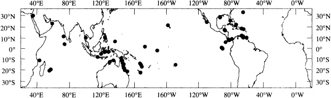
Figure 1
Map showing the distribution of sites where living coral heads have been cored for paleoclimatic analysis (after Dunbar and Cole, 1993). Sites with long records are mentioned in the text.
Corals can be dated over a wide range of time scales (from seasons to periods greater than 100,000 years) by a variety of independent means, including density and fluorescent banding, 230Th/234U ratio, 14C content, stable-isotope fluctuations, and amino acid racemization (Dodge et al., 1974; Isdale, 1984; Edwards et al., 1988; Fairbanks, 1989, 1990; Bard et al., 1990; Cole and Fairbanks, 1990; Goodfriend et al., 1993). Recent work on monthly and even daily coral banding offers the promise for increasingly refined chronological determinations (Barnes and Lough, 1989; Risk and Pearce, 1992).
Corals precipitate a skeleton of aragonite (CaCO3) that can incorporate several independent chemical tracers used to monitor variability in oceanic and atmospheric processes. The most consistently useful of these are the isotopic ratios of carbon and of oxygen in particular, and the concentration of certain lattice-bound trace metals that appear to substitute for skeletal calcium (expressed as Cd/Ca, Ba/Ca, Mn/Ca, and Sr/Ca ratios). In this section, we present an overview of the many tracers now in use for coral-based paleoclimatic reconstruction. Subsequent sections discuss examples of both short records from a variety of sites and longer records that yield insight into the recent history of tropical climate variability.
Isotopic Indicators
The stable isotopic content of coral aragonite is expressed in parts per thousand (![]() ) as d180 and d13C, where the d notation is defined in terms of the isotopic ratios R (either 13C/12C or 18O/16O) in the sample relative to a standard:
) as d180 and d13C, where the d notation is defined in terms of the isotopic ratios R (either 13C/12C or 18O/16O) in the sample relative to a standard:
d = [(Rsample - Rstandard)/Rstandard] × 1000
For the oxygen and carbon isotopic content of coralline aragonite, the conventional reference standard is the Pee Dee Belemnite, or PDB.
Coral skeletal d18O reflects a combination of local SST and the d18 O of ambient seawater. The d18O of biogenic calcium carbonate precipitated in equilibrium with seawater decreases by about 0.22 ![]() for every 1°C rise in water temperature (Epstein et al., 1953). In corals, this effect is biologically mediated such that the d18O of the coral skeleton is offset below seawater d18O. This offset is constant within a coral genus (Weber and Woodhead, 1972) for the rapidly growing central axis of the skeleton (Land et al., 1975; McConnaughey, 1989). Coral d18O records taken along the axis of maximum growth thus track ambient temperatures at subseasonal resolution (Fairbanks and Dodge, 1979; Dunbar and Wellington, 1981; Pätzold, 1984; McConnaughey, 1989). Coral skeletal d18O also records any variations in the d18O of the seawater (Epstein et al., 1953; Fairbanks and Matthews, 1979; Swart and Coleman, 1980). Such variations are small in most regions of the tropical ocean, but in some locations changes in evaporation, precipitation, or runoff may cause pronounced d18O variability (Dunbar and Wellington, 1981; Cole and Fairbanks, 1990). In regions with fairly constant or well-known temperature histories, coral d18O provides a record of past variations in the hydrologic balance (Cole and Fairbanks, 1990). In many cases, coral skeletal d18O reflects a combination of thermal and hydrologic factors.
for every 1°C rise in water temperature (Epstein et al., 1953). In corals, this effect is biologically mediated such that the d18O of the coral skeleton is offset below seawater d18O. This offset is constant within a coral genus (Weber and Woodhead, 1972) for the rapidly growing central axis of the skeleton (Land et al., 1975; McConnaughey, 1989). Coral d18O records taken along the axis of maximum growth thus track ambient temperatures at subseasonal resolution (Fairbanks and Dodge, 1979; Dunbar and Wellington, 1981; Pätzold, 1984; McConnaughey, 1989). Coral skeletal d18O also records any variations in the d18O of the seawater (Epstein et al., 1953; Fairbanks and Matthews, 1979; Swart and Coleman, 1980). Such variations are small in most regions of the tropical ocean, but in some locations changes in evaporation, precipitation, or runoff may cause pronounced d18O variability (Dunbar and Wellington, 1981; Cole and Fairbanks, 1990). In regions with fairly constant or well-known temperature histories, coral d18O provides a record of past variations in the hydrologic balance (Cole and Fairbanks, 1990). In many cases, coral skeletal d18O reflects a combination of thermal and hydrologic factors.
The interannual d13C signal in coral skeletons is often difficult to decipher in environmental terms, because of complicated interactions with biological processes that involve strong isotopic fractionation. Environment-related controls on skeletal d13C include (1) the isotopic composition of the ambient seawater (Nozaki et al., 1978), (2) coral geometry and growth rate (e.g., apex versus side of coral head) (Land et al., 1975; McConnaughey, 1989), and (3) photosynthesis of endosymbiotic dinoflagellates (Weber, 1974; Goreau, 1977; Fairbanks and Dodge, 1979; Swart, 1983; McConnaughey, 1989). This last parameter depends upon ambient light levels, as regulated by water depth and insolation. Coral skeletal d13C correlates positively with insolation in many contexts, from depth-dependent variation (Weber and Woodhead, 1970; Fairbanks and Dodge, 1979; McConnaughey, 1989) to annual cycles that reflect rainy (i.e., cloudy) seasons (Fairbanks and Dodge, 1979; Pätzold, 1984; McConnaughey, 1989; Cole and Fairbanks, 1990). However, shallow corals may experience reduced photosynthesis during brighter periods, while deeper corals may respond to increased light by increasing photosynthesis (Erez, 1978; McConnaughey, 1989). These responses can produce opposite skeletal d13C signatures in deep and shallow corals (McConnaughey, 1989). Environmental reconstruction from coral d13C records requires more information about growth conditions and physiological responses than is usually available in a paleoceanographic context.
Trace Metals
Specific environmental processes, including upwelling, advection, aeolian transport, and runoff, influence the surface-water concentrations of certain trace elements (Boyle, 1988; Martin et al., 1976; Shen and Boyle, 1988; Lea et al., 1989; Shen and Sanford, 1990; Shen et al., 1991, 1992b). Several such metals appear to substitute readily for Ca in the aragonite lattice of coral skeletons. Estimated distribution coefficients between corals and seawater allow the reconstruction of ambient seawater metal concentrations from metal concentrations in the coral skeleton. Trace metal records from corals thus yield a history of the processes that control the local distribution of trace metals.
The most useful metals for coral reconstructions of ENSO variability include Cd, Ba, Mn, and Sr. Many authors (Shen and Boyle, 1988; Lea et al., 1989; Linn et al., 1990; Shen and Sanford, 1990; Shen et al., 1987, 1991; Beck et al., 1992; de Villiers et al., 1993) describe these applications
in greater detail, including specific techniques for sample cleaning and analysis. Studies of growth rate and species influences show very limited evidence of biological mediation of metal incorporation (de Villiers et al., 1993; G.T. Shen, unpublished results). However, SST may play a role in the incorporation of Ba (Lea et al., 1989), and the dependence of Sr incorporation on ambient SST (Smith et al., 1979) makes possible precise reconstruction of SST from coral Sr records (Beck et al., 1992).
Cadmium
The modern distribution of cadmium follows that of marine nutrients. Low levels in surface waters reflect biological removal, while higher levels at depth result from the regeneration of organic matter (Boyle et al., 1976; Martin et al., 1976). In coral records, the skeletal Cd content usually depends on the balance between Cd-rich upwelled deep water and Cd-poor oligotrophic surface waters. In Galapagos corals, Cd/Ca ratios directly reflect upwelling variations associated with both seasonal cycles (Linn et al., 1990; Shen and Sanford, 1990) and interannual ENSO variability (Shen et al., 1987, 1992a).
Barium
This trace metal exhibits nutrient-like behavior akin to cadmium's (Chan et al., 1977). Higher concentrations in both seawater and corals render coral Ba records less susceptible to contamination. Seasonal-resolution records of Ba/Ca from Galapagos corals reflect regional upwelling variability (Lea et al., 1989). Relative to Cd, Ba may exhibit greater sensitivity to periods of weak upwelling, possibly because the biological uptake of Cd occurs at rates comparable to the slow rate of supply during these times. Ba is also enriched in continental runoff waters, and Ba/Ca records from corals near continental margins may reflect this input (Shen and Sanford, 1990). However, a slight temperature effect may occur upon incorporation of Ba into the coral skeleton, which would complicate paleoclimatic reconstruction from coral Ba/Ca records (Lea et al., 1989).
Manganese
Unlike Cd and Ba, Mn reaches high concentrations in surface waters. A mid-depth maximum coincides with the local O2-minimum zone, where particulate Mn oxides are reduced and solubilized; concentrations then diminish with increasing depth. Aeolian and fluvial input provide important Mn sources, as do reducing environments where particulate Mn is degraded, such as the O2-minimum zone, shelf sediments, and lagoons. The interpretation of coral Mn/Ca records is thus usually site-specific, reflecting transport and mixing of water masses with varying Mn levels. In the Galapagos, for example, seawater Mn levels reflect a combination of aerosol deposition on the surface waters and long-range advection of Mn-enriched surface water from the continental shelf (Shen et al., 1991). In localized reef settings, dissolved Mn in the water column can be augmented by local sediment fluxes, producing very high skeletal concentrations of Mn in corals from the Gulf of Panama and some Caribbean islands (Shen et al., 1991). Diagenetic Mn fluxes from lagoonal sediments offer useful indicators of climate variability at certain Pacific atoll sites far removed from continental sources of Mn (Shen et al., 1992b).
Strontium
Work by Smith et al. (1979) demonstrated that the Sr/ Ca ratio of coral skeletons may provide a monitor of past temperature changes. However, the measurement technique used in that study was not sufficiently precise to offer detailed SST reconstructions at a useful resolution for the tropics. The recent application of thermal ionization mass spectrometry (TIMS) to these measurements has greatly improved the precision of Sr/Ca determinations (Beck et al., 1992); recent results indicate that monthly SST can be reconstructed with an apparent accuracy of better than 0.5°C (Beck et al., 1992; de Villiers et al., 1993). SST reconstructions based on skeletal Sr determinations are less susceptible to artifacts associated with hydrologic changes than d18O-based reconstructions. The paired application of d18O and Sr/Ca data may thus allow the separation of SST changes from seawater d18O variability.
Paleoceanographic Applications
Many studies have documented the paleoclimatic utility of isotopic and trace-metal measurements by developing short (2-20 yr) data sets that correlate with nearby instrumental records (e.g., Fairbanks and Dodge, 1979; Pätzold, 1984; Shen et al., 1987, 1992b; Carriquiry et al., 1988; Lea et al., 1989; Cole and Fairbanks, 1990; Winter et al., 1991; Cole et al., 1992; Beck et al., 1992). With the growing interest in long records of natural climate variability, many groups are applying these techniques to the development of proxy records that extend beyond the period of local instrumental coverage. Efforts to develop long, high-resolution reconstructions of climate are in progress using coral records from sites throughout the low-latitude oceans. Several studies have focused explicitly on reconstructing interannual-to-decadal variability in the ENSO system; we detail current results from the equatorial Pacific in the following section. Other sites from which coral records extending beyond the present century have been developed include Florida Bay (Kramer et al., 1991), Cebu Island, Philippines (Pätzold and Wefer, 1986), Espiritu Santo Island (Quinn et al., 1992), the southern Great Barrier Reef (Druffel and
Griffin, 1992), Bermuda (Pätzold and Wefer, 1992), and Puerto Rico (A. Winter, pers. commun., 1992). Records from sites spanning the tropics are in progress at many institutions (Figure 1; see also Dunbar and Cole, 1993).
CORAL MONITORS OF ENSO VARIABILITY
The ENSO phenomenon consists of the large-scale oscillation of the tropical Pacific ocean-atmosphere system between two extreme states, characterized by alternately warm and cool SST anomalies in the eastern Pacific (Philander, 1990; Deser and Wallace, 1990). Both warm- and cool-phase ENSO conditions exhibit coherent patterns of coupled oceanic and atmospheric anomalies that leave distinct signatures in the isotopic and trace-metal content of coral skeletons (Figure 2). The influence of ENSO dominates interannual climate variability throughout the equatorial Pacific and the global tropics, and ENSO-related climate anomalies propagate to higher latitudes via mechanisms that include the displacement of upper atmospheric pressure patterns and the generation of troughs that penetrate into southwestern North America (van Loon and Rogers, 1981; Rasmusson and Wallace, 1983; Horel and Wallace, 1981).
The cool phase of ENSO is characterized by strong easterly trade winds at the surface, a convective maximum (the Indonesian Low) over Indonesia and northern Australia, and return flow aloft that brings dry subsiding air over most of the eastern and central Pacific. This zonal atmospheric pattern that spans the tropical Pacific is known as the Walker circulation. The strong trade winds during this phase of
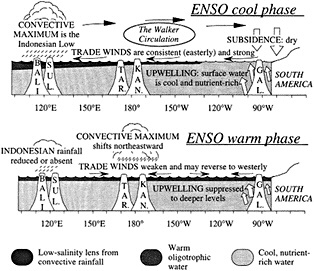
Figure 2
Schematic cross-section of equatorial Pacific showing major features of the warm and cool phases of ENSO in relation to selected sites where coral paleoclimatic reconstructions of ENSO are under way: Bali, Sulawesi, Tarawa, Kanton, and the Galapagos (after Cole, 1992).
ENSO intensify the upwelling of cool, nutrient-rich waters in the eastern Pacific and transport surface waters westward, generating a strong zonal SST gradient and an eastward slope in sea level.
Transition to the warm phase of ENSO may occur when the trade winds relax or reverse west of the date line, depending on surface ocean conditions. As the warm phase of ENSO begins, the western Pacific warm pool spreads eastward (Lukas et al., 1984; McPhaden and Picaut, 1990), and the Indonesian Low convective system migrates to the region near the date line and the equator. In the eastern Pacific, surface waters become warm and oligotrophic, as the thermocline deepens and warm waters move in from the west. Trade winds remain weak and variable as a result of the diminished zonal SST gradient. Dramatic shifts in precipitation patterns occur across the entire tropical Pacific, from South America to southeast Asia, in response to Indonesian Low migration and the development of convection over newly warmed ocean regions.
Frequency-domain analyses of climate data that span the past four decades indicate that ENSO operates on three fundamental time scales. The annual cycle sets the phasing of ENSO anomalies; the evolution of ENSO extremes appears phase-locked to the annual cycle (Rasmusson and Carpenter, 1982). Several aspects of ENSO variability, including SST, winds, rainfall, and sea level pressure (SLP), also possess a quasi-biennial pulse that varies in intensity throughout the instrumental record (Trenberth, 1980; Rasmusson et al., 1990; Barnett, 1991; Ropelewski et al., 1992). Finally, ENSO warm extremes recur approximately every 3-7 years, lending a ''low-frequency" beat to the spectrum of ENSO variability (Rasmusson and Carpenter, 1982; Rasmusson et al., 1990; Barnett, 1991; Ropelewski et al., 1992). Recent analyses of multi-decadal records of Pacific climate suggest that ENSO variability may also experience significant decadal-scale shifts (Elliott and Angell, 1988; Cooper et al., 1989; Trenberth, 1990). Such a shift is evident over the interval between 1977 and 1988, which exhibited no strong cool anomalies (Trenberth, 1990; Kerr, 1992).
The impacts of the Southern Oscillation both within and beyond the tropical Pacific fluctuate on a multi-decadal time scale (Trenberth and Shea, 1987; Elliott and Angell, 1988; Cole et al., 1993; Michaelsen and Thompson, 1992; Rasmusson et al., 1995, in this volume). During the first 20 years of this century, for example, the interannual pulse of the Southern Oscillation was strong and highly correlated with climatic records both within the tropical Pacific and in sensitive teleconnected sites. The subsequent three decades, however, witnessed a general decline in the correlations among Pacific climate variables and between Pacific climate and teleconnected sites. Elliott and Angell (1988) propose that these fluctuations may result from the migration of the centers of strongest coherent variability in the Southern Oscillation over the course of the present century.
Short Records Document Spatial Patterns of ENSO
Major dynamic features of ENSO variability include SST and upwelling anomalies in the eastern Pacific, and rainfall and wind anomalies in the western Pacific. Coral records can be targeted to address variability in each of these parameters through careful site and tracer selection. Figure 3 (from Cole et al., 1992) compares six short (20-30 yr) monthly-to-seasonal-resolution records from corals that grew at sites spanning the equatorial Pacific: the Galapagos Islands (1°S, 89°W), Tarawa (1°N, 172°E), and Bali (8°S, 115°E). In the eastern Pacific, Galapagos corals yield records of d18O, Cd/ Ca, and Ba/Ca that track variations in upwelling and SST (Shen et al., 1987; McConnaughey, 1989; Lea et al., 1989). In Tarawa corals, d18O primarily monitors monthly variability in local rainfall, a consequence of the displaced Indonesian Low (Cole and Fairbanks, 1990; Cole et al., 1993), and Mn/Ca variations reflect wind reversals associated with especially strong ENSO warm extremes (Shen et al., 1992b). In Bali, the migration of the Indonesian Low causes drought during ENSO warm extremes; coral d18O shows moderate
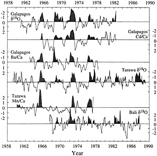
Figure 3
Comparison of short proxy records from corals that grew at three sites across the Pacific. (From Cole et al., 1992; reprinted with permission of Cambridge University Press.) All records are presented in units of standard deviation. Dark shading denotes recognized ENSO warm extremes (Quinn and Neal, 1992); lighter shading indicates conditions similar to the warm phase of ENSO at individual sites. These records target distinct components of the ENSO system; together they indicate both the Pacific-wide extent of ENSO extremes and the potential for the reconstruction of subtle patterns of spatial variability in ENSO. Periods of anomalies similar to ENSO warm phases but not recognized by Quinn and Neal (1992) occur in most records in 1963 and 1979-1980.
sensitivity to these fluctuations but probably includes a significant SST component as well.
Overall, these records monitor warm phases of ENSO consistently between sites. Cool phases of ENSO are best recorded by the Galapagos records and by the Tarawa d18O history. The Mn/Ca record at Tarawa appears to indicate changes in westerly wind intensity associated with strong warm phases, although it may not track variations in the intensity of easterly winds, and the Bali record does not show cool-phase anomalies consistent with the other coral records or with large-scale indices of Pacific climate.
Comparison of these records reveals patterns of spatial variability that are confirmed by concurrent instrumental records. For example, during 1979-1980, most of the Pacific experienced conditions similar to a weak ENSO warm anomaly. Although this year is not generally recognized as a major event (sensu Quinn et al., 1987), other studies have documented unusually warm SSTs and rainfall in the central Pacific during that time (Donguy and Dessiers, 1983). In 1977, the warm extreme of 1976 intensified in the western Pacific but decayed more rapidly into cool-phase conditions in the eastern Pacific. Variations in intensity of anomalies are also reflected in the coral data and generally confirmed by climatological data. In 1963 and 1969, for example, weak anomalies in the Tarawa d18O record are not concurrent with anomalies in the Mn/Ca record, which is consistent with observations of rainfall increases but no wind reversals at Tarawa. Cole et al. (1992) discuss these patterns in greater detail. This proxy intercomparison demonstrates that coral paleoclimatic tracers monitor large-scale ENSO anomalies across the entire Pacific basin, both warm and cool, and that they can also discern relatively subtle patterns of spatial variability and anomaly intensity in specific climatic and oceanographic parameters.
Calibration of Geochemical Tracers in a Galapagos Coral
In Galapagos corals, several tracers hold promise for reconstructing the SST and upwelling variability that define the eastern Pacific signature of ENSO. Shen et al. (1992a) measured parallel records of Cd/Ca, Ba/Ca, Mn/Ca, d18O, and d13C at quarterly resolution from a coral that grew at Punta Pitt, Isla San Cristobal, on the eastern side of the Galapagos archipelago. These records span the period 1936 through mid-1982. With the exception of Mn/Ca, all tracers show high correlations with SSTs measured at Puerto Chicama, Peru; for seasonal records, R falls between 0.51 and 0.65, and for annual averages, R ranges from 0.61 to 0.73. Even higher correlations are found between the tracers and the shorter SST record from Academy Bay, Galapagos, with seasonal R values ranging from 0.57 to 0.79 and annual values falling between 0.72 and 0.90. These tracers monitor slightly different aspects of the eastern Pacific ENSO signal: d18O tracks SST variability, Ba and Cd reflect the surface
concentrations (i.e., upwelling) of these nutrient-like tracers, and d13C probably responds to insolation variations, although this relationship is not constant for all coral d13C records from the Galapagos (McConnaughey, 1989).
Figure 4 compares the coral record of d18O anomaly from Punta Pitt with SST anomalies from Puerto Chicama and with an index of eastern-central Pacific SST anomalies (Wright, 1989). The d18O record captures most measured SST anomalies in these curves, both positive and negative. In certain cases where the d18O and Puerto Chicama records disagree (e.g., in 1980), the Wright SST index appears to corroborate the d18O record, suggesting that variability in the coastal SST record does not always represent conditions in nearby open ocean regions. Deser and Wallace (1987) have also noted that SSTs along the Peru coast occasionally become decoupled from large-scale variations in Pacific climate.
Cross-spectral analysis of the Punta Pitt coral records with records of Puerto Chicama SST indicate that correlations at the frequency bands associated with ENSO (about 2 and 3.8 years, in these records) reach values as high as 80 to 90 percent. Shen et al. (1992a) note that the observed degree of correlation, in both time and frequency domains, is truly remarkable, considering that these single proxy records derive from a site several hundred kilometers away from the coastal SST monitoring station at Puerto Chicama.
A Century of ENSO Variability in the Central-Western Pacific
In the western Pacific, ENSO variability is characterized by dramatic shifts in rainfall patterns associated with the migration of the Indonesian Low from northern Australia/ Indonesia to the region of the equator and the date line.
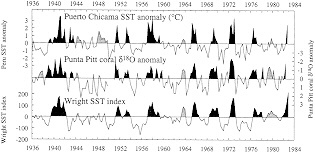
Figure 4
Plot of d18O anomaly from a Galapagos coral (Shen et al., 1992a) compared to SST anomalies measured at Puerto Chicama (Peru) and indexed over the eastern-central Pacific (Wright, 1989). Dark shading denotes recognized ENSO warm extremes (Quinn and Neal, 1992); lighter shading indicates conditions similar to the warm phase of ENSO at individual sites. Periods of anomalies similar to ENSO warm phases but not recognized by Quinn and Neal (1992) occur in all records in 1944, 1963, and 1979-1980.
Biweekly monitoring of surface ocean d18O at Tarawa Atoll demonstrates that at this site, rainfall causes a significant decrease in the d18O of the surface water in which corals grow (Cole, 1992). Coral d18O records from this site closely track these rainfall changes (Cole and Fairbanks, 1990; Cole et al., 1993). Our coral d18O record extends back to 1894 at monthly resolution, double the length of the instrumental record of Tarawa rainfall that began in 1946. Between 1976 and 1989, the Tarawa coral record suggests a period of increased rainfall that is unprecedented within this record. This apparent baseline shift is consistent with instrumental records from the Pacific (Trenberth, 1990; Kerr, 1992).
This d18O record correlates with large-scale indices of ENSO (Figure 5) at levels comparable to monthly instrumental records from individual Pacific stations, such as Tarawa rainfall and Darwin SLP. Monthly, seasonal, and annual d18O data linearly explain fractions of ENSO variance that are among the highest for any proxy record of ENSO (Cole, 1992; Cole et al., 1993). Despite the strong correlation between the coral and instrumental records of ENSO, the Tarawa d18O record does not capture the very strong ENSO warm anomaly of 1982-1983. Outgoing long-wave radiation measurements indicate that during that year the Indonesian Low moved much farther east than usual (Rasmusson and Wallace, 1983). Tarawa rainfall was not unusually intense at this time, and the coral d18O data reflect these conditions accurately. This anomaly that bypassed Tarawa is the only major ENSO extreme of the past century that the coral d18O record does not monitor, attesting both to the fidelity of the coral recorder and to the unusual nature of the 1982-1983 ENSO extreme. To reconstruct the full range of ENSO variability will require developing records from sites throughout the Pacific.
The coral record generally indicates warm and wet ENSO extremes during periods identified by Quinn et al. (1987) as "El Niño events" along the coast of South America. However, Figure 5 suggests exceptions to this correlation. In 1907, 1917, 1932, and 1943, Quinn et al. identify moderate or strong El Niño events, but neither the coral nor the instrumental indices of tropical Pacific climate indicate ENSO warm anomalies. In other years (e.g., 1946, 1963) the opposite pattern occurs; coral and instrumental indices demonstrate ENSO warm extremes that do not appear as moderate or strong in Quinn's most recent summaries (Quinn et al., 1987; Quinn and Neal, 1992), although these years were noted as weak anomalies in an earlier compilation (Quinn et al., 1978). Rasmusson et al. (1995, in this volume) have also noted, on the basis of instrumental climate records, that recurrence statistics derived from Quinn et al.'s "strong/very strong" events do not reflect basin-scale ENSO variability. Quinn et al. (1978, 1987, 1992) explicitly state that their index may not be entirely consistent with climatic records from across the tropical Pacific, such as the Southern Oscillation Index or central Pacific rainfall
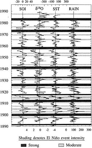
Figure 5
Comparison of the d18O measured in a Tarawa Atoll coral with large-scale indices of Pacific climate from Wright (1989). Shaded bars denote El Niño events identified by Quinn and Neal (1992) from historical information; strongest events are shaded most darkly (from Cole, 1992). Strong and moderate El Niño events in 1907, 1917, 1932, and 1943 have no counterparts in the instrumental or coral records, indicating anomalies localized to coastal South America in those years. The coral record indicates a shift to wetter conditions at Tarawa between 1976-1989 that is unprecedented in the past century.
histories, especially with regard to anomaly intensity. However, their compilation of El Niño events remains widely (if perhaps inappropriately) used as a history of large-scale ENSO variability. Both climatological and coral data from across the Pacific indicate that the Quinn index of El Niño events in coastal South America does not consistently track the state of the Pacific-wide ENSO system during the past century (Rasmusson et al., 1995, in this volume; Cole et al., 1993).
Frequency-domain analysis of the Tarawa d18O record suggests that interannual variance across periods of 1.9-2.5, 3.0, 3.6, and 5.6 years are highly coherent with large-scale ENSO indices; at these periods 80 to 90 percent of the variance in the Tarawa d18O record is linearly related to variance in the instrumental ENSO indices (Cole, 1992; Cole et al., 1993). These results, shown in Figure 6, fit into the general framework of studies that indicate biennial and low-frequency concentrations of variance in ENSO-related climatological data. With 96 years of coral d18O data, we can address the issue of whether the spectral signature of ENSO has changed over the period of our record.
We examine the distribution of variance among dominant periods over the length of the record by performing spectral analysis on a series of 30-year windows of d18O data, each shifted by 2 years from the previous. This evolutionary spectral analysis suggests that the variance spectrum of ENSO may have changed during the past century (Figure 7; Cole et al., 1993). Our 30-year intervals are too short to identify the specific frequencies noted above with statistical confidence, but this analysis suggests intriguing broad-scale changes in the variance spectrum of rainfall at Tarawa. Figure 7 maps the changing concentrations of variance at periods between 1 and 10 years over the past 96 years. In
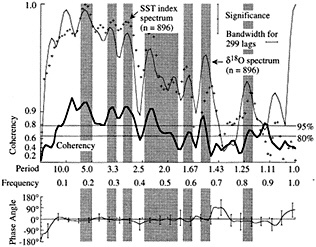
Figure 6
Cross-spectral comparison between SST index from Wright (1989) and Tarawa d18O record (Cole, 1992). Upper panel shows the variance spectra of the Tarawa d18O record (solid fine line) and the Wright SST index (plus symbols), plotted against frequency. The coherency between these records, which represents the degree of correlation between them as a function of frequency, is shown by the heavy line; the squared coherency gives the percent variance in common between the records. The lower panel shows the phasing of the records as a function of frequency. Shaded bars indicate frequency bands over which variance peaks are aligned; coherency is non-zero at more than 80-95 percent significance. At interannual periods characteristic of ENSO (here centered at 5.6, 3.5, 3.0, and 2.1 years), these records share at least 80 percent of their variance and are in phase. These results are consistent with cross-spectral analyses between the Tarawa record and other instrumental indices of ENSO (Cole, 1992).
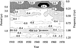
Figure 7
Evolutionary spectrum of variability in the Tarawa coral d18O record. (From Cole et al., 1993; reprinted with permission of the American Association for the Advancement of Science.) This figure maps the shifting distribution of variance (in units of log spectral density) in the Tarawa d18O record throughout the present century. The information in this figure derives from spectral analysis of overlapping 30-year intervals of monthly d18O data, offset by 2 years. Results are plotted against the midpoint of the analysis interval. The upper error bar on these values is 0.36 and the lower bar is 0.22. Overall, this figure suggests a change in the behavior of ENSO between about 1930 and 1950, with greater power at 5-to-6-year and annual periods and reduced power at 3-year periods.
the early part of this century, interannual variance at Tarawa is concentrated at periods longer than 2.5 years, and the annual cycle is moderately strong. In the interval between 1930 and 1950, annual variability intensifies and a minimum in variance occurs at the 3-year period. During this interval, in which the Southern Oscillation was thought to have generally weakened (Elliott and Angell, 1988), annual variance has approximately the same strength as low-frequency variability. Between 1955 and 1985, a strong variance peak centered at about 3.3 years reappears, and the annual cycle is at its weakest. Overall, these results imply a mode of ENSO behavior between about 1930 and 1950 that differs from preceding or subsequent periods.
Climatological studies that span only the most recent decades generally note that in the central-western Pacific, annual variability is secondary to interannual variance in many climatic parameters. Our coral record suggests that the strength of the annual cycle has varied at Tarawa, perhaps reflecting changes in the seasonal influence of either the southeast Asian monsoon or the eastern Pacific cool tongue. The annual cycle at Tarawa has been particularly weak since about 1950, coincidentally the time at which many instrumental records from the tropical Pacific begin. Evolutionary spectral analysis of the Tarawa d18O record highlights the limitations of using a short climatological data set to evaluate relative concentrations of variance at characteristic ENSO frequencies. At Tarawa, changes in the relative concentrations of annual and interannual variance have occurred over the past century; they may relate to overall shifts in the strength of the Southern Oscillation or to changes in the location of maximum expression of ENSO system variability. Our coral results require confirmation by further studies; additional records from the central and western tropical Pacific will allow us to draw more specific conclusions about the nature of these changes.
Urvina Bay Records: 400 Years of Oceanic Variability in the Eastern Pacific
A sub-aerially exposed Galapagos coral reaching nearly 400 years in age offers the opportunity for long paleoceanographic reconstructions from the eastern Pacific. In 1954 a portion of Urvina Bay, on the west coast of Isabela Island, was tectonically uplifted, exposing several square kilometers of pristine coral reef and marine shelf (Colgan and Malmquist, 1987). The oldest of the uplifted corals has been sampled for paleoenvironmental purposes. Dunbar et al. (1991, 1994) present a 371-year, annual-resolution record of coral d18O and growth rates from Urvina Bay that indicates significant decadal-scale variability in SST. Variance peaks at 11- and 22-year periods hint at sunspot modulation of eastern Pacific climate, although a direct link between sunspot activity and eastern Pacific upwelling remains to be established.
A 380-year annual record of Mn/Ca from the same coral has also been developed (Shen et al., 1991). Short segments of seasonal-resolution data throughout this record indicate the persistence of seasonal upwelling variability since the mid-seventeenth century. Upwelling intensity is difficult to quantify with this tracer, however, due to the large-scale spatial gradients in surface water Mn content. A long-term decreasing trend in Mn/Ca may indicate oceanic or atmospheric processes. Linn et al. (1990) suggest that higher Mn/Ca ratios in seventeenth-century samples from this Urvina Bay coral may be explained by either increased trade-wind strength or increased influence of Panama Basin water masses at that time. However, the possibility of an accumulating diagenetic Mn phase in this coral has not been eliminated (Shen et al., 1991).
Additional work in progress on this coral includes high-resolution d18O records and records of other trace elements. Results from this site will be placed in a regional perspective through ongoing studies of coral records that attain ages of 100-400 years from elsewhere in the eastern Pacific, including the Gulfs of Panama and Chiriquí, the Costa Rican islands of Caño and Cocos, and the southern Gulf of California (Linsley et al., 1991, 1994; Dunbar et al. 1993, 1994). Analysis of variability in the Pacific-wide ENSO system over the past several centuries will require the comparison of these eastern Pacific records with long reconstructions
in progress from central and western Pacific sites such as Tarawa Atoll, Sulawesi, and Kanton Island.
CONCLUSIONS
Isotopic and trace-metal records from massive corals offer the opportunity for focused retrospective monitoring of tropical climate processes, including many of the key dynamic features of the ENSO system. Short records from sites throughout the tropics have shown the sensitivity of various chemical tracers in coral skeletons to environmental variability. Recent application of these methods is beginning to yield insight into the past behavior of specific components of the global climate system. For example, extensive work with tropical Pacific corals indicates that coral proxy records not only capture the large-scale ENSO anomalies that recur interannually, but also track subtle patterns of variation in the intensity and spatial patterns of anomalies. Statistical comparisons in the time and frequency domains suggest that many Pacific coral records approach the utility of single-station instrumental records reconstructing large-scale ENSO indices. Evolutionary spectral analysis of a proxy ENSO record from a western Pacific coral suggests that the relative concentrations of variance at annual, biennial, and low-frequency periods has varied over the course of this century, perhaps in relation to fluctuations in the overall strength of the Southern Oscillation or to changes in the locations of centers of action of this system. Thus, the development of coral chemical records that span centuries will improve the canonical description of ENSO variability that is currently based on the instrumental record of only the past few decades.
Paleoclimatic records from remote tropical sites can yield substantive information on natural climate variability, offering insights not available from the limited instrumental record or even from skilled numerical simulations. Paleoclimatic records from corals capture the full range of natural variability, including decadal-scale shifts and changes in the dominant frequency components of climate variability. Furthermore, calibration of coral tracers over recent periods will provide the basis for developing records of tropical climate that extend into times of altered boundary conditions; such records offer a logical means of evaluating the sensitivity of tropical systems to global climate change.
ACKNOWLEDGMENTS
This report benefited greatly from careful reviews by Rob Dunbar and Clara Deser. Many participants in the Dec-Cen workshop provided helpful commentary, and we thank the National Academy of Sciences/National Research Council for their sponsorship of this event. We also thank the NOAA Paleoclimatology Program and the National Science Foundation for their support of this research.
Commentary on the Paper of Cole et al.
CLARA DESER
University of Colorado
Dr. Cole et al. have demonstrated that selected chemical records from corals at key locations in the tropical Pacific can yield an accurate history of ENSO variability. The coefficients of the correlations between the coral records and measured environmental variables exceed 0.7 or so on seasonal and annual time scales. Their study has also shown that a network of coral sites across the equatorial Pacific can be used to investigate the spatial characteristics of individual ENSO cycles.
The long (approximately 100-year) coral record at Tarawa in the western equatorial Pacific reveals changes in the frequency characteristics of ENSO during this century. Further insight into the dependence of ENSO on surface boundary conditions may come when the coral records are extended back several more centuries.
There may also be other applications for the coral records, such as monitoring the atmospheric heat sources over Indonesia, South America, and Africa.
Discussion
SOCCI: If the mean temperature rose substantially, would you have to get a new set of correlations to predict the coral's response to variations?
COLE: No, we don't expect the relationships we've found to change. The temperature dependence of d18O and the biogenic carbonates is pretty well established, and corals appear to have a very consistent response over a range of time scales and temperature levels. Similarly, the rainfall signal in coral d18O should not change, but the proportion of the coral signal due to rainfall rather than temperature changes could vary with changes in the mean state.
KEELING: Enfield's paper says that El Niños tend to be spaced further apart for a while and then closer together for a while. Do you see anything similar to that, at least after 1890?
TRENBERTH: Dennis Shea and I analyzed the record for this century. We saw regular El Niño events early in the century, then a break with only the unusual one of 1939-1942, then since the 1950s more regular ones again, with a strong peak around 4 years.
RASMUSSON: I think these coral data are exciting stuff. I wanted to introduce a note of caution as regards Enfield's study, though. First, he didn't use his weaker data because he didn't trust them, but I wonder whether we can then trust his distinction between weaker and stronger. Second, he had only 8 to 10 events per century, which doesn't yield stable statistics. Third, when the events are compared over 120 years of basin-scale historical data, there is correspondence in only about half of them.
I have two questions for you, Julie: Will you be comparing Kanton and Tarawa, and when will you extend this record to 300 years?
COLE: Starting with the second question: as soon as I can find corals that old. We know they exist, and we'll be looking at less settled islands near Tarawa as soon as we get funding. As for Kanton corals, Rick Fairbanks has just collected some, and they should be analyzed soon.
MOREL: It will be fascinating to see what corals will show for very different climate conditions. When do you think it will be possible to have information reflecting, for example, ENSOs from past glacial ages?
COLE: Naturally, that will depend on the funds available; we have proposals out already. Rick drilled a series of cores off Barbados that go back about 30,000 years, and found many decade-to century-long time series. We need similar cores from locations in the Pacific to answer that kind of question.
TRENBERTH: There's a lot we can learn from corals on the longer time scales, though the absence of the 1982-83 El Niño from the Tarawa record underlines the importance of using more than one site. I was glad you looked at the coherence of the signal at different frequencies to determine the source of the relationship; I wish more paleo people would. It will be critical on the longer time scales.
CANE: Satellite data is too short-term to tell us much of anything on the time scales we're interested in, and even the instrumental record can't give us more than a few realizations of anything on time scales of a decade or more. The coral records are exciting, particularly since our ability to interpret what comes out of them as a geophysical signal seems to be much greater than for any other kind of proxy data available to us. Within the next few years I think we'll be able to get some ideas about what the natural variability has been like over the last few centuries, and even why ENSO is irregular.
MUNK: I confess I was disappointed in your 300-year limit: I was hoping to go back to the Devonian.
COLE: At present we can't go back to the Devonian continuously. Also, with the older material you have the problem of diagenesis, during which the oxygen in the skeleton is exchanged. But by patching together records we should be able to get some ideas about older time periods. For example, corals 88 and 125 thousand years old preserve a nice seasonal d18O cycle.
PHILANDER: Wasn't there a recent article in Science reporting coral records of much colder SSTs 9 or 10 thousand years ago?
COLE: Yes, by Warren Beck et al. They use an exciting high-precision technique, measurement of strontium/calcium ratios by thermal-ionization mass spectrometry. The strontium seems to be a close recorder of a pure temperature signal, so it can be used to separate the patterns of variability in the combined rainfall and temperature change we usually see in the tropics.
LEHMAN: Another possible application of this coral work is as an indicator of how much the tropical moisture pump spikes the surface of the ocean with rainwater, on time scales much longer than El Niño events. That will be very important.
COLE: In a 1960 paper Colin Ramage said that something like 50 percent of tropospheric water vapor comes from the equatorial Pacific and the Indonesian area. If this system is responding to conditions such as changes in sea level, small changes in this region might be amplified by positive water-vapor feedback.
LINDZEN: For the lower 2 or 3 km of the atmosphere the water vapor is largely determined by temperature, whereas the greenhouse in the tropics is almost entirely determined by water vapor above 3 km. That's only a few percent of the total, and decoupled from the boundary besides. I don't think the surface budget will give you much insight there.
COLE: But upper-level water vapor must originate from the surface initially. And large changes at lower levels may have significant impact.
RASMUSSON: Julie, did you have problems related to the 198283 coral mortality, or tectonic shifts?
COLE: In the Galapagos, 1982-83 caused a lot of coral damage and also made possible an amazing amount of bioerosion. There aren't many long coral records left there. The uplifts resulting from tectonic activity have given Rob Dunbar and Glen Shen some useful samples, one of them the longest existing coral paleoclimate record.
Natural Variability of Tropical Climates on 10- to 100-Year Time Scales: Limnological and Paleolimnological Evidence
F. ALAYNE STREET-PERROTT1
ABSTRACT
A lake is a passive hydrological storage. It varies in depth and surface area in response to changes in its atmospheric, land-surface, and subsurface fluxes of water. Provided that groundwater inflows and outflows are negligible, it can be modeled as a simple, low-pass signal filter with a characteristic time constant (e-folding time) te. For closed lakes, which lack surface outlets and lose water solely by evaporation, te varies from about 1.5 to at least 350 years. For open lakes regulated by surface outflow, te is generally shorter, of the order of 10-2 to 5 years. Small, shallow closed lakes or large open lakes with te equal to 5 to 10 years provide good records of both interannual-to-decadal and longer-than-century variations in climate, whereas large, closed lakes with te greater than 50 years provide the best coverage over the intervening range of decade-to-century fluctuations. However, allowance must be made for characteristic time lags in the response of lakes to climatic fluctuations of period less than 2 te. This paper illustrates the response of tropical lakes to variations in ocean-atmosphere interaction over the Pacific, Indian, and Atlantic oceans during the period of limnological observations, and concludes with examples of paleolimnological evidence for century-scale droughts in southern Africa and the tropical Americas.
INTRODUCTION
In areas where humans have not significantly perturbed the water budget, fluctuations in the water level and surface area of lakes provide a physical indicator of climate on time scales of 10-1 to 106 yr. This paper has three aims: first, to summarize the general principles governing the response of lakes to variations in aridity, focusing on the decade-to-century time scale; second, to present examples of the behavior of tropical lakes over the last few centuries; and third, to comment on the links between the observed hydrological record and air-sea interaction over the tropical oceans, since the time scale highlighted here is longer than the response time of the atmosphere on its own. It concludes by emphasizing the need for a more coordinated approach to data collection and storage.
THE RESPONSE OF LAKES TO VARIATIONS IN SURFACE WATER BALANCE
The general water balance of a lake can be written as
where V is the lake volume, R and D are the surface runoff and discharge rates into and out of the lake, EL and PL are the evaporation and precipitation rates over the lake surface (in units of depth per unit time), AL is the lake-surface area, and Gi and Go are the groundwater inflows and outflows from the lake.
For closed, sealed lakes, defined as those that lack a surface outflow and for which the subsurface fluxes are negligible, equation (1) reduces to
At equilibrium, dV/dt = 0, and the equilibrium lake-surface area ALe is determined by (EL - PL) and R, which reflect the surface water balance over the lake and its surrounding catchment, respectively. Hence,
At equilibrium, the ratio of the lake-surface area ALe to the total catchment area AC (including the water surface) is given by
where C is a dimensionless index dependent only on R, EL, and PL (Mason et al., 1994):
On time scales longer than a year, R may be approximated by the expression
where AB is the area draining into the lake (excluding the water surface), and PB and EB are, respectively, the mean precipitation and evapotranspiration rates over the basin (in units of depth per unit time). Since by definition AC = AL + AB, C can now be rewritten as follows:
C is an inverse measure of aridity, ranging from near 0 in extremely arid conditions (small P and large E) to a theoretical maximum of 1 in very humid climates.
So far, only the equilibrium case has been considered. The response of the area of a closed, sealed lake to a perturbation in its inputs or outputs is determined by its characteristic response time (e-folding constant) te, defined as the time taken to reach a fraction (1 - 1/e), or 63 percent, of the total change in area. The response time te is given by
where L is lake level (Mason et al., 1985, 1994). Values of te calculated by Mason et al. (1994) for modern closed lakes vary from 1.5 to 350 years. te is greatest for extensive, steep-sided lakes in relatively moist climates, such as Lake Malawi in the historical past (see below).
For an open lake (a lake possessing an outflow) with negligible groundwater fluxes,
(Hutchinson, 1975). Calculated values of te for open lakes are in general much smaller than those for closed lakes, varying from 10 -2 to about 5 years (Mason et al., 1994).
The theoretical response of a closed, sealed lake to small perturbations in the aridity index C with time is summarized in Figure 1 (after Mason et al., 1994). Three simple types of change in C are illustrated: a step increase or decrease, a "spike" (short-lived fluctuation), and a sinusoidal oscillation of period p. A step increase (shown in curve a) or decrease (curve b) in C results in an asymptotic approach of lake area (or level) to its new equilibrium value over a time span dependent on te. A spike produces a rapid increase (curve c) or decrease (curve d) in lake area (or level), followed by a slower, asymptotic recovery. In contrast, a sinusoidal oscillation in climate produces an oscillating response with a phase shift dependent on the relative magnitudes of p and te. For low-frequency (LF) variations in climate of period p ![]() 2pte, the lake is approximately in equilibrium and exhibits negligible phase shift (curve e). For high-frequency (HF) variations of period p
2pte, the lake is approximately in equilibrium and exhibits negligible phase shift (curve e). For high-frequency (HF) variations of period p ![]() 2pte, the lake lags the variations in climate with a phase shift of -p/ 2 (curve f); the maximum and minimum rates of increase in area (or level) correspond to the maxima and minima in C, respectively (Mason et al., 1994). For practical purposes, the limits of the LF and HF bands can be taken as p > 20te and p < 2te. In theory, it should be possible to invert a time series of water-surface area or water level derived from a lake with known characteristics to obtain a record of variations in C (I. M. Mason, pers. commun.).
2pte, the lake lags the variations in climate with a phase shift of -p/ 2 (curve f); the maximum and minimum rates of increase in area (or level) correspond to the maxima and minima in C, respectively (Mason et al., 1994). For practical purposes, the limits of the LF and HF bands can be taken as p > 20te and p < 2te. In theory, it should be possible to invert a time series of water-surface area or water level derived from a lake with known characteristics to obtain a record of variations in C (I. M. Mason, pers. commun.).
In summary, a lake acts as a simple, low-pass signal filter with a characteristic time constant te. A wide range of lakes can act as climatic indicators on the decade-to-century time scale, although not necessarily over the whole range. Small, shallow, closed lakes or large, open lakes
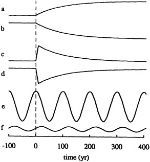
Figure 1
Theoretical response of the area AL of a closed sealed lake (vertical axis) to simple variations in the aridity index C with time (from Mason et al., 1994). (a) and (b) show the response of a lake with equilibrium response time te = 100 yr to a 10 percent step increase and decrease in C, respectively. (c) and (d) show the response of the same lake to a "spike," a 100 percent change in C that lasts for 10 years and then reverts to the previous value. (d) and (e) show the response of the lake to a sinusoidal variation in C of amplitude 10 percent. Curve (e) is for a lake with te = I yr, showing negligible phase shift, and representing the equilibrium response in the LF band. Curve (f) is for a lake with te = 100 yr, giving a phase shift of -p/2, as an example of the response in the HF band.
with te equal to 5 to 10 years potentially provide a good record of interannual to decadal fluctuations (their respective HF band). They should also exhibit negligible lag with respect to secular (LF) climatic variations. Large, closed lakes with te greater than 50 years can provide good coverage of decade-to-century (HF) variations. Whenever a response in the HF band is considered, however, allowance needs to be made for a phase shift of -p/2 with respect to the climate signal.
EVIDENCE FOR PAST FLUCTUATIONS IN LAKE LEVEL AND SURFACE AREA
Time series of lake levels have traditionally been compiled from observational, historical, or paleolimnological (geological) data (Street-Perrott and Harrison, 1985). Few lakes, even in developed countries, possess instrumental (gauge-board) records extending back before A.D. 1875. In some cases, however, historical observations of the emergence or drowning of specific landmarks permit lake-level time series to be extended for several centuries further back, at least in outline (de Terra and Hutchinson, 1934; Street-Perrott and Harrison, 1985; O'Hara, 1993).
In data-poor regions, or for the period before the start of reliable historical observations, high-resolution paleolimnological studies provide qualitative and, in some cases, quantitative information about past variations in lake depth and area, based on direct dating of former shorelines, or analyses of stratigraphical, geochemical, and paleoecological data from sediment cores and surface exposures (Street-Perrott and Harrison, 1985). The time resolution of these studies, however, is dependent on the dating framework. The most precise data should in principle be obtainable from lakes with finely laminated mud, such as Lake Turkana, Kenya (Halfman and Johnson, 1988); however, these are generally rare in the tropics.
Recent studies at the Mullard Space Science Laboratory, University College London, have established the feasibility of measuring variations in lake level by satellite radar altimetry (Mason et al., 1984, 1990) and variations in lake area with imaging instruments such as the NOAA Advanced Very High Resolution Radiometer (AVHRR) or the Earth Resources Satellite-1 (ERS-1) Along-Track Scanning Radiometer (Harris and Mason, 1989; Mason et al., 1990; Harris et al., 1992). The overall accuracy is expected to be around ±0.25 m for water level and 1 percent for surface area (Mason et al., 1990). Figure 2 shows the variations in area of the closed Lake Abiyata, Ethiopia (7°N) (te ca. 4 to 9 years) between 1985 and 1991, derived from AVHRR images (Harris et al., 1992).
EXAMPLES OF LAKE BEHAVIOR OVER THE LAST TWO MILLENNIA
The Influence of the El Niño/Southern Oscillation (ENSO) System
Lake Titicaca (16°S) is a large, open lake, 8,100 km2 in area, situated at an altitude of 3,812 m above sea level in the Altiplano of Peru and Bolivia. The equilibrium response time te of the lake is probably less than 5 years. It is fed mainly by tropical summer precipitation. Wet (dry) summers in the altiplano are characterized by a poleward (equatorward) displacement and weakening (strengthening) of the mid-latitude upper westerlies over South America (Kessler, 1974). High water levels were observed in the 1920s, 1930s, 1950s, 1960s, late 1970s, and late 1980s, with low levels in the 1910s and 1940s (very marked) and around 1970 (Figure 3) (Kessler, 1974; Künzel and Kessler, 1986; Martin et al., 1993).
The time series of the yearly rise (maximum minus previous minimum level) of Lake Titicaca between 1915 and 1981 was analyzed by Künzel and Kessler (1986) using maximum-entropy spectral analysis. They identified sig-
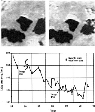
Figure 2
Water-level fluctuations of Lake Abiyata, A.D. 1984-1991, based on a time series of AVHRR imagery, together with sample images illustrating the appearance of the lake (center) in mid-1986 and late 1988 (From Harris et al., 1992; reprinted with permission of the European Space Agency.)
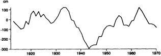
Figure 3
Measured water-level fluctuations of Lake Titicaca, A.D. 1912-1970. (Redrawn from Kessler, 1974; reprinted with permission of Dr. Kessler.)
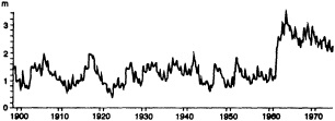
Figure 4
Measured water-level fluctuations of Lake Victoria, A.D. 1899-1974; (Redrawn from Vincent et al., 1979; reprinted with permission of Kluwer Academic Publishers.)
nificant spectral peaks with periods of 10.6 and 2.4 years. The former was assigned to the sunspot cycle and the latter to the quasi-biennial cycle. They also found a very weak period of about 4.7 years, which they ascribed to El Niño. More recent work suggests that both the quasi-biennial 2.4-year and lower-frequency 4.2-year cycles are associated with ENSO and the related variations in atmospheric angular momentum (Keppenne and Ghil, 1992; Dickey et al., 1992).
The Influence of Sea Surface Temperature Anomalies in the Indian Ocean
A lake that at least in part acts as an indicator of sea surface temperature (SST) anomalies in the Indian Ocean is Lake Victoria (1°S) in equatorial Africa. This is a very large, open lake (67,000 km2), with an equilibrium response time te of about 4.5 years (from data in Institute of Hydrology, 1985). Its water level curve for 1899 to 1978 shows the following features: oscillations about a stationary mean during the period 1899 to 1961; a step increase in lake level in 1961-1962; and an oscillating decline over the following 16 years (Figure 4) (Mörth, 1967; Vincent et al., 1979; Institute of Hydrology, 1985).
Spectral analysis of the lake-level record for 1899 to 1974 by Vincent et al. (1979) revealed only two significant peaks, at 10-13 years and 5-6 years, the first of which was attributed to solar variability in a famous paper by Brooks (1923). The record contains no power in the 2-to-3-year range; nor does it show any correlation with the Southern Oscillation Index (Vincent et al., 1979).
The sharp increase in lake level in 1961-1962 is an example of a ''spike" (Figure 4), although a preliminary inversion of the lake-level curve suggests that the climate over the Victoria catchment has not fully returned to its pre-1961 state (I. M. Mason, pers. commun.). The sudden rise in water level was the result of a remarkable rainfall anomaly over East Africa in August 1961 to January 1962, covering approximately 2.1 × 10⁶ km2. The peak occurred in November 1961 when rainfall over the Lake Victoria basin was almost 400 percent of normal (Flohn, 1987). Flohn has summarized evidence suggesting that this was merely the western end of a large, positive anomaly of SST, cloud, and rainfall covering about 6 × 10⁶ km2 of the western Indian Ocean, which is an extent similar to that of a typical ENSO warm pool or of the South Atlantic warming event of 1984 (Philander, 1986).
The Influence of the Atlantic (and Global) Sea Surface Temperatures
Pronounced decade-to-century-scale fluctuations in water balance have affected Lake Chad, situated at 13°N in the West African Sahel (Figure 5). This is a shallow, closed lake in a semiarid climatic zone; its area has fluctuated between about 1,950 and 26,000 km2 during the twentieth
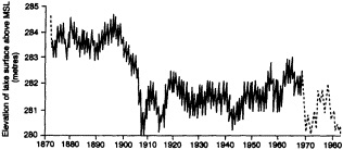
Figure 5
Water-level fluctuations of Lake Chad, A.D. 1870-1982, based on historical and instrumental data. (Adapted from Sikes, 1972, and updated by Thambyahpillay, 1983; reprinted with permission of Methuen and Co. and the University of Maiduguri.)
century (Thambyahpillay, 1983; G. Wells, pers. commun.). Over the past 40 years, its characteristic response time te has varied from less than 1 year in 1985 to a maximum of 7.7 years in 1954-1969, when it covered an average of 21,520 km2 (Mason et al., 1994). Note, however, that a small component of seepage loss, approximately 5 percent of the water budget (Roche, 1977), has been ignored in making these estimates. The lake-level curve from A.D. 1900 onward lags the instrumental record of sub-Saharan rainfall (Nicholson, 1985) by a year or two at most.
The reconstructed Lake Chad water-level curve for the last millennium (Figure 6) shows large fluctuations of 20 to more than 100 years' duration. Particularly high levels were recorded during the twelfth to fourteenth and the seventeenth centuries.
On the time scales of the last 100 and the last 10,000 years, fluctuations in Sahelian rainfall have been attributed to large-scale changes in SST fields. Following earlier work by Lamb (1978) and Lough (1986), Folland et al. (1986) and Parker et al. (1988) showed that twentieth-century droughts in the Sahel were significantly correlated with cold SST anomalies in the northern oceans, particularly the North Atlantic, and warm anomalies in the southern oceans, particularly the South Atlantic and the Indian Ocean. This
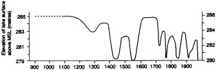
Figure 6
Water-level fluctuations of Lake Chad, A.D. 900-1980, reconstructed from a combination of stratigraphic, palynological, and historical evidence. (Redrawn from Maley, 1981; reprinted with permission of ORSTOM Editions.) Due to progressive sedimentation, two elevation scales are required; the left-hand one refers to the earlier part of the record and the right-hand one to the later part.
hemispherically asymmetrical anomaly pattern, which also characterized important low stands of Lake Chad on the millennial time scale, was ascribed by Street-Perrott and Perrott (1990) to a reduction in the northward heat transport in the Atlantic by the global thermohaline circulation. There is as yet no evidence to determine whether or not drought episodes within the last millennium can be explained by the same mechanism.
Examples of Droughts Lasting Several Centuries
The paleolimnological record provides examples of prolonged climatic fluctuations that have had profound significance for human communities in the tropics. For example, Lake Malawi (12°S), a large rift lake (28,750 km2) in equatorial Africa, has experienced variations in water level of at least 120 m vertical amplitude during the last few centuries (Owen et al., 1990). From A.D. 1860 onward, it fluctuated between 469 and 476 m above sea level. It was open throughout this period, with a response time te of about 3 to 8 years (R. Crossley, pers. commun.), apart from 1915 to 1935 when it ceased to overflow (Beadle, 1974). Between A.D. 1390 and 1860, however, there was a prolonged period of very low lake levels, represented by a widely traceable erosional unconformity and significant changes in diatom (algal) assemblages. During this low stand, the lake must have been closed, probably with a response time te much greater than 100 years. A rich oral tradition confirms that very low levels prevailed during the late eighteenth and early nineteenth centuries. Hydrological modeling by Owen et al. (1990) suggests that a reduction in rainfall of 40-50 percent, lasting for 100-150 years, could produce the required drop in lake level. The causes of such a prolonged anomaly remain uncertain, but probably involve large-scale oceanographic changes in the Indian and Atlantic Oceans.
An anomaly of similar duration is recorded by Lake Pátzcuaro (Mexico, 20°N) (O'Hara, 1992; Metcalfe et al., 1994). Lake Pátzcuaro is a small, closed lake with a modern te value of 22 years (from data in O'Hara, 1992). Sediment cores from the lake testify to a prolonged low stand, dated A.D. 800-1200. Low levels affected at least two other climatically sensitive lakes in the central Mexican highlands between A.D. 650 and 1200. This suggests that drought stress may have been a factor in the collapse of the great city of Teotihuacán (Basin of Mexico) and possibly of the Classic Maya ceremonial centers as well (Metcalfe et al., 1994; Hodell et al., 1995).
In contrast, isotopic investigations of Wallywash Great Pond, Jamaica (Street-Perrott et al., 1993; Holmes et al., 1995) indicate that a prolonged period of heavy rainfall, possibly of temperate origin, was centered on A.D. 750. Wet conditions also prevailed at this time in Lake Miragoane, Haiti (Curtis and Hodell, 1993). Paleolimnological studies of small lakes in the equatorial upper Amazon
(Colinvaux et al., 1985) have revealed an episode of widespread flooding in the interval A.D. 650-1250. The overlap in time between these prolonged anomalies of differing sign in the West Indies, Mexico, and Ecuador, all of which were the most important of the last 3,000 years in their respective regions, suggests that they reflect a large-scale reorganization of the areas of moisture convergence and cloudiness over the tropical Americas, compatible with a slight southward displacement of the Bermuda High.
RECOMMENDATIONS FOR FUTURE MONITORING
Where lakes are concerned, unlike glacier termini and river flows, there is as yet no coordinated program of monitoring and data archiving on a global scale. Although monthly gauge-board measurements are very simple to make, they are commonly interrupted by large changes in water level that necessitate relocation of the monitoring site, and the data are stored, often in haphazard fashion, by a great diversity of regional or national agencies.
A lake integrates the water balance over its catchment area. In arid and semiarid regions in particular, lakes offer the potential of bridging enormous gaps in the network of conventional meteorological and hydrological stations. Moreover, significant changes in water level are predicted to occur over the next few decades in response to greenhouse warming (Cohen, 1986).
What is needed now is a global program of data collection and storage, making use of appropriate satellite technology to provide monthly coverage on a near-real-time basis. An effort in this direction has been initiated by the Mullard Space Science Laboratory, University College London, using the data transmitted by ERS-1 (I. M. Mason, pers. commun.). However, much more could be done to coordinate both the collection of conventional instrumental, historical, and paleolimnological data, and the development of automated data-acquisition systems for other satellites.
ACKNOWLEDGMENTS
I wish to thank Ian Mason, Rob Crossley, and Sarah O'Hara for their help in preparing this paper.
Decade-to-Century-Scale Variability of Regional and Hemispheric-Scale Temperatures
PHILIP D. JONES AND KEITH R. BRIFFA1
ABSTRACT
Variability is examined in three types of temperature data: mean hemispheric temperatures from the last 100 years, longer single-site temperature records, and millennium-long tree-ring reconstructions of summer temperature. The annual average warming, since the late nineteenth century, is of the order of 0.5°C for both hemispheres. The warming is more erratic in the Northern Hemisphere, with a slight cooling between 1940 and 1970. The Southern Hemisphere shows less variability, with a more monotonic warming trend in this century.
Longer European temperature records indicate that the warming of the twentieth century is not unusual compared to that of some decades in the late eighteenth century. In most European records the nineteenth century was cooler than the eighteenth, with the 1880s the coldest decade. Some of the warmth of the last 100 years, therefore, may reflect the unusually low starting point. Four millennium-long tree-ring reconstructions (Fennoscandia, northern Urals, Tasmania, and northern Patagonia) are studied. In only one of these is the twentieth century the warmest, but in the others it is one of the warmest. Warmer conditions have been reflected in three of the summer reconstructions in previous centuries, but never at the same time at all four locations.
INTRODUCTION
One of the main reasons put forward for our inability to detect the enhanced greenhouse effect is that the inherent natural variability of the climate system is sufficiently great to obscure the signal (Wigley and Barnett, 1990). Although the 0.5°C global warming that has occurred over the last 100 years is consistent with model predictions resulting from greenhouse-gas buildup over this time (Wigley and Raper, 1992), our poor understanding of natural climate variability on the decade-to-century time scale means that a large part, or even all, of the observed warming might have occurred anyway.
There are no climatic elements for which we have records long enough to fully define the characteristics of past decade-to-century climate variability. The longest and geographically most extensive measurements are of surface
temperature, precipitation, and pressure, but there are problems associated with even these records. Measurements have never been global in extent, nor as spatially uniform as required by statistical sampling theory (Madden et al., 1993; Trenberth et al., 1992). Furthermore, the expected signals of greenhouse-gas-induced changes (e.g., as predicted by modeling experiments) for precipitation and pressure are poorly understood for a variety of reasons (Barnett and Schlesinger, 1987; Wigley and Barnett, 1990).
In this paper we consider two aspects of temperature variability. First, we study hemispheric-mean temperature variability over the last 100 years. Second, in order to examine temperature variations over longer periods, we look at some long single-site and composite instrumental records, principally from Europe, and at the few millennium-long paleoclimatic reconstructions of summer temperature. Although imperfect, these long records currently represent one of our only methods of looking at century-time-scale variability with "real" data.
VARIATIONS IN HEMISPHERIC MEAN TEMPERATURE
Land Regions
Before about 140 years ago, instrumental temperature measurements were limited to Europe, parts of Asia and North America, and some coastal regions of Africa, South America, and Australasia. By the 1920s the only areas without instrumentation were some interior parts of Africa, South America, and Asia; Arctic coasts; and the whole of Antarctica.
Although incomplete, the coverage since 1850 allows the development of continental and hemispheric averages of temperature. Using compilations of homogeneous station records, Jones (1988) and Jones et al. (1986a,c) produced a gridded (5° latitude by 10° longitude) data set of surface air-temperature anomalies over land for each month since January 1851. The basic data were interpolated on a regular grid to mitigate the effects of uneven spatial density of the station network. Interpolating the station data in absolute degrees is not a viable option, since this would be affected by varying station numbers, different station elevations, and different formulae for calculating monthly averages. The use of anomaly values from a common reference period (1951-1970) overcomes these problems. A consequence of this procedure is that hemispheric-mean temperatures are expressed in relative rather than absolute terms.
Time series of hemispheric-mean seasonal and annual temperature anomalies are shown in Figure 1. The features exhibited by the two sets of curves have been discussed before (see, for example, Folland et al., 1990, 1992; Jones and Briffa, 1992; Jones et al., 1986a,c; Wigley et al., 1985, 1986). The differences in temperature between the second half of the record (1946-90) and the first half (1901-45) are listed in Table 1. The annual series for each hemisphere shows a warming of the order of 0.5°C since the late nineteenth century. The warming is considerably more erratic in the Northern Hemisphere, where a cooling of about 0.2°C clearly occurred between about 1940 and 1970 in all seasons except spring. In the Southern Hemisphere the warming is more monotonic, and there is no evidence of cooling after 1940.
The various seasonal curves in Figure 1 show considerable variation in periods of warming and cooling. The greater difference between seasonal trends over the last 140 years occurs over the Northern Hemisphere. In summer and autumn, the 1980s were barely warmer than the temperature levels of the 1930s and 1940s. In winter and spring the 1980s were clearly the warmest decade. All seasons except summer show the long-term warming evident in the annual data. In summer, the 1850s to 1870s were as warm as the most recent two decades. The cooling from the 1870s to the 1880s is the most pronounced feature of the summer
TABLE 1 Temperature Differences, 1946-1990 Average Minus 1901-1945 (land-only data)
|
|
Whole Year |
Jan |
Feb |
Mar |
Apr |
May |
Jun |
Jul |
Aug |
Sep |
Oct |
Nov |
Dec |
|
Northern Hemisphere |
|||||||||||||
|
ΔT(°C) |
0.14 |
0.14 |
0.22 |
0.20 |
0.28 |
0.24 |
0.16 |
0.07 |
0.06 |
0.07 |
0.06 |
0.11 |
0.21 |
|
σ(1901-90) |
0.23 |
0.47 |
0.52 |
0.43 |
0.32 |
0.27 |
0.23 |
0.23 |
0.23 |
0.24 |
0.31 |
0.36 |
0.45 |
|
σ(1901-45) |
0.22 |
0.46 |
0.54 |
0.36 |
0.31 |
0.29 |
0.24 |
0.26 |
0.25 |
0.26 |
0.35 |
0.38 |
0.50 |
|
σ(1946-90) |
0.22 |
0.48 |
0.49 |
0.48 |
0.28 |
0.20 |
0.20 |
0.18 |
0.20 |
0.21 |
0.26 |
0.32 |
0.38 |
|
Southern Hemisphere |
|||||||||||||
|
ΔT(°C) |
0.21 |
0.20 |
0.17 |
0.21 |
0.15 |
0.28 |
0.23 |
0.30 |
0.29 |
0.19 |
0.17 |
0.20 |
0.19 |
|
σ(1901-90) |
0.19 |
0.25 |
0.26 |
0.27 |
0.26 |
0.32 |
0.28 |
0.30 |
0.33 |
0.27 |
0.26 |
0.24 |
0.25 |
|
σ(1901-45) |
0.15 |
0.22 |
0.27 |
0.23 |
0.22 |
0.26 |
0.27 |
0.26 |
0.30 |
0.22 |
0.25 |
0.22 |
0.23 |
|
σ(1946-90) |
0.17 |
0.24 |
0.21 |
0.26 |
0.28 |
0.31 |
0.25 |
0.27 |
0.29 |
0.29 |
0.24 |
0.21 |
0.23 |
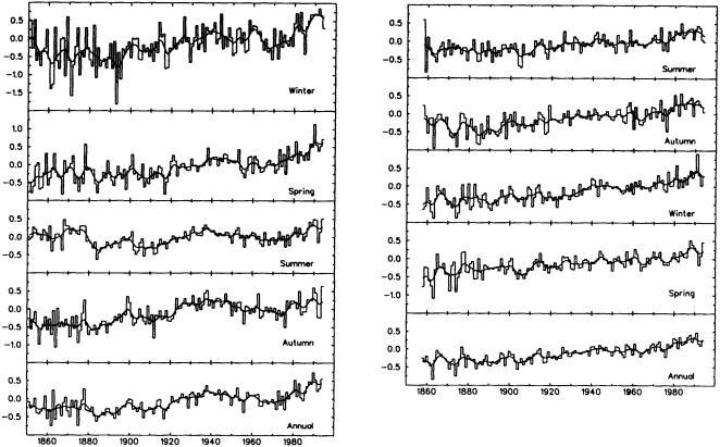
Figure 1
Surface air temperatures (land only) by season and year. Data are expressed as anomalies with respect to the 1951-1970 average. Smooth curves in this and subsequent plots were obtained by using a 10-year Gaussian filter. Left, Northern Hemisphere temperatures, 1851-1994; right, Southern Hemisphere temperatures, 1858-1994. Northern Hemisphere winters and Southern Hemisphere summers in this and subsequent figures are dated by the year in which the January occurs.
data. Over the Southern Hemisphere there is more agreement between the long-time-scale seasonal trends.
In both hemispheres, greater year-to-year variability is apparent during the nineteenth century. This increased variability is due to the sparser spatial coverage at that time. Although the estimates for individual years may be less reliable in the nineteenth than the twentieth century, the "frozen-grid" analyses undertaken by Jones et al. (1986a,c) indicate that the decadal-scale temperature fluctuations are reliably reproduced by the available data (for more discussion of this see Madden et al., 1993). The coolness of the 1880s compared with 1851 to 1880 in the Northern Hemisphere is, therefore, probably real. Thus, for the hemispheric temperature analyses of Hansen and Lebedeff (1987, 1988) and Vinnikov et al. (1990), who begin their analyses around 1880, warming rates measured over 1881 to 1990 are slightly greater than rates calculated over 1861 to 1990 (see also Folland et al. (1990, 1992) for more discussion of this point).
Land and Marine Regions
Since land represents only 29 percent of the area of the earth's surface, it is important to incorporate marine data into hemispheric averages if we want to get the "best possible" global series. Merchant and naval ships have taken weather observations and measured the temperature of the sea surface since the beginning of the nineteenth century. In the last 20 years, major international efforts have been made to transfer all of the climate data contained in ships' log books into computer data banks. One such compilation is the Comprehensive Ocean-Atmosphere Data Set (COADS) produced by NOAA workers at Boulder, Colorado (Woodruff et al., 1987). COADS contains about 80 million non-duplicated sea surface temperature (SST) observations. Another similar data set has been assembled by the U.K. Meteorological Office (Bottomley et al., 1990). Much of the data is common to both sets, but comparisons are under way to isolate the unique observations in each.
Unfortunately, as with land data, marine records are affected by inhomogeneities and errors. Correction schemes have been devised to adjust both marine air temperatures and sea surface temperatures for biases attributable to the method of measurement, time of day, etc. (see, e.g., Bottomley et al., 1990; Folland and Parker, 1990, 1991; Folland et al., 1990, 1992; Jones and Wigley, 1990; and Jones et al., 1991).
Land and marine temperatures may be combined in a number of ways. We describe below the Climatic Research Unit's combined data set, comprising the land temperatures discussed earlier and SST anomalies corrected for changes in measurement technique. The main change is from uninsulated-bucket to engine-intake measurements (and some insulated buckets) around the start of the 1940s. The SST correction scheme is discussed in detail by Jones and Wigley (1990) and Jones et al. (1991). The data, which are given as a set of 5° by 5° grid-box values, are anomalies from the 1950-1979 reference period. Where co-located land and marine grid data occur, the resulting value is the average of the land and marine components.
Annual and seasonal time series of hemispheric-mean temperatures, based on the combined data set, are shown in Figure 2. Detailed discussions of the features exhibited by the two sets of curves may be found elsewhere (see, for example, Folland et al., 1990, 1992; Jones and Briffa, 1992; Jones and Wigley, 1990). The differences in temperature between the second half of the record (1946-90) and the first half (1901-45) are listed in Table 2. In many respects the year-to-year and decadal-scale variations in Figure 2 are damped versions of those seen in Figure 1. There are, however, subtle differences. The greater nineteenth-century variability prominent in the land-only data is not as apparent in the land-plus-marine data. The cooling between 1940 and 1970 evident in the Northern Hemisphere land-only seasonal series is hardly apparent in the combined data. It is replaced by a period of little trend in 1940-1960, followed by a slight cooling from 1960 to the mid-1970s. Variability in the combined data set is now similar between the two hemispheres, whereas in the land-only data the Northern Hemisphere variability was clearly greater.
The intercorrelation between the two hemispheric combined series is remarkably high (for annual values between 1901 and 1990, r = 0.79). Some of this high correlation is due to coincident long-term trends, and the remainder is due to common high-frequency (year-to-year) variability. Some of the interannual correspondence derives from a response to the common forcing of the El Niño/Southern Oscillation (ENSO) phenomenon (Philander, 1983). Many of the years that are warm relative to the filtered curves in Figure 2 have been shown to be El Niño years or "warm event" years (Bradley et al., 1987b; van Loon and Shea, 1985). In contrast, many cold years, relative to the filtered curves, correspond to La Niña or "cold event" years (Philander, 1985). Using the Southern Oscillation Index (SOI) (Allan et al., 1991; Ropelewski and Jones, 1987), Jones (1989) has removed the ENSO influence from the hemispheric and global temperature series. The SOI explains about 25 to 30 percent of the high-frequency (less than 20 years) variations in hemispheric temperature anomalies
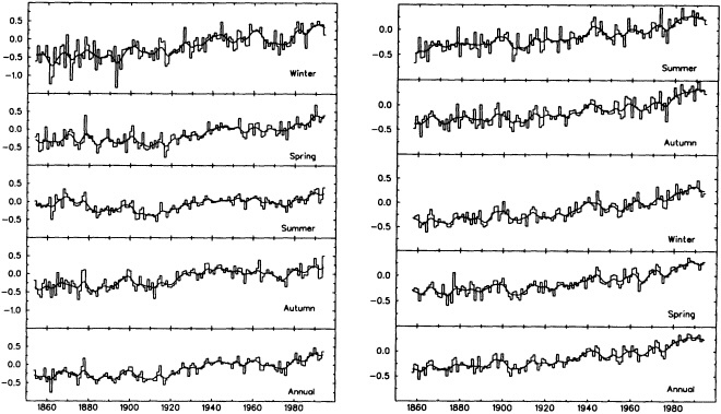
Figure 2
Northern Hemisphere (left) and Southern Hemisphere (right) surface air temperatures (land-plus-marine data) by season, 1854 to 1994. Data are expressed as anomalies from 1950 to 1979.
TABLE 2 Temperature Differences, 1946-1990 Average Minus 1901-1945 (land-plus-marine data)
|
|
Whole Year |
Jan |
Feb |
Mar |
Apr |
May |
Jun |
Jul |
Aug |
Sep |
Oct |
Nov |
Dec |
|
Northern Hemisphere |
|||||||||||||
|
ΔT(°C) |
0.23 |
0.24 |
0.28 |
0.30 |
0.30 |
0.28 |
0.23 |
0.19 |
0.18 |
0.17 |
0.14 |
0.17 |
0.28 |
|
σ(1901-90) |
0.21 |
0.32 |
0.36 |
0.32 |
0.26 |
0.23 |
0.21 |
0.20 |
0.20 |
0.21 |
0.24 |
0.26 |
0.35 |
|
σ(1901-45) |
0.20 |
0.29 |
0.35 |
0.27 |
0.24 |
0.22 |
0.20 |
0.21 |
0.21 |
0.22 |
0.27 |
0.28 |
0.36 |
|
σ(1946-90) |
0.16 |
0.31 |
0.32 |
0.30 |
0.19 |
0.14 |
0.15 |
0.13 |
0.15 |
0.16 |
0.19 |
0.21 |
0.28 |
|
Southern Hemisphere |
|||||||||||||
|
ΔT(°C) |
0.24 |
0.25 |
0.23 |
0.26 |
0.22 |
0.23 |
0.22 |
0.26 |
0.25 |
0.25 |
0.24 |
0.24 |
0.22 |
|
Δ(1901-90) |
0.20 |
0.24 |
0.23 |
0.23 |
0.22 |
0.23 |
0.23 |
0.24 |
0.25 |
0.23 |
0.21 |
0.20 |
0.23 |
|
σ(1901-45) |
0.14 |
0.21 |
0.21 |
0.19 |
0.16 |
0.17 |
0.18 |
0.19 |
0.19 |
0.15 |
0.18 |
0.16 |
0.19 |
|
σ(1946-90) |
0.17 |
0.21 |
0.20 |
0.21 |
0.22 |
0.23 |
0.21 |
0.20 |
0.24 |
0.22 |
0.18 |
0.17 |
0.21 |
|
Global |
|||||||||||||
|
ΔT(°C) |
0.23 |
0.25 |
0.26 |
0.28 |
0.26 |
0.26 |
0.23 |
0.22 |
0.22 |
0.21 |
0.19 |
0.20 |
0.25 |
|
σ(1901-90) |
0.19 |
0.25 |
0.27 |
0.26 |
0.22 |
0.21 |
0.19 |
0.19 |
0.20 |
0.19 |
0.20 |
0.21 |
0.26 |
|
σ(1901-45) |
0.16 |
0.22 |
0.24 |
0.20 |
0.19 |
0.18 |
0.17 |
0.17 |
0.18 |
0.16 |
0.21 |
0.20 |
0.24 |
|
σ(1946-90) |
0.15 |
0.21 |
0.23 |
0.23 |
0.17 |
0.16 |
0.15 |
0.14 |
0.16 |
0.15 |
0.14 |
0.15 |
0.21 |
about 25 to 30 percent of the high-frequency (less than 20 years) variations in hemispheric temperature anomalies. Removal of the ENSO influence produces data series that may assist in the early detection of greenhouse-gas-related trends (Nicholls and Katz, 1991; Wigley and Jones, 1981).
VARIATIONS IN LONGER RECORDS
Study of the hemispheric time series since 1850 allows the variability on the 10-to-30-year time scale to be investigated. Century-time-scale variability, however, can be considered only with records that span at least several centuries. In this section we examine some of the longest instrumental records available (principally from Europe) and some of the longest annually resolved proxy climatic reconstructions.
Longer Instrumental Records
The most detailed compilation of long-term instrumental climate data (both temperature and precipitation) currently available is that of Bradley et al. (1985). This compilation extended and improved on the previously available data sets by searching meteorological and other archives for published and manuscript sources of early instrumental records. An important aspect of the resulting compilation is that it contains details of the sources of all of the station data sets and, where possible, details of their long-term homogeneity (see Bradley et al., 1985; Jones et al., 1985, 1986b). Clearly, if one is to study climatic change, it is vital to ensure homogeneity of time-series data.
Figure 3 shows annual time series for 12 stations (for seasonal time series see Jones and Bradley, 1992). The time series are smoothed using a 10-year Gaussian filter to emphasize variations on decadal and longer time scales, and expressed as anomalies from the 1901-1950 period. The longest time series are restricted to the Northern Hemisphere between 40° and 64°N. All the series, except for Toronto, were considered homogeneous by Jones et al. (1985). We have included Toronto here because the extension of its record to 1770 (Crowe, 1992) makes it the longest such time series from North America. Urban warming is clearly evident from the 1880s on.
For the European sites, the warming of the twentieth century is not unusual compared to the longer record. The period encompassing the late nineteenth and early twentieth centuries is one of the coldest for Europe. Temperatures in the late twentieth century are only marginally higher than those during parts of the eighteenth century. The North American and Asian records clearly show long-term warming, but all these records begin much later than in Europe. Evidence from tree-ring reconstructions during the seventeenth and eighteenth centuries in western North America indicates conditions as warm as today's (Briffa et al., 1992b; Fritts, 1991).
Within-Region Similarities
A comparison of the long European records shows consistency on the decadal time scale, with strongly similar cool and warm decades since 1700. Cool decades are evident
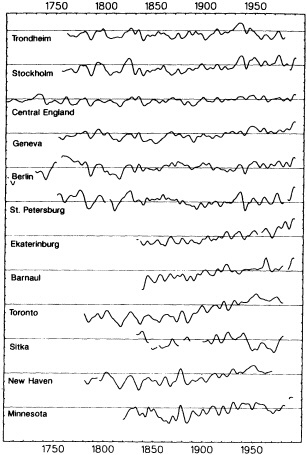
Figure 3
Low-frequency temperature variations at 12 selected sites having the longest records. Two records, central England and Minnesota, represent regional composite series rather than individual site records. The time series shown result from the application of a 10-year filter. Each tick mark on the vertical scale represents 1 °C. Data are expressed as anomalies from 1901 to 1950.
during the 1740s, 1780s, 1800s, and 1810s, and the late 1830s and 1840s. Warm decades are limited to the 1820s. Similar decadal similarities are seen in other regions. The two Asian records show cool decades during the 1830s and 1840s as in Europe. The four North American records show relative cold during the 1780s, 1810s, and 1830s, again similar to the European data, although warmth is indicated during the 1800s, the 1820s, and to some extent during the 1840s. The cold-warm-cold oscillatory pattern between the 1810s and 1830s is particularly striking in the New Haven and Toronto records in North America and at Stockholm and St. Petersburg in Europe.
Between-Region Similarities
Since 1850 the best-known difference between European temperatures and those in the rest of the hemisphere occurred during the early 1940s. At this time Europe was cold while the rest of the hemisphere was warm, at a level exceeded in magnitude only during the 1980s (Jones et al., 1986a). North American station records show warmth during the 1800s and 1840s, while European stations show cool conditions. Although some correspondence appears between warm and cool decades over the northern landmasses, more comprehensive regional studies of twentieth-century temperature variations over the Northern Hemisphere have shown that no one region can be said to be fully representative of hemispheric-wide temperatures (Briffa and Jones, 1993; Jones and Kelly, 1983). There is, therefore, no reliable short-cut method of estimating hemispheric or global temperatures on the basis of relatively few station records, at least on the decadal time scale, as has been tried by Groveman and Landsberg (1979). (Lack of longer-time-scale data prevents reaching a similar conclusion about estimating temperatures on century time scales.)
Proxy Records
Many methods are used to reconstruct past climates (see Bradley, 1985). Only a few, however, have the potential for providing records that can be resolved to an annual or seasonal level. Of those that can, the most widely used sources are documentary historical data, dendroclimatic data, and ice-core records (see Bradley and Jones, 1992). Documentary reconstructions are mainly restricted to Europe and Asia and to the period since about A.D. 1400 (see, e.g., Mikami, 1992). Few documentary reconstructions extend continuously over long time periods, the proxy temperature series for Switzerland from 1525 (Pfister, 1992), for China from 1470 (Wang and Wang, 1991), and for Iceland from 1590 (Ogilvie, 1992) being the longest. Documentary evidence probably represents the most reliable source of past climatic information on short time scales. The ability of some documentary indicators to faithfully record low-frequency climatic variations on time scales longer than the human life span (in particular a century or more) must be questioned, however.
Ice-core evidence is limited to high-latitude and high-altitude locations. Furthermore, few ice-core reconstructions of temperature are explicitly calibrated against instrumental time series, and there may be some ambiguity in interpreting the seasonality of the climate variations (Bradley and Eischeid, 1985; Thompson et al., 1986). When isotope-temperature relationships have been tested, the best correlations on the interannual time scale explain only about 25 percent of the temperature variance (Jones et al., 1993; Peel, 1992). Notwithstanding these points, ice cores represent important environmental information, and may be the principal means of reconstructing highly resolved long temperature series in terrestrial tropical areas (albeit at high elevations).
To illustrate the potential value of proxy data further, we concentrate on dendroclimatic reconstructions. Some of the longest represent "warm-season" temperatures in northern Fennoscandia, the northern Urals, Tasmania, and northern Patagonia (Briffa et al., 1990, 1992a, 1995; Graybill and Shiyatov, 1992; Cook et al., 1991, 1992; Villalba, 1990; and Lara and Villalba, 1993, respectively). Details of some of these reconstructions are given in Table 3 and in the caption of Figure 4. As noted in an earlier section, summer (particularly in the Northern Hemisphere) is the season that appears from the instrumental record since 1850 to be most atypical in its long-term changes (see also Briffa and Jones, 1993). Another potential limitation of dendroclimatic reconstructions is that they may not fully represent very-long-time-scale variability because of the need to transform original ring-width measurements into indices in order to minimize any potential bias in the mean chronology resulting from different ages of the constituent trees (Cook et al., 1990, 1995a). The apparent character, in terms of long-time-scale variability, of the different chronologies (and hence their climate reconstructions) depends on the longevity of the trees (and hence the length of the measurement time series), the ecology of the site(s), and the dataprocessing method used to remove the 'age effect'.
Figure 4 shows the reconstructions filtered with 20- and 100-year low-pass filters. Each of the series has been rescaled to represent anomalies from the 1901-1960 period. The importance of the different chronology-production methods is demonstrated in the upper halves of both panels in Figure 4, which show alternate reconstructions for each of two northern high-latitude regions: northern Fennoscandia, produced using the same ring-width and density measurement data (Briffa et al., 1990, 1992a), and the northern Urals region, based on different data sets (ring width only for June-July (Graybill and Shiyatov, 1992) and ring widths and ring density for May-September (Briffa et al., 1995)). Differences in the way the original growth measurements for the many individual trees were amalgamated within these chronologies has markedly affected the appearance of the long-time-scale variability in the resulting climate reconstructions. However, establishing the veracity, or true confidence levels, associated with the long-period fluctuations is extremely problematic.
Notwithstanding the methodological considerations, Figure 4 also shows that, compared to the southern series, the variance of the northern reconstructions is much greater. This may reflect the strong moderating influence of the southern oceans evident in the lower variance of the observational data in these regions. The explained variances in the southern reconstructions are also generally lower than those in the north (see Table 3). On the 20-year time scale, the temperatures for the two northern regions are largely out of phase between A.D. 1000 and 1200. In these comparisons, we use the two thicker curves for Fennoscandia and the Urals, which show the greater variability on decadal and longer time scales when Fennoscandia was warm and the Urals cold. After 1600, the two curves are more similar, both being cold through much of the seventeenth and the second half of the nineteenth centuries. The drop in temperatures in Fennoscandia began around 1580 and lasted to around 1750, whereas in the northern Urals the drop began earlier, the coldest period being from 1530 to 1670. Both series indicate cold summers around the end of the nineteenth century, although conditions were more severe in the Urals. The Fennoscandian series also shows protracted or relatively severe cold during the sixth, seventh, ninth, early twelfth, thirteenth, and early fourteenth centuries. On the 100-year time scale the Fennoscandian series shows generally continuous warmth exceeding that of the 1930s lasting from about 900 to 1100. Shorter warm periods also occurred during the 760s, around 1160, and notably in the early decades of the fifteenth century. The Urals series shows warmth in the thirteenth and fourteenth centuries, but on this time scale it does not exceed that of the twentieth century.
The nature of the Southern Hemisphere reconstructions is very different from that of those in the north. Low-frequency variability is conspicuously less. In Tasmania, the main feature of the entire reconstruction is a rapid increase in temperature since early this century. For northern Patagonia, the two series show less agreement with each
TABLE 3 Variance (r2) Explained by Calibration of Different Summer Temperature Reconstructions Based on Tree-ring Data (see Figure 4)
|
Region |
Reference |
Calibration Period |
r2 |
|
Northern Fennoscandia |
Briffa et al., 1990 |
1876-1975 |
0.51 |
|
Northern Fennoscandia |
Briffa et al., 1992a |
1876-1975 |
0.55 |
|
Northern Urals |
Graybill and Shiyatov, 1992 |
1881-1969 |
0.60 |
|
Northern Urals |
Briffa et al., 1995 |
1882-1990 |
0.68 |
|
Tasmania |
Cook et al., 1992 |
1938-1989 |
0.37 |
|
Northern Patagonia |
Villalba, 1990 |
1908-1984 |
0.42 |
|
Northern Patagonia |
Lara and Villalba, 1993 |
1910-1987 |
0.36 |
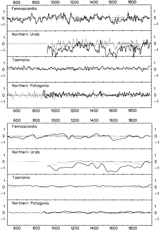
Figure 4
Variations in four of the longest tree-ring reconstructions of summer temperature. The reconstructions are for northern Fennoscandia (April to August; thick line, Briffa et al., 1992a; thin line, Briffa et al., 1990), northern Urals (May to September, thick line, Briffa et al., 1995; June to July, thin line, Graybill and Shiyatov, 1992), Tasmania (November to April; Cook et al., 1992), and northern Patagonia (December to February; thick line (Rio Alerce, Argentina), Villalba, 1990; thin line (Lenca, Chile), Lara and Villalba, 1993). Variations are shown in degrees Celsius after application of a 20-year low-pass filter (upper panel) and a 100-year low-pass filter (lower panel). For all series the zero line is 1901 to 1960.
other than might be expected. There is no evidence of any recent dramatic or unprecedented rise in temperature.
Taken together, the reconstructions for the two hemispheres show little coherence in century-time-scale variability. The most consistent features are the cool episodes from 1550 to 1650 and again between 1880 and 1910. The early period probably represents the coldest 100-year period of the last millennium, while the latter underscores the possibly exaggerated warming trends that may be estimated by calculating hemispheric trends beginning in the 1880s rather than the 1860s (see also Folland et al., 1990).
CONCLUSIONS
On the basis of the instrumental record, the 1980s was clearly the warmest decade. Warmth is evident in all seasons and in both hemispheres. There is evidence, clearer in the Northern Hemisphere, that the twentieth-century warming occurred in two phases, between 1920 and 1940 and since 1975. All seasonal curves, however, exhibit large decadal-time-scale variability superimposed on century-time-scale warming.
Longer single-site and composite instrumental records confirm the warming from the late nineteenth century on. The 250-year-long records from Europe show that the 1880s were the coldest decade, at least since 1700, so part of the warming since then may reflect this unusually low starting point. In most European records the eighteenth century was warmer than the nineteenth century.
In only one (the Northern Urals, Briffa et al., 1995) of the thousand-year dendroclimatic reconstructions is the twentieth century clearly the warmest century. In all of the other reconstructions, however, this century is one of the warmest. Warmer (summer) conditions occurred in previous centuries, but never at the same time at all locations. Clearly, a greater geographical spread of long paleoclimatic reconstructions is required; types of proxy evidence that cover seasons other than summer must be employed before the apparently unprecedented warmth shown in instrumental records of the twentieth century can be placed in a longer-term context.
ACKNOWLEDGMENTS
The authors thank Don Graybill, Ed Cook, Antonio Lara, and Ricardo Villalba for making the results of their long dendroclimatic reconstructions available. This research has been supported by U.S. Department of Energy's Atmospheric and Climate Division (Grant No. DE-FG02-86ER60397), the U.K. Department of the Environment (Contract No. PECD/7/12/78), and the E.U. Environment Programme (Grant EV5V-CT94-0500; DG12 DTEE).
Commentary on the Paper of Jones and Briffa
THOMAS R. KARL
NOAA National Climatic Data Center
I very much enjoyed reading this paper. I should just like to call your attention to some questions that were raised in my mind as I read through it.
First, there is the question of whether or not we can really adequately measure global-scale decadal fluctuation prior to about 1900. I am primarily concerned about the spatial resolution and spatial comprehensiveness of the data. I want to show one diagram to give you an idea of the types of errors that occur when you attempt to calculate global temperature trends and do not have complete global coverage of the phenomena. Starting out with complete global coverage and systematically removing data to calculate a trend over 10, 50, 150 years—removing it in a way that matches the historical coverage of the observations over both land and sea, of course—on a 10-year time scale you get standard errors that are over 1°C. The standard errors come down to perhaps 0.4°C to 0.6°C for 50 years; when you go out to 100 years, the standard errors are much smaller. There are also some significant biases that can creep into the record. This is cause for thought.
Another question I have is related to an issue Gene Rasmusson raised: Are we optimally using the data we have? Are 5- by 10-degree boxes the best way of calculating these global numbers? Is some kind of optimal averaging preferable? You get slightly different answers depending on how you go about the averaging.
My third point is the issue that Dr. Jones raised with respect to the very cool conditions during the 1880s, especially during the summer. You wonder not only about the spatial comprehensiveness of the data at that time, but also whether there could be some exposure problems.
Another question was raised in my mind by Dr. Jones's comment that decadal-scale temperature anomalies are not hemispherically consistent. One might ask whether there is any evidence to suggest that this may be less likely to occur at longer time scales, such as centuries Can we get away
with a less comprehensive data set when we go to longer time scales?
Because over two-thirds of the globe is covered by ocean, we also need to ask how confident we are about the SST corrections that have been applied to the data.
Dr. Jones mentioned the ice-core isotope-temperature relationships. He indicated that they explain only about 25 percent of the annual temperature variance in the observed record. The question here is: Is that a high enough proportion for these records to be useful indicators of larger-scale changes? Perhaps it is not if we are looking at annual scales, but we are really interested in century scales here.
Another issue is the sensitivity of the tree rings and ice cores to climate change. For instance, if climate is changing and the moisture source regions that contribute to tree growth or ice depth change, the signal may be contaminated. If they are responding to climate change, can they still adequately reflect what happened several hundred years in the past?
Dr. Jones also showed that there is little coherence among the several 1000-year tree-ring time series that have been assembled. That is very interesting; if it is true, putting together a global-scale multi-century time history of temperature change will be very challenging indeed! Another question about the analyses relates to the fact that the tree rings represent only certain portions of the year. For example, although the analyses all related to the summer, each was done for different months during the summer. Could part of the difference in the time series be due to the fact that they were not all measured in exactly the same seasons?
My last question is whether we can prioritize the work that needs to be done to improve our ability to estimate global temperature change on the century time scale. Should we even attempt to do this? Or should we let science work from the bottom up?
Discussion
SOCCI: Do the isotopes used to measure temperature account for only 25 percent of the variability because a large part of the signal is an ice-volume signal?
JONES: What I've done is to take an isotope record from the coastal portions of Greenland and the Antarctic peninsula and to compare the 18O or deuterium values with year-to-year temperature values at a coastal site. That's where the 25 percent comes from. Of course, you might get more variance on longer time scales.
MYSAK: What's the state of the art in extracting, say, precipitation or runoff from tree-ring data?
JONES: Most of the tree-ring work we've dealt with is from Scandinavia, where the response is clearly to temperature. In southern Europe or the southern part of the United States you can get a good reconstruction of river flow or precipitation from trees, because there the trees are responding to moisture. In between, as in England or northern Germany, the trees are responding to a mix of the two, and it's hard to unravel the climate signal.
GROOTES: Remember that the isotopes are a measure only of the conditions when snow falls, and the season of greatest accumulation may vary considerably. The value of Phil's tree-ring records is that they have been carefully selected for their response to climate to get at the margins of the trees' limits.
BERGMAN: Would it be possible to take information from mountain-valley glaciers and deconvolve some of the problems with ice dynamics to get something useful?
JONES: Well, yes, but you wouldn't get the year-to-year reconstructions I can get from the tree-ring records. And remember that different source locations will give different response times, and changes to the source area can make dramatic differences to ice cores, as the formation of the Weddell Sea polynya did to Antarctic cores in the late 1970s.
LEHMAN: The Greenland isotope data suggests that higher elevations on an ice sheet are less likely to be contaminated by source variation effects. On a different topic, I was disturbed by how short the correlation decay lengths were for your Greenland records. It seems to me that they would have to be much longer for the larger temperature changes that characterize the deglaciation.
JONES: Yes, the ones I showed were calculated on decadal time scales from 90 years of data. But I don't think it has yet been shown, for the longer time scales, that you do have a much larger-scale signal. We also need to assess how representative our sites are of the time and space scales of interest.
KEELING: I was wondering how you took care of the heat-island effect. Also, those coastal Greenland stations you used for comparison are subject to very strong temperature inversions in the winter, and thus have very high variability. They would not be totally representative of the conditions on the top of the ice sheet.
JONES: We had only one station with a heat-island problem, Toronto.
RIND: We should remember that isotopes are an integrator over the path between the moisture source and the ice core, which will extend the length scale of a perturbation by comparison with a station record.
PARKER: You could estimate the representativeness of the
Greenland data by using something other than surface data, such as upper-air temperatures, though you'd have fewer years available. My other points relate to Tom's comments. First, the early instrumental temperature data seem to have been a little high for summer and a little low for winter, relatively speaking. As far as I can tell from nineteenth-century papers, this is fairly well documented for Europe, though less so for North America. Second, uncertainties in the corrections to instrumental SSTs may make a difference of about 0.1° C in estimates of nineteenth-century temperature. I suspect that the lack of spatial coverage then is a greater problem, however.
JONES: The important thing is that the difference between summer and winter in the 1850s and 1860s is markedly different from what it has been for most of the twentieth century.
KARL: David, from your work would you say that the cooling Phil showed in the 1880s is real, or might it be the result of the switch to using Stevenson screens?
PARKER: Perhaps both; you'd have to compare the changes with atmospheric circulation data from the same part of the world. The change of three-or four-tenths of a degree around 1880 seems a bit much to be simply instrumental.
KARL: The point I'd like to bring out is that some of the global analyses begin calculating trends and changes from 1880, so we may be starting at a low point.
RASMUSSON: Speaking of data problems, I recently saw that the Climate Analysis Center people found that in their data set the famous World War II SST average jump occurred between December 1941 and January 1942, which seems suspiciously coincidental.
JONES: David tells me that the data receipts prior to December 8, 1941 came from various nations' ships, whereas after that date they came mainly from U.S. ships.
ROOTH: When we look at this business of correlation lengths, we shouldn't forget that the regional meteorology can be used to help us interpret the data. For instance, Fennoscandia is very much influenced by intermittent invasions of Atlantic maritime air. A lot of the low-frequency variability there may reflect those maritime invasions as well as variability over longer time scales. The invasions don't really reach the Urals, and you see different frequency characteristics there.
Interdecadal Temperature Oscillations in the Southern Hemisphere: Evidence from Tasmanian Tree Rings Since 300 B.C.
EDWARD R. COOK1, BRENDAN M. BUCKLEY2, AND ROSANNE D. D'ARRIGO1
ABSTRACT
A 2290-year reconstruction of warm-season Tasmanian temperatures from tree rings has been analyzed for decadal-scale fluctuations. Spectral analyses indicate the existence of four oscillatory modes with mean periods of 31, 56, 79, and 204 years. The waveforms of these oscillations, estimated by singular spectrum analysis, appear to be reasonably stable through time, although each exhibits varying degrees of amplitude and phase modulation. The temperature oscillations, especially at periods of 31 and 56 years, may be related to the expansion and contraction of the circumpolar vortex around Antarctica and the compensating north-south movement of the subtropical high-pressure belt off eastern Australia. However, the cause of such sustained oscillatory behavior remains a mystery. Self-sustained internal forcing related to ocean circulation dynamics and deep-water formation is one possibility. Another possibility, related principally to the 79- and 204-year terms, is external forcing caused by long-term solar variation. In particular, the 79-year oscillation appears to have been phase-locked since 1700 with the envelope of solar cycle length associated with the sunspot numbers. Regardless of their cause(s), these decadal- and century-scale temperature oscillations seem to be important features of the climate system in the Tasman Sea Region that may need to be considered when searching for evidence of greenhouse warming.
INTRODUCTION
Compared to the Northern Hemisphere (e.g., Lamb, 1977), the Southern Hemisphere (SH) has relatively few high-resolution, instrumental climate records that extend back more than 100 years (Barry, 1978). To properly characterize and evaluate recent climatic trends and decadal-scale fluctuations apparent in SH instrumental records (e.g., Fletcher et al., 1982; Jones et al., 1986c; Hansen and Lebedeff, 1987), however, much longer proxy climate records are needed. In this paper, we describe and analyze one such series: a 2290-year temperature reconstruction for Tasmania developed from a precisely dated annual tree-ring chronology. In so doing, we document the probable existence of interdecadal oscillations that appear to be important features of the SH climate system in the Tasmania-New Zealand sector.
The existence of decadal-scale temperature and precipitation fluctuations in continental, hemispheric, and global instrumental records is well documented (e.g., Folland et al., 1984; Karl and Riebsame, 1984; Bradley et al., 1987a; Ghil and Vautard, 1991), if still poorly understood. Mechanisms believed to be responsible for some of the observed multi-year climatic fluctuations include explosive volcanic eruptions (Bradley, 1988), solar variability (Newell et al., 1989), lunar tidal effects (Currie, 1981), and the ocean thermohaline circulation (Stocker and Mysak, 1992). Indeed, the difficulty in determining the causes of decadal-scale climatic fluctuations has relegated the 10-to-100-year bandwidth of climatic variability to the ''gray area of climatic change" (Karl, 1988), where physical theory is at present inadequate to explain the observations.
Understanding the causes of interdecadal climatic variability is a challenging task, made all the more difficult by the brief span of the instrumental climate records. Fluctuations on the time scale of 10 to 100 years are difficult to study if the instrumental data extend back only 80 to 100 years. Therefore, extending climate records back in time, particularly in poorly covered regions of the world like the SH, is critical to the study of interdecadal variability. One of the few regions of the SH that has the potential for millennia-long, high-resolution proxy climate time series is Tasmania, with its temperate rainforests of long-lived conifers. Recently, Cook et al. (1991) reported the development of a climatically sensitive Huon pine (Lagarostrobos franklinii C.J. Quinn) tree-ring chronology from western Tasmania that extended back to A.D. 900. The yearly variations in ring width were shown to correlate well with changes in warm-season (i.e., November to April) temperature. Cook et al. (1991) then went on to draw inferences about the significance of the present-day warming trend apparent in the series since 1965, and speculated about the occurrence of the Little Ice Age and Medieval Warm Period in Tasmania.
In a later paper, Cook et al. (1992) described more fully the development and characteristics of this tree-ring chronology and extended their analyses to the quantitative reconstruction of November-to-April average temperatures for Tasmania back to A.D. 900. In so doing, they produced the first well-verified estimates of past temperature change in the Australia-New Zealand sector of the SH that extend back through the Medieval Warm Period and the Little Ice Age as broadly defined by Lamb (1965) and Grove (1988), respectively. The Huon pine temperature estimates explained approximately 37 percent of the temperature variance and correlated well with actual data withheld from the regression-based reconstruction model. Cross-spectral analysis also indicated that the temperature reconstruction was especially good at estimating decadal-scale temperature fluctuations, with magnitude-squared coherencies between actual and estimated temperatures exceeding 60 percent for periods longer than 12 years.
Since the Cook et al. (1992) paper was written, the Tasmanian temperature reconstruction has been extended back to 300 B.C. through the inclusion of tree-ring series from several old Huon pine stumps found at the same site where the original series was developed. This extended reconstruction is shown in Figure 1. (Although no year zero actually exists for the B.C. to A.D. time scale, our series
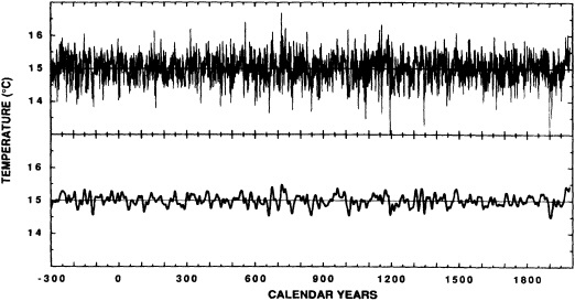
Figure 1
The extended November-to-April temperature reconstruction for Tasmania. The reconstruction covers the period 300 B.C. to A.D. 1989. The period from A.D. 900 is nearly identical to that previously published in Cook et al. (1992). The extension back to 300 B.C. is based on completely independent tree-ring data from old stumps found at the same site. The smooth curve superimposed on the annual values is a smoothing spline that acts as a 25-year low-pass filter.
for the sake of continuity includes a datum for that year.) Qualitatively, the extension prior to A.D. 900 looks similar to, and therefore homogeneous with, the later period. In the next section, we will describe the spectral properties of this record, which indicate the probable existence of interdecadal oscillatory modes in the SH climate system that have persisted over the past 2290 years. Later, we will take a detailed look at these oscillations through time and speculate on mechanisms that might be responsible for their existence.
SPECTRAL ANALYSES
Cook et al. (1992) examined the power spectrum of the Tasmanian temperature reconstruction estimated for the period A.D. 900-1989. Using both Blackman-Tukey and maximum-entropy spectral analysis (Jenkins and Watts, 1968; Marple, 1987), they found evidence for statistically significant (a priori p < 0.05) peaks in the spectrum at approximately 30, 56, 80, and 180 years. Cook et al. (1992) did not examine the properties of these apparent oscillations in the series. However, they speculated that the 30- and 56 year modes could be reflecting similar oscillations in the SH climate system associated with different wave-number flow regimes of the circumpolar zonal westerlies in the 40° to 50°S latitude zone (Enomoto, 1991).
The extended temperature reconstruction described earlier provides us with a rare opportunity to validate the existence of these apparent oscillations. Clearly, if they disappear from the early portion of the extended record, then the physical basis for the existence for these modes is doubtful. For this purpose, we split the series into two essentially independent 1145-year segments covering the intervals from 300 B.C. to A.D. 844 (early period) and A.D. 845 to 1989 (late period).
The Blackman-Tukey power spectra for these periods are shown in Figure 2 (estimates are shown only for periods greater than 10 years). As expected, the late-period spectrum
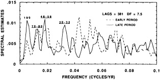
Figure 2
Blackman-Tukey spectra of the first and second halves of the Tasmanian temperature reconstruction. Each half is 1145 years long. The spectra are shown only for periods greater than 10 years. Note the similarity between the spectra in the low-frequency end.
has peaks very close in frequency to those found previously, the principal difference being that the longest-period oscillation is now 190 years. The early-period spectrum likewise has peaks in the same vicinity, although there are some differences. The 190-year peak is more subdued in the earlier period, and the 30-year peak has virtually disappeared. In contrast, the 56- and 80-year peaks found in the late period are present in the early period at closely associated frequencies and with similar power. If the bandwidths of the 56-, 80-, and 190-year peaks in the late-period spectrum are taken into account, the frequencies of the associated peaks in the early-period spectrum are fully covered. The same formal coverage applies for the power estimates in the early period if 80 percent confidence intervals are computed for the late-period peaks. Thus, in terms of both frequency and power, there is little that significantly distinguishes the spectra of the early and late periods at approximately 56, 80, and 190 years. In contrast, the 30-year peak appears to be less stable through time. This result covering the past 2290 years suggests that the putative oscillations are not statistical artifacts.
For completeness, the spectrum of the entire series is shown in Figure 3. The identified periods differ slightly due to the increased record length. All four peaks of interest here exceed the a priori 95 percent confidence level (dashed line), on the basis of a first-order Markov null-continuum model.
SINGULAR SPECTRUM ANALYSIS
The previous spectral analyses revealed the probable existence of oscillatory behavior in warm-season Tasmanian temperatures over the past 2290 years. However, changes in amplitude and phase are indicated, which necessitates a more thorough examination of these oscillations in the time domain. For this purpose we used singular spectrum analysis (SSA), a data-adaptive technique that is particularly well suited for isolating weak signals embedded in red noise (Vautard and Ghil, 1989). SSA decomposes a time series into signal and noise sub-spaces by applying principle components analysis (PCA) to the autocorrelation function (ACF) of that process. Vautard and Ghil (1989) refer to the eigenvectors produced by PCA as empirical orthogonal functions (EOFs) and the eigenvalues as singular values, hence SSA. A pure oscillation embedded in red noise, whose average period is shorter than the length of the ACF, will be composed of an even-and-odd EOF pair. The EOF pair will resemble the shape of the oscillation and be in quadrature (i.e., 90° out of phase). The EOF loadings can be thought of as digital filter weights that are used to estimate the waveform. For this purpose, only the even (or symmetric) EOF, which preserves phase, is used here. Vautard and Ghil (1989) refer to these recovered waveforms as principal components (PCs). The final step of SSA is spectral analysis
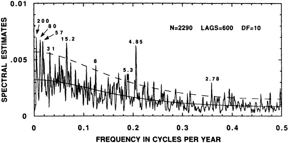
Figure 3
The Blackman-Tukey spectrum of the entire temperature reconstruction shown in Figure 1. A first-order Markov null spectrum was used for constructing the a priori 95 percent confidence level (dashed line). The four spectral periods of interest here are all statistically significant on the basis of these confidence levels, with the 31-year term being the weakest. These results are consistent with the split spectra shown in Figure 2.
of the PCs using high-resolution, maximum-entropy spectral analysis (Marple, 1987).
As in classical spectral analysis based on the Blackman-Tukey approach (Jenkins and Watts, 1968), the number of lags used in computing the ACF for SSA is somewhat arbitrary, being a tradeoff between resolution and stability. Initial experiments indicated that about 300 lags (13.1 percent of the series length) was the minimum needed to simultaneously resolve the 31-, 56-, 80-, and 200-year oscillations. In fact, for lag windows over the range 300 to 700, these four oscillations were always found in the four leading EOF pairs after suitable low-pass prefiltering to remove unwanted high-frequency variance. However, spectral analyses of their PCs indicated that about 400 lags ( 17.5 percent) were needed to cleanly separate the closely spaced 56- and 80-year oscillations. When only 300 lags were used, the spectra of these oscillations were somewhat contaminated by each other's power. In contrast, the 31-year term alone could be reasonably well resolved using only 100 lags (4.3 percent). For this reason, 100 lags were chosen to isolate the 31-year term, while 400 lags were used to isolate the longer oscillations.
Figure 4 shows the four even EOFs estimated as described above. The average period of each EOF is very similar to that obtained from the spectral analysis of its respective waveform. The EOFs are remarkably regular, given that they are based solely on the data and are not constrained to be sinusoidal. Figure 5 shows the normalized power spectra estimated by the maximum entropy method, which confirms the strongly periodic nature of these oscillations. These spectra are purely descriptive and cannot be
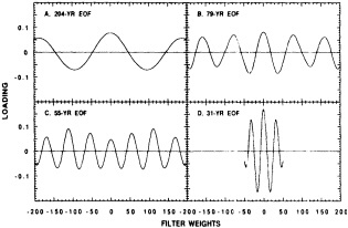
Figure 4
The four even empirical orthogonal functions (EOFs) estimated by singular spectrum analysis representing the oscillatory modes in the temperature reconstruction.
readily tested for statistical significance The identified periods are very close to those found earlier (compare Figures 2 and 3 and Cook et al., 1992). Each spectrum has some degree of side-lobe power in the form of small secondary peaks, which may reflect a degree of amplitude and phase modulation in the waveform. However, they are small enough to be relegated to noise at this stage of analysis. The 31-year oscillation has the most complicated spectrum, with distinct secondary peaks of 29 and 35 years. This may reflect some drift or instability in the mean period over time.
The waveforms upon which the maximum entropy spectra are based are shown in Figure 6. The 204-year waveform
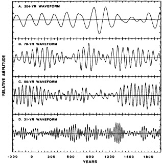
Figure 5
The spectra, estimated by maximum entropy, of the temperature waveforms shown in Figure 6. The spectra have all been scaled to unit peak heights, and the principal peaks are labeled.
is perhaps the most well behaved, with remarkable stability over the first half of the record. However, an increase in amplitude is indicated in the A.D. 900-1200 interval (during the Medieval Warm Period), followed by greatly reduced amplitude in the A.D. 1300-1800 period (during the Little Ice Age). Since about 1800, the 204-year waveform has increased in amplitude to a level not seen since A.D. 1300. The other waveforms are much more complicated, with each showing varying degrees of amplitude and phase modulation.
POSSIBLE LINKS TO THE CLIMATE SYSTEM AFFECTING TASMANIA
The statistical evidence for persistent decade-to-century-scale oscillations in warm-season Tasmanian temperatures is provocative and begs for a physical explanation. We do not have one yet, but some relationships between sea level pressures, sea surface temperatures, and land air temperatures over Tasmania for the past 100 years may provide some clues for where to look.
As noted earlier, Cook et al. (1992) suggested that the 31- and 55-year oscillations could be related to 20-to-30 and 40-to-60 year fluctuations in zonally averaged July sea level pressure (SLP) data in the 40° to 50°S latitude zone (Enomoto, 1991). Specifically, the 20-to-30-year SLP fluctuation was considered by Enomoto (1991) to be a standing oscillation of wave-number-zero structure related to the expansion and contraction of the circumpolar vortex. Inter
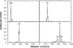
Figure 6
The waveforms of the temperature oscillations identified previously through standard spectral analysis. The waveforms were estimated using singular spectrum analysis, and their units are dimensionless.
estingly, one of the centers of maximum variance was located in the Tasman Sea region ( 130°E to 170°W). The 40-to-60-year fluctuation was considered by Enomoto (1991) to be an oscillation with wave-number-one structure, meaning an eccentricity of the circumpolar vortex. Each of these SLP fluctuations showed large amplitude changes in the 1880 to 1920 interval in the Tasmania-New Zealand sector, with anomalously low pressure being indicated for the 1890 to 1905 period. This implies an expansion of the circumpolar vortex at that time, with a greater tendency for cool, southwesterly winds and below-average temperatures over Tasmania.
A comparison of Hobart SLP data and Tasmanian actual and reconstructed temperatures for the November-to-April warm season supports this interpretation. Figure 7 shows the
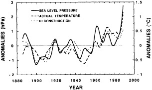
Figure 7
The relationship between warm-season sea level pressure (SLP) at Hobart and temperatures over Tasmania. The cold early-1900s period was characterized by anomalously low SLP. which suggests an expansion of the circumpolar vortex at that time. In contrast, the warm interval beginning in the 1960s was characterized by anomalously high SLP and an inferred expansion of the subtropical high off eastern Australia.
pressure and temperature anomalies since 1886, smoothed to highlight decadal-scale fluctuations. Each series shows persistently negative anomalies in the 1895 to 1920 period, indicating a clear link between anomalously low warm-season SLP and below-average temperatures over Tasmania, presumably related to an expansion of the circumpolar vortex at that time and the northward migration of the subtropical high-pressure belt off the eastern coast of Australia. Figure 7 also indicates a link between SLP and the recent warming in Tasmania. Since about 1960, both warm-season SLP and temperature have been anomalously high, which suggests a southward movement of the subtropical high-pressure belt and a greater frequency of warm, northeasterly winds over Tasmania. This inference is supported by Lough (1991), who showed that the high-pressure belt moved southward about 2° over the 1942-to-1981 period. It is also supported by Coughlan (1979), who showed that annual mean maximum temperatures over Tasmania were significantly correlated with the latitude of the subtropical high.
There is also a possible link between ocean circulation features in the Tasman Sea region and changing land and air temperatures over Tasmania. This link is suggested by changes in the correlation fields of warm-season (November to April) land and marine temperatures versus reconstructed Tasmanian temperatures for two 40-year periods (1888 to 1927 and 1950 to 1989) containing the cold and warm periods indicated in Figure 7. To generate the correlation fields, we obtained corrected land and marine monthly temperature data for 5° × 5° grid cells covering the southern Australia-Tasmania-New Zealand sector. These data were kindly provided by P.D. Jones and K.R. Briffa of the Climatic Research Unit, University of East Anglia, Norwich.
Figure 8 shows these correlation fields. The integer in each cell reflects the correlation coefficient rounded to the nearest tenth. For the cool early period (1888 to 1927), the correlation field is weighted toward the grid boxes off the west coast of Tasmania. This result implies that the inferred expansion of the circumpolar vortex coupled with increased southwesterly winds in the 1890 to 1920 period may have caused the cold West Wind Drift to be displaced northward from its normal position, resulting in anomalously cool temperatures over Tasmania (see Figure 7). In contrast, the correlation field of the late period (1950-1989) is strongly weighted toward the Tasman Sea east of Tasmania. Given the anomalously warm temperatures in Tasmania at that time (Figure 7), this result suggests concomitant warming in the Tasman Sea and more southerly penetration of the warm East Australian Current. In fact, the actual SSTs during this time were anomalously warm, in parallel with warm temperatures over Tasmania. This result is consistent with the southward shift of the subtropical high-pressure belt (Lough, 1991) and increased frequency of warm northeasterly winds over Tasmania.
None of the empirical relationships between Tasmanian
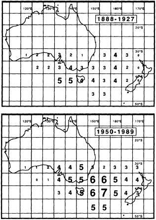
Figure 8
Correlation fields of 5° × 5° grid-cell temperatures versus Tasmanian temperatures for two contrasting cold and warm periods. Each integer reflects a correlation coefficient rounded to the nearest tenth. The 1888-to-1927 period contains the coldest period in the Tasmanian instrumental records, while the 1950-to-1989 period contains the warmest period. Note that the correlation field is weighted toward the western ocean cells during the cold period. During the later warm period, the field is strongly weighted toward the east in the Tasman Sea. The differences in these fields suggest changes in atmospheric and oceanic circulation during cold and warm phases of climate in Tasmania.
temperatures and large-scale atmosphere/ocean processes can explain why oscillations (which have apparently persisted over the past 2290 years) are present in the reconstruction. However, should a physical model be developed, it will probably involve interactions in the atmosphere/ocean/ cryosphere system that influence the movements of the circumpolar vortex and subtropical high-pressure belt. Recently, Stocker and Mysak (1992) proposed that selfsustained oscillations, of similar order to those found here and in many other proxy climatic records. could be induced by internal changes of the ocean thermohaline circulation. Using a simple two-dimensional ocean model, they showed that internal nonlinear dynamics alone could produce self-
sustained oscillations in ocean-to-atmosphere heat flux with periods of 19, 38, and 110 years for the Atlantic Ocean and 110 years for the Pacific Ocean. Similar results have been obtained from a GFDL coupled ocean-atmosphere model (Delworth et al., 1993). Figure 9 shows the power spectrum of detrended mean annual surface air temperatures for the Southern Hemisphere generated by the GFDL model (Delworth et al., 1993). There is a statistically significant (a priori p < 0.05) oscillation in simulated temperatures with a mean period of about 110 years, along with minor secondary peaks at about 56 and 29 years. Thus, there appears to be a reasonable model-based argument for the Tasmanian temperature oscillations' having an internal origin in the Southern Hemisphere ocean-atmosphere system.
With regard to possible solar forcing, we compared our 79- and 204-year waveforms with those related to the 80-to-90-year Gleissberg sunspot cycle and an approximately 200-year oscillation found in high-precision radiocarbon measurements from tree rings (Sonett, 1984; Stuiver and Braziunas, 1989), which Sonett and Suess (1984) have suggested could influence temperatures. These comparisons produced suggestive but equivocal results.
Figure 10 shows the waveform of the 79-year temperature oscillation and the envelope of the annual Wolf sunspot numbers (i.e., the Gleissberg cycle) estimated by SSA for the common period 1700 to 1987. There is a surprising degree of agreement between the two, with temperatures lagging sunspots by about 25 years over the central portion of the curves. However, the phasing apparently breaks down after 1900, with temperatures lagging sunspots by only 10 years. The phase drift may simply mean that the good relationship in the central portion is spurious. However, if sunspot cycle length is used instead of sunspot number as an index of solar activity (Friis-Christensen and Lassen, 1991), the phasing between that index and Tasmanian temperatures actually improves. Peaks in solar cycle length
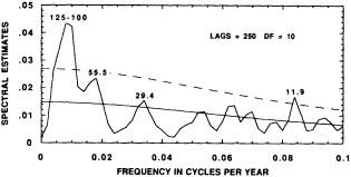
Figure 9
The power spectrum of Southern Hemisphere surface air temperatures generated by a GFDL coupled ocean-atmosphere model. The model was run for 1000 years. A first-order Markov null spectrum was used for constructing the a priori 95 percent confidence level (dashed line). An oscillation with a mean period of around 110 years is clearly indicated in the spectrum.
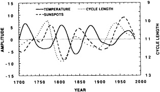
Figure 10
The waveform of the 79-year temperature oscillation compared to the envelopes of sunspot number (the Gleissberg cycle) and sunspot cycle length since 1700. The temperature and sunspot number waveforms were estimated using SSA, and are in dimensionless units. The cycle-length envelope is in years. There is an apparent lag of about 30 to 40 years between Gleissberg-cycle phase and temperature oscillations in Tasmania.
occurred around 1770, 1840, and 1940 (Friis-Christensen and Lassen, 1991). The corresponding peaks in the 79-year temperature waveform occurred around 1805, 1880, and 1970. In turn, solar-cycle-length minima occurred around 1805 and 1900, whereas temperature minima are found around 1840 and 1930. Thus, there appears to be a reasonably consistent lag relationship of 30 to 40 years between Tasmanian warm-season temperatures and solar cycle length since the early 1700s. In being nearly 180° out of phase, this putative relationship either implies that (1) the direct correlation between solar cycle length and Northern Hemisphere temperatures found by Friis-Christensen and Lassen (1991) is effectively opposite in the SH sector around Tasmania, (2) the thermal inertia of the SH oceans significantly delays the response of SH surface air temperatures to solar forcing, or (3) the results of Friis-Christensen and Lassen (1991) and those presented here are spurious. With only about three realizations of the solar-cycle-length envelope available from the sunspot record, it is difficult to make a strong case for either of the first two possibilities.
To compare our 204-year temperature oscillation with the approximately 200-year term in Δ14C, we obtained high-precision decadal radiocarbon measurements of dendro-chronologically dated wood from Stuiver and Becker (1986) covering the period 2500 B.C. to A.D. 1950. These measurements were detrended with a fifth-order polynomial to remove the geomagnetic dipole effect, and the data after 1885 were deleted to eliminate the industrial "Suess effect." Figure 11 shows the residuals from the polynomial curve since 300 B.C., which have also been smoothed to emphasize the century-scale fluctuations in Δ14C. Notable persistent departures are indicated in the A.D. 1100 to 1220 period (the Medieval Solar Maximum) and the A.D. 1450 to 1550 and 1650 to 1700 periods (the Spörer and Maunder Minima,
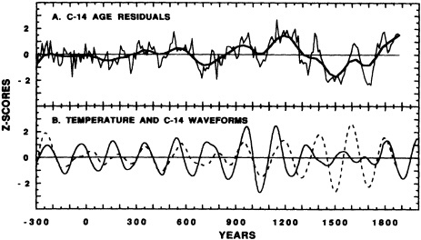
Figure 11
The 14C age residuals from the polynomial trendline (A) and the approximately 200-year waveforms of temperature (solid curve) and 14C residuals (dashed curve) (B). The residuals have also been smoothed to highlight long-term 14C fluctuations particularly evident in the Medieval Warm Period and Little Ice Age. The waveforms are approximately in phase up to about A.D. 1050, after which the relationship breaks down until 1800.
respectively). Prior to A.D. 600, the series is very stable, with few significant long-term departures.
We applied SSA to the Δ14C residuals to isolate the waveform of the approximately 200-year oscillation. This waveform is also shown in Figure 11, with the 204-year temperature waveform superimposed on it for comparison. Not surprisingly, this comparison produced mixed results. There is some degree of phase-locking during the first 1300 years, especially considering the error in the radiocarbon dates of about ± 10 years (Stuiver and Becker, 1986), after which it completely breaks down during the Little Ice Age period until about A.D. 1800. There is also a lack of agreement in the amplitude modulation apparent in each series. The Δ14C oscillation has maximum amplitude through the period of the Spörer and Maunder Minima (also the Little Ice Age). In contrast, the temperature oscillation has maximum amplitude around the Medieval Solar Maximum (also the Medieval Warm Period).
The net result of this examination for a climate-sun link in Tasmanian temperatures at periods of about 80 and 200 years is mixed. If the relationship between solar cycle length and temperatures found by Friis-Christensen and Lassen (1991) is real, then there is some support for a climate-sun link in the temperature reconstruction at a period of 80 to 90 years. The link between the 204-year temperature oscillation and solar variability is more tenuous because of unstable phasing and the mismatch in amplitude modulation noted above. Given these somewhat contradictory results, the climate-sun link cannot be accepted at this time.
IMPLICATIONS FOR DETECTING THE GREENHOUSE EFFECT IN THE SOUTHERN HEMISPHERE
The decadal-scale natural oscillations found in warm-season Tasmanian temperatures indicate that the climate system in this part of the SH is to some degree internally, and perhaps also externally, forced. The level of forcing due to the four oscillations (as a percentage of the total yearly variance in temperatures) is comparatively small, amounting to only about 10 percent. However, when compared to the variance in the reconstruction due to decadal-scale temperature fluctuations alone (i.e., only variance at wavelengths >10 years), the oscillations account for approximately 46 percent of that low-frequency fraction. Given that only four oscillatory modes are necessary to explain a substantial fraction of the low-frequency variance, the following question is posed: To what extent have these natural oscillations contributed to the recent decadal-scale anomalous warming over Tasmania, as described in Cook et al. (1991)?
An examination of the waveform plots in Figure 6 suggests that their collective effect on Tasmanian temperatures since 1960 has been significant. Since that time, all four waveforms have either peaked or are still increasing. In terms of relative amplitude, the 204-year oscillation is also in its most active phase since the Medieval Warm Period. Therefore, it is plausible that the anomalous warming since 1960 in Tasmania is simply due to an unusual coincidence between the four oscillations and an increase in the amplitude of the 204-year term. It is also noteworthy that during
the anomalously cold early 1900s, all of the oscillations were either decreasing or were at a minimum. These relationships are shown in Figure 12, where the four-waveform average is plotted with low-pass filtered actual and reconstructed warm-season temperatures since 1886. The similarity of the curves indicates that both unusually cool and unusually warm decadal-scale temperature anomalies over Tasmania during the twentieth century have been driven in part by long-term climatic oscillations.
This conclusion does not necessarily eliminate greenhouse warming as a possible contributor to the recent tem
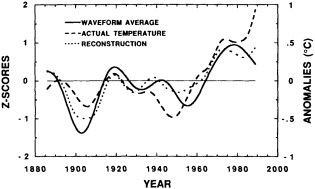
Figure 12
Comparison of the four-oscillation waveform average with actual and reconstructed Tasmanian temperatures for the period 1886 to 1989. The waveform average is expressed in standard normal deviates, while the temperatures are expressed as anomalies. The temperatures have been low-pass filtered to a level comparable to the waveform average. Note the coincidence between the waveform minimum around 1905 and cold temperatures, and between the waveform maximum around 1975 and warm temperatures.
perature increase in Tasmania. Indeed, temperatures since 1985 appear to have increased sharply even as the waveform average has decreased. However, it would be premature to claim that this departure is a manifestation of the greenhouse effect. The average waveform shown in Figure 12 can be used only qualitatively at this time; it does not necessarily contain all of the important terms related to multi-year temperature fluctuations. Nonetheless, its agreement with instrumental temperature data indicates that oscillatory modes with time constants of decades to centuries are an important part of the SH climate system. Until this behavior is better understood, the existence of greenhouse warming in the SH will be difficult to prove.
ACKNOWLEDGMENTS
We gratefully acknowledge the assistance of Trevor Bird (Tasmanian Trades and Labor Council, Forestry Unit) and Mike Peterson (Tasmanian Forestry Commission), who truly made this research possible. In addition, Roger Francey (C.S.I.R.O. Division of Atmospheric Research) and Mike Barbetti (University of Sydney) actively assisted us in our field work. We also thank the Tasmanian Forestry Commission and the C.S.I.R.O. Division of Forest Research in Hobart for local logistical support. Peter Kelly dated and measured the Huon pine stump wood, Rob Allan (C.S.I.R.O. Division of Atmospheric Research) provided the Hobart SLP data, and Tom Delworth at GFDL provided the model-generated SH temperature data. This research is supported by the National Science Foundation, Division of Earth Sciences, Geologic Record of Global Change Program, Grant EAR 91-04922. Lamont-Doherty Earth Observatory Contribution No. 5215.
Commentary on the Paper of Cook et al.
WILLIAM E. REIFSNYDER
I should probably begin with the disclaimer that I am a forester, and by no means a statistician and number-cruncher in the sense that tree-ring people have become. But I strongly believe that one of our best sources of proxy data for the fairly recent past—several thousands of years—is tree-ring chronology. I am delighted to see people working hard and getting good sequences, and I really commend Ed Cook, Brendan Buckley, and Rosanne D'Arrigo for doing just that.
I always get nervous, however, at seeing these power spectra that have peaks with rather little power in them. And I notice too that often when one gets more data many of the relationships either diminish or disappear. I wonder, then, whether this very real problem might be solved with other, quite different data sets. For example, Pieter Grootes told us about the ability of the ice-core analyzers to get very high resolution, on the order of single years, in data from good locations. So to open the discussion, I would like to throw this question out to all of you: Has anyone really attempted to use other data sets to see whether the same peaks will occur in those data?
Discussion
BUCKLEY: We hope to extend our 14C chronology further, which may give us an answer to that question. Also, I expect to find similar temperature resolution at other sites in Tasmania next year.
GHIL: I can show the same peaks from an instrumental record [see Figure 1 in the essay introducing Atmospheric Modeling in Chapter 2]. On a power spectrum of a 300-year record of central England temperatures obtained by the singular spectrum analysis method you can clearly see two interdecadal and two interannual peaks. One is 25, near enough to your 30, and one 14.2, like your 15. The interannual peaks are 7.6, near your 8, and 5.2, matching your 5.2.
MYSAK: The 200-year time scale you passed over rather lightly seems to be the overturning time scale, at least for the Atlantic, and is what we found in our two-dimensional model.
JONES: Michael, it seems to me that your central England temperature record may show the Little Ice Age, but not the modern minimum. A sunspot feature, perhaps. And Brendan, relative to your Figure 10 with the solar cycle length, I wanted to point out that for that Southern Hemisphere pressure data set you're using there are absolutely no data in the zone between 40° and 50° south. Now, the dotted solar-cycle-length curve shows an enormous cycle about 1750 that Kristen and Lassen have postulated as forcing global temperatures. However, they used that curve from 1850 on while ignoring the record back to 1700.
RASMUSSON: These points are awfully important in critically examining what we really have here. But my question is about the treatment of the tree-ring data. Did you have to remove the growth trend, and if so, how did it affect the low-frequency variations?
JONES: The Tasmanian trees are so much longer-lived than the Scandinavian ones I was referring to that it's less of a problem to remove the growth trend.
BUCKLEY: Our paper does talk about bias, particularly at the end of the series, and describes Ed Cook's technique for dealing with it, which is different from Phil's. Also, yew and pine tend not to follow the normal exponential growth curve; they can be very slow-growing subcanopy trees for 200 or 300 years. Often we don't even use those 300 years because it's hard to measure that small growth with any accuracy.
KEELING: If I may, I should like to show for comparison the analysis we made at Scripps of the Jones-Quigley temperature record. I'm not forgetting, of course, that one tends to favor spectral analyses that confirm one's own position. But it seems to me that those spectral lines do come quite close to those we find in the temperature record. The 4.85 line is not far from one of the principal lines of the El Niño signal. Then there are some that may or may not correspond with others. But that 15-year line, that I mentioned was so hard to explain as solar, seems to be quite persistent. It's also half of the 31-year peak I mentioned in my presentation, which is a principal tidal line. It's not as striking as the 93-year cycle, but it's significant. In any case, whether it's the 80 and 200 you showed, and whether there is a Gleissberg effect or not, wherever you see evenly spaced patterns you should look to see what the beat frequency is, and whether it might relate to a long-period line too.
KUSHNIR: I think we need to remember that if we do a spectral analysis with such high resolution and are looking at the 95 percent significance level, there's always the chance that 5 percent of the peaks will be above the line.
MCWILLIAMS: Dave Keeling's tides have very clear frequencies. But in general, why are we looking for lines in the climate record? Why should we expect a priori to see periodicities rather than more distributive broad-band behavior'?
GHIL: We like periodicities because they enhance predictability. But within the context of non-linear dynamics, even though what you observe is broad-band, that is a reflection of instabilities in the underlying phenomena you are trying to track. My suspicion is that each of those lines has a story behind it, and I hope that over the next 10 or 20 years we can begin to understand the interactions of the various phenomena.
REIFSNYDER: It's also true that some of those lines might disappear as more data are accumulated, though our need for cycles—circadian, budget—won't.
KAROLY: I didn't want to talk about cycles, but mechanisms. I think the mechanism you identified as associated with the pressure and temperature fluctuations in Tasmania suggests a structural change, possibly associated with the Antarctic current or the large-scale atmospheric circulation, that fits in quite well with the modulation of the strength of the zonal winds and the large-scale atmospheric circulation on interannual time scales. And it may well be a mode of the decadal and longer time scales as well, with a broad-band rather than a specific frequency.
REIFSNYDER: We should perhaps keep in mind that statistical significance does not equate with reality.
Variability of Atlantic Circulation on Sub-Millennial Time Scales
SCOTT J. LEHMAN1
ABSTRACT
New sediment records from the southeastern Norwegian Sea document a series of abrupt changes in poleward flow of warm surface waters during the last deglaciation (15,000-8,000 yr BP), some of which produced shifts in sea surface temperature of more than 5°C in less than 40 years. These findings confirm the timing, magnitude, and rates of circum-Atlantic climate change implied by ice-core data and predicted by numerical models, and support the theory that the intensity of thermohaline overturning controlled air temperatures around and downwind of the northern North Atlantic.
Unlike the deglacial interval, the last 8,000 years or so have been marked by relatively stable climate conditions in the North Atlantic region. However, as pointed out earlier by Broecker (1987), the conditions that conferred stability over this interval are not yet understood; thus, it cannot be assumed that such conditions will persist in the face of the gradual changes already forecast as a response to anthropogenic perturbation of the climate system.
INTRODUCTION
A key question confronting scientists and policy makers is the degree to which the 0.3°C to 0.6°C rise in globally averaged surface air temperatures observed since the mid-1800s (e.g., Jones and Wigley, 1986) can be ascribed to humankind's impact on atmospheric concentrations of CO2 and other trace-gases. Although the direction and magnitude of the observed temperature change is compatible with many model predictions, the extent to which it may be embraced or overprinted by natural climate variations is not yet known. Indeed, the need to document and understand natural climate variations in this context has motivated many of the contributions to this volume. This paper, on the other hand, views the issue of natural climate variation from a different perspective. Here I present evidence from the end of the last glacial period for natural shifts in circulation of the North Atlantic Ocean that produced regional changes in air and sea temperatures of 5 to 10°C in less than 50 years, which are much too large and sudden to be confused with gradual changes of the type seen in the instrumental record. Rather, the point is that comparable ocean-driven changes might be an unforeseen response to gradual anthropogenic forcing
of the ocean-atmosphere system in the future. Such changes are ''unforeseen" because the vast majority of numerical models used to predict the climate response to CO2 forcing treat the oceans as fixed, or restrict their interaction with the atmosphere to the mixed layer. However, ocean currents are crucial in determining global transports of heat and moisture, and the transient response of climate will thus depend critically on the response of the oceanic circulation. Although the importance of simulating such interactions is widely recognized, it is nevertheless hampered by the difficulty of simulating the general circulation of the oceans (i.e., "getting it right for the right reasons") and the extreme computational requirements of coupling three-dimensional models of the ocean and atmosphere.
Citing the geologic evidence for abrupt climate changes in the past, Broecker (1987) has already articulated the concern that there may be "surprises in the greenhouse" that cannot be adequately portrayed, let alone predicted, using existing models. I follow Broecker's lead here, adding new evidence that, as predicted on the basis of terrestrial indications of rapid climate change around the Atlantic region, ocean circulation patterns and sea surface temperatures varied with degree-per-decade rapidity. Understanding and modeling the mechanisms underlying these changes is of high priority. If, on the one hand, the climate response to increasing greenhouse-gas content of the atmosphere is expected to be gradual, then we may choose to pursue a strategy of adaptation. On the other hand, if we cannot rule out the possibility that the mechanisms that provoked the "surprises" seen in the geologic record may once again become active in the future, we may wish to adopt a policy of restraint, while at the same time trying to enhance our capacity for the recognition and detection of the premonitory signs of abrupt circulation and climate change.
THE CASE FOR "SURPRISES"
There is ample evidence from the geologic and instrumental record for changes in patterns of ocean circulation on a variety of time and space scales. These range from global-scale reorganizations of the thermohaline circulation on glacial to interglacial (105-yr to 104-yr) time scales (Boyle and Keigwin, 1987; Duplessy et al., 1988; Broecker and Denton, 1989; Raymo et al., 1990) to quasi-cyclic, interannual changes of regional scale in historical times, such as El Niño events (Cane, 1983). The spectrum of variability also appears to include possibly cyclic phenomena such as oceanic cooling and reduced ventilation associated with the North Atlantic's Great Salinity Anomaly during the 1960s to 1980s (Dickson et al., 1988b; Lazier, 1988; Mysak and Power, 1991). One of the most extreme examples of rapid ocean circulation change seen anywhere has been inferred from the geologic record of the last deglaciation (15,000 to 8,000 radiocarbon yr BP)2 around the North Atlantic, when air temperatures shifted 5°C to 10°C in a few centuries or less. The proxy record of these temperature changes appears to be coherent over a broad region; it includes oxygen isotopic shifts in Greenland ice cores (Dansgaard et al., 1982, 1989), pollen and isotopic shifts in European lake sediments (Iversen, 1973; Siegenthaler et al., 1984; Ammann and Lotter, 1989), and changes in fossil assemblages of coleoptera in the British Isles (Coope, 1977; Atkinson et al., 1987) (Figure 1). Similar-looking changes characterize the Greenland ice-core record between 8,000 and 80,000 years ago; they thus appear to be a characteristic feature of glacial and deglacial climate in the North Atlantic region (Dansgaard et al., 1982).
The extraordinary rate of these changes was revealed by isotope studies of annually layered ice deposited approximately 10,500 to 10,000 yr BP on Greenland, when air temperatures over the ice sheet rose by 7°C in just 50 years (Dansgaard et al., 1989). As there is no known external (e.g., solar or orbital) climate-forcing agent of sufficient potency and frequency to explain the rapid and recurrent temperature changes seen in these records, the question remains: What process(es) drove the observed variations? The most likely answer, according to a variety of authors (e.g., Oeschger et al., 1984; Broecker et al., 1985), is that they were the result of sudden shifts in the strength and, therefore, in the heat-carrying capacity of the ocean's conveyor-belt circulation system—a global-scale overturning marked by sinking of relatively cold and salty water in the northern North Atlantic, generalized upwelling in the Indian and Pacific oceans, and the return of warm salty surface water to the Atlantic around Africa and South America (Gordon, 1986; Broecker, 1991 a).
The impact of heat transport by the conveyor on the climate of the North Atlantic region is clearly evident in the large positive deviation from zonally averaged January air temperatures centered over and downwind of the northern North Atlantic and Nordic seas, as seen in Figure 2 (after Barry and Chorley, 1982). While there is little doubt that the conveyor contributes importantly to the warmth and habitability of the circum-North Atlantic region (especially northwestern Europe and Scandinavia), a key question from the climate-change point of view is whether the conveyor circulation is subject to significant variation. In an attempt to address this issue, the stability of the conveyor has been investigated in a large number of numerical models of ocean circulation, virtually all of which indicate that its operation is threatened by subtle changes in fresh-water balance at the surface near regions of convection in the northern North
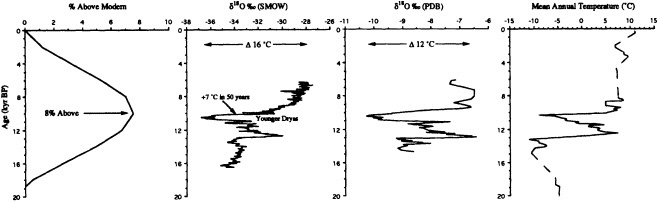
Figure 1
Comparison of insolation and various temperature proxy records for the last deglaciation (0-20 kyr BP). Beginning at the left, they are: the slow change in summer insolation for the Northern Hemisphere during that interval (Berger, 1978); oxygen isotope results from the Greenland ice core Dye 3 (Dansgaard et al., 1984); oxygen isotope results from Lake Gerzensee marls in Switzerland (Siegenthaler et al., 1984); and the mean annual temperature estimate for the British Isles based on fossil coleoptera (Atkinson et al., 1987). Note that summer insolation in the Northern Hemisphere, expressed as a percentage deviation from today's values (first panel), changed gradually over the interval 20 kyr to present. However, various climate proxy indicators from around the North Atlantic region indicate that air temperatures changed abruptly (remaining panels). Detailed studies of Dye 3 by Dansgaard et al. (1989) demonstrate that the large isotope shift at about 10,000 yr BP occurred within 50 years and corresponded to a temperature change of 7°C.
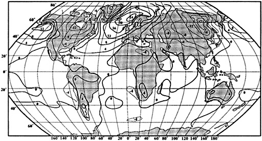
Figure 2
Deviation of local temperatures from the zonal average, for January, in °C. (From Barry and Chorley, 1982; reprinted with permission of Routledge.) The largest positive anomalies overlie the area of conveyor overturning in the northern Atlantic and Norwegian Sea.
Atlantic (see, e.g., Bryan, 1986; Manabe and Stouffer, 1988). In many cases the model circulation is observed to collapse within a few decades of surface freshening (Maier-Reimer and Mikalojewicz, 1989; Stocker and Wright, 1991).
As an example of the possible climate change arising from collapse of the conveyor circulation, Figure 3 shows the depression of (annual) surface ocean and air temperatures associated with the conveyor-off mode in the GFDL coupled atmosphere/ocean general-circulation model (Manabe and Stouffer, 1988). The main point to be made here is that even though the sensitivity of the overturning circulation to fresh-water and temperature forcing at the surface in this (or any other) model cannot yet be validated, cooling of the surface ocean in response to weakened or eliminated conveyor circulation is capable of producing pronounced cooling of the air over and downwind of the North Atlantic. This is further borne out by the results of an earlier experiment in which Rind et al. (1986) used the NASA-GISS atmospheric general-circulation model with sea surface temperatures specified (rather than freely pre-
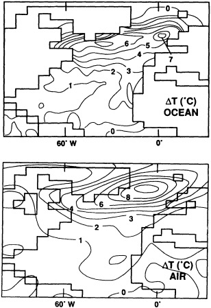
Figure 3
Difference in sea surface and surface air temperatures between the "conveyor on" and "conveyor off" states in the GFDL coupled atmosphere-ocean model (after Manabe and Stouffer, 1988; reprinted with permission of the American Meteorological Society). Although the sensitivity of the conveyor circulation in this model (and others) is debated, and cannot yet be empirically evaluated, there is little doubt that a weakening or elimination of the overturning conveyor circulation will lead to cooler sea and air temperatures in and downwind of the northern North Atlantic region.
dicted) at the cold, wintertime values reconstructed for the last glacial maximum (the LGM, which occurred about 18,000 yr BP) by CLIMAP (1981). As can be seen in Figure 4, a similar pattern of cooling (in this case, wintertime) was achieved. Although the presence of large ice sheets contributed to oceanic cooling during the LGM (Manabe and Broccoli, 1985), in both this and the coupled atmosphere/ocean experiment ice sheets were not introduced, and all other climate boundary conditions were those of today. Figures 3 and 4 provide an impression of the influence of a cold ("conveyor off") ocean alone.
The main purpose of the present paper is to assess the capacity of the ocean to undergo circulation changes of the magnitude and rapidity suggested by the climate proxy
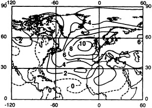
Figure 4
Difference in wintertime surface air temperatures between the control run and one with sea surface temperatures specified at glacial (LGM) values reconstructed by CLIMAP (1981). The results are similar to those seen for air temperatures in the GFDL coupled model (Figure 3, lower panel), although these are for wintertime and the area of maximum temperature difference is located somewhat further south, in accordance with the difference between the location of maximum ocean cooling as reconstructed for the LGM and simulated for the "conveyor off" state in the upper panel of Figure 3.
record around the Atlantic region, through a review of the evidence for such changes in the ocean sediments themselves. Following up on the discussion brought forward in this introduction, I will begin by assessing the magnitude of heat transport into the circum-Atlantic region by the ocean's conveyor circulation system. I will then outline the approach used in reconstructing past changes in conveyor circulation and present results from studies of new Atlantic sediment records with sub-century-scale resolution and climate sensitivity sufficient to capture the amplitude and rates of climate change implied by ice-core studies and numerical models (Lehman and Keigwin, 1992; Koc-Karpuz and Jansen, 1992). These provide a test of the proposed conveyor model of circum-Atlantic climate change, as well as an assessment of the frequency and abruptness with which the conveyor circulation may vary.
HEAT TRANSPORT AND THE ATLANTIC CONVEYOR
The net transports of heat and salt in the world's oceans are characterized by a southward, trans-equatorial flow of relatively cold, salty North Atlantic Deep Water (NADW) formed by cooling and sinking in the northern North Atlantic, and an apparently compensatory, northward, trans-equatorial flow of warm, salty water in the Atlantic thermocline (Gordon, 1986; Broecker, 1991 a). Cooling and sinking occurs predominantly in the Labrador and the Nordic seas (Figure 5). The dense products of surface cooling in the
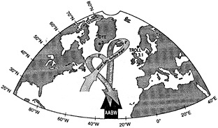
Figure 5
A schematic representation of the components of NADW that can be traced directly to source areas at the surface of the northern North Atlantic. As discussed in the text, these components may comprise as little as two-thirds of the total southward flux of NADW. The remainder may derive from entrainment of recirculated waters. Temperatures (in °C) refer to the surface temperatures just prior to convection, and to the average temperature of each of the convecting water masses that feed upper and lower NADW (cf. Clarke and Gascard, 1983; Aagaard et al., 1985; Bainbridge, 1981).
Labrador Sea descend directly to the interior of the open Atlantic, and are the dominant source of upper NADW (McCartney and Talley, 1984; Clarke and Gascard, 1983). While cooling and sinking occur at a variety of locations within the Nordic seas, the dense waters overflowing the Denmark Strait and crossing the Iceland-Faeroe Ridge into the open Atlantic appear to originate primarily from intermediate-depth convection within the Iceland Sea (Aagaard et al., 1985). These waters, which are denser than those formed in the Labrador Sea, are the dominant source of lower NADW (Worthington, 1976). Together these water masses comprise approximately two-thirds or more of the total southward, trans-equatorial transport of NADW. The remainder may result from entrainment of Antarctic Bottom Water (AABW) and Antarctic Intermediate Water (AAIW) (McCartney and Talley, 1984; Schmitz and McCartney, 1993). The southward-flowing deep waters upwell toward the surface at a variety of locations in the Pacific and Indian oceans. From these locations surface waters are returned to the Atlantic either via the Drake Passage (the "cold-water route") or via the Straits of Indonesia and the Aghullas retroflection around Cape Hope (the "warm-water route"). These return flows complete the Great Ocean Conveyor loop described by Gordon (1986) and Broecker (1991a). Estimates of the net deep-water export from the North Atlantic, based on a variety of different approaches (Broecker, 1991a; Schmitz and McCartney, 1993, and references therein; Wunsch, 1984), range between 14 and 20 sverdrups (1 Sv = 106 m3/sec).
Broecker (1987, 1991b) made a rough calculation of the heat release to the atmosphere resulting from warm-to-cold water conversion by the conveyor, assuming average temperatures of 11°C for northward-flowing thermocline waters and 3°C for southward-flowing NADW. Using an estimated flux of NADW of 20 Sv, approximately 5 × 10²¹ calories are released to the northern atmosphere per year (i.e., about 0.7 petawatt). According to the circulation scheme of Schmitz and McCartney (1993), however, as much as 5 to 7 Sv of the total southward flow at depth is comprised of relatively old, cold, recirculated deep waters that have not been directly involved in warm-to-cold water conversion at the surface of the northern North Atlantic. Using this transport scheme, which also depicts a larger proportion of the compensatory northward flow at greater, colder depths, the average temperature of surface and near-surface waters subject to warm-to-cold conversion is 8°C, and the flux of NADW produced by convection in the northern North Atlantic is only 13 Sv, yielding an estimated heat release of about 2 × 10 21 calories per year.
The two different estimates can probably be regarded as extremes that bracket the actual heat release to the atmosphere over the northern North Atlantic. (I suggest this because (1) in these calculations the larger estimate of deepwater flux is tied to the larger estimate of temperature difference between exported deep water and returning surface water, and vice versa, and (2) the smaller estimate of NADW flux would predict a nutrient content for the deep Atlantic at the high end of what can be accommodated by current observational estimates.) In any case, the impact of the conveyor, on the basis of heat release alone, is huge. Broecker (1987, 1991a) noted that his estimate of 5 × 10²¹ calories per year was equivalent to approximately 30 percent of the solar energy absorbed by the troposphere over the northern North Atlantic. The fingerprint of this oceanic heat source is seen in Figure 2. Its removal would result in temperature deficits similar to those seen in Figures 3 and 4. It follows from these examples that changes in the strength of the conveyor may exert a strong influence on the climate of the North Atlantic region.
THE PROXY RECORD OF SURFACE CIRCULATION
The proxies used here to assess past variations in the strength of the conveyor circulation are changes in fossil assemblages of planktonic foraminifera (carbonate-shelled protozoans) and diatoms (silica-shelled plants) with known temperature tolerances. Fossil assemblages of planktonic foraminifera, in particular, have been used routinely to chart the history of polar-front movements and related rates of surface-circulation change in the North Atlantic (McIntyre et al., 1976; Ruddiman et al., 1977; Ruddiman and McIntyre, 1981; Bard et al., 1987). The general premise is that northward penetrations of subtropical to subpolar assemblages occurred during periods when poleward flow of Atlantic surface waters was vigorous (as it is today), and that south-
ward penetrations of polar assemblages occurred during periods of reduced poleward surface flow, such as the LGM (see, e.g., McIntyre et al., 1976; Kellogg, 1980). These states can be equated with what Broecker and colleagues have termed "conveyor on" and "conveyor off" modes, and with meridional versus zonal orientations of the North Atlantic polar front, respectively (see Figure 6, for example).
Synoptic reconstructions based on studies of a large number of Atlantic deep-sea sediment cores have outlined the general pattern of polar-front movement during the last deglaciation (Ruddiman and McIntyre, 1981). The front began to retreat from its LGM position approximately 13,000 yr BP, then advanced southward once again between about 11,000 and 10,000 yr BP during the well-known Younger Dryas cold interval, just prior to a final retreat to near its present position (see Figure 6). Initial attempts to calculate the rate of polar-front migration during the deglaci
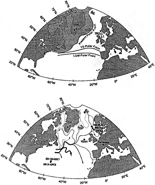
Figure 6
Above, map of the present, LGM, and Younger Dryas polar fronts and the approximate range of polar foraminifera today (after Ruddiman and McIntyre, 1981; printed with permission of Elsevier). Below, a schematic of the main surface transports in the northern North Atlantic (after Dietrich et al., 1975; reprinted with permission of John Wiley & Sons and Gebüder Borntraeger). Solid lines in the latter refer to warm-water transport and dashed lines to cold-water transport. Line thicknesses are roughly proportional to flux. The surface flux of warm waters toward areas of warm-to-cold conversion in the Labrador and Nordic seas is estimated to be that required to balance the export of new NADW production (see Figure 5).
ation suggest that, in the fastest case, it swept between extreme positions in less than 400 years (Bard et al., 1987). This estimate is close to the maximum rate that can be discerned using 14C dates from different sediment cores. The typical precision of 14C ages between 8,000 and 15,000 years BP is ± 80 to ± 160 years at 1s; the compound error associated with dating isochronous events in two different cores is therefore ± 160 to ± 320 at the 80 percent confidence level (1 s), and twice that at the 95 percent confidence level (2s). Although the individual (and therefore compound) errors can be reduced by dating the same stratigraphic level repeatedly, even if there were no other stratigraphic uncertainties such as bioturbation (stirring by bottom-dwelling organisms), approximately 100 such dates would be required to reduce the error from several centuries to several decades (using 2s/n1/2). It is therefore not surprising that such estimates of circulation response time greatly exceed those suggested by ice-core studies.
Rather than fight the errors involved in trying to chart the sweep rate of faunal boundaries between cores, one can alternatively measure the timing and rates of faunal change at a single site that is diagnostic of the overall behavior of the Atlantic circulation system. One such location is the region between the Faeroe Islands and southwestern Norway, which is effectively a gateway to the Nordic seas through which warm surface waters are drawn by deepwater formation and export across the Iceland-Faeroe Ridge and through the Denmark Strait. At this location, the degree and rate of warming or cooling indicated by faunal changes should be indicative of both the degree and the rate of change of poleward surface-water flow through the northern North Atlantic. Because conditions in the Norwegian Sea would be of uniformly polar character in the absence of Atlantic inflow, it is sufficient for the present purpose to measure the proportion of the single polar taxon, Neogloboquadrina pachyderma (sin), with respect to the sum of all planktonic foraminifera. N. pachyderma (sin) constitute more than 95 percent of the fauna at summer sea surface temperatures (SSTs) below 5°C or so (polar and Arctic water masses) and are extremely rare in waters with summer SSTs above about 10°C (Bé and Tolderlund, 1971; see Figure 7). Summer temperatures in this range are associated primarily with the region of mixing between Atlantic and polar waters within the basin today (Johannesson, 1986; Lee and Ramster, 1981). Past changes in N. pachyderma (sin) percentages between values corresponding to the 5°C and 10°C isotherms should record nearly the full range of SSTs associated with past changes in flow of Atlantic waters into the basin.
Measurements of N. pachyderma (sin) percentages were carried out in core Troll 3.1 from an area of high deposition rates in the western North Sea (see Figure 6b for core location). The seismostratigraphy, lithostratigraphy, and dating of the core site are described in Lehman et al. (1991).
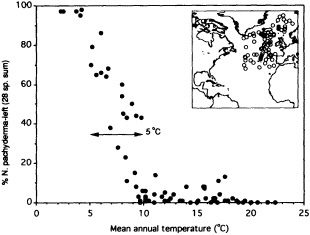
Figure 7
Percentage of N. pachyderma (sin) in core-top sediments from the northern North Atlantic and Norwegian Sea versus temperature of the overlying surface waters. N. pachyderma (sin) percentage appears to have a range of temperature sensitivity of about 5°C. The inset map shows the location of the sediment cores used in the calibration. Data used in this figure were supplied by David Anderson of the National Geophysical Data Center, NOAA.
Average rates of deposition at the core location were 5 m/kyr during deglaciation, some 20 to 50 times higher than at other high-deposition-rate locations in the open Atlantic. The core site is located a few degrees east of the main axis of Atlantic water inflow to the Norwegian Sea basin (Figure 6b). Atlantic water bleeding off the main axis of inflow and into the North Sea greatly influences SST and salinity over the core site, as is clearly apparent in satellite images of the region (see Figure 8, in the color well). Instrumental data suggest that changes in salinity and SST of the North Sea reflect similar changes in the open North Atlantic (Dickson et al., 1984; Heath et al., 1991). These observations suggest that the location Troll 3.1 provides a suitable monitor of surface water exchange between the open North Atlantic and the Nordic Seas.
The down-core variation in percentage of N. pachyderma (sin) and associated accelerator mass spectrometer (AMS) 14C dates in Troll 3.1 are given in Figure 9. These match closely the faunal variations from another AMS 14C-dated sediment core located off Ireland (core V23-81), just upstream of Troll 3.1 in the present-day circulation (Figure 6b; Ruddiman et al., 1977; Broecker et al., 1988). The agreement between these records provides additional evidence that faunal changes in the western North Sea were diagnostic of conditions in the open Atlantic during the last deglaciation. While the two records are complementary in this regard, the record in Troll 3.1 offers a key advantage in that rates of deposition are high enough to permit resolu-
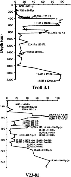
Figure 9
Percentage of N. pachyderma (sin) against depth. The panel for core Troll 3.1 includes AMS 14C dates from Lehman et al. (1991). Despite the large difference in depth scales, the downcore pattern is similar to that in core V23-81 panel, which is from Ruddiman et al. (1977, reprinted with permission of the Royal Society) and includes dates from Broecker et al. (1988, 1990b). The largest N. pachyderma (sin) peak in each core occurred during the Younger Dryas. Although dates of the N. pachyderma (sin) peak just prior to the Younger Dryas in V23-81 are discordant with those for a similar event in Troll 3.1, bracketing dates on subpolar foraminifera (Globoratalia bulloides) are similar. Detailed analyses of photographs of V23-81 indicate that out-of-sequence dates come from worm burrows (G. Bond, personal communication). Arrows mark faunal transitions in Troll 3.1 corresponding to SST changes of about 5°C in 40 years or less. (From Lehman and Keigwin, 1992; reprinted with permission of MacMillan Magazines.)
tion of the true rates of faunal change at the site, unmasked by bioturbation.3
The comparison of high-resolution faunal results for Troll 3.1 with other climate proxy records leads to the following conclusions concerning the variability and climatic impact of surface circulation during deglaciation:
-
In addition to initial deglacial warming from approximately 13,500 to 13,100 yr BP (20 to 18 m depth in core) and the Younger Dryas cold oscillation between about 11,200 and 10,500 yr BP (6 to 4 m), both of which have been recognized and dated previously in several cores from the northern North Atlantic, additional warm-cold-warm oscillations are documented at about 12,600 to 12,400 yr BP (15 to 10 m), 11,700 to 11,500 yr BP (8.5 to 7 m), and 9,700 yr BP (3.8 m) (see Figure 9). Although none of these oscillations was as severe as the Younger Dryas, they indicate that the surface limb of the conveyor was more variable in strength than previously imagined.
-
Estimates of the duration of single warm-to-cold and cold-to-warm transitions based on interpolation between 14C dates indicate that several of these transitions (marked by arrows in Figure 8) occurred in 40 years or less. As these transitions span the full or nearly the full range of conditions recorded by N. pachyderma (sin), they represent swings between near-present-day levels and near-absence of Atlantic water within the basin, that is, between near-extreme states of the conveyor circulation. These changes appear to occur with an abruptness similar to that of the isotopic shifts recorded in Greenland ice cores (Dansgaard et al., 1989). (The transition to warmer water conditions at the close of the Younger Dryas appears to have taken around 100 years, but since deposition rates at the site of Troll 3.1 drop to about 1 m/kyr by this time, the apparently slower transition may be an artifact of the decrease in stratigraphic resolution. Nonetheless, absolute rates of SST change at this time may have been just as great as earlier ones. As we shall see below, this transition may have involved a warming of as much as 9°C; see, e.g., Figure 10.)
-
On the basis of the observed range of temperature sensitivity of N. pachyderma (sin), Lehman and Keigwin (1992) estimated that larger faunal changes in Troll 3.1 corresponded to changes in SST of 5°C or more. A new, independently dated, high-resolution record of SST changes in the southeastern Norwegian Sea based on diatom assemblages, which have a much broader range of temperature
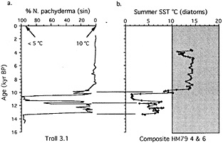
Figure 10
Comparison of N. pachyderma (sin) percentage in Troll 3.1 (panel a) with an estimate of summer SSTs based on diatom assemblages in an independently dated, composite record of two cores (HM79 6/4, panel b) from the southeastern Norwegian Sea (see Figure 6b for core locations). The diatom record is from Koc-Karpuz and Jansen (1992). The area of shading marks SSTs outside the ecological range of N. pachyderma sin) indicated by data in Figure 7 and by Bé et al. (1971).
-
sensitivity than N. pachyderma (sin), confirms the earlier estimates from Troll 3.1 (Koc-Karpuz and Jansen, 1992). The comparison in Figure 10 shows that the range of SST that might be inferred from the percentage of N. pachyderma (sin) was truncated primarily at the warm end, as might be expected on the basis of present knowledge of its modern distribution (e.g., Bé and Tolderlund, 1971). The duration of major SST changes evident in Troll 3.1 and the magnitude of change confirmed by the diatom record suggest that the rates of SST change in the southeastern Norwegian Sea were approximately 1°C per decade, which is directly comparable to the rates of air-temperature change inferred from ice-core studies.
-
When plotted by age, the percentages of N. pachyderma (sin) variations in Troll 3.1 correspond closely with the history of mean annual air temperatures over the Greenland ice sheet deduced from changes in d18O of ice in Dye 3, which has the highest resolution of the long Greenland ice cores (Figure 11). This relationship is consistent with earlier suggestions that sudden changes in circum-Atlantic temperatures were governed by changes in strength of the conveyor circulation (Oeschger et al., 1984; Broecker et al., 1985). The strong similarity of temperature proxy records from Greenland, Britain, and Switzerland (Figure 1) indicate that conveyor circulation also affected air temperatures downwind of the northern North Atlantic at least as far as central Europe, in accordance with model predictions (e.g., Rind et al., 1986; see Figure 4).
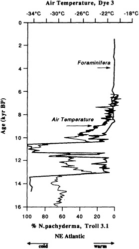
Figure 11
N. pachyderma (sin) percentage in Troll 3.1, plotted to age using the 14C dates in Figure 9, and compared with mean annual air temperature based on d18O of ice from core taken at Dye 3, Greenland. The age-to-depth relationship in Dye 3 is roughly linear prior to approximately 10,000 yr BP, as suggested by correlation to dated variations at Lake Gerzensee. The correlation between Troll 3.1 and Dye 3.1 after about 10,000 yr BP is based on annual layer counting and 14C-to-calendar year conversion, as discussed in Lehman and Keigwin (1992). As a result, the age model after 10,000 yr BP differs slightly from that used in Figure 1b of Hammer et al. (1986).
CONCLUSIONS
A series of abrupt changes in the poleward flow of warm surface waters has been documented in the northeastern North Atlantic during the last deglaciation (15,000 to 8,000 yr BP). They appear to correlate with evidence of atmospheric temperature changes over Greenland and downstream over Europe. Most important, they provide the first direct indication of the capacity of the conveyor circulation to shift abruptly in strength, as recorded by changes in temperature on the order of I C per decade across a range of more than 5°C at the surface of the northern North Atlantic. Numerical models of ocean circulation produce large changes in vertical and lateral ocean-heat fluxes in the North Atlantic as a result of changes in thermohaline circulation arising from fresh-water forcing at the ocean surface (Manabe and Stouffer, 1988; Maier-Reimer and Mikalojewicz, 1989; Stocker and Wright, 1991). Although the sensitivity of the different models to fresh-water forcing is debated and cannot yet be empirically evaluated, the rates and magnitude of the simulated changes now find support from high-resolution proxy records of ocean-circulation change. Owing to associated changes in heat transport, these non-linear aspects of circulation change must be considered a potent agent of climate variability.
Unlike the deglacial interval discussed in this paper, the last 8,000 years have been marked by relatively stable climate conditions in the North Atlantic region (Figure 11). But, as pointed out earlier by Broecker (1987), the conditions that conferred stability over this interval are not yet understood; thus, it cannot be assumed that such conditions will persist in the face of the gradual changes already forecast as a response to anthropogenic perturbation of the climate system.
ACKNOWLEDGMENTS
I wish to thank Delia Oppo and Bill Curry for stimulating discussions and their reviews of an early draft of this manuscript. Julia Cole also provided useful criticism. Ernest Joynt III and Fritz Heidi assisted with graphics. This work was supported by NSF grants OCE-90819660 and OCE-91816259.
Commentary on the Paper of Lehman
JULIA E. COLE
University of Colorado
In commenting on Dr. Lehman's paper, I would like to start by pointing out a few things that he has not emphasized, which make it especially relevant to observational data and model simulations.
Paleoclimate reconstructions play a unique role in the study of ocean-atmosphere dynamics, by offering a window onto climate during periods that we cannot observe firsthand. Dr. Lehman's paper provides strong evidence for rapid (that is, decadal) transitions in oceanic circulation during the last deglaciation, and highlights the information to be found in high-resolution studies of the marine sediment record.
Certain aspects of this study make it particularly complementary to ocean modeling studies. First, the site is sensitive to a specific aspect of the large-scale "conveyor belt" of ocean circulation. The core has extremely high, continuous sedimentation rates for the period of interest, which are critical to addressing rapid climate change. The response of the paleoceanographic proxy to temperature change, including its range of sensitivity, is well characterized in the modern ocean and provides quantitative estimates of SST changes. Chronologic control over this interval is extremely tight, which makes it possible to estimate rates of paleoceanographic changes. The rapid rates of circulation change inferred from the Troll core are in fact consistent with the high degree of sensitivity simulated by ocean GCMs for the ocean circulation conveyor.
This study raises many questions about past and future ocean-circulation dynamics. The Troll core provides a high-resolution window onto only a few thousand years, in the most recent deglaciation. Are rapid changes in the conveyor intensity characteristic of full glacial and interglacial as well as deglacial climates? New ice-core records from Greenland and Antarctica may help to shed light on this question. But high-resolution records from the ocean will be required as well, to help us understand the relationship between changing climate boundary conditions and the linear and nonlinear responses of large-scale ocean circulation.
This study challenges traditional ideas about the speed at which the oceanic conveyor starts and stops, and presents new observations on ocean sensitivity that concur with both ice-core evidence and model behavior. If rapid changes in the Troll core truly represent rapid changes in conveyor circulation intensity, they should be apparent in other North Atlantic records with short response time and high resolution. Such records will test and add detail to the proposed model of deglacial ocean circulation, in which distinct source regions vary in their contributions to northern-source deep water.
The recognition that ocean circulation has changed rapidly, and that we can reconstruct these changes in detail, should intensify efforts to focus paleoceanographic sampling and analysis strategies on decade-to-century-scale objectives. To reconstruct high-frequency oceanic variability, we need to target environments where rapid changes can be preserved by high sedimentation rates (where possible, in annually laminated sequences). We also need to encourage continuing support for appropriate coring techniques, rigorous dating, and proxy calibration. A new emphasis on high-resolution paleoceanography will help us to close the "information gap" that exists between annual and Milankovich time scales of climate variability, and will provide insight into how the climate system responds on societal time scales to changing boundary conditions.
Discussion
RIND: You called the oscillation seen during the last time period "characteristic of the system". It would be interesting to see whether you could find perturbations like this during the last interglacial.
LEHMAN: We intend to do just that at Bermuda Rise. I also think that it might be fruitful to begin to simulate these 3000-year oscillations that appear to arise from some sort of salinity forcing. But these variations during glacials are hard to relate to the kind of variability we seem to see during interglaciation, which may be what the two different limbs of my double conveyor belt reflect. There might be a link between the spatial and temporal variability.
RIND: How do you square the subtropical gyre's apparent sensitivity to thermohaline circulation with the CLIMAP reconstruction of very little temperature change there at a time when we know that the thermohaline circulation was strongly restricted?
LEHMAN: Well, CLIMAP could be wrong. Maybe I should submit a proposal to test their conclusions by doing organic geochemi-
cal analysis. I have great faith in the high-amplitude variability we've found in our high-resolution records from the Bermuda Rise core. We have a very sensitive site and materials with a high deposition rate, and because the subtropical area isn't sensitive to front movement I really think it's diagnostic of a large part of the ocean.
GROOTES: I'd like to show some records of decadal-scale isotope fluctuations in the GISP2 core that complement what Scott has been showing us. Figure 4b in my paper shows these fluctuations for the last few hundred years, but they are even stronger during the glacial-to-interglacial transition about 14,000 years ago. If we use the same isotope-temperature gradient of 0.63 permil per °C, we calculate a change in mean annual temperature of about 10°C over a 5-year period. The electroconductivity of the ice, which reflects neutralization of acidity by alkaline dust, also indicates large and very rapid climate fluctuations—both interstadial Dansgaard-Oeschger events on a time scale of centuries, and periods of very high climate instability on a decadal time scale. We have to ask what caused the rapid changes in air circulation reflected by the dust and temperature changes at GISP2.
COLE: Could they just be a function of change of source regions? Could you use deuterium excess to distinguish source and local climate changes?
GROOTES: Deuterium excess can be used to separate changes in local climate from changes in the source region of the water vapor. Even if the observed changes are a function of a change in source regions, we still need to find a cause for this latter change, one that can effect very rapid changes. We need to put together all our climate data—ice-core, ocean, terrestrial, instrumental—to determine the mechanism for these rapid climate fluctuations. It won't be easy, but we should be able to sort it out eventually.
NORTH: Could those large fluctuations relate to the extremely large ice sheet in North America at that time?
LEHMAN: Such an ice sheet ought to buffer the Pacific/Atlantic isotope source differences. We've got a lot to look at.
Ice Cores as Archives of Decade-to-Century-Scale Climate Variability
PIETER M. GROOTES1
ABSTRACT
Ice cores form a unique archive of past climatic and atmospheric conditions, because they can record these conditions continuously, with annual resolution, and may preserve them over very long times. The information that can be deduced from an ice core includes temperature fluctuations, derived from stable-isotope ratios of hydrogen and oxygen in the ice; chemistry and dust content, reflecting availability in the source area or biospheric activity, as well as atmospheric transport; and volcanic eruptions, recorded as high non-sea-salt sulfate concentrations and sometimes as volcanic ash. The composition of the atmosphere in the past is preserved in air bubbles trapped in the ice, while cosmogenic isotopes reflect the intensity of cosmic rays reaching the earth, and may be useful for dating the core.
The new ice cores from the summit area of the Greenland ice sheet show considerable variability on decadal time scales. Century-scale fluctuations are small during the Holocene, but frequent and large before that. A multiparameter core analysis allows a reconstruction of the changes in atmospheric circulation and in the biosphere (terrestrial and marine) that accompany climate change.
INTRODUCTION
Understanding decade-to-century-scale climate variability requires not only high-resolution climate records for at least the last 1000 years, but also a good definition of the background of slow climate changes on which shorter climate variations are superimposed. The ideal is to have long (>105 yrs), high-resolution records showing the full range of natural climate variability, from glacial/interglacial and stadial/interstadial (on 103 to 105 year time scales) to decadal. In addition to the long-term background of climate change, the long records also offer a better opportunity to ascertain what interactions in the climate system determine climate change, because the major changes in atmospheric circulation and composition and in land and ocean surface conditions that accompany glacial/interglacial climate change are much better defined than the comparatively minor changes of the last several thousand years. Yet the small climate
changes on a decade-to-century time scale are important for society, because these may significantly affect living conditions.
Reliable instrumental observations go back only about a century, so for the study of climate variability we are dependent on proxy records. Many different sources of proxy records have been used, such as ocean and lake sediments, peat bogs, tree rings, speleothems, loess deposits, and ice cores. Problems in the reconstruction of climate from proxy sources are that the climate information recorded depends on the response time and sensitivity of the recording systems, which differ from proxy to proxy, and that recording is often discontinuous and represents merely local conditions. Thus we need to combine records from different sources and areas into a consistent picture to reconstruct global climate variations.
An example of the difference in recording properties of three common climate proxies is given in Figure 1. Climate in northwest Europe during the last glacial-to-interglacial transition, reconstructed from pollen analyses (Figure 1a: Van der Hammen et al., 1967), showed two interstadial periods. The younger one contained the more warmth-loving pollen assemblages, and thus was believed to be the warmer of the two. However, oxygen isotopes in ice cores (Figure 1b: Grootes, unpublished; also Dansgaard et al., 1982, 1984, 1989; Johnsen et al., 1992a) and in lake sediments (Oeschger et al., 1984) as well as beetle remains (Figure 1c: Coope, 1977; Coope and Brophy, 1972; Atkinson et al., 1987) indicate that warmer conditions prevailed during the older interstadial. In this case the pollen represents a distorted climate record (see also Kolstrup, 1990), because climate changed more rapidly than vegetation could respond, and the fluctuations were more faithfully recorded by the faster-reacting isotopes and beetles. Trees, which are frequently used as climate indicators in the arboreal part of the pollen spectrum, migrate particularly slowly into new territory in response to climate change. Reconstruction of decade-to-century-scale climate variations thus requires a fast-reacting climate recorder that preserves a high-resolution environmental record over long time periods. Ice is such a recorder.
ICE CORES AS ENVIRONMENTAL ARCHIVES
High-latitude and high-altitude cold ice masses contain a record of past climate and atmosphere that is unique, because it may be deposited as continuous, discrete annual
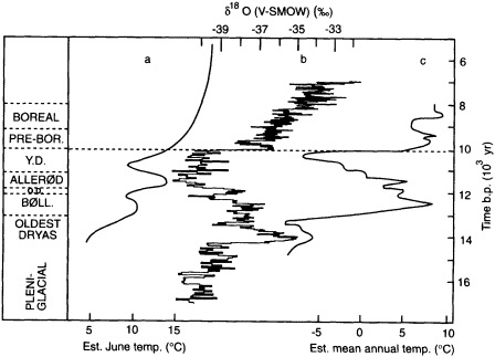
Figure 1
Climate change across the last glacial-to-interglacial transition as reconstructed from (a) northwest European pollen assemblages (after Van der Hammen et al., 1967), (b) the GISP2 oxygen isotope record, and (c) beetle remains in Great Britain (Coope and Brophy, 1972; Coope, 1977; Atkinson et al., 1987; modified from Atkinson et al., printed with permission of Macmillan Magazines Ltd.), each on its own relative time scale. The rapid warming from Younger Dryas to Preboreal has been used to line up the three curves at 10,000 yr before present (Mangerud et al., 1974). The latest results from the GISP2 and GRIP cores and from elsewhere indicate that the Younger Dryas-Preboreal transition really occurred around 1 1,600 years ago (Johnsen et al., 1992a; Alley et al., 1993). The d 18O values for Greenland are generally translated into temperature changes using 0.63 permil per °C (Dansgaard et al., 1973). The slow response of the pollen assemblages to the extremely rapid climate changes during the transition indicated by (b) and (c) led to an underestimate of temperatures in the Bølling, which was therefore considered to have been cooler than the Allerød.
layers of snow, and be preserved with little alteration over long periods of time (>105 years in the central areas of cold ice sheets). Moreover, the ice preserves a direct record of the atmospheric aerosols and gases. Over the past 30 years much research has been done on ice cores and on the climatic and environmental information they contain. Excellent summaries are given in The Climatic Record in Polar Ice Sheets (Robin, 1983) and The Environmental Record in Glaciers and Ice Sheets (Oeschger and Langway, 1989). A review of global ice-core research is outside the scope of this paper, which aims to demonstrate that ice cores can provide detailed records of rapid climate fluctuations going back far in time. To provide access to the ice-core research literature, a limited selection of ice-core references, grouped under water isotopes, chemistry, dust, and gases, appears in Table 1.
TABLE 1 Ice-Core Research References
|
Core |
d18O, dD |
Chemistry |
Dust |
Gases |
|
Greenland |
|
|
|
9,10,11 |
|
Camp Century |
1,2,3,4 |
5,6,7 |
8 |
9,16,17,18,19,20,21 |
|
Dye-3 |
2,12,13,14 |
7,15 |
13 |
|
|
Renland |
22,23 |
22,24 |
22 |
|
|
GRIP/GISP2 |
23,25,26,27,28 |
25,27,29,30,31,32,33 |
|
34,35 |
|
othera |
36,37 |
5,6,30,31,38 |
|
39 |
|
Arctic |
||||
|
Devon Island |
40 |
|
|
|
|
Agassiz |
41 |
|
|
|
|
Barnes |
42 |
31,43 |
|
|
|
Mt. Logan |
43,44 |
|
|
|
|
Antarctic |
||||
|
Byrd Station |
4 |
45,46 |
8 |
10,11,17,21,39,47,48 |
|
Dome C |
49,50 |
51,52 |
8,51 |
20,39,53 |
|
Vostok |
54,55,56,57 |
58,59 |
57,60,61,62 |
35,48,54,57,63.64,65,66 |
|
J-9 |
67,68 |
|
|
|
|
Law Dome |
69 |
|
|
48,70,71 |
|
otherb |
72 |
72,73 |
|
20,39,74,75,76 |
|
Other |
|
|
|
|
|
Quelccaya |
77 |
77,78 |
79 |
|
|
Dunde |
80 |
80 |
80 |
|
|
a includes Crête, North Central, Milcent, D-20 b includes South Pole, D-10, D-57, Siple Station KEY: 1—Dansgaard et al., 1971; 2—Dansgaard et al., 1984; 3—Dansgaard et al., 1969; 4—Johnsen et al., 1972; 5—Hammer, 1977; 6—Hammer et al., 1980; 7—Herron and Langway, 1985; 8—Thompson and Mosley-Thompson, 1981; 9—Herron and Langway, 1987; 10—Neftel et al., 1982; 11—Raynaud and Delmas, 1977; 12—Dansgaard et al., 1982; 13—Dansgaard et al., 1989; 14—Oeschger et al., 1984; 15—Hammer et al., 1985; 16—Stauffer et al., 1984; 17—Stauffer et al., 1988; 18—Craig and Chou, 1982; 19—Craig et al., 1988a; 20—Craig et al., 1988b; 21—Leuenberger and Siegenthaler, 1992; 22—Johnsen et al., 1992b; 23—Johnsen et al., 1992a; 24—Hansson and Saltzman, 1993; 25—Taylor et al., 1993; 26—Dansgaard et al., 1993; 27—GRIP Members, 1993; 28—Grootes et al., 1993; 29—Legrand et al., 1992; 30—Mayewski et al., 1990; 31—Mayewski et al., 1993a; 32—Mayewski et al., 1993b,c, 1994; 33—Whitlow et al., 1994; 34—Wahlen et al., 1991; 35—Bender et al., 1994; 36—Hammer et al., 1978; 37—Dansgaard et al., 1975; 38—Hammer, 1977; 39—Stauffer and Oeschger, 1985; 40—Paterson et al., 1977; 41—Fisher et al., 1983; 42—Hooke and Clausen, 1982; 43—Holdsworth and Peake, 1985; 44—Holdsworth et al., 1992; 45—Palais and Legrand, 1985; 46—Legrand and Delmas, 1988; 47—Neftel et al., 1988; 48—Raynaud et al., 1993; 49—Lorius et al., 1979; 50—Jouzel et al., 1982; 51—Boutron, 1980; 52—Petit et al., 1981; 53—Delmas et al., 1980; 54—Barnola et al., 1991; 55—Jouzel et al., 1987; 56—Lorius et al., 1985; 57—Jouzel et al., 1993; 58—Legrand et al., 1988; 59—Legrand et al., 1991; 60—De Angelis et al., 1987; 61—De Angelis et al., 1992; 62—Petit et al., 1990; 63—Barnola et al., 1987; 64—Chappelaz et al., 1990; 65—Raynaud et al., 1988; 66—Sowers et al., 1991; 67—Grootes and Stuiver, 1986; 68—Grootes and Stuiver, 1987; 69—Budd and Morgan, 1977; 70—Etheridge et al., 1988; 71—Pearman et al., 1986; 72—Mosley-Thompson et al., 1991; 73—Mulvaney and Peel, 1988; 74—Legrand and Feniet-Saigne, 1991; 75—Delmas et al., 1980; 76—Stauffer et al., 1985; 77— Thompson et al., 1986; 78—Thompson, 1992; 79—Thompson et al., 1984; 80—Thompson et al., 1989. |
||||
The isotopic composition (18O/16O and 2H/1H) of the ice matrix, expressed as the relative difference between the sample and Standard Mean Ocean Water (V-SMOW) in parts per thousand (permil, ![]() ), generally reflects local temperature. This parameter has been studied in a large number of intermediate and deep ice cores, and has been used to construct paleotemperature curves. Variations in other core properties, concurrent with those in the isotopes, then reflect the changes in atmospheric composition and circulation that accompanied, or led to, the temperature changes recorded by the isotopes. Variations in the concentrations of major cations and anions in ice cores have been interpreted as indications of changes in atmospheric transport and in terrestrial and oceanic biological productivity, or of volcanic activity. The dust and trace elements in the ice reveal variations in atmospheric aerosols due to changes in source areas and atmospheric transport, and in certain cases permit identification of these source areas. Samples of the atmosphere itself, obtained from air bubbles in the ice, show changes in the concentrations of greenhouse gases such as CO2 and CH4 during major glacial/interglacial climate changes, as well as variations in the d18O of atmospheric oxygen that are tied to global ice volume and mean ocean d18O. Below the firm-ice transition this multi-parameter record is closed off from the outside world and preserved for a long time.
), generally reflects local temperature. This parameter has been studied in a large number of intermediate and deep ice cores, and has been used to construct paleotemperature curves. Variations in other core properties, concurrent with those in the isotopes, then reflect the changes in atmospheric composition and circulation that accompanied, or led to, the temperature changes recorded by the isotopes. Variations in the concentrations of major cations and anions in ice cores have been interpreted as indications of changes in atmospheric transport and in terrestrial and oceanic biological productivity, or of volcanic activity. The dust and trace elements in the ice reveal variations in atmospheric aerosols due to changes in source areas and atmospheric transport, and in certain cases permit identification of these source areas. Samples of the atmosphere itself, obtained from air bubbles in the ice, show changes in the concentrations of greenhouse gases such as CO2 and CH4 during major glacial/interglacial climate changes, as well as variations in the d18O of atmospheric oxygen that are tied to global ice volume and mean ocean d18O. Below the firm-ice transition this multi-parameter record is closed off from the outside world and preserved for a long time.
The quality of a reconstruction of the global environment from an ice core increases substantially when several core properties are used together. This is the basis for the multi-investigator Greenland Ice Sheet Project 2 (GISP2), which aims to obtain a detailed history of the climatic and environmental changes in the Northern Hemisphere for at least the last 200,000 years. The properties currently measured in the GISP2 ice core from the summit area of the Greenland ice sheet, and the information to be obtained from them, are given in Table 2. Because of the high time resolution possible, ice cores can be used to determine lag/lead relationships between various parameters of environmental change, and may thus reveal the dynamics and feedbacks of climate change.
I will use examples taken mainly from the new high-resolution GISP2 core from the Greenland summit and from my own field of stable-isotope research to demonstrate the importance of ice-core records for understanding climatic and environmental changes on decade-to-century time scales.
NON-POLAR ICE CORES
Ice-core research has been largely limited to the polar regions (Figure 2) because of the distribution of the global ice masses and the need to have little or no surface melting so that a good environmental record will be preserved in the ice. Over the last decade good ice-core records, one going back into the last ice age, have also been obtained
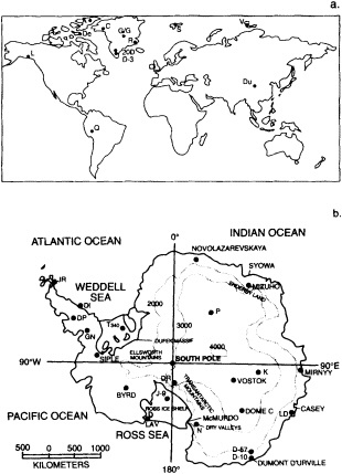
Figure 2
Global distribution of intermediate and deep ice cores and ice-core records. For the Arctic and lower latitudes: A— Agassiz ice cap, C—Camp Century, D-3—Dye-3, G/G—GISP2 and GRIP at the Greenland summit, De—Devon Island ice cap, Du— Dunde, China, L—Mt. Logan, Q—Quelccaya, Peru, R—Renland, S—Svalbard, V—Vavilov Dome, Severnaya Zemlya, 20-D— Greenland. For Antarctica: DI—Dolleman Island, DP—Dyer Plateau, DR—Dominion Range, D-10 and D-57—Dumont D'Urville-Dome C traverse, GN—Gomez Nunatak, JR—James Ross Island, J-9—Ross ice shelf, K—Komsomolskaya, LAV-—Little America V, Ross ice shelf, LD—Law Dome, N—Newall Glacier, P—Plateau, T340—Ronne-Filchner ice shelf. (Source: World Data Center A for Glaciology (Snow and Ice), 1980, 1989.)
from a few low-latitude, high-altitude sites (Thompson et al., 1986, 1989; Thompson, 1992; Holdsworth and Peake, 1985; Holdsworth et al., 1992; Mayewski et al., 1993a). The tropical Quelccaya ice cap in the Peruvian Andes (13°56'S, 70°50'W, elevation 5670 m) provides a 1500-year record with annual resolution of variations in accumulation, oxygen isotopes, chemistry, and dust. In Quelccaya the period from about A.D. 1500 to A.D. 1900, corresponding with that of the Little Ice Age in northwest Europe, is characterized by more negative d18 O values and higher liquid conductivity, while the accumulation was above average in the first part of the period and below average in the second (Figure 3a:
TABLE 2 Properties Measured in the GISP2 Core and the Environmental Information Obtained
|
Property |
Environmental Information |
|
Gas Content |
|
|
Total gas content |
Paleo-elevation of the ice surface |
|
CO2 concentration in occluded air |
Greenhouse gas; increases with temperature; positive climate feedback |
|
CH4 and other trace-gases like N2O, CH3Cl and light hydrocarbons |
Greenhouse gases as well as indicators of the oxidizing capacity of the atmosphere |
|
O2/Ar and N2/Ar ratios |
Fractionation of gases trapped in ice, Dole effect |
|
Stable Isotopes |
|
|
In gases |
|
|
13C/12C in CO2 |
Relative size of carbon reservoirs |
|
18O/16O in O2 |
O2 cycle, global-ice volume indicator |
|
15N/14N in N2 |
Fractionation of gases trapped in ice |
|
13C/12C and D/H in CH4 |
Source distribution of atmospheric CH4 |
|
In ice |
|
|
D/H and 18O/16O in ice |
Primary paleotemperature indicators; deuterium excess d indicates ocean-surface conditions |
|
Cosmogenic isotopes |
|
|
14C/C in CO2 |
Dating climate and ice up to 30 to 40 kyr, carbon-reservoir changes |
|
10Be, 26Al, 36Cl in ice |
Cosmic-ray production rate, snow accumulation rate, dating |
|
He isotopes |
Cosmic-ray production, crustal He |
|
Chemistry |
|
|
Major anions and cations |
Atmospheric chemistry and circulation, source areas, biogeochemical cycling, biomass burning, sea-ice extent, volcanic events, accumulation and its seasonal distribution |
|
Trace metals (Pb, Ir) |
Sources of trace metals and their variability |
|
Methanesulfonic acid and iodide/iodate in ice |
Biological productivity |
|
H2O2 |
Oxidative atmospheric chemistry, seasonality |
|
Particulate concentrations |
Atmospheric circulation, global dust sources, volcanic events, annual layer counting, marker horizons, interhemispheric correlation |
|
Electrical conductivity |
Air circulation, dustiness, volcanic events, biomass burning events, seasonal cycles, chemical marker horizons |
|
Physical and mechanical properties |
Density, texture, fabric, ultrasound velocity, annual layers for accumulation and dating, stratigraphic continuity and flow deformation, core relaxation, firnification processes |
|
Borehole and surface geophysics |
Airborne and surface ice radar, internal layering, surface strain net for ice flow velocity, accumulation, flow modeling, temperature profile and history, borehole deformation and vertical strain |
|
Atmospheric studies |
Automatic weather stations, atmosphere—snow transfer functions for ions, particulates, isotopes, radionuclides. and gases |
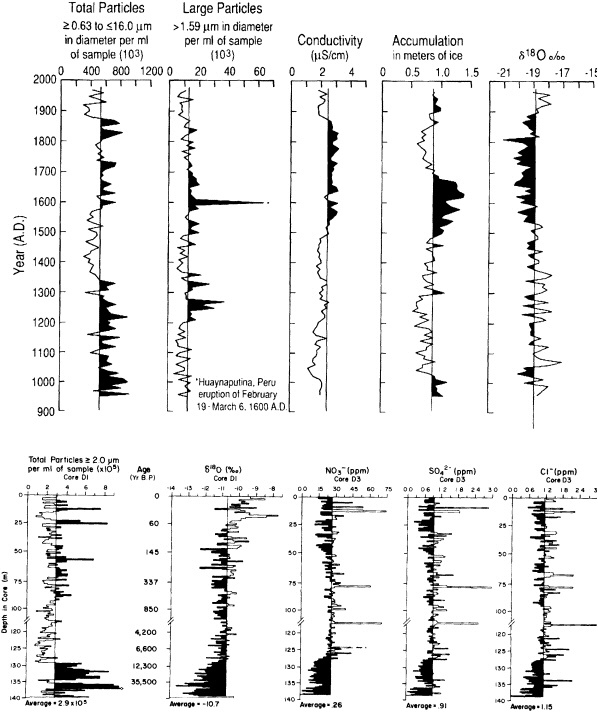
Figure 3
Ice-core records from low-latitude/high-altitude ice caps. Upper group: Dust. conductivity, accumulation, and d18O of the upper part of the 1500-year ice-core record from Quelccaya, Peru (Thompson et al., 1986). An accurate time scale was derived from seasonal cycles in particle concentrations and verified against the historic Huaynaputina eruption of February 19—March 6. 1600 A.D. Lower group: Dust, d18O, and chemistry in the Dunde core, Qinghai-Tibetan plateau, China. The time scale, based on seasonal cycles in particle concentrations and d18O down to 70 m, on visible dust stratigraphy to 117 m, and on ice-flow modeling below 117 m, extends well into the last glacial period (Thompson et al., 1989). (Both figures reprinted with permission of the American Association for the Advancement of Science.)
Thompson et al., 1986). The Quelccaya record is particularly important because long climatic records are rare for the tropics. The accumulation appears to correlate with the recent El Niño/Southern Oscillation record (Thompson et al., 1984, 1992). The Dunde ice cap from the Qinghai-Tibetan plateau of China (38°06'N, 96°24'E, elevation 5325 m) provides the first non-polar ice-core record extending into the last glacial period (Figure 3b: Thompson et al., 1989). The variations in chemical concentrations and dust probably reflect aridity and windiness on the Qinghai-Tibetan plateau and in the Qaidam Basin.
The addition of ice-core records from lower latitudes to those of the polar regions is important for the understanding of global climate variability. First, it allows an evaluation in one medium (ice cores) of the latitude-dependent expression of global climate changes over a considerable range of latitudes. Second, ice cores outside the polar regions allow a comparison between the record of past climate changes in the ice and those in other media such as tree rings, lake sediments, loess, and peat bogs from the same geographic area, albeit at lower elevations. The potential for obtaining more non-polar ice core records exists in a number of the high mountain ranges of the world.
POLAR ICE CORES: THE GREENLAND SUMMIT
Many ice cores have been obtained in the Arctic and Antarctic over the past decades (see Table 1). Of particular interest for decade-to-century-type climate fluctuations are two ice-core projects that have been under way in the summit area of the Greenland ice sheet since 1989, viz., the U.S. Greenland Ice Sheet Project 2 (GISP2) and the European multinational projects Eurocore and GRIP (Greenland Ice Core Project). Basal, silty ice was reached by GRIP in summer 1992; the basal ice plus about 1.5 m of underlying bedrock was obtained by GISP2 in July 1993. Analyses of the two 3000 + m cores reveal a continuous, high-resolution record of a suite of climate-related ice-core properties (Table 2) in an area that, because of its latitude (72.6°N) and elevation (3200 + m), rarely experiences melting. The GISP2 and GRIP ice core records show in great detail frequent, rapid, and simultaneous changes in many climate-related core parameters, in both glacial and interglacial times (Alley et al., 1993; Taylor et al., 1993; Mayewski et al., 1993c; Grootes et al., 1993; Johnsen et al., 1992a; Dansgaard et al., 1993; GRIP members, 1993). These large and rapid changes are already forcing us to revise our ideas about climate stability. Over the next several years, these cores will contribute greatly to our knowledge and understanding of Northern Hemisphere and global climate change. Because the two cores are located at the current ice divide (GRIP/ EUROCORE) and 28 km (about 10 ice thicknesses) west of the divide (GISP2), they are currently in different ice flow regimes (divide flow and flank flow respectively). Comparison of the two core records makes it possible to identify ice-flow effects and to verify the fluctuations in environmental parameters observed in each core. Such comparisons greatly increase the credibility of any reconstruction of climatic and environmental changes that is based on the core records. I will discuss some of the features of the GISP2 ice core record to illustrate the information obtainable from ice cores.
Recent Climate Fluctuations
The oxygen-isotope records from the Greenland summit area indicate a remarkably constant average climate during the Holocene (the last 10 kyr) (Dansgaard et al., 1993; Grootes et al., 1993; Grootes and White, unpublished data). Yet the d18O record shows significant short-term variability (Figure 4). The d18O values, obtained by calculating mean annual values from the 8 to 10 individual measurements over each annual layer, fluctuate over a range of about 6 permil around a fairly constant mean value of -35 permil
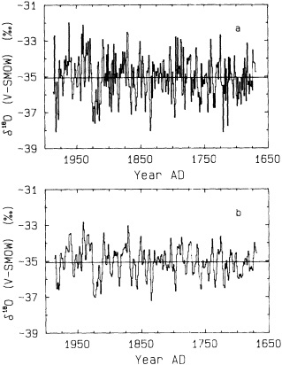
Figure 4
Oxygen isotope record for the upper 100 m at GISP2, Greenland summit. (a) Mean annual d18O values, calculated from about 10 samples per year, on the GISP2 time scale determined from seasonality in visible stratigraphy, ECM, and isotopes (Meese et al., 1994a). (b) The same record smoothed with a simple 3-year moving average.
(Figure 4a). Part of the variability appears to be related to year-to-year weather fluctuations that may be suppressed by smoothing with a simple three-point running mean. This brings out fluctuations on a decadal time scale that have a range of about 4 permil (Figure 4b). With a d18O-temperature coefficient of 0.63 permil/°C (Dansgaard et al., 1973), a range of mean annual temperatures of about 6°C can be inferred. The rapidity and magnitude of the shifts indicate that the fluctuations do not reflect global climate changes, but are most likely attributable to changes in the atmospheric circulation over the summit of Greenland.
For the interpretation of the isotope record in the core it should also be realized that the isotopic composition of precipitation reflects primarily the temperature difference between the ocean surface at which the water vapor formed and the place of precipitation (air temperature at the condensation level some distance above the surface). Thus the isotopes do not provide a simple, direct local temperature record, although the precipitation temperature often dominates. Measurement of the pair of water isotope ratios (2H/ 1H (or D/H) and 18O/16O) in the ice permits the calculation of the so-called deuterium excess, d = dD - 8d18O, that is sensitive to sea surface temperature, relative humidity, and wind speed in the source area of the water vapor over the ocean. Thus it is possible to obtain from the ice-core record information about local temperature changes over Greenland as well as about changes in surface conditions over the Atlantic Ocean (Jouzel et al., 1982; Johnsen et al., 1989).
Application of longer smoothing filters eliminates the decadal fluctuations and reveals weaker, century-scale fluctuations (Figure 5). Interpretation of such filtered records requires great care and needs support from independent environmental evidence to ensure that the fluctuations have physical meaning. Instrumental records from coastal Greenland and the North Atlantic basin (e.g., World Weather Disc, 1990; Dickson et al., 1988b), which are available for about the last 100 years, offer the resolution required for the study of the decadal fluctuations in ice-core parameters shown in Figure 4b. When the rapid fluctuations in isotopes and other properties, observed in the GISP2 ice core, can be related to conditions at the ocean surface and over Greenland and Europe over the last century, then the ice core offers a long, continuous, and detailed record of such conditions. The instrumental record is too short to study century-scale climate variability, so the validation and calibration of the century-scale ice-core parameter fluctuations (Figure 5) will have to come from other proxy records of climate. Such validation is difficult to obtain for the Holocene, because the generally stable climate shows only relatively minor fluctuations that are difficult to correlate. Moreover, few records can match the continuity and detail of the ice cores. Long tree-ring sequences (e.g., Briffa et al., 1992a, b)
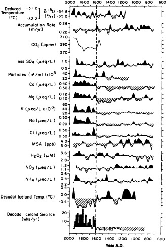
Figure 5
Century-scale variability over the last 1200 years in a suite of parameters measured in the GISP2 ice core from the summit of the Greenland ice sheet. The records have been subjected to a simple 50-year smoothing. Decadal Iceland sea-ice frequency and Iceland temperatures derived from sea ice (Bergthorsson, 1969) have been added for comparison. The time scale was derived by counting seasonal cycles in d18O, visual stratigraphy, and electrical conductivity, and was verified against known volcanic events (Meese et al., 1994a). Accumulation rates were calculated from the annual layer thicknesses corrected for measured density, with a very small correction for ice-flow thinning (Alley et al., 1991). CO2 results were obtained with dry extraction and laser absorption spectroscopy (Wahlen et al., 1991). Concentrations of cations, anions, and H2O2 were measured on biyearly samples (Mayewski et al., 1993b; Drummey, 1993). Methanesulfonic acid (MSA), an oxidation product of dimethylsulfide, indicates biological activity. The time interval includes the northwest European Medieval Warm Period, which extended from approximately A.D. 1000 to between A.D. 1350 and 1450, and the subsequent Little Ice Age, which lasted until approximately A.D. 1900. A significant change in chemistry shortly before A.D. 1600 correlates with Icelandic sea ice, but is not obvious in the d18O record. (From data shared by GISP2 investigators; figure used courtesy of the GISP2 Science Manage- ment Office.)
and varved sediments (e.g., Rozanski et al., 1992) offer possibilities.
Figure 5 shows a 1200-year multi-parameter record from GISP2 subjected to a 50-year smoothing. Records of decadal Iceland sea-ice frequency and of decadal Iceland temperatures derived from the sea-ice record (Bergthorsson, 1969) have been added for comparison. The period covered includes the Medieval Warm Period (MWP), from about A.D. 1000 to between A.D. 1350 and A.D. 1450, and the Little Ice Age (LIA), from about A.D. 1450 until about A.D. 1900, as defined in northwest Europe. The Icelandic record shows clear warm and cold periods corresponding to the northwest European MWP and LIA. The GISP2 d18O record, on the other hand, shows no clear, sustained evidence of the MWP and LIA. Rather, it shows a pattern of minor, century-scale fluctuations throughout this part of the record. During the period of the LIA the warm phase of these fluctuations appears to be more subdued, giving on average a colder climate. A similar observation was made at Crête, Greenland (Dansgaard et al., 1975). Accumulation, determined by identification of individual annual layers and flow modeling (Alley et al., 1993; Meese et al., 1994b), decreases after about A.D. 1200 and is, on average, lower during the LIA period. Terrestrial source indicators such as particles, Ca, Mg, and K, as well as marine indicators such as Na and Cl, are low during the early part of this period (MWP and early LIA) and increase around A.D. 1600, indicating increased transport by stronger winds since A.D. 1600 (see Mayewski et al., 1993b). Particles can also be of volcanic origin, in which case they are accompanied by elevated levels of non-sea-salt sulfate, and may include volcanic glass shards. The non-sea-salt sulfate, which reflects primarily volcanic input as plotted here, does not indicate that volcanism was a major factor in LIA climate (Mayewski et al., 1993b). Concentrations of nitrate (from lightning and soil exhalation, for example) and methanesulfonic acid (MSA, from oxidation of ocean-produced dimethylsulfide) decrease around A.D. 1350 and A.D. 1430, respectively, coinciding with the transition from the MWP to the LIA in Europe. Ammonium, which reflects primarily biomass burning as plotted here, shows high values during periods of climate (and, presumably, vegetation) change.
The multi-parameter ice-core data thus reveal a far richer and more detailed picture of climatic changes and the accompanying environmental alterations during the MWP and ensuing LIA than was available from other sources. This highly detailed record extends back through the glacial-to-interglacial transition well into the last glacial period. The significance for society of the relatively minor climate fluctuations observed in the recent GISP2 ice core record is dramatically illustrated by the fate of the Norse colonies on Greenland that thrived during the MWP from about A.D. 1000 to A.D. 1300, but lost contact with Iceland and disappeared when climate deteriorated after A.D. 1400.
The Glacial-to-Interglacial Transition
Figure 5 shows coherent patterns of change in various properties in the recent record. Yet it is difficult to study the dynamics of comparatively small century-scale climate changes in the presence of much larger short-term climate fluctuations that are not yet understood. A better situation exists across the last glacial-to-interglacial transition, which is apparent between 1670 and 1800 m of depth in the GISP2 core. There the ice has preserved in great detail a record of various climate parameters that show rapid century-scale fluctuations during this period of major climate change. A detailed time scale for the core is being constructed from the annual layering observed in visual stratigraphy, in the electrical conductivity (ECM), and in the particle concentrations of the ice (Alley et al., 1993; Meese et al., 1994a). This will provide the core with an internal time scale with annual resolution for determining the relative timing of the changes in climate-related core properties, such as stable isotopes, chemistry, dust, ice fabric, and atmospheric gas and isotope composition, during the transition from glacial to interglacial climate.
The d18O record of the glacial-to-interglacial transition (Figure 6) clearly shows the Younger Dryas as the last period of full glacial, low d18O values before the Holocene, lasting from about 11.6 to 12.9 kyr BP (Alley et al., 1993). The Younger Dryas is preceded until 14.7 kyr BP by a period of ''warmer" but not fully interglacial climate, probably corresponding to the Allerød/Bølling interstadial complex described in Europe (Mangerud et al., 1974). The interstadial is interrupted by three brief (about a century) cooler episodes, of which the middle one is fairly weak. The ECM record (Taylor et al., 1993), which is measured continuously along the core with a resolution of 1 mm per sample, shows a pattern of highs and lows quite similar to those of the d18O, except that ECM values drop to almost zero during periods of low d18O. The second, weak, cold period of the Allerød/Bølling is not clearly developed in the ECM. The ECM records the presence or absence in the ice of alkaline dust that neutralizes the acid responsible for most of the electrical conductivity of the core (Taylor et al., 1992); it is thus strongly anti-correlated with the calcium concentrations (Mayewski et al., 1993c) in the ice.
The high-Ca, high-dust/low-ECM, low d18O combination in the Younger Dryas indicates a cold climate with strong winds. This finding, which is supported by other terrestrial and marine source indicators such as Mg, Na, and Cl (Mayewski et al., 1993c), fits the general concept of increased meridional temperature gradients and atmospheric circulation during glacial times (Manabe and Hahn, 1977). Comparison of the three Allerød/Bølling cool phases shows that while d18O and Ca concentrations assume intermediate values, the ECM drops to near zero in the two colder ones and shows little change in the third. This is as expected for
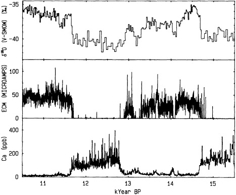
Figure 6
The last glacial-to-interglacial transition (11.6 to 14.7 kyr BP, Alley et al., 1993; Taylor et al., 1993) is indicated by d18O, electrical conductivity (Taylor), and calcium concentrations (Mayewski) in the GISP2 core from the Greenland summit.
a neutralization/titration of acidity. The accumulation over this period, determined from visual stratigraphy (Alley et al., 1993), closely resembles the ECM and the d18O records; it shows a drop to half its Holocene value in the Younger Dryas. Excellent agreement exists between the GISP2 records and the GRIP record (Johnsen et al., 1992a; Grootes et al., 1993).
Particularly interesting in all the records is the rapidity of the climatic changes. Transitions between the high (warm) and low (cold) ECM sections in the core are abrupt; they occur in less than 10 years, sometimes in as little as 3 years. Several transitions show an oscillatory behavior in which the ECM returns rapidly if briefly to pre-transition values (Taylor et al., 1993). Changes in accumulation (Alley et al., 1993) and in chemistry (Mayewski et al., 1993c) appear to be equally rapid. The isotopes have so far been measured only at 1 m (15- to 50-year) resolution, so they still lack this level of detail. Samples cut at 0.6 to 1.7 cm resolution are awaiting a detailed isotope study of these transitions.
The ice-core record of the glacial-to-interglacial transition thus shows an extremely dynamic climate system, with frequent alternations between warm and cold periods of varying length and with major changes in atmospheric circulation occurring over less than a decade (see Mayewski et al., 1993c). Recent work on high-sedimentation rate ocean cores in the North Atlantic (Lehman and Keigwin, 1992; Lehman, 1995, in this chapter; Ruddiman et al., 1977; Sarnthein et al., 1992; Vogelsang, 1990; Veum et al., 1992; Karpuz and Jansen, 1992; Broecker et al., 1990a; Eglinton et al., 1992) shows corresponding changes in the ocean.
The deeper part of the GISP2 and GRIP records (Johnsen et al., 1992a; Dansgaard et al., 1993; GRIP members, 1993; Grootes et al., 1993) shows that major, rapid climate fluctuations were not unique to the last glacial-interglacial transition, but occurred throughout the glacial and even interglacial periods. The pattern of interstadial and stadial episodes in the glacial part of the core provides evidence for frequent changes between cold glacial and nearly interglacial conditions during a time when the deep-sea isotope records (Martinson et al., 1987; Imbrie et al., 1984) indicate the existence of large continental ice masses. This pattern has been observed, although not in the same detail, in all long ice-core records in Greenland (Johnsen et al., 1992a). Major rapid changes during this time are also documented in Atlantic ocean cores (Broecker et al., 1990a; Sarnthein and Tiedeman, 1990), albeit at lesser resolution. A question still to be answered is whether corresponding climate changes exist in Antarctica.
CONCLUSIONS
The new ice-core records being obtained from the summit of the Greenland ice sheet promise to provide a 200,000-year history of changes in climate and environmental conditions over the Greenland ice sheet and in the North Atlantic basin, in unprecedented detail. To utilize this information for the determination of global climate and its variability on all time scales, we need to find first the spatial variability in the ice-core properties, and second the relationship between the ice-core records and paleoclimatic records from ocean sediments and terrestrial sources elsewhere on the globe. For the first we must study ice cores from different parts of Greenland and the Arctic, from lower-latitude, high-altitude ice caps, and especially from Antarctica. For progress toward the second, active collaboration among the glaciologic, the oceanographic, and the terrestrial paleoclimate research communities is needed. In view of the many and very rapid climate changes observed in the ice-core record, it is crucial to obtain accurate and detailed independent time scales for all paleoclimate records so that they can be used in intercomparisons. The detailed information on past changes in climate and environment will then allow us to study not only the major glacial-interglacial climate changes but also climate variability on decade-to-century time scales, and to develop an understanding of the causes and mechanisms of such changes.
ACKNOWLEDGMENTS
This work was supported by NSF grants DPP-8822073 and DPP-8915924, Division of Polar Programs. I thank my GIPS co-principal investigators and L. G. Thompson for contributing their results, and P. A. Mayewski for critical comments.
Discussion
WALLACE: Are there cores from ice sheets in other Northern-Hemisphere locations, such as Alaska, comparable to these Greenland cores?
GROOTES: There are several cores from ice masses in other Northern Hemisphere locations, though none of them is as long and detailed as the Greenland cores. A core drilled by Holdsworth on Mount Logan in Canada provides a record of about 1000 years. Of the three lower-latitude cores drilled by Thompson, the tropical Quelccaya ice cap in Peru covers about 1500 years, and the two cores in China, Dunde and Guliya, go back well into the last glacial period. Also, there are cores in the Canadian Arctic on Devon Island and the Agassiz and Barnes ice caps, and others on Svalbard, Novaya Zemlya, and Severnaya Zemlya. Several of these cores come from lower elevations that have summer melting, so the climate record is less well preserved.
BRYAN: Do the earlier cores, like those Dansgaard analyzed, correspond with your findings?
GROOTES: On a large scale we found the d18O and conductivity of the ice to be quite close for the different cores. In details, though, you find quite different signatures for the various locations. To understand the details of atmospheric circulation, we need a multitude of cores from different locations and elevations so we can distinguish local phenomena and more general patterns. The Quelccaya records in the Southern Hemisphere go back about 1500 years, and I'd say there's the potential in the high Andes for going back to 2000 years.
Temporal Change In Marine Ecosystems
JOHN A. MCGOWAN1
ABSTRACT
Natural populations are highly variable in space and time, so biogeochemical processes and events must also be. Population and community biologists have shown that internal dynamics in biological systems, such as those due to competition and predation, can cause some of the population changes observed. It is generally conceded (but seldom demonstrated) that climatic variations also influence population growth or decline. In addition, harvesting, pollution, and habitat destruction are important agents of change. It is difficult to separate the influences of these several causal factors, so ascertaining the effects of climate change on organized living systems (ecosystems) is not straightforward.
The prevailing approach to the determination of the causes of population variability and ecosystem change is essentially reductionist. There have been many small-scale, local studies of the natural history, physiology, behavior, or growth of single species. But species populations in nature are constantly interacting with a complex system of other species and to broad spectra of physical and chemical variables. Many ecologists have therefore chosen to make the simplifying assumption that different species can be aggregated into functional groupings of species, the dynamics of which adequately represent the state of the biotic system. The group dynamics actually studied, however, are usually the rates of transfer or "flux" of carbon, nitrogen, or calories between a few aggregated categories.
Many ecosystem models assume a steady state. But the systems seldom seem to be in a steady state when field studies are done, and concurrent measurements of "fluxes" involve only a limited number of groups. Ecosystems are organized on very large spatial scales, and the heterogeneity of the ocean makes it difficult to extrapolate upward from small scales of study. Furthermore, the roles of external forcings that are independent of population density, such as climate, are seldom evaluated empirically.
As a consequence, we have little good conceptual insight into how climate affects populations or ecosystems, and almost no predictive capability. But large-scale, long-term monitoring of both individual species populations and aggregated groups has been done. In general, when harvestable populations have been monitored, the relationship between population variations and climate is vague at best. Monitoring of unharvested pelagic systems, however, clearly shows the relationship between population and low-frequency climatic variations.
INTRODUCTION
Laymen always ask how climatic variations will affect commercial fish stocks or agriculture. Climatologists and oceanographers are seldom able to answer. And yet almost everyone believes that there is a strong linkage between climatic variability and biology, especially population biology. Establishing the nature of this linkage in the case of the ocean has proven to be very difficult, and at present we have little predictive ability. This inability is due partly to the approach biologists have taken to the problem, partly to the inherent difficulties in studying the complex, flexible webs of natural biological systems with their numerous feedback loops, and very much to problems of scale.
We are just beginning to understand that different population phenomena happen on different scales for different reasons (Haury et al., 1978). It is the larger spatial scales and low-frequency temporal scales that seem to be the most important, because most of the variability resides there
(Figure 1). But so few observations have been made on the larger scales that even this observation may be tenuous. It does seem true, however, that conclusions of studies of short-term, local changes or functional processes cannot be categorically extrapolated upward and outward to achieve large-scale understanding. The ocean and its populations are too rich in temporal and spatial variability for that to be so. Figure 1 shows typical time/space coverage of most studies designed to measure functional aspects of the ecosystem, such as the flux of energy or materials through selected categories of the biota. Sample separation on such studies may be on the order of hours to about 40 days—the maximum duration of most oceanographic cruises. Although such cruises may be repeated, there is seldom continuity between them, and there are large gaps in the frequency bands we wish to resolve. Variations on the decade-to-century scale cannot be resolved by studies done on smaller frequencies.
There have always been good reasons to study population
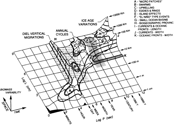
Figure 1
A diagram showing the relationships in space and time of variations in zooplankton biomass. Short-term variations generally take place on small spatial scales. Longer-lived variations are widespread. Different scales of variability almost always have different causes. For example, spawning aggregations, called "swarms," occur in euphausiids. These differ in kind from aggregations due to "upwelling centers" or Gulf Stream cold-core rings. The shaded area on the left indicates the time and space coverage of most process-oriented studies and the resolvable variance. The shaded area on the right is the decade-to-century time scale (data from Haury et al., 1978).
dynamics on the scale of generations, for it usually takes generations for detectable population growth to occur. Also, it has always been acknowledged that somehow or other the environment, including climate, must play a role in affecting population dynamics. Organisms can adapt and acclimate to changing environments. But now it seems that important climatic changes may occur much more rapidly than those experienced during the evolutionary history of most natural populations. If we are to make judgments about the seriousness of the threat of climate change, we will require a much better understanding of how relatively rapid climatic change affects populations, ecosystems, and biogeochemical cycling. It is the 10-to-100-year time scale over which significant changes in population growth rates may be detected, so it is the one that should be studied for most macroscopic organisms.
Feedback loops exist between the biota and atmospheric gases (Figure 2). Rapid climatic change will almost certainly perturb the structure of marine communities and therefore the feedbacks, but for the most part we do not know what direction these perturbations will take or of what magnitude they will be. Carpenter et al. (1992) have shown how changes in the structure of plankton communities in lakes can have significant consequences for nutrient cycles and thus the stability, resilience, and resistance of ecosystems.
It seems essential to begin the process of acquiring the information that will lead us to a better understanding of the role of climate as it affects population and community

Figure 2
The ocean-atmosphere carbon cycle. Dissolved CO2 and O2 in the mixed layer are usually in equilibrium with the atmosphere. Photosynthesis in the upper, lighted zone removes dissolved CO2 and "fixes" carbon into organic compounds. Some phytoplankton secrete calcium carbonate thecae which fall out of the mixed layer and either dissolve or form vast amounts of sediment. Plants also produce dissolved organic matter and particulate organic detritus which may sink. Much of the organic carbon produced is eaten by animals and passed through the food web (see Figures 3 and 4). Animals also produce dissolved and particulate organic matter. Some zooplankton engage in a diel vertical migration, feeding in the mixed layer and respiring and excreting in the sub-thermocline waters. Physical downwelling carries with it dissolved inorganic and organic carbon and detritus. Detritus is fed upon by microorganisms which through the process of respiration remove oxygen and add carbon dioxide to the sub-thermocline water. These waters are greatly oversaturated with CO2 and undersaturated with O2 everywhere. The sediment and the sub-thermocline waters of the world's ocean are the two greatest reservoirs of carbon on earth. Upwelling of oversaturated intermediate water may complete the cycle. The relative importance of the biological portions of this cycle is unknown.
biology. Time-series monitoring of critical but measurable components of large natural systems is needed to achieve this understanding. Limited efforts in this direction have already yielded important results.
BACKGROUND
Ecologists and other biologists want to understand why populations vary so widely in time and space. The scales of interest extend to geological time, which includes extinctions, speciation, and therefore evolution and the origins of diversity. Malthus in 1798 pointed out that all organisms could more than replace themselves during their lifetime, but that the resources (food, space, light) necessary to sustain such implied population-growth rates were in short supply. If essential resources are limited, not only individuals but species populations must compete for those resources. Observations of such competition led Darwin to propose a natural selection in favor of the fittest competitors. Ever since, competition theory has been a mainstay of the most fundamental concepts in ecology and evolution (Lotka, 1926; Volterra, 1926; May, 1973). This interplay between competitors can be shown in models and experiments to yield oscillations in population sizes.
One important outcome of these studies was the recognition that the relationships between the population growth rates of two or more competing species must be density dependent (i.e., non-linear) in order to stabilize the system. Stability allows for the continued presence of all of the species involved, and thus the persistence of diversity. The latter is an observed fact of nature. A very similar conceptual basis exists for predator-prey interactions with density-dependent, non-linear relationships between population growth rates required for dynamic equilibria of the two (or usually more) interacting populations.
Empiricists working with real, complex biological systems in nature often question the utility of such models. Not only species interactions (as predators, prey, and competitors) but demographic structure, genetic structure, stochastic factors, and in particular external non-density-dependent environmental forcing (i.e., climate) play very important roles. All exert their effects concurrently in complex, species-rich systems where everything seems to depend on everything else. This makes the models difficult to test. There are, unsurprisingly, few well-documented cases in nature showing competitive exclusions, or demonstrations of environmental variations' changing the course of a competitive contest. Some relatively short-term (in terms of the generation times of the subjects) experiments in removal or exclusion (of predators) have been done, but, as Pimm (1991) has pointed out, often not enough time has elapsed for effects, expected or otherwise, to appear. For these species-removal experiments to be useful for full validation of competition, predation, and community theory, the effects on populations must be followed for the generations it takes for differences in population growth rate to be detected and to influence other species' population growth rates (e.g., through competition). For many marine organisms of interest, decades are required.
In the cases where adequate time-series measurements of population sizes of pelagic organisms have been obtained, the largest, and therefore the ecologically most important, changes have been found to be low frequency, mainly interannual. This result holds despite the organisms' intrinsic generation times, which may differ by orders of magnitude between species.
PERTURBATIONS AND CHANGE
The difficulties in applying competition/predation theory in the attempt to understand the configuration or kinetics of natural, multi-species communities have led to the development of an additional body of theory that depends on either external disturbances that perturb the system or the existence of patchy, non-random aggregations (Paine and Levin, 1981; Yodzis, 1978). In both cases the expectation of having a superior competitor present in the system, e.g., the competitive exclusion of others, is mitigated. This happens because the superior competitor's populations are episodically diminished by disturbances, thus allowing the inferior competitors to persist. The inferior ones may have special adaptations to allow them to reproduce at an early age or to disperse well, or have some other opportunistic trick that allows them to continue as populations while co-occurring with competitors. This may happen if density-independent perturbations occur that inhibit the dominant competitor (e.g., storms). Patchiness can also work, in theory, if there is constant or at least frequent migration between patches of species or groups of species with varying competitive abilities. This leads to a sort of contemporaneous disequilibrium (Richerson et al., 1970). Observations have been made, particularly in tropical forests and the intertidal zone, that are consistent with these theories and tend to support them. However, few sets of observations cover the necessary number of generations (particularly in forest trees). Furthermore, almost all of the studies have been done on sessile species, where space is clearly a strong limiting resource. There is evidence (McGowan and Walker, 1985; Venrick, 1990) that mobile oceanic populations and communities may not behave in this way.
This body of theory explicitly includes forcing from outside the biological system in a way that is independent of population density. The primary extrinsic force is climate, which is not generally thought to be affected by intrinsic biological processes, even though there are feedbacks from oceanic biota to the atmosphere as shown in Figure 2.
There is consensus that climatic variation is of central importance in the regulation of the availability of resources,
the intensity and even direction of competitive contests, and the success of prey populations in overcoming the effects of predation. It is not clear why this outlook has developed. Perhaps it is because population cycles are clearly linked to the seasonal cycle, which is a well-understood climatic phenomenon. Other lower- (and higher-) frequency climatic events are also sporadically invoked as sort of a deus ex machina, although they are not often clearly shown to cause or to be linked to population changes in a predictable or quantifiable way. There is no well-developed body of theory of climatic effects, other than those of temperature on the fecundity or metabolic rate of individuals. But the study of the functional response of an individual to, say, temperature change cannot be extrapolated to yield information on the numerical response of entire populations, whose increase or decrease depends on the ratio of birth rates to death rates.
COMMUNITY STRUCTURE, TROPHIC STRUCTURE, AND CHANGE
Organized pelagic ecosystems do exist, and can be shown to have natural boundaries. They occupy regions that are physically distinctive. They are large, few in number, and relatively simple by comparison with land ecosystems because there are fewer constituent species (McGowan, 1971). But in spite of their relative "simplicity," they all contain hundreds of species populations of producers, herbivores, carnivores, omnivores, and degraders. Each of these species populations is thought to be genetically unique, having its own life-history pattern, physiology, and behavior. Since the species of these systems have spatial and temporal overlapping distributions, they all form nearly constant parts of each other's biotic environment. There is plenty of opportunity for interaction, so they are all more or less interconnected dynamically through nutrient exchange or competitive or predator-prey linkages.
There are significant logistic difficulties in studying the dynamics of such complex ecosystems on the basis of their individual species' population dynamics or physiology. Conceptual or mathematical models resulting from such ecosystem studies are often intractable (Hedgepeth, 1977). Ecologists, especially marine ecologists, have therefore resorted to the study of aggregated categories or functional groupings, such as "primary producers" or "herbivores" (see Figure 3), thus reducing the number of entities (or terms). Such approaches have little to do with species competition or predation theory, but nevertheless have theory of their own (Lindemann, 1942; Steele, 1974; Fasham, 1984): For example, trophic theory attempts to explain variations in abundance of entire trophic levels (primary producers, herbivores, pelagic fish). These are aggregated categories of species either shown, or more often assumed, to have the same or similar trophic (i.e., food) requirements. The rates of transfer between levels, either of energy or of
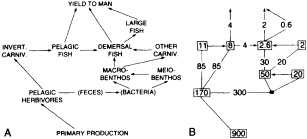
Figure 3
(a) A North Sea food web in which the details of the organization have been aggregated into major, trophic categories. (b) The values in the boxes indicate the "assimilation" in kcal m-2 yr-1; the arrows show input or "flux", also in kcal m-2 yr-1. In this model Steele has emphasized the efficiency of energy transfer between boxes and the stability of the system. He was concerned about the difficulty of making suitable observations at sea. (After Steele, 1974; reprinted with permission of Harvard University Press.)
some nutrient such as nitrogen, and the efficiency of these transfers are what is measured. But models based on nutrient flux usually include only one variable, and they differ conceptually from energy-flow models. Nutrients are retained and recycled, energy is not.
Pelagic ecosystems may be very far from equilibrium, and indeed they never seem to be in steady state when the measurements are made. The complete suite of pertinent fluxes within the food web have never been measured at the same time. Transfer rates must be non-linear and density dependent to stabilize the system. Determining a sufficient number of such rates to describe the state of the systems in nature has proven to be very difficult. Furthermore, ascertaining how extrinsic perturbations or variations in climate may change these rates seems as yet to be beyond current capabilities. The problems are likely to remain until the rates of change of biomass for the aggregated categories (i.e., the trophic levels) have been measured over a length of time sufficient to include some biologically "important" climatic events. Similar difficulties arise in attempts to model the role of the marine biosphere in the global carbon cycle. For this task one must understand how oceanic food webs withdraw CO2 from the surface waters, package it as organic parcels, and export it to the subpycnocline waters (Figures 2 and 4). This process sequesters millions of gigatonnes of carbon (GtC) in the sediments and tens of thousands of Gt as dissolved inorganic and organic carbon in the intermediate and deep waters of the world's oceans. But our understanding of the rates of transfer between what are assumed to be the important aggregated categories (boxes in Figures 2 and 4) is very meager (Longhurst, 1991; Sundquist, 1993). In most cases we cannot estimate the error in these rates, and have little idea of which kinds of extrinsic perturbations will alter them.
Time series of concentrations of the most easily measured
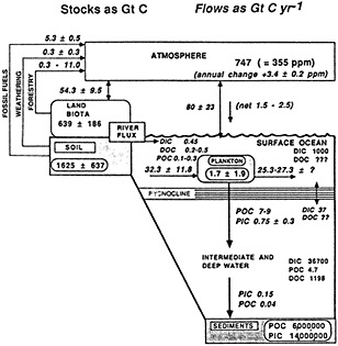
Figure 4
A diagram of the global carbon budget, showing what are thought to be the most important pathways between stocks or transient reservoirs. An attempt has been made to assign values to the amount of carbon in each reservoir (in GtC) and the flux of carbon between them (in GtC yr-1 ). Varying levels of uncertainty are associated with these values; many are essentially unknown (Sundquist, 1993). Many or perhaps most of the fluxes are non- linear, and few of the reservoir sizes have been followed through time. Some known mechanisms of flux are not included—for exam- ple, the advective sinking of particulate organic carbon shown in Figure 2. (After Longhurst, 1991; reprinted with permission of the American Society of Limnology & Oceanography.)
quantities, along with climatic variables, are needed to allow us to at least describe a system's response (or the lack of it) to perturbations, and to promote realistic modeling efforts and their validation. We do not, at present, really know what types of atmospheric or hydrographic perturbations affect biological systems and what types do not. There are many kinds of disturbances and perturbations, ranging from microscale turbulence to El Niños, almost all of which have been implicated one way or another. Some of these seem to represent severe disturbances, whereas others do not. Which ones, then, are which? How, and in what directions, do the systems respond to different kinds of climatic events (Wiebe et al., 1987)?
FISHERY DATA
Some marine populations have been followed very closely over many generations. A great many detailed studies have been made of the population dynamics of commercial and sport fish, because of their obvious importance to man. These studies typically focus on populations of single species that were targeted because of economic or political pressures, and because the catch itself constituted a convenient and useful population-sampling tool. The almost universal result, where long-term studies were done, is that individual species' population sizes vary enormously through time, frequently by factors of ten or more, and that they do not often correlate with each other or with anomalies in climatic proxy measurements such as sea surface temperature (Garrod and Colebrook, 1978; MacCall and Prager, 1988; McGowan, 1989; Skud, 1982; Steele and Henderson, 1984; Sund and Norton, 1990; see Figures 5, 6, and 7). But Kostlow (1984) has pointed out that if the number of fish larvae and juvenile survivorship (hence recruitment to adult stocks) depend on large-scale environmental variations, there should be correlations in recruitment among species of fishes whose larvae have overlapping large-scale distributions, since they would be expected to respond in similar ways to perturbations. Kostlow examined time series of recruitment in 14 stocks in the northwest Atlantic; out of 91 comparisons in his correlation matrix, fewer than one-half were significant and 35 were negative. He also examined relationships between stock and recruitment and found no evidence for density dependence, and on this basis concluded that large-scale extrinsic processes were likely to be responsible for those correlations observed. However, no physical or climatic data were used in the study, and apparently no corrections were made for multiple testing in his correlation matrix.
Hollowed et al. (1987) examined pairwise correlations of 35 years of recruitment data for all possible pairs of 59 species or stocks from the northeastern Pacific. When they applied a correction for multiple testing, very few of the pairwise correlations were significant. One of their conclusions was that the principal value of the correlation patterns seen in their study lay in the possible use of the patterns for generating hypotheses about factors influencing recruitment. Garrod and Colebrook (1978) looked at recruitment patterns of many species over large sectors of the North Atlantic using principal-component analyses, but failed to find meaningful general patterns. Sund and Norton (1990) have examined the time series of California fish landings for the period 1928 to 1985. They tested the utility of the data set in relating variability in landings to climate variability for warm-water species (Figure 5). Only one species of the seven was associated with temperature variations other than seasonal. Sund and Norton conclude that "data concerning any resource highly impacted by man's economic or other activities are likely to have variability in amplitudes and frequencies that are greater than those induced by non-anthropogenic factors. Declines in fish landings as a possible result of high exploitation during warm water periods and high abundance is thought to be a major factor which confuses simple interpretation of the data." Steele and Henderson (1984) point out that some of the most dramatic population
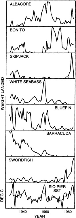
Figure 5
The annual landings of some important warm-water commercial and sports fish in the California Current, along with sea surface temperature (and its 5-year running mean) at Scripps Institution of Oceanography's pier. Each panel is scaled to give the maximum weight landed at full scale. (From Sund and Norton, 1990; reprinted with permission.)
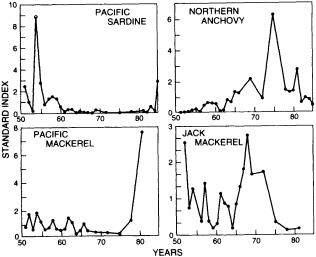
Figure 6
Variations in abundance indices of the larvae of four important schooling fish off California. These fish (Pacific sardine, northern anchovy, Pacific mackerel, and jack mackerel) have broadly overlapping distributions and very similar diets. (After MacCall and Prager, 1988; reprinted with permission of the California Cooperative Oceanic Fisheries Investigation.)
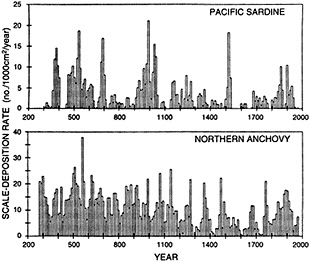
Figure 7
A composite time series of fish-scale deposition rate in the Santa Barbara basin.
fluctuations occur in pelagic fish stocks, but there are no obvious or simple general relationships between these and contemporaneous variations in climate or physical changes in the ocean. They claim that abundance changes are rapid, but tend to occur following 50-year periods of relative stability. Steele and Henderson suggest (through the use of a model) that fish populations are resistant to environmental pressures until they reach a certain threshold, at which point they flip over to a new relationship with their environment; in other words, they show multiple steady states.
Although multiple steady states may exist, many factors besides population size influence catch data; these include fishing-gear changes, the amount of fishing effort, and market-demand factors. Furthermore, most commercial species show long-term, secular trends of decreasing abundance (catch) that are not associated with climatic trends. There are strong indications that human harvesting of populations has introduced such a large added source of mortality at such an unusual point in the age structure that natural and climate-induced variability may be masked. Thus, the use of fisheries catch data (or other estimates of population change) to test competition and predation theory, or to assess the role of extrinsic, density-independent factors such as climate, is questionable. In this case anthropogenic and natural variability cannot be separated, and long-term studies of unharvested, co-occurring species of fish are clearly called for.
FINE-SCALE SEDIMENTARY RECORDS
In an attempt to assess anthropogenic influence on fish populations, Soutar and Isaacs (1974) utilized a time-series of fish-scale counts from cores of the annually varved sediments from the anoxic Santa Barbara basin off Southern California. They looked chiefly at the Pacific sardine and the northern anchovy, two pelagic, schooling species with overlapping distributions in the ocean and almost identical food habits. Judging from 40 years of catch records (meager for the anchovy in the early days) and from egg and larval surveys, the abundances of these two fish had apparently oscillated out of phase. Soutar and Isaacs assumed that the fish-scale count from a core (7.6 cm in diameter) provided a reliable estimate of the abundance of fish in the overlying waters, and that the region of the Santa Barbara basin was representative of the much larger area occupied by these two fish. Their results, which covered at least 1800 years in 10-year increments, showed large oscillations in abundance of both fish as far back as A.D. 400; these variations had a red spectrum, and the two species may have varied in abundance with respect to one another before man began harvesting them. Subsequent studies (e.g., Baumgartner et al., 1992) from this core plus a second one, however, have shown that the two species' abundances are most often positively correlated with one another (Figure 7). Furthermore, attempts to calibrate the sedimentary record, by using 5-year blocks from much larger box cores of sediment from only the past 50 years or so that can be matched to actual in vivo population estimates, have not yielded very convincing results. Baumgartner et al. attempted to overcome some of the sampling problems by time-averaging the data into 10-year blocks and by using only four categories of abundance; they were thus able to resolve only variations of 50-year periodicity. Since both species have generation times of two to three years, these cases have not been very useful for tests of the importance of climate in theories of competition and predation. If those estimates of the lower-frequency variations can be validated, however, they should be examined with respect to the climatic-change indices that can also be found in the cores. That comparison would seem especially apt, since at low frequencies the two species appear to be positively correlated. Such a correlation would be expected if these two ecologically similar fish were sensitive to climatic changes.
Both Lange and Schimmelmann have examined high-frequency signals of several kinds found in Santa Barbara cores, with the goal of recovering climate-related information from the varved sediments in the Santa Barbara basin that have year-to-year resolution (Lange et al., 1990; Schimmelmann and Tegner, 1991; Schimmelmann et al., 1990; Schimmelmann et al., 1992). While in some cases there seems to be low-frequency (several decades) correspondence of climate indicators and biogenic flux, the existence of higher-frequency relationships is not clear.
TIME SERIES OF DIRECT MEASUREMENTS
There is a third body of biological research that has no very structured theory behind it, nor is it concerned with the details of the intermediary mechanisms responsible for population changes. It is empirical and observational. Its main aim, which does not depend on preconceived ideas of how systems function, is to describe complex ecosystems by asking what the temporal scales of variability of basic properties such as climate, hydrography, nutrients, and biological functional groups are. In other words, what are the frequency spectra? With such information, hypotheses may be tested. Are some frequencies more important—i.e., of greater amplitude—than others? Are there regular patterns of succession over time (Wiebe et al., 1987)? Are there connections (i.e., correlations) between climate change and ecosystem change?
The assumption behind the studies that constitute this third body of research is that various components of the physical-chemical-biological systems interact to influence each other's magnitude or concentration over time. If these interactions happen in a patterned or regular way, there should be detectable statistical relationships between them in spite of a large amount of noise. Most of the researchers in this field want to know whether there are cross-correlations and, if so, at which frequencies. Since both density-dependent and density-independent forcing are probable, the fact that this approach avoids the necessity of discriminating between them is in its favor. It does, however, presuppose a series of measurements long enough and frequent enough to sample adequately all of the potentially important frequencies of variation. Since at present there are not many cases in which we know what these are, we must begin with frequent sampling over long periods of time to capture
the essential features of the variations and to lessen the possibility of aliasing. Furthermore, since the ocean is so heterogeneous horizontally, it is critical to separate local variations caused by local, in situ processes or events from variations caused by the advection of water past the sampling site—water that may have had a different (and unmeasured) history. While the number of moderately high-frequency, long-time-series studies of biology of the ocean is small, the number of these in which spatial averaging is possible is even smaller. Spatial averaging can help to ameliorate the effects of patchiness and advective events. A spatially arrayed time series can also be used to determine the correlation length scales of variations, and may also allow discrimination between anthropogenic and natural variations (which will be discussed later).
A few such series of long duration have been examined in this way. In all cases practical considerations have kept the sampling frequencies to monthly or, at best, biweekly intervals. However, two of these, the continuous plankton recorder (CPR) surveys of the United Kingdom and the California Cooperative Oceanic Fisheries Investigations (CalCOFI), are of over 40 years' duration, and both have spatial dimensions.
Continuous Plankton Recorder Surveys
The continuous plankton recorder surveys of zooplankton and phytoplankton species' abundance in the North Atlantic between Scotland and Iceland began in 1939. After World War II, ship routes to and from the Atlantic Ocean weather stations were added to the survey. It was extended progressively until by 1965 a large part of the North Atlantic north of 45°N was sampled monthly by 20 merchant ships and 16 weather ships. In that year, 112,000 miles of continuous sampling was done.
Three early, major results of this effort have been: the preparation of composite biogeographic maps of spatial variations in species abundance and of patterns of diversity in the northern North Atlantic, based on thousands of observations; the derivation of species assemblages and their spatial and temporal trends (i.e., the outlines of community structure); and the analysis of temporal variations in plankton populations. The power of this last analysis is greatly enhanced by the availability of so many samples and the ability to spatially average the data. Much of the recent work on temporal changes has been done for a single area (10°E to 20°W, 45°N to 65°N) comprising part of the northeastern Atlantic, the North Sea, and the English Channel (CPR Survey Team, 1992). This effort has emphasized the relationships between environmental variations and plankton abundance (Figures 8 and 9).
The earlier studies of the CPR group were impeded by the lack of physical and chemical data on commensurate scales of sampling. As time-series information accumulated,
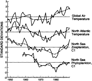
Figure 8
Low-pass filtered Continuous Plankton Recorder and climate data from the Northeast Atlantic. The data shown are anomalies in terms of standard deviations from the mean of a long-term data set. The zooplankton and phytoplankton first-principle components of abundance fluctuations were used here. (From the CPR Survey Team, 1992; reprinted with permission of the International Council for the Exploration of the Sea.)
it became apparent that it was the larger time and space scales that showed the greatest amplitudes of variation; interannual variations were evident, and in some cases dominated the variability. One of the more spectacular of the long-period events was the progressive delay of the spring bloom for phytoplankton species (Figure 9) and a shortening of the seasonal cycles for many zooplankton. Dickson et al. (1988a) relate the declining trend in abundance of both zooplankton and phytoplankton between the mid-1950s and 1980 (the trend may have reversed during the 1980s) to a long-term increase in the northerly wind component over the eastern North Atlantic and European seaboard between 1950 and 1980. They suggest that the consequence of a delay in the onset of the spring bloom of phytoplankton and a consequent shortening of the production season reduced the carrying capacity for zooplankton. The increase in spring winds should have resulted in increased wind mixing, thus changing the critical depth in the sense of Sverdrup (1953). This would mix the phytoplankton beyond the depth at which light is sufficient for photosynthesis to exceed respiration, and thus delay the initiation of net production (i.e., population growth). But Colebrook (1985) associates these trends with variations in west winds. It seems highly likely that in both cases the same basic pattern of climatic change is involved. What is fairly certain, however, is that the changes in the phytoplankton are not a direct response to changes in temperature, and that the
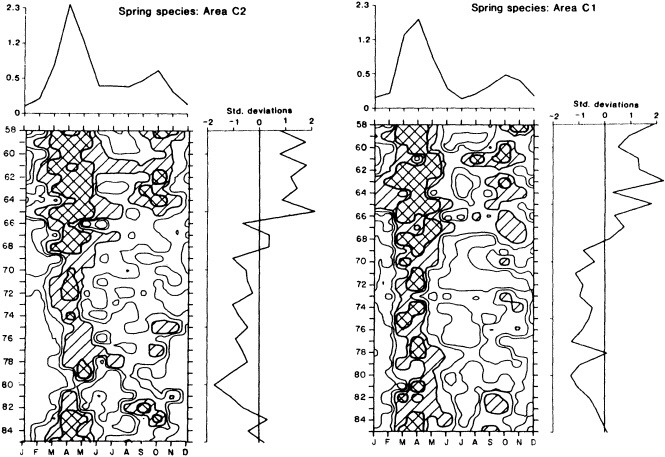
Figure 9
Month/year contour plots, long-term monthly means, and standard deviations of 12 species of phytoplankton in CPR standard areas C2 (west-central North Sea) and C1 (east-central North Sea), 1958-1985. (From Dickson et al., 1988a; reprinted with permission of Oxford University Press.)
pattern of change in the North Atlantic should be considered, from the point of view of plankton, simply as an index of climate change (CPR Survey Team, 1992).
Additional studies of the CPR data (Aebischer et al., 1990; Taylor et al., 1992) have confirmed the very close relationship between large-scale, low-frequency variations in plankton and climate changes. These relationships indicate a climate connection spanning the complete width of the North Atlantic, and support the view that low-frequency, large-amplitude planktonic trends are driven externally (Taylor et al., 1992). Radach (1984) reviewed much of the CPR information to discover how much of the observed change in production cycles could be explained by climate. Spectral analyses imply that at least 50 percent can be attributed to the physical environment. Perhaps density dependent biological processes can account for the rest, but the CPR sampling scheme and sample-processing methods, integrating through time and space as they do, prevent the detection of smaller-scale processes and events that may contribute to the process of change.
The California Cooperative Oceanic Fisheries Investigations
The CalCOFI program is not primarily a fisheries study; rather, it is concerned with all of the elements of the pelagic ecosystem that can be measured routinely. It was the continuing decline of the Pacific sardine that led to the establishment of this large environmental study of the California Current in 1949. The CalCOFI study resembles the CPR work in some important ways. Both allow for the spatial averaging of time series, cover large areas, and are of over 40 years' duration, thus allowing frequencies of change from monthly to decadal to be resolved. Both target the larger, more efficiently sampled zooplankton. They differ in that CalCOFI measures physical and chemical properties in addition to biological ones, and has done so over a greater depth range (500 m), thus adding another dimension to the study.
As in the CPR study, species' biogeographic patterns and seasonal cycles have been described by CalCOFI. There
is a strong north-south gradient in biomass and an offshore, midstream maximum in the California Current. Most of the species present are not endemic, but have much larger populations outside of this current system. Elements of four different, large faunal provinces mix together in the central sector, which results in very high species diversity. Time-series studies (Bernal and McGowan, 1981; Chelton et al., 1982) have yielded important results. Low-frequency interannual variations dominated the spectra of zooplankton abundance, temperature at 10 m, salinity at 10 m, and mass transport from the north. Furthermore, these variables were coherent and well correlated throughout the system (Figures 10 and 11). The changes in temperature and salinity were consistent with the changes in transport from the north, since the North Pacific and Aleutian currents are sources of cool, low-salinity water. These waters also tend to be high in plant nutrients, and their movement down the coast of North America and into the California Current would certainly have a fertilizing effect that should lead to higher
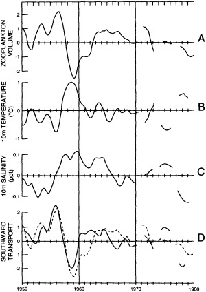
Figure 10
The space-averaged, non-seasonal, low-pass filtered (double 13-month running mean) anomalies of zooplankton biomass, temperature, salinity, and mass transport of the California Current. The dashed line in panel (d) is the zooplankton data, repeated from panel (a). (From Chelton et al., 1982; reprinted with permission of Kline Geology Laboratory.)
biomass. But there is also a normal north-to-south gradient of plankton; during times of enhanced southward transport, this could shift southwards and give the appearance locally of a temporal change in population growth. In either event, this change in growth is clearly associated with whatever climatic changes cause such large-scale shifts in the mass transport of the California Current system.
Bernal and McGowan (1981) found that the CalCOFI plankton anomalies were uncorrelated with anomalies in the most popular index of coastal upwelling. This unexpected result has led to new interpretations of the regulation of biomass and new concepts of which physical events are important and which are not. Standing out in this study are the profound effects of the 1958-1959 California El Niño. The largest negative plankton anomalies of the time series from 1949 to 1980 occurred then. This anomaly was repeated in 1983-1984. Further studies (Roemmich and McGowan, 1995) have brought this time series up to date. In their longer series, covering 1950-1993, a clear warming trend, a negative salinity anomaly, and a 70% decrease in zooplankton biomass are all seen on the interdecadal scale (Figure 11). But there was no such long-term trend in mass transport from the north. During this period, temperature differences across the thermocline increased. The resulting increase in stratification inhibited wind-driven upwelling from sources rich in the inorganic nutrients needed for new production, so zooplankton populations decreased. This proposed mechanism for the interdecadal variations in plankton abundance is quite different from the one proposed for interannual changes (Chelton et al., 1982). A model designed to ''explain" interannual variations would be inappropriate for the interdecadal scale, since quite different mechanisms seem to be involved.
The observed rate of decrease in zooplankton biomass is 6 × 10⁻¹⁰ s-1 over the 43 years of the Roemmich and McGowan (1995) study. On such long time scales, zooplankton biomass is controlled by the net of decreases due to an excess of death rates over birth rates, and increases through advection by currents from the north. Advective input is estimated to be ~5 × 10⁻⁸ s-1, which is far larger than the long-term trend. The trend is a small residual of much larger terms; it cannot be isolated by case-history studies of currents, reproduction, or mortality. It nevertheless is a dramatically large signal when accumulated over 43 years. The Roemmich and McGowan study shows that climate-ecosystem studies dominated by short-term, process-oriented experiments cannot simply be extrapolated to decadal time scales, where the balance of terms is different from monthly or seasonal balances.
Taken together, the CPR and CalCOFI studies have shown clearly and unambiguously that biotic variability in the ocean has a red spectrum, and that the largest anomalies are very closely related to climatic variations. These studies have even allowed us to focus on some intermediary mecha-
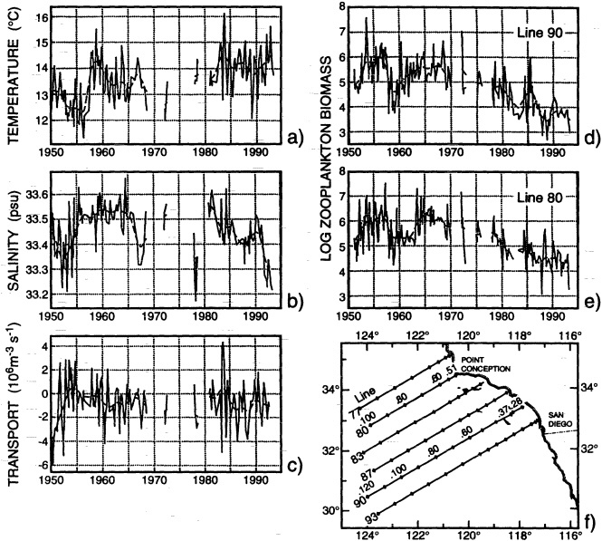
Figure 11
Variations over time in the upper 100 m of the ocean on line 90 (see panel f). (a) mean temperature, (b) mean salinity, (c) transport (in sverdrups, with a 500 m reference level), and (d) zooplankton biomass. Panel (e) shows biomass at line 80 for comparison. (After Roemmich and McGowan, 1995; reprinted with permission of the American Association for the Advancement of Science.)
nisms that seem to be important, and to reject others that seem less so.
Allen's Scripps Pier Data
During the years 1919 through 1939, W.E. Allen took daily samples of phytoplankton from the pier at Scripps Institution of Oceanography, and from 1920 to 1939 a similar time series was taken at Port Hueneme, some 120 miles to the north (Allen, 1941). Other five-year high-frequency series were also obtained at various distances from La Jolla until either they were shown to resemble La Jolla so closely that effort was abandoned, or logistic and financial difficulties arose. Allen tracked the variations in abundance of 98 species of diatoms and over 25 species of dinoflagellates. Population changes of several orders of magnitude occurred both within years and between years. Although he was able to demonstrate a clear seasonal change in both total dinoflagellates and total diatoms, interannual differences obviously dominated the series. Allen lacked the statistical tools to investigate this further, however. He did not analyze the phytoplankton as a community or ask questions about
species diversity shifts with respect to hydrography, for such concepts had not yet been well developed. Tont (1981, 1987, 1989), using Allen's 1930-1939 data, looked at seasonality and seasonal anomalies of 23 of the most abundant species of diatoms. He found negative correlations between a few of the species pairs; some of these appear to be significant, whereas others do not. He also cross-correlated seasonal anomalies of total diatoms and dinoflagellates with sea-surface and air-temperature anomalies. All of these yielded negative coefficients, some of which appear to be significant. Tont (1987) states ". . . at very best, however, climatic change, as defined by the variables used in this study, explains only 36 percent of the total variance. . . ." It is clear from his figures that cold years at the SIO pier are more productive than warm ones.
Sugihara and May (1990) have also used Allen's data (along with those for the incidence of chickenpox and measles in New York City from 1949-1972) to test their approach to making short-term predictions about the trajectories of chaotic dynamical systems. They show that "apparent noise associated with deterministic chaos can be distinguished from sampling error and other sources of externally induced environmental noise." They conclude that the method gives sensible answers with the observed time series of measles (deterministic chaos), chickenpox (seasonal cycles with additive noise), and diatoms (a mixture of chaos and additive noise). The dynamics of diatoms near shore reflect at least partial governance by a chaotic attractor. This result is new and valuable information that could only have come from such a time series. It is an indication of the degree to which the variability of plankton populations is driven by external, density-independent forces rather than by the ecosystem's internal nonlinear dynamics.
NATURAL AND ANTHROPOGENIC VARIABILITY
Most of the biological time-series data come from populations that are strongly influenced by humans, either directly by their harvesting forests, fish, and game, or indirectly through pollution or habitat disruption. Our inability to separate the effects of natural processes from anthropogenic ones has proven to be a serious impediment to progress in environmental management, the testing of theories of ecosystem behavior, or determining the role of climate in population variability. Conversi and McGowan (1994) attempted to make this separation through the use of spectral and time-series analyses of three geographically separated sites with similar kinds of sewage discharge and similar water-quality monitoring programs. Her approach was simple: to examine the relationships between the frequency spectra of sewage discharge and those of water transparency, particle concentration, and temperature within and between sites. Each site (Los Angeles City's wastewater treatment plant at Santa Monica Bay, Los Angeles County's at Palos Verdes, and San Diego County's at Point Loma) had a somewhat different 17-year history of discharge and different mass-emission curves. Conversi found that these were, in each case, uncorrelated with the local water-quality monitoring data. But the water quality did vary with time, especially at the lower frequencies. Most of this variations was seasonal (which the discharge was not), and the rest was correlated between sites and with temperature. There are known natural low-frequency coherent temperature variations in the area of the Southern California Bight. It appears that most of the variations in water clarity (a prime water-quality variable) were natural.
Radach et al. (1990) studied a long time series of temperature, salinity, plant nutrients, and phytoplankton samples taken 3 to 5 days per week at a single station in the German Bight in the southeastern North Sea. They observed conspicuous changes in the annual cycles of nutrients, a general increase in phytoplankton biomass, a shift in the ratio of flagellates to diatoms, and other evidence for a strong systematic change in the ecosystem. There is no evidence for concurrent changes in meteorological or hydrographic conditions. They attribute the observed changes to the anthropogenic increase in nutrient loads of the rivers that discharge into the coastal zone. On the basis of the changes over time in the magnitude, proportions, and pulse-like nature of the nutrient inputs, they suggested anthropogenic mechanisms for the observed shift in the Bight's carrying capacities for different kinds of phytoplankton.
CONCLUSIONS
Relatively few of the time series in the open ocean are of sufficient length and frequency to permit the exploration of important questions of population and community dynamics or the role of climate in influencing these. Many of the series have such large gaps that aliasing is likely, and some frequencies cannot be determined. Others track populations so affected by human activities that it seems unlikely that climate-induced variations can be separated from anthropogenic changes.
However, there are some marine populations for which the sampling has been long-term and of relatively high frequency, as with the CalCOFI and CPR programs. In both cases long-term, space-averaged data have shown that zooplankton variance has a red spectrum and that it is the interannual and interdecadal changes in abundance that are most important, although both study programs showed clear seasonality as well. The low-frequency variability was coherent over large geographic areas in both the Atlantic and Pacific. Both programs have shown significant correlations of plankton-biomass changes with large-scale climatic variations. There is strong evidence in both cases of comprehensive ecosystem response. The effects of the 1958-1959
and 1983-1984 Californian El Niños are unambiguous and large.
The sampling and data-processing methods of the two groups of researchers were different, as were their choices of climatic indicators, but they came to the same conclusion: The largest changes in plankton abundance are clearly associated with climatic changes. Apparently smaller climatic variations have lesser or no detectable effects. We are now in the position of asking how these large variations work to change the carrying capacities of entire ecosystems. What structural changes take place? How is biogeochemical cycling affected?
It is difficult to see how short-term, ad hoc studies of the flux of energy or an element can be extrapolated upward and outward in space and time to get answers. Many such studies are driven by concepts rather than empirically derived inverse models. Realistic models of reasonably complete systems must consist of partial differentials and multiple variables which themselves are functions of other extrinsic variables (Fisher, 1988). If these are to mimic nature, close coupling between parts with vastly different intrinsic rates of natural increase (i.e., genetically programmed generation times) will be needed, including numerous feedback loops that allow external forcings to cause switches between states.
There are two cases in which time series have apparently resolved the question of anthropogenic versus natural variations. Radach et al. (1990) showed that changes in phytoplankton production and community structure were very likely due to the observed enhanced nutrient input to the German Bight from rivers, chiefly the Elbe: "Elbe freshwater discharges and nitrate/nitrite concentrations are running fairly parallel to each other." Conversi and McGowan (1994) have managed to separate low-frequency natural variability from anthropogenic, and in their study the percentage of the variance due to each may be estimated. Neither of these analyses would have been possible without time-series monitoring. Sugihara and May's 1990 analysis of Allen's magnificent time series shows that even very noisy time series have predictive value, and that given the proper set of time-series data there is a real chance of separating intrinsic, biologically driven variations from extrinsic environmental ones.
Because multiple, non-linear interactions exist in complex biogeochemical marine ecosystems, they never seem to be in steady state when we measure them. Reductionist, experimental micro-research may therefore never provide sufficient understanding of their structure and function on the critical frequency scales of decades to centuries, much less answer the questions of what keeps ecosystems stable or changes them. Even the few existing time series of observations, crude though they are, have already provided us with valuable insight into the behavior of some of these systems and how climate affects them. More observational evidence is badly needed if we are to understand the natural biogeochemical variability of the oceans and assess the consequences of anthropogenic climate change. Natural variability is the reference against which such change must be measured. There may still be time to acquire the needed evidence.
Commentary on the Paper of McGowan
ROBERT R. DICKSON
U.K. Ministry of Agriculture, Fisheries, and Food
I am very glad to have the chance to review Dr. McGowan's paper, for many reasons. High among them is my gratification that the National Academy of Sciences has been so broad-minded as to include plankton and biology in this decadal symposium. The changes in the planktonic ecosystem are arguably the most important changes that this workshop addresses, because they have the greatest socioeconomic impact.
Although the maze of interactions in the planktonic ecosystem that Dr. McGowan showed us is absolutely correct, he was a bit more pessimistic than I would be about their use in understanding what is going on, and also a bit more disparaging about the contributions that can be made by detailed biological studies. We agree entirely on the efficiency and cost-effectiveness of planktonic monitoring, however. I have been soliciting funding for the continuous plankton recorder for the last five years, and Dr. McGowan has been doing the same for many more years for the CalCOFI data set. This issue is of key importance to this symposium because of the need to assess whether an observed change in the plankton is due to climate or to man, by which we usually mean anthropogenic nutrient inputs or eutrophication.
Perhaps you think I exaggerate the importance of answering this question. Signatories to the Ministerial North Sea Conference—and that is everyone around the North Sea—are obliged to reduce nutrient use in agriculture in their countries by 50 percent if their coastal waters are or are likely to be subject to eutrophication. One of the signs of eutrophication adopted by the Paris Convention is an increased prevalence of dinoflagellate blooms in shelf water.
In Århus, Denmark, a university team is working out the cost of remeandering previously straightened rivers in order to allow greater and more effective denitrification by geochemical processes as these rivers flow to the Kattegat. Elsewhere in Europe a team is working on a fast analytical observing system for the detection of toxicity in all catches of fish, in case one day algal toxins are found in fish flesh (they have not been to date).
Such simple approaches as the "precautionary principle," which relies on minimizing inputs in lieu of understanding, do not solve this problem of algal blooms. When municipal authorities reduce their nutrient inputs as much as they can, they always find it far easier to reduce phosphorus than nitrogen inputs, and a lowering of the P/N ratio can be shown to create algal toxicity in previously nontoxic species in the laboratory.
A final problem—and the most difficult of the lot—is that an increasing prevalence of toxic dinoflagellate blooms is the expected result not only of anthropogenic eutrophication via increased nutrient inputs, but also of climatic global warming, because of the increase in stability due to surface warming, increased melt water, fresh-water accession, or whatever. The attribution of a cause to any trend is going to be difficult, yet crucial to the application of effective countermeasures.
Finally, I should like to show some CPR-derived illustrations related to the examples Dr. McGowan presented, just to make the point that with monitoring you can find out rather quickly what is going on.
Figure 1 is the spatial decomposition of the picture of post-war zooplankton trends in seas around the British Isles, which Dr. McGowan showed as an overall mean in his Figure 8. It does not really matter what the numbers are. B4, B5, C5, and D5 are actually in the eastern Atlantic, while the other statistical rectangles are on the European shelf. We find the same trend of change in all parts of this system (except for the continental coastal strip, where trends in primary and secondary production are different), so this long-period downturn is demonstrably not due to anthropogenic effects; it is most likely a climatic response.
The reason I bring up this point is that to react appropriately we need to know whether the cause of the trend is natural or man-made. The actual cause is a change in the effectiveness of wind mixing, which controls the time of initiation of primary production in spring. It also determines the so-called "production ratio" (Dc/Dm) that regulates the subsequent development of the spring bloom. A peculiar thing seems to be going on in our part of the world. There was a long-term increase in the frequency of watches reporting gale force or greater winds from light vessels in the North Sea, at a time when the long downturn in plankton that Dr. McGowan showed was going on. Supporting this increase in windiness, we also have a very remarkable change, from 1960 to 1990, in the significant wave height at the Seven Stones Lightvessel in the western Channel. In their 1991 and 1993 papers Bacon and Carter reported that the Northeast Atlantic was getting increasingly rougher. Their findings (see Figure 2) have now been backed up and supplemented with GEOSAT data, and indeed there has been a 2 percent increase per year in significant wave height.
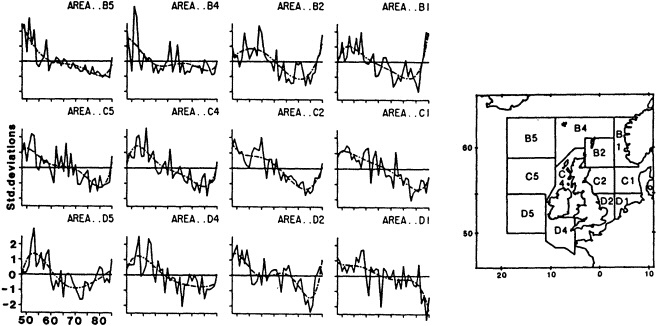
Figure 1
Trends of zooplankton abundance in 12 CPR Standard Areas (see map) around the British Isles since 1948.
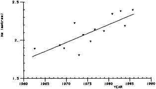
Increase in significant wave height (Hs) from ship-borne wave recorder data at the Seven Stones Lightvessel (50°N, 6°W) between 1962 and 1986. (From Bacon and Carter, 1991; reprinted with the permission of the Royal Meteorological Society.)
Andy Bakun is also showing something similar in ship observations off Spain. However, Hammond has published a measure of U.K. windiness that goes quite the other way. I do not believe that these things are irreconcilable, but they do show that looking for more and more evidence may turn up something contradictory.
But the final point I should like to make is one that Dr. McGowan and I agree on: Long-term monitoring of large numbers of biological components will eventually yield "system" and understanding. Figure 3 shows that we have for the first time an indication that the long trend in the plankton, which we think is associated with wind speed, is actually apparent in four different trophic levels in the northeast Atlantic: phytoplankton; zoöplankton (the same trend you saw before); herring; and the lay date, clutch size, and chick survival of the kittiwake, our only true marine gull. It would be a terrible shame if we went on monitoring climate and the environment without knowing about the changes going on underneath the sea surface.
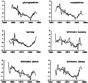
Figure 3
Standardized (zero mean, unit variance) time series and 5-year running means for abundances of phytoplankton, zoöplankton, and herring, for kittiwake laying date, clutch size and chick production, and for frequency of westerly weather, from 1955 to 1987. Ordinates in standard deviation units. In absolute terms, 5-year running means for frequency of westerly weather ranged from 60 to 82 days per year, corresponding to a maximum decrease of 27 percent.
Discussion
KUSHNIR: I'd like to add to John's comment about the recent increase in storminess in the North Atlantic. This figure is a different version of Bob's Figure 3. Here you can see the differences between the 15 warm years in the North Atlantic, 1950 to 1964, and the 15 cold years, 1970 to 1984, for both SST and sea-level pressure and winds. In the atmosphere the change from warm to cold conditions corresponded to an increase in sea-level pressure in the central North Atlantic and a decrease north of Iceland—which in turn means an increase in the strength of the westerlies, and hence also storminess, north of about 50° N.
REIFSNYDER: Let me second what John just said about the daunting complexity of systems. Many of the ecosystem models, or even just predator/prey relationships, are predicated on a stable climate. As we recognize that climate is not stable, we call into question even more than usual the predictive value of ecosystem models. We have very little hard information on climate and microclimate effects to feed into what is already something of a black-box approach.
MCGOWAN: I agree. I'm convinced that the only way we can understand how climatic variability—both magnitude and frequency—affects ecosystems is to do lots of monitoring. The reductionist studies some biologists have done are useless for prediction.
TALLEY: Bob Dickson showed some correlation of cod and haddock with events. Have you found catch data useful, John?
MCGOWAN: Not really. They correlate well with events for a few species, but mostly they don't seem to correlate with climate, or even each other. Garrod and Colebrook (1978) and other teams did a massive multi-species cross-correlation of recruitment to the North Atlantic fishery—that's the number of young fish entering per unit of time—and found a vast number of non-significant correlations. If climate is affecting the ecosystems, most of the commercially harvested fish just aren't responding. On the other hand, phytoplankton and zooplankton from those same areas track low-frequency climatic events very well.
DICKSON: Plankton data can be extremely useful in telling you which seas are dominated by eutrophication and which by climate.
RIND: John, would you care to comment on land ecosystem models? How about the agricultural ones?
MCGOWAN: Well, models for managed monocultures do rather well at predicting. They have a great deal of observational and experimental data to work with. But when you start talking about an entire complex of wild stocks, or about ecosystems, you have some complex dynamics.
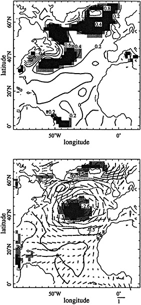
Figure 1
The difference between the average wintertime (December-April) conditions during the interval 1950 to 1964 and average wintertime conditions during the interval 1970 to 1984. Upper panel: sea-surface temperature distribution. Contour interval is 0.2°C, negative contours are dashed. Bottom panel: sea-level pressure (contours) and winds (arrows). Contour interval is 0.5 mb; arrow scale is shown at the bottom. Distribution of the t-variable corresponds to sea-surface temperature; sea-level pressure differences are denoted by three levels of gray: light for 2-2.5, medium for 2.5-3, and dark for 3-3.5. (From Kushnir, 1994; reprinted with permission of the American Meteorological Society.)
Maximum Rates of Projected and Actual Increases in Global Mean Temperature as Compared with Bioclimatic Fluctuations
WILLIAM E. REIFSNYDER1
ABSTRACT
Predictions have been made and promulgated by authoritative world bodies that the rate of model-predicted global climate warming will be 10 to 40 times that observed following the end of the last ice age (IPCC, 1990b; Schneider, 1989). If this rate of global warming were to actually occur, the effects on earth ecosystems could be dramatic, perhaps catastrophic.
A survey of published rates of increase in global mean temperature for various periods of rapid warming during the past 850,000 years shows that there appears to be an upper limit represented by the relationship ΔT = 0.38 Δy0.27, where Δy is the period during which ΔT shows sustained warming.
Analysis shows that the actual rate of warming during the millennium marking the end of the last ice age was approximately 2.5°C. Furthermore, the IPCC-I "most likely" model-estimated rate of global temperature increase in the past century (IPCC, 1990b) is 2 to 3 times the observed rate for the same period. My analysis shows that for a predicted "business-as-usual" emissions scenario, the climate change that can be expected by the end of the next century is at most twice the maximum rates observed since the last ice age. But since the models used by IPCC appear to over-predict global climate change for the past century by a factor of at least 2, one can assume that in actuality the rate of global warming over the next century will be no more than past maximum rates.
Last, contemporary measured temporal and spatial variations of climate and microclimate are shown to be several orders of magnitude greater than the secular increase of temperature predicted to result from anthropogenic global warming. This relationship may have important consequences for prediction of ecological change in the next century.
INTRODUCTION
It is supposed, and oft stated, that the increase in the rate of global warming due to anthropogenic influences may be so great that terrestrial ecosystems will not be able to adapt, and catastrophic change or collapse will ensue. The IPCC impacts assessment group stated (IPCC, 1990b):
Such warming would not only be greater than recent natural fluctuation, but it would occur 15 to 40 times faster than past natural changes. Such a rate of change may exceed the ability of many species to adapt or disperse into more favorable regions and many plant and animal species may become extinct.
This statement was based on Schneider (1989), which states that the global warming typically projected is "10 to 60 times as fast as the natural average rate of temperature change that occurred from the end of the last Ice Age to the present warm period (that is, 2°C to 6°C warming in a century from human activities compared to an average natural warming of 1°C to 2°C per millennium from the waning of the Ice Age to establishment of the present interglacial epoch)."2
Ecologists and foresters are properly concerned that the predicted changes might produce catastrophic ecological disruption. In this context, it is appropriate to examine the climatic record to determine the magnitudes of past climatic fluctuations, in particular, temperature variability on various time and space scales. Since our object of concern is ecological systems, we need to find what conditions plants and animals have been exposed to in the course of their existence. This will not tell us how any particular plant, species, or ecosystem will respond, but it will provide a useful background against which we can assess or predict response to global warming.
The objectives of the analysis below are threefold: (1) to analyze records of past climates in order to determine actual rates of warming so these rates can be compared with model predictions; (2) to investigate the variability of climate and microclimate on time scales ranging from a few minutes to a half-year; and (3) to take a brief look at the spatial variation of microclimates—the climate that plants actually live in—over space scales ranging from a meter or so to about one kilometer. I will concentrate on temperature, even though it is only one of many factors affecting plant behavior, because it is the most readily available type of observational data.
RATES OF INCREASE OF GLOBAL MEAN TEMPERATURE
Climatic modeling has emphasized global mean temperature and its generalized latitudinal variation (IPCC, 1990a; hereinafter referred to as IPCC-I). Similarly, I intend to focus on global mean temperature, with only a cursory examination of the Northern Hemisphere and the temperate latitudes, even though according to IPCC-I "land surfaces warm more rapidly than the ocean, and high northern latitudes warm more than the global mean in winter."
Only in the past 150 years or so have the instrumental observations of temperature been sufficiently good to permit the calculation of global means. Nevertheless, there are many surrogate, or proxy, observations that may be suitable for estimating global mean temperatures prior to the era of instrumental observations. While there are many uncertainties as to their applicability, such surrogate observations have been widely used for that purpose (see, for example, Chapter 7 in IPCC-I). Since most of the concern over global temperature increase appears to relate to the rate of increase rather than to absolute magnitude, I will examine records of historical climate for examples of such rates, and attempt to clarify the related uncertainties.
The IPCC Scientific Assessment Panel (IPCC-I) has made an evaluation of global temperature since 1861. For the period from 1861 to 1989, they relied on the data of Jones (1988), which show a value of 0.45°C per hundred years, or 0.58°C for the 128 years of record. Given the scantiness of the earlier observations, a more reliable estimate might be made using data from 1881 to date. Such an analysis yields a value of 0.53°C per century, or 0.57°C for the 108 years of record (see Figure 1). (Note that the abscissa is for the appropriate time interval, Δy, not for time from the present.) Since my investigation spans several orders of magnitude in the time scales and temperature scales, it is appropriate to plot the data on a log/log scale.
Balling (1992), using data limited to a more recent interval, has calculated a linearized increase in global mean temperature of 0.45°C, slightly less than the 0.53°C of the IPCC-I report. Using the relationship between the global-temperature anomalies of Jones et al. (1986) and a stratospheric dust index (estimated from solar radiation records from a high-elevation station in Austria; see Wu et al., 1990), Balling estimated the effect of dust loading on global temperature. He found that one-third of the global-temperature trend of the past 100 years disappeared, bringing that portion of the global-temperature rise that might be attributed to atmospheric carbon dioxide increase to about 0.30°C. Although it is perhaps not directly comparable, Wu et al. (1990) have estimated the increase in global night marine air temperature to be 0.49°C for the period 18561988, and 0.29°C for the period 1888-1988. When the variability caused by two additional factors, solar irradiance
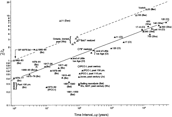
Figure 1
Rates of global warming during periods of most rapid warming in the geologic past, gleaned from various sources. Filled triangles represent global mean temperatures as inferred from measurement data. Open triangles indicate north temperate zone measurements. Open circles represent modeled or predicted values. Numbers near each point indicate the period of warming (past century) or thousands of years before present (prior to the past century) when the period of warming began. Letters in parentheses indicate source of data: Balling, 1992; Barnola et al., 1987; Boden et al., 1992; Clark, 1982; IPCC, 1990a,b; Shackleton and Opdyke, 1973; Wu et al., 1990. Solid line marks approximate upper limit of the periods of rapid global warming. Broken line indicates approximate upper limit of warming in the north temperate zone.
and the Southern Oscillation Index, is removed, the increase in global marine air temperature attributable to CO2 increase is reduced to 0.24°C.
How does this recent global temperature change compare with changes found in other periods in the geological past during which temperatures have increased rather more than the average? I have searched historical records for maximum rates of warming for various periods of time.3 From these I have selected periods during which there was sustained warming, and have calculated a warming rate for each. Data from these periods of maximum rates of warming are plotted on Figure 1 as filled triangles. They include the sharp 60-year recovery from the Little Ice Age; the 1.5°C increase over the 250 years at the end of the Little Ice Age; and the average for the 17,000 years since the start of warming at the end of the last glaciation. For comparison, I show several periods of rapid warming in the past century or so, including the largest year-to-year increases.
Shackleton and Opdyke (1973; quoted in Balling, 1992) used oxygen-isotope data from deep-sea cores as a reflection of global ice-volume changes. The ice-volume change can be interpreted in terms of global mean temperature changes over the past 850,000 years. Temperature increases for the periods that show the most rapid warming (interpreted from Balling, 1992, Figure 1) have also been plotted on Figure 1. In all of these cases, I have chosen those periods exhibiting the most rapid temperature increases.
There appears to be an upper bound to these data, represented by the straight line on the plot. The only ''outliers" are the Vostok ice-core points and a group of points representing recent ground-surface temperatures inferred from borehole temperatures in Ontario, Canada (Wang and Lewis, 1992).4 The line (fitted by eye) represents a decrease of the time-rate of warming in the form of a power law, ΔT = 0.38 Δy0.27, where 0.38 is the value of the function at Δy = 1 year. I propose that this represents the maximum rate of increase of global mean temperature observed over the past 850,000 years, no matter what the cause, or whether it arises from internal or external forcings. It seems appropriate to use this function as the standard against which we should compare model predictions of rates of global temperature increase.
Also plotted on Figure 1 (as open triangles) are several points representing Northern Hemisphere or northern temperate-zone temperature increases. These include the data of Angell (Boden et al., 1992) for the 30°-60°N latitude zone; Ontario (Canada) borehole temperatures (Wang and Lewis, 1992)5; and information from the Vostok ice cores (Barnola et al., 1987). From the Vostok data, I have chosen the two periods of most sustained and rapid warming and calculated the temperature difference for those periods.
For these data, I have drawn an upper-limit curve parallel to the global curve, a reasonable first guess.6 The equation for this line is ΔT = 1.05 Δy0.27. As expected, mid-latitude temperature increases are greater than global increases. The upper curve indicates rates of increase about 2.75 times the global curve. Also, the rates of increase in Northern Hemisphere temperature are only slightly greater (about 10 percent) than the whole-globe rates.
The first thing to note on this graph is that the "maximum" observed global rate of increase is greater by a factor of 2 or 3 than the temperature increases observed in the past century. Why should this be so? If greenhouse-gas increases over the past century (estimated to be an increase of 50 percent in the equivalent CO2 concentration (IPCC, 1990a)) have resulted in global warming, we might expect the rates of increase in global mean temperature to be at or above the "maximum" rate indicated by the solid line in Figure 1. The fact that they are well below this line implies that there may be some unknown climatic mechanism partially compensating for any warming caused by increases in greenhouse gases, or even that the observed warming is a natural trend reflecting little or none of the increase in greenhouse gases.
Another possibility is that model predictions of the effect of past increases of greenhouses gases are too high. It is thus appropriate to compare model-projected rates of increase for the past century with the observational record.
COMPARISON WITH MODEL PROJECTIONS
IPCC-I modeled the past century's observed climate, using observed increases in greenhouse gases, for various "climate sensitivities" (Figure 2). Their "best estimate" is a global mean temperature increase of 0.73°C (plotted on Figure 1 as the lowest open circle). Since the observed increase has been only 0.45°C, or even less if one accepts Balling's (1992) reanalysis, the IPCC-I model predictions are high by at least 60 percent, and perhaps as much as 150 percent.
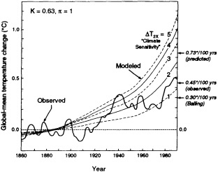
Figure 2
Global mean temperature change for the past century as modeled by IPCC-1, for various values of climate sensitivity (temperature change for a doubling of greenhouse gases) and the recommended ocean thermal diffusivity (K) and downwelling parameter (π). Observed global mean temperature is superimposed on the modeled curves. (Adapted from IPCC, 1990a, Figure 8.1a; reprinted with permission of the Intergovernmental Panel on Climate Change.)
|
4 |
Kirk Bryan (personal communication, 1992) has suggested that there are two spectral regimes in the temperature record, one for the ice age with relatively large oscillations, and another, relatively calmer, for the last 8,000 years, in which oscillations have been less rapid. However, it is likely that the physical causes limiting the rate of temperature rise would be the same during both periods; only the magnitudes of the temperature changes would be expected to be different in the two periods. |
|
5 |
The average ground-surface temperature was inferred from the temperature profile in the boreholes and the thermal conductivity of the subsurface material. This inferred temperature increase over the past century is much greater than the measured increase in global temperature, perhaps because the rate of increase is larger at high latitudes than at low latitudes. The borehole data could (and should) be checked against standard meteorological observations from nearby weather stations. I scaled the data off rather small, perhaps not perfectly accurate, diagrams. |
|
6 |
I have ignored one outlier, the temperature increase marking the end of the Younger Dryas as inferred from Greenland ice cores by Dansgaard, et al. (1989). This point implies a rate of warming twice that of the high-latitude curve of Figure 1. |
We can also compare predictions of future warming (as modeled with IPCC-I projections of increases in greenhouse gases in the next 100 years) with the "maximum" warming indicated in Figure 1. The IPCC-I business-as-usual (BaU) scenario for "realized" temperature is plotted on Figure 1 (open circle). The "realized" temperature for their ''B" scenario, representing a substantial reduction in greenhouse-gas emissions, is also plotted for comparison. If the IPCC-I model predictions are taken to be high by a factor of 2, as indicated by their overprediction of the past climate, then the predicted rates of increase in global temperature will be no greater than the observed increases over the recent geologic past. This further implies a climate sensitivity (increase in mean temperature for a doubling of greenhouse gases) closer to 1.25 than to 2.5, the value chosen by IPCC-I.7
MICROCLIMATIC REQUIREMENTS OF PLANTS
But suppose that global temperature does increase at a rate greater than that observed in the past? What effect might that have on plants and ecosystems? It is appropriate in this context to compare the variations in temperature to which plants are actually exposed and the microclimatic temperature requirements of plants.
Clearly, long-term trends in climate have been reflected in ecosystem function and species ranges, and will continue to be in the future. It is important to note, however, that insofar as the physiological response of a particular plant is climatically controlled (whether it lives or dies, flowers, reproduces, etc.), it is the local energy balance and microclimate that are controlling. Indeed, the global energy balance and climate are controlled in the first instance by the sum of local climates. Thus, it is not that global climate change influences plants and ecosystems, but the other way around: Local climates, summed over the globe, constitute global climate.
There are, of course, the questions of how, and how much, local climates are modified by changes in the global energy fluxes produced by changes in such exogenous variables as the carbon dioxide concentration of the atmosphere. It is clearly reasonable to expect the predicted changes in the surface radiation balance to result in higher surface temperatures. What is not so clear is what the time and space scales of such increases might be.
It is my contention that any secular increase in the "average" temperature of a particular location would be produced by the slow change in the energy balance concomitant with an enhanced greenhouse effect, and would appear as a superimposition on the existing climate and microclimate. It is important, therefore, to investigate the actual climatic fluctuations to which plants are exposed, in both time and space, for comparison with those likely to result from a slow secular warming. It should be noted that a warming rate of 3°C per hundred years (the BaU "realized" temperature scenario) translates to a rate of 0.03°C per year for the globe, with perhaps 2 to 3 times that rate for high latitudes. But there is little empirical evidence that such secular temperature increases will be accompanied by an increase in the variability of climatic or microclimatic temperatures (IPCC-I; NAS, 1992). An increase in the mean temperature of, say, 0.03°C might thus be expected to be accompanied by a similar increase in the mean maximum temperature. Information on the specific microclimatic requirements of various species of plants provides a perspective for assessing the significance of the changes that are expected by, for example, IPCC-I.
Information on plant species' microclimatic requirements is available in the published literature, although there is less than one might expect, given the importance of environmental conditions to the growth and survival of plants. An example of this information is presented in Figure 3, which
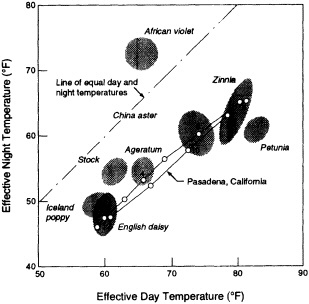
Figure 3
Optimal growing conditions for various flowers. "Effective day temperature" is the temperature during active photosynthesis; "effective night temperature" is the temperature during the dark period. Dotted circles indicate the range within which growth is optimum. Climagram for Pasadena is shown by the solid line connecting numbered months. (Source: Went, 1957, as reported in Brooks, 1958.)
shows the optimum range of day and night temperatures for flower and seed production of a number of ornamentals. Lowry (1969) provides a compendium of what is known about specific physiological requirements of plants in a microclimatic context. For example, Lowry discusses in detail the "heat units" concept, which relates the development of a plant to the thermal environment to which it is exposed. Briefly, the rate of development of a plant increases linearly with temperature above a certain threshold. It would be expected, therefore, that any increase in the temperature climate to which a plant is exposed would result in its more rapid development, other factors being equal. A relevant question in this context is what contribution a secular increase in temperature due to an augmented greenhouse effect would make to the development of a particular plant or plant association.
CLIMATIC FLUCTUATIONS ON SHORT TIME SCALES
Plants are exposed to variations in climate and microclimate that span time scales ranging from a few seconds to years or decades. They survive this variation in a number of ways, ranging from inherent flexibility and adaptation to dispersal to more favorable microclimates. It is not my purpose to create a dictionary of strategies that plants adopt. Rather, it is to look at the range of microclimates in which plants, especially, exist. In a rough way, we can compare the temperature variability of their microclimates with the increase in temperature we presume will result from an enhanced greenhouse effect. This predicted increase is of the order of 0.02°C to 0.03°C per year in the global average, and perhaps 50 percent to 100 percent greater than the global average in the high northern latitudes (IPCC-I). A location might thus experience a secular increase of 0.02°C to 0.06°C per year.
Such increases would clearly have some impact on specific plants; indeed, some would not be able to survive. Maximum microclimatic temperatures might increase to the point where a particular plant could not reproduce or would suffer fatal heat injury. An assembly of plants with similar microclimatic requirements would either die out or, alternatively, invade an area with a more suitable microclimate. It would thus be of interest to see what plants are actually exposed to in terms of climatic variability, against a background of annual increases that might be the result of global warming.
A wealth of climatic and microclimatic data is available in various compendia, notably those of Geiger (1965), Yoshino (1975), and Landsberg (1958), and in many standard texts on climatology. Data from these and other sources are plotted in Figure 4. (Again, this is a log-log plot to encompass the many orders of magnitude involved.) Data were selected not only to represent "maximum" microclimatic fluctuations, but also to be representative of various climates and microclimates. In general, these are air temperatures measured at various heights from near-surface to screen height. Unless otherwise indicated on the figure, measurements are presumed to be at heights of 1.25 to 2.0 meters above ground level, the standard specified by the World Meteorological Organization (WMO, 1983).8
The annual range of mean daily temperatures varies from about 1°C in the tropics to about 67° in the extreme continentality of Siberia. Most mid-latitude values range from about 20° to 30°. Diurnal temperature ranges are somewhat smaller. The largest I could find for an agricultural surface was about 30°, at ground level beneath an orchard. (I have ignored diurnal fluctuations on bare ground surfaces as being less relevant to plants. The greatest ground-surface diurnal range I could find was about 50°, in the Sahara (Geiger, 1965).)
Information on shorter-period fluctuations is scarce in the scientific literature; a few representative values are given in Figure 4. It is apparent that many plants and plant surfaces are subjected to short-period fluctuations on the order of 1°C to 30°C.
Does this variability have any significance for how well plants and ecosystems would survive a secular warming on the order of 0.06°C per year? My own experience leads me to believe that such warming would, in general, lead to slow ecological changes of the same order of magnitude as those that have always been a part of ecosystem behavior. In terms of human perceptibility, these changes are usually scarcely noticeable. Thus, the forest-prairie boundary may move back and forth in response to climatic change, but the rate may be measured in centimeters or meters per year. Looking back in geologic time tends to produce a foreshortened view. The thousand-year-long warming at the end of the last ice age may appear to us to have had ecological consequences more drastic than any observer on the scene at the time would have noticed.
SPACE VARIATIONS IN MICROCLIMATE
As I noted previously, a plant that is experiencing a secular change in the microclimate, slow though it may be, may find that it can no longer exist or reproduce and reestablish itself in that changed microclimate. It may be subject to ravages of disease or pests that did not exist previously. However, its reproductive processes may permit the plant to become established in a nearby microclimate that is more favorable to its survival. Indeed, this is one of the ways that species distribution changes in response to
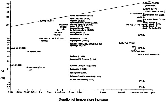
Figure 4
Temperature change as a function of time interval in various bioclimates. It is the time during which temperature at the particular location was increasing. Data sources: Brooks, 1958; Geiger, 1965; Hare and Hay, 1974; Koeppe and De Long, 1958; Landsberg, 1958; Yoshino, 1975.
climatic trends. So it is of interest to see how microclimate (and mesoclimate) varies over space.
Figure 5 presents data from a number of sources on the variations in temperature that may be found within distances ranging from a meter or so to one kilometer. Most of these are for maximum daytime temperatures, and have been chosen to illustrate typical conditions.
Large differences in temperature—on the order of 10°C to 15°C—can be found in close proximity, as on the sunny side of a small mound or furrow as compared with the opposite side. Significant but less extreme temperature differences can be found over distances ranging upwards of 10 meters. Microclimatic extremes are greater than mesoclimatic extremes. Indeed, a negative exponential decrease in the temperature differences as a function of distance between measurement locations appears in this sample.
DISCUSSION
It seems to me that this considerable variability has significance for predictions of ecological change in response to "global warming". Any long-term increase (or decrease) in the temperature to which a plant or ecosystem is exposed will have some effect. Plants in specific locations within an ecosystem may not be able to survive. But plants at unfavorable boundaries in the same ecosystem may reproduce in more favorable conditions nearby; their geographical range may thus be altered. Whether this is a "catastrophic" response depends on human definitions.9
Science (1988, 242:1010) asks, "Is there life after climate change?" and answers "Yes, but the world will be a different place, with an abundance of male alligators, migrating trees, and a plethora of parasites." It is absurd to ask what will happen after climate change; climate is changing all the time, at all possible scales of time and space. There is no before and after. Thompson Webb is quoted in this article as saying that we are moving into a new biological world. In actuality, we are forever moving into new biological worlds. The relevant question for public policy is whether the climatic changes that occur as the result of increases in greenhouse gases will have consequences that are obviously and dramatically disruptive of ecosystem behavior and human response.
We might ask ourselves whether, if we had never heard about "global warming," would we have inferred that such a process was at work, on the basis of observations of plant and animal behavior (or even the climatic record) during the past century. I contend that we could not. Long-term climatic change—from whatever cause—is masked by the
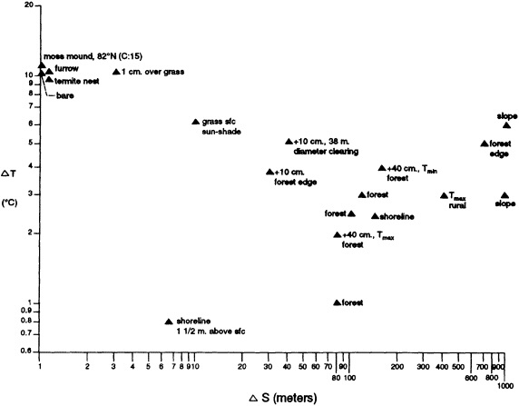
Figure 5
Variation in temperature over various distances; locations as indicated. Data sources: Corbet, 1972; Fowler, 1971; Geiger, 1965; Landsberg, 1958; Shitara, 1971; Yoshino, 1975.
shorter-term fluctuations, which are several orders of magnitude greater. It is difficult to see how such long-term secular changes could be catastrophic to the world's biological systems.
This view is consistent with the "final words" of the Panel on Policy Implications of Greenhouse Warming of the National Academy of Sciences (NAS/NAE/IOM, 1992):
So far as we can reason from the assumed gradual changes in climate, their impacts will be no more severe, and adapting to them will be no more difficult, than for the range of climates already on earth and no more difficult than for other changes humanity faces. However, because we cannot rule out major changes in ocean currents, atmospheric circulations, or other natural or social surprises, we need to be alert to any substantial probability or signs of such changes that would require responses not considered in our report.
From a scientific point of view, long-term changes and interconnections are of great interest and worthy of continued attention. For many users of climatic information, however, predictions of short-term climate would be of more value than predictions of the slow secular changes expected to result form anthropogenic greenhouse-gas increases or of likely average conditions for the end of the next century. For example, farmers would find an accurate forecast of the next growing season's climate to be very valuable, but a forecast of a slow climate trend even over the next decade would be of marginal value to them. Foresters are in a similar situation. Despite the long life of a tree or a forest ecosystem, most forest-management decisions consider a time frame of less than ten years.
Now it may be, as many have argued, that it will never be possible for modelers to predict the next year's climate, or even the next decade's, because of the inherent randomness of climatic processes. But where do endogenous variables end and exogenous variables take over? What is the scale of ultimate believability of climatic forecasts? Decades? Centuries? Millennia? This is not a trivial question. Furthermore, as I have argued elsewhere (Reifsnyder, 1989), society must always make important decisions in the face of climatic uncertainty. We may plan for global warming, but there is always some non-zero chance that we will be faced with global cooling instead.
SUMMARY AND CONCLUSIONS
My findings are these:
-
There is a well-defined limit to temporal rates of increase in global mean temperature for periods of warming during the past 850,000 years. It can be expressed in the relationship ΔT = 0.38 Δy0.27, where Δy is the number of years during which sustained warming has occurred.
-
Natural fluctuations of climate are several orders of magnitude larger than both the secular increase of temperature predicted by current climate models and the probable actual increase over the next century.
-
The results of comparisons of predicted rates of global temperature increase with past observed rates of increase depend greatly on the time periods chosen. Unless the time periods are carefully selected to represent comparable periods (of rapid warming, for example), comparisons can be so skewed as to be misleading or meaningless. Even if the IPCC-1 model predictions were correct, the rate of global temperature increase over the next century would probably be no more than the maximum rates of increase experienced at various times in the past 8,000 years. At worst, they would be double those rates. Even these predicted increases in temperature will be so small by comparison with natural climatic fluctuations, and spread over such a long time scale, that their short-term impact on human behavior and welfare is likely to be minimal and probably not measurable. It thus seems reasonable to conclude that the long-term secular temperature change will not produce dramatic and disruptive changes in the earth's biological systems.
Does this mean that we as scientists should not be interested in the scientific issues entailed by enhanced greenhouse effects and their potential impacts? Not at all: What happens to the earth's climate because of human activities, and what happens to the earth's ecosystems as a result, should be foci of intense scientific scrutiny. We have only one earth to lose, and we should not lose it by default. Let us put our effort into devising productive research approaches, not waste it in chasing chimeras.
Commentary on the Paper of Reifsnyder
SOROOSH SOROOSHIAN
University of Arizona
In his analysis, Dr. Reifsnyder has used temperature as the sole indicator of climate variability, in both space and time. I should like to bring up two points related to this approach.
First, the data Dr. Reifsnyder has used in his analysis come from the published literature and from analyses made by numerous researchers. Some of them are instrumental observations; others result from the analysis of proxy records. They come from many sources, various time periods, and locations worldwide. Not only does each type carry an individual potential for error, but combining them may risk an apples-and-oranges comparison. When data from varied sources are used, as Dr. Reifsnyder and some others have done, one must ask, "To what extent do such uncertainties affect the results and the conclusions drawn from them?"
Even if we ignore the temporal and spatial uncertainties associated with the temperature data, data can still be biased because of changes in instrument technology or in the manner in which measurements are taken. A fair degree of confidence can be placed in data that have been corrected for sources of error; when we are talking about deducing several degrees of temperature change over hundreds or thousands of years from proxy records, we need to acknowledge the magnitude of the associated uncertainties. Let me adduce a similar situation with precipitation data. In collaboration with the Agricultural Research Service, we at Arizona have been monitoring precipitation amounts over a small, well-instrumented experimental watershed. We have a very high density of sophisticated rain gauges, yet the analysis of our data shows that if the measurement errors are not taken into account, the information value may be limited. Conclusions drawn from those data need to be questioned as well.
Dr. Reifsnyder's paper also deals with the impact of temperature change on vegetation. I will not take issue with his position that vegetation will have the ability to tolerate the changes in global mean temperature estimated by various models. I will, however, argue that not only temperature is involved. Even small changes in mean global temperature can have an impact on the general circulation of the atmosphere and the oceans. A temperature change not only might increase the severity of droughts and floods but might expand the regions of the globe affected by them as well. Trees might tolerate a temperature change, but could they also survive a sustained drought?
I should like to endorse a third point that Dr. Reifsnyder makes, although indirectly: Scientists need to be responsible
in conveying the results of their studies to decision- and policy-makers. The use of data with a high degree of uncertainty, or the results of models based on questionable assumptions, places the credibility of our science at risk.
Discussion
RIND: I find myself in the strange position of having to defend Steve Schneider. I'm not sure it's reasonable to compare the glacial-to-interglacial warming over 5000 years with the projected warming over the next 100 years or so, when the time spans are so different.
REIFSNYDER: Oh, I admit that's comparing apples with oranges. If you extrapolate the IPCC values for 1000 years they become absurd. You do have to be careful how you choose the periods for comparison. The longer the time period, the slower the rate of change.
MOREL: Allow me in turn to defend the IPCC report. For a U.N.-sponsored six-month exercise, I would say it's remarkably respect-worthy. We were trying to give the reader a reasonable idea of what could happen, working from uncertainties quite as large as one finds in nature. After all, we can't even link some substantial ecosystem changes, such as the desertification in Africa, with any changes in global climate indicators.
REIFSNYDER: I quite agree. However, that report has been used by non-scientific people as the basis for so many outrageous suggestions that I think it's important to call attention to its inconsistencies and limitations.
LEHMAN: I hesitate to add fuel to the fire, but we did find that during the deglaciation sea-surface temperatures in the North Atlantic changed by as much as 5°C in less than 40 years, in both negative and positive directions. Ice cores show warming of 7° in 50 years. These regional modulations probably relate to some fairly significant global changes.
TRENBERTH: It seems to me that the models essentially represent the anthropogenic change. Why should they be relevant to natural climate change? Conversely, how can one deduce the rate at which man can change the climate from that of natural change?
REIFSNYDER: My point was more a matter of what plants have been exposed to, whatever the origin of the change. The slow secular temperature increase ascribable to increased carbon dioxide in the atmosphere is several orders of magnitude less than that of the climate to which a plant is exposed in the course of its life.
JONES: I think we should keep in mind that most of the points to the right of the 100-year band on your Figure 1 are regional. A 10°C change in Vostok, or even the entire Antarctic region, probably means a global change on the order of 4° or 5°. Also, I'd like to emphasize that small changes can make a significant difference. In the 1920s and 1930s there were some very warm summers in northern Scandinavia, meaning 1° or 2°C warmer on average. As a result, the tree line moved many kilometers further north in a short space of time.
REIFSNYDER: That's not what's at issue. My question is how much an increase due to global warming will affect such natural changes.
GROISMAN: I'd just like to add another reminder that the rate of mean temperature changes at high latitudes is not the same as the global rate, either in the last hundred years' observations or in the model results, whatever the IPCC report may say.
KEELING: I think this is just the kind of healthy challenge the IPCC report needs to counter the word-bite publicity it's been getting. I'd like to make a few points here. First, I don't see how we can be sure that the reason for the temperature increase you cited is global warming. Even worse, it may be that there are several anthropogenic signals whose effects are partially canceling each other out; Mike Schlesinger brought that possibility up at a recent meeting.
Second, those fluxes bother me. The fluxes involved in the CO2 increase over the last 100 years are dwarfed by the natural fluxes in the carbon cycle, and I don't think they have anything to do with the accumulation of CO2 in the atmosphere. Third, I don't think we need to worry so much about what level of temperature we reach as about how long the increased temperature will persist. Some trees can handle a passing fire; that doesn't mean they could survive 5 years of heat and drought, followed by another 5. That sort of possible anthropogenic effect is what we need to know about.
REIFSNYDER: Indeed. But in response to your first point, let me say that we really have no better hypothesis then a CO2 increase for what caused the warming over the last 100 years. My position is that it's our best estimate.
GROOTES: A propose of climate's societal impacts, let us not forget the Norse colonies in Greenland. They lived there happily for 500 years before being driven out by the effects of the Little Ice Age. But I have a question for you, Bill. I understood you to say that the concern about global warming should and probably would disappear, and we should concentrate our efforts elsewhere. What are your suggestions?
REIFSNYDER: Oh, there's a great deal more we need to know about anthropogenic global warming. I just think it will die down as a social-policy issue, since we can't yet relate it to the warming during this century. As for Greenland. remember that the Little
Ice Age temperature changes were significantly more severe than the 0.02° or 0.04°C per year that presumably can be attributed to anthropogenic carbon dioxide.
PERRY: You seem to be advancing a new biological principle here: Changes in the mean state over long periods are insignificant as long as they are small in relation to the total range of conditions experienced by the individual organism. Surely you don't mean you would be happy if the temperatures you survived on your drive here from New Mexico became your long-term environment?
REIFSNYDER: No, that would certainly qualify as a profound change to my local ecosystem. But my point, really, is that the changes we have seen on the scale of a lifetime cannot be ascribed to anthropogenic global warming.
KARL: I'd like to raise a question related to your Figure 1, Bill, that I think we should be considering at this workshop: Can you get by with a much smaller spatial resolution as the time interval increases with respect to the time frame you're dealing with? Can you get away with not having a complete global average if you're dealing with 1000 years instead of 10,000?
MCGOWAN: Very few ecologists I know of have ever thought that the effects of temperature per se on photosynthesis or animal behavior were the issue. For instance, the California Current, which is very heterogeneous in both space and time, has lots of 2°C variations on many time scales. Despite this exposure to temperature shifts, when the mean temperature of the upper 100 meters of the Current rose a little less than 2° during the 1958 and 1983 El Niños, the effects on both plants and animals were catastrophic. Of course it wasn't just the temperature, which I think is a rather poor proxy measurement of what's really happening; it was the fact that the mixed layer collapsed. There were no nutrients coming in, there was advective movement of boundaries, and so on.
REIFSNYDER: Temperature just happens to be the one thing we have data on, and I think it may be important as a proxy for other variations. Certainly ecosystems respond to all kinds of things, often catastrophically. It seems to me that your example demonstrates my point that it's these short-term excursions from the mean, which as far as we know are normal climate behavior, that produce catastrophic ecosystem changes, not the warming of 0.05°C or less per year ascribable to anthropogenic CO2.
Proxy Indicators of Climate Reference List
Aagaard, K., J.H. Swift, and E.C. Carmack. 1985. Thermohaline circulation in the Arctic Mediterranean seas. J. Geophys. Res. 90(C3):4833-4846.
Aebischer, N.J., J.C. Coulson, and J.M. Colebrook. 1990. Parallel long-term trends across four marine trophic levels and weather. Nature 347:753-755.
Aharon, P. 1985. Carbon isotope record of late Quaternary coral reefs: Possible index of sea surface paleoproductivity. In The Carbon Cycle and Atmospheric CO2: Natural Variations Archean to Present. E.T. Sundquist and W.S. Broecker (eds.). Geophysical Monograph 32, American Geophysical Union, Washington, D.C., pp. 343-355.
Allan, R.J., N. Nicholls, P.D. Jones, and I.J. Butterworth. 1991. A further extension of the Tahiti-Darwin SOI, early ENSO events and Darwin pressure. J. Climate 4:743-749.
Allen, W.E. 1941. Twenty years' statistical studies of marine plankton dinoflagellates off southern California. Amer. Mid. Nat. 26:603-635.
Alley, R.B., P.M. Grootes, D. Meese, A.J. Gow, K. Taylor, and K.M. Cuffey. 1991. Climate at the Greenland Summit: Little Ice Age to modern. EOS 72:66.
Alley, R.B., D.A. Meese, C.A. Shuman, A.J. Gow, K.C. Taylor, P.M. Grootes, J.W.C. White, M. Ram, E.D. Waddington, P.A. Mayewski, and G.A. Zielinski. 1993. Abrupt increase in Greenland snow accumulation at the end of the Younger Dryas event. Nature 362:527-529.
Ammann, B., and A.F. Lotter. 1989. Late glacial radiocarbon- and palynostratigraphy on the Swiss Plateau. Boreas 18:109-126.
Atkinson, T.C., K.R. Briffa, and G.R. Coope. 1987. Seasonal temperatures in Britain during the past 22,000 years, reconstructed using beetle remains. Nature 325:587-592.
Bacon, S., and D.J.T. Carter. 1991. Wave climate changes in the North Atlantic and North Sea. Int. J. Climatol. 11:545-558.
Bacon, S., and D.J.T. Carter. 1993. A connection between mean wave height and atmospheric pressure gradient in the North Atlantic. Int. J. Climatol. 13:423-436.
Bainbridge, A. (ed.). 1981. GEOSECS Atlantic Expedition Hydrographic Data. Vol. 1. U.S. Government Printing Office, Washington, D.C.
Balling, R.C., Jr. 1992. The Heated Debate: Greenhouse Predictions versus Climate Reality. Pacific Research Institute for Public Policy, San Francisco.
Bard, E., M. Arnold, P. Maurice, J. Duprat, J. Moyes, and J.-C. Duplessy. 1987. Retreat velocity of the North Atlantic polar front during the last deglaciation determined by 14C accelerator mass spectrometry. Nature 328:791-794.
Bard, E., B. Hamelin, R.G. Fairbanks, and A. Zindler. 1990. Calibration of the 14-C time-scale over the past 30,000 years using mass spectrometric U-Th ages from Barbados corals. Nature 345:405-410.
Barnes, D.J., and J.M. Lough. 1989. The nature of skeletal density banding in scleractinian corals: Fine banding and seasonal patterns. J. Exp. Mar. Bio. 126:119-134.
Barnett, T.P. 1991. The interaction of multiple time scales in the tropical climate system. J. Climate 4:269-285.
Barnett, T.P., and M.E. Schlesinger. 1987. Detecting changes in global climate induced by greenhouse gases. J. Geophys. Res. 92:14772-14780.
Barnola, J.M., D. Raynaud, Y.S. Korotkevich, and C. Lorius. 1987. Vostok ice core provides 160,000-year record of atmospheric CO2. Nature 329:408-414.
Barnola, J.M., P. Pimienta, D. Raynaud, and Y.S. Korotkevich. 1991. CO2-climate relationship as deduced from the Vostok ice core: A re-examination based on new measurements and on a re-evaluation of the air dating. Tellus 43B:83-90.
Barry, R.G. 1978. Climate fluctuations during the periods of historical and instrumental record. In Climatic Change and Variability: A Southern Hemisphere Perspective. A.B. Pittock, L.A. Frakes,
D. Jenssen, J.A. Peterson, and J.W. Zillman (eds.). Cambridge University Press, London, pp. 150-166.
Barry, R.G., and R.J. Chorley. 1982. Atmosphere, Weather, and Climate (6th ed.). Routledge, New York, 387 pp.
Baumgartner, T.R., A. Soutar, and V. Ferreira-Bartrina. 1992. Reconstruction of the history of Pacific sardine and northern anchovy populations over the past two millennia from sediments of the Santa Barbara Basin, California. Calif. Coop. Oceanic Fisheries Invest. Rpts. 33:24-40.
Bé, A.W.H., and D.S. Tolderlund. 1971. Distribution and ecology of living planktonic foraminifera in surface waters of the Atlantic and Indian oceans. In Micropaleontology of Oceans. B.M. Funnell and W.R. Riedel (eds.). Cambridge University Press, London, pp. 105-149.
Beadle, L.C. 1974. The Inland Waters of Tropical Africa: An Introduction to African Limnology. Longman, London.
Beck, J.W., R.L. Edwards, E. Ito, F.W. Taylor, J. Recy, F. Rougerie, P. Joannot, and C. Henin. 1992. Sea-surface temperature from coral skeletal strontium/calcium ratios. Science 257:644-647.
Bender, M., T. Sowers, M.-L. Dickson, J. Orchardo, P. Grootes, P.A. Mayewski, and D.A. Meese. 1994. Climate correlations between Greenland and Antarctica during the past 100,000 years. Nature 372: 663-666.
Berger, A.L. 1978. Long-term variations of daily insolation and Quaternary climate changes. J. Atmos. Sci. 35:2362-2367.
Bergthorsson, P. 1969. An estimate of drift ice and temperature in Iceland in 1000 years. Jokull 19:94-101.
Bernal, P.A., and J.A. McGowan. 1981. Advection and upwelling in the California Current. In Coastal Upwelling. F.A. Richards (ed.). American Geophysical Union, Washington, D.C., pp. 381-399.
Boden, T.A., R.J. Sepanski, and F.W. Stoss (eds.). 1992. Trends '91: A Compendium of Data on Global Change. Publ. No. ORNL/CDIAC-49, Carbon Dioxide Information Analysis Center, Oak Ridge National Laboratory, Tennessee.
Bottomley, M., C.K. Folland, J. Hsiung, R.E. Newell, and D.E. Parker. 1990. Global Ocean Surface Temperature Atlas (GOSTA). H.M.S.O., London, 20 pp., 313 plates.
Boutron, C. 1980. Respective influence of global pollution and volcanic eruptions on the past variations of the trace metals content of Antarctic snows since 1880s. J. Geophys. Res. 85:7426-7432.
Boyle, E.A. 1988. Cadmium: Chemical tracer of deepwater paleoceanography. Paleoceanography 3:471-489.
Boyle, E.A., and L. Keigwin. 1987. North Atlantic thermohaline circulation during the past 20,000 years linked to high-latitude surface temperature. Nature 330:35-40.
Boyle, E.A., F. Sclater, and J.M. Edmond. 1976. On the marine geochemistry of cadmium. Nature 263:42-44.
Bradley, R.S. 1985. Quaternary Paleoclimatology: Methods of Paleoclimatic Reconstruction. Allen and Unwin, London and Boston, 472 pp.
Bradley, R.S. 1988. The explosive volcanic eruption signal in northern hemisphere continental temperature records. Climatic Change 12:221-243.
Bradley, R.S., and J.A. Eddy. 1989. Records of past global changes. In Global Changes of the Past. R.S. Bradley (ed.). UCAR/Office for Interdisciplinary Earth Studies, Boulder, Colorado, pp. 5-9.
Bradley, R.S., and J.K. Eischeid. 1985. Aspects of the precipitation climatology of the Canadian high Arctic. In Glacial, Geologic and Glacio-Climatic Studies in the Canadian High Arctic. R.S. Bradley (ed.). Dept. of Geology and Geography, University of Massachusetts at Amherst, pp. 250-271.
Bradley, R.S., and P.D. Jones (eds.). 1992. Climate Since A.D. 1500. Routledge, New York, 679 pp.
Bradley, R.S., P.M. Kelly, P.D. Jones, C.M. Goodess, and H.F. Diaz. 1985. A Climatic Data Bank for Northern Hemisphere Land Areas, 1851-1980. Technical Report TR017, U.S. Dept. of Energy, Carbon Dioxide Research Division, 335 pp.
Bradley, R.S., H.F. Diaz, J.K. Eischeid, P.D. Jones, P.M. Kelly, and C.M. Goodess. 1987a. Precipitation fluctuations over northern hemisphere land areas since the mid-19th century. Science 237:171-175.
Bradley, R.S., H.F. Diaz, G. Kiladis, and J.K. Eischeid. 1987b. ENSO signal in continental temperature and precipitation records. Nature 327:497-501.
Brassel, S.C., G. Eglinton, I.T. Marlowe, U. Pflaumann, and M. Sarnthein. 1986. Molecular stratigraphy: A new tool for climatic assessment. Nature 320:129-133.
Briffa, K.R., and P.D. Jones. 1993. Global surface air temperature variation over the twentieth century: Part 2, Implications for large-scale palaeoclimatic studies of the Holocene. Holocene 3:82-93.
Briffa, K.R., T.S. Bartholin, D. Eckstein, P.D. Jones, W. Karlén, F.H. Schweingruber, and P. Zetterberg. 1990. A 1400-year tree-ring record of summer temperature. Nature 346:434-439.
Briffa, K.R., P.D. Jones, T.S. Bartholin, D. Eckstein, F.H. Schweingruber, W. Karlén, P. Zetterberg, and M. Eronen. 1992a. Fennoscandian summers from A.D. 5(X): Temperature changes on short and long time scales. Climate Dynamics 7:111-119.
Briffa, K.R., P.D. Jones, and F.H. Schweingruber. 1992b. Tree-ring density reconstructions of summer temperature patterns across western North America since A.D. 1600. J. Climate 5:735-754.
Briffa, K.R., P.D. Jones, F.H. Schweingruber, S.G. Shiyatov, and E.R. Cook. 1995. Unusual twentieth-century summer warmth in a 1,000-year temperature record from Siberia. Nature 376:156-159.
Broecker, W.S. 1987. Unpleasant surprises in the greenhouse? Nature 328:123-126.
Broecker, W.S. 1991a. The great ocean conveyor. Oceanography 4:79-89.
Broecker, W.S. 1991b. Strength of the Nordic heat pump. In The Last Deglaciation: Absolute and Radiocarbon Chronologies. E. Bard and W.S. Broecker (eds.). NATO ASI Series I. Vol. 2, Springer-Verlag, pp. 173-182.
Broecker, W.S., and G.H. Denton. 1989. The role of ocean-atmosphere reorganizations in glacial cycles. Geochim. Cosmochim. Acta 53:2465-2501.
Broecker, W.S., D.M. Peteet, and D. Rind. 1985. Does the ocean-atmosphere system have more than one stable mode of operation? Nature 315:21-25.
Broecker, W.S., M. Andree, W. Wolfli, H. Oeschger, G. Bonani, J. Kennett, and D. Peteet. 1988. The chronology of the last
deglaciation: Implications for the cause of the Younger Dryas event. Paleoceanography 3:1-19.
Broecker, W.S., G. Bond, M. Klas, G. Bonani, and W. Wölfli. 1990a. A salt oscillator in the glacial Atlantic? 1. The concept. Paleoceanography 4:469-477.
Broecker, W.S., M. Klas, E. Clark, S. Trumbore, G. Bonani, W. Wolfli, and S. Ivy. 1990b. Accelerator mass spectrometric radiocarbon measurements on foraminifera shells from deep-sea cores. Radiocarbon 32:119-133.
Brooks, F.A. 1958. An Introduction to Physical Microclimatology. University of California, Davis.
Brooks, C.E.P. 1923. Variations in the Levels of the Central African Lakes, Victoria and Albert. Geophysical Memoir No. 20. U.K. Meteorological Office, London.
Bryan, F. 1986. High-latitude salinity effects and interhemisphere thermohaline circulations . Nature 323:301-304.
Budd, W.F., and V.I. Morgan. 1977. Isotopes, climate and ice sheet dynamics from core studies on Law Dome, Antarctica. IAHS No. 118:312-325.
Cane, M.A. 1983. Oceanographic events during El Niño. Science 222:1189-1195.
Carpenter, S.R., K.L. Cottingham, and D.E. Schindler. 1992. Biotic feedback in lake phosphorus cycles. Trends Ecol. Evol. 7(10):332-336.
Carriquiry, J.D., M.J. Risk, and H.P. Schwarcz. 1988. Timing and temperature record from the stable isotopes of the 1982-1983 El Niño warming event in eastern Pacific corals. Palaios 3:359-364.
Chan, L.H., D. Drummond, J.M. Edmond, and B. Grant. 1977. On the barium data from the Atlantic GEOSECS Expedition. Deep-Sea Res. 24:613-649.
Chappelaz, J., J.M. Barnola, D. Raynaud, Y.S. Korotkevich, and C. Lorius. 1990. Ice-core record of atmospheric methane over the past 160,000 years. Nature 345:127-131.
Chelton, D.B., P.A. Bernal, and J.A. McGowan. 1982. Large-scale interannual physical and biological interaction in the California Current. J. Mar. Res. 40:1095-1125.
Clark, W.C. (ed.). 1982. Carbon Dioxide Review 1982. Oxford University Press, Oxford.
Clarke, R.A., and J.C. Gascard. 1983. The formation of Labrador Sea water. Part 1: Large-scale processes. J. Phys. Oceanogr. 13:1764-1778.
CLIMAP Project Members. 1981. Seasonal reconstruction of the earth's surface during the last glacial maximum. Map and Chart Series No. MC-36, Geological Society of America, Boulder, Colo., 18 pp.
Cohen, S.J. 1986. Impacts of CO2-induced climatic change on water resources in the Great Lakes Basin. Climatic Change 8:135-153.
Cole, J.E. 1992. Interannual-Decadal Variability in Tropical Climate Systems: Stable Isotope Records and General Circulation Model Experiments. Ph.D. thesis, Columbia University.
Cole, J.E., and R.G. Fairbanks. 1990. The Southern Oscillation recorded in the oxygen isotopes of corals from Tarawa Atoll . Paleoceanography 5:669-683.
Cole, J.E., G.T. Shen, R.G. Fairbanks, and M. Moore. 1992. Coral monitors of El Niño/Southern Oscillation dynamics across the equatorial Pacific. In El Niño: Historical and Paleoclimatic Aspects of the Southern Oscillation. H. Diaz and V. Markgraf (eds.). Cambridge University Press, Cambridge, U.K., pp. 349-375.
Cole, J.E., R.G. Fairbanks, and G.T. Shen. 1993. The spectrum of recent variability in the Southern Oscillation: Results from a Tarawa Atoll coral. Science 262:1790-1793.
Cole, J.E., R.G. Fairbanks, and G.T. Shen. 1995. Monitoring the tropical ocean and atmosphere using chemical records from long-lived corals. In Natural Climate Variability on Decade-to-Century Time Scales. D.G. Martinson, K. Bryan, M. Ghil, M.M. Hall, T.R. Karl, E.S. Sarachik, S. Sorooshian, and L.D. Talley (eds.). National Academy Press, Washington, D.C.
Colebrook, J.M. 1985. Sea surface temperatures and zooplankton, North Sea 1948 to 1983. J. Cons. Int. Explor. Mer 42:179-185.
Colgan, M.W., and D. Malmquist. 1987. The Urvina Bay uplift: A dry trek through a coral community. Oceanus 30:61-66.
Colinvaux, P.A., M.C. Miller, K.-B. Liu, M. Steinitz-Kannan, and I. Frost. 1985. Discovery of permanent Amazon lakes and hydraulic disturbance in the upper Amazon Basin. Nature 313:42-45.
Conversi, A. 1992. Variability of water quality data collected near three major southern California sewage outfalls. Ph.D. dissertation. Scripps Institution of Oceanography, Univ. Calif., San Diego, 109 pp.
Conversi, A., and J.A. McGowan. 1994. Natural versus human-caused variability of water clarity in the Southern California Bight. Limnol. Oceanogr. 39(3):632-648.
Cook, E.R., K.R. Briffa, S. Shiyatov, and V. Mazepa. 1990. Tree-ring standardization and growth-trend estimation. In Methods of Dendrochronology: Applications in the Environmental Sciences. E.R. Cook and L.A. Kairiukstis (eds.). Kluwer, Dordrecht, pp. 104-123.
Cook, E., T. Bird, M. Peterson, M. Barbetti, B. Buckley, R. D'Arrigo, R. Francey, and P. Tans. 1991. Climatic change in Tasmania inferred from a 1089-year tree-ring chronology of subalpine Huon pine. Science 253:1266-1268.
Cook, E., T. Bird, M. Peterson, M. Barbetti, B. Buckley, R. D'Arrigo, and R. Francey. 1992. Climatic change over the last millennium in Tasmania reconstructed from tree rings. Holocene 2(3):205-217.
Cook, E.R., K.R. Briffa, D.M. Meko, D.A. Graybill, and G. Funkhouser. 1995a. The 'segment-length curse' in long tree-ring chronology development for paleoclimatic studies. Holocene 5:229-237.
Cook, E.R., B.M. Buckley, and R.D. D'Arrigo. 1995b. Interdecadal temperature oscillations in the Southern Hemisphere: Evidence from Tasmanian tree rings since 300 B.C. In Natural Climate Variability on Decade-to-Century Time Scales. D.G. Martinson, K. Bryan, M. Ghil, M.M. Hall, T.R. Karl, E.S. Sarachik, S. Sorooshian, and L.D. Talley (eds.). National Academy Press, Washington, D.C.
Coope, G.R. 1977. Fossil coleopteran assemblages as sensitive indicators of climatic changes during the Devensian (last) cold stage. Phil. Trans. Roy. Soc. London B 280:313-340.
Coope, G.R., and J.A. Brophy. 1972. Late glacial environmental changes indicated by a coleopteran succession from North Wales. Boreas 1:97-142.
Cooper, N.S., K.D.B. Whysall, and G.R. Bigg. 1989. Recent deca-
dal climate variations in the tropical Pacific. Int. J. Climatol. 9:221-242.
Corbet, P.S. 1972. The Microclimate of Arctic Plants and Animals, on Land and in Fresh-Water. Acta Arctica 18. 43 pp.
Coughlan, M.J. 1979. Recent variations in annual-mean maximum temperatures over Australia. Quart. J. Roy. Meteorol. Soc. 105:707-719.
CPR Survey Team. 1992. Continuous plankton records: The North Sea in the 1980s. ICES Mar. Sci. Symp. 195:243-248.
Craig, H., and C.C. Chou. 1982. Methane: The record in polar ice cores. Geophys. Res. Lett. 9:1221-1224.
Craig, H., C.C. Chou, J.A. Welhan, C.M. Stevens, and A.E. Engelkemeir. 1988a. The isotopic composition of methane in polar ice cores. Science 242:1535-1539.
Craig, H., Y. Horibe, and T. Sowers. 1988b. Gravitational separation of gases and isotopes in polar ice caps. Science 242:1675-1678.
Crowe, R.B. 1992. Extension of Toronto temperature time-series from 1840 to 1778 using various United States and other data. In The Year Without a Summer? World Climate in 1816. C.R. Harington (ed.). Canadian Museum of Nature, Ottawa, pp. 145-161.
Currie, R.G. 1981. Evidence for 18.6 year MN signal in temperature and drought conditions in North America since A.D. 1800. J. Geophys. Res. 86:11055-11064.
Curtis, J.H., and D.A. Hodell. 1993. An isotopic and trace-element study of ostracods from Lake Miragoane, Haiti: A 10,500 year record of paleosalinity and paleotemperature. In Climate Change in Continental Isotopic Records. P.K. Swart, K.C. Lohmann, J. McKenzie, and S. Savin (eds.). AGU Geophys. Monogr. 78:135-152.
Dansgaard, W., S.J. Johnsen, J. Møller, and C.C. Langway, Jr. 1969. One thousand centuries of climatic record from Camp Century on the Greenland ice sheet. Science 166:377-381.
Dansgaard, W., S.J. Johnsen, H.B. Clausen, and C.C. Langway, Jr. 1971. Climatic record revealed by the Camp Century ice core. In The Late Cenozoic Glacial Ages. K.K. Turekian (ed.). Yale University Press, pp. 37-56.
Dansgaard, W., S.J. Johnsen, H.B. Clausen, and N. Gundestrup. 1973. Stable isotope glaciology. Medd. Grønland 197:1-53.
Dansgaard, W., S.J. Johnsen, N. Reeh, N. Gundestrup, H.B. Clausen, and C.U. Hammer. 1975. Climatic changes, Norsemen and modern man. Nature 255:24-28.
Dansgaard, W., H.B. Clausen, N. Gundestrup, C.U. Hammer, S.F. Johnsen, P.M. Kristinsdottir, and N. Reeh. 1982. A new Greenland deep ice core. Science 218:1273-1277.
Dansgaard, W., S.J. Johnsen, H.B. Clausen, D. Dahl-Jensen, N. Gundestrup, C.U. Hammer, and H. Oeschger. 1984. North Atlantic climate oscillations revealed by deep Greenland ice cores. In Climate Processes and Climate Sensitivity. J.E. Hansen and T. Takahashi (eds.). Geophys. Monograph 29 (Maurice Ewing Series), American Geophysical Union, Washington, D.C., pp. 288-298.
Dansgaard, W., J.W.C. White, and S.J. Johnsen. 1989. The abrupt termination of the Younger Dryas climate event. Nature 339:532-534.
Dansgaard, W., S.J. Johnsen, H.B. Clausen, D. Dahl-Jensen, N.S. Gundestrup, C.U. Hammer, C.S. Hvidberg, J.P. Steffensen, A.E. Sveinbjørnsdottir, J. Jouzel, and G. Bond. 1993. Evidence for general instability of past climate from a 250-kyr ice-core record. Nature 364:218-220.
De Angelis, M., N.I. Barkov, and V.N. Petrov. 1987. Aerosol concentrations over the last climatic cycle (160 kyr) from an Antarctic ice core. Nature 325:318-321.
De Angelis, M., N.I. Barkov, and V.N. Petrov. 1992. Sources of continental dust over Antarctica during the last glacial cycle. J. Atmos. Chem. 14:233-244.
Delmas, R.J., J.-M. Ascencio, and M. Legrand. 1980. Polar ice evidence that atmospheric CO2 20,000 yr B.P. was 50% of present. Nature 284:155-157.
Delworth, T., S. Manabe, and R.J. Stouffer. 1993. Interdecadal variations of the thermohaline circulation in a coupled ocean-atmosphere model. J. Climate 6:1993-2011.
Deser, C., and J.M. Wallace. 1987. El Niño events and their relation to the Southern Oscillation. J. Geophys. Res. 92:14189-14196.
Deser, C., and J.M. Wallace. 1990. Large-scale atmospheric circulation features of warm and cold episodes in the tropical Pacific. J. Climate 3:1254-1281.
de Terra, H., and G.E. Hutchinson. 1934. Evidence of recent changes shown by Tibetan highland lakes. Geogr. J. 84:311-320.
de Villiers, S., G.T. Shen, and B.K. Nelson. 1993. Sr/Ca thermometry: Coral skeletal uptake and surface ocean variability in the eastern equatorial Pacific upwelling area. Geochim. Cosmochim. Acta 58:197-208.
Dickey, J.O., S.L. Marcus, and R. Hide. 1992. Global propagation of interannual fluctuations in atmospheric angular momentum. Nature 357:484-488.
Dickson, R.R., S.-A. Malmberg, S.R. Jones, and A.J. Lee. 1984. An investigation of the earlier great salinity anomaly of 1910-14 in waters west of the British Isles. C.M. 1984/Gen:4, International Council for the Exploration of the Sea. Copenhagen, 15 pp. + 15 figs. (mimeo).
Dickson, R.R., P.M. Kelly, J.M. Colebrook, W.S. Wooster, and D.H. Cushing. 1988a. North winds and production in the eastern North Atlantic. J. Plank. Res. 10:151-169.
Dickson, R.R., J. Meincke, S.-A. Malmberg, and A.J. Lee. 1988b. The ''Great Salinity Anomaly" in the northern North Atlantic 1968-1982. Prog. Oceanogr. 20:103-151.
Dietrich, G., W. Kalle, W. Krauss, and G. Siedler. 1975. General Oceanography (second edition). John Wiley and Sons, New York, 626 pp.
Dodge, R.E., R.C. Aller, and J. Thomson. 1974. Coral growth related to resuspension of bottom sediments. Nature 247:574-577.
Donguy, J.-R., and A. Dessier. 1983. El Niño-like events observed in the tropical Pacific. Mon. Weather Rev. 111:2136-2139.
Druffel, E.R.M., and S. Griffin. 1993. Large variations of surface ocean radiocarbon: Evidence of circulation changes in the southwestern Pacific. J. Geophys. Res. 98:20249-20259.
Drummey, S.M. 1993. From snow and ice: A study of the H2O2 content of polar snow and ice from Greenland and Antarctic ice sheets. M.Sc. thesis, University of New Hampshire, Durham.
Dunbar, R.B., and J.E. Cole. 1993. Coral Records of Ocean-Atmosphere Variability: Report from the Workshop on Coral Paleoclimate Reconstruction. NOAA Climate and Global
Change Program Special Report No. 10, University Corporation for Atmospheric Research, Boulder, Colo., 38 pp.
Dunbar, R.B., and G.M. Wellington. 1981. Stable isotopes in a branching coral monitor seasonal temperature variation. Nature 293:453-455.
Dunbar, R.B., G.M. Wellington, M.W. Colgan, and P.W. Glynn. 1991. Eastern tropical Pacific corals monitor low-latitude climate of the past 400 years. In Proceedings of the Seventh Annual Pacific Climate (PACLIM) Workshop. J.L. Betancourt and V.L. Tharp (eds.). California Department of Water Resources, Sacramento, Calif., pp. 183-198.
Dunbar, R.B., B.K. Linsley, W.A. Jones, D.A. Mucciarone, G.M. Wellington. 1993. Eastern equatorial Pacific climate variability during the past several centuries: Results from stable isotopes in corals from Mexico, Costa Rica, Panama, and Ecuador. EOS, Trans. AGU 74:373 (abstract).
Dunbar, R.B., G.M. Wellington, M.W. Colgan, and P.W. Glynn. 1994. Eastern Pacific sea surface temperature since 1600 A.D.: The d18O record of climate variability in Galapagos corals. Paleoceanography 9:291-316.
Duplessy, J.C., N.J. Shackleton, R.G. Fairbanks, L. Labeyrie, D. Oppo, and N. Kallel. 1988. Deepwater source variations during the last climatic cycle and their impact on the global deepwater circulation. Paleoceanography 3:343-360.
Edwards, R.L., F.W. Taylor, and G.J. Wasserburg. 1988. Dating earthquakes with high-precision thorium-230 ages of very young corals. Earth and Planet. Sci. Lett. 90:371-381.
Eglinton, G., S.A. Bradshaw, A. Rosell, M. Sarnthein, U. Pflaumann, and R. Tiedemann. 1992. Molecular record of secular sea surface temperature changes on 100-year time scales for glacial terminations I, II, and IV. Nature 356:423-426.
Elliott, W.P., and J.K. Angell. 1988. Evidence for changes in Southern Oscillation relationships during the last 100 years. J. Climate 1:729-737.
Enomoto, H. 1991. Fluctuations of snow accumulation in the Antarctic and sea level pressure in the southern hemisphere in the last 100 years. Climatic Change 18:67-87.
Epstein, S., R. Buchsbaum, H.A. Lowenstam, and H.C. Urey. 1953. Revised carbonate-water isotopic temperature scale. Bull. Geol. Soc. Am. 64:1315-1326.
Erez, J. 1978. Vital effect on stable-isotope composition seen in foraminifera and coral skeletons. Nature 273:199-202.
Etheridge, D.M., G.I. Pearman, and F. de Silva. 1988. Atmospheric trace-gas variations as revealed by air trapped in an ice core from Law Dome, Antarctica. Ann. Glaciol. 10:28-33.
Fairbanks, R.G. 1989. A 17,000-year glacio-eustatic sea level record: Influence of glacial melting rates on the Younger Dryas event and deep-ocean circulation. Nature 342:637-643.
Fairbanks, R.G. 1990. The age and origin of the Younger Dryas climate event in Greenland ice cores. Paleoceanography 5:937-948.
Fairbanks, R.G., and R.E. Dodge. 1979. Annual periodicity of the 0-18/0-16 and C-13/C-12 ratios in the coral Montastrea annularis. Geochim. Cosmochim. Acta 43:1979.
Fairbanks, R.G., and R.K. Matthews. 1979. The marine oxygen isotope record in Pleistocene coral, Barbados, West Indies. Quat. Res. 10:181-196.
Fasham, M.J.R. (ed.). 1984. Flows of Energy and Materials in Marine Ecosystems: Theory and Practice. Plenum Press, New York, 733 pp.
Fisher, A. 1988. One model to fit all. National Science Foundation, Mosaic 19 (3/4): 52-59.
Fisher, D.A., R.M. Koerner, W.S.B. Paterson, W. Dansgaard, N. Gundestrup, and N. Reeh. 1983. Effect of wind scouring on climatic records from ice-core oxygen-isotope profiles. Nature 301:205-209.
Fletcher, J.O., U. Radok, and R. Slutz. 1982. Climatic signals of the Antarctic Ocean. J. Geophys. Res. 87:4269-4276.
Flohn, H. 1987. East Africa rains of 1961/62 and the abrupt change of the White Nile discharge. Palaeoecol. Africa 18:3-18.
Folland, C.K., and D.E. Parker. 1990. Observed variations of sea surface temperature. In Climate-Ocean Interaction. M.E. Schlesinger (ed.). Kluwer Academic Press, Dordrecht, pp. 31-52.
Folland, C.K., and D.E. Parker. 1991. Worldwide surface temperature trends since the mid 19th century. In Greenhouse-Gas-Induced Climatic Change: A critical appraisal of simulations and observations. M.E. Schlesinger (ed.). Elsevier, Amsterdam, pp. 173-194.
Folland, C.K., D.E. Parker, and F.E. Kates. 1984. Worldwide marine temperature fluctuations, 1856-1981. Nature 310:670-673.
Folland, C.K., T.N. Palmer, and D.E. Parker. 1986. Sahel rainfall and worldwide sea temperatures, 1901-1985. Nature 320:602-607.
Folland, C.K., T.R. Karl, and K.Ya. Vinnikov. 1990. Observed climate variations and change. In Climate Change: The IPCC Scientific Assessment. J.T. Houghton, G.J. Jenkins, and J.J. Ephraums (eds.). Prepared for the Intergovernmental Panel on Climate Change by Working Group I. WMO/UNEP, Cambridge University Press, pp. 195-238.
Folland, C.K., T.R. Karl, N. Nicholls, B.S. Nyenzi, D.E. Parker, and K.Ya. Vinnikov. 1992. Observed climate variability and climate. In Climate Change 1992: The Supplementary Report to the IPCC Scientific Assessment. J.T. Houghton, B.A. Callander, and S.K. Varney (eds.). Prepared for the Intergovernmental Panel on Climate Change by Working Group I. WMO/UNEP, Cambridge University Press, pp. 135-170.
Fowler, W.B. 1971. Measurement of seasonal air temperatures near the soil surface. J. Range Mgmt. 24(2):158-160.
Friis-Christensen, E., and K. Lassen. 1991. Length of the solar cycle: An indicator of solar activity closely associated with climate. Science 254:698-700.
Fritts, H.C. 1991. Reconstructing Large-scale Climatic Patterns from Tree-ring Data. University of Arizona Press, Tucson, 286 pp.
Garrod, C.J.R., and J.M. Colebrook. 1978. Biological effects of variability in the North Atlantic ocean. Rapp. P.-v. Réun. Cons. Int. Explor. Mer 173:128-144.
Geiger, R. 1965. The Climate near the Ground. Harvard University Press, Cambridge, Mass.
Ghil, M., and R. Vautard. 1991. Interdecadal oscillations and the warming trend in global temperature time series. Nature 350:324-327.
Godfrey, J.S., and E.J. Lindstrom. 1989. The heat budget of the equatorial western Pacific surface mixed layer. J. Geophys. Res. 94:8007-8017.
Goodfriend, G.A., P.E. Hare, and E.R.M. Druffel. 1993. Aspartic acid racemization and protein diagenesis in corals over the last 350 years. Geochim. Cosmochim. Acta 56:3847-3850.
Gordon, A.L. 1986. Interocean exchange of thermocline water. J. Geophys. Res. 91:5037-5046.
Goreau, T.J. 1977. Carbon metabolism in calcifying and photosynthetic organisms: Theoretical models based on stable isotope data. In Proceedings, Third International Coral Reef Symposium. University of Miami, pp. 395-401.
Graybill, D.A., and S.G. Shiyatov. 1992. Dendroclimatic evidence from the northern Soviet Union. In Climate Since A.D. 1500. R.S. Bradley and P.D. Jones (eds.). Routledge, New York, pp. 393-414.
Greenland Ice-core Project (GRIP) Members. 1993. Climate instability during the last interglacial period recorded in the GRIP ice core. Nature 364:203-207.
Grootes, P.M. 1995. Ice cores as archives of decade-to-century-scale climate variability. In Natural Climate Variability on Decade-to-Century Time Scales. D.G. Martinson, K. Bryan, M. Ghil, M.M. Hall, T.R. Karl, E.S. Sarachik, S. Sorooshian, and L.D. Talley (eds.). National Academy Press , Washington, D.C.
Grootes, P.M., and M. Stuiver. 1986. Ross ice shelf oxygen isotopes and West Antarctic climate history. Quat. Res. 26:49-67.
Grootes, P.M., and M. Stuiver. 1987. Ice sheet elevation changes from isotope profiles. In The Physical Basis of Ice Sheet Modeling. E.D. Waddington and J.S. Walder (eds.). IAHS No. 170, pp. 269-281.
Grootes, P.M., M. Stuiver, J.W.C. White, S.J. Johnsen, and J. Jouzel. 1993. Comparison of the oxygen isotope records from the GISP2 and GRIP Greenland ice cores. Nature 366:552-554.
Grove, J.M. 1988. The Little Ice Age. Methuen, London, 498 pp.
Groveman, B., and H.C. Landsberg. 1979. Simulated Northern Hemisphere temperature departures 1579-1880. Geophys. Res. Lett. 6:767-769.
Halfman, J.D., and T.C. Johnson. 1988. High-resolution records of cyclic climatic change during the past 4 ka from Lake Turkana, Kenya. Geology 16:496-500.
Hammen, T. van der, G.C. Maarleveld, J.C. Vogel, and W.H. Zagwijn. 1967. Stratigraphy, climatic succession and radiocarbon dating of the Last Glacial in the Netherlands. Geologie en Mijnbouw 46:79-95.
Hammer, C.U. 1977. Past volcanism revealed by Greenland ice sheet impurities. Nature 270:482-486.
Hammer, C.U. 1980. Acidity of polar ice cores in relation to absolute dating, past volcanism, and radio-echoes. J. Glaciol. 25:359-372.
Hammer, C.U., H.B. Clausen, W. Dansgaard, N. Gundestrup, S.J. Johnsen, and N. Reeh. 1978. Dating of Greenland ice cores by flow models, isotopes, volcanic debris and continental dust. J. Glaciol. 20:3-26.
Hammer, C.U., H.B. Clausen, and W. Dansgaard. 1980. Greenland ice sheet evidence of post-glacial volcanism and its climatic impact. Nature 288:230-235.
Hammer, C.U., H.B. Clausen, W. Dansgaard, A. Neftel, P. Kristinsdottir, and E. Johnson. 1985. Continuous impurity analysis along the Dye-3 deep core . In Greenland Ice Core: Geophysics, Geochemistry, and the Environment. C.C. Langway, Jr., H. Oeschger, and W. Dansgaard (eds.). Geophys. Monograph 33, American Geophysical Union, Washington, D.C., pp. 90-94.
Hammer, C.U., H.B. Clausen, and H. Tauber. 1986. Ice-core dating of the Pleistocene/Holocene boundary applied to a calibration of the 14C time scale. Radiocarbon 28:284-291.
Hansen, J.E., and S. Lebedeff. 1987. Global trends of measured surface air temperature. J. Geophys. Res. 92:13345-13372.
Hansen, J.E., and S. Lebedeff. 1988. Global surface temperatures: Update through 1987. Geophys. Res. Lett. 15:323-326.
Hansson, M.E., and E.S. Saltzman. 1993. The first Greenland ice core record of methanesulfonate and sulfate over a full glacial cycle. Geophys. Res. Lett. 20:1163-1166.
Hare, F.K., and J.E. Hay. 1974. The climate of Canada and Alaska. In Climates of North America. R.A. Bryson and F.K. Hare (eds.). World Survey of Climatology 11, Elsevier, Amsterdam, pp. 49-192.
Harris, A.R., and I.M. Mason. 1989. Lake area measurement using AVHRR: A case study. Int. J. Remote Sens. 10:885-895.
Harris, A.R., I.M. Mason, C.M. Birkett, and J.A.D. Mansley. 1992. Lake remote sensing for global climate research. In Proceedings of the Central Symposium, "International Space Year" Conference, Münich, 30 March-4 April 1992. Publication ESA SP-341, European Space Agency, Nordwijk, pp. 173-178.
Haury, L.R., J.A. McGowan, and P.H. Wiebe. 1978. Patterns and processes in the time-space scales of plankton distribution. In Spatial Patterns in Plankton Communities. J.H. Steele (ed.). Plenum Press, New York, pp. 277-327.
Heath, M.R., E.W. Henderson, and G. Slesser. 1991. High salinity in the North Sea. Nature 352:116.
Hedgepeth, J.W. 1977. Models and muddles: Some philosophical observations. Helgo. Wiss. Meers. 30:92-104.
Herron, M.M., and C.C. Langway, Jr. 1985. Chloride, nitrate, and sulfate in the Dye-3 and Camp Century, Greenland ice cores . In Greenland Ice Core: Geophysics, Geochemistry and the Environment. C.C. Langway, Jr., H. Oeschger. and W. Dansgaard (eds.). Geophys. Monograph 33, American Geophysical Union, Washington, D.C., pp. 77-84.
Herron, S.L., and C.C. Langway, Jr. 1987. Derivation of paleo-elevations from total air content of two deep Greenland ice cores. In The Physical Basis of Ice Sheet Modeling. E.D. Waddington and J.S. Walder (eds.). IAHS No. 170, pp. 283-295.
Hodell, D.A., J.H. Curtis, and M. Brenner. 1995. Possible role of climate in the collapse of Classic Maya civilisation. Nature 375:391-394.
Holdsworth, G., and E. Peake. 1985. Acid content of snow from a mid-troposphere sampling site on Mount Logan, Yukon Territory, Canada. Ann. Glaciol. 7:153-160.
Holdsworth, G., H.R. Drouse, and M. Nosal. 1992. Ice core climate signals from Mount Logan, Yukon, A.D. 1700-1987. In Climate since A.D. 1500. R.S. Bradley and P.D. Jones (eds.). Routledge, London, pp. 517-548.
Hollowed, A.B., K.M. Bailey, and W.S. Wooster. 1987. Patterns of recruitment of marine fishes in the northeast Pacific ocean. Biol. Oceanogr. 5:99-131.
Holmes, J.A., F.A. Street-Perrott, M. Ivanovich, and R.A. Perrott. 1995. A late Quaternary palaeolimnological record from Jamaica based on trace-element chemistry of ostracod shells. Chem. Geol. 124:143-160.
Hooke, R.LeB., and H.B. Clausen. 1982. Wisconsin and Holocene d18O variations, Barnes ice cap, Canada. Geol. Soc. Amer. Bull. 93:784-789.
Horel, J.D., and J.M. Wallace. 1981. Planetary-scale atmospheric phenomena associated with the Southern Oscillation. Mon. Weather Rev. 109:813-829.
Hughes, M.K., and Brown, P.M. 1992. Drought frequency in central California since 101 B.C. recorded in giant sequoia tree rings. Climate Dynamics 6:161-167.
Hutchinson, G.E. 1975. A Treatise on Limnology, 2nd ed. Vol. 1: Geography, Physics and Chemistry. John Wiley and Sons, New York.
Imbrie, J., J.D. Hays, D.G. Martinson, A. McIntyre, A.C. Mix, J.J. Morley, N.G. Pisias, W. Prell, and N.J. Shackleton. 1984. The orbital theory of Pleistocene climate: Support from a revised chronology of the marine d18O record. In Milankovitch and Climate. A. Berger, J. Imbrie, J. Hays, G. Kukla, and B. Saltzman (eds.). D. Reidel, Hingham, Mass., pp. 269-305.
Imbrie, J., E. Boyle, S. Clemens, A. Duffy, W. Howard, G. Kukla, J. Kutzbach, D. Martinson, A. McIntyre, A. Mix, B. Molfino, J. Morley, L. Peterson, N. Pisias, W. Prell, M. Raymo, N. Shackleton, and J. Toggweiler. 1992. On the structure and origin of major glaciation cycles, 1: Linear responses to Milankovich forcing. Paleoceanography 7(6): 701-738.
Institute of Hydrology. 1985. Further Review of the Hydrology of Lake Victoria. Unpublished report to the UK Overseas Development Administration. Institute of Hydrology, Wallingford, U.K.
IPCC. 1990a. Climate Change: The IPCC Scientific Assessment. J.T. Houghton, G.J. Jenkins, and J.J. Ephraums (eds.). Prepared for the Intergovernmental Panel on Climate Change by Working Group I. WMO/UNEP, Cambridge University Press, 365 pp.
IPCC. 1990b. Climate Change: The IPCC Impacts Assessment. W.J.McG. Tegart, G.W. Sheldon, and D.C. Griffiths (eds.). Prepared for the Intergovernmental Panel on Climate Change by Working Group II. WMO/UNEP, Australian Government Publishing Service, Canberra, 270 pp.
IPCC. 1991. Climate Change: The IPCC Response Strategies. Prepared for the Intergovernmental Panel on Climate Change by Working Group III. WMO/UNEP, Island Press, Washington, D.C., 272 pp.
Isdale, P. 1984. Fluorescent bands in massive corals record centuries of coastal rainfall. Nature 310:578-579.
Iversen, J. 1973. The Development of Denmark's Nature since the Last Glaciation. Danmarks Geologiska Undersokelse, Vol. 7c, Copenhagen, 126 pp.
Jenkins, G.M., and D.G. Watts. 1968. Spectral Analysis and Its Applications. Holden-Day, Inc., San Francisco, 525 pp.
Johannessen, O. 1986. A brief overview of the physical oceanography. In The Nordic Seas. B.G. Hurdle (ed.). Springer-Verlag, New York, pp. 103-127.
Johnsen, S.J., W. Dansgaard, H.B. Clausen, and C.C. Langway, Jr. 1972. Oxygen isotope profiles through the Antarctic and Greenland ice sheets. Nature 235:429-434.
Johnsen, S.J., W. Dansgaard, and J.W.C. White. 1989. The origin of Arctic precipitation under present and glacial conditions. Tellus 41B:452-468.
Johnsen, S.J., H.B. Clausen, W. Dansgaard, K. Fuhrer, N. Gundestrup, C.U. Hammer, P. Iversen, J. Jouzel, B. Stauffer, and J.P. Steffensen. 1992a. Irregular glacial interstadials recorded in a new Greenland ice core. Nature 359:311-313.
Johnsen, S.J., H.B. Clausen, W. Dansgaard, N.S. Gundestrup, M. Hansson, P. Jonsson, J.P. Steffensen, and A.E. Sveinbjørnsdottir. 1992b. A "deep" ice core from East Greenland. Medd. Grønland Geosci. 29:3-22.
Jones, P.D. 1988. Hemispheric surface air temperature variations: Recent trends and an update to 1987. J. Climate 1:654-660.
Jones, P.D. 1989. The influence of ENSO on global temperatures. Climate Monitor 17:80-89.
Jones, P.D., and R.S. Bradley. 1992. Climate since the period of instrumental records. In Climate Since A.D. 1500. R.S. Bradley and P.D. Jones (eds.). Routledge, New York, pp. 246-268.
Jones, P.D., and K.R. Briffa. 1992. Global surface air temperature variations over the twentieth century: Part 1. Spatial, temporal and seasonal details. Holocene 2:174-188.
Jones, P.D., and K.R. Briffa. 1995. Decade-to-century-scale variability of regional and hemispheric-scale temperatures. In Natural Climate Variability on Decade-to-Century Time Scales. D.G. Martinson, K. Bryan, M. Ghil, M.M. Hall, T.R. Karl, E.S. Sarachik, S. Sorooshian, and L.D. Talley (eds.). National Academy Press, Washington, D.C.
Jones, P.D., and P.M. Kelly. 1983. The spatial and temporal characteristics of Northern Hemisphere surface air temperature variations. J. Climatol. 3:243-252.
Jones, P.D., and T.M.L. Wigley. 1986. Global temperature variations between 1861 and 1984. Nature 322:430-434.
Jones, P.D., and T.M.L. Wigley. 1990. Global warming trends. Sci. Amer. 263:84-91.
Jones, P.D., S.C.B. Raper, B.D. Santer, B.S.G. Cherry, C.M. Goodess, P.M. Kelly, T.M.L. Wigley, R.S. Bradley, and H.F. Diaz. 1985. A Grid Point Surface Air Temperature Data Set for the Northern Hemisphere. Technical Report TR022, U.S. Dept. of Energy, Carbon Dioxide Research Division, 251 pp.
Jones, P.D., S.C.B. Raper, R.S. Bradley, H.F. Diaz, P.M. Kelly, and T.M.L. Wigley. 1986a. Northern Hemisphere surface air temperature variations: 1851-1984. J. Clim. Appl. Meteorol. 25:161-179.
Jones, P.D., S.C.B. Raper, B.S.G. Cherry, C.M. Goodess, and T.M.L. Wigley. 1986b. A Grid Point Surface Air Temperature Data Set for the Southern Hemisphere, 1851-1984. Technical Report TR027, U.S. Dept. of Energy, Carbon Dioxide Research Division, 73 pp.
Jones, P.D., S.C.B. Raper, and T.M.L. Wigley. 1986c. Southern Hemisphere surface air temperature variations: 1851-1984. J. Clim. Appl. Meteorol. 25:1213-1230.
Jones, P.D., T.M.L. Wigley, and G. Farmer. 1991. Marine and land temperature data sets: A comparison and a look at recent trends. In Greenhouse-Gas-Induced Climatic Change. M.E. Schlesinger (ed.). Kluwer Academic Publishers, Dordrecht, pp. 153-172.
Jones, P.D., R. Marsh, T.M.L. Wigley, and D.A. Peel. 1993. Decadal time scale links between Antarctic Peninsula ice core oxygen-18 and deuterium and temperature. Holocene 3:14-26.
Jouzel, J., L. Merlivat, and C. Lorius. 1982. Deuterium excess in an East Antarctic ice core suggests higher relative humidity at
the oceanic surface during the last glacial maximum. Nature 299:688-691.
Jouzel, J., C. Lorius, J.R. Petit, C. Genthon, N.I. Barkov, V.M. Kotlyakov, and V.M Petrov. 1987. Vostok ice core: A continuous isotope temperature record over the last climatic cycle (160,000 years). Nature 329:403-407.
Jouzel, J., N.I. Barkov, J.M. Barnola, M. Bender, J. Chappellaz, C. Genthon, V.M. Kotlyakov, V. Lipenkov, C. Lorius, J.R. Petit, D. Raynaud, G. Raisbeck, C. Ritz, T. Sowers, M. Stievenard, F. Yiou, and P. Yiou. 1993. Vostok ice cores: Extending climatic signal over the penultimate glacial period. Nature 364:407-412.
Karl, T.R. 1988. Multi-year fluctuations of temperature and precipitation: The gray area of climate change. Climatic Change 12:179-197.
Karl, T.R., and W.E. Riebsame. 1984. The identification of 10-to 20-year temperature and precipitation fluctuations in the contiguous United States . J. Clim. Appl. Meteorol. 23:950-966.
Karpuz, N.K., and E. Jansen. 1992. A high-resolution diatom record of the last deglaciation from the SE Norwegian sea: Documentation of rapid climatic changes. Paleoceanography 7:499-520.
Keigwin, L.D., and G.A. Jones. 1989. Glacial-Holocene stratigraphy, chronology, and paleoceanographic observations on some North Atlantic sediment drifts. Deep-Sea Res. 36:845-867.
Keigwin, L.D., G.A. Jones, S.J. Lehman, and E.A. Boyle. 1991. Deglacial meltwater discharge, North Atlantic deep circulation, and abrupt climate change. J. Geophys. Res. 96:16811-16826.
Kellogg, T.B. 1980. Paleoclimatology and paleo-oceanography of the Norwegian and Greenland seas: Glacial-interglacial contrasts. Boreas 9:115-137.
Keppenne, C.L., and M. Ghil. 1992. Extreme weather events. Nature 358:547.
Kerr, R.A. 1992. Unmasking a shifty climate system. Science 255:1508-1510.
Kessler, A. 1974. Atmospheric circulation anomalies and level fluctuations of Lake Titicaca (South America). Preprints of the International Tropical Meteorology Meeting, January 31-February 7, 1974, Nairobi, Kenya, Part I. American Meteorological Society, Boston, pp. 90-91.
Koc-Karpuz, N., and E. Jansen. 1992. A high resolution diatom of the last deglaciation from the SE Norwegian Sea: Documentation of rapid climatic changes. Paleoceanography 7:499-520.
Koeppe, C.E., and G.C. De Long. 1958. Weather and Climate. McGraw-Hill, New York.
Kolstrup, E. 1990. The puzzle of Weichselian vegetation types poor in trees. Geologie en Mijnbouw 69:253-262.
Koslow, J.A. 1984. Recruitment patterns in Northwest Atlantic fish stocks. Can. J. Fish. Aquat. Sci. 41:1722-1729.
Kramer, P.A., J.J. Leder, P.K. Swart, and H.D. Hudson. 1991. A 100-year climatic reconstruction of Florida Bay waters based on C and O isotopic analysis of a coral skeleton (abstract). Geological Society of America Abstracts with Programs 23(A 105).
Künzel, F., and A. Kessler. 1986. Investigation of level changes of Lake Titicaca by maximum entropy spectral analysis. Arch. Meteor. Geophys. Bioklimat. B36:219-227.
Kushnir, Y. 1994. Interdecadal variations in North Atlantic sea surface temperature and associated atmospheric conditions. J. Climate 7:141-157.
Lamb, H.H. 1965. The medieval warm epoch and its sequel. Palaeogeog. Palaeoclim. Palaeoecol. 1:13-37.
Lamb, H.H. 1977. Climate: Present, Past, and Future. Vol. 2, Climate History and the Future. Methuen, London, 835 pp.
Lamb, P.J. 1978. Large-scale tropical Atlantic surface circulation patterns associated with sub-Saharan weather anomalies: 1967 and 1968. Tellus 30:240-251.
Land, L.S., J.C. Lang, and D.J. Barnes. 1975. Extension rate: A primary control on the isotopic composition of West Indian (Jamaican) scleractinian reef coral skeletons. Mar. Biol. 33:221-233.
Landsberg, H. 1958. Physical Climatology. Gray Printing Co., Dubois, Penn.
Lange, C.B., S.K. Burke, and W.H. Berger. 1990. Biological production off southern California is linked to climatic change. Climatic Change 16:319-329.
Lara, A., and R. Villalba. 1993. A 3620-year temperature record from Fitzroya cupressoides tree rings in southern South America. Science 260:1104-1106.
Lazier, J. 1988. Temperature and salinity changes in the deep Labrador Sea 1962-1986. Deep-Sea Res. 35:1247-1253.
Lea, D.W., E.A. Boyle, and G.T. Shen. 1989. Coralline barium records temporal variability in equatorial Pacific upwelling. Nature 340:373-376.
Lee, A.J., and J.W. Ramster. 1981. Atlas of the Seas Around the British Isles. U.K. Ordnance Survey, Southampton, England.
Legrand, M.R., and R.J. Delmas. 1988. Soluble impurities in four Antarctic cores over the last 30,000 years. Ann. Glaciol. 10:116-120.
Legrand, M., and C. Feniet-Saigne. 1991. Methanesulfonic acid in South Polar snow layers: A record of strong El Niño? Geophys. Res. Lett. 18:187-190.
Legrand, M.R., C. Lorius, N.I. Barkov, and V.N. Petrov. 1988. Vostok (Antarctica) ice core: Atmospheric chemistry changes over the last climatic cycle (160,000 yr). Atmos. Environ. 22:317-331.
Legrand, M., C. Feniet-Saigne, E.S. Saltzman, C. Germain, N.I. Barkov, and V.N. Petrov. 1991. Ice core record of oceanic emissions of dimethylsulfide during the last climate cycle. Nature 350:144-146.
Legrand, M., M. de Angelis, T. Staffelbach, A. Neftel, and B. Stauffer. 1992. Large perturbations of ammonium and organic acids content in the Summit-Greenland ice core. Fingerprint from forest fires? Geophys. Res. Lett. 19:473-475.
Lehman, S.J. 1995. Variability of Atlantic circulation on sub-millennial time scales. In Natural Climate Variability on Decade-to-Century Time Scales. D.G. Martinson, K. Bryan, M. Ghil, M.M. Hall, T.R. Karl, E.S. Sarachik, S. Sorooshian, and L.D. Talley (eds.). National Academy Press, Washington, D.C.
Lehman, S.J., and L.D. Keigwin. 1992. Sudden changes in North Atlantic circulation during the last deglaciation. Nature 356:757-762.
Lehman, S.J., G.A. Jones, L.D. Keigwin, E.S. Andersen, G. Butenko, and S.-R. Østmo. 1991. Initiation of Fennoscandian ice-sheet retreat during the last deglaciation. Nature 349:513-516.
Leuenberger, M., and U. Siegenthaler. 1992. Ice-age atmospheric concentration of nitrous oxide from an Antarctic ice core. Nature 360:449-451.
Lindeman, R.L. 1942. The trophic-dynamic aspect of ecology. Ecology 23:399-418.
Linn, L.J., M.L. Delaney, and E.R.M. Druffel. 1990. Trace metals in contemporary and seventeenth century Galapagos coral: Records of seasonal and annual variations. Geochim. Cosmochim. Acta 54:387-394.
Linsley, B.K., R.B. Dunbar, D.A. Mucciarone, and G.M. Wellington. 1991. Seasonal to decadal-scale oceanographic variability recorded by eastern Pacific corals over the last 200+ years (abstract). EOS, Trans. AGU (supplement) 72:150.
Linsley, B.K., R.B. Dunbar, G.M. Wellington, and D.A. Mucciarone. 1994. A coral-based reconstruction of Intertropical Convergence Zone variability over Central America since 1707. J. Geophys. Res. 99:9977-9994.
Longhurst, A.R. 1991. Role of the marine biosphere in the global carbon cycle. Limnol. Oceanogr. 36:1507-1526.
Lorius, C., L. Merlivat, J. Jouzel, and M. Pourchet. 1979. A 30,000 yr isotope climatic record from Antarctic ice. Nature 280:644-648.
Lorius, C., J. Jouzel, C. Ritz, L. Merlivat, N.I. Barkov, Y.S. Korotkevich, and V.M. Kotlyakov. 1985. A 150,000-year climatic record from Antarctic ice. Nature 316:591-596.
Lotka, A.J. 1926. Elements of Physical Biology. Williams and Wilkins, Baltimore, Md. (1956 Dover reprint available, 465 pp.)
Lough, J.M. 1986. Tropical Atlantic sea surface temperatures and rainfall variations in sub-Saharan Africa. Mon. Weather Rev. 114:561-570.
Lough, J.M. 1991. Rainfall variations in Queensland, Australia: 1891-1986. Intl. J. Climatol. 11:745-768.
Lowry, W.P. 1969. Weather and Life: An Introduction to Bio-meteorology. Academic Press, New York.
Lukas, R., and E. Lindstrom. 1991. The mixed layer of the western equatorial Pacific ocean. J. Geophys. Res. 96 (supplement):3343-3357.
Lukas, R., S.P. Hayes, and K. Wyrtki. 1984. Equatorial sea level response during the 1982-1983 El Niño. J. Geophys. Res. 89:10425-10430.
MacCall, A.D., and M.H. Prager. 1988. Historical changes in abundance of six fish species off southern California based on CalCOFI egg and larva samples. CalCOFI Rept. 29:91-101.
Madden, R.A., D.J. Shea, G.W. Branstator, J.J. Tribbia, and R. Weber. 1993. The effects of imperfect spatial and temporal sampling on estimates of the global mean temperature: Experiments with model and satellite data. J. Climate 6:1057-1066.
Maier-Reimer, E., and U. Mikolajewicz. 1989. Experiments with an OGCM on the cause of the Younger Dryas. Report No. 39, Max Planck Institut für Aeronomie, Hamburg, 13 pp.
Maley, J. 1981. Études Palynologiques dans le Bassin du Tchad et Paléoclimatologie de l'Afrique Nord-tropicale de 30,000 Ans à l'Époque Actuelle. Travaux et Documents de l'ORSTOM 129. Éditions de l'Office de la Recherche Scientifique et Technique Outre-Mer, Paris.
Manabe, S., and T. Broccoli. 1985. The influence of ice sheets on the climate of an Ice Age. J. Geophys. Res. 90(C2):2167-2190.
Manabe, S., and D.G. Hahn. 1977. Simulation of the tropical climate of an ice age. J. Geophys. Res. 82:3889-3911.
Manabe, S., and R.J. Stouffer. 1988. Two stable equilibria of a coupled ocean-atmosphere model. J. Climate 1:841-866.
Mangerud, J., S.T. Andersen, B.E. Berglund, and J.J. Donner. 1974. Quaternary stratigraphy of Norden: A proposal for terminology and classification. Boreas 3:109-127.
Marple, S.L. 1987. Digital Spectral Analysis. Prentice-Hall, Inc., Englewood Cliffs, N.J., 492 pp.
Martin, J.H., K.B. Bruland, and W.W. Broenkow. 1976. Cadmium transport in the California Current. In Marine Pollutant Transfer. H.L. Windom and R.A. Duce (eds.). D.C. Heath, Lexington, Mass., pp. 159-184.
Martin, L., M. Fournier, P. Mourguiart, A. Sifeddine, B. Turcy, M.L. Absy, and J.-M. Flexor. 1993. Southern Oscillation signal in South American paleoclimatic data of the last 7,000 years. Quat. Res. 39:338-346.
Martinson, D.G., N.G. Pisias, J.D. Hays, J. Imbrie, T.C. Moore, Jr., and N.J. Shackleton. 1987. Age dating and the orbital theory of the Ice Ages: Development of a high-resolution 0 to 300,000-year chronostratigraphy. Quat. Res. 27:1-29.
Mason, I.M., C.G. Rapley, F.A. Street-Perrott, and S.P. Harrison. 1984. Satellite altimetric measurements of lake levels. Proceedings of the Workshop on ERS-1 Radar Altimeter Data Products (Frascati, Italy, 8-11 May, 1984). Publication ESA SP-221, European Space Agency, Paris, pp. 165-169.
Mason, I.M., C.G. Rapley, F.A. Street-Perrott, and M. Guzkowska. 1985. ERS-1 observations of lakes for climate research. Proceedings of the EARSeL/ESA Symposium "European Remote Sensing Opportunities" (Strasbourg, 31 March-3 April 1985). Publication ESA SP-233, European Space Agency, Paris, pp. 235-241.
Mason, I., A. Harris, C. Birkett, W. Cudlip, and C. Rapley. 1990. Remote sensing of lakes for the proxy monitoring of climatic change. In Remote Sensing and Global Change (Proceedings of the 16th Annual Conference, Swansea), Remote Sensing Society, Nottingham, U.K., pp. 314-324.
Mason, I.M., M.A.J. Guzkowska, C.G. Rapley, and F.A. Street-Perrott. 1994. The response of lake levels and areas to climatic change. Climatic Change 27:161-197.
May, R.M. 1973. Stability and Complexity in Model Ecosystems. Princeton University Press, Princeton, N.J., 235 pp.
Mayewski, P.A., W.B. Lyons, M.J. Spencer, M.S. Twickler, C.F. Buck, and S. Whitlow. 1990. An ice-core record of atmospheric response to anthropogenic sulphate and nitrate. Nature 346:554-556.
Mayewski, P.A., G. Holdsworth, M.J. Spencer, S. Whitlow, M. Twickler, M.C. Morrison, K.K. Ferland, and L.D. Meeker. 1993a. Ice core sulfate from three Northern Hemisphere sites: Source and temperature forcing implications. Atmos. Environ. 27A(17/18):2915-2919.
Mayewski, P.A., L.D. Meeker, M.C. Morrison, M.S. Twickler, S.I. Whitlow, K.K. Ferland, D.A. Meese, M.R. Legrand, and J.P. Steffensen. 1993b. Greenland ice core "signal" characteristics: An expanded view of climate change. J. Geophys. Res. 98(D7): 12839-12847.
Mayewski, P.A., L.D. Meeker, S. Whitlow, M.S. Twickler, M.C.
Morrison, R.B. Alley, P. Bloomfield, and K. Taylor. 1993c. The atmosphere during the Younger Dryas. Science 261:195-197.
Mayewski, P.A., L.D. Meeker, S.I. Whitlow, M.S. Twickler, M.C. Morrison, P. Bloomfield, G.C. Bond, R.B. Alley, A.J. Gow, P.M. Grootes, D.A. Meese, M. Ram, K.C. Taylor, and W. Wumkes. 1994. Changes in atmospheric circulation and ocean ice cover over the North Atlantic during the last 41,000 years. Science 263:1747-1751.
McCartney, M.S., and L.D. Talley. 1984. Warm-to-cold water conversion in the northern North Atlantic. J. Phys. Oceanogr. 14:922-935.
McConnaughey, T.A. 1989. C-13 and O-18 isotopic disequilibria in biological carbonates: I. Patterns. Geochim. Cosmochim. Acta 53:151-162.
McGowan, J.A. 1971. Oceanic biogeography of the Pacific. In The Micropaleontology of Oceans. B.M. Funnell and W.R. Riedel (eds.). Cambridge University Press, pp. 3-74.
McGowan, J.A. 1989. Pelagic ecology and Pacific climate. In Aspects of Climate Variability in the Pacific and the Western Americas. D.G. Peterson (ed.). Geophysical Monograph 55, American Geophysical Union, Washington, D.C., pp. 141-150.
McGowan, J.A. 1995. Temporal change in marine ecosystems. In Natural Climate Variability on Decade-to-Century Time Scales. D.G. Martinson, K. Bryan, M. Ghil, M.M. Hall, T.R. Karl, E.S. Sarachik, S. Sorooshian, and L.D. Talley (eds.). National Academy Press, Washington, D.C.
McGowan, J.A., and P.W. Walker. 1985. Dominance and diversity maintenance in an oceanic ecosystem. Ecol. Mono. 55:103-118.
McIntyre, A., N.G. Kipp, A.W.H. Bé, T. Crowley, T. Kellogg, J.V. Gardner, W. Pressl, and W.F. Ruddiman. 1976. Glacial North Atlantic 18,000 years ago: A CLIMAP reconstruction. In Investigation of Late Quaternary Paleoceanography and Paleoclimatology. R.M. Cline and J.D. Hays (eds.). Memoir 145, Geological Society of America, Boulder, Colo., pp. 43-76.
McPhaden, M.J., and J. Picaut. 1990. El Niño-Southern Oscillation displacements of the western equatorial Pacific warm pool. Science 250:1385-1388.
Meese, D.A., R.B. Alley, A.J. Gow, P. Grootes, P.A. Mayewski, M. Ram, K.C. Taylor, E. Waddington, and G. Zielinski. 1994a. Preliminary depth-age scale of the GISP2 ice core. Special Report 91-01, U.S. Army Cold Regions Research and Engineering Laboratory, Hanover, N.H., 66 pp.
Meese, D.A., A.J. Gow, P. Grootes, P.A. Mayewski, M. Ram, M. Stuiver, K.C. Taylor, E.D. Waddington, and G.A. Zielinski. 1994b. The accumulation record from the GISP2 core as an indicator of climate change throughout the Holocene. Science 266:1680-1682.
Meko, D.M., M.K. Hughes, and C.W. Stockton. 1991. The science of global change and climate variability: The paleo record. In Managing Water Resources Under Conditions of Climate Uncertainty. National Research Council, Washington, D.C., pp. 71-100.
Meko, D.M., E.R. Cook, D.W. Stahle, C.W. Stockton, and M.K. Hughes. 1993. Spatial patterns of tree-growth anomalies in the United States and southeastern Canada. J. Climate 6:1773-1786.
Metcalfe, S.E., F.A. Street-Perrott, S.L. O'Hara, P.E. Hales, and R.A. Perrott. 1994. The paleolimnological record of environmental change: Examples from the arid frontier of Mesoamerica. In Effects of Environmental Change in Drylands: Biogeographical and Geomorphological Perspectives. A.C. Millington and K. Pye (eds.). John Wiley and Sons, Chichester, pp. 131-145.
Michaelsen, J., and L.G. Thompson. 1992. A comparison of proxy records of El Niño/Southern Oscillation. In El Niño: Historical and Paleoclimatic Aspects of the Southern Oscillation. H.F. Diaz and V. Markgraf (eds.). Cambridge University Press, Cambridge , 440 pp.
Mikami, T. (ed.). 1992. Proceedings of the International Symposium on the Little Ice Age Climate. Department of Geography, Tokyo Metropolitan University, 342 pp.
Mörth, H.T. 1967. Investigations into the meteorological aspects of the variations in the level of Lake Victoria. Vol. 4, East African Meteorology Department Memoirs. 10 pp.
Mosley-Thompson, E., J. Dai, L.G. Thompson, P.M. Grootes, J.K. Arbogast, and J.F. Paskievitch. 1991. Glaciological studies at Siple Station (Antarctica): Potential ice-core paleoclimatic record. J. Glaciol. 37:11-22.
Mulvaney, R., and D.A. Peel. 1988. Anions and cations in ice cores from Dolleman Island and the Palmer Land plateau, Antarctic Peninsula. Ann. Glaciol. 10:121-125.
Mysak, L.A., and S.B. Power. 1991. Greenland sea ice and salinity anomalies and interdecadal climate variability. Climatol. Bull. 25:81-91.
NAS. 1975. Understanding Climatic Change: A Program for Action. U.S. Committee for the Global Atmospheric Research Program. National Academy of Sciences, Washington, D.C., 239 pp.
NAS/NAE/IOM. 1992. Policy Implications of Greenhouse Warming: Mitigation, Adaptation, and the Science Base. Committee on Science, Engineering, and Public Policy; National Academy of Sciences, National Academy of Engineering, and Institute of Medicine. National Academy Press, Washington, D.C., 918 pp.
Neftel, A., H. Oeschger, J. Schwander, B. Stauffer, and F. Zumbrunn. 1982. Ice core sample measurements give atmospheric CO2 content during the past 40,000 yr. Nature 295:220-223.
Neftel, A., H. Oeschger, T. Staffelbach, and B. Stauffer. 1988. CO 2 record in the Byrd ice core 50,000-5,000 years BP. Nature 331:609-611.
Newell, N.E., R.E. Newell, J. Hsiung, and Z. Wu. 1989. Global marine temperature variation and the solar magnetic cycle. Geophys. Res. Lett. 16:311-314.
Nicholls, N., and R.W. Katz. 1991. Teleconnections and their implications for long-range forecasts. In Teleconnections Linking Worldwide Climate Anomalies. M.H. Glantz, R.W. Katz, and N. Nicholls (eds.). Cambridge University Press, pp. 51-525.
Nicholson, S.E. 1985. Sub-Saharan rainfall 1981-84. J. Clim. Appl. Meteorol. 24:1388-1391.
Nozaki, Y., D.M. Rye, K.K. Turekian, and R.E. Dodge. 1978. A 200 year record of carbon-13 and carbon-14 variations in a Bermuda coral. Geophys. Res. Lett. 5:825-828.
O'Hara, S.L. 1992. Stratigraphic Evidence for Anthropogenic Soil Erosion in Central Mexico. Unpublished D. Phil. thesis, University of Oxford, U.K.
O'Hara, S.L. 1993. Historical evidence of fluctuations in the level of Lake Pátzcuaro, Michoacán, Mexico, over the last 600 years. Geogr. J. 159:51-69.
Oeschger, H., and C.C. Langway, Jr. (eds.). 1989. The Environ-
mental Record in Glaciers and Ice Sheets. In Proceedings of the Dahlem Conference, Berlin, 1988. John Wiley & Sons, Chichester, 400 pp.
Oeschger, H., J. Beer, U. Siegenthaler, B. Stauffer, W. Dansgaard, and C.C. Langway, Jr., 1984. Late-glacial climate history from ice cores. In Climate Processes and Climate Sensitivity. J.E. Hansen and T. Takahashi (eds.). Geophys. Monograph 29 (Maurice Ewing Series), American Geophysical Union, Washington, D.C., pp. 299-306.
Ogilvie, A.E.J. 1992. Documentary evidence for changes in the climate of Iceland, A.D. 1500 to 1800. In Climate Since A.D. 1500. R.S. Bradley and P.D. Jones (eds.). Routledge, New York, pp. 92-117.
Owen, R.B., R. Crossley, T.C. Johnson, D. Tweddle, I. Kornfield, S. Davison, D.H. Eccles, and D.E. Engstrom. 1990. Major low levels of Lake Malawi and their implications for speciation rates in cichlid fishes. Proc. Roy. Soc. London B240:519-553.
Paine, R.T., and S.A. Levin. 1981. Intertidal landscapes: Disturbance and the dynamics of pattern. Ecol. Monogr. 51:145-178.
Palais, J.M., and M. Legrand. 1985. Soluble impurities in the Byrd Station ice core, Antarctica: Their origin and sources. J. Geophys. Res. 90:1143-1154.
Parker, D.E., C.K. Folland, and M.N. Ward. 1988. Sea-surface temperature anomaly patterns and prediction of seasonal rainfall in the Sahel region of Africa. In Recent Climatic Change. S. Gregory (ed.). Belhaven Press, London, pp. 166-178.
Paterson, W.S.B., R.M. Koerner, D. Fisher, S.J. Johnsen, H.B. Clausen, W. Dansgaard, P. Bucher, and H. Oeschger. 1977. An oxygen-isotope record from the Devon Ice Cap, Arctic Canada. Nature 266:508-511.
Pätzold, J. 1984. Growth rhythms recorded in stable isotopes and density bands in the reef coral Porites lobata (Cebu, Philippines). Coral Reefs 3:87-90.
Pätzold, J. 1986. Temperature and CO2 Changes in Tropical Surface Waters of the Philippines During the Past 120 Years: Record in the Stable Isotope Content of Corals. Berichte-Reports, Geol.-Paläont. Inst. Kiel, 12, 92 pp. (in German).
Pätzold, J., and G. Wefer. 1992. Bermuda coral reef record of the past 1000 years. Abstracts of the Fourth International Conference on Paleoceanography, Kiel, pp. 224-225.
Pearman, G.I., D. Etheridge, F. de Silva, and P.J. Fraser. 1986. Evidence of changing concentrations of atmospheric CO2, N2O, and CH4 from air bubbles in Antarctic ice. Nature 320:248-250.
Peel, D.A. 1992. Ice core evidence from the Antarctic Peninsula. In Climate Since A.D. 1500. R.S. Bradley and P.D. Jones (eds.). Routledge, New York, pp. 549-571.
Petit, J.R., M. Briat, and A. Royer. 1981. Ice age aerosol content from East Antarctic ice core samples and past wind strength. Nature 293:391-394.
Petit, J.R., L. Mounier, J. Jouzel, Y.S. Korotkevich, V.I. Kotlyakov, and C. Lorius. 1990. Paleoclimatological and chronological implications of the Vostok core dust record. Nature 343:56-58.
Pfister, C. 1992. Monthly temperature and precipitation in central Europe from 1525-1979: Quantifying documentary evidence on weather and its effects. In Climate Since A.D. 1500. R.S. Bradley and P.D. Jones (eds.). Routledge, New York, pp. 118-142.
Philander, S.G.H. 1983. El Niño Southern Oscillation phenomena. Nature 302:295-301.
Philander, S.G.H. 1985. El Niño and La Niña. J. Atmos. Sci. 42:2652-2662.
Philander, S.G.H. 1986. Unusual conditions in the tropical Atlantic Ocean in 1984. Nature 322:236-238.
Philander, S.G.H. 1990. El Niño, La Niña, and the Southern Oscillation. Academic Press, San Diego, Calif., 293 pp.
Pimm, S.L. 1991. The Balance of Nature? Ecological Issues in the Conservation of Species and Communities. University of Chicago Press, 434 pp.
Prahl, F.G., and S.G. Wakeham. 1987. Calibration of unsaturation patterns in long-chain ketone compositions for paleotemperature assessment. Nature 330:367-369.
Quinn, T., F. Taylor, and T. Crowley. 1992. A coral record from the tropical South Pacific (abstract). EOS, Trans. AGU (supplement) 73:150.
Quinn, W.H., and V.T. Neal. 1992. The historical record of El Niño events. In Climate Since A.D. 1500. R.S. Bradley and P.D. Jones (eds.). Routledge, London, pp. 623-648.
Quinn, W.H., D.O. Zopf, K.S. Short, and K.T.W. Yang. 1978. Historical trends and statistics of the Southern Oscillation, El Niño, and Indonesian droughts. Fisheries Bull. 76:663-678.
Quinn, W.H., V.T. Neal, and S.E. Antunez de Mayolo. 1987. El Niño occurrences over the past four and a half centuries. J. Geophys. Res. 92:14449-14461.
Radach, G. 1984. Variations in plankton in relation to climate. Hydrobiological variability in the North Atlantic and adjacent seas. Rapp. P.-V. Réun. Cons. Int. Explor. Mer 185:234-254.
Radach, G., J. Berg, and E. Hagmeier. 1990. Long-term changes of meteorological, hydrographic, nutrient and phytoplankton time-series at Helgoland and L V ELBE 1 in the German Bight. Cont. Shelf Res. 10(4):305-328.
Ramage, C.S. 1960. Role of a tropical "maritime continent" in the atmospheric circulation. Mon. Weather Rev. 96:365-370.
Rasmusson, E.M., and T.H. Carpenter. 1982. Variations in tropical sea surface temperature and surface wind fields associated with the Southern Oscillation/El Niño. Mon. Weather Rev. 110:354-383.
Rasmusson, E.M., and J.M. Wallace. 1983. Meteorological aspects of the El Niño/Southern Oscillation. Science 222:1195-1202.
Rasmusson, E.M., X. Wang, and C.F. Ropelewski. 1990. The biennial component of ENSO variability. J. Mar. Syst. 1:71-96.
Raymo, M.E., W.F. Ruddiman, N.J. Shackleton, and D.W. Oppo. 1990. Evolution of Atlantic-Pacific d13C gradients over the last 2.5 m.y. Earth Planet. Sci. Lett. 97:353-368.
Raynaud, D., and R. Delmas. 1977. Composition des gaz contenues dans la glace polaire. In Isotopes and Impurities in Snow and Ice. IAHS No. 118:377-381.
Raynaud, D., J. Chappelaz, J.M. Barnola, Y.S. Korotkevich, and C. Lorius. 1988. Climatic and CH4 cycle implications of glacial-interglacial CH4 change in the Vostok ice core. Nature 333:655-657.
Raynaud, D., J. Jouzel, J.M. Barnola, J. Chappelaz, R.J. Delmas, and C. Lorius. 1993. The ice record of greenhouse gases. Science 259:926-934.
Reifsnyder, W.E. 1989. A tale of ten fallacies: The skeptical enquirer's view of the carbon dioxide/climate controversy. Agric. For. Meteorol. 47:349-371.
Reifsnyder, W.E. 1994. Global warming: a catastrophe for plants
and ecosystems? In Proceedings of the 13th International Congress of Biometeorology (12-18 September 1993, Calgary, Alberta). Biometeorology, Part 2, Vol. I:68-87.
Reifsnyder, W.E. 1995. Maximum rates of projected and actual increases in global mean temperature as compared with bioclimatic fluctuations. In Natural Climate Variability on Decade-to-Century Time Scales. D.G. Martinson, K. Bryan, M. Ghil, M.M. Hall, T.R. Karl, E.S. Sarachik, S. Sorooshian, and L.D. Talley (eds.). National Academy Press, Washington, D.C.
Richerson, P., R. Armstrong, and C.R. Goldman. 1970. Contemporaneous disequilibrium: A new hypothesis to explain the paradox of the plankton. Proc. Nat. Acad. Sci. 67:1710-1714.
Rind, D., D. Peteet, W.S. Broecker, A. McIntyre, and W. Ruddiman. 1986. The impact of cold North Atlantic sea surface temperatures on climate: Implications for the Younger Dryas cooling (11-10 K). Climate Dynamics 1:3-33.
Risk, M.J., and T.H. Pearce. 1992. Interference imaging of daily growth bands in massive corals. Nature 358:572-573.
Robin, G. de Q. (ed.). 1983. The Climatic Record in Polar Ice Sheets. Cambridge University Press, Cambridge, 212 pp.
Roche, M.A. 1977. Lake Chad: A subdesertic terminal basin with fresh-waters. In Desertic Terminal Lakes. D.C. Greer (ed.). Utah Water Research Laboratory, Logan, pp. 213-223.
Roemmich, D., and J. McGowan. 1995. Climate warming and the decline of zooplankton in the California Current. Science 267:1324-1326.
Ropelewski, C.F., and P.D. Jones. 1987. An extension of the Tahiti-Darwin Southern Oscillation Index. Mon. Weather Rev. 115:2161-2165.
Ropelewski, C.F., M.S. Halpert, and X. Wang. 1992. Observed tropospheric biennial variability and its relationship to the Southern Oscillation. J. Climate 5:594-614.
Rozanski, K., T. Goslar, M. Dulinski, T. Kuc, M.F. Pazdur, and A. Walanus. 1992. The late Glacial-Holocene transition in Central Europe derived from isotope studies of laminated sediments from Lake Gosciaz (Poland). In The Last Deglaciation: Absolute and Radiocarbon Chronologies. E. Bard and W.S. Broecker (eds.). NATO ASI Series, Vol. 12, Springer-Verlag, Berlin, pp. 69-80.
Ruddiman, W.F., and A. McIntyre. 1973. Time-transgressive deglacial retreat of polar waters from the North Atlantic. J. Quat. Res. 3(1):117-130.
Ruddiman, W.F., and A. McIntyre. 1981. The North Atlantic Ocean during the last deglaciation. Palaeogeogr. Palaeoclim. Palaeoecol. 35:145-214.
Ruddiman, W.F., C.D. Sancetta, and A. McIntyre. 1977. Glacial-interglacial response rate of subpolar North Atlantic waters to climatic change: The record in oceanic sediments. Phil. Trans. Roy. Soc. London B 280:119-142.
Sarnthein, M., and R. Tiedemann. 1990. Younger Dryas-style cooling events at glacial terminations I-VI: Associated benthic d13C anomalies at ODP Site 658 constrain meltwater hypothesis. Paleoceanography 5:1041-1055.
Sarnthein, M., E. Jansen, M. Arnold, J.C. Duplessy, H. Erlenkeuser, A. Flatoy, T. Veum, E. Vogelsang, and M.S. Weinelt. 1992. d18O time-slice reconstruction of meltwater anomalies at termination I in the North Atlantic between 50 and 80°N. In The Last Deglaciation: Absolute and Radiocarbon Chronologies. E. Bard and W.S. Broecker (eds.). NATO ASI Series, Vol. 12, Springer-Verlag, Berlin, pp. 183-200.
Schimmelmann, A., and M.J. Tegner. 1991. Historical oceanographic events reflected in 13C/12C ratio of total carbon in laminated Santa Barbara basin sediments. Glob. Biogeochem. Cycles 5:173-188.
Schimmelmann, A., C.B. Lange, and W.H. Berger. 1990. Climatically controlled marker layers in Santa Barbara basin sediments and fine-scale core to core correlation. Limnol. Oceanogr. 35:165-173.
Schimmelmann, A., C.B. Lange, W.B. Berger, A. Simon, S.K. Burke, and R.B. Dunbar. 1992. Extreme climatic conditions recorded in Santa Barbara Basin laminated sediments: The 1835-1840 Macoma Event. Mar. Geol. 106:279-299.
Schmitz, Jr., W.J., and M.S. McCartney. 1993. On the North Atlantic circulation. Rev. Geophys. 31:29-49.
Schneider, S.H. 1989. The greenhouse effect: Science and policy. Science 243:771-781.
Shackleton, N.J., and N.D. Opdyke. 1973. Oxygen isotope and paleomagnetic stratigraphy of equatorial Pacific core V28-238. Oxygen isotope temperatures and ice volumes on a 105 and 106 year scale. Quat. Res. 3:39-55. (Quoted in Balling, 1992.)
Shen, G.T., and E.A. Boyle. 1988. Determination of lead, cadmium, and other trace metals in annually banded corals. Chem. Geol. 67:47-62.
Shen, G.T., and C.L. Sanford. 1990. Trace element indicators of climate variability in reef-building corals. In Global Ecological Consequences of the 1982-83 El Niño-Southern Oscillation. P.W. Glynn (ed.). Elsevier, New York, pp. 255-284.
Shen, G.T., E.A. Boyle, and D.W. Lea. 1987. Cadmium in corals as a tracer of historical upwelling and industrial fallout. Nature 328:794-796.
Shen, G.T., T.M. Campbell, R.B. Dunbar, G.M. Wellington, M.W. Colgan, and P.W. Glynn. 1991. Paleochemistry of manganese in corals from the Galapagos Islands. Coral Reefs 10:91-101.
Shen, G.T., J.E. Cole, D.W. Lea, L.J. Linn, T.A. McConnaughey, and R.G. Fairbanks. 1992a. Surface ocean variability at Galapagos from 1936-1982: Calibration of geochemical tracers in corals. Paleoceanography 7:563-588.
Shen, G.T., L.J. Linn, T.M. Campbell, J.E. Cole, and R.G. Fairbanks. 1992b. A chemical indicator of trade wind reversal in corals from the western tropical Pacific. J. Geophys. Res. 97:12689-12698.
Shitara, H. 1971. Thermal influence of the Lake Inawashiro on the local climate in summer daytime. Science Reports of the Tohoku University, 7th series (Geography), 18(2):213-220.
Siegenthaler, U., U. Eicher, H. Oeschger, and W. Dansgaard. 1984. Lake sediments as continental d18O records from the glacial-post-glacial transition. Ann. Glaciol. 5:149-152.
Sikes, S.K. 1972. Lake Chad. Eyre Methuen, London.
Skud, B.E. 1982. Dominance in fishes: The relation between environment and abundance. Science 216(9): 144-149.
Smith, S.V., R.W. Buddemeier, R.C. Redalje, and J.E. Houcke. 1979. Strontium-calcium thermometry in coral skeletons. Science 204:404-407.
Sonett, C.P. 1984. Very long solar periods and the radiocarbon record. Rev. Geophys. Space Phys. 22:239-254.
Sonett, C.P., and H.E. Suess. 1984. Correlation of bristlecone
pine ring widths with atmospheric 14C variations: A climate-sun relation. Nature 307:141-143.
Soutar, A., and J.D. Isaacs. 1974. Abundance of pelagic fish during the 19th and 20th centuries as recorded in anaerobic sediment off the Californias. Fish. Bull. 72:257-273.
Sowers, T., M. Bender, D. Raynaud, Y.S. Korotkevich, and J. Orchardo. 1991. The d180 of atmospheric O2 from air inclusions in the Vostok ice core: Timing of CO2 and ice volume changes during the penultimate deglaciation . Paleoceanography 6:679-696.
Sowers, T., M. Bender, L. Labeyrie, D.G. Martinson, J. Jouzel, D. Raynaud, J.J. Pichon, Y.S. Korotkevich. 1993. A 135,000 year Vostok-SPECMAP common temporal framework. Paleoceanography 8:737-766.
Stahle, D.W. and M.K. Cleaveland. 1992. Reconstruction and analysis of spring rainfall over the southeastern U.S. for the past 1000 years. Bull. Am. Meteorol. Soc. 73:1947-1961.
Stauffer, B., and H. Oeschger. 1985. Gaseous components in the atmosphere and the historic record revealed by ice cores. Ann. Glaciol. 7:54-59.
Stauffer, B., H. Hofer, H. Oeschger, J. Schwander, and U. Siegenthaler. 1984. Atmospheric CO2 concentration during the last glaciation. Ann. Glaciol. 5:160-164.
Stauffer, B., G. Fischer, A. Neftel, and H. Oeschger. 1985. Increase of atmospheric methane recorded in Antarctic ice core . Science 229:1386-1388.
Stauffer, B., E. Lochbronner, H. Oeschger, and J. Schwander. 1988. Methane concentration in the glacial atmosphere was only half that of the pre-industrial Holocene. Nature 332:812-814.
Steele, J.H. 1974. The Structure of Marine Ecosystems. Harvard University Press, Cambridge, 128 pp.
Steele, J.H., and Henderson. 1984. Modeling long-term fluctuations in fish stocks. Science 224:985-987.
Stocker, T.F., and L.A. Mysak. 1992. Climatic fluctuations on the century time scale: A review of high-resolution proxy data and possible mechanisms. Climatic Change 20:227-250.
Stocker, T.F., and D.G. Wright. 1991. Rapid transitions of the ocean's deep circulation induced by changes in surface water fluxes. Nature 351:729-732.
Street-Perrott, F.A. 1995. Natural variability of tropical climates on 10- to 100-year time scales: Limnological and paleolimnological evidence. In Natural Climate Variability on Decade-to-Century Time Scales. D.G. Martinson, K. Bryan, M. Ghil, M.M. Hall, T.R. Karl, E.S. Sarachik, S. Sorooshian, and L.D. Talley (eds.). National Academy Press, Washington, D.C.
Street-Perrott, F.A., and S.P. Harrison. 1985. Lake levels and climate reconstruction. In Paleoclimate Analysis and Modeling. A.D. Hecht (ed.). John Wiley and Sons, New York, pp. 291-340.
Street-Perrott, F.A., and R.A. Perrott. 1990. Abrupt climate fluctuations in the tropics: The influence of Atlantic Ocean circulation. Nature 343:607-612.
Street-Perrott, F.A., P.E. Hales, R.A. Perrott, J.Ch. Fontes, V.R. Switsur, and A. Pearson. 1993. Late Quaternary paleolimnology of a tropical marl lake: Wallywash Great Pond, Jamaica. J. Paleolimnology 9:3-22.
Stuiver, M., and B. Becker. 1986. High-precision decadal calibration of the radiocarbon time scale, A.D. 1950-2500 B.C. Radiocarbon 28:863-910.
Stuiver, M., and T.F. Braziunas. 1989. Atmospheric 14C and century-scale solar oscillations. Nature 338:405-408.
Sugihara, G., and R.M. May. 1990. Nonlinear forecasting as a way of distinguishing chaos from measurement error in time series. Nature 344:734-741.
Sund, P.N., and J.G. Norton. 1990. Interpreting long-term fish landings records: Environment and/or exploitation? In Proc. Sixth Annual Pacific Climate (PACLIM) workshop (Asilomar, California). J.L. Betancourt and A.M. Mackay (eds.). Tech. Rept. No. 23, Interagency Ecological Studies Program for the Sacramento-San Joaquin Estuary, California Dept. of Water Resources, Sacramento, pp. 71-75.
Sundquist, E.T. 1993. The global carbon dioxide budget. Science 259:934-941.
Sverdrup, H.V. 1953. On conditions for the normal blooming of phytoplankton. J. Cons. Exp. Mer 18:287-295.
Swart, P.K. 1983. Carbon and oxygen isotope fractionation in scleractinian corals: A review. Earth-Sci. Rev. 19:51-80.
Swart, P.K., and M.L. Coleman. 1980. Isotopic data for scleractinian corals explain their paleotemperature uncertainties. Nature 283:557-559.
Taylor, A.H., J.M. Colebrook, J.A. Stephens, and N.G. Baker. 1992. Latitudinal displacements of the Gulf Stream and the abundance of plankton in the northeast Atlantic. J. Mar. Biol. Assoc. 72:919-921.
Taylor, K., R. Alley, J. Fiacco, P. Grootes, G. Lamorey, P. Mayewski, and M.J. Spencer. 1992. Ice-core dating and chemistry by direct-current electrical conductivity. J. Glaciol. 38:325-332.
Taylor, K.C., G.W. Lamorey, G.A. Doyle, R.B. Alley, P.M. Grootes, P.A. Mayewski, J.W.C. White, and L.K. Barlow. 1993. The "flickering switch" of late Pleistocene climate change. Nature 361:432-436.
Thambyahpillay, G.G.R. 1983. Hydrogeography of Lake Chad and environs: Contemporary, historical, and paleoclimatic. Annals of Borno 1:105-145.
Thompson, L.G. 1992. Ice core evidence from Peru and China. In Climate Since A.D. 1500. R.S. Bradley and P.D. Jones (eds.). Routledge, London, pp. 517-548.
Thompson, L.G., and E. Mosley-Thompson. 1981. Microparticle concentration variations linked with climatic change: Evidence from polar ice cores. Science 212:812-815.
Thompson, L.G., E. Mosley-Thompson, and B.M. Arnao. 1984. El Niño-Southern Oscillation events recorded in the stratigraphy of the tropical Quelccaya ice cap, Peru. Science 226:50-53.
Thompson, L.G., E. Mosley-Thompson, W. Dansgaard, and P.M. Grootes. 1986. The Little Ice Age as recorded in the stratigraphy of the tropical Quelccaya Ice Cap. Science 234:361-364.
Thompson, L.G., E. Mosley-Thompson, M.E. Davis, J.F. Bolzan, J. Dai, T. Yao, N. Gundestrup, X. Wu, L. Klein, and Z. Xie. 1989. Holocene-Late Pleistocene climatic ice core records from Qinghai-Tibetan Plateau. Science 246:474-477.
Tont, S.A. 1981. Temporal variations in diatom abundance off southern California in relation to surface temperature, air temperature and sea level. J. Mar. Res. 39:191-201.
Tont, S.A. 1987. Variability of diatom species populations: From days to years. J. Mar. Res. 45:985-1006.
Tont, S.A. 1989. Climatic change: Response of diatoms and dinoflagellates. In Aspects of Climate Variability in the Pacific and
the Western Americas. D. Peterson (ed.). Geophysical Monograph 55, American Geophysical Union, Washington, D.C., pp. 161-163.
Trenberth, K.E. 1980. Atmospheric quasi-biennial oscillations. Mon. Weather Rev. 108:1370-1377.
Trenberth, K.E. 1990. Recent observed interdecadal climate changes in the Northern Hemisphere. Bull. Am. Meteorol. Soc. 71:988-993.
Trenberth, K.E., and D.J. Shea. 1987. On the evolution of the Southern Oscillation. Mon. Weather Rev. 115:3078-3096.
Trenberth, K.E., J.R. Christy, and J.W. Hurrell. 1992. Monitoring global monthly mean surface temperatures. J. Climate 5:1405-1423.
van Loon, H., and J.C. Rogers. 1981. The Southern Oscillation. Part II: Associations with changes in the middle troposphere in the northern winter. Mon. Weather Rev. 109:1163-1168.
van Loon, H., and D.J. Shea. 1985. The Southern Oscillation. Part IV: The precursors south of 15°S to the extremes of the oscillation. Mon. Weather Rev. 115:370-379.
Vautard, R., and M. Ghil. 1989. Singular spectrum analysis in nonlinear dynamics, with applications to paleoclimatic time series. Physica 35D:395-424.
Venrick, E.L. 1990. Phytoplankton in an oligotrophic ocean: Species structure and interannual variability. Ecology 71:1547-1563.
Veum, T., E. Jansen, M. Arnold, I. Beyer, and J.-C. Duplessy. 1992. Water mass exchange between the North Atlantic and the Norwegian Sea during the past 28,000 years. Nature 356:783-785.
Villalba, R. 1990. Climatic fluctuations in northern Patagonia during the last 1000 years as inferred from tree-ring records. Quat. Res. 34:346-360.
Vincent, C.E., T.D. Davies, and A.K.C. Beresford. 1979. Recent changes in the level of Lake Naivasha, Kenya, as an indicator of equatorial westerlies over East Africa. Climatic Change 2:175-189.
Vinnikov, K.Ya., P.Ya. Groisman, and K.M. Lugina. 1990. The empirical data on modern global climate changes (temperature and precipitation). J. Climate 3:662-677.
Vogelsang, E. 1990. Paläo-Ozeanographie des Europäischen Nordmeeres an Hand stabiler Kohlenstoff- und Sauerstoff isotope. Ph.D. Dissertation, Berichte Sonderforschungsbereich 313, University of Kiel, 136 pp.
Volterra, V. 1926. Fluctuations in the abundance of a species considered mathematically. Nature 118:558-560.
Wahlen, M., D. Allen, and B. Deck. 1991. Initial measurements of CO2 concentrations in air in the GISP2 ice core. Geophys. Res. Lett. 18:1457-1460.
Wang, J.-Y. 1963. Agricultural Meteorology. Pacemaker Press, Milwaukee, Wisconsin.
Wang, K., and T.J. Lewis. 1992. Geothermal evidence for a cold period before recent climatic warming. Science 256:1003-1005.
Wang, S.-W., and R. Wang. 1991. Little Ice Age in China. Chinese Sci. Bull. 36:217-220.
Weber, J.N. 1974. C-13/C-12 ratios as natural tracers elucidating calcification processes in reef-building and non-reef-building corals. In Proceedings of the Second International Coral Reef Symposium 2. Great Barrier Reef Commission, pp. 289-298.
Weber, J.N., and P.M.J. Woodhead. 1970. Carbon and oxygen isotope fractionation in the skeletal carbonate of reef-building corals. Chem. Geol. 6:93-117.
Weber, J.N., and P.M.J. Woodhead. 1972. Temperature dependence of oxygen-18 concentration in reef coral carbonates. J. Geophys. Res. 77:463-473.
Weiss, H., M.A. Courty, W. Wetterstrom, F. Guichard, L. Senior, R. Meadow, and A. Curnow. 1993. The genesis and collapse of third millennium North Mesopotamian civilization. Science 261(5124):995-1003.
Went, F.W. 1957. Most favorable day and night temperatures for some garden flowers. Nurserymen's Institute, Agricultural Extension Service. (Quoted in Brooks, 1958.)
Whitlow, S.I, P.A. Mayewski, G. Holdsworth, M.S. Twickler, and J.E. Dibb. 1994. An ice core based record of biomass burning in North America, 1750-1980. Tellus 46B:239-242.
Wiebe, P.H., C.B. Miller, J.A. McGowan, and R.A. Knox. 1987. Long time-series study of oceanic ecosystems. EOS 60:1178-1190.
Wigley, T.M.L., and T.P. Barnett. 1990. Detection of the greenhouse effect in the observations. In Climate Change: The IPCC Scientific Assessment. J.T. Houghton, G.J. Jenkins, and J.J. Ephraums (eds.). Prepared for the Intergovernmental Panel on Climate Change by Working Group I. WMO/UNEP, Cambridge University Press, pp. 239-255.
Wigley, T.M.L., and P.D. Jones. 1981. Detecting CO2-induced climatic change. Nature 292:205-208.
Wigley, T.M.L., and P.D. Jones. 1988. Do large-area-average temperature series have an urban-warming bias? Climatic Change 12:313-319.
Wigley, T.M.L., and S.C.B. Raper. 1992. Implications for climate and sea level of revised IPCC emissions scenarios. Nature 357:293-300.
Wigley, T.M.L., J.K. Angell, and P.D. Jones. 1985. Analysis of the temperature record. In Detecting the Climatic Effects of Increasing Carbon Dioxide. M.C. MacCracken and F.M. Luther (eds.). Report No. DOE/ER-0235 , U.S. Dept. of Energy, Carbon Dioxide Research Division, pp. 55-90.
Wigley, T.M.L., P.D. Jones, and P.M. Kelly 1986. Empirical climate studies: Warm world scenarios and the detection of climatic change induced by radiatively active gases. In The Greenhouse Effect, Climatic Change, and Ecosystems. B. Bolin, B.R. Döös, J.Jäger, and R.A. Warrick (eds.). Report No. 29, SCOPE series, John Wiley & Sons, New York, pp. 271-323.
Winter, A., C. Goenaga, and G.A. Maul. 1991. Carbon and oxygen isotope time series from an 18-year Caribbean reef coral. J. Geophys. Res. 96:16673-16678.
WMO. 1983. Guide to Meteorological Instruments and Methods of Observations. Fifth edition. WMO Report No. 8, World Meteorological Organization, Geneva.
Woodruff, S.D., R.J. Slutz, R.J. Jenne, and P.M. Steurer. 1987. A Comprehensive Ocean-Atmosphere Data Set. Bull. Am. Meteorol. Soc. 68:1239-1250.
World Data Center A for Glaciology (Snow and Ice). 1980. Glaciological Data: Ice Cores. Report GD-8, INSTAAR, University of Colorado, Boulder, 139 pp.
World Data Center A for Glaciology (Snow and Ice). 1989. Glaciological Data: Ice Core Update 1980-1989. Report GD-23, CIRES, University of Colorado, Boulder. 105 pp.
World Weather Disc. 1990. Weather-disc Associates, Inc., Seattle, Washington.
Worthington, L.V. 1976. On the North Atlantic Circulation. Johns Hopkins Oceanographic Studies, Vol. 6, Johns Hopkins Press, Baltimore, Maryland, 110 pp.
Wright, P.B. 1989. Homogenized long-period Southern Oscillation indices. Int. J. Climatol. 9:33-54.
Wu, Z., R.E. Newell, and J. Hsiung. 1990. Possible factors controlling global marine temperature variations over the past century. J. Geophys. Res. 95(D8):11799-11810.
Wunsch, C. 1984. An eclectic Atlantic circulation model. Part 1: The meridional flux of heat. J. Phys. Oceanogr. 14:1712-1733.
Yodzis, P. 1978. Competition for Space and the Structure of Ecological Communities. Lecture Notes in Biomathematics 25, Springer-Verlag, Berlin, 191 pp.
Yoshino, M. 1975. Climate in a Small Area. University of Tokyo Press.


