
Introduction
Humankind lives at the bottom of the sea of air, and climate change is perceived by us mainly as a change in the overall conditions of this sea's lower layers. The atmosphere lies at the heart of decade-to-century climate change: It filters the sun's rays as they reach the surface of the earth and as they are reflected again into outer space, and it is the principal medium of exchange of heat, water, trace-gases, and momentum between the other components of the climate system—oceans, land surface, snow, ice masses, and the biosphere. The atmosphere and ocean are intimately coupled within the climate system, and are governed by similar physical laws. But the atmosphere has been explored in greater detail—in terms of available observations and of existing models—than any other component of the climate system. Thus it is natural to review the results of this exploration first, as we begin our examination of climate variability.
Understanding of natural phenomena proceeds through a sequence of observations, experiments, and models. Given the complexity of the climate system, laboratory experiments can reproduce only very incompletely the system's major aspects, and have not been included in the present volume. Atmospheric observations have led, in past centuries, to very simple, purely descriptive models of atmospheric motions. In the second half of this century, advanced computer models of the atmosphere have simultaneously benefited from an increase in the number and quality of observations, and stimulated vast field programs designed to verify model results and yield the new details necessary for improving the models. The separate treatment of observations and models in this chapter and the next is, therefore, only a matter of expository convenience.
The oldest instrumental records of atmospheric temperature—and, to some extent, precipitation—extend about 300 years into the past. The coverage and density of these measurements have grown more or less continuously, with a dramatic increase occurring in the 1940s and 1950s. This permits us to make a fairly informed assessment of past interannual variability, but we have considerably less confidence about interdecadal changes and only little or indirect information on the century-to-century time scale.
The Atmospheric Observations section below starts with a paper by H.F. Diaz and R.S. Bradley that addresses head-on the question of how different the climate of this century has been from those of previous ones. Proceeding from temperatures (which tend to be more uniform in space and time) to precipitation (which is considerably less so), S.E. Nicholson looks at the socioeconomically critical issue of African rainfall variability on interannual and decadal time scales. J. Shukla provides complementary insight on the initiation and persistence of drought in the Sahel.
The role of snow cover in the radiation balance at the surface makes it an important player in climate variability; this role is discussed by J.E. Walsh. Variability and trends of both liquid and solid precipitation over North America are reviewed by P.Ya. Groisman and D.R. Easterling. Returning to temperature, a careful study of the difference between trends in daily temperature maxima and minima is presented by T.R. Karl and his colleagues. C.D. Keeling and T.P. Whorf then analyze the decadal oscillations in global temperatures and in atmospheric carbon dioxide. These oscillations are at the heart of understanding natural variability on this time scale; they are also covered later in this section in the essay introducing atmospheric modeling.
The Southern Hemisphere has less instrumental coverage, in space and time, than the Northern Hemisphere. While many of the earlier papers in the section concentrate on the latter, D.J. Karoly describes the observed variability in the atmospheric circulation south of the equator.
Atmosphere-ocean interaction is involved in the last two papers of this section. C. Deser and M.L. Blackmon review atmospheric climate variations at the surface of the North Atlantic, while D.R. Cayan and his associates study a general-circulation model simulation of the Pacific Ocean, driven by observed surface fluxes.
Atmospheric models have a relatively long tradition in the climate community, going back to the 1950s. They span a spectrum, from simple radiative-convective models in one vertical dimension, through energy-balance models in one and two horizontal dimensions, to fully three-dimensional general-circulation models. These models are of interest in their own right as important tools for investigating climate change, either by themselves or coupled to models of other climate subsystems. They also provide an instructive example of the creation of a full suite of models for intercomparison and validation; their development is only now being followed, more or less closely, by the modeling enterprise in oceanography, hydrology, and other disciplines contributing to the climate-change enterprise.
Modeling and observations are closely linked by the reciprocal problems of simulating the observed variability and validating the existing models. The Atmospheric Modeling section is thus appropriately begun by T.M.L. Wigley's and S.C.B. Raper's paper on modeling and interpreting paleoclimate data, with an emphasis on the greenhouse effect. G.R. North and K.-Y. Kim apply classic time-series analysis techniques to climate-signal detection. R.S. Lindzen then considers a few themes in these two papers from complementary viewpoints.
A number of causes for climate variability on time scales of decades to millennia are reviewed by D. Rind and J.T. Overpeck. They emphasize the modeling approach to a study of these causes, while J.M. Wallace addresses similar issues by analyzing the climate record.
The two sections of this chapter are introduced by essays, one by T.R. Karl and the other by M. Ghil. They provide an overview of the current state of the fields of atmospheric observations and atmospheric modeling, reviewing those topics not covered by the workshop and offering a perspective on the papers included. Following each paper, a commentary by the discussion leader and a condensation of the spirited discussion that took place at the workshop shed additional light on our current knowledge in both areas.
The ocean is examined in Chapter 3, and atmosphere-ocean interaction is explored further in Chapter 4. Also of interest are the proxy records of climate variability, such as tree rings and coral reefs, which are covered in Chapter 5. The sponsoring committee's conclusions, which draw on the material in this chapter and in the other three, appear in Chapter 6.
Atmospheric Observations
THOMAS R. KARL
INTRODUCTION
During the 1970s, the 1980s, and into the 1990s atmospheric scientists have accelerated research aimed toward identifying and explaining the presence of decade-to-century scale climate fluctuations. The motivation for special consideration of atmospheric climate fluctuations on these longer scales has its roots in the numerous major climate events whose occurrence is so well documented in the instrumental record. Probably the best-known of these fluctuations occurred about 1970, when rainfall suddenly decreased over the Sahel; the causes of this jump are discussed in this section by Nicholson (1995) and Shukla (1995). Other examples include the Dust Bowl years in North America during the 1930s, the diminished intensity of tropical storms affecting the East Coast of the United States during the 1960s, 1970s, and much of the 1980s, and the wet weather of the 1970s and 1980s over much of the United States.
As access to climate records has broadened during the past few decades, researchers such as Hurst (1957), Mandelbrot and Wallis (1969), Mitchell (1976), Douglas (1982), and Lorenz (1986) have presented evidence suggesting that the notion of a static climate is no longer tenable, even on less-than-geological time scales. We have come to realize that 30 years of data, the length of time that has been used to compute temperature and precipitation "normals" (Court, 1968), is inadequate to define climate. It does not provide us with sufficient information either to minimize adverse climate impacts within such sectors as energy, water supply, transportation, environmental quality, construction, agriculture, etc., or to maximize the availability of the climate-governed resources, such as water and energy, on which both natural and man-made systems depend.
Several climate fluctuations that have affected the United States serve to illustrate this point. Beginning about 1975, the interannual variability of mean winter temperatures and total precipitation averaged across the contiguous United States substantially increased (Figures 1a and 1b); this increase persisted at least through 1985. In contrast, the interannual variability had been very low during the previous 20 years. The mean temperature increased dramatically over the United States during the 1930s, coincident with a large decrease in summer precipitation (Figures 1c and 1d), before returning to more typical conditions. The wetness of the 1970s and the first half of the 1980s, which is clearly evident in Figure 1e, resulted in record-setting high lake levels and caused considerable economic damage and human suffering (Changnon, 1987; Kay and Diaz, 1985). Over the past decade another climate fluctuation has been evident over the United States; as Figure 1f shows, temperatures increased in a jump-like fashion during the early 1980s. Interestingly, the temperature discontinuity that is apparent between January and June is not reflected by the temperatures during the second half of the year.
Due to the limited span of the instrumental climate record, evidence for climate fluctuations on decade-to-century time scales is biased toward higher frequencies. (The situation is much worse in the oceans; as Wunsch (1992) points out, the absence of comprehensive oceanographic data has led many oceanographers to focus on identi-
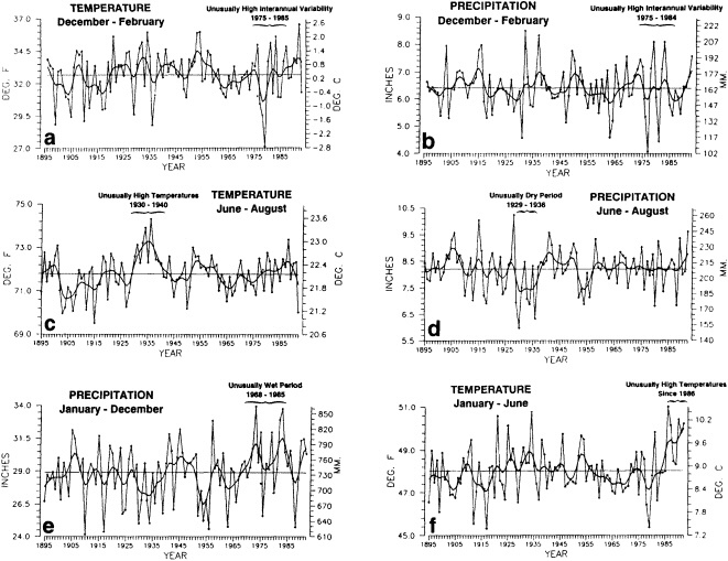
FIGURE 1
Time series of area-averaged seasonal and annual mean temperature and total precipitation for the contiguous United States. The smoothed curve is a nine-point binomial filter. The horizontal line reflects the mean over the period of record.
fying a mean climate state.) Nonetheless, there is evidence that climate fluctuations on longer time scales occur throughout the world (Jones and Briffa, 1995; Diaz and Bradley, 1995). As Karoly (1995) shows, there is a dearth of the data that would permit the identification of decadal-scale circulation variability in the Southern Hemisphere, but analysis of the longer-term surface data available suggests that significant climate fluctuations persist at least through decadal time scales.
The forcing agents of many climate fluctuations may have their origin in either anthropogenic or natural factors, or both. These fluctuations are important in terms both of their socioeconomic and biophysical effects and of our need to distinguish between natural climate variations and anthropogenic climate changes. In analyzing the climate record, the dangers of "data dredging" must be kept in mind. As access to climate data increases, the chance of finding trends and variations that appear to be significant also increases. For this reason decade-to-century-scale climate fluctuations have been referred to as the "gray area of climate change" (Karl, 1988). For instance, Keeling and Whorf (1995) find evidence for decadal fluctuations in the global temperature record that can be reproduced by assuming the existence of two oscillations with small differences in frequency that beat on time scales of about 100 years. The search for an explanation of this statistical result is a good example of the challenge presented by the existence of these decadal fluctuations.
IDENTIFYING CLIMATE FLUCTUATIONS
The instrumental record of atmospheric and related land and marine observations is fragmentary until at least the middle of the nineteenth century. Moreover, virtually all of
the observations used to study climate fluctuations are derived from observing programs that were developed not for this purpose, but rather to support day-to-day weather forecasting. Since the day-to-day variability of the atmospheric system in much of the world is far larger than the decadal climate variability, identification of multi-decadal climate fluctuations is often hampered by the poor quality and lack of homogeneity of the observations. For example, Groisman and Easterling (1995), in their study of the variability and trends of precipitation over North America, painstakingly document the many discontinuities and false jumps in the climate record that arise from changes in observing practices. These changes, if ignored, can and do overwhelm important long-term precipitation fluctuations.
Other atmospheric quantities besides precipitation are also affected by problems in measurement. In this section, Robinson (1995) points out the large disparity in snow-cover extent between a NASA data set using microwave measurements and a NOAA data set using visible imagery. Karl et al. (1995) devote considerable discussion to jumps and trends introduced into the surface temperature record by such factors as urban heat islands, changes in irrigation practices, differences in instrumentation, and station relocations. Cayan et al. (1995) use surface marine observations to calculate the latent and sensible heat fluxes that are used as forcing agents of the sea surface temperature field in the North Pacific. Their analysis includes the basin-wide climate jump that began about 1976-1977. To account for known systematic biases related to trends in the wind field and the sea surface and marine air-temperature and moisture lapse rates (Ward, 1992; Cardone et al., 1990; Wright, 1988; Ramage, 1987), the global trend of each of these quantities is removed. As mentioned in Zebiak's commentary on Cayan's paper, it is unfortunate that such adjustments to the data are necessary.
Often the corrections and adjustments that must be applied to a climate record are of such magnitude that it is difficult to be confident that the resulting time series adequately reflects the climate fluctuations. For example, Figure 2 illustrates the significant adjustments required to calculate global temperature fluctuations since the nineteenth century. Through the use of other data bases (e.g., changes in snow cover, alpine glaciers, or sea level) and the isolation of various components of the surface temperature record (e.g., marine air temperature, sea surface temperature, and land temperature), it is possible to gain more confidence in the adjustments applied. Each of the data sets has distinctly different problems related to long-term homogeneity and data quality that require independent adjustment procedures. When these independent data sets provide a physically consistent picture of decade-to-century climate fluctuations, their agreement can be very compelling. In fact, the analysis of quasi-periodic oscillations of surface winds, pressure, and ocean and marine air temperatures
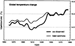
FIGURE 2
Smoothed global surface temperature variations, as derived from the original observations without adjustments for inhomogeneities in the climate record, compared to the same observations after adjustments for inhomogeneities as described by the Intergovernmental Panel on Climate Change (IPCC, 1990, 1992).
by Deser and Blackmon (1995) relies entirely on physical consistency among independent variables.
In order to improve our ability to discern climate fluctuations on decade-to-century time scales within the existing climate record, some federal agencies such as NSF, DOE, and NOAA are supporting data archeology efforts. Data archeology is the process of seeking out, restoring, correcting, and interpreting data sets. Such efforts are critical to identifying and understanding longer-scale climate fluctuations, since they often turn up information that reveals a pattern not otherwise obvious.
The Comprehensive Ocean-Atmosphere Data Set (COADS), which is just one of several major data-archeology efforts, provides a good example of the type of benefits that can be expected from such efforts. Now, several years after the project's inception (Woodruff et al., 1987), scientists are identifying decadal-scale variations and changes in many climate elements previously thought to be too uncertain to document with any confidence (London et al., 1991; Flohn et al., 1990; Parungo et al., 1994).
Interestingly, up to the present, satellite data have not figured prominently in the analysis of multi-decadal climate variability. Their short observing history and a lack of temporal homogeneity have hampered efforts to use them. Certainly, there are notable exceptions, such as NOAA's snow and sea-ice products and the Spencer and Christy (1990) microwave sounding-unit data. However, major temporal inhomogeneities in data sets, like those identified in the International Satellite Cloud Cover Project (ISCCP; see Klein and Hartmann, 1993), threaten the usefulness of much of the multi-decadal satellite data. The two major challenges over the next few decades for the United States will to be to ensure that global-change satellite-research projects such as EOS provide homogeneous data over their planned life-
times, and to lay the foundation for converting them into a long-term operational observing systems.
Future observations will require more attention to data quality, homogeneity, and continuity if we are to understand the nature of decade-to-century-scale climate variability. Currently under consideration is a Global Climate Observing System (GCOS)1 that includes observations of terrestrial, atmospheric, and oceanic aspects of climate. Since GCOS would be built around existing observing networks and environmental problems, it is essential that scientists effectively convey long-term climate-monitoring needs to the agencies sponsoring space-based and conventional observing systems. Among the climate-monitoring issues that should be addressed in the near future are stability of network sites, intercomparability of instruments, and increased sampling in data-sparse regions. Two concerns for both present and future observations are the better collection and documentation of metadata on observing instruments and practices as well as processing algorithms, and improved data-archiving practices and data-management systems. All these will increase the value of climate monitoring for decade-to-century-scale research; most essential, of course, is assurance of a long-term commitment to observational objectives.
THE FORCING AGENTS OF CLIMATE FLUCTUATIONS
The climate record provides the key to developing, refining, and verifying our hypotheses regarding the forcing agents responsible for climate fluctuations, be they anthropogenic or natural, internal or external to the climate system, global or regional, or persisting one or many decades. Diaz and Bradley (1995) suggest that the many decade-to-century climate fluctuations evident in both observations and proxy records may indeed have natural origins, since similar fluctuations seem to occur in the climate record both before and after humans became capable of modifying climate.
Often physically based models are the best means of testing our hypotheses about the cause of the fluctuations, as described in the modeling sections of this volume, but in addition they can be effectively used to help discern the physical consistency of apparent climate fluctuations and change. Cayan et al. (1995) demonstrate this approach; they use an ocean general-circulation model to help explain the climate jump over the North Pacific, as documented by Trenberth (1990; Trenberth and Hurrell, 1995, in this volume). Cayan et al. show how the atmosphere and ocean can act together to maintain decadal-scale climate fluctuations on a large spatial scale.
Potentially important factors in explaining climate fluctuations on decade-to-century time scales are land-surface and atmospheric feedback effects. Walsh (1995) provides ample evidence that snow cover has important feedback effects on the climate system on short (daily and interannual) and long (thousands of years) time scales, but on the time scales of interest to us the impact of snow is still not well understood. However, Nicholson (1995) and Shukla (1995) present evidence that the feedback between land-surface characteristics and the atmosphere has led to the prolonged drought in the Sahel. Karl et al. (1995) document an asymmetric increase of the mean maximum and minimum temperatures over many portions of the global land mass. Although they cite a number of potential causes of this multi-decadal trend, such as increases of anthropogenic atmospheric sulfate aerosols (Charlson et al., 1992) and greenhouse gases, empirical evidence suggests that, at least in some regions, observed increases in cloud cover play an important role in modulating the surface temperature. The forcing responsible for the increase in cloud cover remains unknown.
There are many important aspects of climate forcings and associated responses that cannot be covered here. Of particular relevance are the known changes in solar irradiance associated with the sunspot cycle. Recently Friis-Christensen and Lassen (1991) have used the length of the sunspot cycle to explain the decadal fluctuations and trends of land temperatures. Although a linear response of the surface temperature to the sunspot cycle length implies some unlikely responses of the temperature record in the early part of the time series (Kelly and Wigley, 1992), it is clear that changes in solar irradiance must continue to be monitored as a potential source of global climate fluctuations or change.
Recently, Elliott et al. (1991) have found evidence for an increase of tropospheric water vapor since 1973, leading to an enhanced greenhouse effect. However, the many types of observing and data-processing inhomogeneities in the upper-air moisture record make it immensely difficult to separate spurious trends and discontinuities from the true climate signal, even when the signal may be as large as a 10 percent increase in specific humidity.
A critical atmospheric quantity affecting surface temperature is the variability of cloud cover—its type, height, and spatial distribution. Using the ISCCP data base, Hartmann et al. (1992) showed the net forcing of various cloud types as a function of season and latitude. A recent study by Rossow (1995), however, reveals that this data set has serious biases that make it inappropriate for decadal-scale climate assessments. Meanwhile, conventional in situ data, analyzed on a national basis by a number of researchers, show a widespread general increase in total cloud cover
over the past several decades (Dutton et al., 1991; Henderson-Sellers, 1990; Karl and Steurer, 1990; London et al., 1991; McGuffie and Henderson-Sellers, 1989; Parungo et al., 1994). Clearly, a much more focused effort is required to better understand decadal and multi-decadal fluctuations of cloud cover, since they often have very important feedback effects on other climate quantities. For instance, cloud feedbacks work differently during the day from the way they do at night. They therefore differ at high and low latitudes, making generalizations speculative.
Also, there is no discussion in this volume of the world's glaciers, in spite of their known tendency to fluctuate markedly on decade-to-century time scales. Long-term trends of climate change are integrated by mountain glaciers, and during the past century mountain glaciers all over the world have been declining (IPCC, 1990). The World Glacier Monitoring Service (1993) summarized these changes over the past several decades, and the USGS Satellite Image Atlas of the World discusses observed variations of hundreds of glaciers over the past several centuries.
CONCLUSION AND RECOMMENDATIONS
Identification and explanation of the forcings and feedbacks responsible for decade-to-century-scale climate fluctuations are essential to distinguishing between natural and anthropogenic impacts on the climate system, as well as to developing any predictive skill with respect to these phenomena. Further progress in understanding this gray area of climate change will depend upon our ability to address three topics. First, we must be able to document climate fluctuations without spurious discontinuities and trends. Second, we must ensure that we are adequately monitoring potential forcings and feedbacks internal and external to the climate system, so that we will have the data necessary for testing hypotheses about their operation. Last, data analysts must work closely with modelers (and vice versa) to test the hypotheses we formulate on a variety of climate models, ranging from simple one-dimensional climate models to complex coupled ocean-atmosphere general-circulation models. The re-analysis modeling projects of the United States (Kalnay and Jenne, 1991) and the European community are likely to enhance our confidence in both how and why climate has varied on decade-to-century time scales. (It must be emphasized, however, that the value of any re-analysis effort can be jeopardized by the use of data that are biased or, most troublesome, inhomogeneous in time.) Only by advancing in all three of these areas will we be able to overcome our ignorance about multi-decadal climate fluctuations and make predictions with any degree of assurance.
Documenting Natural Climatic Variations: How Different is the Climate of the Twentieth Century from That of Previous Centuries?
HENRY F. DIAZ1 AND RAYMOND S. BRADLEY2
ABSTRACT
Changes in decadal-mean surface temperature and its variance for different land areas of the Northern Hemisphere are examined. In the last 100 years, changes in surface air temperature have been greatest and most positive in the period since about 1970. Interannual variability, particularly at the largest spatial scales has also increased, although it differs according to regions. The most unusual decade of the last 100 years in the contiguous United States may have been the 1930s, although that of the 1980s is probably a close second, and in some regions perhaps the most anomalous. Both the 1930s and the 1980s experienced significant warming together with enhanced climatic variability.
To incorporate a longer-term perspective than is obtainable from the modern instrumental record, we used summer temperature reconstructions based on tree-ring records, and on d18O ratios extracted from different ice-core records. Although none of these records is a simple or even direct temperature proxy, we present them as general indicators of prevailing environmental temperatures. The data were averaged by decades in order to focus on decadal-scale variability. With the exception of the data from tropical ice cores, the proxies indicate that the recent decades were not very unusual, either in regard to the mean or in terms of increased variability. While seasonal and annual temperature changes in the last two decades have been rather large in most areas of the Northern Hemisphere, the available paleoclimate evidence suggests that in many areas there have been decadal periods during the past several centuries in which reconstructed temperatures were comparable to those of the 1970s and 1980s, with climatic variability as large as any recorded in recent decades. Natural variability on decadal time scales is comparatively large—typically about half as large as the interannual variance.
INTRODUCTION
Considerable effort has been expended over the last 25 years to improve our knowledge and understanding of climate processes and mechanisms associated with changes in climate (Saltzman, 1983; Trenberth, 1992). A major impetus for much of the recent climate research has been the global and regional climate projections made with physical climate models (the so-called general-circulation models, or GCMs) for a doubling of carbon dioxide concentration in the atmosphere.
Most assessments of the climatic impact of increases in the ''greenhouse" gases (CO2, methane, nitrous oxide, chlorofluorocarbons) have concluded, more or less consistently, that global temperatures should rise (under a doubling of the most abundant of these greenhouse gases, CO2) from 1.5°C to 4.5°C (NRC, 1982; Bolin et al., 1986; IPCC, 1990; Schlesinger, 1984, 1991). Such changes, should they occur, will be superimposed on the natural variability of the climate, which is quite large at all time scales (Karl et al., 1989). Depending on a number of assumptions, the amount of global warming that should have been realized by now appears to be more consistent with the lower end of the above estimates (Bloomfield, 1992).
Karl et al. (1991b) performed a variety of tests using output from three different GCMs to ascertain, given their different climate sensitivities, when a statistically significant greenhouse signal might be detected in the central United States. They concluded that it was likely that a greenhouse signal had been masked, to date, by natural climate variability, and that it would likely take another two to four decades before the greenhouse signal in temperature and precipitation might be unambiguously detected in this region.
We should note the possibility that other human-induced factors may be acting to counteract the radiative effects of increased greenhouse-gas concentrations in the atmosphere. Recent work has indicated that sulfate aerosols, which act to increase the planetary albedo (Charlson et al., 1992; Hansen and Lacis, 1990; Wigley, 1989, 1991) may have counteracted to some degree the enhanced infrared warming (see Michaels and Stooksbury, 1992). These and other factors, whether anthropogenic in origin or not (e.g., changes in vulcanism), will undoubtedly "muddy" the climate picture and may make it more difficult to identify unequivocally a contemporary greenhouse signal.
In this paper, we consider two aspects of climate-change detection that we feel bear strongly on the issue of natural versus anthropogenic climate variability. One aspect of the problem is, in effect, at what point one rejects the null hypothesis (no climate change) and accepts the premise that the climate of the last few decades belongs to a different sample population. The difficulty there arises because we are evaluating a relatively short observational record with the knowledge that the climate has fluctuated in the past few centuries by an amount that may be of the same magnitude as the fluctuations observed in the recent record (see Bradley and Jones, 1992).
A second aspect of the problem of climate change versus natural variability, which we consider here, is temporal changes in that variability, i.e., in the variance. Changes in climatic variability are important, since they are likely to have a greater effect on a society's ability to mitigate and adapt to climatic changes than a slow alteration in the mean climate patterns. We have examined a variety of observational records of various lengths (typically 100 to 150 years), which are representative of different spatial scales (from hemispheric to regional basins). We will focus on decadal time scales, since one could argue that climatic changes will be better gauged at time scales that to some extent average out the high-frequency climatic "noise" associated with seasonal variability and other air-sea processes operating on annual time scales (e.g., the El Niño/ Southern Oscillation system). We compare these instrumental series with a suite of high-resolution climate proxy records—namely, tree rings and oxygen isotopes extracted from ice cores—spanning the last 300 to 800 years. Our aim is to give the reader some feeling for the range of this intermediate-frequency (decade-to-century-scale) climatic variability, as well as some appreciation of the uncertainties inherent in the existing records (instrumental, historical, and paleoenvironmental).
We note that the "fingerprint" climate-change-detection technique (Barnett, 1986; Barnett and Schlesinger, 1987; Barnett et al., 1991) provides a very useful methodology for testing a hypothesis (the GCM climate-change projections) against observations. We will attempt here to highlight some aspects of climatic variability at decadal and longer time scales and will re-emphasize the conclusion of Barnett et al. (1991), who noted that the existence of a high degree of "unexplained" interdecadal climatic variability (see also Ghil and Vautard, 1991, and Karl et al., 1991b) will greatly complicate the detection of a greenhouse climate-change signal.
THE MODERN (INSTRUMENTAL) RECORD
Characteristics of Decadal-Scale Changes of Area-Mean Temperature Indices
The available data suggest that during the past century decadal-scale changes in global-scale mean annual temperature are on the order of 0.1°C to 0.3°C (see Folland et al., 1990). Figure 1 illustrates the annual and seasonal temperature changes for the Northern Hemisphere land areas. The plotted data, from Jones et al. (1986a) with subsequent updates, are consecutive 10-year area-weighted averages from 1891-1900 through 1981-1990 of gridded temperature anomalies referenced to the 1951-1970 period. On this "dec-
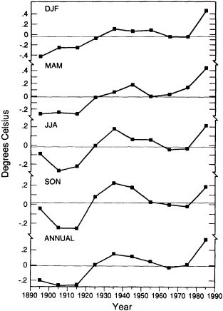
FIGURE 1
Decadal-mean seasonal and annual temperature anomalies (in °C) for land areas of the Northern Hemisphere. Data is from Jones et al. (1986a), with subsequent updates.
adal" time scale, the warming of the 1980s relative to the 1970s (0.32°C for the hemisphere) is comparable to the warming that occurred in the 1920s relative to temperatures in the 1910s (0.26°C). Some seasonal differences can be noted, with northern summer and fall showing the least warming trend and winter and spring showing the greatest warming trend over the last 100 years.
The twentieth century contains many examples of decadal-scale climatic variations of sufficient magnitude to have significantly affected societies. The two-decade-long drought in the African Sahel is perhaps the best-known example. The words "climate change" have become overused, and climatic variations from seasonal to multi-year are often lumped together. Until the mid-1970s, "climate change" was used to refer to climatic changes on time scales of 104 to 106 years (essentially, Milankovitch time-scales). Variations of less than 10 years were generally considered to be part of the natural climate noise associated with interannual variations of the various components of the climate system and their nonlinear interactions, whereas variations on time scales of 10 to 103 years are now thought to be strongly driven by ocean-atmosphere heat exchanges resulting from changes in the ocean's thermohaline circulation.
Because of the changes in the earth's radiative balance imposed by human activities during the past century, climatologists have been trying to detect climatic-change signals that hitherto have typically been associated with time scales of millennia. The climate record available for such studies, even with the aid of high-resolution paleoenvironmental records, is sufficient to define only continental to hemispheric changes on decadal time scales, and perhaps regional (less than about 105 km2) changes on century time scales.
In the United States, perhaps the singular climatic event of this century was the severe, widespread, and persistent drought of the 1930s. This event has been widely chronicled in both scientific (e.g., Skaggs, 1975) and popular literature. Other climatic events that persisted for more than one year and affected relatively large areas of the United States were the drought of the 1950s in south central areas of the United States (Chang and Wallace, 1987), and the drought of the 1960s in the Northeast (Namias, 1966). Periodic drought of variable duration has affected all areas of the contiguous United States to varying degrees (Diaz, 1983). Indeed, multiyear climate anomalies are a characteristic feature of the climate of the United States and of other parts of the world (Karl, 1988; Folland et al., 1990).
In Figure 2, decadal-mean seasonal (December-February for winter, March-May for spring, etc.) and annual temperature anomalies for various areas of the Northern Hemisphere are examined. Although Eurasia and North America (Figure 2a) have broadly similar seasonal trends over this period, differences can be noted in all seasons as well as in the annual averages. Figure 2b illustrates decadal temperature changes for the contiguous United States for the last century. The data used are from the adjusted divisional values (solid curve) described in Karl et al. (1984b). For comparison, the equivalent Jones et al. (1986a) gridded values are given as the dashed curve in Figure 2b. The decadal averages for the lower 48 states exhibit much smaller long-term trends than those noted for the continental-scale regions. Figures 2c and 2d illustrate the decadal temperature changes recorded in subregions of the United States, namely, the eastern and western halves of the United States (divided roughly along the 100th meridian), the state of Colorado, and a single state climatic division in Colorado where the city of Boulder is located. Again we note regional differences that can depart substantially from the temporal behavior of the larger spatial averages.
We have tabulated the mean temperature change from one calendar decade to the next over the 100-year period 1891 to 1990 for each of the above regions. No particular pattern emerges, except that at the largest space scales, the greatest decade-to-decade warming occurs mostly from the 1970s to the 1980s, whereas the time of the largest such
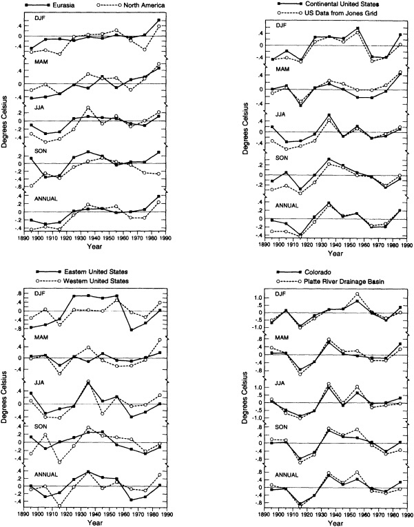
FIGURE 2
Decadal-mean seasonal and annual temperature anomalies (in °C). (a) For the Eurasian (solid line) and North American (dashed line) land masses. (b) For the contiguous United States, using data from the National Climatic Data Center described in Karl et al. (1984b) (solid line) and from the gridded temperature anomaly fields of Jones et al. (1986a) (dashed line). (c) For the eastern (solid line) and western (dashed line) United States. (d) For the state of Colorado (solid line) and the Platte River climatic division of Colorado (dashed line).
changes varies for the smaller regional averages, with most areas of the contiguous United States experiencing their greatest decadal changes during the first half of this century.
Recent studies have documented some rather pronounced and relatively rapid shifts in the climate system that occurred on decadal time scales. In particular, the atmospheric circulation in the extratropical North Pacific underwent a major shift in the mid-1970s that lasted over 10 years (Trenberth, 1990; Ebbesmeyer et al., 1991). This change was accompanied by a tendency for climate patterns in the tropical Pacific to exhibit conditions reminiscent of El Niño/Southern Oscillation (ENSO) warm-event conditions—weaker trades, warmer equatorial sea surface temperature (SST), anomalous rainfall patterns, etc.—relatively more frequently than during previous decades. Gordon et al. (1992) have also reviewed some of the relatively abrupt changes in water properties and surface climate in the Atlantic Ocean that have occurred in the past several decades, including sudden changes in SST anomalies in the South Atlantic compared to those of the North Atlantic, and the so-called "great salinity anomaly" in the North Atlantic from about the late 1960s to the early 1980s (Dickson et al., 1988). Certainly the sudden decrease of rainfall in the Sahel of Africa, a feature that has lasted for two decades, is a good example of how the climate can undergo significant, sudden, and prolonged change over relatively large spatial scales.
Clearly, increased knowledge of the behavior of climatic variability, from the interannual through decadal and century time scales, is needed to improve our assessments of any future changes in climate from regional to global scales. Indeed, as was noted by Ghil and Vautard (1991), the ability to distinguish a warming trend from natural variability is critical for separating out the greenhouse-gas-induced signal.
As we noted at the outset, an important element of climate that is too often overlooked is the variance or the characteristic variability of climatic means. In determining climate impacts, the importance to society of short- to medium-term climatic instability (i.e., climate fluctuations occurring on interannual to interdecadal time scales) is perhaps equal to or greater than that of slow changes in the background mean. Below we have analyzed some aspects of low-frequency changes in the temperature variance of different regional means.
Changes in Temperature Variability
We have examined contemporaneous variation of two measures of temperature variability, the standard deviation in running 15-year segments, and decadal means of the root-mean-square differences between successive yearly values of seasonal and annual regional temperature anomalies. The latter index is defined as
Since the xi are deviations from a reference mean and have approximately zero mean,
where s2 is the series variance, and r1 is the autocorrelation of the time series with a lag of I year. We will use this measure, rather than the standard deviation, as the key index of interannual variability. Note that this index, Ind V, amplifies changes in the high-frequency part of the variance spectrum.
Figures 3 and 4 illustrate the changes in the interannual variability of the regional groupings discussed earlier. The curves differ from one season to another and from one region to another. For the largest continental-sized regions, there appears to be an increase in interannual variability in the last couple of decades. At smaller spatial scales, there does not seem to be a consistent trend; instead, the interan-
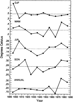
FIGURE 3
Index of interannual variability (in °C) for the Northern Hemisphere land areas. Values correspond to decadal means of the root-mean-square difference between successive seasonal and annual temperature anomalies over the last 100 years.
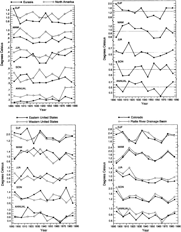
FIGURE 4
Indices of interannual variability, as in Figure 3. (a) For the Eurasian (solid line) and North American (dashed line) landmasses. (b) For the contiguous United States, using data from the National Climatic Data Center. (c) For the eastern (solid line) and western (dashed line) United States. (d) For the state of Colorado (solid line) and the Platte River climatic division of Colorado (dashed line).
nual variability wanes and waxes over the last 100 years. The corresponding curves for the standard deviation (not shown) reveal similar patterns, with increases in variance at the largest spatial scales with time but no consistent trends in the standard deviation of the smaller regions. As one would expect, there is a well-defined log-linear relationship between the magnitude of the interannual variability and the size of the area comprised by the various indices (see Figure 5). The inherently higher variability at smaller regional scales should be kept in mind when interpreting the paleoclimate record, which is based on limited regional samples.
The question of whether a warming climate will exhibit increased short-term variability is still open. Previous studies have been generally inconclusive on this subject (van Loon and Williams, 1978; Diaz and Quayle, 1980). Certainly, there is no consistent relationship between interdecadal changes in average temperatures and interdecadal changes in variability. Climatic variability may increase, decrease, or stay the same, in response to an arbitrary change in decadal mean temperatures. On the basis of the above results, we can say that, considering surface temperature variations during the last century, there has been a recent increase in variability at large spatial scales (continental to hemispheric-scale averages). This increase in variability is also concurrent with relatively large temperature increases over those areas. However, this is not the case for earlier warming episodes.
THE PRE-INSTRUMENTAL PERIOD
Prior to the late 1800s, reliable quantitative data on climate variations are sparse, and conclusions about the magnitude of these changes on large spatial scales necessarily contain significant degrees of uncertainty. There is ample evidence that multi-decadal temperature changes occurring over regions the size of Europe and China have been at least of order 1°C (Bradley and Jones, 1992). This suggests that it is quite plausible, if not likely, that temperatures as warm as those prevailing since the end of the Second World War may have been experienced at regional spatial scales of about 105 to 106 km2 for periods of one to several decades during some portions of the past thousand years under what amounts to natural (i.e., with negligible human influences) conditions.
Below we present some examples of long-term variability in a set of climate-sensitive paleotemperature records. The climate indices used here are discussed in several chapters of Bradley and Jones (1992). A listing of them, together with the source references and periods of record, appears in Table 1; each of them has been assigned a number for use in later tables comparing their data. Because of its very long record, the instrumental temperature series for central England (Manley, 1974) is considered in this section for comparison with other paleoclimate indices.
Tree-Ring Indicators
There is an extensive body of work relating climate variations to growth changes in particularly climate-sensitive trees (e.g., Fritts, 1976; Fritts et al., 1979; Hughes et al., 1982; Cook and Kairiukstis, 1990). We have selected a suite of climate-sensitive tree-ring records to study possible changes in climatic variability. Two main considerations were applied in the selection of these indices. First, we chose
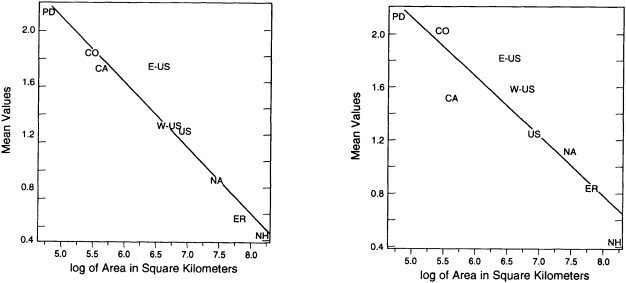
FIGURE 5
Interannual variability (in °C) as a function of the regional area. Values shown are for northern summer (left panel), and winter (right panel). Area is plotted as log10 values.
TABLE 1 Temperature Indices Used in This Study
|
Type of Record |
Time Coverage |
Reference |
Index No.* |
|
Ice-core d18O |
|||
|
Agassiz Ice Cap (Ellsmere Is.) |
A.D. 1349-1977 |
Fisher and Koerner (1983) |
1 |
|
Devon Island Ice Cap |
A.D. 1512-1973 |
Koerner (1977) |
2 |
|
Camp Century (Greenland) |
A.D. 1176-1967 |
Johnsen et al. (1972) |
3 |
|
Milcent (Greenland) |
A.D. 1176-1967 |
Hammer et al. (1978) |
4 |
|
Quelccaya Ice Cap (Peru) |
A.D. 1481-1981 |
Thompson et al. (1986) |
14 |
|
Dunde Ice Cap (China) |
A.D. 1606-1987 |
Thompson et al. (1990) |
15 |
|
Temperature reconstructions from tree rings |
|||
|
Western U.S. (annual) summer |
A.D. 1602-1961 |
Fritts (1991) |
5 |
|
Eastern U.S. (annual) summer |
A.D. 1602-1961 |
Fritts (1991) |
6 |
|
Western U.S. & SW Canada (annual) summer |
A.D. 1602-1961 |
Fritts (1991) |
7 |
|
Northern Treeline (North America) (annual) |
A.D. 1601-1974 |
D'Arrigo & Jacoby (1992) |
9 |
|
U.S. & SW Canada (April-September) |
A.D. 1600-1982 |
Briffa et al. (1992b) |
8 |
|
Northern Scandinavia (April-August) |
A.D. 500-1980 |
Briffa et al. (1992a) |
12 |
|
Northern Urals (June-July) |
A.D. 961-1969 |
Graybill and Shiyatov (1992) |
13 |
|
Tasmania, Australia (November-April) |
A.D. 900-1989 |
Cook et al. (1992) |
16 |
|
Patagonia, Argentina (December-April) |
A.D. 1500-1974 |
Boninsegna (1992) & Villalba et al. (1989) |
17 |
|
Rio Alerce, Argentina (December-February) |
A.D. 870-1983 |
Villalba (1990) |
18 |
|
Instrumental |
|||
|
Central England Temperature (annual) |
A.D. 1660-1987 |
Manley (1974) |
|
|
Dec-Jan-Feb series |
|
|
10 |
|
June-July-Aug series |
|
|
11 |
|
* These numbers are used in text and later tables to identify the various indices. |
|||
climate-sensitive tree-ring records that have been thoroughly documented in the refereed scientific literature. Second, we chose the longest of those records in order to maximize the temporal coverage, and tried, as far as possible, to select samples from representative geographical areas.
A number of problems are inherent in any climate reconstruction. These problems are discussed in detail in the original published papers; however, we will briefly highlight here the more critical ones as they may affect the results presented below. Because we have analyzed changes in variability, temporal changes in the composition of the tree-ring network used for the reconstructions will, in general, affect the high-frequency variance, and to some degree the low-frequency variance as well. In interpreting the temperature reconstructions shown here, we have taken into account these potential sources of biases as much as possible.
Regardless of whether one uses the width of the annual growth rings or the maximum latewood density to reconstruct a particular climate variable (generally, growing-season temperature and/or precipitation), a process of standardization is required to account for different rates of tree growth as a function of age. This standardization is achieved by fitting a growth curve to the series of annual values, usually a cubic smoothing spline (see Cook and Kariukstis, 1990), and taking residuals about the smoothed curve. The degree of smoothing and the functional form of the growth curve partly determine the spectral properties of the residual series. In order to develop a climate reconstruction from these records, it is necessary to formulate a transfer function to convert the tree-growth index into, say, a temperature index. The procedure usually involves a calibration phase, in which a set of regression coefficients is derived that convert the tree-growth parameter into a climatic estimate, and a verification phase (see, e.g., Cook
and Kariukstis). Verification is usually done against an independent set of predictors. The reader is urged to review the reference sources listed in Table 1 for specific details regarding each paleotemperature reconstruction.
Another feature of long-term reconstructions from tree rings that should be borne in mind is that the composition of tree-ring samples that make up each yearly value is variable. In general, an index value for a given site is composed of a number of tree samples from several individual trees. These may vary in age, and in some cases may come from both dead as well as living trees. The number of samples making a particular ensemble average will vary with time, although this is more generally the case near the beginning and end of a particular chronology. These extraneous factors can introduce "noise" and spurious fluctuations into the reconstructions. Nevertheless, the tree-ring indices considered here, while suffering to varying degree from the above-named shortcomings, comprise a high-quality set of proxy temperature records that are of value to compare.
Figures 6 through 8 show decadal-mean values of various tree-ring reconstructions, generally representing summer (or growing-season) mean temperature. For the most part, these tree-ring reconstructions do not sample the 1980s; nevertheless, it is clear from the degree of interdecadal variability that it would be hard to point to any particular recent period as being unique or exceptional. The November-to-April
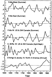
FIGURE 6
Decadal mean values of reconstructed summer- temperature anomalies for various North American regions. The top three graphs are in standardized units, the bottom two are in °C. See Table 1 for source information.
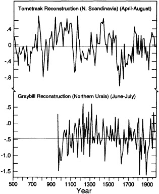
FIGURE 7
Decadal mean values of reconstructed summer temperature anomalies for Scandinavia and the northern Urals. Units in °C.
temperature reconstruction for Tasmania (Cook et al., 1992) does indicate that the last two decades of that record (1970s and 1980s) exhibit significantly greater tree growth (Figure 8) and hence higher reconstructed mean growing-season temperatures than previously, but it would seem premature to conclude that a "climatic change" has taken place in this region of southern Australia. We also note that, unlike the North American and Scandinavian reconstructions, this one is based on tree samples from only one location.
Some unique features are evident for a few of the temperature indices. For example, the curve of D'Arrigo and Jacoby (1992) is a reconstruction of annual mean temperature based on several sites along the northern North America treeline, stretching from Alaska to the Northwest Territories, plus a site located in northern Quebec Province. This reconstruction exhibits a pronounced warming from a very cold period during the mid-1800s to a maximum around 1940. By comparison, the two other high-northern-latitude sites discussed here—the indices from northern Scandinavia and from the northern Urals (Figure 7)—do not exhibit quite the same type of variations. The reader should note, however, that a much longer time period is sampled by these other two reconstructions, and that a seasonal (April to August for the Tornetrask index, and June to July for the
TABLE 2 Century Means of Interannual and Interdecadal Variability for 18 Temperature Indices (index sources identified in Table 1)
|
|
Index |
|||||||||||||||||
|
Century |
1 |
2 |
3 |
4 |
5 |
6 |
7 |
8 |
9 |
10 |
11 |
12 |
13 |
14 |
15 |
16 |
17 |
18 |
|
500s (ann.) |
x |
x |
x |
x |
x |
x |
x |
x |
x |
x |
x |
.84 |
x |
x |
x |
x |
x |
x |
|
(decad.) |
x |
x |
x |
x |
x |
x |
x |
x |
x |
x |
x |
.20 |
x |
x |
x |
x |
x |
x |
|
600s (ann.) |
x |
x |
x |
x |
x |
x |
x |
x |
x |
x |
x |
.79 |
x |
x |
x |
x |
x |
x |
|
(decad.) |
x |
x |
x |
x |
x |
x |
x |
x |
x |
x |
x |
.27 |
x |
x |
x |
x |
x |
x |
|
700s (ann.) |
x |
x |
x |
x |
x |
x |
x |
x |
x |
x |
x |
.64 |
x |
x |
x |
x |
x |
x |
|
(decad.) |
x |
x |
x |
x |
x |
x |
x |
x |
x |
x |
x |
.40 |
x |
x |
x |
x |
x |
x |
|
800s (ann.) |
x |
x |
x |
x |
x |
x |
x |
x |
x |
x |
x |
.63 |
x |
x |
x |
x |
x |
x |
|
(decad.) |
x |
x |
x |
x |
x |
x |
x |
x |
x |
x |
x |
.35 |
x |
x |
x |
x |
x |
x |
|
900s (ann.) |
x |
x |
x |
x |
x |
x |
x |
x |
x |
x |
x |
.70 |
.27 |
x |
x |
,x |
x |
.87 |
|
(decad.) |
x |
x |
x |
x |
x |
x |
x |
x |
x |
x |
x |
.31 |
.18 |
x |
x |
x |
x |
.41 |
|
1000s (ann.) |
x |
x |
x |
x |
x |
x |
x |
x |
x |
x |
x |
.66 |
1.95 |
x |
x |
.53 |
x |
.71 |
|
(decad.) |
x |
x |
x |
x |
x |
x |
x |
x |
x |
x |
x |
.25 |
.53 |
x |
x |
.25 |
x |
.28 |
|
1100s (ann.) |
x |
x |
x |
x |
x |
x |
x |
x |
x |
x |
x |
.69 |
1.70 |
x |
x |
.62 |
x |
.46 |
|
(decad.) |
x |
x |
x |
x |
x |
x |
x |
x |
x |
x |
x |
.43 |
.56 |
x |
x |
.20 |
x |
.14 |
|
1200s (ann.) |
x |
x |
1.36 |
1.25 |
x |
x |
x |
x |
x |
x |
x |
.69 |
1.85 |
x |
x |
.43 |
x |
.59 |
|
(decad.) |
x |
x |
.53 |
.85 |
x |
x |
x |
x |
x |
x |
x |
.22 |
1.02 |
x |
x |
.16 |
x |
.29 |
|
1300s (ann.) |
.93 |
x |
1.10 |
1.36 |
x |
x |
x |
x |
x |
x |
x |
.68 |
2.47 |
x |
x |
.42 |
x |
.68 |
|
(decad.) |
.39 |
x |
.65 |
.68 |
x |
x |
x |
x |
x |
x |
x |
.30 |
.66 |
x |
x |
.30 |
x |
.19 |
|
1400s (ann.) |
.70 |
x |
1.38 |
1.27 |
x |
x |
x |
x |
x |
x |
x |
.68 |
2.02 |
x |
x |
42 |
x |
.65 |
|
(decad.) |
.47 |
x |
.68 |
.33 |
x |
x |
x |
x |
x |
x |
x |
.23 |
.47 |
x |
x |
.18 |
x |
.32 |
|
1500s (ann.} |
.78 |
.59 |
1.13 |
1.18 |
x |
x |
x |
x |
x |
x |
x |
.60 |
1.75 |
1.86 |
x |
.42 |
.96 |
.62 |
|
(decad.) |
.85 |
.69 |
.65 |
.67 |
x |
x |
x |
x |
x |
x |
x |
.37 |
.56 |
.74 |
x |
.17 |
.23 |
.14 |
|
1600s (ann.) |
.89 |
.71 |
1.27 |
1.43 |
.45 |
.32 |
.31 |
.63 |
.22 |
x |
x |
.69 |
1.63 |
1.80 |
1.12 |
.50 |
.56 |
.66 |
|
(decad.) |
.50 |
.64 |
.59 |
.47 |
.30 |
.41 |
.21 |
.42 |
.25 |
x |
x |
.43 |
.53 |
.66 |
.49 |
.14 |
.14 |
.19 |
|
1700s (ann.) |
.84 |
.62 |
1.05 |
1.36 |
.42 |
.31 |
.25 |
.53 |
.23 |
1.81 |
.98 |
.74 |
1.85 |
2.01 |
1.11 |
.49 |
.53 |
.65 |
|
(decad.) |
.96 |
.27 |
.87 |
.54 |
.21 |
.26 |
.14 |
.20 |
.34 |
.77 |
.25 |
.43 |
.40 |
.70 |
.55 |
.22 |
.18 |
.28 |
|
1800s (ann.) |
.97 |
.78 |
1.25 |
1.21 |
.52 |
.35 |
.29 |
.54 |
.21 |
1.89 |
1.18 |
.84 |
1.64 |
1.67 |
1.10 |
.45 |
.53 |
.75 |
|
(decad.) |
1.07 |
.55 |
.62 |
.77 |
.26 |
.29 |
.21 |
.23 |
.26 |
.31 |
.50 |
.35 |
.95 |
.96 |
.29 |
.17 |
.18 |
.38 |
|
1900s (ann.) |
1.51 |
1.02 |
1.38 |
1.67 |
.51 |
.33 |
.29 |
.53 |
.27 |
1.67 |
1.14 |
.71 |
1.78 |
1.24 |
1.28 |
.45 |
.62 |
.76 |
|
(decad.) |
.52 |
.49 |
.72 |
.44 |
.30 |
.33 |
.23 |
.23 |
.27 |
.53 |
.35 |
.27 |
.68 |
1.10 |
.59 |
.21 |
.22 |
0.33 |
TABLE 3 Long-term Means of Interannual and Interdecadal Variability for 18 Temperature Indices (index sources identified in Table 1)
|
Index |
||||||||||||||||||
|
|
1 |
2 |
3 |
4 |
5 |
6 |
7 |
8 |
9 |
10 |
11 |
12 |
13 |
14 |
15 |
16 |
17 |
18 |
|
LTM (ann) |
.95 |
.75 |
1.24 |
1.33 |
.47 |
.33 |
.29 |
.56 |
.23 |
1.86 |
1.09 |
.71 |
1.91 |
1.74 |
1.15 |
.46 |
.66 |
.68 |
|
LTM (dec) |
.75 |
.55 |
.66 |
.62 |
.27 |
.33 |
.20 |
.29 |
.28 |
.59 |
.41 |
.33 |
.67 |
.82 |
.49 |
.20 |
.19 |
.27 |
|
Ratio (%) |
79 |
74 |
54 |
46 |
56 |
100 |
69 |
51 |
122 |
32 |
38 |
47 |
35 |
47 |
42 |
44 |
29 |
39 |
northern Urals set) interval rather than annual periods is considered.
The two summer temperature reconstructions for South America (Figure 8) are of widely different lengths. A comparison of the overlap period indicates that the Boninsegna series (see Table 1) exhibits a warming trend over the period of record. By contrast, the longer Villalba series exhibits some low-frequency variations but little if any trend over both the full data period and that of the Boninsegna period, beginning about the mid-fifteenth century.
Because of the longer record available, a variability index (described in the section on instrumental data above) was computed using the decadal averages, instead of the annual values. Our purpose here is to examine interdecadal temperature variability, with records spanning several centuries, noting that climate-sensitive tree-ring records are particularly useful for studying decadal-scale climatic fluctuations (Fritts, 1991). The changes in reconstructed climatic vari-
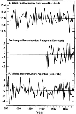
FIGURE 8
Decadal mean values of a reconstruction of summer temperatures for Tasmania, Australia (shown as actual temperatures) and two separate reconstructions for regions in Patagonia, Argentina (shown as anomalies). Units in °C.
ability have been summarized on a century-by-century basis in Table 2. For comparison, we also show in Table 3 the mean values of interannual and interdecadal variability for the full-length record. The variability index was calculated by applying equation (1) to both the annual and decadal-average reconstructed series. We fail to see any consistent trends in interdecadal variability associated with these tree-ring temperature reconstructions (see indices 5-9, 12-13, and 16-18 in Table 2). Interdecadal variability is typically about half the interannual values. This implies that substantial low-frequency variance is present in the paleotemperature record, so that recent high values of reconstructed decadal-mean summer temperature may yet represent an oscillation within the range of natural variability.
Oxygen Isotopes
The oxygen-isotope record has not been directly calibrated against temperature, as has been done for the tree-ring record. However, it is well established that the oxygen-isotope ratio (d18O) is dependent primarily on the temperature of formation of the precipitation, with increasingly negative d18O ratios associated with decreasing temperature. The problems lie in the interpretation of a local ice-core record, not only with respect to local temperature variations, but even in terms of the larger-scale temperature patterns. Several factors control the oxygen-isotope composition of the snow that falls on a given ice body, and temperature is only one of them. The sensitivity of these records to annual temperature variations has been discussed in a number of papers, including the source articles referred to in Table 1. Whether or not these oxygen-isotope records accurately represent a "local" temperature record, we consider them to be sensitive indicators of prevailing climatic conditions within a suitably broad source region. Since our stated purpose is to compare recent changes in a suite of climate-sensitive paleoindicators, we have included them in our comparisons.
Figures 9 and 10 illustrate the changes in decadal averages of the oxygen-isotope ratio of glacier ice cores for different locations in northern Canada and Greenland, and for two low-latitude, high-elevation glaciers (the Quelccaya ice cap in the Peruvian Andes and the Dunde ice cap in the Tibetan Plateau region of China (see Table 1 for sources)). The polar ice d18O record, which ends before 1970, shows relatively less warming (trend toward smaller negative values of d18O) than do the tropical ice cores. Furthermore, the warmest decades in the tropical record occur in the most recent time. The relation of this tropical d18O signal to air-temperature changes in the general location of these records may be partially evaluated with independent observations. It is known that significant melting took place at the Quelccaya site during the 1980s (Thompson, personal communication). Increases in tropospheric
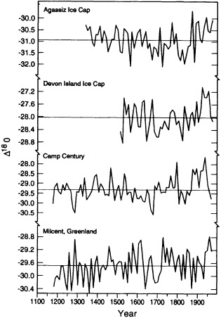
FIGURE 9
Decadal-mean values of d18O ratios from different polar-region ice cores. (See text for details.)
temperatures and water vapor obtained with tropical radiosondes for the past couple of decades have been documented by Flohn et al. (1992), although the drift toward less negative d18O ratios appears to have begun earlier in the ice-core record than in the instrumental climate record.
Changes in interdecadal variability are summarized in Table 2 (see indices 1-4 and 14-15). There is a suggestion that decade-to-decade changes in d18O ratios have increased in amplitude at most of these sites. In particular, the calculated interdecadal d18O variability at Quelccaya has increased sharply in the last 100 years. This increase is evident even though the greater number of samples in the upper part of the record permitted better averages to be created for the recent decades than for earlier periods. A similar signal is apparent on the Dunde ice cap as well. These changes, however, may reflect a more localized temperature signal, changes in moisture sources for snowfall on the ice caps, or some other unknown cause unrelated to climate. It should also be noted that these two sites are located at very high elevations, and thus differ from most of the other
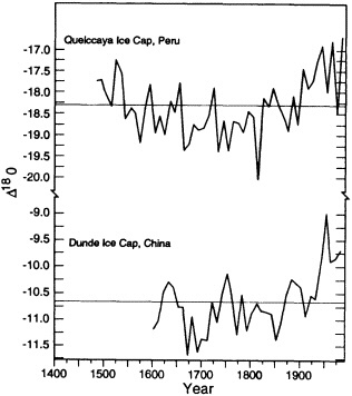
FIGURE 10
The same as Figure 9, but for two tropical ice cores (Quelccaya ice cap, Peru, and Dunde ice cap. China).
paleoclimate indices, which are derived from locations at much lower elevations.
Central England Temperature
Decadal means of winter (December-to-January) and summer (June-to-August) mean temperature for central England (Manley, 1974, and subsequent updates) from 1700 to present are shown in Figure 11. The recent decades do not appear to be exceptional in comparison with the total record. The variability curves (not shown) indicate little overall change, with a tendency for the summer and winter seasons to have opposite changes in interdecadal variability (when one increases, the other tends to decrease). Jones and Bradley (1992, their Figure 13.1) have compared the central England temperature record with 12 other long-period station records in Eurasia and North America. Although there are obvious differences among the various climatic series, the twentieth century does not stand out as being a period of higher decadal-scale temperature variability. Most records (although not all) do exhibit the general warming trend of the past two centuries that is associated with the rebound from the Little Ice Age (see Bradley and Jones, 1992).
SUMMARY AND CONCLUSIONS
The purpose of this study was to evaluate whether the climate in recent decades was ''changing," both with regard
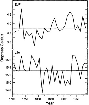
FIGURE 11
Decadal-mean values of central England winter and summer temperature (in °C).
to its mean value as well as with respect to changes in the variance on different time scales. Our findings are mostly mixed, in that the answer depends on the spatial scales selected for analysis.
For the period encompassing the last 100 years, changes in surface air temperature have been greatest and most positive in the period 1970 to 1990. Interannual variability at the largest spatial scales has also increased, although with seasonal differences. By and large, however, increases in variability at these spatial scales are not unique. When one considers smaller regions (in particular different portions of the contiguous United States) the picture changes, so that the 1980s do not necessarily show up as being a unique period in the instrumental climate history of the country.
In order to have a longer perspective on climatic variations, we utilized data from several paleoclimatic reconstructions of growing-season temperature based on tree-ring records and on d18O ratios extracted from different ice-core records. Data from the latter were also taken as a measure of the prevailing air temperature. Annual values were averaged by calendar decades in order to focus on lower-frequency climatic variability. With the exception of the tropical ice cores, the recent decades were not generally unique, in terms of either the average values or increased variability. We note that tropical sea surface temperatures have been generally above the long-term mean since the mid-1970s. It seems plausible that this recent warmth would be reflected in low (less depleted) d18O ratios on the Quelccaya and Dunde ice caps, although more positive d18O ratios were already evident by the 1950s. It should be emphasized again that the exact relationship between actual past climate and these two high-elevation tropical indices is not fully known. Certainly, the period encompassed by the Little Ice Age is reflected in relatively low d18O values, particularly in the Quelccaya record. The development of additional independent ice-core sequences from the Cordillera Blanca in Peru and from extreme western China by L. G. Thompson and colleagues should help in the interpretation of the nature of the climate signals present in these records (e.g., Thompson et al., 1995).
Do we have an answer to the question posed by the title of this study, namely, whether the climate of the twentieth century is different from that of previous centuries? Obviously, the response is not an unequivocal "yes" or "no." As in most instances when one deals with climatic time series, the answer is "It depends." There appear to be differences in regional responses, and they are evident in both the proxy and the instrumental climate records. Insofar as the United States is concerned, the most unusual decade of the last 100 years may have been the 1930s, although the recent period is probably a close second. We can only say that, for most areas of the coterminous United States, the climate of the most recent decades cannot be considered unique, even in the context of the last century.
Commentary on the Paper of Diaz and Bradley
EUGENE M. RASMUSSON
University of Maryland
When Drs. Diaz and Bradley present a paper, it always provides an enormous amount of information. The central question, in terms of a synthesis of the wealth of information provided in this paper, is the question posed by the title: "How different is the climate of the twentieth century"—more specifically the past few decades—"from that of earlier centuries?" In addressing this question the authors examined temperature, decade-to-decade temperature changes, and changes in interannual and interdecadal variability on various spatial scales.
The problem in any analysis of this type, of course, is that of inadequate data distribution in time and space. Thus, the analysis was largely limited to the land areas of the Northern Hemisphere, where both instrumental and proxy data are most plentiful.
It may be well to note that changes in the spatial distribution of observations from decade to decade may affect both the computed area average and the variability. Figure 10 in my paper, which appears later, illustrates the effects of using different data distributions in synthesizing global averages of SST, where the problem is probably more severe than it is over the land areas.
Figure 1 in this commentary also shows estimates of the variability in SST obtained from two different analysis schemes. Two estimates of variability are obtained. One is from the optimal averaging (OA) analysis technique of Vinnikov et al., and I think Dr. Groisman will tell us about that one. Another is derived from the simple box average that has been used—for example, by the U.K. Meteorological Office—in deriving SST area averages. The curves in Figure 10 of my paper show the low-frequency variations, i.e., periods longer than 30 years. There are some differences, but they are not too great, about 0.15 degrees around 1910 and 1920, with the OA staying a little bit closer to the mean for the entire period. Now, if we remove the low-frequency variations so that only the variations on time scales less than 30 years remain (Figure 1 in this commentary), and look at that difference between the two analysis schemes, we see that the level of higher-frequency variability may also depend on the first guess used. The box method and the OA with the previous month as the first guess are similar, but the OA with climatology as a first guess shows less variability during the earlier decades of the series. Thus, relative to the box method, the OA shows an increasing variability with time. This comparison illustrates that one
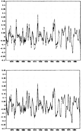
FIGURE 1
Time series of high-frequency variability (periods less than 30 years) of globally averaged sea-surface temperature. Top panel: Dashed curve is obtained by box method (Bottomley et al., 1990). Solid curve is obtained from optimal averaging using climatology as a first guess (Vinnikov et al., 1990). Bottom panel: Curves derived as above except that optimal averaging is obtained by using previous month as the first guess.
must be a bit careful in deriving conclusions about changes in variability from area averages. The estimates of variability may be sensitive to changes in data distribution and the particular analysis scheme used.
Data limitations become extremely severe when one attempts to quantify natural variability on decade-to-century time scales from proxy records. What information can we really derive regarding the patterns of large-scale variability from widely scattered proxy measurements? I think that further effort is required in two areas to maximize and better quantify the information content of the entire climate data base, both instrumental and proxy. First, we need more studies along the lines of data system tests. More specifically, using the more dense data distribution of recent decades, we should determine the loss of information as the distribution of observations is decreased. This will help establish confidence limits for estimates of large-scale averages based on the sparse distribution of observations and proxy series obtained during earlier decades and centuries.
Second, we need to place more emphasis on integration of information from various proxy sources, with the goal of obtaining a better picture of the pattern of global variability during earlier centuries. This is admittedly a formidable task when one is dealing with decade-to-century time scales. I do not believe that the concept of an overall integration of information in decade-to-century variations has yet to take root in the proxy community, but I think it should be strongly encouraged as a long-term goal.
Discussion
GROISMAN: Two quick comments, one for Gene and one for Henry. Gene, I just wanted to note that the SST variability does not reflect conditions over the Arctic. There is about a 25 percent difference in amplitude between SST and marine air temperature over the open ocean, the latter being higher, so there may be other reasons for the difference you cite. Henry, the problem with tree rings is that there are very few 1000-year-old trees, so in a time series you can't resolve the same mean variance.
DIAZ: I used only air temperature over land, no SSTs. Also, I started in 1891, when we had fairly good coverage. The changes in data distribution don't have much influence on the large-scale averages. As for the tree rings, we did try to compensate by looking at decadal means and interdecadal variability, and I don't think the middle section has much of a problem.
KEELING: I have a figure that is based on the Jones-Wigley temperature record, with a slightly different smoothing. Some of the early variability and the apparent biennial signal are probably the result of sparse data; beginning in 1951 the record is fairly homogeneous. You can see the 1958, 1961, 1963, 1982 El Niños. I'd like to know whether there is some difference in the quantity of data, or in its processing now that satellite data and ground data are being mixed, that has changed data variability in the last decade.
TRENBERTH: Perhaps when you fit the spline you are taking out more of the variance at the end.
GHIL: Henry, I was puzzled by the apparently much higher interdecadal variability in the second of your first two tree-ring figures.
JONES: It's partly due to the indexing procedure that there is more low-frequency variance in the top curve than the bottom one, though some of it could be real. KARL: It's important to remember that there are many different ways to classify variability. I suspect that I could show more or less of it just by defining it differently. On this particular figure, I think we need to be aware that one is for a longer season than the other, and the shorter period of a time series will give you higher variability.
DIAZ: Another point is that getting longer time series from proxy records may not improve our understanding of climate change mechanisms.
GROOTES: I want to comment on the Quelccaya ice-core records you used. As you go down from the surface, the seasonal cycle disappears. It reappears about 1880 and continues significant to about 1480. Apparently when there are low values the record is smoothed so little that the seasonal cycle is preserved. As temperature changes it becomes more difficult to calibrate the isotope changes; you may be looking at post-depositional changes rather than the signal itself. Tree rings and ice cores both require particular attention to understanding exactly what you're recording, especially if you are talking about temperature.
MYSAK: For anyone who's interested, I'd like to mention that Brian Luckman at the University of Western Ontario has tree-ring records from the Canadian Rockies for about the last thousand years. He's showing a nice cycle of 150 years or so.
MCGOWAN: Are you comparing tree rings taken from similar altitudes at those different locations? Also, how does the variance of instrumentally measured mountain temperatures compare with that of lowland temperatures?
DIAZ: Most of the data sets are from moderate elevations. As for the high/low elevation temperature variances, the trends are reduced with respect to surface, but they're still comparable.
Variability of African Rainfall on Interannual and Decadal Time Scales
SHARON E. NICHOLSON1
ABSTRACT
This paper examines the rainfall fluctuations that have occurred over the continent of Africa during the past century. Major characteristics include anomaly patterns that are continental in scale, with marked teleconnections between particular sectors of the continent, and quasi-periodic fluctuations with dominant time scales of approximately 2.3, 3.5, and 5 to 6 years. In the Sahelian regions these higher-frequency fluctuations are not apparent; instead, most of the variance is found on time scales of 7 years or longer. Both dry and wet episodes tend to persist for one or two decades at a time; decadal means change by a factor of 2. These characteristics are also apparent in the Sahelian climate record for earlier centuries. Elsewhere on the continent, synchronous changes of rainfall occur, but the "wet" or "dry" decades are not as uniformly wet or dry as in the Sahel. Examples are the 1950s, in which above-average rainfall prevailed over most of the continent, and the 1980s, during which most of the continent was abnormally dry. It is likely that the factors producing higher-frequency interannual variability differ from those producing the decadal-scale fluctuations. Both sea surface temperature and land-surface feedback have been suggested as causes of the unusual persistence in the Sahel, but the latter cannot explain the change of decadal means.
INTRODUCTION
The continent of Africa is primarily tropical or subtropical, so the climatic changes that have taken place have been manifested principally in the rainfall regime. The rainfall fluctuations that occur are extreme; those in the semi-arid regions are probably unmatched anywhere in their magnitude and spatial extent. In the Sahel, for example, decadal averages change by a factor of 2 or more. Most major periods of anomalous rainfall, either individual years or decadal-scale episodes, affect most of the continent.
This paper examines the rainfall fluctuations that have occurred during the twentieth century and compares them with historical episodes. The time scales of the fluctuations are summarized, and the decadal-scale fluctuations described in greater detail. The intra-continental teleconnections, and teleconnections to tropical or global rainfall anomalies, are also considered. Finally, a brief review of causal mechanisms is provided.
Undoubtedly, changes in the thermal regime over Africa have occurred, especially along the continent's poleward
extremes and at higher elevations. These are minor compared to rainfall fluctuations; moreover, they have not been systematically studied. Therefore, this paper will be limited to variability of rainfall.
METHODOLOGY
Most of the description of rainfall variability in this paper derives from previous studies made by the author. Analyses are based on a network (Figure 1) of approximately 1400 stations, the statistics of which are fully described in Nicholson et al. (1988). From these, a spatially averaged data set has been derived, utilizing 90 geographical regions (Figure 1) that are homogeneous with respect to the interannual variability of rainfall.
Regional averages are generally expressed as a standardized annual departure from the long-term mean (i.e., the mean over the entire length of record). In select analyses, the rainfall anomalies are also presented as a percentage departure from the long-term mean. About 75 percent of the station records commence before 1925 and continue to 1984 or later. Hence, the length of record is generally at least 60 years.
Regionally averaged rainfall Rj is calculated as
where Rj is the regional rainfall departure in the year j, and Ij is the number of stations available in year j. In the above, xij is a standardized rainfall departure at station i in
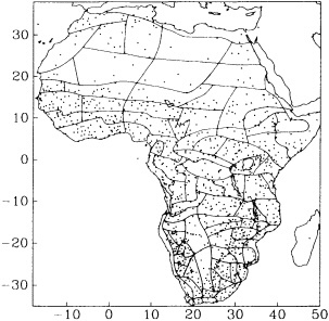
FIGURE 1
Map of rainfall stations in African archive and homogeneous rainfall regions. (From Nicholson et al., 1988.)
year j. It is calculated as
where rij is the annual total at the station in the year j, ![]() is the station's long-term annual mean, and si is the variance of annual rainfall at the station.
is the station's long-term annual mean, and si is the variance of annual rainfall at the station.
These regional means are utilized to examine the temporal and spatial structure of rainfall variability over the continent. They also illustrate the magnitude of decadal anomalies. In some analyses 1°-grid averages are utilized instead of the regional averages.
CONTINENTAL-SCALE PATTERNS OF RAINFALL VARIABILITY
Previous studies (e.g., Nicholson, 1986) have utilized a map-classification technique of Lund (1963) to describe the preferred spatial configurations of rainfall anomalies over Africa. This technique is based on linear correlation of map patterns. Most of the rainfall variability over the continent is described by the six "anomaly types" illustrated in Figure 2. Unlike eigenvector techniques, the patterns produced by the Lund method are not orthogonal; hence, these six anomaly types really describe only four basic configurations of anomalies. These include a tendency for above(or below-) average rainfall over most of the continent (Types 2 and 4) and two patterns (Types 1, 3, 5, and 6) illustrating an opposition between equatorial and subtropical latitudes. Approximately 21 of the 90 years between 1901 and 1990 are represented by a pattern of above-average rainfall in the equatorial regions but below-average rainfall in subtropical latitudes, and 12 by the opposite pattern, which is illustrated by Type 3 in Figure 2. Fourteen of the 70 years are best represented by the Type 2 anomaly pattern, with below-average rainfall throughout most of the continent, and 15 by Type 4, with above-average rainfall in most areas.
These patterns are introduced here for two reasons. First, as will later be seen, they are typical of decadal-scale rainfall fluctuations over Africa. Second, they demonstrate that much of the rainfall variability over the continent can be described using a small number of regional time series. The representative regions, shown in Figure 3, include five latitudinal zones running from the southern margin of the Sahara to the Guinea Coast of the Atlantic, eastern equatorial Africa, and two sectors of southern Africa loosely termed the northern and southern Kalahari.
DECADAL-SCALE FLUCTUATIONS
Fluctuations During Recent Decades
Two major, decadal-scale rainfall anomalies have affected the African continent within the current century:
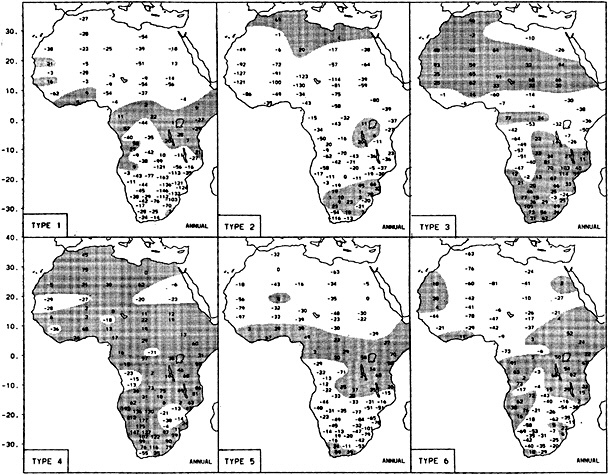
FIGURE 2
The most frequently occurring continental-scale rainfall anomaly types for the twentieth century. (From Nicholson, 1986; reprinted with permission of the American Meteorological Society.) The values represent regionally averaged standardized departures.
TABLE 1 Rainfall Anomalies for the Decade 1980-1989
|
|
1950-1959 Depart.* (%) |
Stdzd. Depart. (% s) |
1970-1979 Depart. (%) |
Stdzd. Depart. (% s) |
1980-1989 Depart. (%) |
Stdzd. Depart. (%s) |
|
Northern Sahel |
37 |
54 |
-31 |
-47 |
-24 |
-35 |
|
Central Sahel |
28 |
71 |
-22 |
-55 |
-31 |
-82 |
|
Southern Sahel |
15 |
62 |
-13 |
-53 |
-20 |
-85 |
|
Soudano-Guinean Zone |
3 |
22 |
-5 |
-36 |
-8 |
-56 |
|
Guinea Coast |
3 |
15 |
-6 |
-31 |
-7 |
-35 |
|
Eastern Africa |
-2 |
-9 |
0 |
4 |
2 |
15 |
|
Northern Kalahari |
8 |
28 |
6 |
20 |
-5 |
-21 |
|
Southern Kalahari |
7 |
23 |
10 |
34 |
-7 |
-27 |
|
* Anomalies are expressed as a percentage departure from the long-term mean and as a standardized departure (ratio of the departure from the mean to the standard departure). |
||||||
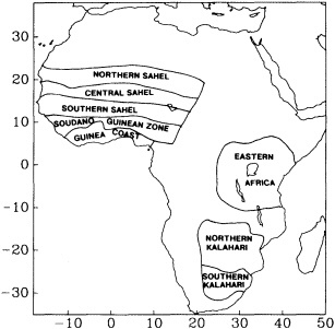
FIGURE 3
Geographical regions described in detail in this study.
relatively wet conditions in the 1950s and relatively arid conditions in the 1980s. The periods of anomalous conditions have not been precisely 10 years in length, nor have they commenced at the onset of each numeric decade (e.g., 1950 or 1960). Nevertheless, these periods and the transition between them are well illustrated from decadal maps and tabulations (Figure 4 and Table 1).
Fluctuations have been particularly large in Sahelian West Africa, where rainfall was about twice as great during the 1950s as during recent years (Table 1). The 1950s (Figure 4a) were also wetter than average over most of the rest of the continent, but abnormally dry in the equatorial regions. The wet episode ended abruptly in the Sahel toward 1960, after which time a change occurred in many other regions.
In the early 1960s, phenomenally wet years occurred in equatorial regions, especially in eastern Africa, while droughts affected much of southern Africa. As an example, Wajir, in northern Kenya with mean annual rainfall of 285 mm, received 612 mm in November 1961; at many Kenyan stations, rainfall that month was five to ten times the long-term mean. The levels of Lake Victoria and other Rift Valley lakes suddenly rose several meters commencing in 1961, abruptly attaining levels unmatched since the end of the nineteenth century. The 1960s as a whole (Figure 4b) was a period of relatively wet conditions throughout the equatorial latitudes and abnormally dry conditions throughout most of the subtropics of both hemispheres. The dry anomaly was particularly strong in the Southern Hemisphere.
The early 1970s were a period of drought over much of Africa (Nicholson, 1986), but later in the decade a series of tremendously wet years occurred in southern Africa, so that for the decade as a whole, a strong opposition is apparent between the two hemispheres (Figure 4c). This is not a common configuration of anomalies, and had previously occurred in only a few isolated years. A plausible explanation is presented below.
The 1980s (Figure 4d), in strong contrast to the 1950s and unlike other decades, was a period of abnormally dry conditions over most of the continent, including most equatorial regions. The decadal anomalies are largest in the Sahel, on the order of + 25 percent in the 1950s and -30 percent in the 1980s (or nearly one standard deviation). In most other areas the departures for the 1950s (Nicholson, 1989) and 1980s (Table 2) are less than 10 percent of the mean.
The continental scale of these anomalies and the abrupt change around 1971 are evident in Figure 5, which shows the linear correlation of the rainfall anomaly pattern of each year since 1901 with anomaly Type 2 in Figure 2. This anomaly type is one of negative departures throughout the continent. Most years from 1950 to 1970 are negatively correlated with it; correlations for 1950-1957, 1961, and 1962 are significant at the 99 percent level. In contrast, nearly every year since 1970 is positively and, in most cases, significantly correlated with the Type 2 pattern.
Teleconnections and Other Characteristics of Rainfall Variability: Comparison of Modern and Historical Periods
The previous section identified several characteristics of African rainfall variability on decadal-scales. One is the tendency of anomalous conditions to persist for roughly a decade. Another is the large magnitude of anomalies in the Sahel. A third is the teleconnections within Africa on decadal-scales, as illustrated by the anomaly types of Figure 2 and the decadal patterns for the 1950s and 1980s (Figures
TABLE 2 Mean Annual Rainfall (mm) at Select Sahelian Stations for Two Recent Periods
|
|
1950-59 |
1970-84 |
|
Bilma |
20 |
9 |
|
Atbara |
92 |
54 |
|
Nouakchott |
172 |
51 |
|
Khartoum |
178 |
116 |
|
Agadez |
210 |
97 |
|
Timbuktu |
241 |
147 |
|
Nema |
381 |
210 |
|
Dakar |
609 |
308 |
|
Banjul |
1409 |
791 |
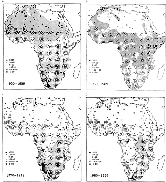
FIGURE 4
Mean rainfall for the periods 1950-1959, 1960-1969, 1970-1979, and 1980-1989 (panels a through d respectively). Rainfall is expressed as a percentage departure from the long-term mean (i.e., the mean for the entire length of record, commencing in 1901 or as soon thereafter as rainfall observations begin). Station data are averaged over 1° squares to facilitate presentation. Shading highlights regions with positive anomalies. (The 1970-1979 map is reprinted from Nicholson, 1994, with permission of Arnold, of the Hodder Headline Group; the 1980-1989 map is reprinted from Nicholson, 1993, with permission of the American Meteorological Society.)
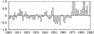
FIGURE 5
Correlation coefficient between the anomaly pattern of each year's rainfall (averaged over the regions shown in Figure 1) and the anomaly pattern corresponding to Type 2 in Figure 2. For the 99 percent confidence level, r ranges from about 0.28 to 0.31, depending in part on the number of regions with available data in a given year.
4a and 4d). Overall, the decadal rainfall fluctuations tend to occur quasi-synchronously over the continent. There is a strong tendency for the fluctuations in the subtropical latitudes of both hemispheres to be roughly in phase, as well as a tendency for the fluctuations in the equatorial and subtropical latitudes to be opposed to each other. These same characteristics are evident in the historical past.
Figures 4a and 4d clearly demonstrate that major periods of anomalous rainfall in the Sahel correspond to continental-scale anomalies as well. This is likewise true for historical fluctuations of Sahel rainfall, such as the droughts of the 1820s and 1830s and the 1910s (Figure 6). Both of these periods were times of frequent drought throughout much of the continent. A period of sufficient rainfall from about 1870 to 1895 was part of a continental pattern mirrored by the 1950s pattern (Figure 4a). In the 1950s, lake levels rose dramatically from Chad in the north to Ngami in the south, and the floods of rivers like the Niger and Nile were consistently high. Near Timbuktu, in the Niger Delta where annual rainfall is now 195 mm, wheat production thrived to such an extent that grain was exported to neighboring regions. In the semi-arid regions of North Africa rainfall probably averaged about 25 to 30 percent above the twentieth-century mean during the period 1870-1895 (Nicholson, 1978).
Interestingly, the historical patterns depicted in Figure 6 were constructed prior to the derivation of the rainfall anomaly types in Figure 2; they were based on proxy data and qualitative indicators. While this origin might render the reconstructions questionable, their reliability is supported by the clear correspondence to the major anomaly types apparent in the modern quantitative rainfall record. They also demonstrate other major characteristics of African rainfall variability established with modern records: the decadal-scale persistence of anomalies in the Sahel, and their continental scale.
In certain cases, global teleconnections to decadal-scale African rainfall fluctuations have also been demonstrated. One example is the change from "wetter" to "drier" conditions around the turn of the century. This change was seen throughout the tropics, with a major shift occurring around 1895 (see, e.g., Kraus, 1955a,b). The anomalously dry 1830s was also a period of globally anomalous climate, often considered to mark the end of the Little Ice Age. The anomalous conditions of the 1950s are also noted in other tropical and subtropical regions such as Central America, India, and Australia. These decadal teleconnections have not, however, been studied systematically.
Fluctuations on Time Scales of Centuries
The climatic fluctuations that have affected Africa on time scales of centuries are difficult to establish because
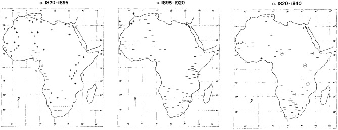
FIGURE 6
African rainfall anomalies for three historical periods. Minus signs denote evidence of drier conditions; plus signs denote evidence of above-average rainfall; zeroes denote near-normal conditions; circled symbols denote regional integrators, such as lakes or rivers. (From Nicholson, 1978; reprinted with permission of Academic Press Ltd.)
there are few long-term climate data sets or even proxy records from which past climatic conditions can be reconstructed. Two notable exceptions are Lake Chad, the fluctuations of which have been well documented through both historical and geological methodologies (Maley, 1976), and the Nile, for which quasi-continuous written records extend back to the seventh century (Toussoun, 1923; Riehl et al., 1979). However, neither record lends itself to completely unambiguous interpretation.
The Lake Chad record suggests two long periods of comparatively wet conditions in the West African Sahel, one in the ninth through fourteenth centuries and another from the sixteenth through nineteenth centuries. The first was synchronous with the Medieval Warm epoch and the second occurred more or less during the Little Ice Age of Europe. The more humid climates in the present-day Sahel, which the Lake Chad record implies, are further supported by numerous historical and geological indicators throughout West Africa. Information for other regions of Africa is more scarce, but the Nile record and those of other East African lakes suggest that the first humid period affected much of eastern equatorial Africa as well. The second appears to have affected that region and much of southern Africa (Nicholson, 1979a, 1981). The decline of the recent wetter conditions took place toward 1800, at a time when the Northern Hemisphere was experiencing the end of the Little Ice Age.
INTERANNUAL VARIABILITY OF RAINFALL
Because of the limited availability of meteorological data for time scales of 10 to 100 years, it may be necessary to evaluate mechanisms of variability on these time scales at least partially through analogy with individual years. For this reason, a description of the interannual variability of African rainfall is relevant here. This section examines the temporal characteristics of rainfall variability in various regions in the domains of both time and frequency. Several of the features exhibited will have to be adequately accounted for by any mechanism that is proposed as explaining variability on 10- to 100-year time scales.
Figures 7 and 8 show the standardized rainfall departure series for select regions of Africa. The most striking feature in any of the series is the extreme persistence of rainfall anomalies in Sahelian West Africa (Figure 7). This persistence was first identified by Bunting et al. (1976), then later by Walker and Rowntree (1977), Nicholson (1979b, 1983), and Lamb (1982). In the Sahel as a whole (a combined series of northern, southern, and central Sahel in Figure 7), regionally averaged rainfall exceeded the long-term mean in every year from 1950 to 1967; it has been below the mean in every year since 1970. Rainfall also tended to be above average throughout most of the period 1927 through 1936 and below average in the 1910s and 1940s. To some
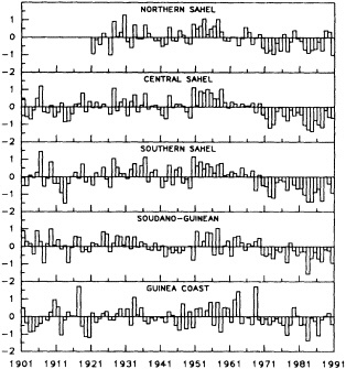
FIGURE 7
Rainfall fluctuations in West and North Africa (1901 to 1990), expressed as a regionally averaged standard departure. Location of the regions is indicated in Figure 2.
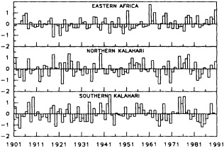
degree, this persistence is also apparent in the Soudano-Guinean and Guinean regions further south.
Such long-term persistence is not evident in any of the other regional time series. For example, the longest run of ''dry" years is 5 years in the northern Kalahari, 6 years in the southern Kalahari, and only 3 years in eastern Africa (Figure 8). The longest run of "wet" years is 5 years in all three regions. However, longer periods of predominantly wet or dry years have prevailed. These include, for example, the "dry" 1950s in East Africa and the drier periods of 1926 to 1935, the 1960s, and the 1980s in the southern Kalahari.
The contrast between the Sahelo-Saharan region and elsewhere in Africa is underscored by Figure 9. It shows the results of low-pass filtering the rainfall series for the regions in Figure 1 and isolating the percentages of variance of annual rainfall on time scales longer than 7 years. This variance represents a combination of decadal-scale or longer fluctuations and year-to-year persistence of rainfall anomalies. Low-frequency variance is by far the greatest in the Sahelian regions, accounting for as much as 45 to 60 percent of the variance. Elsewhere it is generally between 20 and 35 percent.
Spectral analysis shows that the dominant time scales of rainfall variability throughout the continent are on the order of 2.2 to 2.4, 3.3 to 3.8, and 5 to 6 years (Rodhe and Virji, 1976; Ogallo, 1979; Nicholson and Entekhabi, 1986). These are not the only periodicities that have been detected, but they are the only ones apparent throughout large expanses of the continent and the only ones corresponding to time scales of distinct causal mechanisms such as SST fluctuations or ENSO. The works of Tyson (e.g., 1980), Fleer (1981), and others provide more detail on select regions.
The occurrence of these quasi-periodicities in the regions depicted in Figure 1 were evaluated by Nicholson and Entekhabi (1986). The results are shown in Figure 10. The 5- to 6-year time scale is dominant in equatorial regions; the 3.5-year time scale is dominant in much of southern Africa and in parts of equatorial Africa; the 2.3-year time scale is dominant in the eastern half of equatorial and south-
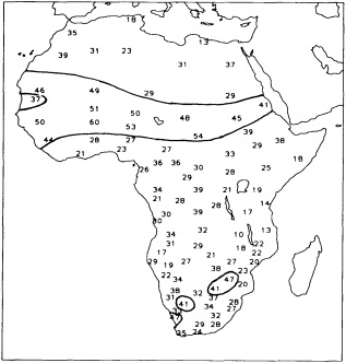
FIGURE 9
Percentage variance of annual rainfall with periods of 7 years or longer for regions depicted in Figure 1 (in circled areas, variance exceeds 40 percent).
ern Africa. Interestingly, these relatively high-frequency fluctuations (Figure 10) are nearly absent throughout the Sahelo-Saharan region of West Africa, where the spectra are dominated by low-frequency fluctuations (Figure 9). Relatively low-frequency fluctuations have been noted also in parts of South Africa (Tyson, 1980), with time scales of 18 to 22 years being common.
An examination of wet and dry years throughout the continent (e.g., Nicholson et al., 1988) shows other characteristics of interannual variability that must be explained. One is that in many regions interannual variability is associated not with a change in the intensity of the rainy season but by a change in the length of the season or by anomalous rainfall in comparatively dry months. This can be demonstrated for East Africa as well. Throughout most of the region, the main rainy season is April to May, but interannual variability is best correlated with anomalies of the "short rains" of October-November (Figures 11 and 12). The importance of transition-season fluctuations also helps to explain the rainfall's continental-scale coherence over regions (such as the African Northern and Southern Hemispheres) where the rainy seasons are six months out of phase.
Rainfall in East Africa illustrates another interesting characteristic: The factors that produce the climatological-mean
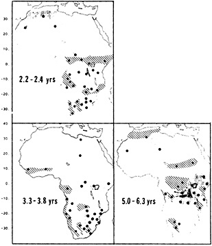
FIGURE 10
Distribution of significant spectral peaks with periods on the order of 2.2-2.4, 3.3-3.8, and 5-6 years. Data are for regions shown in Figure 1, with blanks indicating no significant peak in the regional rainfall. (From Nicholson and Entekhabi, 1986; reprinted with permission of Springer-Verlag.)
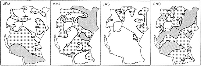
FIGURE 11
Correlation between the seasonal and annual rainfall departure series for East Africa (representing the countries Kenya, Uganda, and Tanzania). Values approximately equal the percentage variance explained by each season: stippling, 50 to 70 percent; shading, greater than 70 percent.
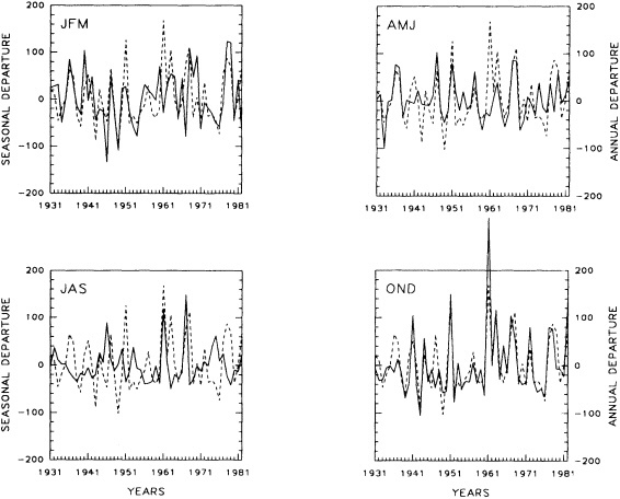
FIGURE 12
Time series of rainfall departures for individual seasons (solid line) compared with the annual rainfall departure series representing East Africa (Kenya, Uganda, and Tanzania). Data are expressed as a percentage standard departure.
patterns are not necessarily those that explain interannual variability. Within this region, mean annual rainfall and its seasonality are highly heterogeneous (Figure 13), being associated with several features of the general atmospheric circulation as well as with regional-scale orographic and lacustrine effects. Nevertheless, the patterns of interannual variability are markedly similar throughout the region (Figure 14), so that there is a remarkable resemblance between the time series for the region as a whole, and for those four climatologically homogeneous subregions. The first eigenvector of annual rainfall shows loadings of the same sign throughout the region; the pattern explains 36 percent of the variability of annual rainfall and 52 percent of the variability during the "short rains" (Nyenzi, 1988).
In summary, there are several notable characteristics of rainfall variability that must be explained by mechanisms for producing this variability. These include, first of all, the continental-scale coherence and the seemingly contradictory contrast between the dominant low-frequency fluctuations in Sahelo-Saharan regions and the high-frequency fluctuations elsewhere, in regions that show strong teleconnections to the Sahel on time scales of 1, 10, and 100 years. The characteristic time scales of 2.3, 3.5, and 5 to 6 years must likewise be explained, as must be the seasonality of the changes and the coherent patterns of interannual variability in climatically heterogeneous regions.
MECHANISMS OF RAINFALL VARIABILITY
Most studies of African rainfall have focused on interannual variability. Numerous authors have demonstrated relationships between SSTs and rainfall in various parts of Africa (e.g., Lamb, 1978; Lough, 1986; Semazzi et al., 1988; Wolter, 1989; Folland et al., 1991; Nicholson and Entekhabi, 1987). For parts of eastern and southern Africa linkages to ENSO have also been clearly established (by, e.g., Farmer, 1988; Ropelewski and Halpert, 1987; Ogallo, 1987; Harrison, 1983; Lindesay et al., 1986; Nicholson and Entekhabi, 1986, 1987). For Sahel rainfall, a number of other factors, such as changes in the upper-level winds and in the Hadley and Walker circulations, have also been implicated (Kanamitsu and Krishnamurti, 1978; Newell and Kidson, 1984).
Very little attention has been paid to the causes of the lower-frequency variability. The exception is the work by Folland and collaborators (e.g., Folland et al., 1991), which is limited to the Sahel. Virtually no studies have been carried out on the causes of the continental rainfall fluctuations on decadal time scales.
Rowell et al. (1992, 1995) suggest that the twentieth-century trends in Sahel rainfall can be attributed to interhemispheric differences in sea surface temperature. The interhemispheric contrast increased in mid-century and decreased sharply as the droughts began in the 1970s and 1980s. This mechanism does not, however, account for the extreme persistence of anomalies in the Sahel, or their lack of persistence in regions such as southern Africa, which otherwise appear to have teleconnections to the Sahel in individual years and on decadal-scales.
Land-Surface Feedback in the Sahel
As an example of how this might work, consider a year during which anomalous large-scale circulation triggers drought in the Sahel and in other African regions showing strong teleconnections to the Sahel. When the large-scale forcing returns to normal, so do rainfall conditions in most areas. However, in the Sahel the drought conditions might be reinforced by local, land-surface feedback. In that case they will persist until a year in which a large-scale circula-

FIGURE 13
Maps of rainfall characteristics over East Africa: mean annual rainfall, number of rainfall maxima in the seasonal cycle, and the months of these maxima. (From Nicholson et al., 1988.)
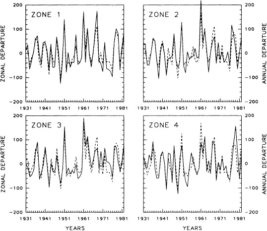
FIGURE 14
Time series of rainfall departures for the four regions shown in the inset map (solid lines) compared to the time series for East Africa as a whole (dashed lines). Values are expressed as a percentage standard departure from the long-term mean.
tion anomaly occurs that is sufficiently great to override that local forcing.
In southern Africa, a region with rainfall teleconnections to the Sahel (see above) but without strong interannual persistence of rainfall anomalies, the interannual variability of surface fluxes is smaller and less spatially coherent. The rain-bearing systems in that region are also less sensitive to surface processes than are those affecting the Sahel.
This might suggest the following hypothetical scenario for explaining the unusual pattern of the 1970s: below-normal rainfall in Sahelo-Saharan regions and above-normal rainfall in corresponding sectors of Southern Hemisphere Africa. The factors producing drought commencing in 1968 were reinforced in the Sahel by land-atmosphere interaction that caused the negative anomalies to persist without interruption throughout the 1970s. In the mid-to-late 1970s, some factors in the general atmospheric circulation produced wet conditions in southern Africa and also enhanced rainfall in Sahelo-Saharan regions. In the latter, however, they were insufficient to override the drought-promoting feedback and resulted in less extreme negative anomalies in years such as 1974 to 1978, but not in rainfall exceeding the long-term mean.
It is interesting to note that when only high-frequency fluctuations are considered, the rainfall fluctuations in the Sahel bear a much stronger similarity to those in the Kalahari (Figure 15) during the past 40 years. The correlation between the resulting "Sahelian" series and the rainfall series for the northern Kalahari is 0.5, just slightly lower than the correlation (0.57) between the series for the northern and southern Kalahari in Figure 8.
The results shown in Figure 15 are consistent with the idea that higher-frequency fluctuations, or yearly departures from a decadal or multi-decadal mean, are forced by similar factors in Sahelian and southern Africa. but that additional causal mechanisms of lower-frequency variability must be sought in the Sahel. A similar contrast in forcing is apparent between various parts of the Sahel and between the early
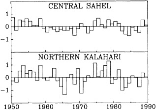
FIGURE 15
Rainfall variations in the Sahel and the Kalahari for the period 1950 to 1990. Rainfall in the Kalahari is a standardized departure from the long-term mean. For the Sahel, standardized departures for 1950 to 1969 are calculated with respect to the mean for that period; those for 1970 to 1990 are calculated with respect to the latter period. For both, the variance is calculated with respect to the entire length of the record. This is roughly equivalent to removing the low-frequency variance from the Sahel series. (From Nicholson, 1993; reprinted with permission of the American Meteorological Society.)
and late rainy-season months. High-frequency forcing is also stronger in June-July than in August-September. This observation is relevant because one hypothesized factor in the feedback, the African Easterly Jet (see below), is operative mainly in the latter period.
The potential feedback mechanisms involve the effect of such factors as soil moisture and dust generation on surface fluxes and atmospheric heating. The dynamic link to the Sahel could be the mid-level African Easterly Jet. The African Easterly Jet is a consequence of the meridional temperature gradient in the region, which in turn is produced by the strong thermal contrast between the dry Sahel-Saharan region and the forests and Atlantic Ocean to the south. It is analogous to the mid-latitude westerly jet stream, in that it provides the instability and energy for the development and maintenance of rain-bearing systems in the Sahel. It has a maximum around 650 or 700 mb, a level where the temperature structure is strongly affected by surface-generated dust. The intensity of the dust, in turn, is highly inversely correlated with rainfall in the Sahel.
The contrast in surface fluxes between wet and dry years (Lare and Nicholson, 1993) is sufficiently large to produce the observed changes of jet intensity between wet and dry years (Newell and Kidson, 1984). These in turn are sufficiently large to influence the jet's dynamics, and are thus capable of altering such variables as the number, size, and intensity of disturbances in the region.
SUMMARY AND CONCLUSIONS
Numerous studies have firmly established that:
-
decadal-scale rainfall fluctuations have been quite marked in Sahelian Africa;
-
these fluctuations tend to have a continental spatial scale (although less extreme and persistent than in the Sahel) with distinct teleconnection patterns;
-
the characteristics of modern decadal anomalies are also apparent in earlier centuries; and
-
the 1950s and, to a lesser extent, 1960s were continentally "wet," while the 1980s and, to a lesser extent, 1970s have been continentally "dry."
Among the major areas in which research is needed are the causes of the decadal-scale fluctuations of African rainfall, particularly the continentally coherent patterns; the role land-surface feedback may play in the decadal-scale anomalies in the Sahel; and the teleconnections between African rainfall anomalies on the decadal-scale and global climate anomalies.
Our understanding of decadal-scale fluctuations could be greatly enhanced by comparative analysis of the 1950s and more recent decades. Unfortunately, many of the necessary data are routinely available only for about the last 20 years. However, a great many data, especially upper-air data, do exist for the 1950s and 1960s, but in obscure archives where they are not readily available. Effort should be devoted to creating usable data sets for earlier periods, especially the 1950s.
Our knowledge of African climate fluctuations on the scale of centuries is considerably more vague. In order to establish these regional fluctuations' causal mechanisms and their relationships to global climate fluctuations, they must be more precisely delineated in time and space. This will require the preparation of better proxy data sets. Few attempts have been made to use, for example, tree-ring or varve chronologies. Also, the innovative paleoclimatic techniques that have been developed recently might be appropriate here as well. Creation of these proxy data sets for Africa should be a high priority.
On the Initiation and Persistence of the Sahel Drought
JAGADISH SHUKLA1
ABSTRACT
On the basis of analysis of data collected over the Sahel, India, and China, it is conjectured that the occurrence of above-normal rainfall over the Sahel during the decade of the 1950s and below-normal rainfall during the decades of the 1970s and 1980s is a manifestation of natural variations in the planetary-scale coupled ocean-land-atmosphere climate system. In the light of the results of general-circulation model sensitivity experiments, and the fact that the Sahel region is particularly susceptible to changes in land-surface conditions, it is concluded that strong local atmosphere-land interactions over the Sahel region have contributed toward further reduction of rainfall. Both natural climate variability and human activities degrade the land surface in a way that exacerbates the ongoing drought, and therefore there is no guarantee that natural variability can reverse the present trend.
INTRODUCTION
The West African famine during the late 1960s and the 1970s focused the world's attention on the Sahel. The Sahel is a 200- to 500-km wide band across the southern reaches of the Sahara desert. It is ecologically fragile, though it supports nomads, herders, and sedentary farmers; it has a mean rainfall of 300 to 500 mm per year, which is extremely variable. During the past 25 years, rainfall over the Sahel has been significantly lower than the long-term mean. In the recorded meteorological data for the past 100 years, there is no other region on the globe of this size for which spatially and seasonally averaged climatic anomalies have shown such persistence. (See the paper by Nicholson in this section.)
In this paper we shall attempt to address the following questions concerning the Sahel drought:
-
What are the causes of the onset of the drought? In particular, what significant roles did the natural variability of the global climate system and of human activities play in the initiation of the drought?
-
What mechanisms are responsible for the persistence of the Sahel drought?
-
What are the prospects for reversal of the current trend? In particular, what roles might the natural variability of the global climate system and human intervention play in reversing the current trend?
It is of course difficult, if not impossible, to give precise
answers to these questions. We will attempt to address them by interpreting past observational data and the results of controlled sensitivity experiments made with general-circulation models (GCMs).
ONSET OF THE SAHEL DROUGHT
Figure 1 shows the 10-year running-mean seasonal rainfall anomalies over Sahel, India, and China. The Chinese rainfall data are available for only a 30-year period (19511980); therefore, the Indian and the Sahel rainfall data have also been shown for that period.
We interpret these data to suggest that the occurrence of above-normal rainfall during the decade of the 1950s and the early 1960s, and below-normal rainfall during the late 1960s and the 1970s, is a feature common to the vast areas of African-Asian monsoon, not one confined to the Sahel region. We do not know why rainfall over such a large geographic region, covering two continents, was above normal during the 1950s. We also do not know why the transition from above-normal to below-normal rainfall that
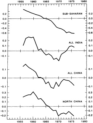
FIGURE 1
Ten-year running mean of normalized rainfall anomalies averaged for all the stations over the sub-Saharan region (10° - 25°N, 18°W - 25°E), India, and China. North China refers to the area to the north of 35°N.
took place during the late 1960s occurred over the entire African-Asian monsoon region. However, on the basis of comprehensive GCM sensitivity studies (Folland et al., 1986; Rowell et al., 1992; Xue and Shukla, 1993), it is now generally accepted that the rainfall anomalies, especially over the Sahel, are consistent with, and can be simulated using, the global sea surface temperature (SST) anomalies during these periods.
On the basis of the GCM sensitivity experiments andobservations shown in Figure 1, we conjecture that the onset of the Sahel's rainfall deficit in the late 1960s, along with the above-normal rainfall in the 1950s, should be explained as a regional manifestation of the planetary-scale variability of the global coupled ocean-land-atmosphere climate system. Considering the large spatial and temporal extent of these rainfall anomalies, we cannot conceive of any possible mechanism by which local human-induced changes could initiate such major droughts over two continents. We therefore reject the notion, often mentioned in popular literature, that the Sahel drought was initiated by human activities.
We believe that the pertinent question about the Sahel drought is not what initiated the drought (we conjecture it was natural variability) but why the drought has persisted for 25 years.
PERSISTENCE OF THE SAHEL DROUGHT
We further propose that strong interaction between atmospheric and land-surface processes is one of the primary causes of the drought's persistence: A reduction in rainfall (due to natural variability of the climate system) would change the land surface characteristics (increase in albedo and decrease in vegetation), which in turn would cause further reduction in rainfall. The basic mechanisms of atmosphere-land coupling have the potential to perpetuate an initial drought (or an initial excessive-rainfall) regime until they are reversed by an opposite forcing, which could be produced by natural variability.
The extent to which changes in the land-surface properties can influence the local climate depends on the spatial scale of the changes in the land-surface characteristics and the geographic location of the region. We submit that the Sahel region is particularly sensitive to atmosphere-land coupling processes. The Sahel region is geographically unique in that it is adjacent to the largest desert on the earth's surface, and it represents the largest contiguous land surface without extensive mountain terrains. The absence of large-scale topographic forcing in the region is perhaps one of the main reasons for the lack of zonal asymmetry in the rainfall pattern there. As Charney (1975) pointed out in his seminal paper on the dynamics of Sahel drought, climate in the subtropical margins of the deserts is particularly vulnerable to changes in the land-surface properties.
During the past 20 years there have been a large number of GCM sensitivity studies (Mintz, 1984; Dirmeyer and Shukla, 1993) that show that increases in albedo and decreases in vegetation cover and soil moisture tend to further reduce rainfall over the Sahel. We do not know of any GCM sensitivity study challenging this basic result. We present here the results of a recent GCM sensitivity study (Xue and Shukla, 1993 and an unpublished manuscript) in which the Center for Ocean-Land-Atmosphere Interactions (COLA) model was integrated with two sets of land-surface conditions over the region south of the Sahara desert. In one set of integrations, referred to as the "desertification" experiment, it was assumed that the area approximately between 10° and 20°N and 15° and 40°E was covered by shrubs above bare soil. In the other set of integrations, referred to as the "reforestation" experiment, the area approximately between 15° and 40°E was covered by broadleaf trees above ground cover. The first set of surface conditions (desertification) was considered to represent the exaggerated state of current conditions. The second set of surface conditions (reforestation) represented a hypothetical situation in which vegetation was maintained in the margins of the Sahara Desert. It was an exaggeration of the conditions during the 1950s, when rainfall over the Sahel was above normal, and the latitude of the 200 mm isoline of seasonal rainfall in the western Sahel was at about 18°N. The model was integrated with identical global SST patterns for each change in the land-surface conditions.
Figure 2a shows the difference between the observed rainfall averaged for 1950 plus 1958 and 1983 plus 1984. Figure 2b shows the difference between the desertification and reforestation experiments for seasonal mean rainfall. The similarity between Figures 2a and 2b is remarkable. Both show negative rainfall departures between 10° and 20°N and a positive rainfall departure to the south of the negative departures. The dipole nature of both the observed and the model rainfall anomalies suggests a southward displacement of the mean rainfall pattern.
Since the only changes in these integrations were those in land-surface conditions, it is reasonable to conjecture that if the natural variability of the global climate system were to produce an initial drought, the strong atmosphere-land interaction over the Sahel region could contribute toward the persistence of that drought.
We further propose that since natural changes in the Sahel rainfall have led to large-scale changes in human activities in the region, it is quite likely that the degradation of the land surface was exacerbated by human activities (overgrazing, deforestation, soil desiccation, etc.), thereby producing further reduction in the Sahel rainfall. The exacerbating effects of human activities could have been especially large during the past 30 years because the population density has been much higher than at the beginning of the century.
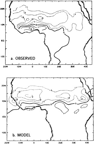
FIGURE 2
(a) Observed summer (June, July, August, September) rainfall difference, in millimeters per day, for the average of 1983 and 1984 minus the average of 1950 and 1958. (b) Rainfall difference between desertification and reforestation GCM experiments.
The various conjectures put forward in this paper so far have been synthesized in a schematic diagram shown in Figure 3. It is seen that the atmosphere-land interaction has a positive feedback mechanism, so that initial drought caused by the natural variability of the climate system is perpetuated by increases in albedo and decreases in vegetation, soil moisture, and surface roughness. In addition, the human-induced effects also produce an increase in albedo and a decrease in vegetation, soil moisture, and surface roughness. Thus, both the planetary-scale effects and the human-induced effects are mutually reinforcing the dry conditions, which has led to an unprecedentedly long and severe drought over the Sahel.
THE FUTURE
If we accept the premise presented in the beginning of this paper, that the Sahel drought was initiated by natural
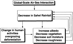
FIGURE 3
Schematic representation of the mechanisms affecting Sahel rainfall. Both the natural variability and the human-induced changes are contributing to the reduction in Sahel rainfall.
variability of the global climate system, it is reasonable to assume that at some unpredictable future time the natural variability (global SST patterns, for example) is likely to produce excessive rainfall over the Sahel and thus reverse the current drought. However, it is unclear whether the changes in the land-surface characteristics can also be reversed. Therefore, even if the global circulation shifts in such a way as to be favorable for reversing the current drought, the global natural changes will have to be stronger than before, and more favorable, to overcome the opposing effects of local atmosphere-land interactions. In fact, it is entirely possible that the Sahel drought will continue indefinitely, because the natural variability effects may never be large enough to counteract the persistent effects of the local land-surface changes.
In a hypothetical GCM sensitivity experiment, Xue and Shukla (unpublished manuscript) have shown that rainfall over the Sahel can be increased by replacing the broadleaf shrubs over ground cover and the shrubs over bare soil by broadleaf trees over ground cover over a large region that includes the Sahel. This suggests that although human effects were not responsible for the initiation of the Sahel drought, a suitable combination of large-scale natural variability and human intervention might contribute toward reversing the current drought. Modification of surface albedo, evapotranspiration, or surface roughness would all be of assistance, though of course it would be extremely difficult to sustain vegetation on a scale sufficiently large to halt the spread of the desert.
Discussion
DESER: Do you think local forcing applies to the string of wet years in the 1950s and 1960s too?
NICHOLSON: Absolutely. What I feel is the critical factor involved in the forcing is the fluxes to the atmosphere, including dust. The land surface forcing should be reversible, or symmetric, for the wet and dry periods.
RIND: How successful have people been in quantifying the albedo change between the wet and dry periods, as far as the land surface is concerned?
NICHOLSON: One study made 10 or 15 years ago took the available satellite data and reconstructed the albedo over about 8 years. The small changes found were not consistent with rainfall fluctuations, and I think basically showed that albedo is not one of the major forcing factors. More recently, Vivian Gornitz searched historical archives for material on land-surface changes, and constructed a beautiful map of West Africa showing changes due to human activities. Again, in terms of absolute values of albedo, it's a very small change, and sometimes in the wrong direction for the Charney mechanism. So I think that not albedo but something coupled to soil moisture, vegetation, and dust will be the major factor.
DIAZ: To what degree do you think that time differences in the frequency of the westward-propagating tropical disturbances affect the variability you're seeing?
NICHOLSON: I think they're key to understanding the region. This may be the one place on the globe where the land-surface forcing per se has a major impact on the overall large-scale dynamics. The jet stream at the mid-levels here, which is critical in disturbance development, is due to nothing other than the temperature gradient across the land surface down to the ocean.
Some of the models done years ago, during the GATE days, showed that if you change the relationship between baroclinic and barotropic instability you can change the characteristics of the disturbances. The difference between the wet 1950s and the dry 1970s can be explained by one or two disturbances a month that produce, say, 150 mm of precipitation a day, where the dry periods have nothing over 50. I think the large-scale circulation is clearly coupled to the land surface there. Incidentally, the dust in that region is right at the level of the African easterly jet, about 650700 mb, which is another reason I think it is so important.
CANE: I can see that the land-surface processes can affect what's happening, but I'd like to hear what you see as the feedback
mechanism for very-long-period changes. How would you cycle in and out, and what would the trigger be?
NICHOLSON: Well, if you assume some large-scale trigger in the general atmospheric circulation, maybe a major change in SST, you could get a continental-scale pattern like the wet 1950s all over Africa. But in other areas the rainfall goes back to normal, whereas in the Sahel the anomalies persist for 10 or even 20 years. There has to be some other smaller-scale forcing that reinforces the existing conditions until it's overridden by some larger trigger in the atmosphere-ocean circulation.
COLE: Ropelewski and Halpert's analysis of global rainfall suggests that the ENSO teleconnection with African rainfall is strongest in the east. Do you see a strong ENSO signal in the variability in the area you've been looking at?
NICHOLSON: There's a small one in the coastal region, but nothing in the central Sahel.
RIND: Shukla, your hypothesis suggests two questions to me. The first is, can it be documented—through satellite observations, for instance—that the vegetation really changed so extremely in those 10° latitude belts? And the second is, did those British experiments in which SST anomalies related so well to the Sahel changes, also produce the drying conditions in China and India between the 1950s and 1980s?
SHUKLA: We have exaggerated the extent of land degradation in our experiments. But there is a very clear shift in the rainfall between the 1950s and the 1980s, and Tucker and his colleagues have shown from the vegetation data that there is a very clear relationship between the two. If you look at the latitude of an isoline, it is definitely going down; the 200-mm isoline has dropped by 2° or 2.5°. So there are changes at the boundary, albeit of less magnitude than what I have chosen for this experiment.
BERGMAN: Sharon, when I was at the Climate Analysis Center, we found amazing discontinuities in precipitation time series in Western Africa that suggested that the station sites for some locations must have been moved, although there was no record of a change. Did you find this, and were you able to correct for it?
NICHOLSON: There were only a couple of stations in my network that had to be thrown out because of that sort of discontinuity, though we did find differences at the same station because of varied sources. Our approach has been to take aerial averages and hope that the outliers get factored out. But let me make a pitch here for the need to put together an archive of some of the old, forgotten data sources, such as pilot balloon data, to help us understand decadal and longer-scale variability.
RASMUSSON: It is still not clear to me that we are seeing the effect of human intervention. The vegetation seems to move north again in wetter years. Can you see an underlying southward trend'?
NICHOLSON: Shukla and I differ somewhat in our views here. I think that so far human intervention has very little to do with it. Many of the papers on desertification are essentially inferring continent-wide desertification from two data points in West Africa. But I don't think that the vegetation's recovery changes any of the ideas about the relation between low-frequency forcing and land surface.
One other thing I'd like to mention with respect to Shukla's argument is that I think one variable has been left out: dust. If I had to put money on any of those land-surface variables, I'd pick dust. It responds to both rainfall and land-surface factors, it has the best memory in the system, and it has shown the most consistent relationship over time with rainfall fluctuations.
SHUKLA: That is certainly a point that ought to be discussed further, if we had time. I'd like to think a little more before I put my money on dust. But let me add just a couple of things. The population pressure has been higher than ever before in the past 20 or 30 years, and that period coincides with the most severe drought in the 100 or so years for which we have reliable instrumental data. Proxy-data evidence of persistent droughts by no means rules out a human role in the current situation. It is also possible that human intervention, such as large-scale agriculture and afforestation, has the potential for reversing the present tendency, whatever its origin.
Continental Snow Cover and Climate Variability
JOHN E. WALSH1
ABSTRACT
In terms of its interactions with the atmosphere, snow cover has received the most attention through the albedo-temperature associations that have been detected over daily to monthly time scales. For example, snow cover has been shown to contribute, albeit modestly, to the interannual variability of monthly surface air temperatures over land. On decadal and longer time scales, the more important role of snow cover may be its link with the hydrologic cycle over land. Changes in winter precipitation and/or temperature can, through snow cover, result in substantial temporal and spatial changes of soil moisture and runoff to the oceans. Model results are rather consistent in depicting an alteration of the seasonal cycle of temperature when the timing and amount of spring snow melt are modified. Runoff-induced effects on the ocean stratification in the middle and high latitudes have also been hypothesized, although such arguments need to be substantiated by observational data. Greenhouse-induced changes of high-latitude precipitation, especially snowfall, play significant roles in the scenarios of temperature change projected by global climate models. Data on observed snow cover and temperature variations of recent decades are, in some respects, consistent with the projections of the global models.
INTRODUCTION
Snow cover has long been regarded as an indicator and as a possible agent of climate variability over a range of time scales. Over periods of several days to several weeks, the largest changes in the earth's surface properties result from variations in snow cover on land and on sea ice. Snow cover clearly influences the local values of near-surface atmospheric variables over these time scales. Over time scales of a thousand years or longer, the advance and retreat of the ice sheets depend ultimately on changes in the rates at which snow accumulates and ablates over the continents. However, over the interannual-to-century time scales on which this workshop will focus, the climatic roles of snow cover are poorly understood. Aside from the areal snow coverage of the past 15 to 20 years, the variability of snow cover over decadal time scales is not well documented. Yet model results are sufficiently suggestive of climatic roles of snow cover that one cannot ignore snow cover in projections of climate change over decade-to-century time scales.
This paper begins with a brief discussion of the physical basis of associations between snow cover and atmospheric variability. Manifestations of these associations in observational data and in model experiments will then be surveyed. While this survey contains several illustrations of shorter-term interactions between snow cover and the atmosphere, the emphasis will be on interactions within the land-atmosphere system over the interannual, decadal, and century time scales. Because sea ice is the focus of another paper in this volume, we limit the discussion to interactions involving snow on land.
PHYSICAL BACKGROUND
A major difficulty in quantifying the climatic role of snow cover is that the distribution of snow is primarily a consequence of the large-scale pattern of atmospheric circulation, which determines the broad features of the distributions of temperature and precipitation over land. Thus, even in the absence of any causal role of snow cover, there can be large statistical correlations between anomalies of snow cover and atmospheric circulation. However, the pattern of atmospheric circulation is itself determined by the distribution of diabatic heating-radiation, conduction and convection of sensible heat, and latent heating. By modifying the exchanges of energy and moisture between the surface and the atmosphere, snow cover alters the distribution of diabatic heating in the atmosphere. For example, the albedo of fresh snow is 0.80 to 0.85 in solar wavelengths, whereas the albedo of bare land or ice-free ocean is typically between 0.05 and 0.30. Snow cover can therefore reduce the solar energy available to the surface by 50 percent or even more, depending on the age and depth of the snow, the vegetative cover, and cloudiness. If this energy reduction is distributed through the lowest 2 km of the atmosphere, it can be equivalent to a cooling of 3°C to 7°C in middle latitudes under clear skies during March (Namias, 1962). Snow cover is also an effective insulator of the underlying surface and an effective radiator of infrared energy. Finally, melting snow represents an effective sink of (latent) heat for the atmosphere and an effective source of moisture for the soil. The subsequent evaporation of this moisture may prolong the tendency for snow to delay the sensible heating of the soil, thereby modifying the phase of the seasonal cycle of surface temperature. The latter hypothesis has provided the basis for several experiments with global climate models (see below).
A striking feature of the present-day distribution of snow cover over land is the virtual absence of seasonal snow in the Southern Hemisphere, where the only large area of land at latitudes in which snow can easily accumulate is the glaciated Antarctic continent. The following discussion of snow cover is therefore limited almost exclusively to the Northern Hemisphere.
SNOW COVER AND ATMOSPHERIC VARIABILITY: SHORT-TERM RELATIONSHIPS
Although the subject of this workshop is climate variability over decade-to-century time scales, we first review relevant studies of snow-atmosphere interactions over shorter time scales. The relevance of these studies stems from the fact that they illustrate interactions that may lead to climate changes over the longer time scales if one component (e.g., snow, atmospheric temperature) is systematically perturbed by some other climate forcing mechanism, either internally or externally. In this sense, the short-term relationships may be regarded as the ''building blocks" of long-term change.
Observational Studies
There is little doubt that snow can have substantial impacts on local surface temperature. Analyses of rates at which relatively warm moist air is cooled as it is advected over snow indicate that the loss of heat by conduction to the surface can reduce the surface air temperature by 4°C to 5°C per day (Treidl, 1970). More recently, Petersen and Hoke (1989) showed that the accurate specification of snow cover reduced the error of a regional numerical weather-prediction model's 48-hour forecast of surface temperature (by 8°C to 9°C); the corresponding forecast of precipitation type (rain instead of snow) was also correct over a larger portion of the model domain when the snow cover was accurately prescribed. The radiative impact of the surface albedo enhancement by snow can depress daytime surface temperatures by 5°C to 10°C during spring, as shown by Dewey's (1977) diagnosis of errors in statistical forecasts that ignored snow cover (Figure 1). If this approach is extended to monthly temperature specifications based on upper-air geopotential, specification errors of 5°C to 7°C are found equatorward of the normal snow boundary during months with extremely large positive snow anomalies (Namias, 1985). The errors decrease to 1°C to 3°C when all months over approximately 30 years are included in the statistical sample (Walsh et al., 1985). These impacts of snow are generally larger in the spring, when insolation is stronger. They are, nevertheless, indicative of the changes of mean surface temperatures that could result locally from a systematic advance or retreat of snow cover over decade-to-century time scales, i.e., from a change of the normal position of the snow margin.
It should be noted that the suppression of air temperature by positive anomalies of snow cover is generally confined to the lowest 100 to 200 mb of the atmosphere (Namias, 1985). Because the wintertime troposphere over land areas is characterized by relatively strong static stability even without a suppression of the near-surface temperature, it is unlikely that conditions are favorable for the vertical propagation of the thermal anomalies produced by snow
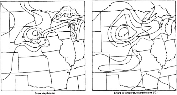
FIGURE 1
(a) Snow depth (cm) at 1200 UTC on 5 March 1977, and (b) 5-day average of the error (°C) of the daily maximum temperature forecasts for 5-9 March 1977 derived from the National Meteorological Center's Model Output Statistics. (From Dewey, 1977; reprinted with permission of the American Meteorological Society.)
cover. However, Lamb (1955) showed that there is a detectable decrease in the 1000 to 500 mb thickness as a layer of air passes over a large area of snow cover, implying that snow cover can contribute to the maintenance of a trough of cold air, which in turn helps to maintain the snow cover.
Some of the earliest work on the role of snow cover in seasonal atmospheric variability was directed at the Asian monsoon. Blanford (1884), Walker (1910), and others postulated a link between Himalayan winter snow cover and the strength of the Indian summer monsoon by reasoning that extensive snow cover could retard the heating of the Asian landmass. This link has been substantiated in recent years with the aid of satellite-derived measurements of snow cover (Hahn and Shukla, 1976; Dey et al., 1984; Dickson, 1984; Bhanu Kumar, 1988). On the basis of data for the 1967-1980 period, linear correlation coefficients between December-to-March snow extent in the Himalayas and June-to-September monsoon rainfall were found to be approximately -0.6 (Dey et al., 1984; Dickson, 1984).
While the monsoon-snow correlations seem to provide the basis for useful monsoon predictions at ranges of several months, there are several important caveats. First, snow cover over the Himalayan region was not mapped consistently during the first part (1967-1972) of the satellite record (Ropelewski et al., 1984). Second, as shown in Figure 2 (from Bhanu Kumar, 1987), the agreement between the interannual fluctuations of snowfall and monsoon variables has been noticeably poorer since 1980. Inclusion of data from 1981 to 1985 lowered the snow-rainfall correlations from -0.60 to -0.38 (r2˜0.14); the 95 percent significance threshold for a sample of N = 19 years is approximately 0.45. Third, Indian monsoon rainfall appears to correlate as highly with snow cover over the remainder of Eurasia as it does with Himalayan snow cover (Dickson, 1984). The physical linkage between snowfall and monsoon rainfall may therefore be more complicated than implied by the proposed effect of snow on the timing of the heating of the Himalayan and Tibetan region. For this reason, the modeling studies (e.g., Barnett et al., 1989) described below provide potentially important diagnostic information.
Other observationally derived linkages between snow cover and the atmospheric circulation over seasonal time scales have been addressed by Afanas'eva et al. (1979), who examined the position of the Planetary Upper-air Frontal Zone (PUFZ) over Eurasia during the autumn and spring. Time variations of the PUFZ and the snow boundary correspond closely (r = 0.78). However, as noted above, such correlations are at least partially attributable to the fact that the position of major upper-air features (e.g., the jet stream) is a primary determinant of the position of the snow boundary. Interannual variations of snow cover over Eurasia were also examined by Toomig (1981), who found that the annual value of the absorption of solar radiation at Soviet stations is a strong function of the springtime absorption, which in turn depends on the albedo during spring. Toomig also reported modest correlations (r ˜ 0.45) between the surface albedo of early spring and the surface air temperatures through July at several stations. A similar lag relationship
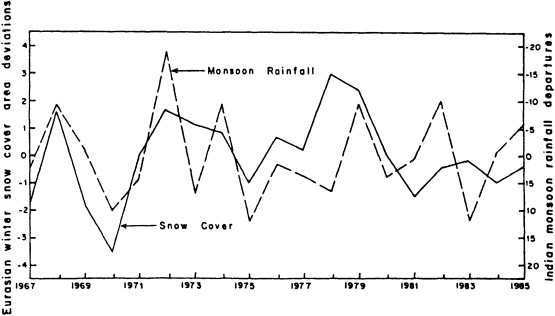
FIGURE 2
Variations of Eurasian winter snow cover and the corresponding summer monsoon rainfall over India. (From Bhanu Kumar, 1988; reprinted with permission of the Journal of the Meteorological Society of Japan.)
was suggested by Lamb (1972), who argued that the exceptionally cold summer of 1968 in northeastern Europe and northwestern Asia was attributable in part to the previous winter's extensive snow cover. Because the snow did not retreat until June and July, the ground remained cold and wet, thereby favoring the persistence of a trough. The attendant cloudiness and frequent cyclones produced above-normal rain and occasional snowfall throughout the summer over the northern Soviet Union. Wahl (1968) suggested that persistent snow may have played a similar role in the unusually cold summers of the 1830s in northern North America.
Feedbacks involving snow cover have been suggested by Namias (1962, 1981), who has argued that extensive snow cover over eastern North America should enhance the coastal baroclinicity and favor strong cyclones along the East Coast. These systems, in turn, reinforce the cold trough and contribute to its persistence over periods of several weeks or longer, as in the winters of 1960-1961 and 1976-1977. Dickson and Namias (1976) have attempted to link extensive snow/extreme cold over eastern North America with anomalies in the winter climatic regime of Greenland and northwestern Europe. According to the authors' hypothesis, the southward displacement and intensification of cyclones on the East Coast of the United States lead to a reduction of cyclone activity over the Iceland-Greenland region. This weakening of the Icelandic low reduces the advection of mild air into the northeastern North Atlantic and northern Europe, thereby increasing the frequency of polar outbreaks over the European land areas. The frequent recurrence of this abnormal winter regime during the 1960s may have contributed to the relatively extensive European snow cover during that decade. However, the role of snow cover in modifying the atmospheric circulation in such regimes remains speculative because other hypotheses (involving sea surface temperature anomalies, tropical forcing, etc.) can be formulated. Controlled model experiments are needed to explore the physical basis of seasonal anomalies in these specific cases, as has been done for anomalies such as the North American drought of 1988 and the ENSO event of 1982-1983 (e.g., Trenberth and Branstator, 1992; Palmer and Mansfield, 1986).
Iwasaki (1991) has recently reported a tendency for large-scale anomalies of snow cover to persist from December through February, but he found no indication of anomaly persistence from February to March in the longer data record. Iwasaki also reported an apparent lag relationship, in which winters with extensive snow cover over eastern Eurasia tend to be followed by winters with extensive snow cover over North America. Although this lag relationship is statistically significant (r = 0.52), at least three counterexamples occurred during the 1980s.
Modeling Studies
As the preceding subsection indicates, various roles have been attributed to snow cover in the evolution and persistence of monthly and seasonal atmospheric anomalies. Most of these roles involve feedbacks, which are notoriously difficult to unravel from observational data. Consequently,
model experiments provide a potentially useful vehicle for diagnosing the effects of snow cover. However, the mixed nature of the model-derived conclusions pertaining to the impacts of snow cover will become apparent as the survey proceeds.
In a study of snow-induced effects in non-winter months, Yeh et al. (1983) used a simplified version of the Geophysical Fluid Dynamics Laboratory's general-circulation model (GCM), containing idealized geography and a limited computational domain. The model contained no diurnal cycle, and its cloudiness was prescribed to be zonally uniform and seasonally invariant. The complete removal of the snow cover in mid-March was found to reduce the water available to the soil through snow melt, thus decreasing the soil moisture during the spring and summer in the region of snow removal. The drying of the soil resulted in an increase of surface temperature at high latitudes by 2°C to 8°C for the subsequent 3 to 4 months. The temperature increase extended into the upper troposphere, thereby reducing the meridional temperature gradient and the zonal wind in high latitudes.
A similar conclusion about the snow-hydrology-temperature linkage was obtained from a more realistic GCM by Yasunari et al. (1989). In this experiment, the 5° × 4° version of the Japanese Meteorological Institute GCM was run for 6 months beginning March 1. The experimental runs were identical to the control runs except for the addition of 5 cm (water equivalent) of snow in the snow-covered portion of the 30° to 60°N zone of the Eurasian continent. The results, shown in Figure 3, contained evidence of both (1) an albedo feedback, which suppressed temperatures over lower latitudes (e.g., Tibetan Plateau) by 2°C to 3°C during spring, and (2) a snow-hydrology-temperature linkage, which suppressed temperatures over middle latitudes by 2°C to 3°C during the summer months of June to August. During the summer, the anomalous Eurasian heat sink also appeared to induce a stationary Rossby wave
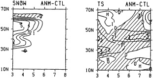
FIGURE 3
Latitude-time (month) sections of anomalies ("Heavy Snow" run minus "Control" run) of snow mass (cm liquid equivalent) and surface air temperature (°C) averaged over the Eurasian continent. (From Yasunari et al., 1989; reprinted with permission of the World Meteorological Organization.)
pattern extending from eastern Asia to northern North America.
The most thorough investigation of spring-summer feedbacks involving snow cover is Barnett et al.'s 1989 study of Eurasian snow impacts on a low-resolution (T2 1) version of the European Centre for Medium-Range Weather Forecasting's model. In Barnett et al.'s first experiment, snow extent corresponding to observed extremes was prescribed and interactions between snow and the surface hydrology were suppressed in order to isolate the albedo effect. The atmospheric response to the snow anomalies was local and confined primarily to air temperature and upper-air geopotential (but not sea-level pressure). All significant signals vanished when the snow disappeared in the spring, and the albedo effect had no sustained impact on the development of the Asian monsoon.
In Barnett et al.'s second experiment, rates of snowfall over Eurasia were doubled and halved so that the subsequent melt and evaporation could induce changes in the regional hydrology. The two sets of simulations showed statistically significant differences extending through the subsequent two seasons. The results derived from the doubled snowfall were characterized by significantly lower surface and tropospheric temperatures from May through July, higher pressures over Asia and lower pressures over North America, weaker zonal winds over the Arabian Sea, weaker surface convergence over southern Asia, and a weaker monsoon over southeast Asia. The Indian monsoon, however, was not substantially weaker in the "heavy snow" simulations, although this result may be partially attributable to the model resolution. The sea-level pressure signal over Asia and North America is stronger in the model than in the real world; the exchange of mass between the two continents may have been exaggerated in the model because the sea surface temperature (SST) distribution was prescribed climatologically in all the model runs.
In general, the physical mechanisms underlying Barnett et al.'s model response are similar to those of Yeh et al. (1983). The doubling of snowfall by Barnett et al. also produced a general weakening of the wind in the Southern Hemisphere and along the equator. While this response is similar to that which occurs prior to the warm phase of an ENSO event, the model with prescribed SST cannot sustain an ENSO event. In order to address the snow-ENSO link in more detail, Barnett et al. performed additional experiments with a coupled ocean-atmosphere model. The conclusion was that "the snow/monsoon signal has all the characteristics necessary to trigger the Pacific portion of an ENSO event, but the signal is too small by a factor of at least 2. In balance, it appears that snow-induced monsoon perturbations may be one of the (multiple) triggers that can initiate an ENSO cycle" (Barnett et al., 1989, p. 683-684). The elimination of major model biases and the improvement
of the model resolution are clearly high priorities in the context of this large-scale signal involving snow cover.
The studies summarized above suggest that snow cover may play a major climatic role regionally and perhaps even globally. However, the most recently published investigation of snow-climate interactions provides some indications of a negative feedback involving snow and temperature anomalies, at least during late winter and early spring. Cohen and Rind (1991) used the Goddard Institute for Space Studies 9-layer model with 8° × 10° resolution to examine the sensitivities to snow cover during March. The initial (March 1) boundary conditions corresponded to the observationally derived "maximum" and "minimum" snow cover and depth over North America and Eurasia. A key feature of this experiment was that the snow cover was interactive rather than prescribed. In the results of a five-case sample of March simulations, the positive snow anomalies caused only a short-term local decrease in surface temperature. There was no non-local signal, and even the local signal became weak after about 7 days. In the model physics, the reduction in the surface absorption of solar radiation and the increased consumption of latent heat for melting the snow contributed to lower temperatures. However, the remaining terms in the surface energy budget (e.g., long-wave radiation, sensible heat flux) adjusted so that they offset the cooling. Thus a negative feedback limited the impact of the snow anomalies to a slight cooling of about 1°C—a smaller effect than indicated by the observational studies and by the model experiment of Yasunari et al. (1989). This negative feedback that limits the albedo effect of snow was also found in Barnett et al.'s (1989) first experiment, and the weak signal is not inconsistent with the results of Robock and Tauss (1986), who used a simple, linear, steady-state model. Thus the relatively negligible impact of snow cover in the Cohen and Rind experiment may be due to the fact that their simulations did not extend into the spring season, when the hydrologic role of snow anomalies can become more important. The compatibility of the results from these various model experiments, nevertheless, requires further attention.
SNOW COVER AND ATMOSPHERIC VARIABILITY: DECADE-TO-CENTURY TIME SCALES
The importance of snow cover for climate change over decade-to-century time scales depends on several factors. First, changes in other components of the climate system are likely to alter the large-scale distribution of snow cover. Relatively small shifts in the atmospheric circulation pattern can have major effects on the snow distribution in mountainous areas, e.g., the Rocky Mountains (Changnon et al., 1993). The extent to which snow cover will change in response to a changing climate is not well known; for example, a general warming may increase snow melt and decrease the fraction of precipitation that falls as snow, but (according to models) it is likely to increase precipitation in high latitudes-where most precipitation falls as snow. In view of these competing effects, it is conceivable that snow extent could decrease while high-latitude snow volume increases. Second, changes of snow cover can trigger a host of potential feedbacks involving air temperature, soil moisture, cloudiness, the phasing of the seasonal cycle, and other variables. The magnitudes and relative importance of these feedbacks are poorly known. The individual feedbacks are notoriously difficult to isolate in observational data. Although various model experiments have addressed individual feedbacks, the isolation of individual feedbacks can be a nontrivial undertaking even in model simulations.
In the section below, we address the first of the two factors listed above by surveying recent analyses of observational data pertaining to snow cover. We then address the issue of snow-related feedbacks in climate change by surveying the recent model experiments that may be most relevant to changes over the decade-to-century time scales.
Observational Studies
Observational studies of historical variations of snowfall, snow depth, and snow water equivalent are confounded by measurement difficulties pertaining to small-scale variations of these variables. Large spatial gradients of all three variables are found over areas containing even moderate topographic features. Moreover, snow gauges are known to "undercatch" snow; the degree of undercatch varies with the type of gauge, and the type of gauge has changed during the period of record at nearly all stations. While satellite data have provided essentially continuous global coverage since the early 1970s, the useful information is generally limited to areal extent. The critically needed mapping of snow depth or water equivalent is not yet achievable over large areas, although algorithms for snow depth in vegetation-sparse areas have been used with some success (Chang et al., 1987).
The most comprehensive analysis of satellite-derived data on snow coverage was made by Robinson and Dewey (1990), who found that the Northern Hemisphere snow cover of recent years is less extensive than that of 10 to 20 years ago. Perhaps coincidentally, the increase of surface temperature over the last few decades is larger over land than over the oceans. The high-latitude land areas, which are generally snow covered during winter, show the strongest warming (Figure 4; see color well); this warming has been strongest in spring and winter. In a recent analysis of North American data, Karl et al. (1993) identified several regions that, because of their high variability of snow cover, have exerted the primary influence on North American snow variations. These regions, which vary seasonally, are ones in which the inverse snow-temperature relationship is
strong. Karl et al. also used station data to extend their analysis to the multidecade-to-century time scale. Their findings included a 4 to 5 percent increase of both solid and total precipitation rates over northern Canada during the past four decades, century-scale increases of precipitation over southern Canada and the contiguous United States, and a decrease in the proportion of precipitation falling as snow in southern Canada. These findings are generally consistent with the changes that have been hypothesized to accompany a greenhouse warming. Karl et al. also found that the unprecedented warmth of the 1980s in Alaska was accompanied by a 10 percent increase of annual precipitation in that region. Leathers and Robinson (1993) have examined the winter region (the central United States) in more detail, finding that the concurrent 500 mb height anomalies are generally collocated with the snow/temperature anomalies during December but not during January and February.
The general coincidence of the "marginal snow zone" and the areas of strongest warming over the past several decades (Figure 4) deserves further comment with regard to the possible nature of the forcing. The "land-leading-ocean" feature is characteristic of large-scale forcing such as global warming or the response to major volcanic events. By contrast, natural low-frequency variations will generally manifest themselves in an "ocean-leading-land" pattern because the ocean is the low-frequency source of the forcing on the near-surface atmospheric temperature. The extent to which a large-scale forced temperature response is amplified by the retreat of snow over land is one of the key unknowns in the interpretation of a pattern such as that in Figure 4.
Decadal-scale summaries of snowfall in China have been compiled by Li (1987), who found a decrease of snowfall over China during the 1950s followed by an increase during the 1960s and 1970s; the late 1970s had the largest running-mean values of the 30-year period of record (Figure 5). Li noted a general correspondence between the time series of global mean temperature and mean snow depth in China (as well as an apparent association between years of heavy
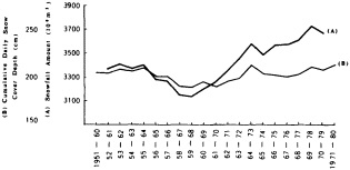
FIGURE 5
Ten-year running mean of horizontally integrated snow depth and amount in China. (From Li, 1987; reprinted with permission of IAHS Press.)
snow and ENSO events). Similar compilations have been made for other regions such as the Swiss Alps (Lang and Rohrer, 1987), although the representativeness of such time series is a key issue. From the standpoint of areal coverage, the snowfall records that are potentially most valuable are those of the former Soviet Union. The status of these data is uncertain.
The longest time series of snow cover are generally those coming from single stations (e.g., the Tokyo record dating back to the 1630s (Lamb, 1977)) or the records of annual precipitation derived from polar ice cores (e.g., the Greenland Ice Sheet Project's work in Antarctica and Greenland, as in Alley et al., 1993). The cores represent potentially valuable records of regional snowfall if the spatial representativeness of the point data can be established. The South Pole data, for example, have been used to deduce an increase of snowfall from the 1700s to the early twentieth century (Giovinetto and Schwertfeger, 1966; Lamb, 1977). Analysis of GISP's Greenland cores has only recently begun (Mayewski et al., 1993).
Another type of data for which analyses are in the early phases is the runoff (stream-flow) data for the high-latitude rivers that are fed primarily by snow melt. Mysak et al. (1990) have proposed a mechanism by which an interdecadal (approximately 20-year) cycle results from a feedback loop involving high-latitude precipitation, runoff, arctic sea-ice export to the North Atlantic, and ocean salinity/temperature anomalies. The linkages involving snowfall and runoff have yet to be thoroughly evaluated. In view of the potential implications of this cycle for the global ocean circulation, quantitative analyses of high-latitude snowfall and runoff are being assigned high priority in the upcoming ACSYS (Arctic Climate System) component of the World Climate Research Program. The extension of such analyses to include soil moisture and land surface temperatures also appears to merit high priority in the context of possible greenhouse-induced changes over decadal time scales.
Finally, glaciers are ultimately attributable to continental snowfall over time scales of decades to millennia. The advance and retreat of glaciers have long been regarded as proxy indicators of climate change over these time scales. In the context of global change, the key properties of glaciers are extent, ice volume, and mass balance. Temporal changes in these glacial properties can be complex functions of temperature, precipitation, the seasonality of temperature and precipitation, and topography. Nevertheless, the advance and retreat of glaciers are known to be consistent with century-scale changes of regional climate, e.g., the Little Ice Age.
Field measurements of glaciers are now assembled and reported by the World Glacier Monitoring Service in Zürich. These data, which are summarized by Haberli et al. (1989), include direct measurements of the mass balance of approximately 75 glaciers in the Northern Hemisphere. Statistics on
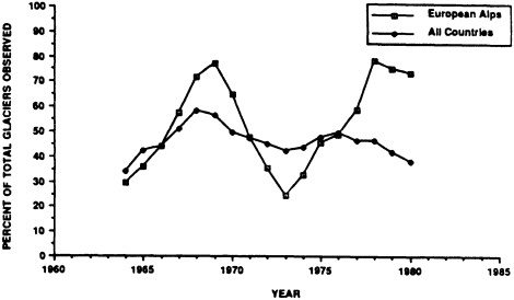
FIGURE 6
Five-year moving averages of percentage of glaciers having positive mass balance. (From Wood, 1988; reprinted with permission of the University of Colorado.)
glacial changes have been compiled for about 500 glaciers worldwide (e.g., Wood, 1988). Figure 6 (from Wood, 1988) shows the trends in glacier mass balance over approximately 20 years, expressed as the percentage of observed glaciers having a positive mass balance. While this percentage for all glaciers is close to 50 percent, the percentage for an individual region such as the European Alps can undergo multi-year excursions well above or below 50 percent.
Modeling Studies
Aside from CO2-doubling experiments, there have been very few three-dimensional model simulations of the land-atmosphere system over decadal time scales. In this respect, one may argue that less attention has been given to the simulation of land-atmosphere interactions than to the simulation of large-scale ocean variations over decade-to-century time scales. Examples of the latter are the experiments of Bryan (1986), Weaver et al. (1991), and Yang and Neelin (1993). Moreover, most models containing an interactive land surface treat the surface physics quite crudely: the "bucket" method is typically used to handle soil moisture, multi-level soil treatments are generally not included, and runoff often "disappears" from the system.
Most global climate models do include a thermodynamically and hydrologically interactive snow cover. In its assessment of climate models, the IPCC (1990) found that the snow cover simulated by several models was "broadly realistic," leading to the statement that "the simulated snow extent should thus not distort the simulated global radiative feedbacks" (IPCC, 1990, p. 113). Even if one gives the benefit of the doubt to that assertion, the snow cover simulated by all models appears to contain significant errors, particularly over eastern Asia. More comprehensive diagnostic assessments of the simulated snow cover (extent and water equivalent) in the context of both the present climate and projections of climate change are needed.
A more sobering finding concerning model simulations of the feedback between snow and radiation is contained in the IPCC's (1992) update, which cites Cess et al.'s (1991) comparison of the snow feedback (under perpetual April forcing) in 17 global climate models. The temperature sensitivity or feedback parameter, λ, associated with snow cover was found to vary from negative values in some models to a wide range of positive values (Figure 7). The sensitivity parameter in clear-sky regions ranges from values corres-
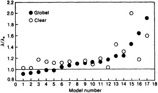
FIGURE 7
Snow feedback parameter for 17 general-circulation models. Solid circles denote global values, open circles denote values for clear-sky regions. (From Cess et al., 1991; reprinted with permission of the American Association for the Advancement of Science.)
ponding to negligible snow feedback to values representing a twofold amplification. Cloudiness complicates the interpretation of the snow feedback even further. The IPCC concludes that "the snow-albedo-temperature feedback processes in models are somewhat more complex" (IPCC, 1992, p. 117) than the conventional interpretation of the positive snow-albedo-temperature enhancement of a perturbation. Since these models also generally lack realistic surface hydrologies, one must view with caution their simulations and/or projections of atmosphere-snow interactions.
The model experiments of Yeh et al. (1983), Barnett et al. (1989), Yasunari et al. (1989), and Cohen and Rind (1991), all of which were summarized above, are potentially relevant to decade-to-century-scale climatic change even though the simulation periods are subdecadal. This relevance stems from the fact that climate changes over decadal time scales may perturb the large-scale snow distribution by amounts comparable to the changes of snow prescribed in the modeling experiments. However, biases introduced by the parameterizations of the snow and surface physics must be addressed before the results of the experiments can be viewed with confidence. A step in this direction has been made by Washington and Meehl (1986), who found that the inclusion of a simple temperature dependence in the parameterization of snow albedo can change substantially the globally averaged surface temperature increase caused by a doubling of CO2. Ingram et al. (1989) and Covey et al. (1991) also examined the effects of high-latitude surface albedo parameterizations, although their experiments focused on sea-ice-albedo. Using an earlier generation of the National Center for Atmospheric Research's model, Williams (1975) found that changes in surface albedo (and SST) influenced a simulated ice-age circulation more than did the orographic changes caused by the glaciation. Further surface-sensitivity experiments with more current atmospheric models and with more realistic treatments of the surface physics and hydrology are needed.
An issue in need of particular attention is the apparent paradox involving recent observational data (on snow and air temperature) and modeling studies of the feedback between snow, soil moisture, and temperature. The modeling studies cited above indicate that a positive anomaly of snow cover tends to depress surface air temperatures through its enhancement of soil moisture for up to several months after the snow melt. The model results seem inconsistent with the observed tendencies toward higher springtime temperatures and increases of snowfall in northern land areas over the past several decades. However, an earlier retreat of snow during the late winter or early spring may be a consequence of the warming, which is most pronounced in the winter and spring seasons, especially if the increases of snow depth have occurred primarily in the northernmost land areas (as the data suggest they have). The earlier retreat of snow creates the possibility that the albedo effect may offset, or even dominate, the tendency of greater soil moisture to delay the seasonal warming. Since this scenario is especially likely if the upper layers of soil dry rapidly, it is clearly important that models accurately resolve the hydrological and thermal changes in the upper layers of the land surface during the snow-melt period. The potentially high climatic leverage of the snow-melt period should make it a focus of observational and modeling studies, whether the time scales of interest are decadal or century or even longer.
CONCLUSION
Several conclusions emerge from the results surveyed here. The first, which pertains to the strategy for diagnosing the role of snow cover in climate variability, is that both modeling and data analysis are essential and complementary diagnostic tools. Because snow is involved in a variety of interactions within the climate system, and because the distribution of snow is determined largely by other components of the climate system, controlled experimentation with numerical models is a key element of the diagnostic strategy. However, the biases and other limitations of models are such that numerical experiments yield convincing conclusions only when the observational data give some credibility to the model results.
The diagnostic studies of the past few decades appear, at first glance, to have produced a somewhat inconclusive picture of the climatic role of snow cover. However, several scientific conclusions do emerge when the results are viewed in an aggregate sense:
-
Anomalies of snow cover are clearly associated with significant local anomalies of air temperature, at least in the lowest 100 to 200 mb. The duration of these local anomalies generally ranges from several days to several weeks and is often limited by the fluctuations of the snow anomalies themselves over weekly and monthly time scales.
-
Over the past two to three decades, changes of surface air temperature are broadly consistent with changes of snow coverage, especially in winter and spring.
-
There is little or no evidence that the albedo effect of wintertime snow anomalies produces meaningful signals in the large-scale atmospheric circulation.
-
The snow-hydrology-soil moisture feedback appears to be capable of producing a meaningful response in the atmosphere during spring and summer. The scale of this response is at least regional and possibly larger. Regions susceptible to snow-hydrology effects include eastern Asia and the northern portions of Eurasia and North America.
-
The mechanism(s) by which snow influences the large-scale atmosphere are sufficiently complex that rela-
-
tively sophisticated (e.g., nonlinear) models are required for the diagnosis of snow-atmosphere interactions.
With regard to (4) and (5), the validity of parameterizations involving snow cover in global climate models may be a major constraint on further progress toward an understanding of snow-atmosphere feedbacks. Priority should be given to the parameterization of quantities and processes such as snow surface albedo, the influence of snow on the boundary layer structure, and the disposition of the liquid water produced by snow melt.
ACKNOWLEDGMENTS
The preparation of this paper was supported by the National Science Foundation through Grants DPP-9214793 and ATM-9319952. We thank Norene McGhiey for typing the manuscript.
Commentary on the Paper of Walsh
DAVID A. ROBINSON
Rutgers University
Rather than commenting on Dr. Walsh's paper, I am going to show you a little about my work on hemispheric snow cover over the last several decades and also on the century time scale I am beginning to put together. This is at Dr. Walsh's suggestion, I hasten to add.
Figure 1 gives you an idea of the annual cycle of snow cover over Northern Hemisphere lands. The area covered by snow ranges from 40 to 50 million km2 during the winter over the Eurasian and North American continents to several million km2 in summer, primarily on top of the Greenland ice sheet.
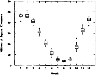
FIGURE 1
Monthly snow cover over Northern Hemisphere lands (including Greenland) between January 1972 and August 1991. The median area of cover is the horizontal line within the 12 monthly boxes, and the interquartile range (ICR) is between the top and bottom of the box. Whiskers show the extreme values between + 1 and + 1.5 times ICR and between - 1 and - 1.5 times ICR, and asterisks show values outside these ranges. Values are calculated from NOAA weekly snow charts.
In recent years there has been a dearth of snow cover over Northern Hemisphere lands (cf. Figure 3 in my paper in this volume). It has been true for the last 5 to 6 years over both Eurasia and North America. So it is seen hemisphere-wide, with many record lows set in the last couple of years, particularly 1990. I remind you that this is based on 20 years of observation. Nonetheless, this record, produced weekly by NOAA, happens to be the most consistent long-term satellite-derived data set available for any climatic variable. Charts go back to 1966, but most of us who have looked at the data feel that it is relatively homogeneous and credible only from 1972 on.
Looking at seasonal variations in snow cover over the past 20 years (cf. my Figure 4 in this volume), you see that there has been very little variation over the winter seasons in Eurasia, and even less in North America. This agrees with what Dr. Walsh showed earlier for sea ice. Fall cover has varied a bit more, but spring and summer show the greatest year-to-year variations in cover. In recent years snow cover has decreased in March through June over both North America and Eurasia. These spring decreases in recent years have been most pronounced over northeastern Asia and down the leeward side of the Canadian Rockies into the northern portions of the United States.
So that is what we have seen hemispherically over the past 20 years. Unfortunately, we have no data sets going back longer than that on a hemispheric scale, but there have been some recent efforts to try to extend local and regional data sets back to the turn of the century. For instance, at Denison, Iowa, over the course of this century there appears to be an increase in the number of snow-covered days with =1 inch (2.5 cm) of snow on the ground during the fall, winter, and spring.
As for other data sets to examine, we are beginning to sort out daily data from a set containing several hundred Russian stations. In some cases, the records go back to the turn of the century. We have also been examining station data in western China extending back into the 1950s.
Discussion
NORTH: The warming pattern John mentioned, with the leading in the middle of the continental areas and the lagging in the ocean, seems to be a very robust feature. It seems to hold for transient runs for all models, and even toy models have it. I think it's something that needs to be put into the filter when you're trying to do the signal processing I mentioned earlier. You get an increase on the order of 30 percent in the signal-to-noise ratio.
This same land-leading-ocean feature will appear when you have a large-scale forcing. But when it's natural variability at very low frequencies, the ocean tends to lead—for example, with Mt. Pinatubo. It would be interesting to look at the phase relations during the 1940s, when the cooling was so dramatic in the Northern Hemisphere, to see whether the sea ice was leading.
DELWORTH: In the GFDL model for natural variability, for time scales less than 50 years, the continental-region temperatures actually correlate most with the hemispheric means. It's complex, but I think you have to go to longer time scales to get the deep ocean involved.
SHUKLA: I wonder about the apparent paradox of a higher snow amount's being succeeded by warming and reduction in area in the following season.
WALSH: If the snow is disappearing earlier because of the greater springtime warmth, the perturbation of soil moisture due to the extra snow may just be swamped. The additional solar radiation available may be a larger effect than the soil moisture. Also, we don't know that the time scales of the soil perturbations in the model agree with the real world's.
ROBINSON: You might also have different effects deep within the pack and near the periphery.
RASMUSSON: One of the contributors to the recent warming over Eurasia was the exceptionally warm winter of 1982-1983. We were mystified by it, since it was not supposed to be associated with the 1982-1983 El Niño event, but Alan Robock's work on volcanic eruptions suggests that it could have been a response to El Chichon. Also, Dave, I wondered whether you had been able to clear up the snow-cover data problems you were having.
ROBINSON: Yes; I found that two different land masks had been used in the 1970s and 1980s, both of which were wrong. Using GIS techniques, I've come up with a land mask and a procedure that yield consistent and reasonably accurate numbers.
RIND: One caveat: The model run you looked at did not have one additional forcing, the reduction in ozone in the lower stratosphere. That is most effective at polar regions, and would also induce a cooling trend at the surface.
BRYAN: It seems to me that the resemblance to a greenhouse effect that appeared in the slide you showed for the 30-year average may be at least partly an artifact of the averaging—a combination of a very cold event at the beginning of the period and warming over land masses toward the end. I think it could be a little misleading to compare it with the slow warming observed in the greenhouse model experiment.
WALSH: I agree with your comment on the land, but the changes were actually negative over the high-latitude oceans during that period, so I don't think the start can have been unrepresentative.
NORTH: The Hanson-Lebedeff paper of 1988 or so, which was for a longer period leading up to the 1940s, showed the same kind of pattern.
TRENBERTH: I feel obliged to mention that the Southern Hemisphere has snow cover and sea ice too. I know Claire Parkinson has done some work there; can you comment, John?
WALSH: There's essentially no snow there outside the Antarctic continent. The one thing we know from the 20-year satellite record of the South Orkneys is that those data are not representative of the larger-scale changes.
ROBINSON: Ken Dewey and Randy Cerveny are doing a little work with snow over Patagonia and other areas.
JONES: Returning to an earlier point, I wanted to say that the temperature variations at the two Antarctic inland stations and Vostok over the past 35 years are similar to what we've seen around the coast. Since Greenland is a much smaller ice sheet than Antarctica, we may be able to infer that the temperature changes in its interior would also be similar to those measured around the coast.
KUSHNIR: Just a correction to an earlier suggestion: The coldest temperatures in the Atlantic were in the 1970s, not the 1960s, so John may indeed be picking up a trend.
GROISMAN: I'd like to note that it's important that John found the changes in sea ice in summer. Wintertime ice can go back to its old limits, but the new ice is most easily melted off in the spring.
Decadal Variations of Snow Cover
DAVID A. ROBINSON1
ABSTRACT
In situ and satellite observations of snow-cover duration show a considerable amount of year-to-year variability on local to hemispheric scales. This variability is often embedded in longer-term fluctuations. In situ data from the central United States indicate multi-decadal fluctuations in the duration of snow over the past century, and hemispheric satellite observations suggest variations lasting for several years or more.
Such analyses have become possible in recent years as a result of the recovery, digitization, and validation of historic in situ observations of snow cover and the availability of two decades of satellite observations of continental snow cover. Efforts are needed to recover additional historic data, to improve the recognition of snow using microwave satellite data, and to create global snow products using all available data sources. With these data available for analysis, knowledge of the spatial and temporal kinematics of snow cover will continue to improve. This will contribute to a better understanding of the role of snow in the climate system and to the utility of snow as an indicator of climate change.
INTRODUCTION
Snow cover is a critical influence on the earth's climatic energy and hydrologic budgets. In many regions it may play an influential role in determining the magnitude of any human-induced climate change, and might be a useful indicator and monitor of such change. To understand better the importance of snow in the climate system, it is essential that accurate information on the temporal and spatial dimensions of snow cover be available. Such data have been obtained through in situ and satellite observations, and recent efforts have begun to locate, assimilate, and validate these data. Once available, they are being employed in empirical and modeling investigations of snow-cover kinematics and the dynamical aspects of snow within the climate system. An excellent survey of the latter is provided by Walsh (1995) earlier in this section. This paper will concentrate on the distribution of snow cover in space and time over the past two decades and the past century. Much of the discussion will focus on the newly available in situ and satellite data sets. Given the lack of attention paid to secular snow cover data until recently, only limited analyses of these data have taken place. A few examples of these efforts
will be presented. For information on snowfall and its long-term variability across the North American continent, the paper later in this section by Groisman and Easterling (1995) is recommended.
IN SITU OBSERVATIONS
In situ snow-cover data are gathered mainly over land. Only a few short-term studies have measured snow on sea ice or ice sheets (e.g., Hanson, 1980). Most observations on land are made on a once-per-day basis. The general practice is to record the average depth of snow lying on level, open ground that has a natural surface cover. At primary stations, the water equivalent of the snowpack may also be measured. In some regions, snow courses have been established where snow depth, water equivalent, and perhaps other pack properties are measured along prescribed transects across the landscape. Observations are often made only once per month, and the number of courses is extremely limited in North America. More frequent and abundant course data are gathered in the Commonwealth of Independent States, and currently this information is being recovered through a cooperative effort between the U.S. National Snow and Ice Data Center (NSIDC) at the University of Colorado and A. Krenke of the Russian Academy of Sciences.
Current station observations of snow cover are of a sufficient density for climatological study in the lower elevations of the middle latitudes. Elsewhere, while data of a high quality are gathered at a number of locations (Barry, 1983), the spatial and temporal coverage of the information is often inadequate for climate study. There is no hemispheric snow-cover product based entirely on station reports. The U.S. Air Force global snow-depth product depends heavily on surface-based observations as input into a numerical model that creates daily charts with global coverage, but it must rely on extrapolations and climatology in data-sparse regions (Hall, 1986; Armstrong and Hardman, 1991). There have been a number of regional snow-cover products over the years that are based on station data. Of greatest longevity are the Weekly Weather and Crop Bulletin charts, which have been produced since 1935. These, and the daily NOAA charts, are produced for the conterminous United States mainly from first-order station observations. Therefore, neither has a particularly high resolution, and observations may be influenced by urban heat-island effects.
In a number of countries, there are numerous stations with relatively complete records of snow extending back 50 years or more (Barry and Armstrong, 1987). Until recently, most data have remained unverified and disorganized (Robinson, 1989). As a result, few studies have dealt with long-term trends or low-frequency fluctuations of snow over even small regions (e.g., Arakawa, 1957; Manley, 1969; Jackson, 1978; Pfister, 1985). Through the cooperative efforts of a number of scientists and data centers, this situation has begun to be rectified. Examples include the exchange of data through the US/USSR Bi-Lateral Environmental Data Exchange Agreement and between the Lanzhou Institute of Glaciology and Geocryology and both Rutgers University and the NSIDC. These and other data are in the process of being quality controlled, and routines to fill in gaps in snow-cover records are being developed (Hughes and Robinson, 1993; Robinson, 1993a). Clearly, there is a need to continue efforts to identify, assimilate, in some cases digitize, and in all cases validate station and snow-course observations from around the world. These data must also must be accompanied by accurate and complete metadata.
Lengthy in situ records continue to be analyzed for individual stations, and data from networks of stations have begun to be studied on a regional level. For example, marked year-to-year variability in snow-cover duration is recognized over the course of this century at Denison, Iowa (Figure 1). Snow at least 7.5 cm deep has covered the area for as much as 80 percent of the winter, but in a number of years no or only a few days have had a cover this deep. Overall, the duration of winter and spring cover was at a maximum in the 1970s, and fall cover peaked in the 1950s. Other periods of more frequent winter cover include the 1910s and the late 1930s to early 1940s. The 1920s, middle 1940s, and late 1950s to early 1960s were periods with less abundant winter cover. Missing data around 1950 prohibit a direct assessment of winter cover at Denison, but adjacent stations suggest cover was scarce at this time. All three seasons show a greater abundance of snow-cover days in the past 40 years than in the first half of the century.
Efforts are under way to develop gridded snow files for a large portion of the central United States, using data from several hundred stations. Raw and filtered winter records from four of these stations are shown in Figure 2. They are for days with snow cover =7.5 cm, and all indicate long-term fluctuations on the order of one to several decades. The Nebraska and Kansas stations show maximum durations during the past several decades, with a similar early maximum at Oshkosh, Nebraska, in the 1910s and early 1940s. Late 1920s, early 1950s, and 1970s maxima were observed at Dupree, South Dakota, the latter two ending abruptly shortly thereafter. The North Dakota station had maximum winter snow cover in the 1930s, around 1950, and in the late 1970s. The range in filtered values over the period of record was approximately two weeks in Kansas and Nebraska and seven weeks in South Dakota and North Dakota.
SATELLITE OBSERVATIONS
Snow extent is monitored using data recorded in short-wave (visible and near-infrared) and microwave wave-
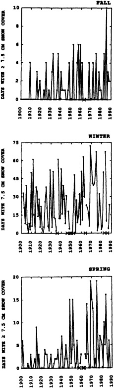
FIGURE 1
Time series of fall (September-November), winter (December-February), and spring (March-May) days with =7.5 cm of snow cover at Denison, Iowa. Missing years are marked with an X.
lengths by sensors on board geostationary and polar orbiting satellites. Retrieval techniques, the strengths and limitations of each spectral region for sensing snow, and the snow products derived using short-wave and microwave input are discussed in this section. The secular remote sensing of snow over Northern Hemisphere lands will be the principal focus; only a few efforts have addressed this over Southern Hemisphere lands (Dewey and Heim, 1983) or Arctic sea ice (Robinson et al., 1992).
Short-Wave and Microwave Snow Charting
Short-wave data provide continental coverage of snow extent at a relatively high spatial resolution. Snow is identified by recognizing characteristic textured surface features and brightness. Information on surface albedo and percentage of snow coverage (patchiness) is also gleaned from the data. Shortcomings include (1) the inability to detect snow cover when solar illumination is low or when skies are cloudy, (2) the underestimation of cover where dense forests mask the underlying snow, (3) difficulties in distinguishing snow from clouds in mountainous regions and in uniform, lightly vegetated areas that have a high surface brightness when covered with snow, and (4) the lack of all but the most general information on snow depth (Kukla and Robinson, 1979; Dewey and Heim, 1982).
Microwave radiation emitted by the earth's surface penetrates winter clouds, permitting an unobstructed signal from the surface to reach a satellite. The detection of snow cover from microwave data is possible mainly because of differences in emissivity between snow-covered and snow-free surfaces. Estimates of the spatial extent, as well as of the depth or water equivalent, of the snowpack are derived from equations that employ measurements of radiation sensed by multiple channels in the microwave portion of the spectrum (e.g., Kunzi et al., 1982; McFarland et al., 1987). Estimates of snow cover have been made using microwave data since the launch of the Scanning Multichannel Microwave Radiometer (SMMR) in late 1978. The spatial resolution of the data is approximately several tens of kilometers. Since 1987, close to the time of SMMR failure, the Special Sensor Microwave Imager (SSM/I) has provided data. Both sensors, having nearly the same spectral characteristics, have similar levels of success in monitoring snow extent (cf. the SMMR analyses below).
As with short-wave products, the microwave charting of snow extent is not without its limitations. The resolution of the data makes the detailed recognition of snow cover difficult, particularly where snow is patchy, and it is difficult to identify shallow or wet snow using microwaves. Also, the lack of sufficient ground-truth data on snow volume, wetness, and grain size makes an adequate assessment of the reliability of microwave estimates uncertain. The influence of a forest canopy on microwave emissions in snow-
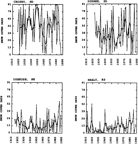
FIGURE 2
Time series of winter days with =7.5 cm of snow cover at four stations on the U.S. Great Plains. Also shown smoothed with a nine-point binomial filter, with only those points plotted where nine years are available for filtering (i.e., plotted year ±4 yr).
covered regions, which is currently not well understood, must also be taken into account when estimating snow cover. Because of the region-specific differences in land cover and snowpack properties, no single algorithm can adequately estimate snow cover across Northern Hemisphere lands.
Hemispheric Snow Products: NOAA Weekly Charts
In 1966, NOAA began to map snow cover over Northern Hemisphere lands on a weekly basis (Matson et al., 1986). That effort continues today, and remains the only such hemispheric product. NOAA charts are based on a visual interpretation of photographic copies of short-wave imagery by trained meteorologists. Up to 1972, the sub-point resolution of the meteorological satellites commonly used was around 4 km; since then it has become, and remained, close to 1.0 km. Charts show boundaries on the last day that the surface in a given region was seen. Since May 1982, dates when a region was last observed have been placed on the charts. An examination of these dates shows the charts to be most representative of the fifth day of the week.
It is recognized that in early years the snow extent was underestimated on the NOAA charts, especially during fall. Charting improved considerably in 1972 with the improvement of sensor resolution, and since then charting accuracy
has been such that this product is considered suitable for continental-scale climate studies (Kukla and Robinson, 1981). The NOAA charts are most reliable where skies are frequently clear, solar illumination is high, snow cover is reasonably stable or changes slowly, and pronounced local and regional signatures are present owing to the distribution of vegetation, lakes, and rivers.
The NOAA charts are digitized on a weekly basis using the National Meteorological Center Limited-Area Fine Mesh grid. This is an 89 ´ 89 cell Northern Hemisphere grid, with cell resolution ranging from 16,000 to 42,000 km2. If a cell is interpreted as being at least 50 percent snow covered, it is considered to be completely covered; otherwise it is considered to be snow free. Inconsistencies in the designation of a cell as land or water have occurred in the past during the digitization process. This has recently been resolved for the approximately 100 cells in question through the use of digital map files analyzed on a geographic information system (Robinson, 1993b).
A new routine for calculating monthly snow areas from the NOAA data has also recently been developed (Robinson, 1993b). This has eliminated previous inconsistencies resulting from undocumented changes in the methods used by NOAA to calculate the monthly values (Robinson et al., 1991). The new Rutgers Routine calculates weekly areas from the digitized snow files and weights them according to the number of days of a given week that fall in the given month. A chart week is considered to center on the fifth day of the published chart week (cf. above). No weighting has been employed in the NOAA routines.
Hemispheric Snow Products: NASA Microwave Files
Monthly charts of Northern Hemisphere continental snow extent have been produced from SMMR data by NASA scientists (Chang et al., 1990). The only such time series available to date, it covers the interval from November 1978 through August 1987. A single algorithm is used to estimate snow depth on a 0.5° × 0.5° grid. This theoretical algorithm uses the difference in brightness temperatures of 18 and 37 GHz SMMR data to derive a snow-depth/brightness temperature relationship for a uniform snow field. A snow density of 0.3 g/cm3 and a snow-crystal radius of 0.3 mm are assumed; fitting the differences to the linear portion of the 18 and 37 GHz responses permits the derivation of a constant that is applied to the measured differences. This algorithm can be used for snow up to 1 m deep.
The monthly depth estimate for a given grid cell is calculated by averaging depths reported for the five or six pentad charts centered in a given month (SMMR data are gathered every other day and three of these passes are used for each pentad chart; there is a one-day gap between each pentad). If the average is =2.5 cm, the cell is considered to be covered with snow for the whole month. This methodology biases the snow areas to the high side, especially in those areas and periods where snow cover fluctuates.
Northern Hemisphere Continental Snow Cover: 1972-1992
According to the NOAA snow charts, the extent of snow cover over Northern Hemisphere lands varies from 46.5 million km2 in January to 3.9 million km2 in August (Table 1); most of August's snow lies on top of the Greenland ice sheet. The past two decades of monthly data are close to normally distributed, and monthly standard deviations range from 0.9 million km2 in August to 2.9 million km2 in October. The annual mean cover is 25.5 million km2 with a standard deviation of 1.1 million km2. The snowiest year was 1978, which had a mean of 27.4 million km2; 1990 was the least snowy at 23.2 million km2. Eight of the monthly minima for the two decades occurred in 1990.
With only two decades of reliable hemispheric information, it is impossible to identify anything in the way of trends or cycles in the temporal or spatial distribution of snow. What has become recognizable during the period of record is a tendency for multi-year departures in snow cover, in which less pronounced month-to-month and season-to-season departures are embedded. Twelve-month running means illustrate the periods of above-normal cover that occurred in the late 1970s and mid-1980s, and the lower and below-normal extents during the mid-1970s and early 1980s (Figure 3). The most significant lengthy departure during the past 20 years began in the late 1980s and continued into 1992. Of the 65 months between August 1987 and December 1992, only eight had above-normal snow cover. Three of these eight were September, November, and December 1992.
Spring cover has shown pronounced deficits over the past five years in Eurasia and six years in North America; areas in these springs have been at or below lows established before this period (Figure 4). During the same interval, both continents have had low seasonal cover in the fall and summer, although frequently neither continent has been at or approached record low levels. Winter cover has been close to average over the past six years.
The NOAA snow estimates are considered the most accurate figures available. Despite the positive methodologically induced bias of the monthly NASA estimates (cf. the previous section), they range from less than I million up to 13 million km2 below the NOAA area estimates for those nine years for which both agencies provide estimates. These absolute differences are greatest in the late fall and early winter. In a relative sense, microwave areas are between 80 and 90 percent of short-wave values in winter and spring, 20 to 40 percent of the short-wave estimates in summer, and 40 to 70 percent of short-wave areas in fall. Possible explanations for the significant disparities in the latter two seasons are wet and shallow snows. These are difficult if
TABLE 1 Monthly and Annual Snow Cover (million km2) over Northern Hemisphere Lands, Including Greenland
|
|
Maximum (yr) |
Minimum (yr) |
Mean* |
Median |
Standard Deviation |
|
|
Jan |
49.8 (1985) |
41.7 (1981) |
46.5 |
46.1 |
1.8 |
|
|
Feb |
51.0 (1978) |
43.2 (1990,92) |
46.0 |
45.6 |
2.0 |
|
|
Mar |
44.1 (1985) |
37.0 (1990) |
41.0 |
40.8 |
1.9 |
|
|
Apr |
35.3 (1979) |
28.2 (1990) |
31.3 |
31.4 |
1.8 |
|
|
May |
24.1 (1974) |
17.4 (1990) |
20.8 |
20.6 |
1.9 |
|
|
Jun |
15.6 (1978) |
7.3 (1990) |
11.6 |
11.4 |
2.1 |
|
|
Jul |
8.0 (1978) |
3.4 (1990) |
5.3 |
5.5 |
1.2 |
|
|
Aug |
5.7 (1978) |
2.6 (1988,89,90) |
3.9 |
3.8 |
0.9 |
|
|
Sep |
7.9 (1972) |
3.9 (1990) |
5.6 |
5.6 |
1.1 |
|
|
Oct |
26.1 (1976) |
13.0 (1988) |
17.6 |
17.5 |
2.9 |
|
|
Nov |
37.9 (1985) |
28.3 (1979) |
33.0 |
32.8 |
2.3 |
|
|
Dec |
46.0 (1985) |
37.5 (1980) |
42.5 |
42.7 |
2.3 |
|
|
Annual |
27.4 (1978) |
23.2 (1990) |
25.5 |
25.4 |
1.1 |
|
|
* Means are for the period January 1972 through May 1992; extremes are for January 1972 through December 1992. |
||||||
not impossible to monitor using microwaves. Depth may be the more important of these two variables, given the better agreement in spring, although it has been suggested that unfrozen soil beneath the pack is a major contributor to the underestimates during fall (B. Goodison, pers. commun.). The 85-GHz channel on the SSM/I has shown promise in improving the monitoring of shallow (85 cm) snow cover (Nagler and Rott, 1991).
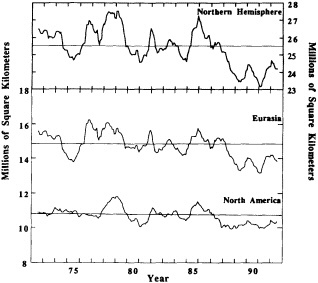
FIGURE 3
Twelve-month running means of snow cover over Northern Hemisphere lands (including Greenland) for the period January 1972 through December 1992. Running means are also shown for Eurasia and North America (including Greenland). Values are plotted on the seventh month of the twelve-month interval.
CONCLUSIONS
Significant strides have been made in recent years in the recovery, digitization, and validation of in situ observations of snow cover and their assimilation into regional networks. The availability of this information, in some cases going back to the turn of the century, complements the more recent global monitoring of snow from satellites. Analyses of both in situ and satellite observations show a considerable amount of year-to-year variability in the duration of snow cover on local to hemispheric scales. However, it is beginning to be recognized that this variability is often embedded in longer-term fluctuations. In situ data from the central United States points to multi-decadal fluctuations in the duration of snow over the past century, and the hemispheric satellite observations suggest variations lasting on the order of several years.
Efforts must continue to ensure the recovery and digitization of all available historic in situ observations, from both stations and snow courses. On the satellite side, the NOAA weekly product must continue to be produced in its present form. To abruptly or, perhaps more seriously, subtly alter the manner in which these charts are produced would severely weaken what is at present the longest and most consistent satellite-derived data set for any surface or atmospheric variable. Coincident with this must be efforts to improve the hemispheric monitoring of snow from microwave data using composited regional algorithms. Ultimately the goal must be to integrate all surface and satellite sources in a series of products reporting snow extent, depth and water equivalent, and regional surface albedo. These data should cover not only Northern Hemisphere lands but also lands in the Southern Hemisphere, ice sheets, and sea ice. Means
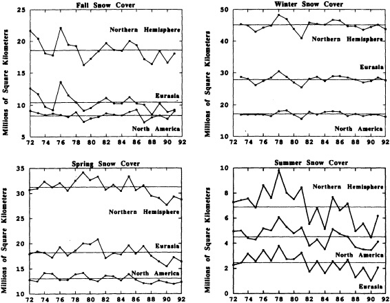
FIGURE 4
Seasonal time series of snow cover over Eurasia and North America (Greenland is excluded).
of integrating satellite and integrative products with earlier in situ observations must also be improved to provide the longest, most consistent records possible.
With adequate data available to analyze, knowledge of the spatial and temporal kinematics of snow cover over recent decades or even the past century will continue to improve. This will contribute to a better understanding of the role of snow in the climate system and to the utility of snow as an indicator of climate change.
ACKNOWLEDGMENTS
Thanks to G. Stevens at NOAA for supplying digital snow data and to A. Chang at NASA for providing microwave data. Thanks also to A. Frei, M. Hughes, and J. Wright at Rutgers for technical assistance. This work is supported by NOAA under grant NA90AA-D-AC518, and by the Geography and Regional Science Program of the National Science Foundation under Grant SES-9011869.
Variability and Trends of Precipitation and Snowfall over North America
PAVEL YA. GROISMAN1 AND DAVID R. EASTERLING2
ABSTRACT
Biases and large-scale inhomogeneities in the time series of measured precipitation and snowfall over the continent are discussed and analyzed. After adjustments and selection of the ''best" network, reliable "first guess" estimates of North American snowfall and precipitation have been obtained. Century-long time series of unbiased annual precipitation over the regions to the south of 55°N, and 40-year time series of unbiased area-averaged annual precipitation and snowfall for all of North America, have been developed. Analysis of the trends shows that:
-
During the last hundred years, annual precipitation has increased in southern Canada (south of 55°N) by 13 percent and in the contiguous United States by 4 percent to 5 percent; the main domain of this century-scale precipitation increase, however, is eastern Canada and the adjacent northern regions of the United States.
-
An increase of up to 20 percent increase in annual snowfall and rainfall has occurred during the last four decades in Canada north of 55°N.
INTRODUCTION
During the last century, global surface air temperature has increased approximately 0.5°C (over Canada it has been about 1°C); the seven warmest years in the instrumental records of global temperature occurred during the last decade (Budyko and Izrael, 1987; Gullett and Skinner, 1992; IPCC, 1990, 1992). With such a large change in the earth's heat balance, we suspect that changes in the water balance of North America may have also occurred. Given the potential for even greater changes over the next decades, there is an urgent need to obtain reliable results on North American precipitation changes during the last century.
Numerous studies have been made of precipitation over North America and the problems associated with precipitation measurement. The results of these studies can be summarized by saying that no definite century-scale precipitation trends have been found for the United States. (Canadian precipitation cannot be analyzed for the entire century,
due to lack of data in the northern part of the country.) Fluctuations on decadal time scales are evident, however, which led Klugman (1983) to claim "evidence of climatic change" in the U.S. seasonal precipitation during the 19481976 period. Diaz and Quayle (1980) found large-scale changes in contemporary precipitation (1955-1977) as compared to precipitation at the beginning of the century (1895-1920), but these changes were shown to be mainly statistically non-significant. Vining and Griffiths (1985) found an increase over time in the decadal variance of annual precipitation at 10 long-term U.S. stations for the period 1900-1979. Bradley et al. (1987), analyzing the area-averaged percentile of the U.S. annual precipitation, found a precipitation decrease during the period from the 1880s to the 1930s and a general increase thereafter.
There are several reasons for precipitation undercatch by the standard gauges currently being used worldwide (Bogdanova, 1966; WMO, 1991; WWB, 1974). The main factor that reduces the amount of measured precipitation as compared to "ground truth" is wind-induced turbulence over the gauge orifice (Sevruk, 1982). The absence of a wind shield for the gauge (or its poor design) makes the problem even more severe. Field experiments show that an appropriate wind shield (such as the modified Nipher shield used in Canada) reduces wind-related bias in the gauge catch to manageable levels that can then be easily adjusted. All elevated snow gauges in Canada have wind shields, but only about 200 of the approximately 6,000 U.S. gauges that report daily precipitation have a wind shield (Karl et al., 1993a). Furthermore, the Alter shield in use at U.S. stations provides less protection than the Canadian shield (Goodison et al., 1981). As a result, the existing U.S. rain-gauge network measures rainfall with a bias of 3 to 10 percent (Golubev et al., 1992; Sevruk and Hamon, 1984) and snowfall with a bias of up to 50 percent or more (Goodison, 1978; Larkin, 1947; Larson and Peck, 1974). Moreover, in Alaska total biases up to 400 percent in measurements of water equivalent of snowfall have been reported (Black, 1954).
Rain gauges at some of the U.S. primary stations were equipped with the Alter wind shields toward the end of the 1940s. The addition of the wind shield introduced an inhomogeneity into the time-series precipitation data at these stations. Although the stations with Alter shields constitute a small percent of the U.S. stations, they comprise 40 percent of the U.S. National Weather Service stations transmitting meteorological observations over the Global Telecommunication System (GTS) for publication in the Monthly Climatic Data for the World.
Canadian methods of making precipitation measurements differ significantly from those used in the United States. This is illustrated by the jump in measured precipitation values often registered by stations on opposite sides of the border between the two countries (WMO, 1979; WWB, 1974). Although the difference in liquid precipitation is small—the Canadian gauge typically measures a few percent more rain than the standard U.S. gauge (Sanderson, 1975)—there is a considerable difference in the solid precipitation measurements (Goodison et al., 1981; Sanderson, 1975). Currently, 85 percent of the Canadian meteorological network uses a 10:1 ratio as a measure of the water equivalence of fresh-fallen snow. Since the 1960s, 15 percent of this primary network has used an elevated snow gauge with a modified Nipher wind shield. This gauge catches solid precipitation effectively even during high-wind conditions (Goodison, 1978; Goodison et al., 1992). Its record differs systematically from the snow-stick measurements continued at other stations (Goodison et al., 1981; Groisman et al., 1993; Karl et al., 1993a). This difference in snow-measurement methods causes both space and scale inhomogeneities, which cannot be avoided by users of such international publications as World Weather Records and Monthly Climatic Data for the World, since Canada transmits only the data from its primary network over the GTS.
When point precipitation measurements are expanded to area-averaged values in rough terrain, the point values are often less than the "ground-truth area mean", because most meteorological stations are located in valleys, but the vertical gradients in precipitation have been neglected. Figure 1 shows two maps of annual precipitation over North America. The first map (la), which was constructed during the World Water Balance studies (1974), incorporates estimates of topographic effects on precipitation. However, the second map (lb) simply uses data from 1,900 stations, without any consideration of topographic effects on precipitation. Precipitation in the mountainous West is obviously underestimated on the second map, and even Appalachian-ridge precipitation estimates are noticeably biased.
The area-averaged annual precipitation value for the contiguous United States derived from Figure 1a is about 880 mm, while the value from Figure 1b is 700 mm. When we use data from all 6,000 U.S. cooperative stations, this latter annual total increases to 735 mm (NCDC, 1991) but still remains quite low compared to the value reflecting topography. The same problem has been revealed to exist for Canada by Hare (1980), who showed that annual totals over the country should be increased by 20 percent, on average, to obtain a reliable water balance (i.e., runoff = precipitation - evaporation).
Precipitation measurements are very sensitive to changes in the environment surrounding the gauge, in the gauge type, and in the methods of measurement. A small move of the gauge can result in a twofold change in the values of measured precipitation if the gauge exposure is changed (Karl et al., 1993b; Sevruk, 1982). After spatial averaging, it can be expected that the random errors connected with such shifts will cancel out. However, when systematic changes occur countrywide, they cannot be assumed to cancel out. Several such changes have occurred during the
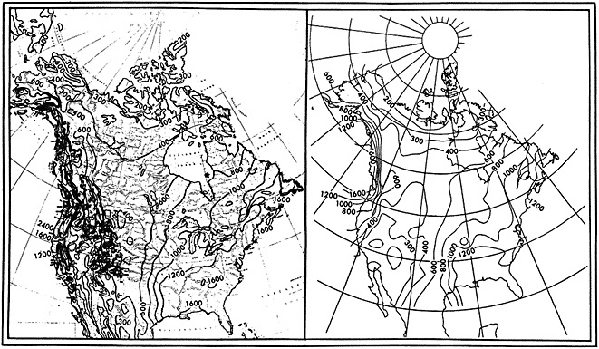
FIGURE 1
Mean annual precipitation over North America: left panel, from WWB (1974); right panel, as estimated using the meteorological network.
last century in the Canadian and the U.S. meteorological primary networks (Figure 2). Area-averaged precipitation time series are especially sensitive to such large-scale inhomogeneities because their noise component has been decreased by averaging. Therefore, when studying trends in these time series, we must be sure that the observed large-scale decadal changes represent true climatic changes rather than artificial changes introduced into the network. Any analysis of precipitation over North America should be preceded by a thorough analysis of the history of observations in the network. This analysis should be followed by selecting a subset of the "best stations" and applying adjustments to the initial data to compensate for all known large-scale inhomogeneities. Our analyses in the following sections give special attention to the selection of the precipitation data and to the adjustments to be made to them.
DATA SELECTION AND PROCESSING
Networks Used
In our studies of precipitation over North America, we selected several networks, each with a special purpose in mind. Figure 3a shows the network that was used to study snowfall. It consists of 223 U.S. first-order stations (including Alaska) and 1,107 Canadian stations selected using the requirement that each station have data available for at least 15 years out of the last two decades. The period 1950-1990 was chosen because by then all U.S. first-order stations had been relocated to airports with relatively open sites, and because the networks for northern Canada and Alaska had become dense enough to assure adequate spatial sampling only after World War II. A reliable analysis of changes in snowfall and total precipitation over the entire continent could thus be made only for the last 40 years.
Since the 1960s there have been parallel observations of snowfall (by stick measurements) and its water equivalent (measured by elevated snow gauges) at 335 Canadian stations. These observations were used to evaluate the adjustments made by Groisman (1992) and Karl et al. (1993a) to homogenize time series of solid precipitation in Canada.
Figure 3b shows the network that was used to study century-scale changes of annual precipitation over the contiguous United States and southern Canada. It consists of the same Canadian stations, 45 cooperative Alaskan stations, and 593 "best" cooperative stations selected from the U.S. Historical Climatology Network (Karl et al., 1990). The U.S. stations were selected on the basis of the length of their records (they all began their observations in the nineteenth century) and their having had few station moves or other
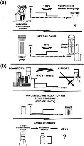
FIGURE 2
Sketch of the history of precipitation measurement in North America related to precipitation time-series homogeneity. Major large-scale changes caused inhomogeneities in these time series. (a) Canadian primary network; (b) U.S. primary network.
obvious sources of inhomogeneities. The data are therefore free of the large-scale inhomogeneities shown in Figure 2, but other inhomogeneities may still exist.
The Canadian network, which seems quite large in Figure 3b, declined rapidly in size during the first half of the century (see Table 1). In southern Canada it contained only 190 stations by 1940, and 26 stations in 1900. As a consequence, we selected a special network of Canadian stations that were operating in the 1920s (Figure 3c) to use in to studying Canadian precipitation prior to World War II. The area-averaged precipitation time series based on this network were combined with the corresponding time series developed from the main network shown in Figure 3b.
Data Processing
The precipitation data for the 593 contiguous U.S. stations and the snowfall data were used without adjustments.
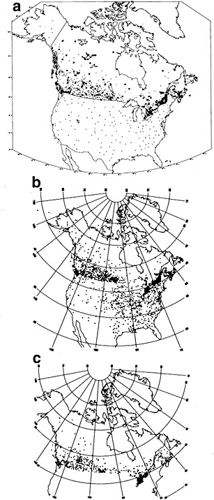
FIGURE 3
Stations used in this paper for analysis of: (a) snowfall (squares depict the primary Canadian stations where the elevated snow gauges were installed in the 1960s); (b) precipitation; (c) accuracy of precipitation changes in southern Canada before World War II.
TABLE 1 Number of Stations with Available Data on Annual Precipitation for Southern Canada
|
|
Year |
||||||
|
Data Set |
1895 |
1910 |
1925 |
1940 |
1955 |
1990 |
Total |
|
Main data set used in the study |
22 |
35 |
119 |
190 |
315 |
765 |
995 |
|
Alternative set of Canadian stations with observations prior to 1925 |
54 |
86 |
323 |
261 |
162 |
24 |
385 |
|
All Canadian stations with observations prior to 1925 |
70 |
117 |
439 |
384 |
277 |
133 |
523 |
The Canadian rainfall data were corrected for the gauge change that occurred in the mid-1970s. All rainfall data before 1975 were increased by a factor of 1.025 to approximate the results of Goodison and Louie (1986).
To obtain the water equivalence of snowfall at the Canadian stations, we were able to derive scale adjustments from the set of parallel observations made at the Canadian stations depicted in Figure 3a (full squares). These adjustments reduce snow-stick measurements to match the records of the elevated snow gauge. However, these records still need some corrections for the type (or absence) of wind shield (Goodison, 1978). Larger corrections are required for the U.S. rain gauges (Larson and Peck, 1974; Goodison and Metcalfe, 1989; Peck, 1991) because these gauges do not have wind shields. We hope to be able to use such corrections in the future, but for the moment we can only conclude that the discontinuity across the border of the two countries in measured water equivalent of snowfall is caused by significantly biased measurements in the U.S. data. Therefore, area-averaging of annual precipitation over the regions encompassing both Canada and the United States was done separately for each country. Only snow-stick measurements were used to represent the Canadian solid precipitation. Each area-mean time series was adjusted to its unbiased precipitation value (using the method described by Groisman et al. (1991), which relies on the WWB (1974) estimates of long-term annual precipitation shown in Figure 1a); then time series from the two parts of the region were combined. Furthermore, we prefer to consider the southern Canadian regions separately, due to the instability of their data coverage.
As noted earlier, Table 1 shows the rather variable number of stations providing annual-precipitation data for southern Canada (south of 56°N) for the two non-interlaced networks shown in Figures 3b and 3c. Figure 4 shows time series of annual snowfall and total precipitation area-averaged over Canada south to 55°N, based on these two independent data sets. There is little difference between them during the twentieth century, which confirms the accuracy of the area averaging and the representativeness of the network used. The only noticeable difference is in the 1890s, when precipitation data were available for only 20 to 30 stations over the main network. Hence, we combined these two networks to develop a century-long area-averaged time series of southern Canadian precipitation. The time series for the period 1891-1960 were developed from the network of stations shown in Figure 3c, together with those stations from the main Canadian network that were operating prior to 1925. These time series were combined with the time series for the period 1921-1990 that was based on the data of the 1,107 stations.
Snowfall Scale Correction
In developing the data set used to construct unbiased area-averaged snowfall time series (Figure 5), we made one
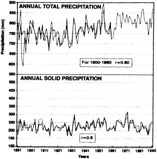
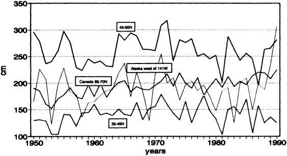
FIGURE 5
Annual snowfall over North America during the last 40 years. The applied scale-correction factors for network elevation are: for Alaska—1.23; for Canada, Zone 55-70°N—1.14, Zone 45-55°N—1.19, and Zone 35-45°N—1.47.
important scale correction that was not performed in the work of Karl et al. (1993a). Bogdanova (1977) showed that in mountains the mean long-term ratio of solid to total annual precipitation rises at a mean rate of 27 percent per 1000 m. We used this to adjust the snowfall time series for network elevation. Without this adjustment, the biases in the regionally averaged snowfall values would be very large. Table 2 provides the mean elevation of the network depicted in Figure 3b, together with true mean surface elevation for large regions of the United States and Canada (the mean elevation of the networks depicted in Figures 3a and 3b scarcely differ). From this table it is clear that with our network it would be possible to estimate occurrence of
TABLE 2 Mean Elevations of Meteorological Stations in the United States (Historical Climatology Network) and Canada Versus Real Surface Elevations*
|
|
Elevation, m |
|
|
Region |
Network |
Surface |
|
Western United States** |
790 |
945 |
|
Eastern United States |
145 |
235 |
|
Canada |
305 |
490 |
|
Alaska west of 141°W |
100 |
510 |
|
* Real surface elevations were estimated from NGDC (1988) data with 5-degree resolution ** "Western" and "Eastern" here refer to west or east of a line drawn from New Orleans to Detroit |
||
traces of snowfall only in the valleys and on the plains of western United States, and completely miss its mountainous portion. So our snowfall adjustment for each region was evaluated in the following way:
-
The mean long-term ratio of solid to total annual precipitation (rat1) was estimated for a plane with the elevation of the network depicted in Figure 3a.
-
This ratio was increased using a coefficient of 27 percent km-1 to obtain its value (rat2) for a plane with the elevation corresponding to the true surface elevation of the region.
-
The value of the estimated area-averaged snowfall was then multiplied by an adjustment scale coefficient equal to rat2 divided by rat1.
These coefficients were used for every graph in Figure 5. They are, however, conservative estimates of the adjustment needed if indeed the total precipitation area-averaged over the whole region depends on true surface elevation rather than on the elevation of the network used ( Karl et al., 1993a).
In the following section, area-averaging by the polygon method (Kagan, 1979; Thiessen, 1911) and scale correction (Groisman et al., 1991) were used in to develop regional, unbiased century-scale annual precipitation time series for the contiguous United States and southern Canada, together with 40-year time series of snowfall and total precipitation over all of North America. So that missing data would not affect the results, we averaged the anomalies from the reference period 1971-1990 and then reconstructed the area-averaged precipitation, adding the corresponding area-
averaged value of the mean precipitation for the same reference period. (While processing the data of the Canadian network that was operating in the 1920s, we used the reference period 1921-1940.) These time series provide our first approximation of contemporary changes of North American precipitation. The first experiments using individual gauge corrections (Groisman, 1991) showed that this approximation does not change substantially on a continental scale after the intra-annual variability in gauge errors has been taken into account.
CURRENT CHANGES IN PRECIPITATION AND SNOWFALL
Snowfall Changes During the Last Four Decades
Figure 5 shows the zonally averaged snowfall over Alaska, Canada north of 55°N, and the zones 45°N to 55°N and 35°N to 45°N for the last four decades. The basic statistics of these time series appear in Table 3.
When the spatial correlation function is known, the accuracy of area averaging over these regions using the networks depicted in Figure 3 can be estimated. The method of estimation, which was developed by R.L. Kagan (1979), can be applied to every isotropic two-dimensional field. In North America we used this method only for northern Canada. Since even today the meteorological network in northern Canada is relatively sparse, we had to estimate the representativeness of the network beforehand in order to analyze the changes over this area.
The spatial correlation function for northern Canadian snowfall can be approximated by the relationship r(R) =![]() , where R is the distance; R0 = 710 km, the radius of correlation; and C = 0.84. The value of (1-C)/C, which equals 0.19, is a measure of the error of measurements combined with microscale snowfall variability near the stations (Kagan, 1979). For the network selected, the mean-square error of spatial averaging of annual snowfall over northern Canada was estimated to be 17 percent of the theoretical variance of the area-averaged snowfall time series in the first half of 1950s; during the period 1956-1990 the error was about 10 percent. The number and spatial distribution of snowfall-measuring stations for southern Canada and the United States during the last four decades were adequate, so there was no need to verify the representativeness of the area-mean values.
, where R is the distance; R0 = 710 km, the radius of correlation; and C = 0.84. The value of (1-C)/C, which equals 0.19, is a measure of the error of measurements combined with microscale snowfall variability near the stations (Kagan, 1979). For the network selected, the mean-square error of spatial averaging of annual snowfall over northern Canada was estimated to be 17 percent of the theoretical variance of the area-averaged snowfall time series in the first half of 1950s; during the period 1956-1990 the error was about 10 percent. The number and spatial distribution of snowfall-measuring stations for southern Canada and the United States during the last four decades were adequate, so there was no need to verify the representativeness of the area-mean values.
The accuracy of area averaging of the data in northern Canada is high enough to confirm the strong positive linear trend in annual snowfall revealed in the zone (19 percent over four decades). This trend, in conjunction with the trend in rainfall data (not shown), confirms the systematic increase in annual totals of precipitation during the entire period of instrumental observations.
Snowfall in the zone 45°N to 55°N is closely connected to temperature changes on continental and hemispheric
TABLE 3 Statistical Characteristics of Time Series (1950-1990) of Annual Snowfall and Total Precipitation Zonally Averaged over North America (see Figures 5 and 6)
|
Annual Snowfall |
|||
|
Mean and Standard Deviation, in cm |
|||
|
Region |
Mean |
Std. Deviation |
Linear Trend ± its Standard Error, in % per Decade |
|
Alaska |
190 |
35 |
2.7 ± 2.5 |
|
Canada, zone 55-70°N |
195 |
17 |
5.1 ± 0.8 |
|
Canada/U.S., zone 45-55°N |
260 |
27 |
-0.7 ± 1.4 |
|
U.S./Canada, zone 35-45°N |
140 |
18 |
1.8 ± 1.7 |
|
Total Precipitation |
|||
|
Mean and Standard Deviation, in mm |
|||
|
Region |
Mean |
Std. Deviation |
Linear Trend ± its Standard Error, in % per Decade |
|
Alaska |
510 |
59 |
2.7 ± 1.5 |
|
Canada, zone 55-70°N |
495 |
33 |
4.2 ± 0.6 |
|
Canada/U.S., zone 45-55°N |
940 |
41 |
0.7 ± 0.6 |
|
Canada/U.S., zone 35-45°N |
905 |
66 |
1.9 ± 0.9 |
|
United States, zone 28-35°N |
1175 |
137 |
3.4 ± 1.5 |
scales; the correlation between this time series and the annual mean surface air temperature over the Northern Hemisphere is about -0.7 (Groisman et al., 1993). Using this relationship, and taking into account the intrinsic coherence of annual snowfall totals in southern Canada (which encompasses the main part of the 45°N to 55°N zone) with regional maximum temperature (Groisman, 1992), we could expect a future decrease in snowfall for this zone if the global warming projected by IPCC (1990) actually occurs.
We realize that the large adjustment coefficient for zonal snowfall in the 35°N to 45°N zone (1.47), while providing a more realistic mean value, cannot be considered a satisfactory solution to the problem of snowfall changes over this zone. Unfortunately for the current concerns about potential climatic change, we still do not have a reliable source of data on the snowfall over the main part of the United States.
Annual Precipitation Changes During the Last Four Decades
Figure 6 shows the unbiased annual precipitation totals for the last four decades, area-averaged over the same four zones used in Figure 5 plus the southern part of the United States (a zone from 28°N to 35°N and to the east of 105°W). The basic statistics of these time series appear in Table 3. It can be seen from this table that annual precipitation has increased during these last decades over the entire continent, but especially significantly over the southeastern United States (14 percent per 40 years) and northern Canada (17 percent per 40 years).
Century-Long Precipitation Changes
Table 4 (adapted from Groisman, 1992) provides the same characteristics as in Table 3 for the century-scale precipitation changes over southern Canada and the contiguous United States. This table confirms the main conclusions derived from Table 3, but shows that, as with the U.S. precipitation, it is unwise to discuss the statistical significance of precipitation trends on the basis of the 41-year record alone (on the century scale the linear trend is not statistically significant).
Given the major terms of the water-balance equation, we can assume that, in general, the variability of annual precipitation drives the variability of annual stream flow (Linsley et al., 1958). Streamflow will thus have approximately the same large-scale features and areas of coherent change as the precipitation used to estimate it. The stream flow data are independently collected and do not exhibit the errors and data problems mentioned in previous sections (they have their own problems and errors, but do not suffer from the rain-gauge problem; being natural area averages, they give representative estimates of changes in the hydrological cycle of the regions under consideration. Therefore, in our study of the spatial correlation of the precipitation field over North America, we divided the area into several homogeneous regions on the basis of the results of a principal component analysis of stream flow data for the United States made by Lins (1985). In his analysis, Lins used a dense network of small watersheds not disturbed by anthropogenic activity. He evaluated five principal components,
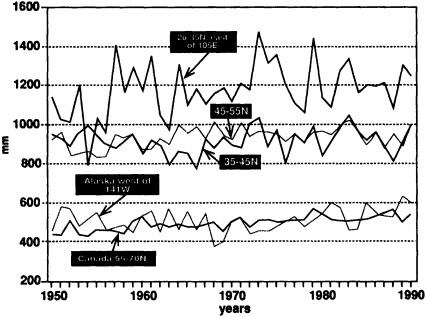
FIGURE 6
Annual precipitation over North America during the last 40 years.
TABLE 4 Statistical Characteristics of the Century-long Time Series of Annual Precipitation, Area-Averaged Over Canada South of 55°N and the Contiguous United States
|
Mean and Standard Deviation, in mm |
|||
|
Region |
Mean |
Standard Deviation |
Linear Trend ± its Standard Error, in % per 100 yrs |
|
Southern Canada |
925 |
56 |
13.3 ± 1.7 |
|
Contiguous United States |
870 |
66 |
4.5 ± 2.6 |
each with a distinctive regional pattern: south-central United States, northwestern United States, southwestern United States, north-central United States, and northeastern United States. The generalized map of these regions expanded on the Canadian territory up to 55°N is shown in Figure 7.
In order to identify the independent components of the precipitation pattern, we applied the spatial averaging to the regions depicted in Figure 7. Time series of adjusted annual precipitation area-averaged over these five regions are shown in Figure 8; their correlation matrix appears in Table 5, and their main statistical features in Table 6. From Table 5 we can see that the time series from the different regions are not closely correlated (the north-central region correlated best with other regions, since it has a common border with each of them). Hence, we can analyze and describe each time series separately.
The debiasing procedure used (Groisman et al., 1991) does not affect trends, but it does change the scale of the time series. For Canada and eastern United States, the corresponding scale factors are not large; they vary from 1.05 (south-central region) to 1.25 (northeastern region). However, in the western United States they become larger (1.5 for the southwestern region and 1.7 for the northwestern United States). This shows that even annual totals are not well measured by the existing meteorological network.
An increase of more than 10 percent per century in annual precipitation over southern Canada (Table 4) is reflected by a corresponding precipitation increase over the northeastern
TABLE 5 Correlation Matrix of the Area-Averaged Century-long Time Series of Annual Precipitation Depicted in Figure 8
|
U.S. Region* |
N-West |
N-Central |
N-East |
S-West |
S-Central |
|
Northwestern |
1.00 |
0.44 |
0.26 |
0.23 |
0.16 |
|
North-central |
|
1.00 |
0.29 |
0.28 |
0.38 |
|
Northeastern |
|
|
1.00 |
0.08 |
0.11 |
|
Southwestern |
|
|
|
1.00 |
0.11 |
|
South-central |
|
|
|
|
1.00 |
|
* See Figure 7 for a depiction of these regions |
|||||
TABLE 6 Statistical Characteristics of the Area-Averaged Century-long Time Series of Unbiased Annual Precipitation Depicted in Figure 8
|
|
Mean and Standard Deviation, in mm |
Linear Trend ± its Standard Error, in % per 100 yrs |
|
|
Region* |
Mean |
Standard Deviation |
|
|
Northwestern |
825 |
70 |
5.5 ± 2.9 |
|
North-central |
845 |
65 |
12.1 ± 2.4 |
|
Northeastern |
1265 |
90 |
11.3 ± 2.2 |
|
Southwestern |
515 |
90 |
0.5 ± 6.1 |
|
South-central |
1115 |
110 |
5.4 ± 3.4 |
|
All Five Regions Together |
925 |
55 |
7.6 ± 1.9 |
|
* See Figure 7 for a depiction of these regions |
|||
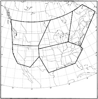
FIGURE 7
Regions over North America (south of 55°N) with spatially homogeneous patterns of stream flow (based on principal-component analysis by Lins (1985)) extended to southern Canada.
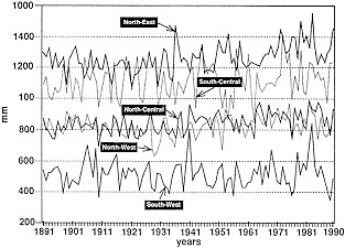
FIGURE 8
Century-long annual precipitation changes over the United States and southern Canada, area-averaged over the five regions depicted in Figure 7.
and north-central regions. Linear trends account for up to 20 percent of the variance of annual precipitation over each of these two regions. However, the trends of 5 to 6 percent per century documented for northwestern and south-central regions are not statistically significant at the 0.05 level, and there have been no systematic changes over the southwestern region during the last 100 years. Therefore, we can conclude that during the last century a large-scale increase has occurred over all of North America, but that the major source of this increase was changes in eastern Canada and adjacent regions of the United States (the northeastern quarter of the country).
CONCLUSIONS
Standard rain gauges installed at the U.S. and Canadian meteorological networks undercatch "true" precipitation, especially in its solid form. The biases induced by this undercatch have altered during the last century, due to changes in instrumentation and measurement practices. This introduces large-scale inhomogeneities in the time series of the precipitation field over the continent. Climatological studies that do not take into account these inhomogeneities will give misleading results. The low-elevation locations of the existing meteorological network necessitate further research to determine reliable estimates of snowfall changes over the United States. Problems also exist in estimation of total precipitation in the mountainous west of the continent. The scale corrections, which transform area-averaged precipitation data into the unbiased values of "ground true" regional precipitation, increase precipitation estimates in that region by up to 70 percent. These uncertainties in the data restricted our analysis to spatially averaged values of annual precipitation and snowfall over large regions.
After adjustments and selection of the "best" network, reliable "first guess" estimates of North American snowfall and precipitation were obtained. Century-long time series of unbiased annual precipitation over the regions to the south of 55°N, and 40-year time series of unbiased area-averaged annual precipitation and snowfall for all of North America, were developed. Analysis of the trends shows that:
-
During the last hundred years, annual precipitation has increased in southern Canada (south of 55°N) by 13 percent, and in the contiguous United States by 4 to 5 percent.
-
An increase of up to 20 percent in annual snowfall and rainfall has occurred during the last four decades in Canada north of 55°N.
-
In the zone 45°N to 55°N, century-scale total precipitation has increased, while a redistribution between the solid and liquid forms has occurred coherently with variation of the zonal maximum temperature (and global surface air temperature).
-
The main domain of the century-scale precipitation increase over North America to the south of 55°N (to the north of this latitude the data for the first half of the century are absent) is eastern Canada and adjacent northern regions of the United States.
ACKNOWLEDGMENTS
This paper was completed while the first author worked as a National Research Council senior research associate
at the U.S. National Climatic Data Center. Support for David R. Easterling was provided under Department of Energy (DOE) Interagency Agreement DE-A105-90ER60952 and NOAA's Climate and Global Change Program.
Commentary on the Paper of Groisman and Easterling
DAVID A. ROBINSON
Rutgers University
I think Dr. Groisman's presentation has been an excellent example of the advantages and pitfalls of dealing with observational data and of putting data together on a variety of temporal and spatial scales. And I can assure you that the paper contains some tremendous information that, unfortunately, Dr. Groisman had time only to gloss over. I would like to break the study down into a couple of segments to foster further discussion.
The first section I shall simply entitle ''obtaining numbers". This includes the problems Dr. Groisman presented that relate to measurement techniques, whether for obtaining liquid rainfall or, more important, getting adequate snowfall measurements. Next, there are the problems in developing an observational network that is homogeneous through time—which, as Dr. Groisman found, was impossible to do for the entire North American continent. He could look only at the southern reaches of Canada and over the United States for the entire century. When it came to looking into the Arctic, he could go back only about 40 years.
Third is the paper's serious criticism, which may have passed people by too quickly, that it is difficult to believe anything that comes out of the primary stations in the United States. The figure that shows the changes at these stations (relocation, gauge changes, wind shields) really substantiates that. So we essentially have different observational networks that vary through time.
Last, there is the whole idea of metadata. We must have enough information on the history of a station or network that we can go back and reconstruct a homogeneous, standardized time series over decade-and century-long periods. While North American metadata is certainly better than African, there are gaps and lapses in the station histories. For precipitation, the impact of station moves is less significant than for temperature. But the gauges that measure precipitation, the wind shields, the 8-inch gauge versus the tipping bucket, and so forth are as important as any problems in measuring temperature in the United States.
It occurs to me to wonder how Dr. Groisman would rank these concerns in terms of importance for obtaining homogeneous precipitation records. To me, the most significant problem is perhaps the switch to the tipping bucket with the introduction of automated surface observing systems at primary U.S. observing stations over the next few years. Some time down the road when we are looking for decadal variations in precipitation, we may have to examine the metadata for the 1990s very carefully to come up with a homogeneous time series.
Another question I have is how deeply inhomogeneities interfere with obtaining true signals. You have to do so much with the data to be able to compare it at different times at an individual station, or among stations or countries. How deeply does this limit our ability to recognize climate change? Tom Karl et al. stated in their 1991 Science paper that it would take several decades to recognize a change in precipitation over central North America that might be an anthropogenic signal. I wonder how much these inhomogeneities in the different gauges and the different national recording procedures would extend or contribute to that lag, particularly when it comes to a noisy record like precipitation.
When it comes to point-to-area transformations, the question is where to draw the line. Dr. Groisman has done a lot of extrapolation, particularly in the western reaches of North America, in order to take into account elevational factors or orographic factors for precipitation. In some cases factors as great as a 70 percent increase were applied to the precipitation results of station networks. At some point one must decide whether to stay with point data, or at least data from a similar elevational area, or to stretch and extrapolate the data in order to obtain a more spatially complete and, in terms of absolute values, a more accurate record. Dr. Groisman did make it clear that the extrapolation does not interfere with any type of trend analysis; my question relates only to the absolute values of precipitation and snowfall generated.
Now for evaluating the numbers. Let us begin with the climatologies of snowfall and precipitation. It was interesting that at a given point in time when there was a larger mean, the standard deviations increased. When it comes to climate change, it is important to know whether we see a change in the mean or a change in the variability of climate.
Next Dr. Groisman looked at time series: the 40-year variety, the 100-year variety, precipitation, snowfall, Alaska, Canada, and the lower 48. There are so many interesting things in these time series-for instance, the major increase in snowfall in the Alaskan time series in the 1980s. Is
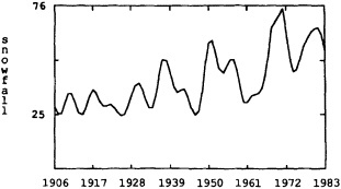
FIGURE 1
Smoothed time series of winter (December to February) snowfall in cm at Napoleon, North Dakota. Data from 1902 through 1987 have been smoothed with a nine-point binomial filter; the only points plotted are those where 9 years are available for filtering (i.e., plotted year ± 4 yr).
this associated with what has been happening in the North Pacific? We know that the North Pacific was rather cool in the 1980s compared to most of the rest of the globe.
I would like to show a few time series of snowfall. The stations are from a network of about 1,000 stations—about 300 of which go back to the turn of the century—over the United States, which I have assembled and quality-controlled in cooperation with NCDC. Figure 1 looks at Napoleon, North Dakota for the past century. An important point here is that these are stick measurements of snowfall and snow depth. Thus, they have no biases due to a change of gauge. We have not yet applied filters and looked for decadal variations. But you can see the suggestion of an increase in snowfall at Napoleon during the century.
Figure 2 is a record of New Brunswick, New Jersey snow going back to 1860. This is not total snowfall, but the number of 5-inch-plus and 10-inch-plus snowfall events. You can see quite a bit of variation across time. I do not see anything in the way of trends or cycles. This small study was inspired by the fact that until March 18, 1992, it was the third least snowy winter in New Brunswick in the last 135 years. Then it snowed 10 inches in 4 days, shooting the near-record to pieces.
It is interesting to note from this figure that the 1973-1974 to 1990-1991 period was the longest interval in which not a single year missed having a 5-inch-plus snow event. The winter of 1991-1992 ended that string. Another item of interest is that in the past 135 years, no year has had more than five 5-inch-plus snow events in central New Jersey.
Another way of examining this time series is to sum the number of 5-inch (12.7 cm) snow events by decade, as in Table 1. Here you can see that the 1980s had the most 5 inch-plus snowfall events of any decade on record. I have shown this chart to people throughout New Jersey, and no one ever believes me. However, the subject of one's
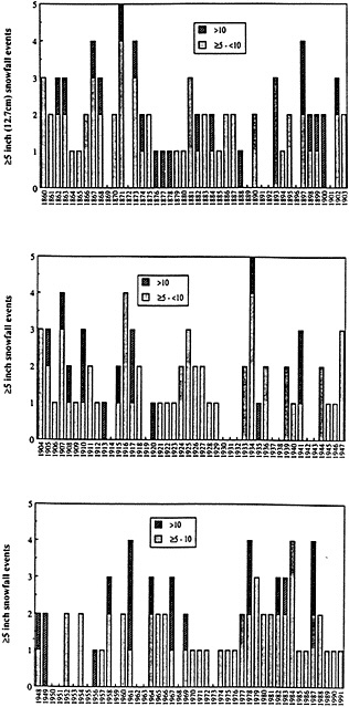
FIGURE 2
Number of =5-inch to <10-inch ( =12.7-cm to <25.4-cm) and =10-inch snowfall events per winter (October through April) from 1859/1860 to 1990/1991 at New Brunswick, New Jersey. (A snowfall event may be longer than one day, but may not be interrupted by a day without snowfall; no such events were observed for winter 1991/1992.)
perception of climate change is best left for discussion at another time.
Finally, Dr. Groisman talked about associations between snowfall, precipitation, and other climatic variables, and noticed that from 45°N to 55°N there was an inverse rela-
TABLE 1 Snowfall Events* in New Brunswick, N.J. by Decade, 1860-1989
|
|
Number of Snowfall Events* |
||
|
Decade |
=5" to <10" |
10" |
=5" |
|
1860s** |
18 |
4 |
22 |
|
1870s |
13 |
5 |
18 |
|
1880s |
13 |
3 |
16 |
|
1890s |
12 |
4 |
16 |
|
1900s |
15 |
6 |
21 |
|
1910s |
12 |
6 |
18 |
|
1920s |
14 |
1 |
15 |
|
1930s |
10 |
2 |
12 |
|
1940s |
10 |
5 |
15 |
|
1950s |
7 |
2 |
9 |
|
1960s |
11 |
7 |
18 |
|
1970s |
13 |
2 |
15 |
|
1980s |
19 |
4 |
23 |
|
Total |
167 |
51 |
218 |
|
* Snowfall event may be longer than I day, but may not be interrupted by a day without snowfall. ** Decade of the 1860s = winters 1859-60—1868-69. |
|||
tionship between temperature and snowfall. When examining Northern Hemisphere snow and temperature together, as shown in Figure 3, we have found that both are 12-month running means. The snow, which is from the NOAA
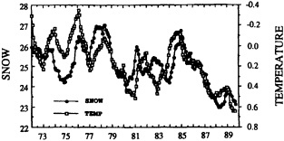
FIGURE 3
Twelve-month running means of snow cover, in millions of km2 and surface air temperature, in degrees Celsius, over Northern Hemisphere lands for January 1973 through August 1990. Temperatures are expressed as departures from the reference period, 1951-1970. Temperature data from P.D. Jones. From Robinson et al. (1991).
hemispheric snow charts, is a weekly product that we have averaged into monthly values. The temperature is Phil Jones's data set. Notice the striking relationship between hemispheric temperature—and that is from pole to equator—and Northern Hemisphere snow cover. We are beginning to examine snow and temperature by region and by season. So we see the same general association at this point, at least in a hand-waving sense, as Dr. Groisman found with the snowfall.
Discussion
RIND: You mentioned the relationship between precipitation over North America and global mean temperature. I wanted to add that the warming patterns for the 1930s and the 1980s were very different, just as you said the precipitation patterns were. The 1930s had very large warming at high latitudes with little effect at low latitudes, like an ocean heat-transport change pattern. The 1980s had very uniform warming as a function of latitude, more like what the models are projecting for CO2 and trace-gas forcing. They may be good examples of two different types of processes.
WALSH: That increase of snowfall in northern Canada is interesting in relation to the borehole measurements mentioned yesterday. If snowfall increases, it tends to insulate the ground during the coldest part of the year, which can complicate interpretation of borehole measurements. Also, perhaps we should take a closer look at how subsurface temperatures relate to snowfall to see what the implications might be of a continued increase in snowfall in permafrost areas.
TRENBERTH: The summer and winter correlations between precipitation and temperature tend to be very different.
GROISMAN: That's true. We simply wanted to create annual precipitation time series we could relate to some of the early data.
Asymmetric Trends of Daily Maximum and Minimum Temperature: Empirical Evidence and Possible Causes
THOMAS R. KARL1, PHILIP D. JONES2, RICHARD W. KNIGHT1, GEORGE KUKLA3, NEIL PLUMMER4, VYACHESLAV RAZUVAYEV5, KEVIN P. GALLO1, JANETTE A. LINDESAY6, AND ROBERT J. CHARLSON7
ABSTRACT
An examination of monthly maximum and minimum temperatures indicates that the rise of minimum temperature (0.84°C) has occurred at a rate three times that of rise of maximum temperature (0.28°C) over the period 1951 to 1990. This conclusion is based on data from over 50 percent (10 percent) of the Northern (Southern) Hemisphere land mass, accounting for 37 percent of the global land mass. The decrease of the diurnal temperature range is approximately equal to the increase of mean temperature. The asymmetry is detectable in all seasons in most of the regions studied.
The decrease in the daily temperature range is at least partially related to an observed increase in cloudiness. However, an empirical analysis of nearly 50,000 daily observations across 14 stations throughout the United States indicates that the daily temperature range is also sensitive to relative humidity, global radiation, surface stability, thermal advection, and snow cover; earlier work has shown that the temperature range is also sensitive to surface boundary conditions such as soil moisture. Locally, the diurnal range can also respond to increasing urbanization, irrigation, and desertification, but this effect appears to be small in our analysis.
Both general circulation models (GCMs) and radiative-convective models (RCMs) indicate that a decrease in the daily temperature range is likely with increases of CO2. The magnitude
of the range decrease simulated by GCMs, however, is only 10 percent of the magnitude of the simulated mean average temperature increase, whereas the observational record shows nearly equal changes of the daily temperature range and the mean temperature. The clear-sky daytime forcing by sulfate and carbonaceous aerosols, and other indirect effects such as increased cloudiness and albedo, operate in a sense that may reduce the daily temperature range; however, the decadal changes of this geographic and seasonally varying forcing are not well known. At present we do not have an adequate explanation for the observed decrease in the temperature range, or for the lack of daytime warming, yet these changes are clearly important, both scientifically and practically.
BACKGROUND
The mean monthly maximum and minimum temperature is derived from an average of the daily maximum and minimum temperatures. The monthly mean diurnal temperature range (DTR) is defined as the difference between the mean monthly maximum and minimum temperatures. The dearth of appropriate data bases that include information on the daily or mean monthly maximum and minimum temperature has previously impeded our ability to investigate changes in these quantities. The problem has historical roots. It arises because the climatological data that are made available internationally by national meteorological and/or climate data centers are usually derived from the monthly climate summaries (CLIMAT messages) on the Global Telecommunications System (GTS), which do not include information on the maximum or minimum temperatures. The GTS is the principal means by which near-real-time, in situ, global-climate data are exchanged. Moreover, the problem has been exacerbated because the World Meteorological Organization's retrospective data collection projects such as World Weather Records and Monthly Climatic Data of the World have always been limited to mean monthly temperatures. This has forced climatologists interested in maximum and minimum temperatures either to develop historical data bases on a country-by-country basis (Karl et al., 1991 a) or to try to work with the hourly GTS synoptic observations. The former is a slow, painstaking process, and the latter has been limited by poor data quality and metadata (information about the data) and records of short duration (Shea et al., 1992).
The first indication that there might be important large-scale characteristics related to changes of the mean daily maximum and minimum temperatures was reported by Karl et al. (1984a). Their analysis indicated that the DTR was decreasing at a statistically significant rate at many rural stations across North America. Because of data accessibility problems, subsequent empirical analyses continued to focus on data from North America over the next several years (Karl and Quinn, 1986; Plantico et al., 1990). By 1990, however, a United States/People's Republic of China (PRC) bilateral agreement organized by the U.S. Department of Energy and the PRC Academy of Sciences provided the opportunity to analyze maximum and minimum temperatures from the PRC. Also about this time, the Intergovernmental Panel on Climate Change (IPCC) made arrangements with the Australian National Climate Centre to analyze maximum and minimum temperature data from southeastern Australia. The IPCC (1990) reported a significant decrease in the DTR from both of these regions. Meanwhile, work from another data exchange agreement, a bilateral between the United States and the former Soviet Union, came to fruition as a data set of mostly rural maximum and minimum temperatures was developed for the former Soviet Union. Karl et al. (1991a) reported on the widespread decrease of the DTR over the former Soviet Union, China (not including Tibet), and the contiguous United States, as was highlighted by the IPCC (1992).
Additional data from other countries and updates to previous analyses have now been analyzed. Data from the eastern half of Australia, Canada, Alaska, Sudan, Japan, some Pacific island stations, South Africa, and a few other long-term stations in Europe have now been included. Figure 1 shows the area of the globe that has now been analyzed for differential changes of the maximum and minimum temperature. This area now covers over 50 percent of the Northern and 10 percent of the Southern Hemisphere land masses, but still only about 37 percent of the global land mass.
FIGURE 1
Areas of the globe (indicated by shading) that have been analyzed in this paper for changes of mean maximum and minimum temperature.
OBSERVED CHANGES OF MEAN MAXIMUM, MINIMUM, AND DIURNAL RANGE
Spatial and Seasonal Patterns of Contemporary Trends
Daily maximum and minimum temperatures from over 2,000 stations were available for analysis in the countries shaded in Figure 1 during the period 1951 to 1990 (except for Sudan and the former Soviet Union, which had data through 1987 and 1989, respectively). Selected subsets of these data were averaged within various regions of each country. The definition of each region represents a compromise between climatic homogeneity and ensuring an adequate number of stations within its boundaries to limit sampling error. The base period for calculating departures from the average included the years 1951 to 1990 (or slightly fewer years in some countries, as mentioned before). The regions are delineated in Figure 2 where, as in other large-scale studies of the change of the mean annual temperature (Jones et al., 1986a,b; Jones, 1988), the average of the trends of the mean annual maxima and minima reveals a general rise of temperature. A decrease of the minimum temperature within any region is uncommon; it is somewhat more frequent for the maximum temperature, as seen over the United States and China. The differential rate of warming between the maximum and minimum temperatures is apparent, with only a few regions reflecting an increase of the DTR. These weak exceptions occur in central Canada and south-easternmost Australia.
There are some seasonal variations of the rates of decreasing DTR, but they vary from country to country (Table 1). In Japan the decrease is not evident during summer, and it is not as strong during this time over China. In the United States the decrease is weak during the spring but quite strong during the autumn. Alaska and Canada have strong decreases during the spring, with somewhat lesser decreases during the autumn. Over the former Soviet Union the decrease in the DTR is significant throughout the year, but somewhat weaker during the winter. Over Sudan, the rate of the DTR decrease is strong in all seasons except during the summer rainy season, where rains have been very sparse over the past few decades. Over South Africa, decreases in the DTR are greatest in the Southern Hemisphere spring, and DTR actually increases during autumn. In the eastern half of Australia the decrease of the DTR is apparent throughout the year, but is weakest during the Southern Hemisphere summer.
When considered collectively, 60 percent of the trends in Table 1 reflect statistically significant decreases of the DTR. A test for a change point in the trend (Solow, 1987) indicates that for most seasons and areas there is insufficient evidence to suggest a statistically significant change point in the rate of the decrease. The Table 1 temperature trends can be area-weighted to reflect the overall rate of DTR decrease. Table 2 shows the decrease both north and south of the equator, but without any pronounced seasonal cycle in the Northern Hemisphere. The area of available data in the Southern Hemisphere is too small to permit any general statements about trends in that portion of the globe, but the decrease in the Northern Hemisphere is quite apparent. The rate of the decrease in the DTR (-1.4°C/100 years) is comparable to the increase of the mean temperature (1.3°C/ 100 years).
For all areas combined (Figure 3), a noticeable difference between the rates of warming of the minimum and the maximum temperature began in the 1960s. The minimum temperature has continued to warm relative to the maximum through the 1980s. The time series ends in 1989, the year after the major North American drought, because data from the former Soviet Union were not available past 1989. The
TABLE 2 Trends of Temperature (°C/100 years) for Annual and Three-Month Mean Maximum Temperature, Minimum Temperature, and Diurnal Temperature Range for the Areas Denoted in Figure 1 (less Pakistan, northern Finland, and Denmark)
|
Northern Hemisphere 1951-1990 (50% of land area) |
|||
|
Seasons |
Max |
Min |
DTR |
|
D-J-F |
1.3 |
2.9 |
-1.5 |
|
M-A-M |
2.0 |
3.2 |
-1.3 |
|
J-J-A |
-0.3 |
0.8 |
-1.1 |
|
S-O-N |
-0.4 |
1.3 |
-1.7 |
|
Annual |
0.5 |
2.0 |
-1.4 |
|
Southern Hemisphere 1951-1990 (10% of land area) |
|||
|
Seasons |
Max |
Min |
DTR |
|
D-J-F |
1.6 |
22 |
-0.6 |
|
M-A-M |
1.7 |
25 |
-0.8 |
|
J-J-A |
1.0 |
1 3 |
-0.4 |
|
S-O-N |
0.8 |
2 1 |
-1.3 |
|
Annual |
1.3 |
2.0 |
- 0.8 |
|
Globe 1951-1990 (37% of land area) |
|||
|
Seasons |
Max |
Min |
DTR |
|
D-J-F |
1.3 |
2.9 |
-1.6 |
|
M-A-M |
1.9 |
3.1 |
-1.2 |
|
J-J-A |
-0.2 |
0.8 |
-1.1 |
|
S-O-N |
-0.3 |
1.4 |
-1.7 |
|
Annual |
0.7 |
2.1 |
-1.4 |
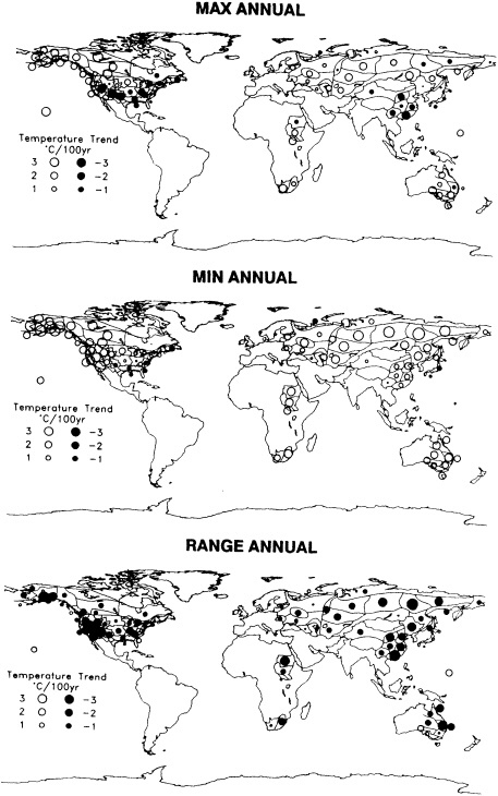
FIGURE 2
Spatial patterns of annual trends of mean maximum temperature, minimum temperature, and diurnal temperature range (mostly 1951-1990) in °C per 100 years. Diameter of circles is proportional to the trend; solid (open) circles represent negative (positive) trends. Circles pertain to regions within each country except for the island stations, e.g., the South Pacific and Hawaii.
TABLE 1 Trends of temperature (°C/100 years) for Annual and Three-Month Mean Maximum Temperature, Minimum Temperature, and Diurnal Temperature Range, Based on a Weighted Average of the Region (by country) in Figure 1.
|
Alaska 1951-1990 (39 stations) |
Japan 1951-1990 (66 stations) |
||||||
|
Seasons |
Max |
Min |
DTR |
Seasons |
Max |
Min |
DTR |
|
D-J-F |
6.0 |
8.8 |
-2.8 |
D-J-F |
-0.5 |
-0.2 |
-0.2 |
|
M-A-M |
3.1 |
6.3 |
-3.2 |
M-A-M |
-0.4 |
-0.7 |
0.3 |
|
J-J-A |
0.9 |
2.4* |
-1.5 |
J-J-A |
0.5 |
0.0 |
0.4 |
|
S-O-N |
-1.4 |
0.4 |
-1.9* |
S-O-N |
-0.3 |
-0.5 |
0.2 |
|
Annual |
2.1 |
4.5 |
-2.4 |
Annual |
-0.2* |
-0.4 |
0.2 |
|
Canada 1951-1990 (227 stations) |
People's Republic of China 1951-1988 (44 stations) |
||||||
|
Seasons |
Max |
Min |
DTR |
Seasons |
Max |
Min |
DTR |
|
D-J-F |
1.8 |
2.1 |
-0.2 |
D-J-F |
0.5 |
3.5 |
-3.0 |
|
M-A-M |
3.7 |
3.8 |
-0.1 |
M-A-M |
-0.8 |
1.4 |
-2.2 |
|
J-J-A |
0.5 |
1.4 |
-0.9 |
J-J-A |
-1.8 |
-0.8* |
-1.0 |
|
S-O-N |
-2.2 |
-1.2 |
-1.0 |
S-O-N |
-0.6 |
1.0 |
-1.6 |
|
Annual |
0.9 |
1.5 |
-0.6* |
Annual |
-0.7* |
1.3 |
-2.0* |
|
United States (contiguous) 1951-1990 (494 stations) |
South Africa 1951-1991 (12 stations) |
||||||
|
Seasons |
Max |
Min |
DTR |
Seasons |
Max |
Min |
DTR |
|
D-J-F |
-2.3 |
-0.7 |
-1.5 |
D-J-F |
0.8 |
2.0 |
-1.2 |
|
M-A-M |
2.3 |
2.5 |
-0.2 |
M-A-M |
2.2 |
1.7 |
0.5 |
|
J-J-A |
-0.3* |
1.0* |
-1.4 |
J-J-A |
1.3 |
1.3 |
0.0 |
|
S-O-N |
-1.7 |
1.3 |
-3.0 |
S-O-N |
-0.7 |
1.8 |
-2.4 |
|
Annual |
-0.6* |
1.0 |
-1.5 |
Annual |
0.9 |
1.7* |
-0.8* |
|
Sudan 1951-1987 (15 stations) |
Eastern Australia 1951-1991 (44 stations) |
||||||
|
Seasons |
Max |
Min |
DTR |
Seasons |
Max |
Min |
DTR |
|
D-J-F |
-1.2 |
2.7 |
-3.9* |
D-J-F |
1.8 |
2.3 |
-0.4 |
|
M-A-M |
0.4 |
3.3 |
-2.8 |
M-A-M |
1.6 |
2.8 |
-1.2 |
|
J-J-A |
2.8 |
2.1 |
0.7 |
J-J-A |
0.8 |
1.4 |
-0.5 |
|
S-O-N |
1.4 |
2.5 |
-1.1 |
S-O-N |
1.3 |
2.2 |
-0.9 |
|
Annual |
0.9 |
2.7 |
-1.7 |
Annual |
1.4 |
2.2 |
-0.7 |
|
USSR (former) 1951-1990 (165 stations) |
|||||||
|
|
|
Seasons |
Max |
Min |
DTR |
|
|
|
|
|
D-J-F |
2.8 |
4.2 |
-1.3 |
|
|
|
|
|
M-A-M |
2.5 |
3.8 |
-1.2 |
|
|
|
|
|
J-J-A |
-0.4* |
0.9* |
-1.3 |
|
|
|
|
|
S-O-N |
0.6 |
2.2 |
-1.6 |
|
|
|
|
|
Annual |
1.4 |
2.8 |
-1.4 |
|
|
|
Key: Trends significant at the .01 level (two-tailed t-test) are bold and italicized Trends significant at the .05 level are italicized Trends with significant change points are denoted with an asterisk |
|||||||
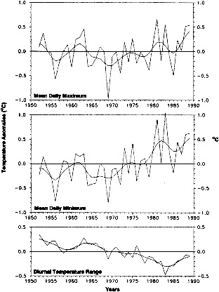
FIGURE 3
Time series of the temperature anomalies of the annual mean maximum temperature, minimum temperature, and diurnal temperature range for 37 percent of the global land mass (areas shaded in Figure 1). Smooth curve was obtained with a nine-point binomial filter with "padded" ends.
end of the time series is significantly affected by the drought. Furthermore, variance of the time series is significantly affected when such large regions drop out of the analysis, which is why the series ends prematurely. Nonetheless, Figure 3 reflects a gradual decrease of the DTR through much of the past several decades.
Longer-Term Variations
Unfortunately, the availability of maximum and minimum temperature data covering the globe is currently limited prior to 1951. In the United States a network of approximately 500 high-quality stations has remained intact since the turn of the century, and in the former Soviet Union a fixed network of 224 stations (165 if only rural stations are used) is available back to the 1930s. The time series from these two countries shown in Figure 4 reflect significant decadal variations in the DTR, which are particularly evident during the dry 1930s and the early 1950s in the United States. The general decrease of the DTR did not begin in the United States until the late 1950s, and the DTR decreased rather dramatically in the mid-to-late 1970s over the former Soviet Union as part of substantial increases in the minimum temperature. The decrease of the DTR in these two countries is a phenomenon of recent decades. Data are also available further back in time for smaller areas and countries, notably Japan, eastern Australia, and South Africa. Figure 5 indicates that the decrease in the DTR in eastern Australia has occurred rather gradually since the decline in the late 1940s. In South Africa the decrease is predominantly due to the sharp decline in the early 1950s.
A very long record of maximum and minimum temperatures was available from the Klementinum Observatory in Prague, Czech Republic, and another from a benchmark station from northern Finland. Figure 6 portrays a remarkable increase of the DTR at the Klementinum Observatory from the early twentieth to the mid-twentieth century, with a substantial decrease since about 1950. The increase coincides with the increase of global mean temperature since the turn of the century, and the decrease occurs when the
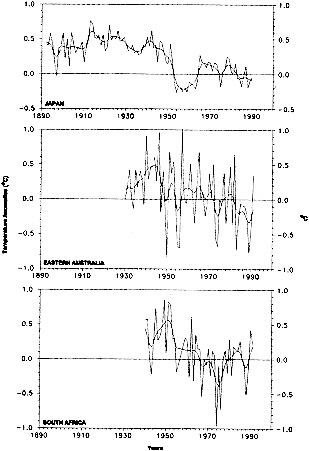
FIGURE 5
Time series of the variations of the diurnal temperature range for Japan, eastern Australia, and South Africa. Smooth curve was obtained with a nine-point binomial filter.
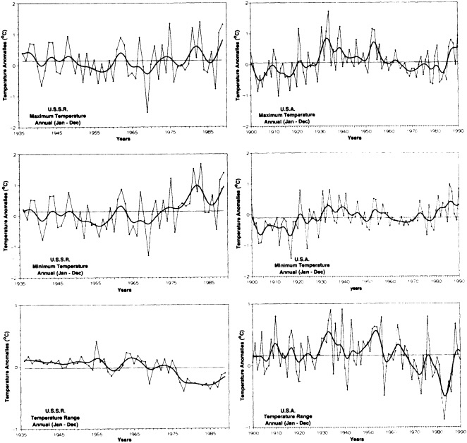
FIGURE 4
Time series of the variations of the annual mean maximum, minimum, and diurnal temperature range for the contiguous United States and the former Soviet Union. Smooth curve was obtained with a nine-point binomial filter. Trends since 1951 are depicted by the dashed line.
mean temperature reflects little overall change. In the first half of the nineteenth century the DTR averages about 0.5°C lower than in the latter part of the century. The DTR at Sodankylä, Finland, also displays a gradual decrease since 1950, but contrary to the Klementinum Observatory's pattern, the decrease is evident back to the turn of the century. The mean temperature at Sodankylä reflects little or no change. The high-frequency variability of the DTR at both stations is less than that of their respective mean temperatures, but the converse is true for low-frequency variations.
If the data from the Klementinum Observatory truly reflect the regional change of the DTR in central Europe, then the recent decrease of the DTR in this area is less persistent and less substantial than the increase prior to 1950. In light of the variations at the Klementinum Observatory, what makes the results from Figure 2 so remarkable
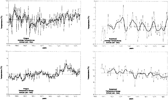
FIGURE 6
Time series of the variations of the annual mean temperature and the annual diurnal temperature range from two long-term stations: the Prague Klementinum-Observatory, Czechoslovakia, and Sodankylä, Finland, which has been designated as a climate reference station. Smooth curve was obtained with a nine-point binomial filter.
is the fact that so many areas share an overall decrease of the DTR.
Recently, other investigators have also compiled information on the change of the DTR over other portions of the globe. Frich (1992) provides evidence to indicate that there has been a general decrease over Denmark since about 1950, based on an analysis of several long-term stations, most located in rural areas. Bücher and Dessens (1991) analyzed a long record of maximum and minimum temperatures from the Pic du Midi de Bigorre Observatory in the Pyrenees at a height of over 2,800 m. Their analysis revealed a significant decrease of the DTR since the late nineteenth century, but an inhomogeneity in the record prevented a continuation of the analysis beyond 1970. Kruss et al. (1992) reported on changes of maximum and minimum temperature between the two 30-year periods 1931 to 1960 and 1961 to 1990 over Pakistan. Despite considerable missing data, they managed to obtain at least 20 years of data from each of the two periods for 35 stations across Pakistan. Their analysis revealed a mix of decreasing and increasing changes of the DTR. In our analysis of Pakistani data we could only manage to identify five stations with adequate data to analyze year-to-year changes, and these were all located in the northern half of the country. These stations also depicted a decrease of the DTR.
Relation to Variations of the Seasonal and Annual Extremes
For a variety of practical considerations, it is important to know whether the decrease in the mean DTR translates to a decrease in the extreme temperature range. Karl et al. (1991a) provide evidence to suggest that, indeed, over the United States and the former Soviet Union (the only areas for which they had access to daily data) there was often a significant and substantial decrease in the seasonal and annual temperature extremes similar to the decrease in the seasonal and annual mean DTR. This similarity is also reflected in the time series of monthly extreme maximum and minimum temperature over Sudan (Jones, 1992).
Data Quality
The reliability of the data used to calculate the changes of the DTR is a critical question. The data presented and discussed here have been subjected to various degrees of
quality assurance. The degree to which precautionary measures have been taken to minimize data inhomogeneities varies considerably from country to country. In the United States, a fixed network of stations in the Historical Climatology Network is used (Karl et al., 1990), which largely consists of rural stations that have been adjusted when necessary for random station relocations, changes in instrument heights, systematic changes in observing times (Karl and Quinn, 1986; Karl et al., 1986), the systematic change in instruments during the mid—and late 1980s (Quayle et al., 1991), and increases in urbanization (Karl et al., 1988). The potential warm bias of the maximum introduced by the H083 series of thermometer (Gall et al., 1992) is not a factor in this network, since the H083 instrument was not used in the rural cooperative network.
In the former Soviet Union, the fixed network of 165 stations consists of rural stations (1990 populations less than 10,000 and local surroundings free of urban development). The data from the former Soviet Union have not been adjusted for any random or systematic inhomogeneities. Station histories, however, indicate that there have not been systematic changes in that network's operation over the course of the past 50 years.
In Canada, the results reported here are derived from a set of 227 rural stations (those in areas with population less than 10,000). These data were selected from a network of 373 principal stations, but a large number of urban areas and stations that relocated to airports were eliminated from the analysis.
In Alaska, a network of 39 stations was used. It included most stations that had been operating in that state since the early 1950s, with the exception of the stations in the major cities of Juneau, Fairbanks, and Anchorage. Once again no attempt was made to adjust for station relocations, and the stations consist of a mix of instrument types with some changes at specific sites.
Station histories from China do not reflect any systematic changes in instrumentation, instrument heights, instrument shelters, or observing procedures relative to the maximum and minimum temperature. Our analysis is based on a subset of the more than 150 stations available to us. No attempt was made to correct for random station relocations in the fixed network of 44 stations we finally selected from the larger network. The potential impact of urbanization precluded the use of many stations; we eliminated all stations that were in or near cities with populations over 160,000.
All stations in Australia have recently undergone a thorough homogeneity analysis (Plummer et al., 1995), but the results were not available for this analysis. Instead, stations were selected on the bases of length of record and distance from major areas of urbanization. All of the Australian stations used are in small towns or rural areas, many in post office ''back yards."
Fewer than half of the 154 stations available from Japan were used in this analysis. As with China, many stations were eliminated because of their proximity to major urban areas. An inspection of the station histories reveals a number of network "improvements" related to the automation of the temperature measurements in recent years. A full assessment of the homogeneity of the data awaits a detailed analysis. The station networks from Sudan and South Africa include some stations from urban areas, but countrywide decreases of the DTR are not overwhelmed by these stations. Incomplete information was available regarding systematic changes in instrumentation at these locations over the past several decades, but the data were inspected for station relocations and adjustments made when necessary on the basis of temperature differences from neighboring stations. In total, four stations in South Africa were adjusted using the procedures outlined by Jones et al. (1986a).
INFLUENCES ON DIURNAL TEMPERATURE RANGE
Local Effects
As more data become available from a variety of countries, it becomes difficult to dismiss the general decrease of the DTR over the past several decades as an artifact of data inhomogeneities. Observing networks are managed differently in each country. If local effects are significantly influencing the DTR, then at least three possible sources of change need to be explored: urbanization, irrigation, and desertification. Evidence to support or refute the impact of these human-induced local and regional effects are discussed in the subsections below.
Urban Heat Islands
It is well known that the urban heat island often tends to manifest itself most strongly during the nighttime hours (Landsberg, 1981). In mid-latitude North American cities the urban-rural temperature difference usually peaks shortly after sunset, then slowly decreases until shortly after sunrise, when it rapidly decreases and, for some cities, actually vanishes by midday. In many cities increases in urbanization would differentially warm the minimum relative to the maximum temperature. A number of precautions have been taken to minimize this effect.
In the contiguous United States, the corrections for urban development recommended by Karl et al. (1988) have been applied to the data, and any residual heat-island effect in this analysis should not be an issue. In Canada, only stations with population less than 10,000 were used in the analysis, and the average population of the cities in the proximity of the observing stations was slightly over 1,000. If the Canadian stations behave similarly to stations in the United States, the effect on the diurnal temperature range may be
exaggerated by about 0.1°C. An effect of similar magnitude may exist for Alaska. In the former Soviet Union, the population limit for inclusion of any station into the network was 10,000; in addition, however, no station could be within 1 km of any multi-story urban development. If the impact of the effect of urbanization on the DTR in the former Soviet Union is anything like that in the United States, the residual urban heat island effect on the DTR should be at least an order of magnitude smaller than the observed decrease of the DTR (nearly 1.5°C/100 yr).
In China and Japan, a number of tests were conducted to identify the impact of urbanization on the DTR. Three networks of stations were categorized on the basis of population. For China the categories included stations in proximity to cities with populations over 1 million, under 160,000, and in between these two threshold values. Categories in Japan were based on threshold values of 500,000 and 50,000. In the three population categories, proceeding from high to low, China had 23, 42, and 44 stations while Japan had 17, 71, and 66 stations. Figure 7 shows that the decrease of the DTR actually is more marked in China for stations in the lowest population category than for stations in the medium category, while the trend of the average temperature continues to decrease. This unexpected finding suggests that urban-
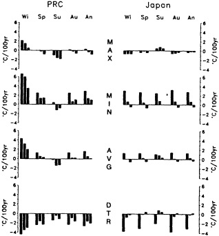
FIGURE 7
Temperature trends calculated for the People's Republic of China and Japan. Abbreviations: Wi, winter; Sp, spring; Su, summer; Au, autumn; MAX, maximum; MIN, minimum; AVG, average; and DTR, diurnal temperature range. The three bars in each of the seasonal and annual-average groupings reflect stations near cities in the high, medium, and low categories (left to right) as defined in the text.
ization effects in China are dissimilar to those in the United States, since they seem not to have affected the maximum and minimum temperature trends in Chinese cities of 500,000 or less. In Japan, however, the impact of urbanization on the DTR is evident even in the lowest population category (less than 50,000), and is even more apparent for the average temperature. On the basis of these analyses, it seems that the impacts of urbanization in China (Wang et al., 1990) are unlikely to significantly affect the trends reported in Tables 1 and 2.
A previous paper by Jones et al. (1990) investigated the impact of increasing urbanization in the land data base used by the IPCC (1990, 1992) to calculate changes of global temperature. The conclusion from the work of Jones et al. (1990) was that any residual urban bias in the land-based average temperature records was about 0.05°C during the twentieth century. A comparison of the average temperature trends derived from the stations used in Tables 1 and 2 with the stations used by Jones (1988) revealed differences in trends from country to country, but virtually identical trends of temperature (within 0.02°C/100 yr) were found when all areas depicted in Figure 1 were considered. This similarity suggests that the degrees of urban-induced bias in these two data sets are of comparable magnitude over the past 40 years, despite the use of substantially different station networks.
Irrigation
It can be argued that increases in irrigation may account for the decrease in the DTR. The evaporation associated with soil moisture would convert sensible to latent heat and thus significantly reduce daytime temperature. In order to test this hypothesis, the correlation coefficient (both the Pearson product-moment and the Spearman rank) was calculated using the values of the trends of the DTR and the change in land area under irrigation from 1950 to 1987 (U.S. Department of Commerce, 1950, 1988) for each of the regions in the United States delineated in Figure 2. No relationship was found between the change in the DTR and the increase of irrigated lands, and in fact many of the largest decreases of the DTR were associated with areas with the smallest increases of irrigation. Considering that the United States has had significant decreases of the DTR over the past several decades, and has had relatively large increases of irrigation relative to other countries over the past 40 years, it seems unlikely that increases of irrigation can be regarded as a serious explanation for the decreases of the DTR.
Desertification
The converse of the theoretical effects of irrigation would result from increased desertification. This might arise from
poor land practices such as over-grazing or deforestation. Given the mid- and high-latitude bias of the results reported here, it seems unlikely that desertification would have a significant impact on the results reported in Tables 1 and 2. Moreover, this effect would tend to make the reported decreases underestimates, especially during the warm season, as desertification would increase the maximum and decrease the minimum.
Climatic Effects
Since it seems unlikely that any of the human-induced local effects can provide a satisfactory answer to the widespread decrease of the DTR, a number of climatic variables that differentially affect the maximum and minimum temperature were analyzed to discern which of them most strongly affect the DTR. Over 50,000 days of climatic observations were selected from the stations listed in Table 3 during periods of consistent measurement procedures for the variables defined in Table 4.
The selection of variables to be studied was based on a priori information. For example, increases of the DTR over land have previously been related to snow cover ablation, in simulations by the U.K. Meteorological Office's general circulation model (GCM) with doubled CO2 (Cao et al., 1992). It is well known that the ability of the surface boundary layer to absorb, radiate, transform, and mix sensible heat differentially affects the maximum and minimum temperature. Relative humidity and cloudiness are two important climate variables that influence these surface-layer properties. In this analysis cloud-related information was contained in two climatic variables, the sky cover (in tenths) and an index of the ceiling height. The ceiling height (CIG)
TABLE 3 Stations and Years Used in Identifying the Sensitivity of the Diurnal Temperature Range to Various Climatic Variables
|
Stations |
Years |
|
Sacramento, CA |
1961-69 |
|
Tallahassee, FL |
1962-70 |
|
Indianapolis, IN |
1966-74 |
|
Worcester, MA |
1961-69 |
|
Bismarck, ND |
1973-81 |
|
Scotts Bluff, NE |
1971-79 |
|
Reno, NV |
1961-69 |
|
Oklahoma City, OK |
1975-83 |
|
Pittsburgh, PA |
1961-69 |
|
Columbia, SC |
1971-79 |
|
San Antonio, TX |
1973-81 |
|
Seattle/Takoma, WA |
1971-79 |
|
Spokane, WA |
1966-75 |
|
Green Bay, WI |
1971-79 |
TABLE 4 Definitions and Abbreviations of the Climatic Variables Used to Test the Sensitivity of the Diurnal Temperature Range
|
Variables |
Abbreviations |
|
Diurnal temperature range (daily max-daily min) |
DTR |
|
Snow cover (binary, if snow depth ≥2.54 cm) |
SNOW |
|
Mean relative humidity (0600 LST* & 1500 LST) |
RH |
|
Mean wind speed (0600 LST & 1500 LST) |
WS |
|
Mean sky cover (0600 LST & 1500 LST) |
SKY |
|
Mean ceiling (0600 LST & 1500 LST) |
CIG |
|
Total daily top-of-the-atmosphere solar radiation |
TRAD |
|
Day-to-day temperature differences |
ΔTMP |
|
(|TMP0 − TMP−1 | + |TMP0 − TMP+1|) |
|
|
* local standard time |
|
was broken down into seven categories. The cloud ceiling is defined as height above ground of the lowest cloud layer that covers 50 percent or more of the sky. The wind speed is an effective measure of the degree of mixing within the surface boundary layer, since it affects and interacts with the frequency and/or intensity of inversions and superadiabatic lapse rates.
In addition, the DTR is affected by the seasonal and latitudinal changes of incoming solar radiation as well as by the magnitude of day-to-day temperature differences. TRAD (top-of-the-atmosphere solar radiation) can also be regarded as a surrogate for the temperature, especially when it is used in conjunction with the other variables listed in Table 4. Karl et al. (1986) demonstrate the impact of the interdiurnal temperature difference on the maximum and minimum temperature. Large interdiurnal temperature differences lead to a large temperature range, even in the absence of a diurnal temperature cycle. These day-to-day changes of temperature are largely controlled by the thermal advection associated with synoptic-scale cyclones and anticyclones.
All of the variables in Table 4 were used in a multiple-regression analysis. Variables were regressed against the square root of the DTR, as opposed to the actual DTR, because the DTR is bounded by zero. Without the transformation, non-normal residuals result in multiple linear-regression analyses, making it more difficult to interpret the results. Figure 8a indicates that the partial-correlation coefficients of each variable with respect to the DTR are often significantly different from the simple linear correlation coefficients, making it difficult to speculate on the effect of changes in any one variable without knowing the changes in (or assuming constancy of) the other variables. Given the huge sample size, very low correlations have high statistical significance (even considering the day-today persistence of the DTR). On a local basis, a generalized
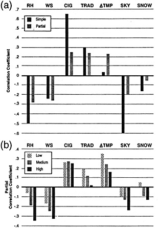
FIGURE 8
Relationship between various climate variables and the diurnal temperature range. (a) Simple and partial correlation coefficients (removing the effects of all other variables) between each variable (defined in Table 4) and the diurnal temperature range. (b) Partial correlation coefficients of each variable for cases partitioned by the total daily solar radiation at the top of the atmosphere: 170 W m−2 (low), ≥271 W m−2 (high), and remainder (medium).
multiple linear-regression model (one model for all stations and all days) based on the seven climatic variables in Figure 8a explains about 55 percent (53 percent without the square-root transformation) of the daily variance of the DTR. Although the explained variance is substantial, it is apparent that other factors may also need to be considered in order to explain the variations of the DTR (e.g., better representations of the atmospheric stability, external forcing factors, more precise techniques for calculating the mean quantities used in the analysis) and their relationships are not adequately expressed by a linear equation.
On a variable-by-variable basis, the signs of all the partial correlations make qualitative physical sense. It is interesting to note that the partial correlation of ΔTMP with DTR is greater than that of the simple correlation coefficient (Figure 8a), because the correlation between TRAD and ΔTMP mask the importance of ΔTMP in influencing DTR. The decrease of the partial correlation relative to the simple correlation for the variables RH, CIG, and SKY is to be expected, because changes among these variables are all related to each other. The decrease in the partial correlation of SNOW is particularly noteworthy, especially since Cao et al. (1992) attribute the ablation of snow cover in their model to an increase in the DTR. The empirical results in Figure 8a suggest that SNOW is only weakly related to DTR (7.5 percent of the cases, nearly 4,000, had snow cover), especially by comparison with the other variables.
In order to investigate the linearity, or lack thereof, of the relationships implicit in Figure 8a, the data were partitioned by TRAD. Figure 8b provides strong evidence to suggest that the relationships change with the amount of TRAD. In particular, the partial correlation coefficients of RH, WS, and SKY become stronger as TRAD (and thus temperature) increases. This probably has more to do with a reduction of the maximum temperature than an increase of the minimum. During daylight hours high values of the RH, WS, and SKY are indicative of higher albedos, higher potential evapotranspiration, higher atmospheric water-vapor absorption of incoming radiation, and larger-than-normal mechanical mixing. These factors act to reduce the maximum temperature that would otherwise result from high-intensity TRAD, which would be manifested as sensible heat within the surface boundary layer. The non-linearity of RH as TRAD increases is substantially greater than that of WS (Figure 8b). As the TRAD reaching the surface increases, the temperature increases, and comparatively more of the TRAD can be used for evaporation than for raising surface temperature, as would be anticipated by integrating the Clausius-Clapeyron equation to obtain saturation vapor pressure as a function of temperature.
The reduction of the partial correlation of TRAD with the DTR when the sample is partitioned with respect to TRAD (Figure 8b) relates to the balance between long nights and short days. During the late autumn and early winter in the northern half of the United States (areas which include the lowest partition of TRAD), a moderate increase in the TRAD (by inter-seasonal and latitudinal variations) generally results in a higher DTR. Contrarily, in the warm half of the year, TRAD is more than ample, so the relation between TRAD and DTR is near zero. In fact, a further selection for very high values of TRAD (short nights) leads to small negative partial correlations between TRAD and the DTR.
The reduction of the partial correlation of ΔTMP as TRAD increases is related to the decrease in intensity of the day-to-day changes of temperature during the warm season. Rossby waves and extra-tropical cyclones have lower amplitude, speed, and intensity during the warm season.
A change in sign of the partial correlation coefficient of
SNOW with the DTR (Figure 8b) suggests that the length of night relative to the TRAD is a significant factor in the impact of changes of snow cover on the DTR. In the northern United States, around the winter solstice, TRAD is relatively low. Snow on the ground at this time of year is important because of its excellent insulating properties (it reduces heat flow from the soil), which help lower the nighttime minimum. During the daytime the TRAD is already low, so the amount of solar radiation reflected by the snow cover is no longer so important. As a result, snow cover at this time of year at these latitudes leads to an increase in the DTR. This is not the case as the season progresses or the latitude decreases, as is reflected by the negative partial correlations (lower values of DTR with snow cover) associated with the highest category of TRAD, where there were still nearly 1,000 cases of snow cover. The data suggest that snow-cover ablation will not necessarily lead to an increase of the DTR.
From the above analysis it is apparent that there are many factors, often intricately related, that affect the DTR. Many of these variables are very much related to a greenhouse effect, not necessarily one anthropogenically induced. Overall, however, the two variables related to changes in cloudiness, sky cover, and ceiling height explain the greatest portion of the variance of the DTR. Changes in cloudiness should be one of the first considerations in searching for an explanation of the observed decrease of the DTR (Figure 2). Indeed, when large continental scales are considered, the relationship between cloud amount (or sky cover) with the DTR is quite impressive (Figure 9). Plantico et al. (1990) have already demonstrated that the decrease in the DTR
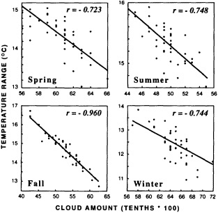
FIGURE 9
Seasonal relationships between U.S. area-average cloud cover and the diurnal temperature range.
over the United States is strongly linked to an observed increase in daytime and nighttime cloud cover and to a lowering of cloud ceilings.
Is there a general increase in cloud cover over much of the globe? Empirical evidence by Henderson-Sellers (1986, 1989, 1992) and Jones and Henderson-Sellers (1992) suggests that this may be the case over Canada, the United States, Europe, the Indian subcontinent, and Australia. Analyses of cloud cover changes over China from a network of 58 stations are inconclusive, but there is evidence for a decrease in the sunshine (a 2 to 3 percent decrease in sunshine from the 1950s to the 1980s). The quality of the cloud data (and perhaps the sunshine data) is questionable because the correlation between monthly anomalies of sunshine and cloudiness at many sites is not high. Analyses of changes in cloudiness over the former Soviet Union by Kaiser and Razuvayev (1995) reveal a general increase of cloud cover (about 5 percent) over the period 1936 to 1986, with cirrus increasing in frequency by nearly 20 percent. They also found considerable interannual and interstation variability, so the quality of these data could also be called into question. Nonetheless, the trend over the former Soviet Union is consistent with a decrease in the DTR. Frich (1992) and Bücher and Dessens (1991) also found that decreases in the DTR in Denmark and at the Pic du Midi de Bigorre Observatory occurred concurrently with an increase in cloudiness. An analysis of changes in cloud cover over Japan, using many of the same stations selected for the analysis of the maximum and minimum temperatures, indicates that cloud cover may have increased on an annual basis by nearly 1 percent since 1951, but there is no apparent response in the DTR. Changes in sunshine in Japan are not altogether consistent with the increase in cloud cover, perhaps because a new instrument was introduced into the network in 1986.
LARGE-SCALE ANTHROPOGENIC EFFECTS
Greenhouse Gases
Interest in the possible change of the DTR with increasing anthropogenic greenhouse gases has prompted several modeling groups to publish information from their models regarding the change in projected DTR when CO2 is doubled. Table 5 summarizes the results of these models. For the GCM experiments, the magnitude of the decrease in DTR is small relative to the overall increase of mean global temperature. Moreover, these experiments reflect a level of CO2 increase well in excess of present-day values, so even smaller changes would be expected in the observed-temperature record. Outside of the Rind et al. (1989) study, only Cao et al. (1992) focus specifically on the changes of the DTR over land areas. Cao et al. show that their model can reasonably simulate the range of the present-day diurnal
TABLE 5 Summary of Modeling Results Showing the Relationship Between Doubled CO2 Concentrations and Changes in the Diurnal Temperature Range and the Maximum and Minimum Temperatures
|
General-Circulation Models |
||||||
|
|
|
Resolution |
||||
|
Model |
Author |
Horizontal |
Vertical |
Ocean |
ΔTeq |
ΔDTReq |
|
CCC |
Boer (pers. comm.) |
T32 |
10 |
Mixed layer |
3.5 |
−0.28 |
|
GISS |
Rind et al. (1989) |
8° × 10° |
9 |
Mixed layer |
4.2 |
−0.7 |
|
|
|
|
|
|
|
(summer, USA) |
|
|
|
|
|
|
|
−0.1 |
|
|
|
|
|
|
|
(annual, USA) |
|
UKMO |
Cao et al. (1992) |
8° × 10° |
11 |
Mixed layer |
5.2 |
−0.17 |
|
UKMO |
Cao et al. (1992) |
5° × 7.5° |
11 |
Mixed layer |
6.3 |
−0.26 |
|
Radiative Convective Model (Cao et al., 1992) |
||||||
|
Type |
|
ΔMaximum Teq |
|
ΔMinimum Teq |
|
ΔDTReq |
|
Fixed absolute humidity |
|
N/A |
|
N/A |
|
−0.05 |
|
No surface turbulence |
|
2.5 |
|
2.9 |
|
−0.4 |
|
No evaporation |
|
2.3 |
|
2.9 |
|
−0.6 |
|
Full surface exchange |
|
1.5 |
|
2.2 |
|
−0.7 |
|
Key: ΔTeq is the equilibrium global temperature change (°C) for doubled CO2 concentrations ΔDTReq is the equilibrium global change of the DTR (°C) for doubled CO2 concentrations CCC is the Canadian Climate Centre GISS is the Goddard Institute for Space Studies UKMO is the U.K. Meteorological Office |
||||||
temperature cycle, although the modeled diurnal range in mid-latitudes is generally less than the observed.
Cao et al. (1992) also conducted a number of experiments with a one-dimensional radiative-convective model (RCM) to show that the decrease in the diurnal temperature range with doubled CO2 in that model is due primarily to a water-vapor feedback. A reduction of only 0.05°C in the DTR was observed when the absolute humidity was held constant. Table 5 indicates that increased sensible-heat exchange and evaporation are also important factors leading to a reduction in the DTR in RCM simulations with enhanced CO2.
Interestingly, the ratio of the DTR decrease relative to the increase of the mean temperature is closer in the RCM to the observed ratio over the past several decades than it is in the GCM (Table 5). The RCM omits the positive feedbacks to the DTR from reductions in cloud and surface albedo included in the GCM simulations (Cao et al., 1992). These feedbacks tend to increase the DTR because of reduced atmospheric (cloud cover) and surface (snow cover) albedo. Other GCMs simulate both increases and decreases in cloudiness from global warming—decreases in much of the troposphere, but increases in the high troposphere, low stratosphere, and near the surface in high latitudes (Schlesinger and Mitchell, 1985). A tendency for a general increase in cloud cover over land (which now seems likely from the observational evidence) could help explain the large discrepancy between the observed data and the model projections of the ratios of the decrease in the DTR range relative to the mean temperature increase. (This explanation assumes, of course, that the recent warming is induced by increases in anthropogenic greenhouse gases. On the other hand, it leaves questions regarding the cause of the apparent change in cloudiness and how it has affected the mean temperature.)
The ability of present-day GCMs to adequately simulate changes in the DTR resulting from enhanced CO2 is also affected by surface parameterizations of continental-scale evaporation. As Milly (1992) points out, present-day GCMs can overestimate the surface evaporation because of their failure to properly account for the cooling that occurs with the evaporation. Milly raises concerns about the veracity of the results from studies of soil-moisture changes induced by an increase of greenhouse gases. Accurate projections of the changes in the surface boundary-layer DTR with increases of anthropogenic greenhouse gases will be strongly dependent on adequate simulation of these processes.
Given the dependency of the DTR on surface-layer processes, interactions with the land surface, and cloudiness (which are all areas of significant uncertainties within pres-
ent-day GCMs), it may not yet be possible to adequately project changes of the DTR with enhanced concentrations of greenhouse gases.
Tropospheric Aerosols
It has recently been shown that increases in sulfate aerosols over and near industrial regions can have a significant impact on the earth's surface temperature (Charlson et al., 1992). Charlson et al. (1991, 1992) provide evidence to indicate that the anthropogenic increase of sulfate (and carbonaceous) aerosol is of sufficient magnitude to compete regionally with present-day anthropogenic greenhouse forcings. This forcing, which is confined primarily to the Northern Hemisphere, is a combination of direct aerosol forcing (especially over land) and indirect aerosol forcing leading to increases in cloud albedo (especially over the marine environment). Charlson et al. (1992) conclude that at present not enough is known to allow the effects of sulfate aerosols on the lifetime of clouds to be estimated. Increased aerosols (cloud condensation nuclei) could lead to smaller droplet sizes, causing a decrease in the fallout rate, which in turn could lead to an increase in cloud cover. Charlson et al. (1991) show a pattern of the geographic regions where direct aerosol forcing should be greatest. It is difficult to identify a direct relation between the pattern and magnitude of the decrease in the DTR (Figure 2) and the anthropogenic radiative forcing (Charlson et al., 1991). For example, on an annual basis over the United States the clear-sky daytime forcing varies from essentially zero (over several western states) to about -4 W m-2 (over southeastern states). It also varies with season by roughly a factor of 2 to 3, being greatest during summer.
Recently Penner et al. (1992) have argued that atmospheric aerosols from biomass burning also act to increase the planetary albedo, both directly by clear-sky planetary albedo increases and indirectly through increases in cloud albedo. Since biomass burning is most extensive in subtropical and tropical areas, this effect may be directly relevant to only a small portion of the data analyzed here.
Two tropospheric-aerosol forcings that tend to increase the clear-sky albedo have been identified. Has either of these forcings acted to reduce the maximum temperature and thereby the DTR? In the United States and northern (and perhaps eastern) Europe, where we detected a significant decrease in the DTR, there has actually been a net decrease in sulfur emissions over the past several decades, which would appear to eliminate sulfate aerosols as a cause of the DTR in these areas. However, there are reasons why such a conclusion may be premature. First, there is considerable geographic, seasonal, and secular variation of anthropogenic sulfur emissions. For example, Figure 10 shows the emissions of SO2 gas (precursor of the sulfate aerosol) doubling over the southeastern United States from 1950 to ca. 1980,
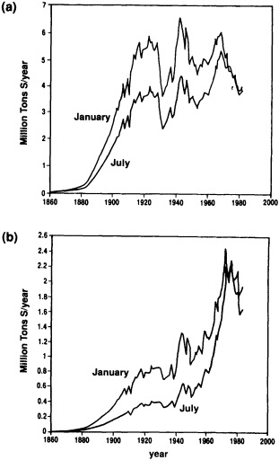
FIGURE 10
Time-dependent emissions of SO2 gas for (a) the northeastern United States and (b) the southeastern United States.
and then decreasing by 25 percent since then, while emissions have remained nearly constant in the northeastern United States. Also, the direct climate forcing due to tropospheric aerosol loading is influenced by (1) the absence of cloud cover, (2) the emission rate, and (3) the residence times of sulfate aerosol in the atmosphere, which are known to be short (about a week, according to Slinn (1983)). Second, in the United States at least, the effective heights, or stack heights, of the sulfur emissions have increased as a consequence of rural electrification in the southeast and, later, of the U.S. Clean Air Act. This increase in stack height may have had an important effect on the lifetime of SO2 and the sulfate aerosols (because of their relatively short lifetimes) and, consequently, on the aerosol concentration. Third, the indirect effects of sulfate aerosols on the DTR must also be considered, e.g., more cloud cover or a changing distribution of cloud characteristics.
CONCLUSIONS
Strong evidence exists for a widespread decrease in the DTR over the past several decades in many portions of the globe. The climatic factors that can affect the DTR are many, but indications are that cloud cover, including low clouds, has increased in many areas where DTR has decreased. These increases in cloud cover could be indirectly related to the observed global warming and increases of greenhouse gases (or perhaps even to the indirect effects of increases in aerosols), could be simply a manifestation of natural climate variability, or could reflect a combination of all three.
Obtaining a robust answer regarding the cause(s) of the decrease in the DTR will require efforts in several areas. First, an organized global effort is needed to develop relevant and homogeneous time series of maximum and minimum temperature, along with information on changes of climatic variables that influence the DTR, such as cloudiness, stability, humidity, thermal advection, and snow cover. Second, improvements in the boundary-layer physics and treatment of clouds within existing GCMs is critically important. Third, the treatment of both anthropic tropospheric aerosols and greenhouse gases must be realistically incorporated into GCMs with a diurnal cycle. Fourth, measurements need to be made to help clarify the role of aerosols. These include (1) data on diurnal, seasonal, and geographic changes in solar radiation, in areas influenced by aerosol forcing and areas free of it; (2) simultaneous data on key aerosol properties (mass-scattering efficiency, wavelength dependence, backscatter fraction/asymmetry factor), concentration, and composition; (3) data related to changes in all the relevant cloud parameters and their coupling to aerosol changes (if any); and (4) improved chemical models to allow more accurate calculation of the sulfate aerosol effects and to provide an estimate of the time course of this aerosol forcing. Finally, imaginative climate-change detection studies that link the observed climate variations to model projections will be required to convincingly support any relationship between anthropogenic changes and the DTR.
It will be difficult to satisfactorily explain the observed changes of the mean temperature until an adequate explanation for the observed decrease in the DTR can be determined. Moreover, the practical implications of projected temperature changes and whether they are likely to continue will be even more difficult to assess.
ACKNOWLEDGMENTS
This work was supported by a U.S. Department of Energy/National Oceanic and Atmospheric Administration (NOAA) interagency agreement and NOAA's Climate and Global Change Program.
We thank the following scientists for providing us with additional data: Reino Heino for the Sodankylä data, and Takehiko Mikami for the Japanese data.
Discussion
GOODRICH: Tom, were you able to use the ISCCP data sets to test your hypothesis that the decrease in the annual range of cloudiness might be associated with temperature?
KARL: I think there might be problems with both the longevity and the quality of those data, and the solar radiation data network is not as comprehensive as one might wish. We really need to get cloud and temperature experts together to see whether relating the two makes sense.
CHARLSON: To determine how cloud cover affects heat balance you would really need to know cloud liquid-water content and mean droplet size, as well as cloud area. All three govern the system albedo. The ISCCP data don't have those, and I'm not sure our current remote-sensing systems have that capability either. If we found a correlation, we wouldn't know whether it was caused by cloud microphysics or dynamics.
SHUKLA: Tom, one of your most dramatic differences was that between the rural and urban areas of Japan. Would it be naive to ask whether radiative forcing associated with urban pollution could be involved?
CHARLSON: Urban haze around most cities actually extends for hundreds of kilometers. Also, neither the soot aerosols nor the light-absorbing gases in smog cause any great amount of heating.
KARL: Various studies have shown that maximum temperature is not much affected by urbanization. But it is a significant point to keep in mind, especially given how it dominates the record in Japan.
KEELING: Many of you have probably heard of the Arctic and Antarctic borehole data that suggest that the heat flux from the interior of the earth is not steady state. Is it possible that these borehole temperatures are showing the effects of nighttime radiative warming?
CHARLSON: The next set of NCAR model calculations will be simulating diurnal temperature range, and a model in Hamburg is doing that too. It will be interesting to hear their results.
RIND: Our GCM looked at diurnal temperature change for doubled CO2 . We found that for a 4° warming we got about a 10 percent change, or 1°C. That was primarily during the summer, so we did not get the one-to-one correspondence you see in the data. I also wanted to mention that the ISCCP data set can't get optical thicknesses for nighttime clouds, since they can't measure the albedos.
KARL: I should perhaps add that while most of the CO2-doubling models show a decrease in diurnal temperature range of maybe 10 percent of the equilibrium temperature, the simple radiative convective model of Cao et al. shows fairly large decreases. I really think that there's some question whether a GCM can be expected to reproduce the diurnal cycle, given the type of land-surface physics involved.
Decadal Oscillations in Global Temperature and Atmospheric Carbon Dioxide
CHARLES D. KEELING AND TIMOTHY P. WHORF1
ABSTRACT
Since 1958, global air temperature has been found to correlate with the concentration of atmospheric CO2 on interannual time scales, from biennial to decadal. The decadal variations also correlate approximately with the 11-year sunspot cycle. Although CO2 data are lacking before 1958, global temperature data are available back to the 1850s. No consistent solar correlation is evident in this longer record. Instead, the record shows a decadal pattern that can be expressed by two oscillations having periods of approximately 9 and 10 years. These oscillations show reinforcement in the 1880s and 1970s and interference in the 1920s. Thus, decadal oscillations appear to have been relatively prominent in the latter half of the nineteenth and twentieth centuries, while being weak or absent from about 1905 to 1940. In the absence of an identified mechanism that would explain this pattern, the results must be treated as tentative.
INTRODUCTION
Several years ago we detected a possibly cyclic variation in the concentration of atmospheric CO2 (Keeling et al., 1989). The period of variation, of the order of 10 years, appeared to be synchronous with a decadal oscillation in air temperature when both records were band-passed to remove high- and low-frequency fluctuations and the influence of fossil-fuel combustion on the CO2 concentration. As shown in the upper panel of Figure 1, the adjusted 32-year CO2 record shows maximum concentrations near 1961, 1971, and 1981, the same years in which decadal maxima in air temperature occur. The maxima in CO2, especially the latter two, nearly coincide with maxima in the number of sunspots (lower panel) as though both CO2 and temperature were influenced by changes in solar irradiance. The investigation was not extended back to early times, because of a lack of CO2 data.
Globally averaged surface air temperature anomalies have been determined back to 1854, however (Jones and Wigley, 1991). To extend our analysis, we have accordingly computed the difference between two smoothing splines fit to this temperature record, where the differing stiffnesses of the splines result in band-passed data similar to those shown in Figure 1. The results, plotted in Figure 2 together with the record of sunspots, suggest that the positive correlation of global temperature with sunspot numbers is transi-
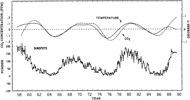
FIGURE 1
Decadal variability of anomalies in global averaged atmospheric CO2 concentration (in parts per million by volume (ppm)) and in global surface temperature (in °C) compared with decadal variations in sunspot numbers, modified from Keeling et al. (1989, Figure 66). Upper curves: Approximately 10-year oscillations in atmospheric CO2 concentration (dashed curve) and global temperature (solid curve), calculated as differences between splines of different stiffness. For CO2 the stiffer spline has a standard error (s of 0.245 ppm with respect to monthly averaged data (1958-1989); the less stiff spline has an error of 0.200 ppm. For temperature over the same time period the stiffer spline has a s of 0.088°C. Lower curve: Sunspot numbers (National Geophysical Data Center, 1989), shown as line segments connecting monthly averages. The CO2 record in 1968 and 1969 was modified from that reported by Keeling et al. (1989) as a result of a reassessment of the original calibrating data.
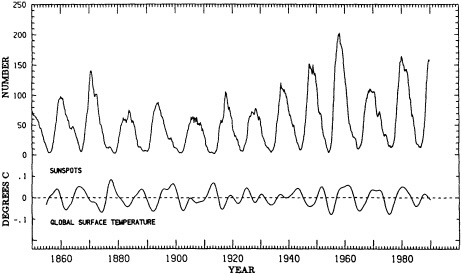
FIGURE 2
Comparison of a 12-month running mean of sunspot numbers (upper curve) with a decadal band-pass filter of global surface temperature in °C (lower curve). The latter is the same as that shown below in panel 2 of Figure 4.

FIGURE 3
Global surface temperature anomaly from 1855 through 1989, in °C (Jones et al., 1986c, and Jones, private communication). Monthly data are shown as dots. The solid curve is a spline fit through this monthly data with a s of 0. 10°C.
tory. The two decadal-scale peaks immediately prior to 1961 (in 1943 and 1952) came well after the sunspot maxima of 1938 and 1948; a series of decadal oscillations appeared before 1905, but the peak temperatures occurred near times of minimum sunspots, rather than near maxima. From about 1905 to 1940, instead of decadal oscillations, the temperature record shows oscillations with periods of only about 6 years.
Although these 6-year and decadal variations may reflect internal oscillations of the coupled atmospheric-oceanic circulation system (James and James, 1989), or simply a noisy record that falsely appears to be periodic from time to time (Gribbin, 1979), the present evidence does not, in our view, conclusively rule out the possibility of a persistent decadal periodicity in temperature. It is our purpose here to describe this possible decadal signal to help decide whether its recent appearance, where it correlates with atmospheric CO2, is short-lived, or whether instead it might reflect an oscillatory feature of the long-term temperature record, present in spite of the lack of evidence for a simple mechanism (such as solar forcing) that could produce it.
ANALYSIS OF OSCILLATIONS IN AIR TEMPERATURE
To investigate decadal-scale variations in temperature we have made use of a compilation of monthly averaged Northern and Southern Hemisphere temperature anomalies both over land and in surface seawater, originally summarized by Jones et al. (1986c) but later supplemented by additional data for the years 1854-1860 and 1985-1989, inclusive. The globally averaged data that we used directly in our computations are listed in Appendix A below.
The large scatter in monthly averaged global temperature data (the dots plotted in Figure 3) is not a strong encouragement to look for cyclic phenomena. Nevertheless, if the data are fit to a flexible smoothing spline (Reinsch, 1967) to suppress the high-frequency scatter (the solid curve in Figure 3), persistent periods of warmer and cooler conditions show in the record. The average spacing of warming and cooling events is between 3 and 4 years, depending on how many of the minor fluctuations are considered significant. A large number of the warmer periods occurred close to the times of El Niño events. It seems likely that the latter reflect phenomena that originate mainly in the Indo-Pacific region of the tropics (Quinn et al., 1987; Quinn and Neal, 1992) as a result of interactions of the atmosphere and oceans that arise from imbalances in the coupled system unrelated to any possible external forcing. If only the stronger warm events are counted, the recurrence interval becomes about 9 years (Quinn and Neal, 1992), so that El Niño events cannot be ignored in considering the possible causes of decadal variations in temperature. However, if they are so related, one would not expect them to be closely periodic.
To obtain a closer look at possible decadal-scale fluctua-
tions in temperature, we have fit the individual data points of Figure 3 to three additional smoothing splines of successively greater stiffness (Figure 4, panel 1), chosen to produce increasing degrees of low-pass filtering of the monthly data (Enting, 1987). The choices were subjective, but are not critical to the outcome, because distinct decadal patterns can be produced over a considerable range of stiffnesses. These three spline fits were run on both monthly and yearly averaged data, and the resulting curves showed essentially no difference. The stiffest spline (the curve labeled ''1") shows only a tendency for global air temperature to rise irregularly since 1855. The two looser splines (curves "2" and "3"), whose difference is shown in panel 2, are nearly identical to the spline curves whose difference produced the approximately decadal band-pass of temperature that is shown in Figure 1. The difference between curves " 1" and "2" (Figure 4, panel 3) approximates a band-pass centered near 20 years, while the difference between curves "1 " and "3" (Figure 4, panel 4) approximates a broader band-pass showing temperature fluctuations on both decadal and bidecadal time scales.
To examine further the spectral character of the global temperature record of Jones and co-workers, we have computed a series of spectra of their record by the maximum entropy method (MEM) (Press et al., 1989). This method of spectral analysis includes both the Thomson multitaper method and the fast fourier transform (FFT) method. Its results are particularly suitable for trying to resolve closely spaced frequencies (Press et al., 1989; Berger et al., 1990). We afterwards established the amplitudes and phases of the identified spectral peaks by least-squares fits of sinusoidal functions, since the maximum entropy method, as discussed by Sonett (1983), is not quantitatively reliable with respect to amplitudes and cannot establish phase relationships.
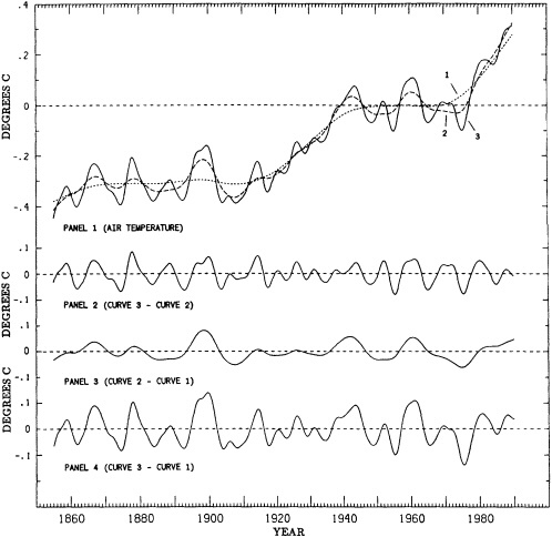
FIGURE 4
Global temperature anomaly from 1855 through 1989, based on annual averages of the data in Figure 3 (Use of monthly data showed negligible difference at these decadal frequencies.) Panel 1: Three superimposed spline fits. The dotted curve "1" is a very stiff spline (s equal to 0.106°C); the dashed curve "2" and solid curve "3" are looser spline curves (s's of 0.095°C and 0.075°C). Panel 2: Curve "3" minus curve "2". Panel 3: Curve "2" minus curve "1". Panel 4: Curve "3" minus curve "1".
Specifically, we first carried out an MEM analysis of the original monthly "raw" data (shown as dots in Figure 3), with only a linear trend subtracted. The data set consisted of 1620 points. Spectral estimates were obtained for order M (number of poles; see Press et al. (1989)) equal to 750. The periods of the 24 most prominent spectral peaks found are listed in the first column of Table 1 for frequencies greater than 0.6 cycles per year. Since the use of such a large number of poles invites criticism that we have exceeded the limits of the MEM method, we carried out a second analysis in which we first removed the lowest and highest frequencies from the record by subtracting the very stiff curve "1" shown in Figure 4 from the flexible spline shown in Figure 3. The resulting detrended and slightly smoothed temperature record is shown in Figure 5, panel 1. It can be seen by comparison with Figure 3 that almost all of the oscillatory character in the original record with periods between 1 and 30 years is retained in panel 1 of Figure 5. We then calculated the MEM spectrum on the basis of this slightly
TABLE 1 MEM Spectra of Monthly Global Surface Temperature, 1855-1989
|
Raw Data Spectrum* (years) |
Smoothed (years) |
Amplitude for 24-Harmonic Fit** (°C) |
Non-parametric Multitaper (years) |
|
41.3 |
31.40 |
0.017 |
|
|
22.10 |
21.69 |
0.039 |
20.5 |
|
15.28 |
15.59 |
0.038 |
15.5 |
|
10.07 |
12.15 |
0.017 |
|
|
9.18 |
10.22 |
0.036 |
|
|
7.509 |
9.29 |
0.037 |
9.1 |
|
6.643 |
7.610 |
0.014 |
|
|
6.042 |
6.670 |
0.026 |
|
|
5.218 |
6.043 |
0.037 |
6.1 |
|
4.740 |
5.227 |
0.040 |
5.2 |
|
4.382 |
4.758 |
0.041 |
4.8 |
|
4.128 |
4.436 |
0.023 |
|
|
3.756 |
4.170 |
0.026 |
4.0 |
|
3.546 |
3.746 |
0.022 |
3.8 |
|
3.283 |
3.548 |
0.034 |
3.5 |
|
3.122 |
3.290 |
0.025 |
|
|
2.867 |
3.127 |
0.022 |
|
|
2.716 |
2.866 |
0.027 |
|
|
2.318 |
2.727 |
0.009 |
|
|
2.241 |
2.320 |
0.023 |
|
|
1.998 |
2.242 |
0.017 |
|
|
1.885 |
1.997 |
0.020 |
|
|
1.796 |
1.884 |
0.014 |
|
|
|
1.797 |
0.017 |
|
|
* From Ghil and Vautard (1991, Figure 2). Their plot also shows an unlabeled, strong peak near 10.2 years. ** From a fit of sine and cosine functions to the smoothed data. The amplitudes are peak to trough. |
|||
smoothed record with data points spaced three months apart, beginning with January 1855. The data set consisted of 540 points. Given the degree of smoothing of this record, more closely spaced data would not have contributed any significant additional information, as perhaps they could have done if the raw data had been used. As shown in the second column of Table 1, the power spectrum of the slightly smoothed record, with M set equal to only 250, gives almost the same frequencies for peaks as the spectrum based on the raw data with M set equal to 750.
A check was also made by creating a subset of points, reducing the raw data by a factor of 3 (selecting values for every third month only, beginning with the first). With a linear trend removed as before, we obtained nearly the same spectrum with M set equal to 275 as in the previous two cases.
We then computed the spectrum using the slightly smoothed data spaced three months apart, but with M reduced from 250 to 150. Figure 6 shows this spectrum (indicated by a dashed line) has fewer and less sharp peaks than that computed with M equal to 250 (solid line). In particular, in the decadal-frequency region a single peak with a period of 9.7 years replaces a pair of peaks with periods of 9.3 and 10.2 years. This single peak, having a frequency of approximately the mean of the two peaks in the prior case, shows relative stability in frequency despite the change in M value.
As demonstrated by a synthetic example of a sample of points from the sum of two sinusoids (Press et al., 1989), the MEM method at low pole numbers does not resolve closely spaced oscillations, whereas when MEM is used with high pole numbers, spectral lines may split where there is no firm basis for expecting multiple peaks. These are typically exaggerated in regions of the spectrum having low power spectral density. In our particular example of global temperature, both spectra in Figure 6 indicate high power in the decadal region, whether that power is represented by a single oscillation or a pair. We chose to accept the spectrum showing a pair of peaks, because the spline fit to the temperature data in the decadal band (shown in Figure 4, panel 2) also indicated that the decadal signal vanished in the middle of the record, and this is better represented by a pair of decadal oscillations.
Apart from the changes in frequency caused by the merger of spectral lines as the M value decreased, we did not find noticeable changes in the position of the spectral peaks as we varied our method of analysis. We found, however, that the peaks shifted somewhat in frequency if we used only limited portions of either version of the record—for example, by deleting the data before 1875 that exhibit more high-frequency oscillations than the subsequent record. Nevertheless, for peaks with periods of 6 years or greater, all of the spectra examined were similar to the two versions summarized in Table 1.
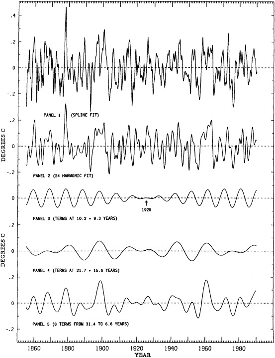
Figure 5
Global surface temperature anomaly in °C from 1855 through 1989, together with spectral oscillations derived from it determined from the maximum entropy spectrum. Panel 1: Smoothed and detrended temperature anomaly obtained by subtracting from the smooth curve of Figure 3 a spline fit to the yearly averaged anomaly data with a s of 0.106°C, as in curve 1 of Figure 4. Panel 2: Sum of 24 spectral oscillations derived from a fit to the curve in panel 1, which are consistent with the spectral peaks as listed in Table 1, column 2. Panel 3: Sum of decadal oscillations. Panel 4: Sum of bidecadal oscillations. Panel 5: Sum of eight oscillations with periods of 6.67 calendar years or greater (no exclusions). The source of the temperature data is the same as in Figure 3. The time of maximum interference of the decadal oscillations in panel 3 is indicated.
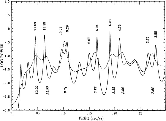
Figure 6
Two maximum-entropy spectra of the global surface temperature anomaly, expressed as power (logarithmic scale) versus frequency, in cycles per year. The temperature record used to determine the spectra was expressed as the difference between the flexible spline plotted in Figure 3 and the very stiff spline from curve "1" of Figure 4, panel 1. The solid curve indicates a spectrum with the number of poles, M, equal to 250; the dashed curve shows a spectrum with M equal to 150. The periods of the prominent peaks of the former, in years, are shown in standard characters, those of the latter by figures in italics.
Another study of nearly the same temperature record by Ghil and Vautard (1991) used a combined singular spectrum and multi-taper analysis that provides an F-test for the significance of the peaks. Their study confirms the significance, at the 97 percent confidence level, of the peaks that we found near 6, 9, 15, and 21 years, and showed evidence of several of the other peaks listed in Table 1.
Accepting the peak periods revealed by the second spectrum of Table 1 for further study, we have fit the slightly smoothed temperature record of Figure 5, panel 1, using a non-linear least-squares method (Bevington, 1969, subroutine CURFIT) to a series of sine and cosine functions having the periods indicated for peaks in the MEM spectrum, omitting only very weak peaks and any peaks with periods less than 1.7 years.
The reconstructed time series obtained by summing these 24 computed sinusoidal spectral oscillations reproduces the main peaks and troughs of the original record (Figure 5, panel 2). If individual warming and cold events are scrutinized, admittedly the fit is far from perfect. Allowing, however, that the lowest period of oscillation in the reconstruction is 1.8 years, one cannot expect a wholly consistent representation of times and amplitudes of short-term interannual fluctuations such as those related to El Niño events. As we verified by carrying out a further reconstruction using 48 harmonics that included oscillations with periods as low as 1.0 years, the correctness of the phasing and amplitudes for short-term interannual fluctuations can be improved by including higher-frequency oscillations in the fit to the temperature data. The amplitudes of the lower-frequency oscillations, which are those of importance to the present study, were only negligibly altered by the addition of higher frequencies in the fit.
The amplitudes of the sinusoidal functions are listed in Table 1. Of the 24 spectral oscillations in the reconstruction, only the two noted earlier, having periods of 9.3 and 10.2 years, occur near to the decadal time scale. Summed, these produce oscillations with an average period of 9.7 years and a maximum amplitude, peak to peak, of 0.15°C. They beat with a recurrence period of 102 years (half of the period of the long-term oscillation produced by the difference of the two shorter-period oscillations) and exhibit interference
near 1925 (Figure 5, panel 3). The pattern of interference and reinforcement is distinct because the amplitudes of the separate oscillations, as found by the least-squares fits to the sinusoidal functions, are nearly equal.
Two additional strong spectral oscillations are found in the temperature spectrum at approximately the bidecadal time scale, with periods of 15.6 and 21.7 years. Summed, they have a maximum amplitude of 0.14°C and beat with a period of 55 years (Figure 5, panel 4), which is close to half the beat period of the decadal harmonics. They also exhibit interference in the 1920s, at almost the same time as the decadal oscillations. Furthermore, their summed oscillations, with an average period of 18.1 years, essentially impose variable amplitudes on the decadal oscillations. The addition of weaker harmonics with periods of 6.7, 7.6, 12.2, and 31 years to form a broad low-pass filter of the detrended temperature record does not cancel out this beat pattern (Figure 5, panel 5). The decadal oscillations are still present, with the strongest temperature maxima where the bidecadal oscillations enhance the decadal signal. Between 1905 and 1940, however, only oscillations with periods close to 6 years appear, as was the case for the spline-fit differences of panels 2 and 4 of Figure 4.
As shown in Figure 7, the sinusoidal oscillations of Figure 5, which are derived from spectral analysis, show essentially the same patterns as those previously derived from spline fits. The decadal and bidecadal oscillations are equally prominent, whether they are obtained by spectral analysis or by the use of smoothing splines. Thus, the amplitudes and phases obtained by spectral analysis do not appear to be falsified by the restricted number of degrees of freedom of the spectral compositing.
We conclude that the decadal oscillations that have appeared in the temperature record since the late 1950s may be characteristic of the longer-term record as well. If so, the bidecadal oscillations seen in Figures 5 and 7 may also be characteristic of the longer record, especially since they appear to be an amplitude modulation of the decadal oscillations. Both pairs of oscillations are intermittent, however, being essentially absent for about 35 years near the middle of the temperature record.
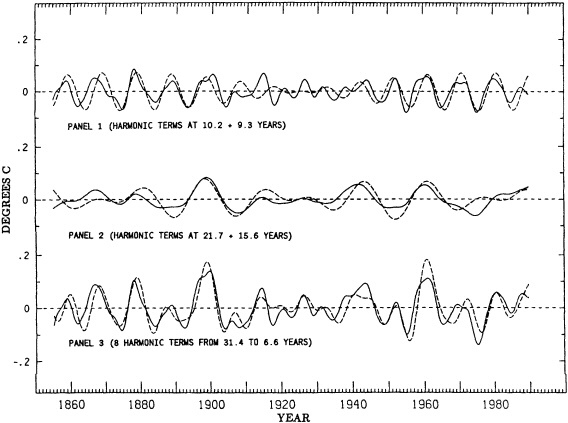
Figure 7
Spectral oscillations of the global spectrum of global surface temperature anomaly (dashed curves), compared with the same temperature record that has been band-pass filtered using spline fits (solid curves). Panel 1: Sum of decadal oscillations, as in Figure 5, panel 3, and curve "3" minus curve "2" of Figure 4. Panel 2: Sum of bidecadal oscillations, as in Figure 5, panel 4, and curve "2'' minus curve "1" of Figure 4. Panel 3: Sum of eight oscillations, as in Figure 5, panel 5, and curve "3" minus curve "1" of Figure 4.
DISCUSSION
In our quest to understand decadal oscillations that appear in the record of atmospheric carbon dioxide measurements, we have been led to investigate seemingly similar oscillations in global air temperature. Employing a much longer temperature record than that available for atmospheric CO2, we have found that decadal variations in global air temperature are characteristic of the past 135 years, except for an interval near the middle of the record. This pattern can be reproduced by assuming the existence of two oscillations with slightly different frequencies that beat on the time scale of about 100 years.
Is it possible that these decadal oscillations are caused by a cyclic process? Perceptions of cyclic behavior in the climatic record have in the past involved so many exceptions and inconsistencies that the subject does not enjoy good repute. Compelling evidence that cyclic behavior is actually caused by an identifiable forcing agent such as solar irradiance is difficult to find.
Decadal oscillations have not been emphasized in previous discussions of global temperature, but the existence of bidecadal oscillations has been alleged by Newell et al. (1989) on the basis of marine air-temperature data. An inspection of their Figure 2 indicates that the signal that they found is similar in phase and amplitude to that shown in our Figure 4, panel 4. There is no indication in their analysis of a weakened signal near 1925, however, like that found by our analysis of global air temperature. We are not aware of other finds of either decadal or bidecadal oscillations.
Of possible importance in deciding the significance of the oscillations in temperature that we report here is the indication that the decadal signal appears to be replaced by shorter oscillations, with periods of close to 6 years, from about 1905 to 1940. Although the spectral evidence for this, as shown in the low-passed record of Figure 5, panel 5, is based only on spectral peaks with periods greater than 6.5 years, the strong 6.0-year peak in the MEM spectrum produces an oscillation (not shown) with almost exactly the same phase. Thus a 6.0-year oscillation appears to be a significant contributor to the overall pattern of variability in the global temperature record, although not as prominent as the decadal signal.
The 6.0-year oscillation, and two other adjacent oscillations with periods of 4.8 and 5.2 years (see Figure 6), could well be associated with the low-frequency component of the El Niño/Southern Oscillation (ENSO) phenomenon, as pointed out by Ghil and Vautard (1991) in their spectral analysis of temperature. When these three oscillations are included in a low-frequency band-pass of temperature, warm periods in this band-passed record include most of the strong and many of the moderate El Niño events.
The 4.8- and 6.0-year oscillations, when summed, show an interference pattern with a beat period of 22.4 years. The timing of these beats shows a possible relationship to the 21.7-year spectral oscillation, inasmuch as the warm phases of this bidecadal oscillation tend to occur near the times of reinforcement of the two higher-frequency oscillations. If these higher-frequency oscillations are related to global aspects of the El Niño phenomenon, is it possible that the bidecadal oscillations that we have been discussing are also related? In the absence of a mechanism to explain any of these oscillations, and not even clear proof that they exist, it is not possible to resolve this question, but the topic appears to us to deserve further investigation.
Does the record of atmospheric CO2 provide any insight into possible causes of the interannual variations in global temperature? At first glance one would not expect so, because interannual variations in CO2 are presumably a consequence of climatic factors that do not depend on the earth's carbon cycle. Nevertheless, two aspects of the CO2 record are worth noting.
First, atmospheric CO2 anomalies show a striking relation to global temperature anomalies with respect to El Niño events (Keeling et al., 1989). Second, on all interannual time scales that can be investigated in the 32-year CO2 record up to 1990, CO2 variations tend to lag temperature variations by approximately a half-year (Kuo et al., 1990). The existence of a lag of that length on the decadal time scale is evident in the plot of Figure 1.
This lag, as shown by Keeling et al. (1989), cannot easily be explained as an oceanic phenomenon, because temperature-induced exchange of CO2 gas at the air-sea interface on a decadal time scale should result in a lag in atmospheric CO2 variation of about 1.5 years, whereas a change in upwelling of cold water should produce atmospheric CO2 variations of the opposite phase with respect to temperature, i.e., a lag of about 5 years. On the time scale of El Niño events, Keeling et al. suggest that atmospheric CO2 responds to global temperature, because vegetation on land tends to release CO2 during anomalously warm periods. With respect to this terrestrial response, a short lag in CO2 is to be expected.
Perhaps variations caused by terrestrial vegetation and driven by climatic change also produce decadal variations in CO2. Indeed, a decadal signal in CO2 might be simply a modulation in the magnitude or frequency of variations on El Niño time scales. If this should be the case, a nearly constant phase lag in CO2 with respect to temperature would be expected over a broad range of interannual frequencies, as observed.
In support of such an hypothesis are several papers' assertions of possibly non-random, long-term behavior in El Niño events. Their focus has been mainly on the decadal time scale (see, for example, Hanson et al., 1989; Michaelsen, 1989; and Enfield and Cid, 1990) but there is a hint of a decadal connection in the study of Barnett (1989),
as interpreted by Enfield and Cid. To these speculations may be added our suggestion, above, of a possible association of spectral temperature oscillations on El Niño time scales with a bidecadal oscillation.
In conclusion, we suggest that the atmospheric CO2 record may be of some use in the study of decadal variability in climate. Conclusive evidence of decadal periodicities in climatic parameters will probably be established, however, only if and when a mechanism is found that is physically reasonable and successfully predicts changes in climate.
ADDENDUM
In the oral presentation of this paper, we presented an hypothesis that forcing of ocean temperatures by oceanic tidal dissipation might explain the observed decadal oscillation in global temperature and its disappearance in the early part of this century. We were attracted to the coincidence of the times of prominent decadal temperature signal with the times when the strongest equilibrium oceanic tidal forcing was produced by the gravitational forces of the sun and moon. At these times, within 10 years of 1881 and 1974, episodes of unusually strong tidal forcing occurred at times of the strongest tides of the year, because the sun and moon tended then to be both in unusually close alignment with the Earth and at nearly closest approach. In contrast, in the 1920s, when the decadal signal was weakest, only weaker tidal forcing occurred at times of the strongest tides. Because strong tidal forcing occurs at intervals of 9 years when the alignments of the sun, moon, and earth are nearly optimal for strong tidal forcing, and otherwise at 3- and 6-year intervals, the decadal signal itself and the 6-year signal in the middle of the record period also correspond to the periodicities of tidal forcing.
It was not possible to prepare an appropriate presentation of the tidal discussion for this volume. An article describing the tidal hypothesis is in preparation.
ACKNOWLEDGMENTS
We are grateful to scientists who gave generously of their time to discuss the subjects of solar phenomena and climatic variation with us in the course of preparation of this article. We specifically thank Philip Jones and Thomas Wigley, Michael Ghil, James Hansen, Harry van Loon and Gerry Meehl, David Parker, and Henry Diaz and Thomas Karl. We are also grateful for discussions with Tim Barnett, Robert Bacastow, Daniel Cayan, and Hugh Hudson, colleagues of ours at the University of California at San Diego. We further thank Drs. Jones and Hansen for supplying us with their temperature data sets, and David Parker for supplying us with extensive global and regional sea surface temperature data in graphic form. Computer time was provided by the San Diego Supercomputer Center. Financial support came from the National Science Foundation via Grant ATM-91-21986 and from the U.S. Department of Energy via Grant FG03-90ER-60940.
APPENDIX A TABULATION OF TEMPERATURE DATA
Table A1 presents the global-average anomalies of air temperature used in our study. The anomalies are listed for each calendar month, followed in the last column by the annual average. They were obtained by averaging Northern and Southern Hemisphere anomalies. The hemispheric data for 1855 through 1989, expressed both over land and in surface seawater, were supplied to us by P.D. Jones (personal communication of April 1990). These data were supplied to us as monthly averages, whereas for 1987 through 1989 only annual averages were available with respect to temperatures in surface seawater. For these final three years of our data set we estimated global averages for each month from the monthly anomalies supplied to us for temperatures over land.
For the Northern Hemisphere we multiplied the monthly land values for each given year by the ratio of the annual global mean for that year to the mean for land. For the Southern Hemisphere we assumed that no intra-annual variations existed over the oceans, and that temperatures over land contributed 30% to the hemispheric averages. For the full data set we accepted the premise of Jones et al. (1986c) that sea surface and marine air temperatures follow each other closely on interannual time scales, so that combined land and surface sea-water-temperature data portray global-average interannual variations in surface air temperature.
Recently P.D. Jones (personal communication of April 1993) kindly supplied us with updated monthly data for all years of our study. We have repeated our calculations with these data and find only very small changes in spectral amplitudes and frequencies, and thus in the time plots shown in this article.
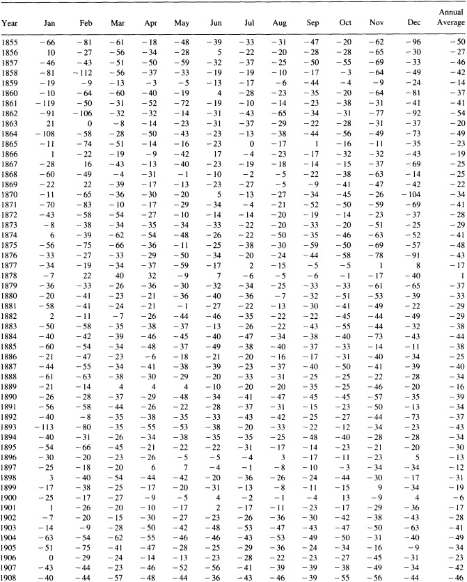
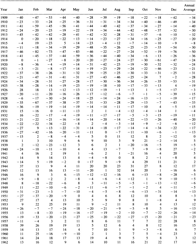
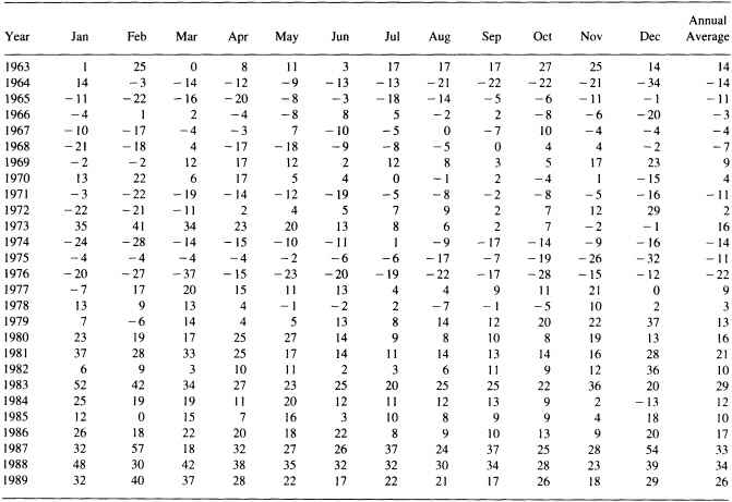
Discussion
CICERONE: I think you're touching on something very fundamental: the possibility that there may be an external source of climate variability.
TRENBERTH: It seems to me that the key question is what physical mechanism is operating here. Have you any thoughts on that, Dave?
KEELING: Well, there was a paper by John Loder and Christopher Garrett in JGR in 1978 that suggested that an 18.6-year cycle in SST can be seen on the east and west coasts of North America, of opposite phase. They found that the amount of energy involved in the tidal currents on the continental shelves might be sufficient to cause temperature changes. Peter Holloway and his colleagues have done some nice studies off the northwest coast of Australia. They find that the breaking of the internal waves eventually causes turbulence that results in so much mixing that you get an almost linear decrease in temperature from the sea surface downward. I am inclined to think that the tides are causing some sort of turbulence that affects the upper ocean.
DOUGLAS: The amplitude of the 18.6-year tide is less than a centimeter. It's very difficult to detect in the tide-gauge records. Where does all the energy go?
KEELING: I think the semi-diurnal and diurnal tides would have to carry most of the energy dissipation. What strikes me is that if you look at the correlation of cooling with the tides themselves, you see that the greatest amount of cooling tends to occur in conjunction with a strong tide.
GHIL: I find it interesting that, using an entirely independent technique, Dave is getting results that are nearly identical to those that I and Robert Vautard published in Nature in March 1991. We had peaks at similar locations, including a 15-to-16-year one.
KEELING: The 15-year one seems to me to be the best candidate for some sort of tidal connection because it is not explained by any kind of solar activity.
Observed Variability of the Southern Hemisphere Atmospheric Circulation
DAVID J. KAROLY1
ABSTRACT
The dominant modes of interannual variation of the Southern Hemisphere (SH) circulation are described, using results from several studies of grid-point analyses of the SH troposphere. The two leading modes are primarily zonally symmetric, representing out-of-phase variations of height between middle and high latitudes in one case (called the high-latitude mode) and between the tropics and middle latitudes in the other (called the low-latitude mode). Wave-train patterns of anomalies are described also. These include a wave-number-three mode in winter with large amplitude at high latitudes, a wave-number-four mode in middle latitudes in summer, a meridional wave-train structure originating over Australia, and a monopole or a meridional wave train over the Pacific Ocean in winter. The two most important processes leading to interannual variations of the SH circulation appear to be the Southern Oscillation and the interaction between waves and mean flow in the SH storm track, which leads to the High Latitude mode.
Since upper-air data and grid-point analyses are available for only a short period, surface data must be used to describe decadal variability of the SH circulation. The barotropic vertical structure of low-frequency variations in the SH means that surface pressure variations are representative of variations throughout the troposphere. Relatively little attention has been paid to decadal variability in the SH. It appears from indices of the two dominant modes of interannual variations, determined using the surface data, that the modes show substantial decadal variability over the last 90 years. Few observational data exist that can be used to directly indicate climate variability on century time scales in the SH. The only possible observational evidence for this comes from proxy data, such as tree rings.
INTRODUCTION
There has been relatively less study of the variability of the Southern Hemisphere (SH) atmospheric circulation than of that of the Northern Hemisphere (NH). There are a number of reasons for this; the lower population and greater ocean areas in the SH mean that observational records are sparser and there have been fewer people to analyze them. In this brief and incomplete review, I will concentrate on studies of the variability of the SH tropospheric circulation, starting at interannual time scales and moving onto longer time scales. This progression is justified by the available observational data and the number of relevant studies, as outlined below.
Detailed and regular observations of the troposphere over much of the SH did not start until the International Geophysical Year in 1957-1958, when the number of SH upper-air sounding stations increased markedly. Operational subjective analyses of the SH circulation have been prepared since that time by the Australian and South African weather services. The introduction of meteorological satellites in the late 1960s led to the development of the first operational objective numerical-analysis scheme for the SH at the Australian Bureau of Meteorology in 1972. Hence, objective numerical analyses for the SH are available for only the last 20 years, and upper-air sounding data are available for only about 30 years.
Hemispheric numerical analyses have been used to investigate the interannual variability of the SH circulation, particularly over the last decade (Trenberth, 1979; Rogers and van Loon, 1982; Mo and van Loon, 1984; Mo and White, 1985; Kidson, 1988a,b; Karoly, 1989a; and others). In addition, radiosonde station data have also been used for similar investigations by Szeredi and Karoly (1987a,b). The results of these studies of the dominant modes of variability of the SH circulation on interannual time scales are summarized in the next section.
Since these upper-air data are available for a short period only, it is not possible to use them to describe variations on decadal time scales or longer. There are longer records of surface meteorological observations for SH stations, some extending back to before the turn of the century. The equivalent-barotropic vertical structure for the low-frequency tropospheric variations (Szeredi and Karoly, 1987a) permits these surface records to be used to provide some information on decadal variability in the SH. However, there have been no comprehensive studies of decadal time-scale variability for the SH. More recently, Jones (1991, hereafter referred to as J91) has reconstructed from station data a gridded mean sea-level pressure data set for the SH that extends back to 1911. J91 and Allan and Haylock (1993) have used this data set to consider decadal variations of the SH circulation. These and a few other studies of long surface records are described briefly below, although the others have generally concentrated on variations of El Niño and the Southern Oscillation.
In an attempt to provide some evidence of the range of SH variability on century time scales, some climate reconstructions based on proxy data are discussed below. Although these proxy data are available for very few sites in the SH, they constitute the only source of data on natural climate variability on century time scales for the SH. More extensive descriptions of proxy data for the SH are provided in Chapter 5 of this volume.
INTERANNUAL VARIATIONS FROM UPPER-AIR DATA
Relatively less attention has been paid to low-frequency variations of the SH circulation than to those of the NH, probably because of the shorter time period for which analysis data sets are available. Trenberth (1979), Kidson (1988a), and Shiotani (1990) have used zonal-mean data to show that there are large low-frequency variations of the zonal-mean circulation in the SH involving variations of the zonal wind and associated dipole variations of geopotential height. Mo and White (1985, hereafter referred to as MW) carried out a teleconnection analysis for the SH (similar to that of Wallace and Gutzler (1981) for the NH) using 8 years of monthly mean SH analyses. From their grid-point correlation maps, they identified three modes of variation: a zonally symmetric dipole mode at middle to high latitudes, a zonal wave-number-three mode in winter, and a continent-ocean contrast in summer. Szeredi and Karoly (1987b, hereafter referred to as SK) used the longer period of upper-air station data available for the SH (up to 30 years) to investigate low-frequency variations. They found two dominant modes of monthly variation in the station data that were primarily zonally symmetric, involving opposing departures of height between middle and high latitudes in one case and between the tropics and middle latitudes in the other. The sparse and irregular station network in the SH meant that only the largest-scale modes could be identified.
More recently, the technique of unrotated and rotated principal-component analysis (PCA) has been applied to grid-point analyses of the SH to clarify the typical modes of low-frequency variations of the SH circulation in a number of different studies. These may be separated into two groups according to the time scale of interest: Periods longer than about 50 days, including interannual variations, have been considered by Rogers and van Loon (1982), Kidson (1988b, hereafter referred to as K88), and Karoly (1989b), while another group concentrated on intraseasonal variability. The results are similar for different studies of the same time-scale fluctuations, and differences can usually be explained in terms of differences in analysis method, such as PCA of the correlation (Karoly, 1989b) or covariance matrix (K88), use of different variables (300 hPa height by
Karoly (1989b), 500 hPa height in most other studies), differences in time filters used, or seasonal stratification. The main data sets used have been the Australian SH analyses, available since 1972 (Karoly, 1989b; Rogers and van Loon, 1982; MW) and the European Centre for Medium-range Weather Forecasts (ECMWF) analyses (K88 and many intraseasonal studies), which are available only for 1979 and later but are likely to be of higher quality than the Australian analyses.
In the following discussions, the typical modes of interannual variations are described first, using results from Karoly (1989b). A rotated PCA has been carried out on monthly anomalies of 300 hPa height using 15 years of Australian analyses (1973-1987). Three different types of horizontal structure have been identified for the low-frequency variations in the SH. The leading modes are approximately zonally symmetric, occur in both summer and winter, and explain about a quarter of the variance. They are associated with opposite departures of height for middle compared with high latitudes and for the tropics compared with middle latitudes. The other stable modes are hemispheric-scale wave-like variations, either zonal wave trains around the hemisphere or regional meridional wave trains, both of which seem to be less important than the symmetric modes. All the modes have an equivalent-barotropic vertical structure in the extratropics, and generally are more horizontally extensive than the typical modes of low-frequency variation in the Northern Hemisphere. The equivalent-barotropic vertical structure of low-frequency variations in the SH was identified using radiosonde data by Szeredi and Karoly (1987a).
Zonally Symmetric Modes
The two leading modes from the rotated PCA of monthly anomalies of 300 hPa height are mainly zonally symmetric, representing opposite height variations over different latitude bands. These modes are found in both summer and winter. One mode represents a north-south out-of-phase variation of height between Antarctica and middle latitudes; it will be referred to hereafter as the high-latitude mode. The horizontal structure of this mode is shown in Figure 1a for winter, using correlations of the time series of PC scores for this mode with monthly SH height anomalies. The proportion of the total monthly variance explained by this mode is about 12 percent. Although it is primarily zonally symmetric, there are substantial asymmetries, with larger correlations and gradients over the Indian Ocean and south of Australia. The middle latitudes show evidence of zonal asymmetry resembling a wave-number-three pattern. This high-latitude mode has an equivalent-barotropic vertical structure with very similar variations in both 500 hPa height and MSLP.
This mode of low-frequency variation in the SH has
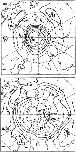
FIGURE 1
Rotated principal-component patterns for monthly 300 hPa height anomalies in winter representing the two leading modes, (a) high-latitude mode and (b) low-latitude mode. Correlations of the time series of the PC scores with monthly anomalies are shown.
been identified by SK using station data; by Rogers and van Loon (1982), MW, and K88 using shorter time periods of analyses; by Shiotani (1990), Kidson (1988a), and Trenberth (1979) using zonal-mean fields; and by Trenberth and Christy (1985) using zonal-mean surface pressure. SK found that it was the second mode of monthly variations of the station data, explaining a smaller fraction of variance than
here, whereas K88 found that it was the leading mode of interannual variations of 500 hPa height in the ECMWF analyses. Kidson (1988a) has shown that this mode occurs on all time scales from intraseasonal to interannual.
The other mode found in both seasons represents an out-of-phase north-south variation of height between low and middle latitudes; it is shown in Figure 1b for winter. This mode, hereafter referred to as the low-latitude mode, explains about 13 percent of the variance in winter. Strong departures from zonal symmetry occur in the South American region, with the nodal line running almost parallel to the coast. More intraseasonal variation than interannual variation is found for this mode in winter, but in summer it is mainly associated with interannual variations.
Structures similar to this low-latitude mode have been identified by SK using station data and by Kidson (1988a) using zonal mean wind fields. This mode in the station data explains a larger fraction of variance than here, probably because of the more northerly extent of the analysis region in SK. K88 did not identify this mode, probably because his analysis using the covariance matrix of 500 hPa height variations is restricted to patterns that have large-amplitude anomalies at that height, whereas they are generally small in low latitudes.
MW presented a correlation analysis of the monthly zonal mean height and MSLP fields from their data set (refer to their Figures 1 and 2). They found structures in the zonal-mean fields that are similar to the zonally symmetric modes described here. The two leading modes for the zonal-mean fields, which explain about 70 percent of the variance, have see-saw structures over latitude bands similar to the high-latitude and low-latitude modes shown in Figure 1.
Wave Trains
In addition to the zonally symmetric structures, wavelike patterns were also found in the PCA. They explain less variance and are less stable than the zonally symmetric modes, but are found in one-point correlation maps and composite analyses. In contrast to the NH wavelike modes, the modes found in the SH exert influence over hemispheric scales. They include zonal wave-number-three patterns and meridional wave trains in winter, and wave-number-four patterns or continent/ocean contrasts in summer.
Two stable zonal wave-number-three patterns were found for winter 300 hPa height; they are shown in Figure 2. The centers of action are located at around 60°S for the first version and about 50°S for the second version. The main difference between the two patterns is that one is shifted by about one quarter wavelength relative to the other, so that the extrema of one occur along the nodal lines of the other. The second version shows a stronger relationship (out-of-phase relative to the main centers) with lower latitudes, while the first version shows evidence of a weak
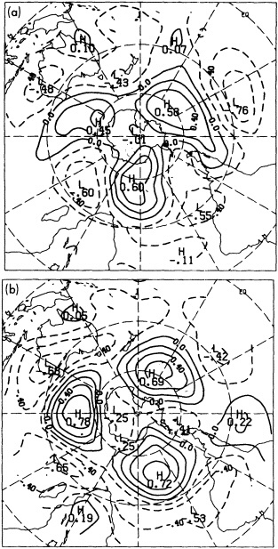
FIGURE 2
Rotated PC patterns of winter 300 hPa height in winter describing the two versions of the wave-number-three mode, as in Figure 1.
wavenumber-four structure at around 30°S. About 7 percent of the variance is explained by the first version, while the second explains about 5 percent of the variance. Together, wave-number-three patterns represent about 12 percent of the variance, a total similar to that of each of the zonally symmetric modes.
Using one-point correlation maps, MW identified a zonal wave-number-three pattern in the SH winter. The two orthogonal versions of the mode found here, with large amplitude at high latitudes, indicate that zonal wave-number-three
anomalies are a common low-frequency pattern in the SH, but that they do not have a strongly preferred phase. Mo and van Loon (1984) describe a change in the amplitude of wave-number-three on long time scales.
As well as the zonal wave-number-three pattern in winter, two versions of a zonal wave-number-four pattern were found in summer that are phase-shifted with respect to each other. Together these modes explain about 13 percent of the summer height variance. They both have centers of action around 45°S and show a continent-ocean contrast. MW identified a teleconnection pattern in the SH summer associated with the continent-ocean thermal contrast; this pattern appears to be related to this zonal wave-number-four pattern found in the upper troposphere.
A meridionally oriented standing-wave pattern resembling a wave train has been found in winter. The pattern for this winter wave train is shown in Figure 3a. Five centers of action can be seen extending from eastern Australia southeastward to high latitudes and equatorward into the southern Atlantic. This mode, which explains about 6 percent of the variance, is not clearly evident in the lower-level variables, where only parts of the wave-train structure are reproduced. Using low-pass filtered ECMWF analyses, however, K88 has identified a similar wave-train pattern of height variations.
The third principal component of 300 hPa height in winter explained a relatively large fraction of the variance, but was not stable; it displayed different structures when different analysis methods were used. The pattern for this mode, shown in Figure 3b, essentially represents monopole height variations over the Pacific Ocean, although there is some indication of opposite variations further equatorward and poleward, suggesting a meridional wave train. Although the feature over the central Pacific was relatively stable, the weaker features in this pattern were quite variable.
Mechanisms
Although the above studies have described low-frequency variations in the SH, much less attention has been paid to the mechanisms associated with these observed variations. Karoly (1989a,b) and SK have shown that the interannual variations of the low-latitude mode in summer are are related to the Southern Oscillation and the associated variations of the temperature of the tropical troposphere. In winter, the Southern Oscillation is associated with a pattern of large-amplitude anomalies over the Pacific Ocean, as shown in Figure 3b. Hence the Southern Oscillation is associated with two of the dominant modes of interannual variability in the SH.
The other common interannual variations in the SH are linked to the high-latitude mode. K88, Karoly (1990), and Shiotani (1990) have shown that the zonally symmetric variations of the high-latitude mode are associated with
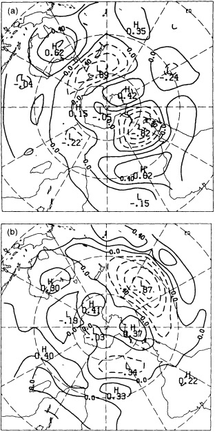
FIGURE 3
Rotated PC patterns for 300 hPa height in winter for the two meridional wave-train modes.
changes in the observed transient-eddy activity and momentum flux in the SH storm track. Trenberth (1984) showed that the large circulation anomalies during the SH winter of 1979, during the Global Weather Experiment, were related to mean flow and eddy variations associated with this high-latitude mode. A general-circulation modeling study of Zwiers (1987) found that the largest interannual variations of the model SH circulation were zonally symmetric opposite variations between high and middle latitudes, very similar to those of the observed high-latitude mode. Simplified
atmospheric-modeling studies by James and James (1989) and Robinson (1992) have shown that it is also the dominant mode of low-frequency variations in extended simulations with simplified general-circulation models with zonally uniform boundary conditions. Hence, this zonally symmetric high-latitude mode appears to be a ubiquitous mode of low-frequency variation of the SH, associated with interaction between the mean flow and the transient eddies in the SH storm track.
Little study has been made of the zonal wave-train modes, but it is likely that the quasi-stationary interannual wave-number-three modes are associated with the three SH land masses and continent-ocean thermal contrasts. In addition, the zonal wave-number-three Rossby wave is almost stationary in the mean SH zonal wind in mid-latitudes.
INTERDECADAL VARIATIONS ASCERTAINED FROM SURFACE DATA
Since upper-air observations are available for the SH for about three decades only, it is not possible to use such data to describe the interdecadal variations of the SH circulation. The only analyses of longer-term variations of the SH troposphere using upper-air station data have concentrated on temperature trends (Angell, 1986; Karoly, 1987). These have shown a small warming trend in the SH lower troposphere over the last three decades.
Some evidence of longer-term changes in the SH circulation is found when the mean sea-level pressure analyses prepared by the South African Weather Bureau for 19511958 (Taljaard et al., 1961) are compared with analyses from the Australian Bureau of Meteorology from 1972. Although some differences are due to different analysis methods, some pressure changes appear to be real (Mo and van Loon, 1984; J91).
The equivalent-barotropic vertical structure of low-frequency variations in the SH (Szeredi and Karoly, 1987a) means that longer records of surface observations may be used to describe interdecadal variations. Surface-pressure observations are available for some SH stations for periods extending back to the last century, and sea surface pressure observations over limited SH ship tracks are available for a similar period. It should be noted that these records are often incomplete and are representative of only limited SH regions.
J91 has used station data to reconstruct gridded SH mean sea level pressure (MSLP) fields for most of this century. The quality of this MSLP data set has been assessed by J91 and Barnett and Jones (1992). It is considered to be of reasonable quality over the region 15°S to 60°S from 1951 on, but the reconstructions back to 1911 are useful only near the continents and over the southwestern Pacific Ocean. Jones has used these data to assess changes since 1951 in the strength of the three subtropical anticyclones and the southern high-latitude westerlies; time series of indices of the strength of the South Pacific anticyclone and the high-latitude westerlies from J91 are shown in Figure 4. They
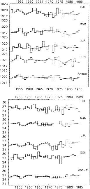
FIGURE 4
Seasonal and annual time series of two indices of the SH circulation: upper panel, South Pacific anticyclone high (average pressure in the region 25°S to 35°S, 80°W to 110°W); lower panel, strength of the high-latitude westerlies (zonal-mean pressure difference 40°S to 60°S). The filtered curve is from a 13-term Gaussian filter designed to suppress variations on time scales less than 10 years. (From Jones, 1991; reprinted with permission of the Royal Meteorological Society.)
show large interannual variations, as well as some fluctuations on decadal time scales. The interannual variations of the South Pacific anticyclone are associated with the Southern Oscillation, and they are larger than those of the anticyclones over the other two SH ocean basins. The index used for the strength of the southern westerlies is also a measure of the high-latitude mode described earlier. It shows pronounced interannual and longer-term variations.
Allan and Haylock (1993) have used the J91 MSLP data set to identify the SH circulation variations associated with the long-term winter rainfall decrease over southwestern Australia. In the Australasian region, they describe variations of MSLP on decadal time scales as well as a longer-time-scale trend, both of which are associated with the regional rainfall variations.
Several indices of the large-scale surface-pressure field in the SH have been used to investigate variations of the SH circulation (Troup, 1965; Trenberth, 1976; Pittock, 1984). The index most frequently used is the Southern Oscillation Index (SOI), the difference between normalized mean sea-level pressure anomalies for Tahiti and those for Darwin. This index represents the magnitude of the pressure oscillation between the eastern Pacific Ocean and Indian Ocean regions associated with the Southern Oscillation. Pittock (1984) defined the Trans-Polar Index (TPI) as the pressure anomaly at Hobart (43°S, 147°E) minus that at Stanley (52°S, 58°W), on the opposite side of the hemisphere. The TPI represents variations of the amplitude of zonal wave-number-one asymmetries in the pressure field. It probably captures variations in the high-latitude mode to some extent, because of the difference between the latitudes of the two stations. Pittock (1984) has shown that the two dominant modes of common interannual variations of rainfall in Australia, New Zealand, South Africa, and South America are associated with variations of the SOI and the TPI, and that there is little relationship between these two indices. Pittock considered only 30 years of data, 1931 to 1960, and did not directly examine interdecadal variations of these indices and hence of the SH circulation. However, in commenting on several other studies that have considered relatively long time series of the SOI, he noted that there were significant differences in the relationship between the SOI and Australian rainfall between the periods 1930 to 1950 and 1950 to 1980, with a much weaker relationship in the 1930-to-1950 period.
Several recent studies (Hamilton and Garcia, 1986; Elliott and Angell, 1988; Allan et al., 1991; Quinn and Neal, 1992) have examined decadal variability of the Southern Oscillation; it is covered in some detail in Cane et al. (1995), Keeling and Whorf (1995), Rasmusson et al. (1995), and Trenberth and Hurrell (1995), all in this volume. It is sufficient to say here that decadal variations in the Southern Oscillation must be associated with significant decadal variations in the SH circulation.
Time series of the SOI and the TPI since 1896 are shown in Figure 5. There is negligible correlation of the interannual variations between these two time series over the past century, confirming the conclusion of Pittock (1984) that they represent independent modes of variation of the SH circulation. The SOI and TPI show large interannual fluctuations as well as variations on longer time scales. The TPI exhibits decadal variations that are a larger fraction of its interannual variability than does the SOI. The decadal time-scale variations of these two indices must be associated with variations of the SH circulation on these time scales and, almost certainly, with regional climate fluctuations as well.
LONGER-TIME-SCALE VARIATIONS FROM PROXY DATA
It is not possible to use the available surface meteorological observations for the SH to describe variations at century or longer time scales in the SH. The only source of data at these longer time scales is proxy data from tree rings or other sources from a very few sites in the SH. Cook et al. (1991) and Villalba et al. (1989) have used tree rings to reconstruct temperature variations at some SH sites, while Lough and Fritts (1990) have used tree rings to identify
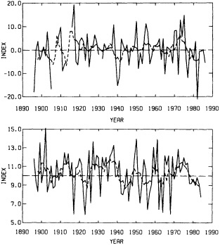
FIGURE 5
Variations of two surface-pressure indices of the SH circulation, with the solid line joining annual values and the dashed line 5-year running averages. Upper panel, Southern Oscillation Index (SOI), normalized Tahiti—Darwin pressure anomalies. Lower panel, Trans-Polar Index (TPI), Hobart-Stanley pressure differences.
SOI fluctuations over several centuries. The temperature reconstructions show marked variability on decadal time scales. The tree-ring temperature reconstruction for Tasmania by Cook et al. (1991) shows a pronounced warming trend over the last few decades, which is consistent with sea surface temperature variations in the SH and in this region over the same period (Folland et al., 1990). The tree-ring series from Tasmania is discussed further in this volume by Cook et al. (1995).
Other proxy evidence of climate variability in the SH has been obtained from coral growth rings (Isdale, 1984), geological lake-level records (Kotwicki and Isdale, 1991), ice cores (Thompson et al., 1984), river-flow records (Wells, 1987; Whetton et al., 1990) and from a variety of sources (Markgraf et al., 1992). In general, however, it is difficult to directly relate these regional proxy data directly to large-scale climate variability in the SH. They provide an indication of the range of climate variability in the source regions for the data. Further work is required to determine the representativeness of some of these regions for the climate of the whole SH.
SUMMARY
The dominant modes of intermonthly and interannual variation of the SH circulation have been described using results from several studies of grid-point analyses of the SH tropospheric circulation. The two leading modes are primarily zonally symmetric, representing out-of-phase variations of height between middle and high latitudes in one case (called the high-latitude mode) and between the tropics and middle latitudes in the other (called the low-latitude mode). These two modes, which explain almost a quarter of the variance of monthly mean 300 hPa height in the SH in both summer and winter, have large interannual variations. The dominance of these zonally symmetric modes by comparison with wavelike or regional patterns in the SH is in contrast to what is typical in the NH. Wave-train patterns of anomalies are also found in the SH circulation. These include a wave-number-three mode in winter with large amplitude at high latitudes, a wave-number-four mode in middle latitudes in summer, a meridional wave-train structure originating over Australia, and a monopole or meridional wave train over the Pacific Ocean in winter. The two most important processes leading to interannual variations of the SH circulation appear to be the Southern Oscillation and the wave, mean-flow interaction in the SH storm track, which leads to the high-latitude mode.
Since upper-air data and grid-point analyses are available for only a very short period in the SH, surface data must be used to describe decadal variability of the SH circulation. Because of the barotropic vertical structure of low-frequency variations in the SH, the surface-pressure variations are representative of variations throughout the troposphere. Relatively little attention has been paid to decadal variability in the SH. It appears from indices of the two dominant modes of interannual variations, determined using surface data, that the modes show substantial decadal variability over the last 90 years.
There are few observational data that can be used directly to indicate climate variability on century time scales in the SH. The only possible observational evidence for this is proxy data, such as tree rings.
ACKNOWLEDGMENTS
This brief review represents my own perspective on studies of observed variability of the SH circulation. It is incomplete, and I apologize for any omissions. I wish to thank Phil Jones for providing Figure 4 and the station data for generating the time series of the TPI in Figure 5, Rob Allan for allowing access to his detailed bibliography on ENSO, and my many colleagues around the world who have provided stimulating discussions on the SH circulation over a number of years. This review was supported in part by a Dedicated Greenhouse Research Grant from the Australian National Greenhouse Advisory Committee. I am grateful to the U.S. National Research Council for the invitation to prepare this brief review.
Commentary on the Paper of Karoly
David E. Parker
U.K. Meteorological Office
I was particularly interested in Dr. Karoly's video, which raises several questions. I think it would be possible to verify and improve his land-based analyses, because we have large numbers of marine data that we at the Met Office, and Henry Diaz and others at NCAR, are hoping to put together in a blend of our marine data bank and the COADS data base. The COADS data and ours include pressures and winds, so that they can be checked against one another. They should be a good method of filling in this area of the world, which is not very well covered with observations.
Some of you may also have read Neil Ward's work (J. Climate, 1992) in which he corrects marine winds. The measured winds appear to have become stronger relative to the geostrophic winds calculated from the pressures. So far, this work has gone back only to 1949, although similar work could be carried out for earlier years. It is very labor-intensive, but one of my recommendations is that the Southern Hemisphere surface data base be improved. An improved surface data base, especially in the Southern Hemisphere, might help us better understand the mechanisms of climate. For example, Section C of the 1992 IPCC Science Supplement shows what happens to estimates of trends in oceanic latent heat fluxes if we apply appropriate corrections to the winds.
Unfortunately, many of the upper-air data from Southern Hemisphere rawinsonde stations are missing, e.g., in Brazil, Antarctica, and southern tropical Africa. I would therefore recommend that everything be done to maintain the network, especially in developing countries and on remote islands. The other problem with the upper-air data is that changes of instrument type and changes of operating practice must be compensated for. To do this, we need adequate station histories. These, as well as the data, are being collated in the Comprehensive Aerological Reference Data Set (CARDS) project under Tom Karl and others at Asheville.
Ultimately, of course, the adjusted data should be put together in a fixed-model-based reanalysis, to yield self-consistent analyses. This is being done by the European Centre for Medium-range Weather Forecasting, and data back to 1958 are being analyzed at NOAA/NMC.
And last, the South Pacific Convergence Zone is an intriguing phenomenon, and vital to our understanding of the Southern Hemisphere climate. So, extra effort should be made to measure and understand it.
Discussion
GHIL: You called your first two EOFs high latitude and low latitude, but what matters is where the nodal line is. Perhaps you have pools of air trapped behind the high-latitude and subtropical jets that happen to have different temperature anomalies.
KAROLY: The interaction between the storm tracks and the main jets is a complicated process that can lead to long-lived low-frequency anomalies. The general symmetry of the anomalies is perhaps more characteristic of the Southern Hemisphere because of the topography. But I agree that it could be described in terms of symmetric air-mass contrast between warmer and colder regions.
GROOTES: Ice-core records for different parts of Antarctica might be able to give you an idea of whether this kind of circulation persisted.
SHUKLA: In the video you showed, almost all the major fluctuations around Australia were coming from the south. Was that a data problem?
KAROLY: It looks that way until the 1950s, but then till the 1970s or 1980s they seem to come more from the north and after that there is no obvious signal. I imagine it's a data problem, but the only way to know is to look at the individual station data. I'm hoping to persuade Phil Jones to do some analysis of this.
TRENBERTH: The dominant mode in the Southern Hemisphere is a double jet structure, with the jets alternating in strength. This mode has been simulated by the Canadian Climate Center and by the Japanese, and in fact turns out to be the dominant global mode. It is entirely derived from natural variability, and seems to have no connection to any external forcing.
KAROLY: It's not clear that internal fluctuations in the atmosphere alone can provide enough longevity to extend it into the decadal range. There might be a link with the Antarctic circumpolar current or the distribution of ocean temperature in the Southern Hemisphere that could provide a longer duration. The Max Planck Hamburg model produces a 50-year episode of this mode, as I remember. It is internal to these sorts of models.
Surface Climate Variations over the North Atlantic Ocean During Winter, 1900-1989
CLARA DESER1 AND MAURICE L. BLACKMON2
ABSTRACT
The low-frequency variability of the surface climate over the North Atlantic during winter is described, using 90 years of weather observations from the Comprehensive Ocean-Atmosphere Data Set. Results are based on empirical orthogonal function analysis of four components of the climate system: sea surface temperature (SST), air temperature, wind, and sea level pressure. An important mode of variability of the wintertime surface climate over the North Atlantic during this century is characterized by a dipole pattern in SSTs and surface air temperatures, with anomalies of one sign east of Newfoundland, and anomalies of the opposite polarity off the southeast coast of the United States. Wind fluctuations occur locally over the regions of large surface-temperature anomalies, with stronger-than-normal winds overlying cooler-than-normal SSTs. This mode exhibits variability on quasi-decadal and biennial time scales. The decadal fluctuations are irregular in length, averaging about 9 years before 1945 and about 12 years afterward. There does not appear to be any difference between the wind-SST relationships on the different time scales.
Another dominant mode of variability is associated with the global surface warming trend during the 1920s and 1930s. The patterns of SST and air temperature change between the periods 1900-1929 and 1939-1968 indicate that the warming was concentrated along the Gulf Stream east of Cape Hatteras. Warming also occurred over the Greenland Sea and the eastern subtropical Atlantic. The warming trend was accompanied by a decrease in the strength of the basin-scale atmospheric circulation (negative phase of the North Atlantic Oscillation). In marked contrast to the dipole pattern, the wind changes occurred downstream of the largest SST anomalies. Hence the gradual surface warming along the Gulf Stream may have been a result of altered ocean currents rather than of local wind forcing.
INTRODUCTION
Climate variability on decadal and longer time scales is a subject of increasing interest and relevance. Concern over anthropogenic effects on global climate provides a strong impetus to describe and understand the natural modes of variability of the climate system. In this study, we focus on the low-frequency climate fluctuations over the North Atlantic Ocean since the turn of the century.
The North Atlantic is a region of particular importance to the global climate system. The formation of bottom water at high latitudes of the North Atlantic drives a trans-equatorial thermohaline circulation. Changes in the rate of deep-water production south of Iceland (and hence in the strength of the thermohaline circulation) can have a profound effect on global climate, as can be inferred from paleoclimate data (Broecker et al., 1986; Lehman and Keigwin, 1992) and as is shown by the modeling studies of Rind et al. (1986) and Manabe and Stouffer (1988). Recent ocean modeling experiments indicate that self-sustained oscillations of the thermohaline circulation can occur on decadal and longer time scales (Weaver and Sarachik, 1991).
Low-frequency climate fluctuations in the North Atlantic since World War II have been investigated in several studies. Levitus (1989) used subsurface measurements of temperature and salinity to document a major shift in the ocean circulation in the North Atlantic between the late 1950s and the early 1970s. Knox et al. (1988) showed that the Northern Hemisphere atmospheric circulation experienced an abrupt transition during the early 1960s (see also Flohn, 1986; Shabbar et al., 1988). One of the best-documented examples of low-frequency variability at high latitudes of the North Atlantic is the Great Salinity Anomaly, a freshwater mass that was observed to travel around the subpolar gyre from 1968 to 1982 (Dickson et al., 1988). The freshening of the surface waters was sufficient to halt temporarily deep-water formation in the Labrador Sea (Lazier, 1980). Mysak et al. (1990) discuss the relationship between the Great Salinity Anomaly and interdecadal oscillations in the Arctic climate system.
Studies dealing with the longer (100-year) marine records have tended to emphasize globally averaged surface-temperature variations (cf. Paltridge and Woodruff, 1981; Jones and Kelly, 1983; Barnett, 1984; Folland et al., 1984; Jones et al., 1986c). These studies find that the dominant signal in worldwide temperatures is a warming trend from about 1920 to 1940, with the largest amplitudes at high latitudes.
Bjerknes (1959, 1961, 1962, 1964) investigated air-sea interaction in the North Atlantic on time scales ranging from interannual to interdecadal. Using data from 1890 to 1940, Bjerknes provided compelling evidence that interannual fluctuations in SST are largely governed by wind-induced changes in latent and sensible heat fluxes at the sea surface. However, the long warming trend during the first quarter of this century appears to be linked to a change in the ocean circulation rather than to air-sea energy fluxes (Bjerknes, 1959). Similar conclusions regarding interannual and interdecadal SST variations are reached by Kushnir (1994).
The purpose of this study is to describe the variability of the winter climate over the North Atlantic Ocean, using 90 years of surface marine data. The North Atlantic is the only ocean basin with data coverage that is sufficiently dense for a regional study of climate change since 1900. We focus on the winter season because (1) the atmosphere-ocean coupling is most vigorous and (2) the SST variations reflect significant heat-content anomalies in the upper ocean. We are particularly interested in whether the climate system exhibits preferred time scales of variability, and whether the atmosphere-ocean relationships change with spectral frequency. Our results are based on an objective (empirical orthogonal function) analysis of four components of the climate system: SST, air temperature, wind, and sea level pressure. We will show that the surface climate over the North Atlantic exhibits coherent decadal fluctuations that resemble the variations on interannual time scales. The decadal fluctuations appear to be closely related to sea-ice extent in the Labrador Sea. We will also show that the Gulf Stream was apparently involved in the long-term warming trend during the 1920s to 1930s.
The data and methods are described; the two leading modes of surface-temperature variability during the period 1900 to 1989 and their relation to the atmospheric circulation are documented; and the results are discussed.
DATA AND METHODS
Data
The surface wind, sea level pressure, SST, and surface air temperature data used in this study are from the Comprehensive Ocean-Atmosphere Data Set (COADS), an extensive compilation of weather observations from merchant ships (Woodruff et al., 1987). We have used data gridded by 4° latitude/longitude squares for the period 1900 to 1989. The COADS data are uncorrected for changes in instrumentation, observing practice, ship type, etc. Spurious trends resulting from these changes have been reported in surface wind speed and SST over the tropical oceans (Ramage, 1987; Wright, 1988; Cardone et al., 1990). Our approach to the issue of whether the routine ship-based measurements are sufficiently accurate and homogeneous to allow the detection of real climate signals is to demonstrate physical consistency among independent variables: wind patterns are compared to pressure distributions, and SST fields to surface air temperatures.
Methods
The monthly mean data were converted to anomalies by subtracting long-term monthly mean values for the period 1900 to 1989. These monthly anomalies were then averaged
into seasonal anomalies (November to March) to form winter-mean departures from normal. The winter-mean value was considered missing if two or more months in a winter were missing. Missing data have not been replaced.
Empirical orthogonal function (EOF) analysis was used to identify objectively the dominant modes of variability in the North Atlantic climate system during the period 1900 to 1989. EOF analysis was performed separately on the SST, air temperature, sea level pressure, and zonal wind fields. EOFs were calculated using only those grid squares with at least 60 years of winter-averaged data. A minimum of 50 grid squares containing data in each winter was required for reconstructing the principal components (time series of the EOFs).
RESULTS
EOF Modes of Surface Temperature Variability
Figure 1 shows the first two EOFs of SST over the North Atlantic, superimposed on the long-term mean SST distribution. The EOFs are based on un-normalized winter-mean (November to March) anomalies during the period 1900 to 1989. The first EOF (Figure 1a; hereafter referred to as E1 SST), which accounts for 45 percent of the variance, has uniform polarity over the entire basin. The largest loadings occur along the Gulf Stream (as indicated by the tightly packed isotherms in the climatology). The time series of E1 SST (Figure 1b) exhibits a sudden transition from below-normal values to above-normal values around World War II. It is well known that the technique for measuring SSTs aboard ships changed during the early 1940s, and that the bucket temperatures used before World War II were about 0.3° lower than the engine intake samples used later (cf. Wright, 1986; Folland et al., 1984). Over the Gulf Stream this difference can reach approximately 0.8°, due to the rapid evaporative cooling from the bucket samples (Bottomley et al., 1990). Thus, one may be tempted to disregard El SST; however, air temperatures exhibit a similar EOF pattern with a more realistic time series (see below).
The second EOF (Figure 1c; hereafter E2 SST), which
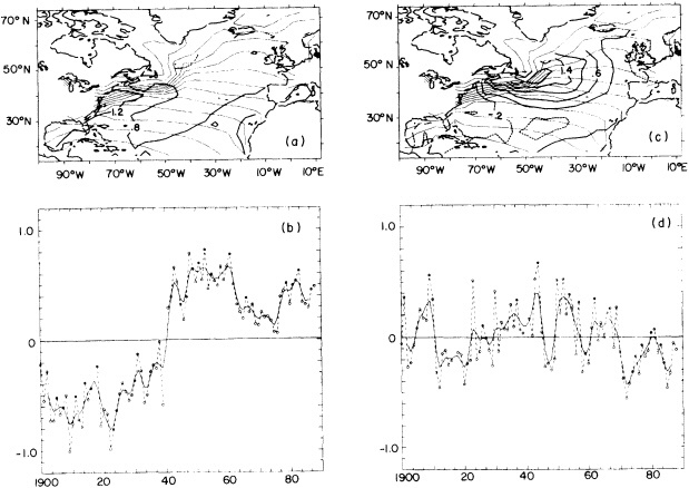
FIGURE 1
(a) EOF 1 of North Atlantic SST anomalies based on un-normalized winter (November-March) means, 1900 to 1989 (bold contours). This mode accounts for 45 percent of the variance. Also shown is the climatological SST distribution (thin contours). (b) Time series of EOF 1 (dashed curve) and smoothed with a 5-point binomial filter (solid curve). The circles denote the winter anomaly, plotted in the year in which November occurs. (c) As in (a) but for EOF 2. This mode accounts for 12 percent of the variance. (d) As in (b) but for EOF 2.

FIGURE 2
(a) EOF 1 of North Atlantic surface air temperature anomalies based on un-normalized winter (November-March) means, 1900 to 1989 (bold contours). This mode accounts for 21 percent of the variance. Also shown is the climatological air temperature distribution (thin contours). (b) Time series of EOF 1 (dashed curve) and smoothed with a 5-point binomial filter (solid curve). (c) As in (a) but for EOF 2. This mode accounts for 17 percent of the variance. (d) As in (b) but for EOF 2.
accounts for 12 percent of the variance, exhibits a center of action east of Newfoundland at the boundary between the subtropical and subpolar ocean gyres. A weaker center of opposite polarity is located off the southeastern United States. The time series of E2 SST (Figure 1d) exhibits quasi-biennial and quasi-decadal fluctuations, as well as longer-term trends.
The first two EOFs of air temperature, shown in Figure 2, are similar to those of SST, but the order of the modes is reversed. E1 of air temperature (Figure 2a), which accounts for 21 percent of the variance, exhibits centers of action off Newfoundland and the southeastern United States; the correlation between the time series of E1 of air temperature and E2 of SST is 0.76.3 E2 of air temperature (Figure 2c), which accounts for 17 percent of the variance, exhibits maximum amplitude along the Gulf Stream and near western Europe. The time series of E2 (Figure 2d) is dominated by a long warming trend from the 1920s to the 1940s, followed by a cooling trend during the 1950s and 1960s. These trends follow those of global air temperature (Folland et al., 1984). Shorter-period fluctuations are also apparent.
The power spectra of E2 of SST and E1 of air temperature, based on the lag-correlation method, are shown in Figure 3. Both time series exhibit spectral peaks at approximately 10 to 15 years and approximately 2 to 2.5 years, consistent with our visual impression of the time series. E2 of SST also exhibits enhanced power at the lowest spectral estimate. The decadal and biennial peaks in El air temperature and the biennial peak in E2 SST are statistically significant at the 95 percent level (a priori) above the red-noise background spectra. The power spectra of E2 of air tempera-
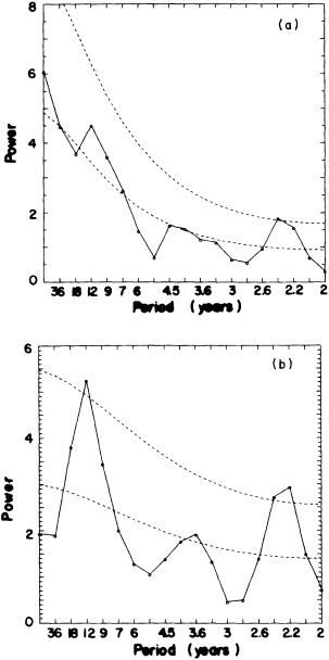
FIGURE 3
(a) Power spectrum of EOF 2 of SST. The thin dashed lines represent the background red-noise spectrum and its 95 percent confidence limit. (b) As in (a) but for EOF I of air temperature.
ture and E1 of SST (not shown) are red, reflecting the dominance of the long trends before and after World War II.
The similarity of the leading EOFs of the independently measured fields of surface air temperature and SST lends credence to the patterns.
We have examined the sensitivity of the leading EOF patterns of air temperature to temporal filtering. In view of the power spectrum of E1 of air temperature, we pre-filtered the data to emphasize (a) the biennial time scale and (b) the decadal time scale, and then computed EOFs. The first EOF of each of the sets of filtered data (not shown) is nearly identical to the first EOF based on unfiltered data. For the biennial time scale, the first EOF accounts for 26 percent of the variance; on the decadal time scale, it accounts for 29 percent. In view of the low-frequency behavior of E2 of air temperature, we computed EOFs based on lowpass filtered data (half-power point at 5 years). The first EOF of the low-pass filtered data (not shown), which resembles the second EOF of the unfiltered data, accounts for 29 percent of the variance of the low-pass filtered data. The correlation coefficient between the time series of E2 (unfiltered) and El (low-pass) is 0.88. Thus, although the first and second EOFs of unfiltered air temperature are not well separated according to the criterion of North et al. (1982)— they explain 21 percent and 17 percent of the variance, respectively—the sensitivity experiments described above suggest that they are distinct modes of variability.
RELATION OF SURFACE TEMPERATURE VARIABILITY TO THE SURFACE ATMOSPHERIC CIRCULATION
Dipole Pattern
How are the dominant modes of variability in surface temperature related to anomalies in the surface atmospheric circulation? Figure 4a shows the patterns of SST and surface wind anomalies regressed on the time series of E2 of SST (a similar picture is obtained if E1 air temperature is used in place of E2 SST). Note that the polarity of E2 SST is opposite from that shown in Figure 1c and that the SST pattern has been smoothed in space with a 3-point binomial filter. The relationship between the surface wind and SST anomalies is primarily local: stronger-than-normal westerlies and trade winds are coincident with cooler-than-normal temperatures, and southerly wind anomalies are associated with warmer-than-normal temperatures. The negative SST anomalies east of Newfoundland are located slightly upstream of the largest wind anomalies where the air-sea temperature differences are largest. The local nature of the wind/temperature relationships suggests that changes in the air-sea fluxes and wind-induced vertical mixing processes contribute to the formation of the SST anomalies. Ocean modeling experiments by Luksch et al. (1990) and Alexander (1990) confirm this interpretation. A somewhat surprising result is that the wind/temperature relationships are similar on decadal and biennial time scales (not shown).
Is the wind pattern shown in Figure 4a a preferred mode of variability in the atmosphere? Figure 4b shows the second combined EOF of sea level pressure and zonal wind, based on winter means for 1900 to 1989. This mode accounts for 15 percent of the variance in the combined fields. The meridional wind pattern was obtained by regressing the meridional wind anomalies on the time series of the com-
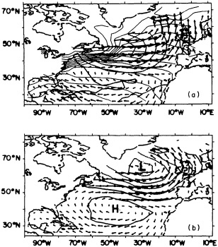
FIGURE 4
(a) SST (bold solid and dashed contours) and wind anomalies (arrows) regressed on the time series of EOF 2 SST. Also shown is the climatological SST distribution (thin contours). Note that EOF 2 of SST here has polarity opposite to that shown in Figure 1c; it has been smoothed in space with a 3-point binomial filter. (b) Combined EOF 2 of sea level pressure and zonal wind, based on winter means of 1900 to 1989. The meridional wind field was obtained by regressing meridional wind anomalies on the time series of the combined EOF. This mode explains 15 percent of the variance in the combined pressure and zonal wind fields.
bined EOF. The wind and pressure distributions in Figure 4b are consistent with the geostrophic relation, lending credence to the patterns. The wind patterns in Figures 4a and 4b are similar, indicating that E2 SST is coupled to a dominant mode of variability in the atmosphere. The power spectrum of the second combined EOF of pressure and zonal wind, shown in Figure 5, exhibits peaks at biennial and decadal time scales, similar to those found for E1 air temperature and E2 SST. The circulation mode represented by the combined EOF corresponds to the West Atlantic pattern as defined by Wallace and Gutzler (1981), although the northern center of action in the sea level pressure field is centered about 5° of longitude east of the corresponding feature in the West Atlantic pattern.
Time series of the various surface parameters to the east of Newfoundland (the center of actions of E1 air temperature and E2 SST) are presented in Figure 6. These records have been low-pass filtered with a 3-point binomial filter. Air temperature and SST were averaged over the region bounded by [52°-40°N, 50°-30°W]; zonal wind was aver-
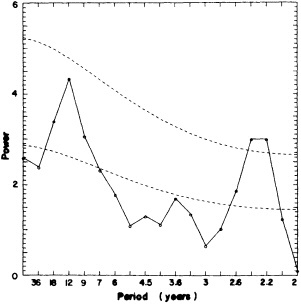
FIGURE 5
Power spectra as in Figure 3a, but for EOF 2 of the combined fields of sea level pressure and zonal wind.
aged over the region within [48°-38°N, 52°-22°W] and the geostrophic zonal wind was calculated from sea level pressure differences between [40°-32°N, 52°-22°W] and [52°-44°N, 52°-22°W]. Note that the air and sea temperatures and the winds and pressures were measured independently, so the comparisons provide a means of assessing data quality. All four parameters exhibit prominent decadal variability in the area east of Newfoundland; the amplitude of the decadal surface temperature (wind) fluctuations is a b o u t 1 . 5 ° C (1.5 m s-1). The correlation between the air temperature and SST time series is 0.88, and that between the measured and geostrophic wind series, 0.80. The high correlations attest to the reality of the decadal signal. The squared coherence between the SST and zonal wind time series (not shown) exceeds the 99 percent significance level at the decadal period, with a phase lag of 180° between the two parameters.
It is apparent from the time series in Figure 6 that the time scale of the quasi-decadal fluctuations was longer after about 1940 than it was before then. This is borne out by calculations of the power spectra for the pre- and post-1944 periods. During the period 1900 to 1944 the decadal spectral peak is centered at 9 years, whereas during 1945 to 1988 it is centered on 12 years (not shown). Thus, the decadal fluctuations are by no means regular.
Gulf Stream Pattern
The dominant features of the time series of El of SST and E2 of air temperature are the cold period of 1900 to 1929 and the warm period of 1939 to 1968 (Figures 1b and 2d). These cold and warm epochs may also be identified
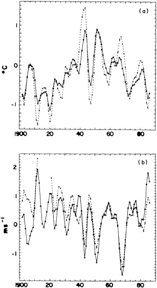
FIGURE 6
Time series of winter anomalies east of Newfoundland of (a) SST (solid) and surface air temperature (dashed) and (b) zonal wind (solid) and geostrophic zonal wind calculated from sea level pressure differences (dashed). All curves are smoothed with a 5-point binomial filter. See text for definition of indices.
on the basis of globally averaged temperatures (cf. Folland et al., 1984) and North Atlantic basin-averaged temperatures (cf. Bottomley et al., 1990). The surface temperature, wind, and sea level pressure differences between the warm and the cold period are shown in Figure 7. A minimum of 20 winters was required for the period average in each grid square. The surface wind and sea level pressure fields (Figure 7a) are dynamically consistent, with negative pressure anomalies along 40°N and easterly (westerly) wind anomalies to the north (south). The maximum sea level pressure difference is approximately 3 mb, and the largest wind-
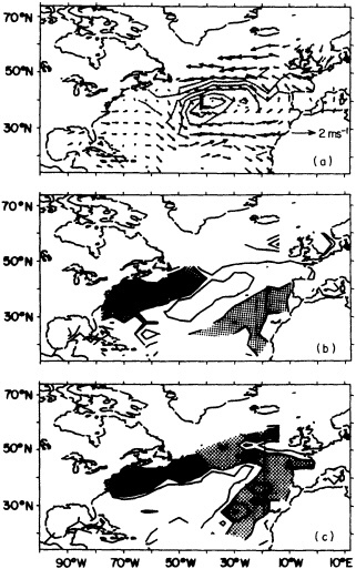
FIGURE 7
Difference between the periods 1939 to 1968 and 1900 to 1929 of winter (a) sea level pressure and surface wind, (b) SST, and (c) surface air temperature. In (a) the contour interval is 0.5 mb, with negative contours dashed. The lowest pressure anomaly is -3mb. Wind scale is indicated in lower right. In (b) light shading indicates values between 0.8°C and 1.0°C; heavy shading indicates values greater than 1.0°C. Contour interval is 0.2°C. In (c) light shading indicates values between 0.6ºC and 0.8°C; heavy shading indicates values greater than 0.8°C. Contour interval is 0.2°C.
speed anomaly is around 1.5 m s-1. This circulation pattern, which resembles the negative phase of the North Atlantic Oscillation (cf. Barnston and Livezey, 1987), represents an overall weakening of the basin-wide wind system.4 Similar
results were obtained by Parker and Folland (1988) from historical sea level pressure analyses. The SST (Figure 7b) and surface air temperature (Figure 7c) anomaly patterns are grossly similar: Both exhibit maximum positive anomalies (about 1°) along the Gulf Stream east of Cape Hatteras, and positive anomalies of smaller amplitude in the eastern ocean. There is some indication of a poleward amplification of the air-temperature anomalies, but the data are sparse north of about 55°. (Stations on Greenland, Iceland, and Scandinavia experienced a warming of approximately 2° during the 1920s and 1930s (Jones and Kelly, 1984).) Although the SST (and to a lesser extent the air-temperature) records suffer from discontinuities around World War II (cf. Jones et al., 1986c), the similarity between the air and sea temperature changes lends credence to the patterns in Figure 7. The ''corrected" SST data set of Bottomley et al. (1990) yields a similar pattern, although the warming along the Gulf Stream does not extend as far eastward as in the COADS (not shown).5
The wind/temperature relationships are different from those associated with the dipole pattern discussed above. While there is some evidence of wind anomalies overlying SST anomalies in the eastern portion of the basin, the largest surface-temperature anomalies occur in the west, upstream of the atmospheric-circulation anomalies. Whether the temperature anomalies along the Gulf Stream are connected with changes in the strength or position of the current is unknown. However, it is worth noting that a northward shift of the Gulf Stream of only 50 km would be sufficient to produce the observed warming. An alternative explanation for the warming along the Gulf Stream is a reduction in frequency or intensity of cold air outbreaks. This would occur if the temperatures over eastern North America were elevated or the offshore winds were reduced.
To examine the robustness of the patterns and to test whether the patterns are artifacts of data discontinuities around World War II, we computed the linear least-squares trends during the period 1917 to 1939. The data were first smoothed in time with a 3-point binomial filter to enhance the low-frequency signals. The surface wind and sea level pressure fields (Figure 8a) exhibit a cyclonic circulation trend in the central North Atlantic, similar to the results from the epoch analysis. Over the western North Atlantic, the trend analysis shows easterly wind anomalies, which are consistent with the pressure field, whereas the epoch analysis shows weak westerly anomalies. The trends in SST (Figure 8b) and air temperature (Figure 8c) are similar to the results from epoch analysis; the largest warming occurs
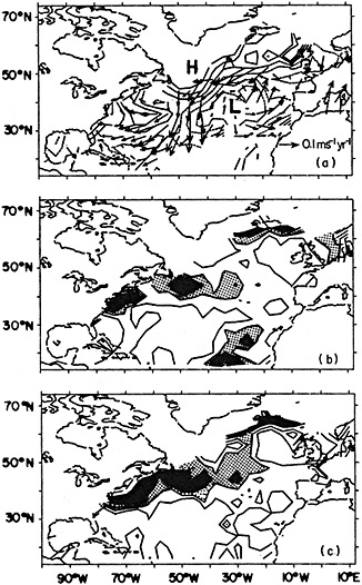
FIGURE 8
Linear least-squares trends during 1917 to 1939 of winter (a) sea level pressure and surface wind, (b) SST, and (c) surface air temperature. In (a) contour interval is 0.05 mb per year, with negative contours dashed. The wind scale is given in the lower right. In (b) and (c) the contour interval is 0.02°C yr-1. Light shading indicates values between 0.04°C yr-1 and 0.06°C yr-1; heavy shading indicates values greater than 0.06°C yr-1.
along the Gulf Stream, over the eastern subtropical Atlantic, and near Iceland. The warming along the Gulf Stream is not as continuous, and the warming in the eastern Atlantic not as pronounced, in the trend analysis as in the epoch analysis. As in the epoch analysis, the largest SST trends along the Gulf Stream occur remotely from the wind trends.
The time series of air temperature along the Gulf Stream [44°-36°N, 76°-42°W] and sea level pressure in the region bounded by [46°-34°N, 48°-20°W] and at Ponta Delgada, Azores [40°N, 28°W] are shown in Figure 9. Surface warming along the Gulf Stream occurred during the period 1920 to 1950 (amplitude about 2.5°C). Note that the temperatures
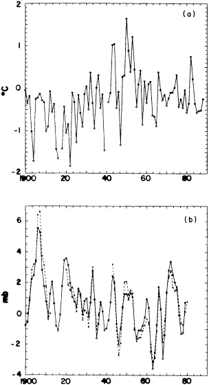
Figure 9
Time series of winter anomalies of (a) surface air temperature along the Gulf Stream [44°-36°N, 76°-42°W], and (b) sea level pressure in the central North Atlantic [46°-34°N, 48°- 20°W] and at Ponta Delgada, Azores [40°N, 28°W]. The curves in (b) are smoothed with a 3-point binomial filter. The solid (dotted) curve denotes pressures from Ponta Delgada (COADS).
since the mid-1950s have been relatively constant. The COADS and Ponta Delgada sea level pressure time series show remarkable agreement: Both indicate that the warming trend was accompanied by a decrease in the strength of the Subtropical High of approximately 4 mb. The pressure time series give the impression that the downward trend in the atmospheric circulation began about 1905 and lasted until 1962 or so, although the steepest continuous decline occurred during 1920 to 1940.
Bjerknes (1959) found a similar pattern of warming along the Gulf Stream during the first quarter of this century (he used differences between 1890 to 1897 and 1925 to 1932 to depict the warming trend). The warming was accompanied by a strengthening of the subtropical anticyclone, in contrast to the results of this study. We have attempted to reproduce the results of Bjerknes (1959) by using data from the COADS. While a warming along the Gulf Stream is hinted at in the COADS, it is much weaker than that depicted in Bjerknes (0.2°C versus 2°C; not shown). The pressure and wind patterns derived from the COADS broadly support Bjerknes's results.
DISCUSSION
One important mode of variability of the wintertime surface climate over the North Atlantic during this century is characterized by a dipole pattern in SSTs and surface air temperatures, with anomalies of one sign east of Newfoundland, and anomalies of the opposite polarity off the southeast coast of the United States. This pattern has been noted in the post-World War II data by Wallace et al. (1990), Cayan (1992b), and Kushnir (1994). Wind fluctuations occur locally over the regions of large surface-temperature anomalies, with stronger-than-normal winds overlying cooler-than-normal SSTs. The atmospheric-circulation anomalies resemble the West Atlantic pattern. This mode (both for surface temperatures and for surface winds) exhibits variability on quasi-biennial and -decadal time scales. The decadal fluctuations are irregular in length, averaging about 9 years before 1945 and around 12 years afterward. There does not appear to be any difference between the wind-SST relationships on the different time scales.
The local nature of the atmosphere-ocean relationships exhibited by the dipole pattern suggests that surface wind anomalies contribute to the formation of SST anomalies by altering the fluxes of latent and sensible heat at the ocean surface and the strength of vertical mixing in the upper ocean. Support for this interpretation is given by the ocean modeling studies of Alexander (1990) and Luksch et al. (1989).
Further research is needed to understand the origin of the quasi-decadal cycles in the North Atlantic ocean-atmosphere system. One possibility is that 90 years is not long enough to establish the significance of decadal cycles, and those that have occurred may be random in the sense that they are due to internal atmospheric processes. The decadal SST variations could then be interpreted as simply a reflection of low-frequency modulation of the high-frequency (synoptic and monthly) wind forcing. It should be noted that long (100-year) integrations of atmospheric GCMs, when subject to fixed SST boundary conditions, exhibit prominent low-frequency (decadal and longer) fluctuations (James and James, 1980; Feldstein, 1992).
A more inviting possibility is that the quasi-decadal time
scale is a property of the coupled ocean-atmosphere system. We note that decadal and longer time scale SST variations along the boundary between the sub-polar and sub-tropical ocean gyres are obtained in ocean GCMs as a result of self-sustained oscillations of the thermohaline circulation (cf. Weaver and Sarachik, 1991). In addition, atmospheric GCM experiments indicate that the local atmospheric response to an SST anomaly off Newfoundland is such that weak (strong) winds coincide with high (low) SSTs, reinforcing the original SST anomaly (Palmer and Sun, 1985; Lau and Nath, 1990). The implication of these studies is that observed mid-latitude climate anomalies may result from a positive feedback between the atmosphere and the ocean.
A third possibility is that the decadal atmospheric fluctuations are a response to decadal SST variations outside the North Atlantic. This scenario is difficult to test due to the lack of long marine records in the other ocean basins. Our preliminary results indicate that for the three most recent decadal oscillations, SSTs in the North Pacific are not coherent with those in the Atlantic.
One intriguing link we have found is that between sea ice in the Davis Strait-Labrador Sea region and quasi-decadal fluctuations. Figure 10a shows the time series of winter sea-ice concentration anomalies in the Davis Strait/Labrador Sea region from Agnew (1991), based on data from Walsh and Johnson (1979). The circles denote the winter (December-February) anomaly, plotted in the year in which January occurs. The solid curve shows the data smoothed with a 3-point binomial filter. Decadal variability is evident in the sea-ice record, with peaks occurring in the winters of 1957/ 1958, 1971/1972, and 1983/1984. Figure 10b shows the sea-ice record superimposed on the inverted time series of the second EOF of winter (November to March) SST (see Figure 1). Both the sea-ice and the SST time series have been detrended by subtracting least-squares parabolas based on the period 1950 to 1988, and smoothed with a 3-point binomial filter. It may be seen that the maxima in sea-ice concentration precede the minima in SST by one to two years. The correlation between the two time series is -0.26 with no lag, -0.62 when sea ice leads SST by 1 year, -0.76 when sea ice leads by 2 years, and -0.62 when sea ice leads by 3 years. The strong lag correlations indicate that, on the decadal time scale, winters of heavy sea ice in the Labrador Sea precede winters of colder-than-normal SSTs east of Newfoundland. It is plausible that the sea-ice anomalies in the Labrador Sea are advected southeastward, resulting in colder-than-normal SSTs east of Newfoundland the following (or second) year. Thus, the quasi-decadal cycle in SSTs east of Newfoundland may result in part from low-frequency Arctic sea-ice variations. Mysak and Manak (1989) and Mysak (1991) have also discussed the possible link between sea ice and SST anomalies in the northern North Atlantic, and Mysak et al. (1990) have postulated the existence of an interdecadal Arctic climate cycle involving
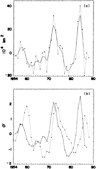
FIGURE 10
(a) Time series of winter sea-ice-area anomalies (104 km2) in the Davis Strait/Labrador Sea region from Agnew (1991), based on data from Walsh and Johnson (1979). The circles denote the winter (December to February) anomaly, plotted in the year in which January occurs. The solid curve shows the data smoothed with a 3-point binomial filter. (b) Sea-ice anomalies from (a) (solid curve) superimposed on the time series of EOF 2 of North Atlantic winter (November to March) SST (dashed curve). Note that the SST time series has been inverted. Both the sea-ice and SST time series have been smoothed with a 3-point binomial filter and detrended by subtracting a least-squares parabola based on the period 1950 to 1988.
runoff, sea ice, and SSTs. Further analysis is needed to elucidate the role of Arctic sea ice in decadal climate variability over the North Atlantic.
Another dominant mode of variability of the wintertime
surface climate over the North Atlantic during this century is associated with the global surface-warming trend during the 1920s and 1930s. The patterns of SST and air temperature change from 1900 to 1929 and from 1939 to 1968 (or, equivalently, the trends between 1917 and 1939) indicate that the warming was concentrated along the Gulf Stream east of Cape Hatteras. Warming also occurred over the Greenland Sea and the eastern subtropical Atlantic. The warming trend was accompanied by a decrease in the strength of the basin-scale atmospheric circulation (negative phase of the North Atlantic Oscillation). In marked contrast to the dipole EOF pattern, the wind changes occurred downstream of the largest SST anomalies. Hence the gradual surface warming along the Gulf Stream may have been a result of altered ocean currents rather than of local wind forcing.
A similar idea has been put forth to explain the cooling in the North Atlantic from the 1950s to the early 1970s (Levitus, 1989; Greatbach et al., 1991; Kushnir, 1994). The cooling trend was accompanied by a decrease in the transport of the Gulf Stream, as diagnosed from subsurface data by Greatbach et al. (1991). The decrease in Gulf Stream transport was in turn traced to bottom-pressure torque effects rather than wind effects (Greatbach et al., 1991).6
In a recent coupled atmosphere-ocean GCM experiment, Manabe and Stouffer (1988) showed that an intensified oceanic thermohaline circulation is associated with surface warming at high latitudes of the North Atlantic, and with an intensification and poleward shift of the Gulf Stream. The model's atmospheric response to an intensified thermohaline circulation is a weakening of the basin-wide wind system; this is consistent with the reduced baroclinicity. It is tempting to speculate that the climatic trends observed over the North Atlantic during the 1920s and 1930s were due to an intensification of the thermohaline circulation. However, we note that SSTs in the South Atlantic also warmed during this period (cf. Bottomley et al., 1990), contrary to the cooling observed in Manabe and Stouffer's experiment. Further modeling studies are needed to elucidate the role of the ocean circulation in low-frequency climate variability.
ACKNOWLEDGMENTS
We thank Ludmilla Matrosova for her help with the data processing. We are indebted to Harry van Loon for stimulating discussions and to Michael Alexander for his thoughtful review of the manuscript. James Hurrell kindly provided the Bottomley et al. (1990) data set. This work was supported by a grant from NOAA's Climate and Global Change Program.
|
6 |
It should be noted that the spatial pattern of cooling during the 1950s to 1970s was somewhat different from the pattern of warming during the 1920s and 1930s (see Kushnir, 1994). |
Commentary on the Paper of Deser and Blackmon
LAWRENCE A. MYSAK
McGill University
Dr. Deser presented a very nice study. I enjoyed it, but I do not have a lot of comments at this stage. Some postwar data sets that have been analyzed show two to three cycles of interdecadal variability in the empirical orthogonal functions, for example. In Dr. Deser's analyses we have now seen decadal-scale variability over a 90-year record, which I for one really appreciate.
I think it is important to emphasize that only the winter data was analyzed. Dr. Deser and I discussed earlier whether this decadal variability shows up in other seasons, such as summer, and thus is a year-round signal. I think the answer is that it is there in the summer, but it is not as strong. It is definitely much more intense in winter. I should perhaps mention here that winter is defined as being from November to March, a five-month period.
The two time scales that I found particularly fascinating in the paper were the decadal and the biennial. While I will not discuss the biennial any further here, I just want to point out some recent work of one of our Ph.D. students at McGill, J. Wang, who also noticed a quasi-biennial cycle in the ice cover in the Labrador Sea and the Baffin Bay region. In addition, he found quite a strong correlation between anomalies in sea-ice extent and the North Atlantic oscillation (which is defined as a winter index).
The decadal time scale Dr. Deser discusses clearly falls between two familiar time scales: the North Atlantic oscillation, which has a period of 7 to 8 years, and the interdecadal cycles in the Arctic, which I shall discuss in my own presentation. Also, many recent modeling studies of the thermohaline circulation in the North Atlantic have shown the existence of internal oscillations with decadal to interdecadal periods.
I should like to list some relevant references, which I believe were not mentioned in the paper. Also, I might remark that many of these papers are by various people at this workshop. One piece of work is the master's thesis
done in 1987 by Gordon Fleming at the Naval Postgraduate School. He was supervised by John Walsh, who is here. One of the interesting calculations in the thesis is the cross-correlation analysis of the COADS SST in the Labrador-Greenland-Barents Sea region and the position of the ice edge. Fleming found the two to be inversely correlated, not unlike Dr. Deser's findings for the Davis Strait. However, I believe Fleming was able to show that in some regions the SST actually leads the ice edge and therefore could be used as a predictor.
A recent paper by me and Manak (Atmosphere-Ocean, 1989) studying 32 years of sea-ice concentration data clearly showed the existence of a decadal oscillation of the sea-ice cover in the Labrador Sea and in the Barents Sea. The signal in the former region is the same as that shown in Dr. Deser's Figure 10a. In the Greenland Sea, variations in the sea-ice extent seemed to have a much longer time scale, because there the sea ice was dominated by a big ocean event during the 1960s and early 1970s that we have now associated with the Great Salinity Anomaly.
In that paper Manak and I suggested something that might set up an oscillation of 10 to 12 years, namely, the circuit time of the subpolar gyre in the northern North Atlantic. While 12 to 14 years was the circuit time for the GSA, there was nothing to reinforce it within the subpolar gyre region. Thus we abandoned the idea that there might be self-sustained oscillations of this period in this region.
Other papers by Mysak et al. (Climate Dynamics, 1990) and Marsden et al. (JGR, 1991) showed that salinity and sea-ice extent are highly correlated in the Greenland and Labrador seas, and that there is advection of both ice and salinity anomalies from the Greenland Sea into the Labrador Sea, with an advection time of a few years.
In terms of modeling studies, I first want to mention M. Ikeda (Atmosphere-Ocean, 1990), who developed an ocean model for the decadal oscillations in the Barents-Greenland seas. He emphasized that there were feedbacks between the atmosphere and the ocean in the Barents Sea. In 1991, Weaver and Sarachik published in Atmosphere-Ocean the first model evidence of a decadal oscillation in the thermohaline circulation in the North Atlantic. The physical location of the oscillation is somewhat further south than the Greenland-Labrador Sea, because it is centered between the subtropical and subpolar gyres. In more recent modeling studies with an improved geometry, Weaver and his coworkers have found that the decadal oscillation now extends to 20 years.
There has also been the more recent modeling work by Delworth and his colleagues at GFDL, who find a somewhat longer-time-scale fluctuation in the thermohaline circulation in a coupled atmosphere-ocean model. The period is 30 to 50 years, and the oscillation is found to have a dipole-like structure in the subsurface waters in the central North Atlantic. As for recent data studies looking at decade-to-century time scales, a paper in Climatic Change (Stocker and Mysak, 1992) presents a spectrum of the Koch ice index. (The Koch ice index is the number of weeks per year that ice affects the coast of Iceland.) A spectrum of 360 years of this index shows peaks at 90, 27, and 14 years.
Finally, a well-known time series of SST anomalies in the North Atlantic (45°N to 55ºN) is presented by Bryan and Stouffer in J. Marine Systems. This time series also shows interdecadal variability in the northwest Atlantic. In addition, in the Centre for Climate and Global Change Research's Report No. 91-1 (1991), I suggested that heavy ice conditions in the Greenland Sea lead cold SST anomalies in the northwest Atlantic (i.e., east of Newfoundland) by 4 or 5 years. Similarly, warm SST anomalies there were preceded by generally light ice conditions in the Greenland Sea during the previous 5 years.
Let me now refer you to two figures, Figures 10 and 12a in Stocker and Mysak. The first is a spectrum of the Koch ice index as defined above. During heavy ice conditions in the Greenland Sea, you have a high index; during mild conditions, a low index. This spectrum clearly shows a significant peak at 27 years, which indicates an interdecadal climate cycle in the northern North Atlantic. The second, a spectrum of the famous Central England temperature, shows peaks at around 15 and 7 years and an interdecadal peak at 24 years.
Discussion
NORTH: I wonder whether EOFs are the best way of describing the data. True, they are objective, but can you tell from analyzing them whether the Gulf Stream's temperature is changing or whether it is just shifting location?
DESER: If you look at the anomalies during the cold 30 years, or one of those decades, the warming first appears near Cape Hatteras. Then you see anomalies along the Gulf Stream east of Cape Hatteras, then east of Newfoundland, then in higher latitudes. A northward shift of about 50 km would be sufficient to produce the observed warming, and seems to me to be the simplest explanation.
MCWILLIAMS: The Gulf Stream warming pattern in your last figure is much broader than 50 km. While a mechanistic interpretation is tempting, an advective supply of heat from the Gulf Stream would be related to wind driving, whereas instead the forcing of the anti-cyclonic gyre is actually weakening.
GHIL: I just wanted to comment on the causes of the decadal variability. It seems to me that certain phase differences between fluctuation or oscillation are clear indications of coupling. A coupled atmosphere-ocean phenomenon seems the most plausible to me.
CAYAN: Have you looked at SST minus air temperature together with your Gulf Stream pattern? I wonder whether part of the reason for the change could be a change in the air mass distribution over the Gulf Stream. In extratropical regions the sensible flux is driven a lot by the temperature lapse rate, and to some extent by the wind.
DICKSON: I should like to show a slide, my Figure 14, that suggests two things. The first is that temperature and salinity show similar patterns, and I think were both involved, meaning that both the circulation and the ecosystem might have had large changes. The second is that the century-long trend covered a much larger area of the North Atlantic than we've been talking about—right up to the ice in the north, in fact.
Seasonal-to-Interannual Fluctuations in Surface Temperature over the Pacific: Effects of Monthly Winds and Heat Fluxes
DANIEL R. CAYAN1, ARTHUR J. MILLER1, TIM P. BARNETT1, NICHOLAS E. GRAHAM1, JACK N. RITCHIE1, AND JOSEF M. OBERHUBER2
ABSTRACT
Monthly heat fluxes and wind stresses are used to force the Oberhuber isopycnic ocean general-circulation (OPYC) model of the Pacific basin over a two-decade period from 1970 to 1988. The surface forcings are constructed from COADS marine observations via bulk formulae. Monthly anomalies of the fluxes and stresses are superimposed upon model climatological means of these variables, which were saved from a long spin-up. Two aspects of this work are highlighted, both aimed at a better understanding of the atmosphere-ocean variability and exchanges and at diagnosing the performance of the OPYC model in simulating monthly to decadal-scale variability. The first is the evaluation of the data used to force the model ocean, along with its relationship to other observed data. The second is the diagnosis of the processes revealed in the model that are associated with sea surface temperature (SST) variability, including their seasonal and geographic structure.
Although both random and systematic errors arise from the marine data and the bulk formulations, large signals in the air-sea fluxes are nonetheless consistent with the large-scale atmospheric circulation anomalies over the Pacific. This signal is large in a composite prepared from months with similar circulation modes. Also, latent and sensible heat-flux anomaly patterns correspond well to those of SST anomaly tendencies. Considering short-period variations, SST anomaly tendencies have typical magnitudes of 0.3°C mo-1. These are associated with monthly mean flux anomalies having typical magnitudes of 50 W m-2 and are consistent with observed mixed-layer depths. Decadal anomalies have much smaller magnitudes, perhaps reduced by two orders of magnitude, and it is here that the signal-to-noise problem is more severe. The forcing terms are generally products of variables, so realistic means and fluctuations of these variables are crucial for a successful simulation.
The 19-year simulation of the Pacific basin by the monthly marine data-forced OPYC model displays good skill in reproducing SST variability. These results represent the first
hindcast of which we are aware that uses both observed total heat-flux and wind-stress anomalies as forcing for such a long time interval. There is close agreement between the model SSTs and those observed in many regions of the Pacific, including the tropics and the northern extratropics. Besides performing credibly on the monthly time scale, the model captures the essence of low-frequency variability over the North Pacific, including aspects of a marked basin-wide change that occurred in 1976-1977. In the model's detailed heat budget, the anomalous air-sea heat fluxes, entrainment, and to a lesser extent horizontal advection, force thermal-anomaly changes in the mixed layer. Each of these components was apparently involved in the 1976-1977 decadal SST shift.
INTRODUCTION
Our purpose is to describe monthly to decadal variations in surface variability over the Pacific basin. The results presented combine a historical set of monthly marine observations and a two-decade numerical simulation (Miller et al., 1994a,b) that uses the Oberhuber (1993) isopycnic ocean general-circulation model.
The first part of the paper is an analysis of observed monthly surface marine atmospheric variability in relation to sea surface temperature (SST) over the Pacific Ocean. This observational evidence provides background to the second section of the paper, in which monthly wind stresses and heat fluxes are used to force an ocean general-circulation model (OGCM). In the observational section, we concentrate on the variability of the latent and sensible heat fluxes, since they provide a good example of the characteristics and problems involved in bulk formulations using the marine data. The fluxes exhibit monthly variability with large-scale organization, and their effect on the ocean can be detected in the monthly fluctuations of the SST anomaly field.
The second part of the paper reports on applying the marine data parameterizations to a simulation over two decades (1970-1988) of the Pacific Ocean basin using the OPYC OGCM. This run is forced by monthly mean wind stress and fluxes derived from surface marine observations, which are introduced in the first section. In assessing this run, we compare the model SST anomalies with observations, particularly their low-frequency variability. Further insight is provided by the model upper-ocean heat budget, which is not well described by observations.
Aside from diagnosing mechanisms causing monthly SST variability, one motivation for this simulation was to better understand a strong regime-like change in SST that occurred in the North Pacific basin during the mid-1970s (Douglas et al., 1982; Nitta and Yamada, 1989; Trenberth, 1990; Miller et al., 1994a,b; Graham, 1994; Trenberth and Hurrell, 1995, in this volume). Although thorough observational documentation of decadal-scale variability is lacking, glimpses from recent historical episodes suggest that this "gray area" (Karl, 1988) of the variability spectrum contains important climate effects. The actual shift was identified in fall and winter of 1976-1977 when SSTs in the central North Pacific cooled markedly and SSTs along the west coast of North America warmed (Venrick et al., 1987; Trenberth, 1990; Ebbesmeyer et al., 1991). In the atmosphere, the shift involved a basin-scale deepening of the wintertime Aleutian Low System, and appears to have been at least partially instigated by forcing from the tropical Pacific (Graham, 1994; Trenberth, 1995, in this volume), although an alternative theory involves sea-air feedback and advection of thermal anomalies by the North Pacific subtropical gyre (Latif and Barnett, 1994). Accompanying changes in many other physical and biological variables in the North Pacific basin and around its margin were also noted (Venrick et al., 1987; Ebbesmeyer et al., 1991).
The bulk formulae parameterized heat fluxes, calculated from standard marine surface meteorological observations, are the only means of estimating a multi-year time history of the heat exchange over broad regions of the oceans. Similarly, SST has been measured routinely by merchant ships for several decades, and, in the absence of a comprehensive temperature-versus-depth set in the upper ocean, SST is used to infer the variability of the upper-ocean heat content. Although the ocean heat-content structure can be complex, during winter in the extratropics the upper ocean is quite well mixed and SST is a good indicator (White and Walker, 1974).
As is brought out in the section below, there is a rich variability, superimposed upon the climatological mean, that involves both atmospheric and oceanic fluctuations. Three tests of the surface heat budget are discussed here. The first two, which study the data directly, are to relate monthly anomalies of the latent and sensible fluxes to the anomalous atmospheric circulation and to anomalous tendencies of the SST field. The third is to incorporate the monthly bulk-formula wind stress and heat flux as forcing of an extended OGCM run and to compare the simulated versus the observed SST fields. These results represent the first hindcast of which we are aware that uses both observed total-heat-flux and wind-stress anomalies as forcing for such a long time interval.
OBSERVATIONAL EVIDENCE FOR ANOMALOUS AIR-SEA HEAT EXCHANGE
Data
The primary data employed in the observational section of this study, as well as in the model forcing, are gridded
monthly mean ship-observed marine surface data for 1946-1986 from the Comprehensive Ocean-Atmosphere Data Set (COADS) (Slutz et al., 1985; Woodruff et al., 1987). From this set, several variables are employed, including the scalar wind or wind speed w, west-to-east and south-to-north horizontal surface wind components u,v, sea level pressure (SLP), specific humidity qa, air temperature T, and sea surface temperature SST. Derived variables include the products {w?T}, {w?q}, {wu}, and {wv}, where the monthly averages of products of the individual observations are indicated by { }. These products are involved in parameterizing the sensible and latent heat flux, and the horizontal wind-stress components, respectively.
To reduce errors in the data fields and condense the number of data in the analyses, the COADS 2°-gridded "Monthly Summaries Trimmed" data were averaged onto 5° squares, centered at 5° latitude-longitude intersections. This averaging was applied to the anomalies of the 2° squares, rather than their values, to avoid spurious 5° anomalies caused by poor sampling within the domain. Long-term means employed were calculated over 1950 to 1979. Details are provided in four papers by Cayan (1990; 1991, hereafter designated DC1; 1992a, designated DC2; and 1992b, designated DC3).
Bulk Formula Parameterizations
Latent and sensible heat exchange at the ocean surface is an important mechanism for venting ocean heat absorbed from solar radiation to the atmosphere. Globally, approximately 60 percent of the solar radiation absorbed at the earth's surface is released by latent and sensible heating, primarily from the ocean (Sellers, 1965). Gill and Niiler (1973) invoked scaling arguments in the governing equations to infer that, over large scales (= 1000 km meridionally and = 3000 km zonally), anomalous open-ocean surface temperature changes are dominated by changes in heat fluxes through the surface, rather than by advective influences. Since they depend on both oceanic and atmospheric conditions, the latent and sensible fluxes vary strongly over space and time. In the extratropics, latent and sensible fluxes are greatest in fall and winter when the near-surface vertical gradients of humidity and temperature are largest and wind speeds are highest (Esbensen and Kushnir, 1981; Isemer and Hasse, 1985, 1987).
The bulk aerodynamic formulae used for the latent and sensible heat fluxes are
and
where Ql is the latent flux, Qs is the sensible flux, L is the latent heat of evaporation of water, and cp is the specific heat of air at constant pressure. Again, w is the wind speed, ?q is sea surface saturation minus air specific humidity, and ?T is SST minus air temperature. CE and CH are the transfer coefficients for latent heat and sensible heat, respectively, and are taken to be the modified Bunker coefficients given by Isemer and Hasse (1987). Unlike their mean values (Blanc, 1985), the anomalies of the fluxes are not particularly sensitive to the choice of exchange coefficients. A comparison of monthly anomalies obtained with these exchange coefficients to those from two other schemes yielded strong agreement (DC2).
The sense of the latent and sensible fluxes adopted throughout the paper is positive for heat entering the ocean from the atmosphere.
Errors in the Latent and Sensible Fluxes
Because of uncertainties in the bulk formulae and because the marine data have inaccuracies and are non-uniformly measured, the parameterized flux estimates contain errors. Although it is not possible to determine precisely the spatial and temporal characteristics of errors in the bulk-formulae-derived heat fluxes, estimates of their magnitudes have been attempted. In many regions the aggregate of the errors in the fluxes considerably exceeds the 10 W m-2 tolerance that has been targeted for climate studies (Taylor, 1984). Nevertheless, it will be shown that important climate variability (monthly to decadal time scales) is still contained in the flux estimates. A review of individual monthly maps of the fluxes finds that several have anomalies with magnitudes of 50 W m-2 or greater, a "signal" which is well beyond reasonable error estimates. From our observational and modeling experience, the character of this error, as much as its magnitude, is crucial. For example, a 10 W m-2 error is probably acceptable if it has a high-frequency, random variability, but it is intolerable if it has low-frequency (decadal-scale) changes.
Both random and systematic errors in marine observations and errors in the bulk formulae contaminate the monthly mean fluxes (Weare, 1989; Taylor, 1984; DC1). Random measurement errors and errors from incomplete sampling of the natural weather fluctuations are reduced by averaging several observations together. Because the mean of the fluxes was removed and the resulting anomalies are generally only a fraction of the mean, the non-time-varying biases are reduced considerably. The largest random errors in the flux estimates appear to be caused by sampling variability, and to a lesser extent by observation errors (DC1). This error was estimated by a Monte Carlo sampling exercise (DC1) where the mix of observations entering particular flux estimates within well-sampled regions was repeatedly re-sampled. The uncertainty of the monthly mean for well-sampled 5° squares (50 or more independent samples per month) is reduced to approximately 40 W m-2 or less for
the latent flux and to 20 W m−2 or less for the sensible flux. The density of observations is relatively high over the extratropics of the North Pacific and North Atlantic, with many 5°squares having 100 or more observations per month. However, the density is marginal-to-poor over the tropics and in the Southern Hemisphere, with fewer than 20 observations per month at many 5° squares. In these sparsely sampled regions, random errors in the monthly flux estimates are likely to be substantial. Consequently, in forcing the OGCM in the region between 20°N and 20°S and data-poor regions south of 20°S, we have resorted to a Newtonian damping scheme for the net flux anomalies.
Systematic errors are caused by biases in the bulk formulae and in the observations, and are not automatically reduced by averaging. Time-varying biases in the fundamental observations caused by changes in instrumental practices are probably a significant source of error. These errors are difficult to quantify, but the marine data have "global" (over the available COADS-covered region) trends in w and ΔT, which translate to changes of approximately 0.8 m s−1 and −0.2°C over 1950 to 1986. Because these seem to be at least partially caused by instrument and calibration changes over the period, the fluxes were adjusted to remove the effects of the global average linear trends. This adjustment reduced the linear change in the latent and sensible fluxes over 1950 to 1986 by about 20 W m−2 and 5 W m−2, respectively (DC1 and DC2). This adjustment has only minor influence on the high-frequency variability, but it does significantly affect the multi-year numerical model run, because the effects are cumulative. More discussion of the systematic errors in the marine data is provided below.
Anomalous Variability of the Heat-Flux Components
The dependence of the flux anomalies on the mean conditions and the anomalies of the fundamental surface variables was explored in DC1. For the monthly latent flux anomaly
where an overmark indicates the long-term monthly mean and a prime indicates the monthly anomaly. For monthly means, most of the variation comes from w and Δq, not from the exchange coefficients (DC1). The last term on the right-hand side of (3) does not contribute strongly to latent flux anomalies, because w and Δq monthly anomalies are not locally well correlated over most of the oceans (DC1). A similar relationship involving ΔT instead of Δq describes the monthly sensible flux anomalies.
Equation (3) shows that the joint behavior of mean values and anomalies of wind speed w, the ocean-surface saturation humidity-air humidity difference Δq, and the sea-air temperature difference ΔT must be included to determine the flux anomalies. For atmosphere-ocean models, this interplay between the mean and anomaly components is a challenge. It is not enough to simulate anomalies of w, Δq, and ΔT; their mean fields must also be properly represented.
There are strong seasonal and geographical modulations of the flux anomalies. In the extratropics the variance is greatest in fall and winter when w, Δq, and ΔT have largest mean values and strongest variability. The largest contributions to the extratropical variance of Q1 anomalies involve ![]() . Anomalies of Qs become important north of about 35°N, where their variance is dominated by the term involving
. Anomalies of Qs become important north of about 35°N, where their variance is dominated by the term involving ![]() . In the extratropics, the variance of each of these components is maximum along the western side of the basin, because strong ocean boundary currents and large air-mass differences between the upwind land mass and the sea cause great contrasts. Latent flux anomalies in the tropics often involve greater contributions from
. In the extratropics, the variance of each of these components is maximum along the western side of the basin, because strong ocean boundary currents and large air-mass differences between the upwind land mass and the sea cause great contrasts. Latent flux anomalies in the tropics often involve greater contributions from ![]() than do those in mid-latitudes, although the eastern tropical Pacific has relatively large contributions from
than do those in mid-latitudes, although the eastern tropical Pacific has relatively large contributions from ![]() .
.
The Δq and ΔT monthly anomalies are correlated (cooler air is usually drier), especially in the extratropics, so the latent and sensible anomalies usually reinforce each other, yielding relatively large net heating anomalies. In the extratropics, flux anomalies are linked to the local wind direction, but in the tropics they are usually not (DC2). North of about 15°N, the largest positive anomalies are associated with northerly to northwesterly winds; they probably result from meridional advection of atmospheric humidity and temperature, and also from changes in the strength of the westerly winds. In the tropics, there is little relationship between wind direction and the flux anomalies, since horizontal gradients of humidity and temperature are weak and the wind direction is relatively steady.
How does the variability of the anomalous latent and sensible fluxes compare with that of the radiative fluxes? The balance of the heat-flux anomaly terms is distinctly different from that of the mean terms. Combined anomalies of Ql and Qs often exceed 50 W m−2 over regions several hundred kilometers in extent (DC1 , DC2, and DC3). These estimates indicate that monthly anomalies of Ql and Qs are usually larger than those of the radiative components. Comparing the variances of Ql and Qs, with those of bulk-formulae-estimated net solar radiative flux QSW and infrared flux QIR, DC1 found that: (1) Ql and Qs, anomalies dominate the monthly anomalous surface heat budget during winter in the extratropics north of 30°N, (2) Ql anomalies dominate from about 15°N to about 30°N, and (3) Ql and QSW anomalies are about equally large from 15°N to 15°S.
Flux Anomalies and Atmospheric Circulation
Ql and Qs anomalies have regional-to-basin-scale coherence both the North Atlantic and North Pacific. The first four empirical orthogonal functions (EOFs) of the sum of the Ql and Qs anomalies (Q'l+s) account for about half of the total variance of this field in each basin (DC1). That these
patterns relate to the anomalous atmospheric circulation is evidence for a realistic flux-anomaly signal. The dominant atmospheric-circulation anomaly modes in the North Atlantic and North Pacific, represented as EOFs of the sea level pressure, produce systematic flux-anomaly patterns (DC2). The first SLP EOF in the North Pacific features a large pressure anomaly in the central North Pacific, and is associated with the well-known ''Pacific-North American" (PNA) pattern. Three correlation fields linking the PNA to surface variables are shown in Figure 1: the correlations between winter-month PNA time amplitudes and gridded fields of w (wind speed), Δq, and Ql+s anomalies. This set of maps, and others in DC2, show that the anomaly fields of w, Δq, and latent-plus-sensible flux are remarkably consistent with major SLP anomaly patterns over the North Pacific and North Atlantic. Negative SLP anomalies favor positive w anomalies to their south and negative w anomalies to their north, associated with shifts in storm tracks and changes in the mean wind field. Negative SLP anomalies favor positive Δq (and ΔT) to their west, and negative Δq to their east, probably because of meridional advection of air temperature and humidity. The flux anomalies are a hybrid of these patterns, with enhanced sea-to-air fluxes to the southwest and diminished fluxes to the east of negative SLP anomalies.
For the strong Aleutian low phase of the PNA, the anomalous wind-speed field is dominated by a single zonally oriented high-wind patch to the south of the Low in the central North Pacific, with out-of-phase tendencies to the north and the south. Δq and ΔT anomalies are arranged in pockets to the southwest (positive anomalies) and to the east (negative anomalies) of the low. Farther afield, a positive anomaly center appears in the Gulf of Mexico, reflecting the well-known downstream teleconnection of deep troughs and cold dry air outbreaks leading to positive ΔT and Δq anomalies over the southeast United States. The pattern has a broad center of positive anomalies to the southwest of the Aleutian Low, and a region of negative anomalies east of the Low along the West Coast. In the section of this paper that reports on the ocean model, it is shown that low-frequency changes in the PNA between the 1960s and 1980s were associated with marked variations in heat flux and wind stress, which produced striking variability in the upper-ocean thermal structure.
Flux Anomalies and SST
Does the heat flux drive the SST, or does the SST drive the heat flux? The relationship between SST and the climatological mean of total latent and sensible heat flux appears to support two different points of view. On one hand, the fluxes may be driven by the SST: High ocean-to-atmosphere fluxes are found in the tropics where there is warm water and high saturation-vapor pressure, and low fluxes occur
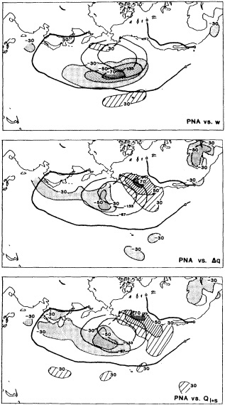
FIGURE 1
The correlation coefficients (× 100) between time series of the amplitudes of Pacific-North American EOF and our all-grid-point time series of w' (above), Δq' (middle), and Q'l+s, (below) in the North Pacific for the winter months, 1950-1986. Solid contours show PNA pattern. Significant correlation regions are superimposed upon the EOF patterns; shading indicates regions where the magnitude of the correlation is ≥0.3. Significant positive/negative correlations are shown by stippling, hatching in upper two frames; and by hatching, stippling in lower frame.
in high latitudes and along the eastern side of the ocean basins where surface temperatures are cool. Concerning the anomaly relationships, there is evidence for the SST-forcing-flux mechanism in the warm-season extratropics and in the tropics (Cayan, 1990; Liu and Gautier, 1990).
On the other hand, in the extratropics the fluxes appear
to force the temperature (Gill and Niiler, 1973; DC3): SST is coolest in late winter following the highest ocean-to-atmosphere fluxes. For the flux-forcing-SST case to be valid, the SST anomaly must play a negligible role in determining the flux, so that the flux is driven by atmospheric conditions—i.e., w, Ta, and q variations dominate the variations of SST. Indirectly, this scenario has been investigated by relating SST anomalies to the large-scale atmospheric circulation (Namias, 1972; Davis, 1976; Wallace et al., 1990). While all of these studies established a definite connection between the monthly or seasonal mean circulation and the SST anomalies, they could only infer the role of anomalous heat flux in forcing SST anomalies. When atmospheric fields are related to contemporaneous monthly SST anomalies, it is difficult to determine whether SST is forcing the atmosphere, both fields are being forced by some other agent, or the atmosphere is forcing the SST.
In testing the phase relationship between anomalies of the estimated flux and SST, the dominant linkage exhibited in the extratropics is that the latent and sensible flux anomalies force the SST anomalies, rather than SST anomalies' forcing the flux anomalies (DC3). Historical time series of flux data provide the basis for directly testing the forcing. Correlations between bulk formulae fluxes and anomalous temperature variations have been documented over the North Pacific by Clark et al. (1974) and Frankignoul and Reynolds (1983), and in the western tropical Pacific by Meyers et al. (1986). As was reported in DC3, the latent and sensible heat-flux anomalies proved to strongly affect monthly changes in SST anomalies over a large portion of the world oceans, in particular the North Atlantic and the North Pacific. A simple thermodynamic model was adopted to relate the flux anomalies to the tendency (time rate of change) of the SST anomalies. More discussion of the full mixed-layer thermodynamic equation is given below, and a comprehensive treatment is provided by Frankignoul (1985). Note that the temperature equation predicts the tendency of the SST anomaly ![]() , not the anomaly itself; the tendency is represented here by its finite-difference forms,
, not the anomaly itself; the tendency is represented here by its finite-difference forms, ![]() . The flux parameterizations do not contain knowledge of the SST tendency, so the relationship of fluxes to SST-tendency anomalies is an independent test of the influence of the fluxes.
. The flux parameterizations do not contain knowledge of the SST tendency, so the relationship of fluxes to SST-tendency anomalies is an independent test of the influence of the fluxes.
Having a higher-frequency character than the anomaly itself, ![]() has nearly as many independent samples of
has nearly as many independent samples of ![]() as there are months; four decades of records contain approximately 120 independent December-January-February samples.
as there are months; four decades of records contain approximately 120 independent December-January-February samples.
Spatial Distribution of Flux versus SST Tendency Anomalies
The geographical distribution of the correlations between Q'l+s and ![]() observations for winter months is examined in Figure 2. The 0.3 level is used as a threshold of statistical significance. Meaningful correlations on this map are almost everywhere positive, as they were for zonal averages of the two fields (DC3). Strongest correlations (= 0.5) are found mostly between about 25°N and 40°N within the anticyclonic subtropical gyres of the two oceans. For the North Pacific, strongest correlations are east of 180° and extend to the California Current. Though significant in many locations, correlations are weaker in the western North Pacific and from the tropics to 30°S. In the central North Atlantic, the flux and
observations for winter months is examined in Figure 2. The 0.3 level is used as a threshold of statistical significance. Meaningful correlations on this map are almost everywhere positive, as they were for zonal averages of the two fields (DC3). Strongest correlations (= 0.5) are found mostly between about 25°N and 40°N within the anticyclonic subtropical gyres of the two oceans. For the North Pacific, strongest correlations are east of 180° and extend to the California Current. Though significant in many locations, correlations are weaker in the western North Pacific and from the tropics to 30°S. In the central North Atlantic, the flux and ![]() anomalies have strong correlations in the central subtropical gyre as well as in the high-variance western North Atlantic region. Seasonally, most of the regions have strongest correlations in winter.
anomalies have strong correlations in the central subtropical gyre as well as in the high-variance western North Atlantic region. Seasonally, most of the regions have strongest correlations in winter.
Near the equator between 5°N and 5°S in all three basins, Q'l+s and ![]() are not well correlated. Correlations between zonal average flux and SST anomalies (DC3; not shown) indicate that in the tropics, the flux and SST anomalies (not the tendencies) tend to be negatively correlated. This suggests that the flux is driven by SST, presumably because equatorial SST anomalies are governed more by internal ocean processes than by the air-sea heat exchange.
are not well correlated. Correlations between zonal average flux and SST anomalies (DC3; not shown) indicate that in the tropics, the flux and SST anomalies (not the tendencies) tend to be negatively correlated. This suggests that the flux is driven by SST, presumably because equatorial SST anomalies are governed more by internal ocean processes than by the air-sea heat exchange.
![]() versus Fluxes during Strong Atmospheric-Circulation Modes
versus Fluxes during Strong Atmospheric-Circulation Modes
The organization of the latent-plus-sensible flux anomalies (Q'l+s) by the anomalous atmospheric circulation can be used to test the consistency of large-scale links between the flux and SST tendency anomalies ![]() . If the SST tendency anomalies are caused by the fluxes, they should have corresponding patterns. In DC3, the organization by the circulation was exploited by using the dominant SLP EOF modes as an index to compare flux-anomaly and corresponding SST-anomaly tendency patterns.
. If the SST tendency anomalies are caused by the fluxes, they should have corresponding patterns. In DC3, the organization by the circulation was exploited by using the dominant SLP EOF modes as an index to compare flux-anomaly and corresponding SST-anomaly tendency patterns.
To identify strong winter-circulation months, extreme positive and negative EOF amplitudes were chosen for each SLP EOF (DC2 and DC3). Using this criteria, several (10-30) months of each of the extreme EOF modes (positive and negative amplitudes) were selected. Composites of Q'l+s and ![]() were formed by averaging the fields during the respective extreme months. For brevity, the composites were expressed as the difference between averages of positive (strong) and negative (weak) phase months of the SLP EOFs.
were formed by averaging the fields during the respective extreme months. For brevity, the composites were expressed as the difference between averages of positive (strong) and negative (weak) phase months of the SLP EOFs.
In both northern oceans, the patterns of ![]() are well aligned with the flux anomaly patterns. In the North Pacific, composite
are well aligned with the flux anomaly patterns. In the North Pacific, composite ![]() differences and Q'l+s differences corresponding to positive-minus-negative extremes of the PNA pattern are shown in Figure 3. Remarkably, the flux and
differences and Q'l+s differences corresponding to positive-minus-negative extremes of the PNA pattern are shown in Figure 3. Remarkably, the flux and ![]() signatures of the PNA are marked out more than halfway around the hemisphere. Major centers of
signatures of the PNA are marked out more than halfway around the hemisphere. Major centers of ![]() are closely matched to those of Q'l+s, which confirms that
are closely matched to those of Q'l+s, which confirms that
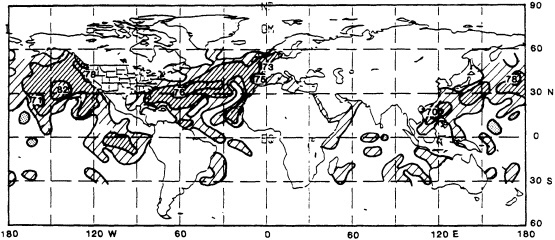
FIGURE 2
Correlation coefficients (×100), mapped for global ocean Q'l+s vs. ![]() at each grid point, for the winter months, 1946-1986. Contours at 0.3, 0.5, and 0.7. Light and heavy shadings indicate correlations =0.3 and =0.5.
at each grid point, for the winter months, 1946-1986. Contours at 0.3, 0.5, and 0.7. Light and heavy shadings indicate correlations =0.3 and =0.5.
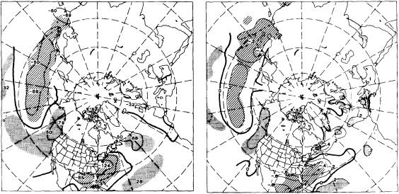
FIGURE 3
Difference of composites of Q'l+s (W m-2; left) and ![]() (°C mo-1; right) associated with positive (deep Aleutian Low phase) vs. negative extremes of EOF I of North Pacific SLP. Shading indicates regions where the difference exceeds the 95 percent confidence limit using a two-tailed t-test.
(°C mo-1; right) associated with positive (deep Aleutian Low phase) vs. negative extremes of EOF I of North Pacific SLP. Shading indicates regions where the difference exceeds the 95 percent confidence limit using a two-tailed t-test.
they are causally linked. At the centers, ![]() differences exhibit magnitudes of 0.2°C mo-1 to 0.8°C mo-1. Corresponding flux differences range from about 30 to 120 W m–2 Over the North Pacific, the PNA incorporates a swath of positive Q'l+s differences across mid-latitudes (centered at 40°N) from Asia to 140°W, and an arc of negative Q'l+s differences extending from the subtropics at 20°N, 160°E to the eastern North Pacific border, from California to the Gulf of Alaska. Downstream, the strong downstream arm of the PNA produces negative Q'l+s differences in the Gulf of Mexico and the eastern seaboard of the United States, and positive anomalies in the subtropical North Atlantic (20°N, 50°W) and east of Newfoundland. Throughout the North Pacific and North Atlantic, the PNA-associated
differences exhibit magnitudes of 0.2°C mo-1 to 0.8°C mo-1. Corresponding flux differences range from about 30 to 120 W m–2 Over the North Pacific, the PNA incorporates a swath of positive Q'l+s differences across mid-latitudes (centered at 40°N) from Asia to 140°W, and an arc of negative Q'l+s differences extending from the subtropics at 20°N, 160°E to the eastern North Pacific border, from California to the Gulf of Alaska. Downstream, the strong downstream arm of the PNA produces negative Q'l+s differences in the Gulf of Mexico and the eastern seaboard of the United States, and positive anomalies in the subtropical North Atlantic (20°N, 50°W) and east of Newfoundland. Throughout the North Pacific and North Atlantic, the PNA-associated ![]() differences mirror the flux differences, having centers co-located with the flux differences. Magnitudes of the corresponding flux and SST anomaly tendencies are consistent with typical observed mixed-layer depths, approximately 100 to 250 m in winter and 10 to 40 m in summer. Similar seasonal behavior and the relation between the flux and SST tendency are replicated in the OGCM, as presented in the following section.
differences mirror the flux differences, having centers co-located with the flux differences. Magnitudes of the corresponding flux and SST anomaly tendencies are consistent with typical observed mixed-layer depths, approximately 100 to 250 m in winter and 10 to 40 m in summer. Similar seasonal behavior and the relation between the flux and SST tendency are replicated in the OGCM, as presented in the following section.
OCEAN MODEL
In this section, we report on an extended run of the OPYC OGCM, which was forced by the wind stress and fluxes derived from the surface marine observations (see Miller et al., 1994a,b). The OPYC model, developed by Oberhuber (1993), consists of eight isopycnal interior ocean layers fully coupled to a surface bulk mixed-layer model, the latter also including a sea-ice model. The interior layers (fixed potential density) and the mixed layer (variable density) have prognostic thicknesses that vary as a function of space and time; the interior layers may have zero thickness, and the mixed layer has a minimum thickness of 5 m. The interior potential densities are specified in such a way as to yield increased vertical resolution (thinner layers) in the thermocline and less in the deep ocean (thick layers). The low horizontal resolution perforce disallows mesoscale eddy variability, which is probably unimportant in the evolution of large-scale SST anomalies. The ocean model solves the full primitive equations for mass, velocity, temperature, and salt for each layer in spherical geometry with a realistic equation of state. The domain is the Pacific Ocean from 70°S to 65°N and 120°E to 60°W. The grid resolution is 77 by 67 points. Resolution is enhanced near the equator and near the eastern and western boundaries. Open-ocean resolution in the middle latitudes is 4°, which is suitable for examining the large-scale variability. The conditions on horizontal solid boundaries are no-slip for velocity and thermally insulating for temperature. The model's Antarctic Circumpolar Current, however, has periodic boundary conditions and unrealistically connects to itself from 60°W to 120°E (half the global circumference). The surface boundary conditions for interior flow are determined by the bulk mixed-layer model, which is forced by the atmosphere. Frictional drag acts between each layer but most strongly along the bottom boundary, which has realistic topography. Horizontal Laplacian friction and diffusion with variable coefficients are also included.
A full discussion of the dynamics is given by Oberhuber (1993), who used the model in Atlantic Ocean modeling studies, and by Miller et al. (1992, designated MOGB below), who used an earlier version of this model for tropical Pacific Ocean circulation studies. Besides the differences in geometry and the forcing functions to be described, the present model differs from MOGB in the following ways: A horizontal finite-differencing scheme based on Bleck and Boudra (1981) that conserves both enstrophy and potential vorticity is implemented in this version of the model. In addition, for a more realistic mixed-layer depth (MLD) in the middle latitudes, the mean turbulent kinetic energy (TKE) input into the mixed-layer equation for entrainment velocity has been altered to provide for month-to-month variability, and is lower than that of the MOGB model. The net result is to reduce the MLD in the middle and high latitudes of the North Pacific relative to that of MOGB, with the present values being more typical of those observed.
Concerning the OPYC ocean general-circulation model, it is important to point out some potential defects that may obscure our interpretations (Miller et al., 1994a). First, horizontal advection may be underestimated because the model SST climatology is too weak, especially in the Northwest Pacific. Second, the Kuroshio is not well resolved, so the model cannot generate strong western boundary currents. This will impair its ability to advect SST anomalies to nearby open ocean regions. Third, a warm bias in the model winter SST field (approximately 4°C too warm) in the northern North Pacific results in an overly stable stratification that diminishes the effects of entrainment. Last, salinity variations were not included, and these may be important, particularly in high latitudes. Although the OPYC OGCM's rather low resolution has excluded the effects of oceanic mesoscale variability on SST anomaly generation, we expect that such anomalies would have spatial scales too small to provoke important reactions in the large-scale atmospheric fields (Klein and Hua, 1988; Halliwell and Cornillon, 1989; Miller, 1992).
Forcing Functions and Model Runs
Since no ocean model is perfectly realistic, any model forced by observed total heat fluxes (without any feedback) will establish an oceanic temperature climatology that will depart from the real observations. To circumvent this problem, we forced the model with observed anomalies of heat fluxes superimposed upon the model climatology rather than with the total observed flux fields. This scheme preserves the model ocean climatology, as follows. We first establish the model climatology by forcing with observed monthly long-term mean wind stresses, TKE input, and total heat fluxes derived from bulk formulae using monthly long-term mean atmospheric observations combined with model ocean temperature. After the oceanic system has reached an acceptably equilibrated state (gauged by the absence of drift in mean SST and MLD), monthly means of pertinent fields are saved for use in the later experiments.
Using the same strategy as that just discussed, the oceanic salinity field is stabilized to climatological average observations. However, the equilibrium salinity is very sensitive to the evaporation-minus-precipitation (E - P) field, which is not available at present from observations. Hence, we use Newtonian relaxation to the observed annual mean surface salinity field compiled by Levitus (1982) rather than attempting to specify E - P.
Spin-up
During a 35-year-long spin-up period, the model was forced by monthly long-term mean fields of atmospheric
wind stress, interpolated from analyses made by the European Centre for Medium-range Weather Forecasting (ECMWF), and total surface heat fluxes (latent, sensible long-wave radiation, and insolation), derived from bulk formulae using model SST and observed atmospheric fields of air temperature (from ECMWF analyses), humidity (COADS), wind speed (ECMWF), and cloudiness (COADS) as inputs. These long-term mean fields, described in Oberhuber (1988), are distinct from the flux and wind-stress anomaly fields, which are formed from individual monthly COADS means as discussed below. Salinity in the surface mixed layer is Newtonially relaxed to Levitus's annual mean observed salinity field so that no evaporation or precipitation fields are needed in the continuity equation.
During the spin-up period, year-to-year changes in SST and mixed-layer depth were monitored to help determine whether the run had developed a reasonable seasonally varying state. Over most of the North Pacific, the SST drift was only a few hundredths of a degree from year 34 to year 35. After the spin-up period was complete, we stored the monthly mean fields of total surface heat flux (![]() ) and SST (
) and SST (![]() ) from the final year of spin-up. The field
) from the final year of spin-up. The field ![]() was used as the mean part of the forcing for all the subsequent runs discussed below. To verify that
was used as the mean part of the forcing for all the subsequent runs discussed below. To verify that ![]() was sufficient for mean forcing and to extinguish initial drifts or adjustments in SST, we ran the model for an additional 5 years with
was sufficient for mean forcing and to extinguish initial drifts or adjustments in SST, we ran the model for an additional 5 years with ![]() as the surface heat-flux forcing. Since there was little change in mean SST in the North Pacific, the 1970-1988 simulation, outlined below, was commenced from the end of that 5-year period.
as the surface heat-flux forcing. Since there was little change in mean SST in the North Pacific, the 1970-1988 simulation, outlined below, was commenced from the end of that 5-year period.
Monthly Forcing Fields
Our interdecadal forcing experiments were forced by monthly-mean-plus-anomaly fields of wind stress, total heat flux, and TKE. The wind-stress field is composed of the mean ECMWF analyses, ![]() , plus monthly mean anomalies, τ', derived from the COADS observations. In the extratropics, the COADS wind-stress anomalies are monthly means of the products wu and wv from individual observations. Drag coefficients were taken from Isemer and Hasse (1987); like the heat-flux exchange coefficients, they are weakly dependent upon wind speed and ΔT. However, since the COADS observations are sparse in the low latitudes, we used anomalies of Florida State University (FSU) wind-stress analyses (Goldenberg and O'Brien, 1981) in the ± 20° latitude zone. In an overlap region, of approximately 10° at 20°N and 20°S, the COADS and FSU flux anomaly fields were smoothly merged.
, plus monthly mean anomalies, τ', derived from the COADS observations. In the extratropics, the COADS wind-stress anomalies are monthly means of the products wu and wv from individual observations. Drag coefficients were taken from Isemer and Hasse (1987); like the heat-flux exchange coefficients, they are weakly dependent upon wind speed and ΔT. However, since the COADS observations are sparse in the low latitudes, we used anomalies of Florida State University (FSU) wind-stress analyses (Goldenberg and O'Brien, 1981) in the ± 20° latitude zone. In an overlap region, of approximately 10° at 20°N and 20°S, the COADS and FSU flux anomaly fields were smoothly merged.
The TKE variations from month to month were estimated using the observed monthly mean wind speed. We invoked the Weibull parameterization of Pavia and O'Brien (1986) for relating the monthly mean of the wind speed cubed, {w3}, to monthly mean wind speed, {w}, of COADS. Choosing a representative value of this parameterization from the North Pacific regions shown by Pavia and O'Brien yields {w3} ≈ 1.9{ w}3. Comparison of 10 years (1970-1979) of {w}3 with {w3} estimated from individual COADS observations exhibits fair agreement: {w3}/{w)3 ranged from 1.3 to 2.5 over most 2° squares of the North Pacific. After computing TKE from the monthly mean cubic wind speed and removing the long-term monthly mean, we added the resulting anomalies to the mean ECMWF TKE fields that had been extracted from the model spin-up period.
For the total heat-flux anomalies, we adopted a similar strategy. We used Q' as determined from the COADS observations (after DC1 and the discussion above) poleward of 20° latitude. As described in the Observational Evidence section above, the COADS latent and sensible heat fluxes were formed from monthly averages of products of individual observations. Latent and sensible heat exchange coefficients taken from Isemer and Hasse (1987) are weakly dependent on wind speed and ΔT. In the tropics, ship weather reports are sparse, so we could not easily apply the COADS flux anomalies. However, since there is some evidence that the role of heat fluxes in the tropics is to damp SST anomalies (Liu and Gautier, 1990; Cayan, 1990), we used a Newtonian damping scheme for 20°S to 20°N (in this zone the bulk-formulae flux anomalies are excluded). The Newtonian scheme was formulated as Q' = αT', where T' is the model SST anomaly. The spatially variable parameter α was determined by analyzing the total heat-flux output of the ECHAM T42 model (Roeckner et al., 1992) run that was forced from 1970-1985 with observed SST anomalies. The parameter field α varies geographically over the domain; it was determined by regressing the observed T' with the ECHAM model's Q' output. Typical values of α vary from −10 W m−2 °C−1 in the eastern tropical Pacific to near −40 W m−2 °C−1 in the western Pacific.
A point to be made is that the heat-flux parameterizations do depend on the SST, but they do not "build in" the observed SST anomaly variability in the resultant simulation. Actually, the latent and sensible flux formulations depend on the wind speed and the difference SST − Tα, which is not well correlated to the SST anomaly. Also, in the governing thermodynamic equation (see equation 4 in the next section), it is the temperature-anomaly tendency, not the anomaly itself, that responds to the flux forcing. Thus, in the simulation the model temperature is free to drift (possibly away from the observed SST state), governed only by the observed heat flux and wind forcings.
Adjustment of the Marine Weather Data
One of the biggest problems with using marine observations is that they contain artificial long-period fluctuations (Cayan, 1990, 1992a; Michaud and Lin, 1992), which cause spurious low-frequency behavior in the fluxes. Specifically,
the marine data contain substantial trends in the most important fundamental variables: wind speed, ΔT, and possibly Δq, even where these data are averaged over the largest spatial scales (DC1). The wind speed trends have been noted by several previous authors (Ramage, 1987; Cardone et al., 1990; Posmentier et al., 1989) and appear to be instrumental artifacts instead of natural variability. Although we were unable to identify a simple instrumental bias responsible for negative trends in ΔT and Δq, we did not trust wholesale decreases in oceanic ΔT and Δq, so we also filtered the ultra-low/large-scale variability from these.
We made two attempts to remove time-varying changes in the fundamental variables involved in the flux calculations. As described in DC1 and above, our first attempt calculated the area-averaged linear trend of w and ΔT, where the area considered was the entire COADS date coverage over the global ocean. Then, the equivalent latent and sensible flux changes were computed for each month of each 5° grid point, by adding the linear change in w and ΔT to their respective long-term monthly means, inserting these into the bulk formulae, and computing the fluxes over 19501988. By subtracting the long-term monthly mean value from each month of the 1950-1988 time history, a "correction" to the latent and sensible fluxes was obtained to reduce the apparent time-varying bias. This version of the fluxes still left apparently spurious low-frequency changes. Further inspection indicated three problems. First, the time-varying bias for ΔT, which generally decreases over time, was not linear, but contained low-frequency undulations over the period since 1950. Second, inspection of Δq, which had not been corrected, revealed similar low-frequency fluctuations. (The wind-speed trend, on the other hand, was quite nearly a linear increase of about 1 m s−1 over 1950-1988.) Third, changes in the net outgoing terrestrial flux from ΔT trends were not removed in the original correction. (This was because the initial flux-anomaly study focused on variations in the latent and sensible heat components, not the net flux.)
In our second attempt to adjust the flux (Miller et al., 1994a), we more accurately removed the basin-scale low-frequency variation in (generally decreasing) ΔT, by including a similar adjustment for variation (also generally decreasing) in Δq, and retaining the adjustment for w increases. The flux "correction" was calculated in the same manner as before, by perturbing the long-term mean data entering the bulk formulae with the time-varying adjustments. However, in this case, the adjustments to ΔT, Δq, and w were determined from a basin-scale EOF analysis, rather than from a linear trend. The EOF analysis was performed on smoothed versions (13-month running mean filter applied twice) of three COADS data fields encompassing the Pacific basin from 30°S to 60°N and 130°E to 75°W. For each of the three smoothed variables, the spatial pattern of the first EOF exhibited one sign over virtually the entire field. The time coefficients for each of the first EOFs contained the time variation that was portrayed by the linear trend (w increasing, ΔT and Δq decreasing). The first EOFs of the smoothed ΔT, Δq, and w fields accounted for 55 percent, 43 percent, and 73 percent of their variability, respectively. The projection of the first EOF back onto the smoothed data constituted the time-varying adjustments that were then applied in computing the flux corrections.
These adjustments were applied to the respective bulk formulae for the latent, sensible, and net terrestrial (infrared) heat fluxes. Since the first EOF of the smoothed wind speed was very nearly linear and showed relatively little spatial variation, we did not readjust the COADS wind-stress anomalies, which were corrected using the original COADS global-average linear trend of 0.8 m s−1 over 1950-1988. These second versions of the corrected fluxes were employed in the "R-run" simulation experiments discussed below.
Mechanisms of SST Variability
To help determine the physical processes forcing SST anomalies, we examine the time variability of the anomalies of the terms in the surface mixed-layer heat budget, along with MLD anomalies and SST anomalies. The surface heat budget is governed by
Here the SST (Ts) tendency is balanced by heat-flux input, horizontal advection, vertical mixing/entrainment, and diffusion. Q is the net surface heat flux, u is the horizontal velocity, we is the entrainment velocity, To is the temperature of the ocean just underlying the mixed layer (whose depth is H), and κ is the horizontal diffusivity. Monthly means of these quantities are computed during integration, and the climatological monthly means are computed and subtracted from the stored fields to obtain the anomalies.
The mean and standard deviations of the terms contributing to the heat budget (Equation 4) of the mixed layer are illustrated in Figure 4 for the North Pacific basin, the California Coast, and the central North Pacific. In addition to the heat-flux terms, the mean tendency of SST, the mean and standard deviation of SST, and the mean and standard deviation of MLD are shown for each region. All three regions are heated in spring and summer (April through September) and cool in fall, winter, and early spring (October-March), as indicated by ![]() . In the climatological mean, the shallowest and deepest MLDs occur in the central North Pacific where the wind forcing undergoes a large annual cycle. This heating and cooling is mirrored by the shoaling and deepening of the mixed layer, which ranges between about 30 m and 150 m. SST and MLD exhibit anomalous year-to-year variability that is a significant fraction of the long-term mean, with typical standard deviations
. In the climatological mean, the shallowest and deepest MLDs occur in the central North Pacific where the wind forcing undergoes a large annual cycle. This heating and cooling is mirrored by the shoaling and deepening of the mixed layer, which ranges between about 30 m and 150 m. SST and MLD exhibit anomalous year-to-year variability that is a significant fraction of the long-term mean, with typical standard deviations
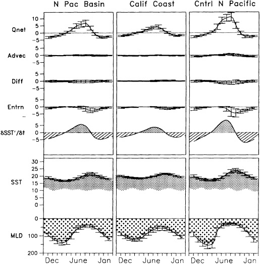
FIGURE 4
Long-term mean and standard deviation of model heat budget terms ![]() , SST (°C), and mixed layer depth (m) for the North Pacific basin, the California Coast, and the central North Pacific regions. Units are 0.1°C mo-1 for heat-budget terms and
, SST (°C), and mixed layer depth (m) for the North Pacific basin, the California Coast, and the central North Pacific regions. Units are 0.1°C mo-1 for heat-budget terms and ![]() .
.
of 1°C and 20 m, respectively. Of the forcing terms in the heat balance, the heat flux has the largest mean and standard deviation (which is in line with previous studies, e.g., Frankignoul, 1985; Haney, 1985; Luksch and von Storch, 1992), followed by the entrainment. The heat flux is in phase with the climatological mean SST tendency, swinging from positive in spring-summer to negative during fall-winter.
Entrainment acts only in one direction: to deepen the mixed layer and to cool the temperature. Entrainment exhibits its maximum effect in fall. Presumably this is because the combination of strong winds and a sharp gradient at the bottom of the mixed layer has its greatest potential in fall. Advection, although a small component, acts in phase with the net heat flux in its mean behavior. Diffusion, which acts to dissipate temperature extremes, is out of phase with the SST and about 90° phase-shifted (but usually of opposite sign) from the heating terms.
The spatial pattern of the primary linkages between heat-budget components and ![]() are shown by the maps of the local correlations over the Pacific basin in Figures 5a through 5c, which appear in the color well. Note that
are shown by the maps of the local correlations over the Pacific basin in Figures 5a through 5c, which appear in the color well. Note that ![]() is approximated here by the centered difference between the SST means for the months before and after the month considered. The correlations, calculated separately for heat flux, entrainment, and advection, were obtained for the set of all months of 1970 through 1988. Correlations between heat flux and
is approximated here by the centered difference between the SST means for the months before and after the month considered. The correlations, calculated separately for heat flux, entrainment, and advection, were obtained for the set of all months of 1970 through 1988. Correlations between heat flux and ![]() (Figure 5a) are relatively high (> 0.6) at nearly all grid points north of 20°N. There is a strong similarity of the model correlations to those derived from observations (Figure 2), with the
(Figure 5a) are relatively high (> 0.6) at nearly all grid points north of 20°N. There is a strong similarity of the model correlations to those derived from observations (Figure 2), with the
strongest correlations (exceeding 0.8) in the lower middle latitudes of the eastern North Pacific and weakest correlations to the northwest, east of Kamchatka. The heat-flux correlations are small in the subtropics, but this is where we prescribed the fluxes to be in phase with the SST via the Newtonian damping scheme. In the tropical Pacific, the correlations are negative and moderately strong, indicating that ocean dynamics processes play a significant role in the model's SST anomaly variability. (Note, however, that the tropical heat flux vs. ![]() relationship may be artificial because the fluxes are prescribed using the Newtonian damping scheme.) Interestingly, in data-available regions of the Southern Hemisphere, the correlations again are relatively strong and positive, implying that heat flux is a substantial component of the model's anomalous temperature budget. For entrainment vs.
relationship may be artificial because the fluxes are prescribed using the Newtonian damping scheme.) Interestingly, in data-available regions of the Southern Hemisphere, the correlations again are relatively strong and positive, implying that heat flux is a substantial component of the model's anomalous temperature budget. For entrainment vs. ![]() (Figure 5c), fairly high (˜ 0.5) correlations occur at scattered locations poleward of about 10°, and right along the equator. Concerning advection (Figure 5b), greatest correlations (> 0.5) with
(Figure 5c), fairly high (˜ 0.5) correlations occur at scattered locations poleward of about 10°, and right along the equator. Concerning advection (Figure 5b), greatest correlations (> 0.5) with ![]() are found in the subtropics and tropics, with strongest centers developed south of the equator between 5°S and 25°S along South America and between 15°S and 15°N north of Australia in the western tropical Pacific. In the North Pacific extratropics, the correlations are generally not very strong, but there is a mild positive correlation region (˜ 0.4) south of the Aleutian Islands, extending into the Gulf of Alaska.
are found in the subtropics and tropics, with strongest centers developed south of the equator between 5°S and 25°S along South America and between 15°S and 15°N north of Australia in the western tropical Pacific. In the North Pacific extratropics, the correlations are generally not very strong, but there is a mild positive correlation region (˜ 0.4) south of the Aleutian Islands, extending into the Gulf of Alaska.
SST Response: Model vs. Observations
As a first look at the skill of the simulation, we examine the time series of area averages of model and observed SST anomalies (Figure 6). Both model and observed anomalies are defined with respect to their monthly mean climatology for the 1970-1988 time interval. We focus on two key regions plus a North Pacific basin average. One key region is the California Coastal region, bounded by 135° and

FIGURE 6
Regional averages of simulated (solid) and observed (dashed) SST anomalies. Correlation coefficients between model and observed are 0.44, 0.71, and 0.67 for the basin-wide, coastal, and central North Pacific regions, respectively.
120°W and by 25° and 45°N, where substantial warming occurred during the 1976-1977 climate shift. The other is in the central North Pacific region, where cooling occurred during the shift, and is bounded by 180° and 150°W and by 30° and 40°N. The basin average was taken in a region corresponding to 130° E to 110°W and 20° to 60°N.
The amplitudes of simulated SST anomalies are slightly lower than the observed anomalies. However, short-term variations in SST, particularly for the coastal region, are remarkably similar considering the uncertainty in the observed heat-flux, TKE, and wind-stress forcing fields. The correlation coefficients between model and observed anomalies are 0.44, 0.71, and 0.67 for the basin-wide, coastal, and mid-Pacific regions, respectively.
Like the observations, the model SST contains variability on monthly to decadal time scales. Reasonable agreement appears in the two key regions, where both major breaks and low-frequency trends are similar. In particular, there is a striking agreement in the longer-time-scale variability, with cooling in the central North Pacific and warming along the Coastal region (Miller et al., 1994a). On the other hand, over the entire North Pacific, the model exhibits a long-term variation in SST, which is not evident in the observations (a residual effect of the long-term variation of heat flux, as described earlier).
The shorter-period model SST variability in Figure 6 has many features in common with the observed SST variability, particularly for the Coastal region. Correlation coefficients between the model and observed SST time series in the central North Pacific and California Coastal regions are 0.67 and 0.71, respectively. In interpreting these, note that the SST contains variability on all time scales, and the correlation is biased toward representing those with the greatest variance. The 1976-1977 warming observed in the Coastal region is clearly evident in the model's response, as is the 1976-1977 cooling of the Mid-Pacific region.
Finally, the spatial pattern of local skill appears in Figure 7 (see color well), which shows the correlation between modeled and observed SST anomalies (all 228 months, 1970-1988). Confirming the validity and impact of the heat flux and wind stress calculated with the bulk formulae, correlations are relatively high (and positive) northward of 20°N, as well as over a broad swath along the tropical Pacific from 165°E to South America. Many grid points exhibit correlations in excess of 0.7. Interestingly, the highest correlations are found in the same area as the largest correlations between the observed latent and sensible fluxes and ![]() in Figure 2. Skill is also poor in areas along the western and northern boundaries and just north of the equator near Central America. Although there is a small region of fairly high skill at 40° to 50°S between 120° and 90°W, the model generally performs poorly in the South Pacific extratropics, where data is scarce. Along the immediate tropical strip (5°N to 5°S), the high skill presumably arises primarily from wind-forced ocean dynamics instead of sea-air fluxes. The model skill is low in the region 10° to 20°N of the North Pacific, where the flux was specified using a Newtonian damping instead of from COADS observations. This suggests that the idealized Newtonian flux scheme is not realistic, and supports the validity of the bulk-formulae fluxes.
in Figure 2. Skill is also poor in areas along the western and northern boundaries and just north of the equator near Central America. Although there is a small region of fairly high skill at 40° to 50°S between 120° and 90°W, the model generally performs poorly in the South Pacific extratropics, where data is scarce. Along the immediate tropical strip (5°N to 5°S), the high skill presumably arises primarily from wind-forced ocean dynamics instead of sea-air fluxes. The model skill is low in the region 10° to 20°N of the North Pacific, where the flux was specified using a Newtonian damping instead of from COADS observations. This suggests that the idealized Newtonian flux scheme is not realistic, and supports the validity of the bulk-formulae fluxes.
For better understanding of the forcing of the anomalous heat budget, ![]() was correlated with monthly anomalies of each of the terms on the right-hand side of Equation 4, with the sum of these four terms, and with the MLD anomaly. Results are shown in Figure 8 for the averages over the North Pacific basin, the California Coastal region, and the central North Pacific region. The relationships in the three regions are quite similar. Consistent with the maps shown in Figure 5, the strongest influence on the mixed-layer temperature anomaly is the net heat-flux anomaly, with correlations usually exceeding 0.7. The next most important term is entrainment, which is important when the mixed layer begins to deepen, and the heat accumulated in summer is vented to the atmosphere. Correlations of
was correlated with monthly anomalies of each of the terms on the right-hand side of Equation 4, with the sum of these four terms, and with the MLD anomaly. Results are shown in Figure 8 for the averages over the North Pacific basin, the California Coastal region, and the central North Pacific region. The relationships in the three regions are quite similar. Consistent with the maps shown in Figure 5, the strongest influence on the mixed-layer temperature anomaly is the net heat-flux anomaly, with correlations usually exceeding 0.7. The next most important term is entrainment, which is important when the mixed layer begins to deepen, and the heat accumulated in summer is vented to the atmosphere. Correlations of ![]() and entrainment are greatest in fall and early winter, some exceeding 0.8. The correlations with entrainment are lowest in spring when mixed-layer depth is decreasing, and remain low until fall when it begins to deepen again. Advection is not as strongly correlated with
and entrainment are greatest in fall and early winter, some exceeding 0.8. The correlations with entrainment are lowest in spring when mixed-layer depth is decreasing, and remain low until fall when it begins to deepen again. Advection is not as strongly correlated with ![]() as the heat flux and the entrainment are, but advection does exhibit correlations exceeding 0.5 in winter for the central North Pacific and
as the heat flux and the entrainment are, but advection does exhibit correlations exceeding 0.5 in winter for the central North Pacific and
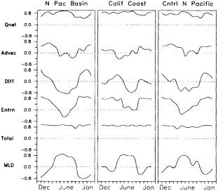
FIGURE 8
Correlation between ![]() and: each of the anomalous model heat-budget forcing terms (right-hand side of Equation 4); their total; and anomalous MLD for the North Pacific basin, California Coastal, and central North Pacific regions. Stratified by month, from 1970-1988.
and: each of the anomalous model heat-budget forcing terms (right-hand side of Equation 4); their total; and anomalous MLD for the North Pacific basin, California Coastal, and central North Pacific regions. Stratified by month, from 1970-1988.
North Pacific basin regions during winter. Model advection is generally not an important influence on SST anomalies in the Coastal region. There is an interesting seasonal cycle in the link between MLD and ![]() , which has its strongest expression for the North Pacific basin average. In fall-early winter (October-January), the two are out of phase: The SST anomaly tends to decrease (
, which has its strongest expression for the North Pacific basin average. In fall-early winter (October-January), the two are out of phase: The SST anomaly tends to decrease (![]() is negative) when the mixed layer is anomalously deep, and vice versa. This implies that when large heat losses and strong wind mixing produce decreasing winter SST anomalies, they also produce a deeper MLD. In summer, the sign of the relationship reverses: The SST anomaly tends to increase when the mixed layer is anomalously deep. This suggests that in summer, when MLD is shallow, the mechanisms that extract heat from the mixed layers produce decreasing SST anomalies when the layer is thinner and the gradient below the mixed layer is stronger (and vice versa).
is negative) when the mixed layer is anomalously deep, and vice versa. This implies that when large heat losses and strong wind mixing produce decreasing winter SST anomalies, they also produce a deeper MLD. In summer, the sign of the relationship reverses: The SST anomaly tends to increase when the mixed layer is anomalously deep. This suggests that in summer, when MLD is shallow, the mechanisms that extract heat from the mixed layers produce decreasing SST anomalies when the layer is thinner and the gradient below the mixed layer is stronger (and vice versa).
Analogous correlations (not shown) were also computed for the Niño 4, Niño 3, and Niño 2 regions along the equator from the international date line to South America. The largest contributions to model SST-anomaly variability in these equatorial regions are entrainment, advection, and diffusion. Strong correlations linking equatorial Pacific SST anomalies to advection and entrainment are indicated by the maps in Figures 5b and 5c. In the tropics, SST anomaly tendencies are generally in phase with MLD anomalies (warming coincides with deeper mixed layers), but not strongly so.
The 1976-1977 SST Shift
To evaluate the model's performance in simulating the spatial pattern of the 1976-1977 shift, the wintertime SST difference field for the six years after the shift (December 1976-February 1977 through December 1981-February 1982) minus the six years before the shift (December 1970-February 1971 through December 1975-February 1976) was calculated, following Graham (1991). Figure 9 (see color well) shows these fields, with the observed SST differences for comparison. The model captures the principal extratropical observations, namely, a warming in the Coastal region and a cooling in the Mid-Pacific region. In the tropics and subtropics, observations contain a swath of warm water throughout the equatorial region and across the southeastern North Pacific. The model captures only a vestige of this warming, which appears mostly in the western half of the tropics. This discrepancy may relate to the use of Newtonian damping rather than observed fluxes in the ± 20° zone. The warming in the equatorial Pacific points to possible dynamic effects due to wind-stress anomalies alone. Mechanisms for the SST shift are suggested by the comparable-difference maps of the winter fields of SLP, net heat flux, and pseudo-rate of kinetic energy transfer by the wind shown in Figures 10a, 10b, and 10c. These maps clearly show a deepened winter Aleutian Low during the post-1976 period (see also Venrick et al., 1987; Trenberth, 1990; Trenberth and Hurrell, 1995, in this volume). The deepened low sustained stronger winds and greater storm activity across the central North Pacific, and generally warmer, moister air masses along the West Coast. This pattern represents a tendency for strong positive PNA patterns in the post-1976 period. These conditions resulted in a large region of increased heat loss in the western and central North Pacific and decreased heat loss in the eastern North Pacific. Increased wind mixing apparently occurred in the central North Pacific, particularly between 30° and 40°N along the southern fringe of the anomalous low-pressure center. Both the heat-flux and wind-mixing patterns are consistent with the SST difference field, shown in Figure 9. Also, the heat-flux difference map is quite similar to the latent-and-sensible heat-flux anomaly maps associated with months having large PNA EOF amplitudes, which appear in Figures 1 and 3.
Inspection of the seasonal time series of the heat-budget components at the individual regions helps to understand
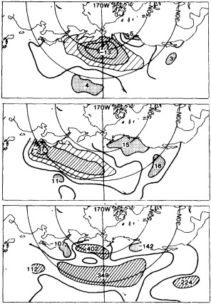
FIGURE 10
Difference fields of observed winter SLP (mb; top), heat flux (W m-2; middle), and {w3}, the pseudo-total kinetic energy (m3 s-3; bottom), for the winters of 1976-77 through 1981-82 minus those of 1970-71 through 1975-76.
the evolution of variability features such as the 1976-1977 shift (Miller et al., 1994a,b). In the Coastal region, heat-flux input tends to be about four times larger than either horizontal advection or entrainment effects. In the mid-Pacific region, in contrast, which is nearer the more variable winds of the storm track, heat-flux input is only twice as large as horizontal advection, and typically the same size as entrainment effects. Diffusion tends to be slightly weaker than horizontal advection, but inspection of the time series shows that diffusion simply acts in opposition to the cumulative effects of the other heating term.
During the six-month period preceding the 1976-1977 climate shift, a long period of warming via heat-flux input occurred in the Coastal region (not shown). Although this period was not particularly strong, it was persistent compared to most of the rest of the time intervals (Miller et al., 1994a). What makes this period particularly striking, however, is that the strongest occurrence (in the 1970-1988 time interval) of warming by horizontal advection took place during fall 1976 and the subsequent winter. Together, these two effects resulted in a mixed layer 10 to 15 m shallower and more than half a degree of warming in the surface temperature. In spite of a strong loss of heat during the late winter of 1977, the system managed to remain in a shallow mixed-layer, warm-SST state through the winter of 1988. Throughout 1977, several months of strong heat-flux cooling began to cool the upper ocean toward the mean, but strong heating in summer 1979 thinned the mixed layer and warmed the SST to such a degree that the mixed-layer warmth persisted into winter 1980.
In the Mid-Pacific region, the 1976-1977 climate shift is likewise instigated by the effects of an anomalously long and strong period of cooling by horizontal advection combined with sizable cooling by heat flux (Figure 11). During the six-year period preceding the shift, anomalously weak entrainment effects (partially due to lower TKE input) serve to maintain the system in a shallow mixed-layer, warm-SST state. In the years following the shift, the effects of stronger entrainment are confined to the summer months.
It therefore appears that the 1976-1977 shift in both the Coastal and Mid-Pacific regions was caused by an unusual atmospheric state that took hold several months before the 1976-1977 winter, and by conditions in the winter atmospheric circulation that persisted for several winters thereafter. This atmospheric circulation produced large-scale shifts in ocean-current advection that acted in concert with large-scale heat-transfer processes to significantly alter the upper-ocean thermal structure, and thus its stratification. The Mid-Pacific region subsequently remained in that perturbed state through the maintenance effects of reduced TKE input.
SUMMARY AND DISCUSSION
Two experimental approaches indicate that bulk parameterizations yield fairly realistic estimates of anomalous sea-

FIGURE 11
Monthly anomaly time series (1970-1988) of simulated surface heat-budget components (net heat-flux term, horizontal advection term, and entrainment term), along with simulated mixed-layer depth (m) and SST (°C), for the central North Pacific. Dashed vertical line marks January 1977, the approximate time at which the large North Pacific SST shift occurred.
air fluxes on seasonal-to-interannual scales over the tropical and northern extratropical oceans. Monthly parameterizations of wind stress and heat flux derived from COADS historical summaries provide reasonable coverage over much of the Pacific basin back to the 1960s. The validity of these derived variables was demonstrated in two ways: (1) by the consistency of the spatial and temporal variability of heat-flux anomalies with independently observed data on the atmospheric circulation and SST tendency; and (2) by the success in simulating two decades of Pacific Ocean SST anomalies with a model driven by the parameterized wind and heat-flux forcings. The bulk parameterizations appear to be adequate for useful diagnoses of several unobserved thermal and dynamic processes (advection, vertical mixing, etc.) that operate in the upper ocean on seasonal-to-decadal time scales.
The model's air-sea heat fluxes were shown to be consistent with two sets of independently observed data. First, the latent and sensible flux anomalies are spatially organized by the atmospheric circulation into systematic patterns about the major cyclonic and anticyclonic features. This organization occurs because the fluxes are determined by wind speed and by air-mass temperature and humidity, which have characteristic structures relating to the general circulation. The flux anomaly/circulation patterns that appear in the North Pacific are confirmed by very similar patterns found
in the North Atlantic (not shown, but see DC1 and DC2). Second, the modeled latent and sensible heat-flux anomaly patterns correspond well to those of SST anomaly tendencies, with regions of increased sea-to-air heat exchange overlying regions of decreasing SST, and vice versa. Monthly SST anomaly tendencies have typical magnitudes of 0.3°C mo−1, and correspond to monthly mean flux anomalies having typical magnitudes of 50 W m−2. Together, the magnitudes of the heat flux and SST tendency are consistent with observed mixed-layer depths.
We also tested the ability of monthly heat fluxes and winds to force a Pacific Ocean general-circulation model over an extended period (1970-1988). The forcings were monthly means of the bulk-formula parameterizations; in this experiment, we superimposed the monthly anomalies of the fluxes and wind parameterizations upon the climatological forcing that was used to spin up the model to its ''stable" annual cycle. In general, the simulation agreed well with observed SST where weather reports (wind, temperature, and humidity) were densely sampled in the extratropical region north of 20°N, but compared quite poorly where they were sparsely sampled. Model SST-anomaly performance was best in the eastern North Pacific between 20°N and 40°N, and along the equatorial strip. It performed poorly between 5°N and 20°N, in the western tropical Pacific, and in most of the southern Pacific. Miller et al. (1994a) showed that the model was remarkably successful in simulating the first three empirical modes of the winter North Pacific SST anomaly.
In the model, anomalous heat fluxes and wind-driven entrainment provide the primary extratropical forcing of the upper-ocean thermal field. The model clearly shows that in the extratropics, the mixed layer deepens with winter anomalous cooling, and shoals with anomalous warming. SST in the region from 5°N to 20°N was poorly simulated, probably because of poor representation of the heat-flux anomalies by a Newtonian scheme in the ± 20° strip. Near the equator, however, where SST anomalies reflect ocean dynamic response to wind forcing, the model anomalies closely resembled those observed.
At lower temporal frequencies, the model captures some important elements of the interannual-to-decadal variability, including aspects of the marked Pacific-basin "shift" that occurred in the winter of 1976-77. Multiple causes appear to be at work in creating the shift, including horizontal advection, anomalous heat fluxes, and wind stirring. This result suggests that a major portion of the shift was forced locally (albeit organized over a large scale) by the atmosphere, rather than by an internal adjustment of the ocean's thermal field. The latter mechanism deserves closer attention, since it is a prime candidate for driving the North Pacific decadal variability exhibited in recent coupled ocean/ atmosphere model results of Latif and Barnett (1994).
These results suggest that ocean models forced by parameterized monthly surface observations are capable of generating important aspects of the anomalous SST variability, on monthly to multi-year time scales. Evidently the lack of synoptic weather variability that characterizes real winds and fluxes is not fatal to the model results. Note, however, that synoptic effects are aggregated into the monthly averages of the fluxes and wind stress, as the nonlinear products within the bulk formulae are taken on an observation-by-observation basis. A more sensitive issue in the simulation of decadal and longer ocean histories is the treatment of the lowest frequencies of the marine data. In the model run conducted here, we removed the largest-spatial-scale, low-frequency (trend-like) behaviors in the wind speed, ΔT, and Δq, since these seemed likely to have arisen from instrumental artifacts. This issue is problematic, though, and longer model runs will be needed to further test these assumptions.
Commentary on the Paper of Cayan et al.
STEPHEN E. ZEBIAK
Lamont-Doherty Earth Observatory
I think Dr. Cayan has given us the opportunity to consider a lot of fairly serious questions, particularly in relation to decadal time scales and ocean modeling. I have noted a few questions that came to my mind. Some of them are really quite general questions, but perhaps they can focus our discussion.
My first two points really deal with the whole issue of using surface heat fluxes for ocean modeling purposes. Dr. Cayan talked about the issue of biases, and I think that when we come to consider decadal time scales, this is an overwhelmingly big problem. The technique that he used was to take components of the flux fields, subject them to EOF analyses, and to look at the first mode and essentially take it out.
I wonder whether we can come to some agreement as to whether that is the best way to proceed. For instance, some of the other talks, such as that of Dr. Wallace yesterday, viewed some of the first empirical orthogonal factors
(EOFs) as the real signal for decadal variability. Dr. Cayan's paper uses the same technique to remove a signal with similar time scales. The products of these terms, as he pointed out, are perhaps a little questionable.
In view of this and of the fact that, as Dr. Cayan noted, the ocean accumulates the errors on long time scales, does it really make sense to try to force ocean models with heat fluxes estimated this way? We do have alternatives. It may be that the traditional place to break the atmosphere and the ocean—the interface—is actually the worst place to make the break. Perhaps it makes more sense, when running an ocean model, to include some sort of planetary boundary-layer model. In that case, the break is made at the top of the boundary layer, which also has problems, but the strength of the coupling at that interface may be less sensitive than that at the ocean surface. Similarly, atmospheric models could be run with ocean mixed layers rather than breaking at the interface, which has often been done.
From Dr. Cayan's results and many others, there is a lot of evidence that the atmosphere forces the ocean on seasonal-to-interannual time scales in middle latitudes, and for the most part it goes the other way around in the tropics. But can we really say that those same relations hold at lower frequency? Our intuition tells us that as we go to a lower and lower frequency, the ocean may be able to contribute more in terms of its dynamics. And in view of the problems with estimating fluxes and so forth, I wonder whether we can answer that question just by looking at surface variables. Perhaps we have to have more information about what goes on beneath the surface of the ocean.
Dr. Cayan's paper points out that the ocean model uses a technique of relaxing the salinity field to the Levitus climatology. It seems to me that the technique introduces a process that is really unphysical, as well as a time scale that is not in the real problem. The alternative is to do other kinds of flux corrections; they also have problems, of course, which I shall deal with later.
Take the issue of climatologies, for example. While Dr. Cayan's paper does not actually show the climatology, I believe it mentions that some of the model results differed considerably from the observations, at least in terms of sea surface temperature.
So how do we deal with mismatches in climatology and things like that that really plague us? One alternative is to improve the model; we would all like to do that, but it is not easy and it takes a long time. The second approach is to ignore them. That has been done, but it is probably not the best choice either. Other methods include relaxation and flux-correction techniques. The flux correction taken to its extreme is essentially making an anomaly model. Of the options, I would propose that until such time as we can improve the models to get the right climatology, thinking in terms of an anomaly model might be the most fruitful approach.
My last point concerns the fact that in his simulations Dr. Cayan got very different-looking EOF structures of simulated SST when he looked at just winter seasons and when he looked at all months, whereas in the observations, the EOF structures looked quite similar. I should like to know what is going on in the model in the other seasons that is different from nature.
Discussion
CAYAN: The time variability I removed is, I think, a wave-like, dynamic phenomenon, not the sort Mike Wallace mentioned. As to whether it makes sense to force ocean models with estimated fluxes, it seems to me that it is accounting for a useful portion of the variability. But I think this model data set can yield some revealing analysis, and Art Miller and I plan to redesign our experiments to incorporate some of what we've been talking about.
LINDZEN: It's always seemed to me that the value of an EOF analysis could be gauged by how many EOFs you need to account for a given amount of variance compared with some objective criterion such as spherical harmonics. If it's, say, one-twentieth as many, EOFs are clearly meaningful.
My other question is on Steve Zebiak's comment on what drives what in which latitudes. Why do you think that the ocean would play a more important role if you extrapolated to longer time scales?
ZEBIAK: I don't think we can completely exclude the possibility that things like gyre circulation could affect SST on those time scales.
BRYAN: I think the ocean's effect is least in the very short and very long time scales, since you reach climatic equilibrium. Its effect should be greatest on the intermediate scales, which of course is what we're concerned with at this workshop.
SARACHIK: Well, it seems to me that in our models the SST determines the mean climate, and so would have the largest effect on long time scales.
LINDZEN: If you take the model to T equals infinity, I think SST would become independent of the ocean.
ROOTH: I want to comment further on Steve's second point, which I think raises the question of what model tests like this are for. The success of an experiment in a simple situation may say that the flux data are reasonably good, but it doesn't say much about the mechanics of the responses for more complicated processes.
SHUKLA: Dan, I'd like to know whether you see the potential for a good mixed-layer model, with some dynamics, that would give us some idea of SST evolution on seasonal time scales.
CAYAN: To do that you'd need to be able to predict the fluxes on fairly high-frequency time scales, not to mention a number of other processes. These models are handicapped, just like the statistical models, by our inability to predict the fluxes.
Atmospheric Observations Reference List
Afanas'eva, V.B., N.P. Esakova, and R.V. Klimentova. 1979. Relation of the planetary upper-air frontal zone to the position of the snow limit during fall and spring. Meteor. Gidrol. 9:110-112.
Agnew, T. 1991. Simultaneous winter sea ice and atmospheric circulation anomaly patterns. Preprints of the Fifth AMS Conference on Climate Variations, Denver, Colo. American Meteorological Society, Boston, Mass., pp. 362-365.
Alexander, M.A. 1990. Simulation of the response of the North Pacific Ocean to the anomalous atmospheric circulation associated with El Niño. Climate Dynamics 5:53-65.
Allan, R.J., and M.R. Haylock. 1993. Circulation features associated with the winter rainfall decrease over southwestern Australia. J. Climate 6:1356-1367.
Allan, R.J., N. Nicholls, P.D. Jones, and I.J. Butterworth. 1991. A further extension of the Tahiti-Darwin SOI, early ENSO events and Darwin pressure. J. Climate 4:743-749.
Alley, R.B., D.A. Meese, C.A. Shuman, A.J. Gow, K.C. Taylor, P.M. Grootes, J.W.C. White, M. Ram, E.D. Waddington, P.A. Mayewski, and G.A. Zielinski. 1993. Abrupt accumulation increase at the Younger Dryas termination in the GISP2 ice core. Nature 362:527-529.
Angell, J.K. 1986. Annual and seasonal global temperature changes in the troposphere and low stratosphere, 1960-85. Mon. Weather Rev. 114:1922-1930.
Arakawa, H. 1957. Climatic change as revealed by the data from the Far East. Weather 12:46-51.
Armstrong, R.L., and M. Hardman. 1991. Monitoring global snow cover. Proceedings of the IEEE International Geoscience and Remote Sensing Symposium (IGARSS '91). IGARSS Volume 4, Institute of Electrical and Electronics Engineers, New York, pp. 1947-1949.
Barnett, T.P. 1984. Long-term trends in surface temperature over the oceans. Mon. Weather Rev. 112:303-312.
Barnett, T.P. 1986. Detection of changes in the global tropospheric temperature field induced by greenhouse gases. J. Geophys. Res. 91:6659-6667.
Barnett, T.P. 1989. A solar-ocean relation: Fact or fiction? Geophys. Res. Lett. 16:803-806.
Barnett, T.P., and P.D. Jones. 1992. Intercomparison of two different Southern Hemisphere sea level pressure data sets. J. Climate 5:92-99.
Barnett, T.P., and M.E. Schlesinger. 1987. Detecting changes in global climate induced by greenhouse gases. J. Geophys. Res. 92:14772-14780.
Barnett, T.P., L. Dümenil, U. Schlese, E. Roeckner, and M. Latif. 1989. The effect of Eurasian snow cover on regional and global climate variations. J. Atmos. Sci. 46:661-685.
Barnett, T.P., M.E. Schlesinger, and X. Jiang. 1991. On greenhouse gas signal detection strategies. In Greenhouse-Gas-Induced Climatic Change: A critical appraisal of simulations and observations. M.E. Schlesinger (ed.). Elsevier, Amsterdam, pp. 537-558.
Barnston, A.G., and R.E. Livezey. 1987. Classification, seasonality, and persistence of low-frequency atmospheric circulation patterns. Mon. Weather Rev. 115:1083-1126.
Barry, R.G. 1983. Arctic Ocean ice and climate: Perspectives on a century of polar research. Ann. Assoc. Am. Geogr. 73:485-501.
Barry, R.G., and R.L. Armstrong. 1987. Snow cover data management: The role of WDC-A for glaciology. Hydrol. Sci. J. 32:281-295.
Berger, A., J.L. Mélice, and I. van der Mersch. 1990. Evolutive spectral analysis of sunspot data over the past 300 years. Phil. Trans. Roy. Soc. London A 330:529-541.
Bevington, P.R. 1969. Data Reduction and Error Analysis for the Physical Sciences. McGraw-Hill, New York, 336 pp.
Bhanu Kumar, O.S.R.U. 1987. Seasonal variation of Eurasian snow cover and its impact on the Indian summer monsoon. In Large Scale Effects of Seasonal Snow Cover. B.E. Goodison, R.G. Barry, and J. Dozier (eds.). IAHS Press, Wallingford, U.K., pp. 51-60.
Bhanu Kumar, O.S.R.U. 1988. Interaction between Eurasian winter snow cover and location of the ridge at the 500 hPa level along 75°E. J. Meteorol. Soc. Japan 66:509-514.
Bjerknes, J. 1959. The recent warming of the North Atlantic. In the Atmosphere and the Sea in Motion, the Rossby Memorial Volume. B. Bolin (ed.). Rockefeller Institute Press in association with Oxford University Press, New York, pp. 65-73.
Bjerknes, J. 1961. Climatic change as an ocean-atmosphere problem. In Proceedings of the Rome Symposium, organized by UNESCO and the World Meteorological Organization, 1961. UNESCO, New York, pp. 297-321.
Bjerknes, J. 1962. Synoptic survey of the interaction of the sea and atmosphere in the North Atlantic. Vilhelm Bjerknes Centenary volume, Geofys. Publikas. XXIV, No. 3, pp. 115-145.
Bjerknes, J. 1964. Atlantic air-sea interaction. Adv. Geophys. 10:1-82.
Black, R.F. 1954. Precipitation at Barrow, Alaska, greater than recorded. AGU Trans. 35(2):203-206.
Blanc, T.V. 1985. Variation of bulk-derived surface flux, stability, and roughness results due to the use of different transfer coefficient schemes. J. Phys. Oceanogr. 15:650-669.
Blanford, H.F. 1884. On the connection of the Himalayan snowfall with dry winds and seasons of drought in India. Proc. Royal Soc. London 37:3-32.
Bleck, R., and D.B. Boudra. 1981. Initial testing of a numerical ocean circulation model using a hybrid coordinate (quasi-isopycnic) vertical coordinate. J. Phys. Oceanogr. 11:755-770.
Bloomfield, P. 1992. Trends in global temperature. Climatic Change 21:1-16.
Bogdanova, E.G. 1966. Investigation of precipitation measurement losses due to the wind. Trans. Main Geophys. Observ. (Leningrad) 195:40-62 (in Russian).
Bogdanova, E.G. 1977. Annual totals and seasonal variation of solid, mixed, and liquid precipitation in mountains of South America. Mat. Glyatsiol. Issled. Khron. Obsuzhd. 30:130-135 (in Russian).
Bolin, B., B.R. Döös, J. Jaeger, and R.A. Warrick (eds.). 1986. The Greenhouse Effect, Climatic Change and Ecosystems: A Synthesis of Present Knowledge. John Wiley and Sons, New York, 541 pp.
Boninsegna, J. A. 1992. South American dendroclimatological records. In Climate Since A.D. 1500. R.S. Bradley and P.D. Jones (eds.). Routledge, London, pp. 446-462.
Bottomley, M., C.K. Folland, J. Hsiung, R.E. Newell, and D.E. Parker. 1990. Global Ocean Surface Temperature Atlas (GOSTA). Joint Project of the Meteorological Office, Bracknell, U.K., and the Massachusetts Institute of Technology. HMSO, London, 20+iv pp. and 313 plates.
Bradley, R.S., and P.D. Jones (eds.). 1992. Climate Since A.D. 1500. Routledge, London, 680 pp.
Bradley, R.S., H.F. Diaz, J.K. Eischeid, P.D. Jones, P.M. Kelly, and C.M. Goodess. 1987. Precipitation fluctuations over northern hemisphere land areas since the mid-19th century. Science 237:171-275.
Briffa, K.R., P.D. Jones, T.S. Bartholin, D. Eckstein, F.H. Schweingruber, W. Karlén, P. Zetterberg, and M. Eronen. 1992a. Fennoscandian summers from A.D. 500: Temperature changes on short and long time scales. Climate Dynamics 7:111-119.
Briffa, K.R., P.D. Jones, and F. Schweingruber. 1992b. Tree-ring density reconstructions of summer temperature patterns across western North America since 1600. J. Climate 5:735-754.
Broecker, W.S., D.M. Peteet, and D. Rind. 1986. Does the ocean-atmosphere system have more than one stable mode of operation? Nature 315:21-26.
Bryan, F. 1986. High-latitude salinity effects and interhemispheric thermohaline circulations. Nature 323:301-304.
Bryan, K., and R. Stouffer. 1991. A note on Bjerknes' hypothesis for North Atlantic variability. J. Mar. Systs. 1:229-241.
Bücher, A., and J. Dessens. 1991. Secular trend of surface temperature at an elevated observatory in the Pyrenees. J. Climate 4:859-868.
Budyko, M.I., and Yu.A. Izrael (eds.). 1987. Anthropogenic climatic changes. Gidrometeoizdat, Leningrad, 406 pp.
Bunting, A.H., M.D. Dennett, J. Elston, and J.R. Milford. 1976. Rainfall trends in the West African Sahel. Quart. J. Roy. Meteorol. Soc. 102:59-64.
Cane, M.A., S.E. Zebiak, and Y. Xue. 1995. Model studies of the long-term behavior of ENSO. In Natural Climate Variability on Decade-to-Century Time Scales. D.G. Martinson, K. Bryan, M. Ghil, M.M. Hall, T.R. Karl, E.S. Sarachik, S. Sorooshian, and L.D. Talley (eds.). National Academy Press, Washington, D.C.
Cao, H.X., J.F.B. Mitchell, and J.R. Lavery. 1992. Simulated diurnal range and variability of surface temperature in a global climate model for present and doubled CO2 climates. J. Climate 5:920-923.
Cardone, V.J., J.G. Greenwood, and M.A. Cane. 1990. On trends in historical marine wind data. J. Climate 3:113-127.
Cayan, D.R. 1990. Variability of Latent and Sensible Heat Fluxes over the Oceans. Ph.D. dissertation, University of California, San Diego, 220 pp.
Cayan, D.R. 1991. Variability of latent and sensible heat fluxes estimated using bulk formulae. Atmos.-Ocean 30:1-42.
Cayan, D.R. 1992a. Latent and sensible heat flux anomalies over the northern oceans: The connection to monthly atmospheric forcing. J. Climate 5:354-369.
Cayan, D.R. 1992b. Latent and sensible heat flux anomalies over the northern oceans: Driving the sea surface temperature. J. Phys. Oceanogr. 22:859-881.
Cayan, D.R., A.J. Miller, T.P. Barnett, N.P. Graham, J.N. Ritchie, and J.M. Oberhuber. 1995. Two decades of a Pacific Ocean GCM simulation driven with monthly surface marine observations. In Natural Climate Variability on Decade-to-Century Time Scales. D.G. Martinson, K. Bryan, M. Ghil, M.M. Hall, T.R. Karl, E.S. Sarachik, S. Sorooshian, and L.D. Talley (eds.). National Academy Press, Washington, D.C.
Cess, R.D., G.L. Potter, J.P. Blanchet, G.J. Boer, R. Colman, and 21 others. 1991. Intercomparison and interpretation of snow-climate feedback processes in seventeen atmospheric general circulation models. Science 253:888-892.
Chang, A.T.C., J.L. Foster, and D.K. Hall. 1987. Nimbus-7 SMMR derived global snow cover parameters. Ann. Glaciol. 9:39-45.
Chang, A.T.C., J.L. Foster, and D.K. Hall. 1990. Satellite sensor estimates of northern hemisphere snow volume. Int. J. Remote Sens. 11:167-171.
Chang, F.-C., and J.M. Wallace. 1987. Meteorological conditions
during heat waves and droughts in the United States Great Plains. Mon. Weather Rev. 115:1253-1269.
Changnon, D., T.B. McKee, and N.J. Doesken. 1993. Annual snow pack patterns across the Rockies: Long-term trends and associated 500-mb synoptic patterns. Mon. Weather Rev. 121:633-647.
Changnon, S.A., Jr. 1987. Climate fluctuations and record-high levels of Lake Michigan. Bull. Amer. Meteorol. Soc. 68:1394-1402.
Chapman, W.L., and J.E. Walsh. 1993. Recent variations of sea ice and air temperature in high latitudes. Bull. Amer. Meteorol. Soc. 74:33-47.
Charlson, R.J., J. Langner, H. Rodhe, C.B. Leovy, and S.G. Warren. 1991. Perturbation of the Northern Hemisphere radiative balance by backscattering from anthropogenic sulfate aerosols. Tellus 43AB:152-163.
Charlson, R.J., S.E. Schwartz, J.M. Hales, R.D. Cess, J.A. Coakley, Jr., J.E. Hansen, and D.J. Hofmann. 1992. Climate forcing by anthropogenic aerosols. Science 255:423-430.
Charney, J.G. 1975. Dynamics of deserts and drought in the Sahel. Quart. J. Roy. Meteorol. Soc. 101:193-202.
Clark, N.E., L. Eber, R.M. Laurs, J.A. Renner, and J.F.T. Saur. 1974. Heat exchange between ocean and atmosphere in the eastern North Pacific for 1961-71. NOAA Technical Report NMFS SSRF-682, Department of Commerce, Seattle, Washington, 108 pp.
Cohen, J., and D. Rind. 1991. The effect of snow cover on the climate. J. Climate 4:689-706.
Cook, E.R., and L.A. Kairiukstis (eds.). 1990. Methods of Dendrochronology: Applications in the Environmental Sciences. Kluwer Academic Publishers, Dordrecht, 394 pp.
Cook, E., T. Bird, M. Peterson, M. Barbetti, B. Buckley, R. D'Arrigo, R. Francey, and P. Tans. 1991. Climatic change in Tasmania inferred from a 1089-year tree-ring chronology of Huon pine. Science 253:1266-1268.
Cook, E.R., T. Bird, M. Peterson, M. Barbetti, B. Buckley, and R. Francey. 1992. The Little Ice Age in Tasmanian tree rings. In Proceedings of the International Symposium on the Little Ice Age. T. Mikami (ed.). Tokyo Metropolitan University, pp. 11-17.
Cook, E.R., B.M. Buckley, and R.D. D'Arrigo. 1995. Interdecadal temperature oscillations in the Southern Hemisphere: Evidence from Tasmanian tree rings since 300 B.C. In Natural Climate Variability on Decade-to-Century Time Scales. D.G. Martinson, K. Bryan, M. Ghil, M.M. Hall, T.R. Karl, E.S. Sarachik, S. Sorooshian, and L.D. Talley (eds.). National Academy Press, Washington, D.C.
Court, A. 1967-68. Climatic Normals as Predictions: Parts I-V. U.S. Air Force Cambridge Research Laboratories scientific reports. NTIS AD-657 358; AD-672 268; AD-687 137, AD-687 138; AD-688 163.
Covey, C., K.E. Taylor, and R.E. Dickinson. 1991. Upper limit for sea-ice-albedo feedback contribution to global warming. J. Geophys. Res. 96:9169-9174.
D'Arrigo, R.D., and G.C. Jacoby, Jr. 1992. Dendroclimatic evidence from northern North America. In Climate Since A.D. 1500. R.S. Bradley and P.D. Jones (eds.). Routledge, London, pp. 296-311.
Davis, R. 1976. Predictability of sea surface temperature and sea level pressure anomalies over the North Pacific Ocean. J. Phys. Oceanogr. 6:249-266.
Deser, C., and M.L. Blackmon. 1993. Surface climate variations over the North Atlantic Ocean during winter: 1900-1989. J. Climate 6:1743-1753.
Deser, C., and M.L. Blackmon. 1995. Surface climate variations over the North Atlantic Ocean during winter: 1900-1989. In Natural Climate Variability on Decade-to-Century Time Scales. D.G. Martinson, K. Bryan, M. Ghil, M.M. Hall, T.R. Karl, E.S. Sarachik, S. Sorooshian, and L.D. Talley (eds.). National Academy Press, Washington, D.C.
Dewey, K.F. 1977. Daily maximum and minimum temperature forecasts and the influence of snow cover. Mon. Weather Rev. 105:1594-1597.
Dewey, K.F., and R. Heim, Jr. 1982. A digital archive of Northern Hemisphere snow cover, November 1966 through December 1980. Bull. Am. Meteorol. Soc. 63:1132-1141.
Dewey, K.F., and R. Heim, Jr. 1983. Satellite observations of variations in Southern Hemisphere snow cover. NOAA Technical Report NESDIS 1, Washington, D.C., 20 pp.
Dey, B., O.S.R.U. Bhanu Kumar, and S.N. Kathuria. 1984. Himalayan snow cover and the Indian summer monsoon activity. Final Report, NSF Grant ATM-8109177, Howard Univ., Washington, D.C., 30 pp.
Diaz, H.F. 1983. Some aspects of major dry and wet periods in the contiguous United States, 1895-1981. J. Clim. Appl. Meteorol. 22:3-16.
Diaz, H.F., and R.S. Bradley. 1995. Documenting natural climatic variations: How different is the climate of the twentieth century from that of previous centuries? In Natural Climate Variability on Decade-to-Century Time Scales. D.G. Martinson, K. Bryan, M. Ghil, M.M. Hall, T.R. Karl, E.S. Sarachik, S. Sorooshian, and L.D. Talley (eds.). National Academy Press, Washington, D.C.
Diaz, H.F., and R.G. Quayle. 1980. The climate of the United States since 1895: Spatial and temporal changes. Mon. Weather Rev. 108:249-266.
Dickson, R.R. 1984. Eurasian snow cover versus Indian monsoon rainfall—An extension of the Hahn-Shukla results. J. Clim. Appl. Meteorol. 23:171-173.
Dickson, R.R., and J. Namias. 1976. North American influence on the circulation and climate of the North Atlantic sector. Mon. Weather Rev. 104:1255-1265.
Dickson, R.R., J. Meincke, S.A. Malmberg, and A.J. Lee. 1988. The "Great Salinity Anomaly" in the northern North Atlantic 1968-1982. Prog. Oceanogr. 20:103-151.
Dirmeyer, P., and J. Shukla. 1993. Observational and modeling studies of the influence of soil moisture anomalies on atmospheric circulation (Review). In Prediction of Interannual Climate Variations. J. Shukla (ed.). Springer-Verlag, New York. pp. 1-24.
Douglas, A.V., D.R. Cayan, and J. Namias. 1982. Large-scale changes in North Pacific and North American weather patterns in recent decades. Mon. Weather Rev. 110:1851-1862.
Dutton, E.G., R.S. Stone, D.W. Nelson, and B.G. Mendonca. 1991. Recent Interannual Variations in Solar Radiation. Cloudiness, and Surface Temperature at the South Pole. J. Climate 4:848-858.
Ebbesmeyer, C.C., D.R. Cayan, D.R. McLain, F.H. Nichols, D.H. Peterson, and K.T. Redmond. 1991. 1976 step in the Pacific climate: Forty environmental changes between 1968-75 and 1977-1984. In Proceedings of the Seventh Annual Pacific Climate (PACLIM) Workshop (Asilomar, April 1990). J.L. Betancourt and V.L. Tharp (eds.). Interagency Ecological Studies Program Technical Report 26, California Department of Water Resources, Sacramento, Calif., pp. 115-126.
Elliott, W.P., and J.K. Angell. 1988. Evidence for changes in Southern Oscillation relationships during the last 100 years. J. Climate 1:729-737.
Elliott, W.P., M.E. Smith, and J.K. Angell. 1991. Monitoring tropospheric water vapor changes using radiosonde data. In Greenhouse-Gas-Induced Climatic Change: A Critical Appraisal of Simulations and Observations. M.E. Schlesinger (ed.). Elsevier, Amsterdam, pp. 311-328.
Enfield, D.B. and L. Cid. 1990. Statistical analysis of El Niño/ Southern Oscillation over the last 500 years. In Toga Notes, Volume 7, Nova University, Dania, Florida, pp. 1-4.
Enting, I.G. 1987. On the use of smoothing splines to filter CO2 data. J. Geophys. Res. 92:10977-10984.
Esbensen, S.K., and Y. Kushnir. 1981. The Heat Budget of the Global Ocean: An atlas based on estimates from surface marine observations. Report No. 29, Climatic Research Institute and Department of Atmospheric Sciences, Oregon State University, Corvallis, Oregon, 219 pp.
Farmer, G. 1988. Seasonal forecasting of the Kenya coast short rains, 1901-1984. J. Climatol. 8:489-497.
Fisher, D.A., and R.M. Koerner. 1983. Ice core study: A climatic link between the past, present and future. In Climatic Change in Canada 3. C.R. Harington (ed.). Syllogeus No. 49, pp. 50-69.
Fleer, H. 1981. Large-Scale Tropical Rainfall Anomalies. Bonner Meteorologische Abhandlungen, No. 26, 114 pp.
Flohn, H. 1986. Singular events and catastrophes now and in climatic history. Naturwissenschaften 73:1851-1862.
Flohn, H., A. Kapala, H.R. Knoche, and H. Machel. 1990. Recent changes of the tropical water and energy budget and of mid-latitude circulations. Climate Dynamics 4:237-252.
Flohn, H., H.R. Kapala, H.R. Knoche, and H. Mächel. 1992. Water vapour as an amplifier of the greenhouse effect: New aspects. Meteorol. Zeitschrift, N.F. 1: 122-138.
Folland, C.K., D.E. Parker, and F.E. Kates. 1984. Worldwide marine temperature fluctuations 1856-1981. Nature 310:670673.
Folland, C.K., T.N. Palmer, and D.E. Parker. 1986. Sahel rainfall and worldwide sea temperatures. Nature 320:602-607.
Folland, C.K., T.R. Karl, and K.Ya. Vinnikov. 1990. Observed climate variations and change. In Climate Change: The IPCC Scientific Assessment. J.T. Houghton, G.J. Jenkins, and J.J. Ephraums (eds.). Prepared for the Intergovernmental Panel on Climate Change by Working Group I. WMO/UNEP, Cambridge University Press, pp. 195-238.
Folland, C.K., J. Owen, M.N. Ward, and A. Colman. 1991. Prediction of seasonal rainfall in the Sahel region using empirical and dynamical methods. J. Forecast. 10:21-56.
Frankignoul, C., 1985. Sea surface temperature anomalies, planetary waves, and air-sea feedback in the middle latitudes. Rev. Geophys. 23:357-390.
Frankignoul, C., and R.W. Reynolds. 1983. Testing a dynamical model for mid-latitude sea surface temperature anomalies. J. Phys. Oceanogr. 13:1131-1145.
Frich, P. 1992. Cloudiness and diurnal temperature range. In Proceedings of the Fifth International Meeting on Statistical Climatology. Environment Canada, Toronto, pp. 91-94.
Friis-Christensen, E., and K. Lassen. 1991. Length of the solar cycle activity closely associated with climate. Science 254:698-700.
Fritts, H.C. 1976. Tree Rings and Climate. Academic Press, London, 567 pp.
Fritts, H.C. 1991. Reconstructing Large-Scale Climatic Patterns from Tree-Ring Data. University of Arizona Press, Tucson, 286 pp.
Fritts, H.C., G.R. Lofgren, and G.A. Gordon. 1979. Variations in climate since 1602 as reconstructed from tree rings. Quat. Res. 12:18-46.
Gall, R., K. Young, R. Schotland, and J. Schmitz. 1992. The recent maximum temperature anomalies in Tucson: Are they real or an instrumental problem? J. Climate 5:657-665.
Ghil, M., and R. Vautard. 1991. Interdecadal oscillations and the warming trend in global temperature time series. Nature 350:324-327.
Gill, A.E., and P.P. Niiler. 1973. The theory of the seasonal variability in the ocean. Deep-Sea Res. 20:141-177.
Giovinetto, M.B., and W. Schwertfeger. 1966. Analysis of a 200-year snow accumulation series from the South Pole . Archiv. Met. Geophys. Biokl. A15:227-250.
Goldenberg, S.B., and J.J. O'Brien. 1981. Time and space variability of tropical Pacific wind stress. J. Phys. Oceanogr. 11:1190-1207.
Golubev, V.V., P.Ya. Groisman, and R.G. Quayle. 1992. An evaluation of the U.S. standard 8-inch nonrecording rain gauge at the Valdai polygon, USSR. J. Atmos. Ocean. Technol. 49:624-629.
Goodison, B.E. 1978. Accuracy of Canadian snow gauge measurements. J. Appl. Meteor. 17:1542-1548.
Goodison, B.E., and P.Y.T. Louie. 1986. Canadian methods for precipitation measurement and correction. In Proceedings of the International Workshop on Correction of Precipitation Measurements. Instruments and Observing Methods Report No. 25, WMO/TD No. 104, World Meteorological Organization, Geneva, pp. 141-145.
Goodison, B.E., and J.R. Metcalfe. 1989. Canadian participation in the WMO Solid Precipitation Measurement Intercomparison: Preliminary results. In Proceedings of the WMO/IAHS/ETH International Workshop on Precipitation Measurement (St. Moritz). Swiss Federal Institute of Technology, Zürich, pp. 121-125.
Goodison, B.E., H.L. Ferguson, and G.A. McKay. 1981. Comparison of point snowfall measurement techniques. In Handbook on Snow: Principles, Processes, Management and Use. D.M. Gray and D.M. Male (eds.). Pergamon Press, Oxford, pp. 200-210.
Goodison, B.E., V.S. Golubev, T. Gunter, and B. Sevruk. 1992. Preliminary results of the WMO Solid Precipitation Measurement Intercomparison. In Proceedings of WMO Technical Conference on Instruments and Methods of Observation (Vienna).
Instruments and Observing Methods Report No. 49, World Meteorological Organization, Geneva, pp. 161-165.
Gordon, A.L., S.E. Zebiak, and K. Bryan. 1992. Climate variability and the Atlantic Ocean. EOS 73:161-165.
Graham, N.E. 1994. Decadal-scale climate variability in the tropical and North Pacific during the 1970s and 1980s: Observations and model results. Climate Dynamics 10:135-162.
Graybill, D.A., and S.G. Shiyatov. 1992. Dendroclimatic evidence from the northern Soviet Union. In Climate Since A.D. 1500. R.S. Bradley and P.D. Jones (eds). Routledge, London, pp. 393-414.
Greatbach, R.J., A.F. Fanning, and A.D. Goulding. 1991. A diagnosis of interpentadal circulation changes in the North Atlantic. J. Geophys. Res. 96:22009-22023.
Gribbin, J. 1979. The search for cycles. In Climatic Change. J. Gribbin (ed.). Cambridge University Press, Cambridge, pp. 139-149.
Groisman, P.Ya. 1991. Unbiased estimates of precipitation change in the Northern Hemisphere extratropics. In Proceedings of the Fifth Conference on Climate Variations (Denver). American Meteorological Society, Boston, pp. 42-45.
Groisman, P.Ya. 1992. Studying the North American precipitation changes during the last 100 years. In Proceedings of the Fifth International Meeting on Statistical Climatology (Toronto). American Meteorological Society, Boston, pp. 75-79.
Groisman, P.Ya., and D.R. Easterling. 1995. Variability and trends of precipitation and snowfall over North America. In Natural Climate Variability on Decade-to-Century Time Scales. D.G. Martinson, K. Bryan, M. Ghil, M.M. Hall, T.R. Karl, E.S. Sarachik, S. Sorooshian, and L.D. Talley (eds.). National Academy Press, Washington, D.C.
Groisman, P.Ya., V.V. Koknaeva, T.A. Belokrylova, and T.R. Karl. 1991. Overcoming biases of precipitation measurement: A history of the USSR experience. Bull. Amer. Meteorol. Soc. 72:1725-1733.
Groisman, P.Ya., R.W. Knight, T.R. Karl, and R.R. Heim, Jr. 1993. Inferences of the North American snowfall and snow cover with recent global temperature changes. In Glaciological Data Report GD-25 (Snow Watch 1992), World Data Center A for Glaciology, Boulder, Colo., pp. 44-51.
Gullett, D.W., and W.R. Skinner. 1992. The State of Canada's Climate: Temperature Change in Canada 1895-1991. SOE Report No. 92-2, Atmospheric Environment Service, Environment Canada, Ottawa, 36 pp.
Haberli, W., P. Maller, P. Allan, and H. Bijsch. 1989. Glacier changes following the Little Ice Age—A survey of the international data base and its perspectives. In Glacier Fluctuations and Climatic Change. J. Oerlemans (ed.). Kluwer Academic Publishers, Dordrecht, 77-101.
Hahn, D.G., and J. Shukla. 1976. An apparent relationship between snow cover and Indian monsoon rainfall. J. Atmos. Sci. 33:2461-2462.
Hall, S.J. 1986. Air Force Global Weather Central Snow Analysis Model. Technical Note 86/001, USAF Airforce Global Weather Central, Offut Air Force Base, Neb., 48 pp.
Halliwell, G.R., and P. Cornillon. 1989. Large scale SST anomalies associated with subtropical fronts in the western North Atlantic during FASINEX. J. Mar. Res. 47:757-775.
Hamilton, K., and R.R. Garcia. 1986. El Niño-Southern Oscillation events and their associated mid-latitude teleconnections 15311841. Bull. Am. Meteorol. Soc. 67:1354-1361.
Hammer, C.U., H.B. Clausen, W. Dansgaard, N. Gundestrup, S.J. Johnsen, and N. Reeh. 1978. Dating of Greenland ice cores by flow models, isotopes, volcanic debris and continental dust. J. Glaciol. 20:3-26.
Haney, R.L. 1985. Mid-latitude sea surface temperature anomalies: A numerical hindcast. J. Phys. Oceanogr. 15:787-799.
Hansen, J.E., and A.A. Lacis. 1990. Sun and dust versus greenhouse gases: An assessment of their relative roles in global climate change. Nature 346:713-718.
Hanson, A.M. 1980. The snow cover of sea ice during the Arctic Ice Dynamics Joint Experiment, 1975-1976. Arct. Alp. Res. 12:215-226.
Hanson, K., G.W. Brier, and G.A. Maul. 1989. Evidence of significant nonrandom behavior in the recurrence of strong El Niño between 1525 and 1988. Geophys. Res. Lett. 16:1181-1184.
Hare, F.K. 1980. Long-term annual surface heat and water balances over Canada and the United States south of 60°N: Reconciliation of precipitation, run-off and temperature fields. Atmos.-Ocean 18(2):127-153.
Harrison, M.S.J. 1983. The southern oscillation, zonal equatorial circulation cells and South African rainfall. In Preprints of the First International Conference on Southern Hemisphere Meteorology. American Meteorological Society, Boston, pp. 302-305.
Hartmann, D.L., M.E. Ockert-Bell, and M.L. Michelsen. 1992. The effect of cloud type on earth's energy balance: Global analysis. J. Climate 5:1157-1171.
Henderson-Sellers, A. 1986. Cloud changes in a warmer Europe. Climatic Change 8:25-52.
Henderson-Sellers, A. 1989. North American total cloud amount variations this century. Glob. Planet. Change 1:175-194.
Henderson-Sellers, A. 1990. Review of our current information about cloudiness changes this century. In Observed Climate Variations and Change: Contributions in Support of Section 7 of the 1990 IPCC Scientific Assessment. D.E. Parker (ed.). Intergovernmental Panel on Climate Change, Geneva, pp. XI.1-XI.12.
Henderson-Sellers, A. 1992. Continental cloudiness changes this century. Geogr. J. 27(3):255-262.
Holloway, P.E. 1991. On the dissipation of internal tides. In Tidal Hydrodynamics. B.B. Parker (ed.). John Wiley and Sons, New York, pp. 449-468.
Hughes, M.G., and D.A. Robinson. 1993. Creating temporally complete snow cover records using a new method for modeling snow depth changes. In Glaciological Data Report GD-25 (Snow Watch 1992), World Data Center A for Glaciology, Boulder, Colo., pp. 150-163.
Hughes, M.K., P.M. Kelly, J.R. Pilcher, and V.C. LaMarche, Jr. (eds.). 1982. Climate from Tree Rings. Cambridge University Press, Cambridge, 223 pp.
Hurst, H.E. 1957. A suggested statistical model of some time series which occur in nature. Nature 180:494.
ICSU/UNEP/UNESCO/WMO. 1993. Draft Plan for Global Climate Observing System . World Meteorological Organization, Geneva, Switzerland.
Ikeda, M. 1990. Decadal oscillations of the air-ice-ocean system in the Northern Hemisphere. Atmos.-Ocean 28:106-139.
Ingram, W.J., C.A. Wilson, and J.F.B. Mitchell. 1989. Modeling climate change: An assessment of sea ice and surface albedo feedbacks. J. Geophys. Res. 94:8609-8622.
IPCC. 1990. Climate Change: The IPCC Scientific Assessment. J.T. Houghton, G.J. Jenkins, and J.J. Ephraums (eds.). Prepared for the Intergovernmental Panel on Climate Change by Working Group I. WMO/UNEP, Cambridge University Press, 365 pp.
IPCC. 1992. Climate Change 1992: The Supplementary Report to the IPCC Scientific Assessment. J.T. Houghton, B.A. Callander, and S.K. Varney (eds.). Prepared for the Intergovernmental Panel on Climate Change by Working Group I. WMO/UNEP, Cambridge University Press, 200 pp.
Isdale, P. 1984. Fluorescent bands in massive corals record centuries of coastal rainfall. Nature 310:578-579.
Isemer, H.-J., and L. Hasse. 1985. The Bunker Climate Atlas of the North Atlantic Ocean . Volume 1: Observations. Springer-Verlag, Berlin, 218 pp.
Isemer, H.-J., and L. Hasse. 1987. The Bunker Climate Atlas of the North Atlantic Ocean. Volume 2: Air-Sea Interactions. Springer-Verlag, Berlin, 252 pp.
Iwasaki, T. 1991. Year-to-year variation of snow cover area in the Northern Hemisphere. J. Meteorol. Soc. Japan 69:209-217.
Jackson, M.C. 1978. Snow cover in Great Britain. Weather 33:298-309.
James, I.N., and P.M. James. 1989. Ultra-low-frequency variability in a simple atmospheric circulation model. Nature 342:53-55.
Johnsen, S.J., W. Dansgaard, H.B. Clausen, and C.C. Langway, Jr. 1972. Oxygen isotope profiles through the Antarctic and Greenland ice sheets. Nature 235:429-434.
Jones, P.A., and A. Henderson-Sellers. 1992. Historical records of cloudiness and sunshine in Australia. J. Climate 5:260-267.
Jones, P.D. 1988. Hemispheric surface air temperature variations: Recent trends and an update to 1987. J. Climate 1:654-660.
Jones, P.D. 1991. Southern Hemisphere sea level pressure data: An analysis and reconstructions back to 1951 and 1911. Int. J. Climatol. 11:585-607.
Jones, P.D. 1992. Maximum and minimum temperature trends over Sudan, 1950-1982. In Proceedings of the International Temperature Workshop. D.E. Parker (ed.). Climate Research Technical Note No. 30, Hadley Centre, UKMO, Bracknell, Berkshire, pp. 19-22.
Jones, P.D., and R.S. Bradley. 1992. Climatic variations in the longest instrumental records. In Climate Since A.D. 1500. R.S. Bradley and P.D. Jones (eds.). Routledge, London, pp. 246-248.
Jones, P.D., and K.R. Briffa. 1995. Decade-to-century-scale variability of regional and hemispheric-scale temperatures. In Natural Climate Variability on Decade-to-Century Time Scales. D.G. Martinson, K. Bryan, M. Ghil, M.M. Hall, T.R. Karl, E.S. Sarachik, S. Sorooshian, and L.D. Talley (eds.). National Academy Press, Washington, D.C.
Jones, P.D., and P.M. Kelly. 1983. The spatial and temporal characteristics of Northern Hemisphere surface air temperature variations. J. Climatol. 3:243-252.
Jones, P.D., and T.M.L. Wigley. 1991. Global and hemispheric anomalies. In Trends '91: A Compendium of Data on Global Change. T.A. Boden, R.J. Sepanski, and F.W. Stoss (eds.). U.S. Department of Energy, Oak Ridge National Laboratory, Environmental Sciences Division Publication No. 3746, pp. 512-517.
Jones, P.D., S.C.B. Raper, R.S. Bradley, H.F. Diaz, P.M. Kelly, and T.M.L. Wigley. 1986a. Northern Hemisphere surface air temperature variations, 1851-1984. J. Clim. Appl. Meteorol. 25:161-179.
Jones, P.D., S.C.B. Raper, R.S. Bradley, H.F. Diaz, P.M. Kelly, and T.M.L. Wigley. 1986b. Southern Hemisphere surface air temperature variations, 1851-1984. J. Clim. Appl. Meteorol. 25:1213-1230.
Jones, P.D., T.M.L. Wigley, and P.B. Wright. 1986c. Global temperature variations between 1861 and 1984. Nature 332:430-434.
Jones, P.D., P.Ya. Groisman, M. Coughlan, N. Plummer, W.-C. Wang, and T.R. Karl. 1990. Assessment of urbanization effects in time series of surface air temperature over land. Nature 347:169-172.
Kagan, R.L. 1979. Averaging of Meteorological Fields. Gidrometeoizdat, Leningrad, 212 pp. (in Russian).
Kaiser, D.P., and V.N. Razuvayev. 1995. Cloud cover and type over the former USSR, 1936-83: Trends derived from the RIHMI-WDC 223-station 6- and 3-hourly meteorological data base. In Proceedings of the Sixth International Meeting on Statistical Climatology. University College, Galway, Ireland, pp. 419-422.
Kalnay, E., and R. Jenne. 1991. Summary of the NMC/NCAR Reanalysis Workshop of April 1991. Bull. Amer. Meteorol. Soc. 72:1897-1904.
Kanamitsu, M., and T.N. Krishnamurti. 1978. Northern summer tropical circulations during drought and normal rainfall months. Mon. Weather Rev. 106:331-347.
Karl, T.R. 1988. Multi-year fluctuations of temperature and precipitation: The gray area of climate change. Climate Change 12:179-197.
Karl, T.R., and P.M. Steurer. 1990. Increased cloudiness in the United States during the first half of the twentieth century: Fact or fiction? Geophys. Res. Lett. 17:1925-1928.
Karl, T.R., and C.N. Williams, Jr. 1986. An approach to adjusting climatological time series for discontinuous inhomogeneities. J. Clim. Appl. Meteorol. 26:1744-1763.
Karl, T.R., G. Kukla, and J. Gavin. 1984a. Decreasing diurnal temperature range in the United States and Canada from 19411980. J. Clim. Appl. Meteorol. 23:1489-1504.
Karl, T.R., R.E. Livezey, and E.S. Epstein. 1984b. Recent unusual mean winter temperatures across the contiguous United States. Bull. Am. Meteorol. Soc. 65:1302-1309.
Karl, T.R., C.N. Williams Jr., and P.J. Young. 1986. A model to estimate the time of observation bias associated with mean monthly maximum, minimum and mean temperatures for the United States. J. Clim. Appl. Meteorol. 25:145-160.
Karl, T.R., H.F. Diaz, and G. Kukla. 1988. Urbanization: Its detection and effect in the United States climate record. J. Climate 1:1099-1123.
Karl, T.R., J.D. Tarpley, R.G. Quayle, H.F. Diaz, D.A. Robinson, and R.S. Bradley. 1989. The recent climate record: What it can and cannot tell us. Rev. Geophys. 27:405-430.
Karl, T.R., C.N. Williams, Jr., F.T. Quinlan, and T.A. Boden. 1990. United States Historical Climatology Network (HCN)
Serial Temperature and Precipitation Data. Report ORNL/ CDIAC-30, NDP-019/R1, Carbon Dioxide Information Analysis Center, Oak Ridge National Laboratory, Oak Ridge, Tenn., 83 pp. plus appendices.
Karl, T.R., G. Kukla, V.N. Razuvayev, M.J. Changery, R.G. Quayle, R.R. Heim, Jr., D.R. Easterling, and C.B. Fu. 1991a. Global warming: Evidence for asymmetric diurnal temperature change. Geophys. Res. Lett. 18:2253-2256.
Karl, T.R., R.R. Heim, Jr., and R.G. Quayle. 1991b. The greenhouse effect in central North America: If not now, when? Science 251:1058-1061.
Karl, T.R., P.Ya. Groisman, R.R. Heim, Jr., and R.W. Knight. 1993a. Recent variations of snow cover and snowfall in North America and their relation to precipitation and temperature variations. J. Climate 6:1327-1344.
Karl, T.R., R.G. Quayle, and P.Ya. Groisman. 1993b. Detecting climate variations and change: New challenges for observing and data management systems. J. Climate 6:1481-1494.
Karl, T.R., P.D. Jones, R.W. Knight, G. Kukla, N. Plummer, V. Razuvayev, K.P. Gallo, J.A. Lindesay, and R.J. Charlson. 1995. Asymmetric trends of daily maximum and minimum temperature: Empirical evidence and possible causes. In Natural Climate Variability on Decade-to-Century Time Scales. D.G. Martinson, K. Bryan, M. Ghil, M.M. Hall, T.R. Karl, E.S. Sarachik, S. Sorooshian, and L.D. Talley (eds.). National Academy Press, Washington, D.C.
Karoly, D.J. 1987. Southern hemisphere temperature trends: A possible greenhouse gas effect? Geophys. Res. Lett. 14:1139-1141.
Karoly, D.J. 1989a. Southern Hemisphere circulation features associated with El Niño-Southern Oscillation events. J. Climate 2:1239-1252.
Karoly, D.J. 1989b. Low frequency variations of the southern hemisphere circulation. In Extended Abstracts, Third International Conference on Southern Hemisphere Meteorology and Oceanography. American Meteorological Society, Boston, pp. 105-109.
Karoly, D.J. 1990. The role of transient eddies in low-frequency zonal variations of the Southern Hemisphere circulation. Tellus 42A:41-50.
Karoly, D.J. 1995. Observed variability of the Southern Hemisphere atmospheric circulation. In Natural Climate Variability on Decade-to-Century Time Scales. D.G. Martinson, K. Bryan, M. Ghil, M.M. Hall, T.R. Karl, E.S. Sarachik, S. Sorooshian, and L.D. Talley (eds.). National Academy Press, Washington, D.C.
Kay, P.A., and H.F. Diaz (eds.). 1985. Problems and Prospects for Predicting Great Salt Lake Levels. Center for Public Affairs and Administration, University of Utah, 309 pp.
Keeling, C.D., and T.P. Whorf. 1995. Decadal oscillations in global temperature and atmospheric carbon dioxide. In Natural Climate Variability on Decade-to-Century Time Scales . D.G. Martinson, K. Bryan, M. Ghil, M.M. Hall, T.R. Karl, E.S. Sarachik, S. Sorooshian, and L.D. Talley (eds.). National Academy Press, Washington, D.C.
Keeling, C.D., R.B. Bacastow, A.F. Carter, S.C. Piper, T.P. Whorf, M. Heimann, W.G. Mook, and H. Roeloffzen. 1989. A three-dimensional model of atmospheric CO2 transport based on observed winds: 1. Analysis of observational data. In Aspects of Climate Variability in the Pacific and the Western Americas. D.H. Peterson (ed.). Geophysical Monograph 55, American Geophysical Union, Washington, D.C., pp. 165-236.
Kelly, P.M., and T.M.L. Wigley. 1992. Solar cycle length, greenhouse forcing, and global climate. Nature 360:328-330.
Kidson, J.W. 1988a. Indices of the Southern Hemisphere zonal wind. J. Climate 1:183-194.
Kidson, J.W. 1988b. Interannual variations in the Southern Hemisphere circulation. J. Climate 1:1177-1198.
Klein, P., and B.L. Hua. 1988. Mesoscale heterogeneity of the wind-driven mixed layer: Influence of a quasigeostrophic flow. J. Mar. Res. 46:495-525.
Klein, S.A., and D.L. Hartmann. 1993. Spurious changes in the ISCCP dataset. Geophys. Res. Lett. 20:455-458.
Klugman, M.R. 1983. Evidence of climate change in United States seasonal precipitation data, 1948-1976. J. Clim. Appl. Meteorol. 22:1367-1376.
Knox, L.J., K. Higuchi, A. Shabbar, and N.E. Sargent. 1988. Secular variation of northern hemisphere 50 kPa geopotential height. J. Climate 1:500-511.
Koerner, R.M. 1977. Devon Island ice cap: Core stratigraphy and paleoclimate. Science 196:15-18.
Kotwicki, V., and P. Isdale. 1991. Hydrology of Lake Frome: El Niño link. Paleogeogr. Paleoclimatol. Paleoecol. 84:87-98.
Kraus, E.B. 1955a. Secular changes of tropical rainfall regimes. Quart. J. Roy. Meteor. Soc. 81:198-210.
Kraus, E.B. 1955b. Secular changes of east coast rainfall regimes. Quart. J. Roy. Meteor. Soc. 81:430-439.
Kruss, P.O., K.A.Y. Khan, F.M.Q. Malik, M. Muslehuddin, and A. Majid. 1992. Cooling over monsoonal Pakistan. In Fifth International Meeting on Statistical Climatology. Environment Canada, Toronto, p. 27.
Kukla, G., and D.A. Robinson. 1979. Accuracy of snow and ice monitoring. In Glaciological Data Report GD-5 (Workshop on Snow Cover and Sea Ice Data), World Data Center A for Glaciology, Boulder, Colo., pp. 91-97.
Kunzi, K.F., S. Patil, and H. Rott. 1982. Snow-cover parameters retrieved from Nimbus-7 scanning multichannel microwave radiometer (SMMR) data. I.E.E.E. Trans. Geosci. Rem. Sen., GE-20, pp. 452-467.
Kuo, C., C. Lindberg, and D. Thomson. 1990. Coherence established between atmospheric carbon dioxide and global temperature. Nature 343:709-714.
Kushnir, Y. 1994. Interdecadal variations in North Atlantic sea surface temperature and associated atmospheric conditions. J. Climate 7:141-157.
Lamb, H.H. 1955. Two-way relationship between snow or ice limit and 1000-500 mb thickness in the overlying atmosphere. Quart. J. Roy. Meteor. Soc. 8:172-189.
Lamb, H.H. 1972. Climate: Present, Past and Future. Volume 1: Fundamentals and Climate Now. Methuen, London, 613 pp.
Lamb, H.H. 1977. Climate: Present, Past and Future. Volume 2: Climatic History and the Future. Methuen, London, 835 pp.
Lamb, P.J. 1978. Large-scale tropical Atlantic surface circulation patterns associated with sub-Saharan weather anomalies: 1967 and 1968. Tellus 30:240-251.
Lamb, P.J. 1982. Persistence of sub-Saharan drought. Nature 299:46-47.
Landsberg, H.E. 1981. The Urban Climate. Academic Press, New York, 285 pp.
Lang, H., and M. Rohrer. 1987. Temporal and spatial variations of the snow cover in the Swiss Alps. In Large Scale Effects of Seasonal Snow Cover. B.E. Goodison, R.G. Barry, and J. Dozier (eds.). IAHS Press, Wallingford, U.K., pp. 79-92.
Lare, A.R., and S.E. Nicholson. 1993. Contrasting conditions of surface water balance in wet years and dry years as a possible land-surface-atmosphere feedback mechanism in the West African Sahel. J. Climate 7:653-668.
Larkin, H.H., Jr. 1947. A comparison of the Alter and Nipher shields for precipitation gages. Bull. Amer. Meteorol. Soc. 28:200-201.
Larson, L.W., and E.L. Peck. 1974. Accuracy of precipitation measurements for hydrologic modeling. Water Resour. Res. 10:857-863.
Latif, M., and T.P. Barnett. 1994. Causes of decadal climate variability over the North Pacific and North America. Science 266:634-637.
Lau, N.C., and M.J. Nath. 1990. A general circulation model study of the atmospheric response to extratropical SST anomalies observed in 1950-79. J. Climate 3:965-989.
Lazier, J.R.N. 1988. Temperature and salinity changes in the deep Labrador Sea 1962-1986. Deep-Sea Res. 35:1247-1253.
Leathers, D.J., and D.A. Robinson. 1993. The association between extremes in North American snow cover extent and United States temperatures. J. Climate 6:1345-1355.
Lehman, S.J., and L.D. Keigwin. 1992. Sudden changes in the North Atlantic circulation during the last deglaciation. Nature 356:757-746.
Leith, C.E. 1973. The standard error of time-average estimates of climatic means. J. Appl. Meteorol. 12:1066-1069.
Levitus, S. 1982. Climatological Atlas of the World Ocean. NOAA Professional Paper 13, U.S. Government Printing Office, Washington, D.C., 173 pp.
Levitus, S. 1989. Interpentadal variability of temperature and salinity at intermediate depths of the North Atlantic Ocean, 197074 versus 1955-59. J. Geophys. Res. 94:6091-6131.
Li, P. 1987. Seasonal snow resources and their fluctuations in China. In Large Scale Effects of Seasonal Snow Cover. B.E. Goodison, R.G. Barry, and J. Dozier (eds.). IAHS Press, Wallingford, U.K., pp. 93-104.
Lindesay, J.A., M.S.J. Harrison, and M.P. Haffner. 1986. The Southern Oscillation and South African rainfall. S. African J. Science 82:196-198.
Lins, H.F. 1985. Streamflow variability in the United States: 1931-1978. J. Clim. Appl. Meteorol. 24:463-471.
Linsley, R.K., Jr., M.H. Kohler, and J.L.H. Paulhus. 1958. Hydrology for Engineers. McGraw-Hill, N.Y., 340 pp.
Liu, W.T., and C. Gautier. 1990. Thermal forcing on the tropical Pacific from satellite data. J. Geophys. Res. 95(C8):13209-13217.
Loder, J.W., and C. Garrett. 1978. The 18.6-year cycle of sea surface temperature in shallow seas due to variations in tidal mixing. J. Geophys. Res. 83:1967-1970.
London, J., S.G. Warren, and C.J. Hahm. 1991. Thirty-year trend of observed greenhouse clouds over the tropical oceans. Adv. Space Res. 11(3):45-49.
Lorenz, E.N. 1986. The index cycle is alive and well. Namias Symposium, Library of Congress No. 86-50752, pp. 188-196.
Lough, J.M. 1986. Tropical Atlantic sea-surface temperatures and rainfall variations in sub-Saharan Africa. Mon. Weather Rev. 114:561-570.
Lough, J.M., and H.C. Fritts. 1990. Historical aspects of El Niño/ Southern Oscillation—Information from tree rings. In Global Ecological Consequences of the 1982-83 El Niño-Southern Oscillation. P.W. Glynn (ed.). Oceanography Series 52, Elsevier, Amsterdam, pp. 285-321.
Luksch, U., and H. von Storch. 1992. Modeling the low-frequency sea surface temperature variability in the North Pacific. J. Climate 5(9):893-906.
Luksch, U., H. von Storch, and E. Maier-Reimer. 1990. Modeling North Pacific SST anomalies as a response to anomalous atmospheric forcing. J. Mar. Syst. 1:51-60.
Lund, I.A. 1963. Map-pattern classification by statistical methods. J. Appl. Meteorol. 2:56-65.
Maley, J. 1976. Les variations du lac Tchad depuis un millénaire: Conséquences paléoclimatiques. Palaeoecol. Africa 9:44-47.
Manabe, S., and R.J. Stouffer. 1988. Two stable equilibria of a coupled ocean-atmosphere model. J. Climate 1:841-866.
Mandelbrot, B.B., and Wallis, J.R. 1969. Some long-run properties of geophysical records. Water Resour. Res. 5:321-340.
Manley, G. 1969. Snowfall in Britain over the past 300 years. Weather 24:428-37.
Manley, G. 1974. Central England temperatures: Monthly means 1659-1972. Quart. J. Roy. Meteorol. Soc. 100:389-405.
Marsden, R.F., L.A. Mysak, and R.A. Myers. 1991. Evidence for stability enhancement of sea ice in the Greenland and Labrador Seas. J. Geophys. Res. (Oceans) 96: 4783-4789.
Markgraf, V., J.R. Dodson, A.P. Kershaw, M.S. McGlone, and N. Nicholls. 1992. Evolution of late Pleistocene and Holocene climates in the circum-South Pacific land areas. Climate Dynamics 6:193-211.
Matson, M., C.F. Ropelewski, and M.S. Varnadore. 1986. An Atlas of Satellite-Derived Northern Hemispheric Snow Cover Frequency. National Oceanic and Atmospheric Administration, Washington, D.C., 75 pp.
Mayewski, P.A., G. Holdsworth, M.J. Spencer, S. Whitlow, M. Twickler, M.C. Morrison, K.K. Ferland, and L.D. Meeker. 1993. Ice core sulfate from three northern hemisphere sites: Source and temperature forcing implications. Atmos. Environ. 27A:2915-2919.
McFarland, G.D. Wilke, and P.W. Harder II. 1987. Nimbus 7 SMMR investigation of snowpack properties in the northern Great Plains for the winter of 1978-1979. I.E.E.E. Trans. Geosci. Rem. Sen. GE-25:35-46.
McGuffie, K., and A. Henderson-Sellers. 1989. Is Canadian cloudiness increasing? Atmos. Ocean 26:608-633.
Meyers, G., J.R. Donguy, and R.K. Reed. 1986. Evaporative cooling of the western equatorial Pacific Ocean by anomalous winds. Nature 323(6088):523-526.
Michaels, P.J., and D.E. Stooksbury. 1992. Global warming: A reduced threat? Bull. Amer. Meteorol. Soc. 73:1563-1577.
Michaelsen, J. 1989. Long-period fluctuations in El Niño amplitude and frequency reconstructed from tree-rings. In Aspects of Climate Variability in the Pacific and the Western Americas. D.H.
Peterson (ed.). Geophysical Monograph 55, American Geophysical Union, Washington, D.C., pp. 69-74.
Michaud, R., and C.A. Lin. 1992. Monthly summaries of merchant ship surface marine observations and implication for climate variability studies. Climate Dynamics 7:45-55.
Miller, A.J. 1992. Large-scale ocean-atmosphere interactions in a simplified coupled model of the mid-latitude wintertime circulation. J. Atmos. Sci. 49:273-286.
Miller, A.J., J.M. Oberhuber, N.E. Graham, T.P. Barnett. 1992. Tropical Pacific Ocean response to observed winds in a layered general circulation model. J. Geophys. Res. 97:7317-7340.
Miller, A.J., D.R. Cayan, T.P. Barnett, N.E. Graham, and J.M. Oberhuber. 1994a. Interdecadal variability of the Pacific Ocean: Model response to observed heat flux and wind stress anomalies. Climate Dynamics 9:287-302.
Miller, A.J., D.R. Cayan, T.P. Barnett, N.E. Graham, and J.M. Oberhuber. 1994b. The 1976-77 climate shift of the Pacific Ocean. Oceanography 7:21-26.
Milly, P.C.D. 1992. Potential evaporation and soil moisture in general circulation models. J. Climate 5:209-226.
Mintz, Y. 1984. The sensitivity of numerically simulated climates to land surface boundary conditions. In The Global Climate. J. Houghton (ed.). Cambridge University Press, pp. 79-105.
Mitchell, J.M., Jr. 1976. An overview of climate variability and its causal mechanisms. Quat. Res. 6:481-493.
Mo, K.C., and H. van Loon. 1984. Some aspects of the interannual variation of mean monthly sea level pressure on the Southern Hemisphere. J. Geophys. Res. 89D:9541-9546.
Mo, K.C., and G.H. White. 1985. Teleconnections in the Southern Hemisphere. Mon. Weather Rev. 113:22-37.
Mysak, L.A. 1991. Current and Future Trends in Arctic Climate Research: Can Changes in the Arctic Sea Ice be Used as an Early Indicator of Global Warming? Centre for Climate and Global Change Research Report No. 91-1, McGill University, Montreal.
Mysak, L.A., and D.K. Manak. 1989. Arctic sea-ice extent and anomalies, 1953-1984. Atmos.-Ocean 27:376-405.
Mysak, L.A., D.K. Manak, and R.F. Marsden. 1990. Sea-ice anomalies observed in the Greenland and Labrador Seas during 1901-1984 and their relation to an interdecadal Arctic climate cycle. Climate Dynamics 5:111-133.
Nagler, T., and H. Rott. 1991. Intercomparison of snow mapping algorithms over Europe using SSM/I data. Report to the SSM/ I Products Working Team, World Data Center A for Glaciology, Boulder, Colo., 12 pp.
Namias, J. 1962. Influence of abnormal heat sources and sinks on atmospheric behavior. Proceedings, Symposium on Numerical Weather Prediction. Meteorological Society of Japan, Tokyo, pp. 615-627.
Namias, J. 1966. Nature and possible causes of the northeastern United States drought during 1962-65. Mon. Weather Rev. 94:543-554.
Namias, J. 1972. Large-scale and long-term fluctuations in some atmospheric and oceanic variables. Nobel Symposium 20:27-48.
Namias, J. 1981. Snow covers in climate and long-range forecasting. Glaciological Data GD-11 (Snow Watch 1980), World Data Center A for Glaciology, Boulder, Colo., pp. 13-26.
Namias, J. 1985. Some empirical evidence for the influence of snow cover on temperature and precipitation. Mon. Weather Rev. 113:1542-1553.
National Climatic Data Center (NCDC). 1991. Climate Variations Bulletin, Historical Climatology Series 4-7, NOAA NCDC, Asheville, N.C., 35 pp.
National Geophysical Data Center (NGDC). 1988. Data Announcement 88-MGG-02, NOAA, Boulder, Colo. 1 p.
National Geophysical Data Center (NGDC). 1989. Solar Indices Bulletin. NOAA NGDC, Solar-Terrestrial Physics Division, Boulder, Colo.
National Research Council (NRC). 1982. Carbon Dioxide and Climate: A Second Assessment. National Academy Press, Washington, D.C., 72 pp.
Newell, N.E., R.E. Newell, J. Hsiung, and W. Zhongxiang. 1989. Global marine temperature variation and the solar magnetic cycle. Geophys. Res. Lett. 16:311-314.
Newell, R.E., and J.W. Kidson. 1984. African mean wind changes in Sahelian wet and dry periods. J. Climatol. 4:1-7.
Nicholson, S.E. 1978. Climatic variations in the Sahel and other African regions during the past five centuries. J. Arid Environ. 1:3-24.
Nicholson, S.E. 1979a. The methodology of historical climate reconstruction and its application to Africa. J. African Hist. 20:3-24.
Nicholson, S.E. 1979b. Revised rainfall series for the West African subtropics. Mon. Weather Rev. 107:620-623.
Nicholson, S.E. 1981. The historical climatology of Africa. In Climate and History. T.M.L. Wigley, J.J. Ingram, and G. Farmer (eds.). Cambridge University Press, pp. 249-270.
Nicholson, S.E. 1983. Sub-Saharan rainfall in the years 19761980: Evidence of continued drought. Mon. Weather Rev. 111:1646-1654.
Nicholson, S.E. 1986. The spatial coherence of African rainfall anomalies: Interhemispheric teleconnections. J. Clim. Appl. Meteorol. 25:1365-1381.
Nicholson, S.E. 1989. African drought: Characteristics, causal theories, and global teleconnections. In Understanding Climate Change. A. Berger, R.E. Dickinson, and J.W. Kidson (eds.). American Geophysical Union, Washington, D.C., pp. 79-100.
Nicholson, S.E. 1993. An overview of African rainfall fluctuations of the last decade. J. Climate 6:1463-1466.
Nicholson, S.E. 1994. Recent rainfall fluctuations in Africa and their relationships to past conditions over the continent. Holcene 4:121-131.
Nicholson, S.E. 1995. Variability of African rainfall on interannual and decadal time scales. In Natural Climate Variability on Decade-to-Century Time Scales. D.G. Martinson, K. Bryan, M. Ghil, M.M. Hall, T.R. Karl, E.S. Sarachik, S. Sorooshian, and L.D. Talley (eds.). National Academy Press, Washington, D.C.
Nicholson, S.E., and D. Entekhabi. 1986. The quasi-periodic behavior of rainfall variability in Africa and its relationship to the Southern Oscillation. Arch. Meteor. Geophys. Bioklimatol. A34:311-348.
Nicholson, S.E., and D. Entekhabi. 1987. Rainfall variability in equatorial and Southern Africa: Relationships with sea-surface temperatures along the southwestern coast of Africa. J. Clim. Appl. Meteorol. 26:561-578.
Nicholson, S.E., J. Kim, and J. Hoopingarner. 1988. Atlas of
African Rainfall and Its Interannual Variability. Florida State University, Tallahassee, 252 pp.
Nitta, T., and S. Yamada. 1989. Recent warming of tropical sea surface temperature and its relationship to the Northern Hemisphere circulation. J. Meteorol. Soc. Japan 67:375-383.
North, G.R., T.L. Bell, R.F. Calahan, and F.J. Moeng. 1982. Sampling errors in the estimation of empirical orthogonal functions. Mon. Weather Rev. 110:699-706.
Nyenzi, B.S. 1988. Mechanisms of East African Rainfall Variability. M.S. Thesis, Department of Meteorology, Florida State University, Tallahassee, 184 pp.
Oberhuber, J.M. 1988. An Atlas Based on the COADS Data Set: The budgets of heat, buoyancy, and turbulent kinetic energy at the surface of the global ocean. Report No. 15, Max-Planck-Institut für Meteorologie, Hamburg.
Oberhuber, J.M. 1993. Simulation of the Atlantic circulation with a coupled sea ice-mixed layer-isopycnal general circulation model. Part I: Model description; Part II: Model experiment. J. Phys. Oceanogr. 22:808-845.
Ogallo, L. 1979. Rainfall variability in Africa. Mon. Weather Rev. 107:1133-1139.
Ogallo, L. 1987. Relationships between seasonal rainfall in East Africa and the Southern Oscillation . J. Climatol. 7:1-13.
Palmer, T.N., and D.A. Mansfield. 1986. A study of wintertime circulation anomalies during past El Niño events using a high resolution general circulation model. II: Variability of the seasonal mean response. Quart. J. Roy. Meteorol. Soc. 1 12:639-660.
Palmer, T.N., and Z. Sun. 1985. A modeling and observational study of the relationship between sea surface temperature in the north-west Atlantic and the atmospheric general circulation. Quart. J. Roy. Meteor. Soc. 111:947-975.
Paltridge, G., and S. Woodruff. 1981. Changes in global surface temperature from 1880 to 1977 derived from historical records of sea surface temperature. Mon. Weather Rev. 109:2427-2434.
Parungo, F., J.F. Boatman, H. Sievering, S. Wilkinson, and B.B. Hicks. 1994. Trends in global marine cloudiness and anthropogenic sulfur. J. Climate 7:434-440.
Pavia, E.G., and J.J. O'Brien. 1986. Waybill statistics of wind speed over the ocean. J. Climate Appl. Meteorol. 25:1324-1332.
Peck, E.L. 1991. Hydrometeorological Data Collection Design and Analysis for the Lake Ontario Drain Basin: Final Report, Phase 1. Coordinating Committee on Great Lakes Basin Hydraulic and Hydrometeorologic Data, Hydrometeorology and Modeling Subcommittee, International Joint Commission , Washington, D.C.
Penner, J.E., R.E. Dickinson, and C.A. O'Neill. 1992. Effects of aerosol from biomass burning on the global radiation budget. Science 256:1432-1433.
Petersen, R.A., and J.E. Hoke. 1989. The effect of snow cover on the Regional Analysis and Forecast System (RAFS) low-level forecasts. Wea. Forecast. 4:253-257.
Pfister, C. 1985. Snow cover, snow lines and glaciers in Central Europe since the 16th century. In The Climatic Scene. George Allen and Unwin, Winchester, Mass., pp. 154-174.
Pittock, A.B. 1984. On the reality, stability and usefulness of Southern Hemisphere teleconnections. Aust. Meteorol. Mag. 32:75-82.
Plantico, M.S., T.R. Karl, G. Kukla, and J. Gavin. 1990. Is recent climate change across the United States related to rising levels of anthropogenic greenhouse gases? J. Geophys. Res. 95:16617-16637.
Plummer, N., Z. Lin, and S. Torok. 1995. Trends in the diurnal temperature range over Australia since 1951. Atmos. Res. 237:79-86.
Posmentier, E.S., M.A. Cane, and S.E. Zebiak. 1989. Tropical Pacific trends since 1960. J. Climate 2:731-736.
Press, W.H., B.P. Flannery, S.A. Teukolsky, and W.T. Vetterling. 1989. Numerical Recipes (FORTRAN Version). Cambridge University Press, New York, 702 pp.
Quayle, R.G., D.R. Easterling, T.R. Karl, and P.M. Hughes. 1991. Effects of recent thermometer changes in the cooperative station network. Bull. Amer. Meteorol. Soc. 72:1718-1723.
Quinn, W.H., and V.T. Neal. 1992. The historic record of El Niño events. In Climate Since A.D. 1500. R.A. Bradley and P.D. Jones (eds.). Routledge Press, London, pp. 623-648.
Quinn, W.H., V.T. Neal, and S.E.A. de Mayolo. 1987. El Niño occurrences over the past four and a half centuries. J. Geophys. Res. 92:14449-14461.
Ramage, C.S. 1987. Secular change in reported surface wind speed over the ocean . J. Climate Appl. Meteorol. 26:525-529.
Rasmusson, E., X. Wang, and C.F. Ropelewski. 1995. Secular variability of the ENSO cycle. In Natural Climate Variability on Decade-to-Century Time Scales. D.G. Martinson, K. Bryan, M. Ghil, M.M. Hall, T.R. Karl, E.S. Sarachik, S. Sorooshian, and L.D. Talley (eds.). National Academy Press, Washington, D.C.
Reinsch, C.H. 1967. Smoothing by spline functions. Num. Math. 10:177-183.
Riehl, H., M. el-Bakary, and J. Meitin. 1979. Nile river discharge. Mon. Weather Rev. 107:1546-1553.
Rind, D., D. Peteet, W. Broecker, A. McIntyre, and W. Ruddiman. 1986. The impact of cold North Atlantic sea surface temperatures on climate: Implications for the younger Dryas cooling (1110K). Climate Dynamics 1:3-33.
Rind, D., R. Goldberg, and R. Ruedy. 1989. Change in climate variability in the 21st century. Climate Change 14:5-37.
Robinson, D.A. 1989. Evaluation of the collection, archiving and publication of daily snow data in the United States. Phys. Geog. 10:120-130.
Robinson, D.A. 1993a. Historical daily climatic data for the United States. In Preprints of the Eighth Conference on Applied Climate (Anaheim). American Meteorological Society, Boston, Mass., pp. 264-269.
Robinson, D.A. 1993b. Monitoring Northern Hemisphere snow cover. In Glaciological Data Report GD-25 (Snow Watch 1992), World Data Center A for Meteorology, Boulder, Colo., pp. 1-25.
Robinson, D.A. 1995. Decadal variations of snow cover. In Natural Climate Variability on Decade-to-Century Time Scales. D.G. Martinson, K. Bryan, M. Ghil, M.M. Hall, T.R. Karl, E.S. Sarachik, S. Sorooshian, and L.D. Talley (eds.). National Academy Press, Washington, D.C.
Robinson, D.A., and K.F. Dewey. 1990. Recent secular variations in the extent of Northern Hemispheric snow cover. Geophys. Res. Lett. 17:1557-1560.
Robinson, D.A., F.T. Keimig, and K.F. Dewey. 1991. Recent variations in Northern Hemisphere snow cover. In Proceedings
of the 15th Annual Climate Diagnostics Workshop. NOAA National Weather Service, Washington, D.C., pp. 219-224.
Robinson, D.A., M.C. Serreze, R.G. Barry, G. Scharfen, and G. Kukla. 1992. Interannual variability of snow melt and surface albedo in the Arctic basin. J. Climate 5:1109-1119.
Robinson, W.A. 1992. The dynamics of the zonal index in a simple model of the atmosphere. Tellus 43A:295-305.
Robock, A., and J.W. Tauss. 1986. Effects of snow cover and tropical forcing on mid-latitude monthly mean circulation. Glaciological Data GD-18 (Snow Watch 1985), World Data Center A for Glaciology, Boulder, Colo., pp. 207-214.
Rodhe, H., and H. Virji. 1976. Trends and periodicities in East African rainfall data. Mon. Weather Rev. 104:307-315.
Roeckner, E., K. Arpe, L. Bengtsson, S. Brinkop, L. Domenil, M. Esch, E. Kirk, F. Lunkeit, M. Ponater, B. Rockel, R. Sausen, U. Schlese, S. Schubert, and M. Windelband. 1992. Simulation of the Present-Day Climate with the ECHAM Model: Impact of model physics and resolution. Report No. 93, Max-Planck-Institut für Meteorologie, Hamburg.
Rogers, J.C., and H. van Loon. 1982. Spatial variability of sea level pressure and 500 mb height anomalies over the Southern Hemisphere. Mon. Weather Rev. 110:1375-1392.
Ropelewski, C.F., and M.S. Halpert. 1987. Global and regional scale precipitation and temperature patterns associated with El Niño/Southern Oscillation. Mon. Weather Rev. 115:1606-1626.
Ropelewski, C.F, A. Robock, and M. Matson. 1984. Comments on ''An apparent relationship between Eurasian spring snow cover and the advance period of the Indian summer monsoon." J. Clim. Appl. Meteorol. 23:341-342.
Rossow, W.B., and B. Cairns. 1995. Monitoring changes of clouds. Climatic Change 31:305-347.
Rowell, D.P., C.K. Folland, K. Maskell, J.A. Owen, and M.N. Ward. 1992. Modeling the influence of global sea surface temperature on the variability and predictability of seasonal Sahel rainfall. Geophys. Res. Lett. 19:905-908.
Rowell, D.P., C.K. Folland, K. Maskell, and M.N. Ward. 1995. Variability of summer rainfall over tropical north Africa (19061992): Observations and modeling. Quart. J. Roy. Meteor. Soc. 121:669-704.
Saltzman, B. (ed.). 1983. Theory of Climate. Volume 25, Advances in Geophysics, Academic Press, New York, 505 pp.
Sanderson, M. 1975. A comparison of Canadian and United States standard methods of measuring precipitation. J. Appl. Meteorol. 14:1197-1199.
Schlesinger. M.E. 1984. Climate model simulations of CO2 induced climatic change. Adv. Geophys. 26:141-235.
Schlesinger, M.E. (ed.). 1991. Greenhouse-Gas-Induced Climatic Change: A Critical Appraisal of Simulations and Observations. Elsevier, Amsterdam, 615 pp.
Schlesinger, M.E., and J.F.B. Mitchell. 1985. Model projection of the equilibrium climatic response to increased carbon dioxide. In Projecting the Effects of Increasing Carbon Dioxide. M.C. MacCracken and F.M. Luther (eds.). Report DOE/ER-0237, U.S. Department of Energy, pp. 57-80.
Sellers, W.D. 1965. Physical Climatology. University of Chicago Press, 272 pp.
Semazzi, F.H.M., V. Mehta, and Y.C. Sud. 1988. An investigation of the relationship between sub-Saharan rainfall and global sea surface temperatures. Atmos.-Ocean 26:118-138.
Sevruk, B. 1982. Methods of correction for systematic error in point precipitation measurement for operational use. Operational Hydrology Report No. 21, World Meteorological Organization, Geneva, 91 pp.
Sevruk, B., and W.R. Hamon. 1984. International Comparison of National Precipitation Gauges with a Reference Pit Gauge. Instruments and Observing Methods Report No. 17, World Meteorological Organization, Geneva, 111 pp.
Shea, D., R. Jenne, and C. Ropelewski. 1992. NCAR data sets with daily maximum and minimum temperatures. In Proceedings of the International Temperature Workshop. D.E. Parker (ed.). Climate Research Technical Note No. 30, Hadley Centre, UKMO, Bracknell, Berkshire, pp. 27-29.
Shiotani, M. 1990. Low-frequency variations of the zonal mean state of the Southern Hemisphere troposphere . J. Meteorol. Soc. Japan 68:461-471.
Shukla, J. 1995. The initiation and persistence of the Sahel drought. In Natural Climate Variability on Decade-to-Century Time Scales. D.G. Martinson, K. Bryan, M. Ghil, M.M. Hall, T.R. Karl, E.S. Sarachik, S. Sorooshian, and L.D. Talley (eds.). National Academy Press, Washington, D.C.
Skaggs, R.H. 1975. Drought in the United States, 1931-40. Ann. Assoc. Amer. Geogr. 65:391-402.
Slutz, R.J., S.J. Lubker, J.D. Hiscox, S.D. Woodruff, R.L. Jenne, D.H. Joseph, P.M. Steurer, and J.D. Elms. 1985. Comprehensive Ocean-Atmosphere Data Set: Release I. Climate Research Program, NOAA Environmental Research Laboratories, Boulder, Colo., 268 pp. (NTIS PB86-105723).
Solow, A.R. 1987. Testing for climate change: An application of the two-phase regression mode. J. Clim. Appl. Meteorol. 26:1401-1405.
Sonett, C.P. 1983. Is the sunspot spectrum really so complicated? In Weather and Climate Responses to Solar Variations. B.M. McCormac (ed.). Colorado Associated University Press, Boulder, pp. 607-613.
Spencer, R.N., and J.R. Christy. 1990. Precise monitoring of global temperature trends from satellites. Science 247:1558-1562.
Stocker, T.F., and L.A. Mysak. 1992. Climatic fluctuations on the century time scale: A review of high-resolution proxy data and possible mechanisms. Climatic Change 20:227-250.
Szeredi, I., and D.J. Karoly. 1987a. The vertical structure of monthly fluctuations of the Southern Hemisphere troposphere. Aust. Meteorol. Mag. 35:19-30.
Szeredi, I., and D.J. Karoly. 1987b. The horizontal structure of monthly fluctuations of the Southern Hemisphere troposphere from station data. Aust. Meteorol. Mag. 35:119-129.
Taljaard, J.J., W. Schmitt, and H. van Loon. 1961. Frontal analysis with application to the Southern Hemisphere. Notos 10:25-58.
Taylor, P.K. 1984. The determination of surface fluxes of heat and water by satellite microwave radiometry and in situ measurements. In Large-Scale Oceanographic Experiments and Satellites. C. Gautier and M. Fixe (eds.). Series C: Mathematical and Physical Sciences, Vol. 128, pp. 223-246.
Thiessen, A.H. 1911. Precipitation averages for large areas. Mon. Weather Rev. 39:1082-1084.
Thompson, L.G., E. Mosley-Thompson, and B.M. Arnao. 1984.
El Niño-Southern Oscillation events recorded in the stratigraphy of the tropical Quelccaya ice cap, Peru. Science 226:50-53.
Thompson, L.G., E. Mosley-Thompson, W. Dansgaard, and P.M. Grootes. 1986. The Little Ice Age as recorded in the stratigraphy of the tropical Quelccaya ice cap. Science 234:361-364.
Thompson, L.G., E. Mosley-Thompson, M.E. Davis, J. Bolzan, J. Dai, N. Gundestrup, T. Yao, X. Wu, L. Klein, and Z. Zichu. 1990. Glacial stage ice core records from the subtropical Dunde ice cap, China. Ann. Glaciol. 14:288-297.
Thompson, L.G., E. Mosley-Thompson, M.E. Davis, P.-N, Lin, K.A. Henderson, J. Cole-Dai, J.F. Bolzan, and K.-B. Liu. 1995. Late glacial stage and Holocene tropical ice core records from Huascaran, Peru. Science 269:46-50.
Toomig, K.G. 1981. Correlation of mean annual albedo and short-wave radiation balance with these parameters in early spring. Meteor. Gidrol. 5:48-52.
Toussoun, O. 1923. Mémoire sur l'histoire du Nil. Mém. Inst. Égypte 9:63-213.
Treidl, R.A. 1970. A case study of warm air advection over a melting snow surface. Bound. Layer Meteorol. 1:155-168.
Trenberth, K.E. 1976. Fluctuations and trends in indices of the Southern Hemisphere circulation. Quart. J. Roy. Meteorol. Soc. 102:65-75.
Trenberth, K.E. 1979. Interannual variability of the 500 mb zonal mean flow in the Southern Hemisphere. Mon. Weather Rev. 107:1515-1524.
Trenberth, K.E. 1984. Interannual variability of the Southern Hemisphere circulation: Representativeness of the year of the Global Weather Experiment. Mon. Weather Rev. 112:108-123.
Trenberth, K.E. 1990. Recent observed interdecadal climate changes in the Northern Hemisphere. Bull. Amer. Meteorol. Soc. 71:988-993.
Trenberth, K.E. (ed.). 1992. Climate Systems Modeling. Cambridge University Press, 788 pp.
Trenberth, K.E., and G.W. Branstator. 1992. Issues in establishing causes of the 1988 drought over North America. J. Climate 5:159-172.
Trenberth, K.E., and J.R. Christy. 1985. Global fluctuations in the distribution of atmospheric mass. J. Geophys. Res. 90:8042-8052.
Trenberth, K.E., and J.W. Hurrell. 1995. Decadal climate variations in the Pacific. In Natural Climate Variability on Decade-to-Century Time Scales. D.G. Martinson, K. Bryan, M. Ghil, M.M. Hall, T.R. Karl, E.S. Sarachik, S. Sorooshian, and L.D. Talley (eds.). National Academy Press, Washington, D.C.
Troup, A.J. 1965. The Southern Oscillation. Quart. J. Roy. Meteorol. Soc. 91:490-506.
Tyson, P.D. 1980. Temporal and spatial variation of rainfall anomalies in Africa south of latitude 22° during the period of meteorological record. Climate Change 2:363-371.
U.S. Department of Commerce. 1950. Census of Agriculture. Irrigation of Agricultural Levels. Vol. III. (Available through the U.S. Government Printing Office.)
U.S. Department of Commerce. 1988. Farm and Ranch Irrigation Survey. Vol. 3, Part 1. (Available through the U.S. Government Printing Office.)
van Loon, H., and J. Williams. 1978. The association between mean temperature and interannual variability. Mon. Weather Rev. 106:1012-1017.
Venrick, E.L., J.A. McGowan, D.R. Cayan, and T. Hayward. 1987. Climate and chlorophyll a: Long-term trends in the central North Pacific Ocean. Science 238:70-72.
Villalba, R. 1990. Climatic fluctuations in northern Patagonia during the last 1000 years as inferred from tree-ring records. Quat. Res. 34: 346-360.
Villalba, R., J.A. Boninsegna, and D.R. Cobos. 1989. A tree-ring reconstruction of summer temperature between A.D. 1500 and 1974 in western Argentina. In Extended Abstracts, Third International Conference on Southern Hemisphere Meteorology and Oceanography. American Meteorological Society, Boston, pp. 196-197.
Vining, K.C., and J.F. Griffiths. 1985. Climatic variability at ten stations across the United States. J. Clim. Appl. Meteorol. 24:363-370.
Vinnikov, K.Ya., P.Ya. Groisman, and K.M. Lugina. 1900. Empirical data on contemporary global climate changes (temperature and precipitation). J. Climate 3:662-677.
Wahl, E.W. 1968. A comparison of the climate of the eastern United States during the 1830's with the current normals. Mon. Weather Rev. 96:73-82.
Walker, G.R. 1910. Correlations in seasonal variations of weather. Mem. India Meteorol. Dept. 21:22-45.
Walker, J., and P.R. Rowntree. 1977. The effect of soil moisture on circulation and rainfall in a tropical model. Quart. J. Roy. Meteorol. Soc. 103:29-46.
Wallace, J.M., and D.S. Gutzler. 1981. Teleconnections in the geopotential height field during the Northern Hemisphere winter. Mon. Weather Rev. 109:784-812.
Wallace, J.M., C. Smith, and Q. Jiang. 1990. Spatial patterns of atmosphere/ocean interaction in the northern winter. J. Climate 3:990-998.
Walsh, J.E. 1995. Continental snow cover and climate variability. In Natural Climate Variability on Decade-to-Century Time Scales. D.G. Martinson, K. Bryan, M. Ghil, M.M. Hall, T.R. Karl, E.S. Sarachik, S. Sorooshian, and L.D. Talley (eds.). National Academy Press, Washington, D.C.
Walsh, J.E., and C.M. Johnson. 1979. An analysis of Arctic sea ice fluctuations, 1953-1977. J. Phys. Oceanogr. 9:580-591.
Walsh, J.E., W.H. Jasperson, and B. Ross. 1985. Influences of snow cover and soil moisture on monthly air temperature. Mon. Weather Rev. 113:756-768.
Wang, W.-C., Z. Zeng, and T.R. Karl. 1990. Urban heat islands in China. Geophys. Res. Lett. 17:2377-2389.
Ward, M.N. 1992. Provisionally corrected surface wind data, worldwide ocean-atmosphere surface fields and Sahel rainfall variability. J. Climate 5:454-475.
Washington, W.M., and G.A. Meehl. 1986. General circulation model CO2 sensitivity experiments: Snow-sea ice-albedo parameterizations and globally averaged surface air temperature. Climatic Change 8:231-241.
Weare, B.C. 1989. Uncertainties in estimates of surface heat fluxes derived from marine reports over the tropical and subtropical oceans. Tellus 41A:357-370.
Weaver, A.J., and E.S. Sarachik. 1991. Evidence for decadal vari-
ability in an ocean general circulation model: An advective mechanism. Atmos.-Ocean 29:197-231.
Weaver, A.J., E.S. Sarachik, and J. Marotzke. 1991. Fresh water flux forcing of decadal and interdecadal oceanic variability. Nature 353:836-838.
Wells, L.E. 1987. An alluvial record of El Niño events from northern coastal Peru. J. Geophys. Res. 92C:14463-14470.
Whetton, P., D. Adamson, and M.A.J. Williams. 1990. Rainfall and river flow variability in Africa, Australia, and East Asia linked to El Niño-Southern Oscillation events. Geol. Soc. Aust. Symp. Proc. 1:21-26.
White, W.B., and A.E. Walker. 1974. Time and depth scales of anomalous subsurface temperature at ocean weather stations P, N, and V in the North Pacific. J. Geophys. Res. 79:4517-4522.
Wigley, T.M.L. 1989. Possible climate change due to SO2-derived cloud condensation nuclei. Nature 339:365-367.
Wigley, T.M.L. 1991. Could reducing fossil-fuel emissions end global warming? Nature 349:503-505.
Williams, J. 1975. The influence of snow cover on the atmospheric circulation and its role in climatic change: An analysis based on results from the NCAR global circulation model. J. Appl. Meteorol. 14:137-152.
Wolter, K. 1989. Modes of tropical circulation, southern oscillation, and Sahel rainfall anomalies. J. Climate 2:149-172.
Wood, F.B. 1988. Global alpine glacier trends, 1960's to 1980's. Arct. Alp. Res. 20:404-413.
Woodruff, S.D., R.J. Slutz, R.L. Jenne, and P.M. Steurer. 1987. A comprehensive ocean-atmosphere data set. Bull. Amer. Meteorol. Soc. 68:1239-1250.
World Meteorological Organization (WMO). 1979. Climatic Atlas of North and Central America, Vol. 1. WMO/UNESCO, Geneva, 39 pp.
World Meteorological Organization (WMO). 1991. Final Report of the Fifth Session of the International Organizing Committee for the WMO Solid Precipitation Measurement Intercomparison. WMO, Geneva, 19 pp.
World Water Balance and Water Resources of the Earth (WWB). 1974. Gidrometeoizdat, Leningrad, 638 pp. (in Russian; published in English by UNESCO Press in 1978).
World Glacier Monitoring Service. 1993. Fluctuations of Glaciers: 1895-1990 (Vol. VI). IAHS (ICSU)/UNEP/UNESCO, Paris, 321 pp. plus plates and charts.
Wright, P.B. 1986. Problems in the use of ship observations for the study of interdecadal climate change. Mon. Weather Rev. 114:1028-1034.
Wright, P.B. 1988. An atlas based on the COADS data set: Fields of mean wind, cloudiness and humidity at the surface of the global ocean. Report No. 14, Max Planck-Institut für Meteorologie, Hamburg, 70 pp.
Wunsch, C. 1992. Decade-to-century changes in the ocean circulation. Oceanography 5:99-106.
Xue, Y., and J. Shukla. 1993. The influence of the land surface properties on Sahel rainfall. Part I: Desertification. J. Climate 6:2232-2245.
Yang, J., and J.D. Neelin. 1993. Sea-ice interactions with the thermohaline circulation. Geophys. Res. Lett. 20:217-220.
Yasunari, T., A. Kitoh, and T. Tokioka. 1989. The effect of Eurasian snow cover on the summer climate of the Northern Hemisphere: A study by the MRI-GCM. In Research Activities in Atmospheric and Oceanic Modeling. G. Boer (ed.). WMO/ TD-No. 332, World Meteorological Organization, Geneva, pp. 7.37-7.38.
Yeh, T.C., R. Wetherald, and S. Manabe. 1983. A model study of the short term climatic and hydrological effects of sudden snow-cover removal. Mon. Weather Rev. 111:1013-1024.
Zwiers, F.W. 1987. A potential predictability study conducted with an atmospheric general circulation model. Mon. Weather Rev. 115:2957-2974.
Atmospheric Modeling
MICHAEL GHIL
A mature (albeit incomplete) understanding of the atmospheric component of the climate system is now available, thanks to the models of varying complexity and detail that have been developed over the last few decades. Because of the dominant role the atmosphere plays in weather variability on time scales of hours to weeks, as well as the practical importance of weather forecasting, observations of atmospheric phenomena began before observations of other climate subsystems, and are still the most plentiful. On the other hand, on the decade-to-century time scale, the atmosphere—with its characteristic time of months to years, at most—does not play as dominant a role in the complicated collective behavior of the above-mentioned family of subsystems. (This topic is discussed further in the introduction to Chapter 4.)
The purpose of reviewing atmospheric modeling in the decade-to-century context is therefore twofold: (1) as a useful in-depth illustration of the broader climate modeling enterprise, since it has the longest history and largest variety of models, as well as the best data sets for validation, and (2) as the source of indispensable building blocks for a hierarchy of coupled climate models. The papers in this section discuss useful aspects of the validating data sets and of the methodology for their analysis, as well as an important subset of the great variety of atmospheric models. This introduction provides a quick review of the breadth of atmospheric models, as well as of validation methodology. Attention is drawn to those aspects that are covered in greater depth and detail by the papers that follow.
THE MODELING HIERARCHY
Decade-to-century-scale variability, natural and anthropogenic, is but one of the problems of climate dynamics. Various problems, in terms of temporal and spatial scales, have been addressed with a variety of models. These models span the entire spectrum of detail and complexity, from zero-dimensional models that lump the entire atmosphere into one single variable—global temperature—to very highly resolved, three-dimensional general-circulation models (GCMs). Intermediate models can have one or two spatial dimensions.
Each type of model has its strengths and weaknesses; none is perfectly reliable, nor can it address all climate problems on decade-to-century or any other time scales. To obtain, therefore, a reliable estimate of climate sensitivity to external forcing—natural or anthropogenic—two approaches must be employed: (1) the systematic use of a complete hierarchy of climate models, with simpler models being tailored to the in-depth study of specific climate processes or phenomena, while more complex models are geared mainly to simulating a wide range of observed details (Schneider and Dickinson, 1974); and (2) the validation of the models in this hierarchy against each other and against existing data sets.
The simplest zero-dimensional (0-D) model is applied in this section by Wigley and Raper (1995) and by Lindzen (1995) to decade-to-century-scale problems. It equates the rate of change of the climate system's heat content to the balance of incoming-minus-outgoing radiation. The heat
content equals the heat capacity times the average temperature of the system. Since the heat capacity of water is much higher than that of air, the rate of change of the heat content depends crucially on the volume of water that is included in the system, along with the total volume of the atmosphere: The former can extend from the oceanic mixed layer, of a few tens of meters, to the entire depth of the ocean, of several kilometers. Accordingly, the atmospheric temperature—assumed to be in equilibrium with the appropriate volume of water—will change more or less rapidly for a given change in the radiation balance.
The radiation balance is often expressed, in the context of decade-to-century variability or of paleoclimate studies, as the sum of a feedback term, dependent on global average temperature, and of a prescribed source term. The feedback term, in its simplest form, is linear, i.e., proportional to temperature. In this version of a 0-D model, equilibrium temperature equals the source term divided by the constant of proportionality, or gain. The change in temperature is thus directly proportional to the prescribed change in radiation balance and inversely proportional to the feedback gain. In the context of decade-to-century-scale climate variability, the externally prescribed change in radiation balance is due to an increase in greenhouse-gas concentration, which leads to a more positive balance at the surface, or to an increase in the concentration of aerosols of natural or anthropogenic origin (e.g., volcanoes or industry respectively), which leads to a more negative surface balance; insolation changes are admittedly smaller, on this time scale, and can contribute in either direction.
The characteristic time needed for temperature to reach a new equilibrium when the source term has been changed is inversely proportional to the heat capacity. This time can be as short as a few years or as long as millennia, depending on the amount of water assumed to be in equilibrium with the surface temperature. The importance of these two model constants, gain and heat capacity, in validating such O-D linear models is discussed by Lindzen (1995).
Somewhat more complex than the O-D atmospheric models are the one-dimensional (1-D) models, which fall into two main categories: energy-balance models (EBMs) and radiative-convective models (RCMs). In EBMs, the spatial coordinate treated explicitly is latitude; the rate of change of the heat content of each latitude belt is equal to the incoming radiation minus the outgoing, as in the O-D models discussed first, plus a redistribution term between belts. These models were introduced, independently of each other, by Budyko (1969) and Sellers (1969), to study the expected cooling of climate as a result of increased aerosol loading. Their main feature was the nonlinear dependence of planetary reflectivity, or albedo, on surface temperature, which determined the presence or absence of ice at a given latitude. As a result of this nonlinear ice-albedo feedback, temperature was shown to drop precipitously as the insolation received at the surface decreased below a certain threshold.
Ghil (1976), Held and Suarez (1974), and North (1975), using slightly different formulations of EBMs, showed that this precipitous drop was due to the presence of multiple equilibria and the ensuing hysteresis. The existence of multiple model equilibria and their dependence on insolation changes was confirmed by Wetherald and Manabe (1975) with a somewhat simplified GCM, illustrating for the first time the power of the hierarchic modeling concept. With their increased geographic detail, 1-D models have been used to address such interesting decade-to-century-scale problems as polar amplification of climate perturbations-i.e., the fact that surface air temperature changes are larger at high than at low latitudes. Polar amplification, which has been noted in a number of GCM studies, can be easily understood in the 1-D EBM context (Ghil, 1976).
In RCMs (Ramanathan and Coakley, 1978), the resolved dimension is height, and the main mechanism under study is the interaction of radiation with clouds. A number of papers by Cess (1976), Manabe and Wetherald (1967), Schneider (1972), and others considered the effects of relative humidity, partial cloud cover, cloud height, and other factors on the vertical distribution of heat flux and temperature. RCMs are often used for the off-line testing of radiative and cloudiness formulations, or parameterizations, of sub-grid-scale thermodynamic processes in GCMs. The performance of GCMs is also examined by intercomparison with RCM results, as well as with 0-D and 1-D EBMs.
The second model type, intermediate between the simplest, 0-D models and the most detailed ones, the GCMs, is given by the two-dimensional (2-D) models; these are of three kinds, according to the phenomena they concentrate on and the spatial coordinates they resolve. Zonally symmetric, meridional-plane models essentially combine and extend the main features of 1-D EBMs and RCMs. Considerable attention was given to the development of such models in the 1960s and early 1970s by B. Saltzman and colleagues (e.g., Saltzman and Vernekar, 1971; see also Saltzman's 1978 review). Zonally symmetrized versions of GCMs have also been found useful in the study of intraseasonal and interannual variability (Goswami and Shukla, 1984). Two-dimensional meridional models are widely applied to coupled dynamics-chemistry problems in the stratosphere (Andrews et al., 1987; Kaye, 1987) that arise in connection with ozone depletion in high latitudes.
Another kind of 2-D model extends EBMs to greater geographic detail, resolving both latitude and longitude. In fact, one subset of these, the thermodynamic models of J. Adem and collaborators (e.g., Adem, 1964), preceded the 1-D EBMs introduced by Budyko (1969) and Sellers (1969) that were so thoroughly analyzed in the mid-1970s. The results of the former—like those of the 2-D meridional models in the previous paragraph—attracted less attention
than the results of the 1-D EBMs because of the lack of interesting nonlinear feedbacks, such as the ice-albedo feedback. Various applications of 2-D EBMs to paleoclimate studies are reviewed by Crowley and North (1991). In this section North and Kim (1995) consider a randomly forced 2-D EBM in the context of decade-to-century-scale variability.
Finally, there are 2-D models of barotropic planetary flow as well, resolved in latitude and longitude. These focus on the dynamics that is not contained in 2-D EBMs. Highly truncated barotropic models (Charney and DeVore, 1979) have provided insight—similar to that of the 1-D EBMs for atmospheric thermodynamics—into the possibility of multiple equilibria in atmospheric dynamics. More highly resolved versions of such models have shown a rich variety of flow regimes (Legras and Ghil, 1985) and of intraseasonal oscillations (Ghil et al., 1991). Intermediate between these 2-D models and GCMs are baroclinic flow models with two to five layers and limited sub-grid-scale parameterizations (Reinhold and Pierrehumbert, 1982; Simmons and Hoskins, 1979). Such models can play an important role—complementary to high-resolution GCMs—in determining the change in frequency and severity of persistent anomalies in the atmospheric circulation, given changes in mean temperature or in surface insolation.
The application of three-dimensional (3-D) GCMs to decade-to-century-scale and paleoclimate variability is discussed in this section by Rind and Overpeck (1995). A general introduction is provided by Washington and Parkinson (1986). GCMs are computer models based on the equations governing the 3-D dynamics and thermodynamics of the atmosphere. They provide today a fairly detailed and reliable simulation of the present climate. The ultimate goal of GCM modeling is to achieve such a simulation by deriving all the terms in the model equations from first principles of atmospheric dynamics, physics, and chemistry. In practice, given the incomplete state of our knowledge in these fields, and the limited spatial resolution permitted by any computational device, GCMs contain many semi-empirical terms; their empirical parameters are calibrated ("tuned"), explicitly or implicitly, to the present climate. Hence, the adequate simulation of the latter does not guarantee that a GCM's climate sensitivity will be an equally good approximation of the natural climate's sensitivity.
The major conclusion of this brief review is that modeling and predicting natural climate variability on decade-to-century time scales will require the use of the full range of atmospheric models available. GCM results on the steady-state and transient response of climate to greenhouse-gas and aerosol loading are routinely interpreted in terms of the simple linear 0-D EBM presented at the beginning of this section (Hansen et al., 1985). The intermediate models—1-D and 2-D—described here capture better the climate system's essential inhomogeneities and non-linearities (Ghil and Childress, 1987). They should therefore play a more important role in understanding and complementing GCM results than has been the case heretofore.
VALIDATION METHODOLOGY
In some sense, model validation can never be complete, since we are making models to describe or predict behavior that we cannot observe directly in nature; that is a primary goal of modeling. On the other hand, confidence in a model's predictions increases as additional aspects of its behavior come to agree with those observations we have. Validation methodology is thus essential to our confidence in model performance.
A model can be validated against other models, whose behavior either is better understood or has been previously tested against observations, or directly against observations. To be more precise, a physical model is usually tested against some statistical model of reality that is itself fitted to the raw observations. The role of a statistical model is more that of a go-between in comparing a dynamical model with reality than that of a competitor. Ideally, the same statistical model should fit equally well both the data and the solution of the dynamical, physical, or—more generally— understanding-based model. For the purpose of illustration in this brief review, the discussion that follows emphasizes validation in the time and frequency domain. Validation in the space and wave-number domain is at least as important for decade-to-century-scale variability. Questions that pertain to changes in the position and intensity of mid-latitude storm tracks or of tropical cyclones, changes in the location and extent of droughts or floodings, or changes in other persistent anomalies in the workings of the climate system cannot be reliably addressed without proper validation of the models used in the latter domains. The main tools of such validation are mass-, energy-, and momentum-flux diagnostics, along with the examination of the spatial patterns of the meteorological fields of primary interest, such as surface air temperature and precipitation.
North and Kim (1995) review in this section the classical estimation and prediction theory of random processes due to Kolmogorov (1941) and Wiener (1956), and its application to climate signals by Barnett (1986) and Bell (1986). Considerable attention has been given recently in the geosciences in general and in climate signal analysis in particular to two relatively novel methodologies: the multi-taper method and singular spectrum analysis.
The multi-taper method (MTM) introduced by Thompson (1982) uses an optimal set of tapers, based on Slepian's (1978) work, rather than the single, empirical taper used in classical spectral filters (Jenkins and Watts, 1968). It permits high spectral resolution, as well as confidence intervals that are based on coherence; these intervals are therefore independent of spectral amplitude, unlike those provided
by classical Blackman-Tukey filters. MTM can thus detect small-amplitude organized variability with measurable statistical confidence. Kuo et al. (1990) applied MTM to demonstrate coherence between the instrumental temperature and carbon dioxide (CO2) records.
Yiou et al. (1991) applied evolutive spectral analysis based on MTM to the study of high-frequency paleoclimate variability in the Vostok ice core. In this context, it is important to notice that partial CO2 pressure in the air bubbles trapped in the core (Barnola et al., 1987) rises at the same time as the temperature recorded isotopically in the ice itself—for example, from the last glacial maximum into the Holocene, about 20,000 years ago. But temperature drops thousands of years before the CO2 level does, as happened with the shift from the previous climate optimum into the last glaciation, about 120,000 years ago. This indicates that, at least on paleoclimate time scales, temperature does not respond to CO2 changes alone, but may be influenced by other factors or may interact with CO2 in a nonlinear fashion that distinguishes between phase relations during warming and cooling episodes. On decade-to-century time scales, the still-incomplete atmospheric observational evidence is only marginally useful at present in diagnosing phase relationships among various internal and external variables (Karl et al., 1995, in this volume).
Singular spectrum analysis (SSA) was developed by Broomhead and King (1986) and Vautard and Ghil (1989). It uses data-adaptive basis functions that are the time analogs of empirical orthogonal functions (EOFs) in space (Preisendorfer, 1988; North and Kim, 1995). Pairs of such temporal EOFs can efficiently describe anharmonic, nonlinear oscillations. Using SSA on instrumental records of global surface air temperature (Jones et al., 1986; IPCC, 1990), Ghil and Vautard (1991) detected organized climate variability with peaks near 10, 15, and 25 years. The first two peaks were confirmed by considering the spatial coherence of the same temperature data set using SSA (Allen and Smith, 1994) and MTM (Mann and Park, 1993) respectively.
A 31-year peak was also found in 2,000-year-long tree-ring records from Tasmania by Cook et al. (1995, in this volume), and a 27-year peak in the Koch index of sea-ice extent around Iceland by Stocker and Mysak (1992). The longest continuous instrumental record of local surface air temperature is the central England record (Manley, 1974; Parker et al., 1991). Figure 1 displays the power spectrum of this 335-year-long record (Plaut et al., 1995). Similar interdecadal peaks were also found, using entirely different spectral methods, by Keeling and Whorf (1995, in this volume) in global temperature records. One plausible explanation for such internal variability on interdecadal time scales lies in changes of the ocean's thermohaline circulation (Weaver et al., 1991; Quon and Ghil, 1992).
Wallace (1995, in this section) separates carefully the interdecadal variability apparent in temperature records
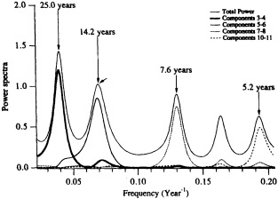
FIGURE 1
Stack spectrum of the central England temperature record, using SSA combined with a low-order, robust, maximum-entropy method. Each line shows the power spectrum of a particular oscillation, isolated as a pair of temporal EOFs, essentially removing the broad-band variability in which the peaks are embedded (see text for details). (From Plaut et al., 1995; reprinted with permission of the American Association for the Advancement of Science.)
from higher-frequency variability due to the El Niño/ Southern Oscillation phenomenon and volcanic eruptions. He emphasizes the need for using satellite data in considering spatial details of natural and anthropogenic variability, especially for temperatures aloft.
To derive full benefit from sophisticated methods of signal detection and analysis, the same methods have to be applied to the existing data and to model simulations. This emphasizes again the need for intercomparing detailed, but short, GCM simulations with the longer, but less detailed, time series generated by simple and intermediate models, as well as with the data themselves. These comparisons need to be carried out in both the spatial and the temporal domains.
A rich panoply of atmospheric models has been developed over the last 40 years, from zero-dimensional EBMs to fully three-dimensional GCMs, passing through one- and two-dimensional EBMs, RCMs, and dynamic flow models. These models have been widely used to study anthropogenic climate change due to increases in aerosol loading or greenhouse-gas concentrations. Their use for the study of internal climate variability on the time scales of interest here has only begun.
Understanding climate response to external forcing, natural or anthropogenic, requires that one understand slow shifts in equilibrium behavior, and then—more important—slow shifts in internal variability. Even for the former, passive response, considerable uncertainty exists at present as to amplitude and timing. The IPCC estimates the global surface air temperature increase for a doubling of present CO2 concentration to be anywhere from 1.5°C to 4.5°C
(IPCC, 1990); for a sudden doubling, decades to a century may elapse before a substantial fraction of this response will occur. The study of internal variability, and of its interaction with the external forcing, will require improving each type of model, and enhancing the intercomparisons between model results. A more intensive use of the hierarchical modeling concept can be guided by the ideas of nonlinear dynamics, which provide a common thread in the analysis of complex behavior for time-dependent models with arbitrary spatial detail.
Given the shortness of instrumental records, model validation on the decade-to-century time scale requires the use of sophisticated methods for their analysis and interpretation. A number of such methods have been applied recently to climate records, with promising results, and are being extended from the purely temporal to the combined space-time domain. These methods need to be refined further and applied systematically to model results, as well as to the existing records. Similar features detected in a consistent manner, by applying the same statistical methods, in models and data will increase our confidence in the former, our understanding of the latter, and hence our ability to predict climate change on the time scales of interest.
Modeling Low-Frequency Climate Variability: The Greenhouse Effect and the Interpretation of Paleoclimatic Data
TOM M.L. WIGLEY1 AND SARAH C.B. RAPER2
ABSTRACT
Detection of the decade-to-century time-scale effects of any external forcing agent on global-mean temperature requires a knowledge of internally generated natural variability on these time scales. Methods for estimating the magnitude of this variability are described. While the observed twentieth-century warming agrees well with model estimates based on greenhouse-gas and aerosol forcing alone, it is shown that changes of similar magnitude could have occurred solely through internally generated variability. Similarly, observed changes in global-mean temperature over the past 10,000 years (in particular, the numerous Little Ice Age events) could have been internally generated. At the very least, if these events were externally forced (e.g., by solar irradiance changes) then internal variability would probably have modified the response markedly from a "pure" response to external forcing, making the interpretation of the paleoclimatic record extremely difficult.
INTRODUCTION
Understanding the past is often said to be the key to predicting the future. The reverse is equally true: Attempts to predict the future can help us to understand the past. These maxims will be illustrated below.
An important but nebulous question raised in the context of the greenhouse effect is, "Have we detected it?" This issue concerns not just anthropogenic greenhouse-gas-induced climate change but past climate changes as well. The primary question in both cases is the identification of an externally forced change (a signal) in the presence of natural variability (background noise). Of course, detection requires more than just identifying a climate change that is consistent with some hypothesis—it requires also the demonstration of a cause-effect relationship and the attribution of some part of the observed changes to the particular cause. The present paper deals mainly with identification, rather than attribution.
We begin by comparing predicted and observed changes in global-mean temperature over the instrumental period, highlighting the role of low-frequency natural variability. We then review methods that may help to elucidate the character of this variability. Finally, we broaden the detection issue to consider the detection of external forcing effects
in general, and interpret the paleoclimatic record in this general detection context. The key distinction here is between externally forced and internally generated low-frequency natural variability. Separating these factors in past data appears to be a very difficult task.
CLIMATE CHANGE SINCE PRE-INDUSTRIAL TIMES
The most obvious detection-related question is: Do the observed changes in global-mean temperature agree with predictions of changes induced by human activities? To answer this question we need an estimate of the predicted changes (the signal), appropriate observational data, and suitable statistical methods to compare the two—i.e., to decide whether any similarity between them is more than might be expected to occur by chance. The last aspect requires a knowledge of the low-frequency character of natural climate variability.
The anthropogenic global-mean temperature signal to date (1765-1990) is subject to considerable uncertainty. Predictions of this signal depend both on the radiative forcing changes that have occurred and on how temperature responds to such changes (which, in turn, is determined largely by the climate sensitivity). Both factors introduce uncertainties. The imposed forcing, while undeniably large, is uncertain by a factor of two (1.06 to 2.06 W m-2, global-mean). Following Wigley and Raper (1992), the total forcing may be broken down into the effects of CO2 (1.50 W m-2), CH4 (0.56 W m-2), N2O (0.10 W m-2), halocarbons (0.02 to 0.28 W m-2, depending on whether one includes the possible effect of halocarbon-induced stratospheric ozone changes), and SO2 -derived sulphate aerosols (-0.38 to -1.13 W m-2).
Most of the forcing uncertainty derives from the aerosol component. The lower limit for the total global forcing, about 1 W m-2, corresponds to the high aerosol forcing case. While the magnitude of the aerosol forcing is highly uncertain, its upper bound is probably constrained by observational evidence of hemispheric-scale temperature changes. Because most of the forcing is in the Northern Hemisphere, a global-mean aerosol forcing in excess of about -1 W m-2 would imply such a large interhemispheric forcing contrast3 that the effects would likely be obvious in the observed temperature data (Wigley, 1989).
The response to this man-made forcing, i.e., the global-mean temperature signal, is subject to still further uncertainties. These arise mainly from uncertainties in the climate sensitivity and in the damping effect of oceanic thermal inertia. For "best-guess" forcing (1.44 W m-2 over 17651990), simple model calculations (using an energy-balance model with an upwelling-diffusion ocean) give a warming over 1880-1990 of 0.3 to 0.6°C (corresponding to a climate sensitivity of 1.5 to 4.5°C for 2 × CO2) (Wigley and Raper, 1992). The range of possible values is slightly increased if one accounts for uncertainties in the model parameters that determine ocean mixing, and is considerably larger if one accounts for forcing uncertainties.
The above model-based range for 1880-1990 warming is, in fact, the same as the range that the Intergovernmental Panel on Climatic Change (Folland et al., 1990) gives for the observed warming over this period. What is the significance of this consistency? From paleoclimatic data, we know that the climate system has a high level of natural variability. A greenhouse-warming skeptic could claim, therefore, that the observed warming was merely (or largely) natural variability, that the consistency was a fluke, and that the model-predicted warming was too high. Alternatively, greenhouse-warming extremists might claim that the model prediction was too low, and that natural variability had actually offset a much larger anthropogenic signal. Clearly, a crucial issue is to unravel the effects of man from natural variability on the time scale of 50 years or more. Unfortunately, our quantitative knowledge of natural variability is at least as poor as our knowledge of the enhanced greenhouse effect. Furthermore, as we will show below, the magnitudes of any externally forced temperature signal and of low-frequency internal variability are both dependent on the climate sensitivity, making their separation even more difficult.
QUANTIFYING LOW-FREQUENCY VARIABILITY
How do we obtain information about natural 50-year time scale fluctuations in annual global-mean temperature? There are two possible approaches: using observational data, or using models.
Using Observational Data
If observational data are to be used directly, then one must resort to paleoclimatic data because of the limited duration of the available instrumental record. Paleoclimatic information, however, is invariably local or regional rather than global, and the data are usually seasonally specific and subject to uncertainties because of the complex links between proxy data and temperature (see, e.g., Bradley and Jones, 1992a). It is therefore very difficult to estimate changes in annual global-mean temperature prior to 1860.
In spite of the data uncertainties, there is strong evidence that substantial 50-year time-scale changes in global-mean
temperature have occurred over the past 10,000 years (i.e., the period over which we have the best data and during which the planet's albedo-related boundary conditions have probably varied little) (Röthlisberger, 1986; Grove, 1988). Since this evidence is indirect and based on limited geographical coverage, we can only offer speculative estimates of the magnitude of these annual global-mean temperature changes. Most probably, the fluctuations have been within a band 0.5°C wide (Wigley and Kelly, 1990). Dating and data uncertainties do not allow us to compare the recent warming with similar warmings in the past in any useful quantitative way, so we cannot say whether the twentieth-century warming is occurring at an unprecedented rate.
Using Models
An alternative approach is to try to estimate 50-year time-scale variability using either a statistical or a deterministic model. In both cases, information from the observed, instrumental record of global-mean temperature changes over the past 130 years is used to estimate the spectrum of natural variability over the full range of frequencies.
In the statistical approach, the data are fitted to a standard-time series model of some sort (such as an nth-order autoregressive process or some more complex model), and the fitted model is used to extend the spectrum to lower frequencies (e.g., Bloomfield and Nychka, 1992; Kheshgi and White, 1993).
A deterministic approach has been used by Wigley and Raper (1990, 1991). Here, a simple climate model is employed to extend the spectrum of observed variability: The method used is to force the model stochastically with white-noise forcing, the magnitude of which is chosen to match the observed high-frequency variability (1- to 10-year time-scale). It should be noted that this approach yields information only on passive internal variability, i.e., variability that arises in the absence of ocean circulation changes. Low-frequency variability may also occur, for example, through changes in the ocean's thermohaline circulation, as evidenced by recent coupled ocean/atmosphere general-circulation model (GCM) results (e.g., Washington and Meehl, 1989; Manabe et al., 1991; Cubasch et al., 1992) and by much longer simulations with an ocean GCM (Mikolajewicz and Maier-Reimer, 1990) and with a two-dimensional ocean model (Mysak et al., 1993). It has been speculated that such circulation changes may be coupled to surface temperature changes, leading to feedbacks that would amplify low-frequency climate variability (e.g., Gaffin et al., 1986; Piehler and Bach, 1992; Harvey, 1992). Model simulations of passive internal variability, therefore, may only represent a lower bound to overall internally generated variability.
An example of the output from a simulation of passive internal variability is given in Figure 1. For a simple linear first-order model (e.g., a one-box ocean model) white-noise forcing as input is transformed to red-noise temperature output, with an enhancement of variability at low frequencies. For more complex models (such as that used here), the output spectrum is still basically reddish in character, in that there is a marked enhancement of the power at low frequencies.
The passive internal variability modeling approach gives results very similar to those of the statistical model of a fractionally integrated white-noise process that is preferred by Bloomfield and Nychka (1992) (see Figure 2). The deterministic modeling approach yields additional physical insights. It shows that high-frequency variability (≤ 10 years) is virtually independent of the climate sensitivity (ΔT2×), and mainly reflects the magnitude of the forcing and the heat capacity of the upper mixed layer of the ocean (Wigley and Raper, 1991). For similar reasons, the response to short-lived forcing events, such as those of volcanic eruptions, is also independent of ΔT2×. This is why interannual variability can tell us nothing directly about ΔT2×. At low frequencies (≥ 30 years), however, the temperature-response spectrum of passive internal variability depends critically on ΔT2×.
If we had evidence of large natural climate excursions in the past on the 50-year time scale, there would be two
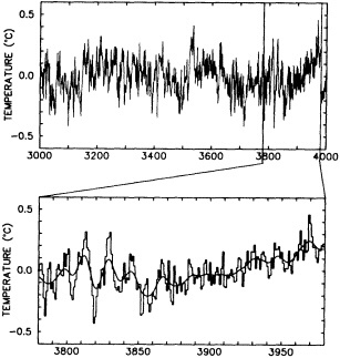
FIGURE 1
A simulation of internally generated natural variability of global-mean temperature (using ΔT2× = 2.5°C). The upper panel shows the third 1,000 years of a 100,000-year run; the lower panel shows an enlargement of 200 years of this record. (From Wigley and Raper, 1991; reprinted with permission of Elsevier Science Publishers BV.)

FIGURE 2
Spectral densities for observed and simulated global-mean temperature series. Items 1 to 4 are spectra of the observed data based on different assumptions regarding the underlying statistical structure of the data. Item 5 is a theoretical response spectrum for white-noise forcing derived from a global upwelling-diffusion energy-balance climate model. Item 6 is the spectrum based on data from a more complex form of the same model forced with white noise. (From Bloomfield and Nychka, 1992; reprinted with permission of Kluwer Academic Publishers.)
possible interpretations. First, if the climate sensitivity were low, then passive internal variability and any response to global-mean external forcing would be small, so we would have to invoke either significant changes in the thermohaline circulation or (less likely on these time scales) major changes in the spatial patterns of forcing (as in the Milankovitch effect). Alternatively, if neither of the latter two mechanisms was operating, we would have to infer that the climate sensitivity was relatively large (i.e., ΔT2× in the range suggested by GCMs, 1.5°C to 4.5°C), since a large sensitivity is required for both passive internal and global-mean externally forced changes to be substantial.
The Importance of Climate Sensitivity
In the following, we assume that the climate sensitivity lies in the commonly accepted range of 1.5°C to 4.5°C, and consider some of the consequences. The dependence of passive low-frequency variability in global-mean temperature on ΔT2× has two important implications. First, as noted earlier, it means that the problem of separating a low-frequency (e.g., greenhouse) signal from low-frequency natural variability is one that is with us no matter what the value of ΔT2×; both signal and noise increase as ΔT2× increases. On the other hand, the dependence of low-frequency variability on ΔT2× gives us the possibility of estimating ΔT2× from the spectral character of the past (paleoclimatic) climate record. Unfortunately, as noted above, our quantitative knowledge of this past record is poor, so we cannot use it to derive any reliable information regarding ΔT2× , at least on the basis of recent (the past 10,000 years) paleoclimatic data. Attempts have been made, however, to use longer-time-scale paleoclimatic data. These point to ΔT2× being around 2.5°C, but with a range of uncertainty similar to that deduced from GCMs (see, for example, the recent work by Hoffert and Covey, 1992).
The deterministic modeling approach can also be used to estimate statistical confidence limits on natural century-time-scale trends in global-mean temperature. The results, which depend on ΔT2×, show that a trend of more than 0.3°C per century is unlikely (95 percent confidence level) on the basis of passive internal variability alone. Since other forms of natural variability exist (due to external forcings at low frequencies, or due to ocean circulation changes), a natural trend of about 0.5°C per century is certainly possible, although such a natural trend is as likely to be negative as positive.
Both external forcings (man-made and/or natural) and internally generated variability could have contributed noticeably to the twentieth-century trend. The relative importance of these factors over this period is uncertain. Nevertheless, we can infer from the very existence of the trend that ΔT2× must be far from negligible. Given that there is no evidence of thermohaline circulation changes large enough to cause such a large overall trend (see, e.g., Wigley and Raper, 1987), a substantial climate sensitivity is necessary no matter what the cause of the trend. External forcing can clearly have a marked response only if ΔT2× is substantial. For example, if man-made forcing were the major factor, then ΔT2× would have to be 2°C or more (Wigley and Raper, 1992). For passive internal variability to contribute substantially to the trend, ΔT2× must also be of similar magnitude (Wigley and Raper, 1990). Thus, although we cannot claim to have detected the enhanced greenhouse effect on the basis of the data alone (note the conditional clause), the data do give us valuable insights into the way the climate system works.
INTERPRETING THE PALEOCLIMATIC RECORD
Detecting the enhanced greenhouse effect has a strong parallel in trying to interpret the paleoclimatic record. One of the justifications commonly used for work in paleoclimatology is that the data can provide information on the causes of past climate change. At least for the past 10,000 years, however, identifying causes, or even distinguishing exter-
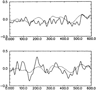
FIGURE 3
Two contrasting simulations of global-mean temperature changes over A.D. 0 to A.D. 600. During this period, the forcing shows noticeable but relatively weak fluctuations (range about 0.5 W m−2). In the upper simulation, the ''observed" (signal plus noise) temperature fluctuations (full line) bear no resemblance to the signal (dashed line). Temperatures remain roughly constant over A.D. 0 to A.D. 500 and then rise rapidly by about 0.3°C over about 10 years, but this rise is unrelated to the forcing. In the lower panel, there are major fluctuations of magnitude far exceeding the largest of the fluctuations in the signal. The rapid cooling over A.D. 100 to A.D. 140 is followed by an even larger warming (0.7°C over A.D. 140 to A.D. 200) and a subsequent long-term cooling trend over A.D. 200 to A.D. 420. None of these events is a reflection of the forcing changes.
nally forced as opposed to stochastically forced events, could be difficult. The reason for this is that the potential magnitude of internal variability, as revealed by the modeling work described above, is similar to the range of observed changes over the past 10,000 years. Thus, even if the major climate excursions of the past (such as the Little Ice Age) were externally forced, internal variability may mask these to such an extent as to make their interpretation problematic.
To demonstrate this, we use the last 2,000 years of a hypothesized record of past external (solar) forcing derived from radiocarbon data from precisely dated tree-ring samples (from Stuiver and Braziunas, 1989). The magnitude of this forcing is uncertain, so we choose the scale to give a range of modeled global-mean temperature changes of 0.5°C for ΔT2× = 2.5°C. (The corresponding forcing range is about 1 W m−2, similar to the magnitude of man-made forcing over the past few centuries.) To simulate internally generated natural variability, we superimpose on this solar forcing record additional white-noise forcing. The magnitude of the white-noise forcing is chosen so that the high-frequency (≤ 10 years) variability of the modeled temperature changes matches that of the twentieth-century temperature data. This produces a low-frequency internal variability background whose magnitude depends on ΔT2×.
Even though both the response to external forcing (i.e., the signal) and the magnitude of passive internal variability (i.e., the noise) depend on ΔT2×, this does not necessarily mean that the signal-to-noise ratio in our simulations is independent of ΔT2×. If we were to keep the externally forced range of temperature changes at 0.5°C (to do this, we would have to assume larger solar forcing if we used a smaller ΔT2×), then the signal would stay constant, but the noise would vary with ΔT2×. If, however, we kept the forcing fixed, then the relative magnitude of signal to noise would be effectively independent of ΔT2× (in this case, lower ΔT2× would lead to a lower externally forced range and a similarly reduced internal variability range). It is not clear which would be the better approach. We avoid the dilemma by considering results for only a single value of ΔT2× (2.5°C); this is all that is required to illustrate the problem of interpreting the past record.
Figures 3 and 4 give selected examples showing the combined externally forced and internally generated variations in annual global-mean temperature compared with the
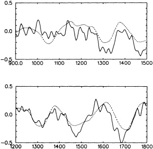
FIGURE 4
In the upper panel, the cooling event evident in the signal around A.D. 1000 to 1100 (dashed line) is entirely absent from the simulated record, while the subsequent two forced cooling events around A.D. 1300 and A.D. 1500 show up quite clearly. In the lower panel, there are three cooling signals (A.D. 1300, 1500, and 1700), all of which show up in the simulated observed record. In the last event, however, the observed cooling leads that in the signal by 20 to 50 years. The strength of the signal in all three events is similar, but the realized magnitude differs markedly.
externally forced component alone. (Note that these are not necessarily typical examples—they represent cases that might be expected to occur about 10 percent of the time). In many instances, there are marked differences between signal and signal-plus-noise. For example, even when the external forcing component is small, warm and cold intervals may occur that are as large as many of the major externally forced episodes; external forcing effects are often masked by internal variability; and noticeable "phase shifts" occur in which the "observed" (signal-plus-noise) changes appear to lead the forcing by a number of decades.
What does this mean for interpretation of the observed paleoclimatic record? For these data, we only have a single manifestation of an ensemble of internally generated possibilities. Since signals and (passive) noise can be of similar magnitude (albeit with relatively low probability), it would be possible to completely misinterpret the observed record even if it were perfect (i.e., a faithful representation of annual, global-mean temperature changes). It should not be surprising, therefore, that attempts to associate cause and effect in the paleoclimatic record have invariably met with only limited success (see, e.g., Wigley and Kelly, 1990). Even with perfect forcing and response data, we would not expect to get highly significant results when comparing theory with observations.
This brings us back to our initial statement. It would indeed be useful to understand the causes of past climate change, but we are unlikely to unravel this puzzle easily. At least for the past 10,000 years, the forcing (as deduced from a noise-free interpretation of observed data) is such that signal and noise may be of similar magnitude. Anthropogenic forcing over the past few centuries has almost certainly been larger in magnitude than any natural forcing that has occurred at the annual, global-mean level. Thus, detection of the enhanced greenhouse effect (given that we are still enhancing it!) is probably an easier task than explaining the past, and efforts to improve future climate predictions are likely to add more to our understanding of the past than vice versa.
Discussion
LINDZEN: I'd like to comment on something common to Jerry North's and Tom Wigley's papers. Both use very simple models, which I myself favor. But because of this simplicity, they can be forced only in a certain way, and they also lack the feedback that is one of the determinants of the delay imposed by the ocean's heat capacity. The latter must be kept in mind in the interpretation of such models' results.
ROOTH: I consider it a serious flaw that these models treat the ocean in such a lumped way as regards delay effects. When you change surface temperature by a couple of degrees, you want to have a proportional change decaying toward deep water.
NORTH: I want to make it clear that the Wigley-Raper model and the one I talked about are exactly the same, except that ours has geography. Now about the delay: Last year we did a little study of the ramp warming with that model, and found that it matters very much when you start the ramp. Two times are very important: One is how long it takes for the model to adjust to the linear ramp, and the other is the delay. The delay is frequently a few decades, in our models as well as the coupled GCMs, but the adjustment time seems to be extremely model dependent. In these simple models it can be 150 years or so, which limits the warming you can have, whereas the GCMs get onto the ramp so quickly it's hard to get slow warming. I don't know the answer to this dilemma.
[UNKNOWN]: One crucial thing we don't know from the data is the natural relaxation time. A shoulder you see on some of these power spectra, between a flat spectrum to the left and a slope to the right, is occurring effectively at 10 years. If this break in the slope is an empirical measurement of a response time, that has important implications.
LINDZEN: We must be careful not to construe model spin-up as a characteristic delay.
MYSAK: I just wanted to agree with Claes about ocean response to SST changes, and to say that I think we have learned a lot about the natural variability of the ocean's thermohaline circulation in the last few years. Modeling work at several places has shown natural oscillations in the range of 100 to 300 years.
GHIL: It seems to me that we have a spectrum of more or less predictable types of climatic behavior that ranges from totally boring to completely surprising. We go from a predictable trend through periodic, quasi-periodic, and deterministically aperiodic behavior all the way to random noise. Natural variability is the sum of all these things, and we need methods that can distinguish among them.
Detection of Forced Climate Signals
GERALD R. NORTH AND KWANG-YUL KIM1
ABSTRACT
A method of signal detection used in communication theory can be applied to the problem of detecting forced climate signals. This method calls for the construction of an optimal filter (averaging procedure) which is then applied to a data stream that varies in both space and time such that the natural variability is suppressed to the maximum extent possible. The construction of such filters requires a good knowledge of the waveform of the signal and the frequency-dependent empirical orthogonal functions for the natural variability. Although we cannot yet supply reliable estimates of either of these from data or from coupled general-circulation-model simulations, we present some samples that are based on simple stochastic models. These exercises suggest that the signal due to sunspot forcing, while quite weak, can be considerably enhanced by using optimal filters. Greenhouse warming, modeled with a ramp increase of temperature, presents a large signal-to-noise ratio. Either the observed warming signal is highly significant, or the surface climate has experienced a very rare natural fluctuation over the last century.
INTRODUCTION
To detect a faint signal that is superimposed on random fluctuations, it is helpful to know as much as possible about the characteristics of the fluctuations and the form of the signal. In the detection and attribution of forced climate signals we are faced with this generic problem. But precisely in what form do we need variability statistics? And how can we objectively employ variability statistics in our detection strategy? Can sensible statistical tests be applied using this information? Is there an optimal procedure that will assist us in formulating our questions clearly? Some of the answers lie in a class of techniques known to signal-processing engineers for over half a century, dating to the work of Wiener (e.g., as summarized in his 1949 book) and Kolmogorov (1941). Such techniques were first connected with the climate problem by Hasselmann (1979) and Bell (1982, 1986). Other approaches to the climate-change detection problem have been taken by Barnett and colleagues (e.g., Barnett, 1986, 1991). Several others are summarized in a recent book edited by Schlesinger (1991). Here I summarize the signal-processing approach as detailed by North et al. (1992).
Our goal is to develop a filter (a weighted averaging process) that can be applied to the historical data stream in space and time so that the signal or "forced part" of the stream is optimally enhanced by comparison with the natural variability or "noise." By a filter we mean a linear operation on the data stream such as a weighted integral over the globe and over the past. This space- and time-dependent weighting function essentially constitutes a filter. This function must take place despite an imperfect observing system and an imperfect knowledge of the signal. To pose the problem formally, we seek a filter that minimizes the mean squared error between our estimator for the signal and the true signal. Implicit is the assumption that the data stream Tdata(r,t) can be written as a sum of signal and noise parts,
where TS(r,t) is the forced signal and TN(r,t) is the natural variability.
This assumption has been shown to be adequate for a general-circulation-model (GCM) simulation of the surface temperature field for an idealized planet (North et al., 1992). We conjecture that it holds for the more general questions of interest, but it is particularly problematic for studies of the world ocean. The mathematical expression for a filtered data stream, ![]() is
is
where D is the spatial domain and G(r,t;r',t') is the filter kernel.
AN EXAMPLE
Consider a planet that experiences periodic (forced) solar luminosity. Simulations of climate indicate that the resulting spectrum of the global average temperature contains a simple red-noise continuum with a sharp peak at the forcing frequency (North et al., 1992), provided the thermal response amplitude is no more than a few degrees. If we know the imposed forcing and response frequency from theory, we can filter the data stream so that only a narrow band of frequencies around the peak is retained. The longer the time series of data, the narrower can be the filter.
Much more can be done if the temporal profile (waveform) being detected is known precisely. In the case of the oscillating solar luminosity, for example, the phase of the imposed sinusoid is known as well as the frequency. Since the noise is independently distributed between sine and cosine components, we can further select within the frequency band to eliminate phases that are unlike the signal. For example, if the signal is all sine component, we can eliminate the cosine component with a simple projection filter. Since the random-noise component for a stationary process distributes variance equally between the sine and cosine components, we can reduce the variance of the noise by a further factor of two, or reduce the noise standard deviation by the square root of two. In this way we can hope to increase the signal-to-noise ratio considerably more than can be accomplished with a simple frequency band-pass filter.
In fact, there is even more enhancement potential at our disposal. If the forced response has a characteristic geographical signature at the responding frequency, we can use our filter to select only geographically similar patterns. This procedure can be employed to eliminate any patterns occurring in the natural variability that are dissimilar (orthogonal) to the signal pattern. It follows that very faint signals can be seen if we know enough about them a priori and if enough of the noise is orthogonal to the signal. Our experimentation with stochastic energy-balance models suggests that at least another factor of two in the signal-to-noise ratio can be gained from this extension to pattern recognition.
While the sinusoidal example is interesting, and potentially useful for the important sunspot-response detection problem (it is important mainly because it may tell us something about climate sensitivity at the decadal-scale), it is more idealized (being nearly a sharp tone) than the one we face in the greenhouse problem, which is spread over a broad continuum of frequencies.
In contrast to the periodically forced system, the greenhouse problem presents a single ramp-like waveform with a characteristic geographical response pattern (land-surface temperatures tend to lead slightly over ocean-surface temperatures). Hence, the response will be composed of a large number of sinusoidal frequencies in the Fourier sense. Since the pattern of response of the surface-temperature field depends strongly on the forcing frequency, we will find it natural to use frequency-dependent empirical orthogonal functions (fdEOFs) as an expansion basis (see, e.g., North, 1984). We stress that this is not just a convenient choice, but one that arises naturally from the formalism as the optimum for such purposes.
MEAN-SQUARE-ERROR FORMALISM
In this section we formulate the mean square error (MSE) for the random component of the error made with our estimator of the signal for a given realization. Unfortunately, in the climate problem we have only one realization to work with. In this paper we dispense with mathematical detail, referring the reader to the paper by North et al. (1995) for detailed derivations. The error in question is the difference for an individual realization between the estimator of the signal (filtered data stream) and the actual signal, whose shape in space and time must be known a priori. We form the square of this error and average it over an ensemble of realizations of the same waveform embedded in natural
variability. The natural variability is uncorrelated from one realization to another. The geographical dependence of the natural fluctuations will be taken to be stationary in time. The mathematical expression for the MSE is
After formulating the expression for the MSE, we find that it can be written in terms of a weighted space and time integral over the unknown filter. If we take the variation of the MSE with respect to infinitesimal changes in the unknown filter function in space and time and set the resulting expression equal to zero, we end up with an integral equation for which the filter is the unknown. An important special case is that for which a no-bias constraint is imposed. We would like to make our estimator of the signal be unbiased. For this case, the ensemble average of the filtered data stream is identical to the true signal except that it is multiplied by a constant factor that is realization dependent. The constraint can be incorporated by the use of the familiar method of Lagrange multipliers. The result is again an integral equation that has to be solved for the optimal filter as its unknown,
where ρ(r,t;r',t') is equal to ![]() and Λ is the Lagrange multiplier.
and Λ is the Lagrange multiplier.
OPTIMAL-FILTER SOLUTION
The integral equation for the optimal filter is a simple nonhomogeneous linear integral equation, in which the desired filter function occurs under the integral sign, weighted by a kernel. The kernel of the integral equation happens to be the space-time lagged covariance of the field in question (e.g., the surface temperature field). This tells us that the optimal filter is strongly dependent on the structure of the space-time covariance of the natural variability. In addition, the optimal filter depends on the signal itself. Later we will discuss solutions for which there is some uncertainty in the signal (as actually occurs).
In solving a linear integral equation in which the unknown occurs underneath the integral sign, weighted by a kernel that is symmetric in its arguments (e.g., a covariance), it is advantageous to expand the kernel into its eigenfunctions. Since the kernel is symmetric and well behaved, we can assume the eigenfunctions form a complete basis set with positive eigenvalues that satisfy
where Ψn(r,t) is the frequency-dependent EOF and λn is the eigenvalue. The eigenfunctions of a covariance kernel are known as the empirical orthogonal functions (EOFs). The eigenvalues are the variance attributable to the corresponding EOF "mode." We can reduce the integral equation to so-called diagonal form by expanding all quantities in terms of the eigenfunctions of the kernel. This is equivalent to inverting a matrix by using a basis in which the matrix is diagonal, which simply requires inverting the elements along the diagonal.
Since the natural variability can be taken to be stationary in time, the temporal part of the problem can be solved using the Fourier (integral) basis. The spatial part of the problem is solved at each frequency by using the EOF basis set for that frequency. The choice of frequency-dependent EOFs completely diagonalizes the space- and time-dependent kernel of the integral equation, rendering the problem invertible. Hence, the problem of constructing an optimal filter amounts to obtaining an adequate knowledge of the fdEOFs and an a priori knowledge of the signal shape in space and time. In principle, each could be obtained from simulations with sufficiently reliable coupled ocean-atmosphere climate models.
The signal waveform in space and time and the data stream are to be expanded into the frequency-dependent EOF basis set. After the insertion of these into the integral equation, we find the following formula for the optimal filter:
PROPERTIES OF THE OPTIMAL FILTER
The unbiased optimal filter for a known non-random signal turns out to be exactly proportional to the known signal waveform. This space-and time-dependent shape factor can be moved outside the integral sign when the data are filtered (see equations (2) and (6)). The filtered data stream then is the imposed signal, as a function of space and time, multiplied by a realization-dependent dimensionless scale factor whose expectation value is unity. The signal-to-noise ratio is the reciprocal of the standard deviation of the scale factor. This standard deviation is a key property of the optimal filter. The square of the signal-to-noise ratio can be written as a sum of terms, each of which represents the contribution from a particular fdEOF mode:
This representation is particularly convenient, since it allows us to see how adding more modes in the expansion affects the performance of the filter. A filter in which the series is
truncated is an unbiased suboptimal approximation to the optimal filter.
Each term in the sum for the signal-to-noise ratio squared is the ratio of the square of the signal projected onto mode n divided by the fdEOF eigenvalue corresponding to that mode (7). Hence, each term can be interpreted as the ratio of the square of the signal amplitude to the noise variance for that mode. If the signal is confined to only a few fdEOF modes, the sum will terminate quickly. If it is broad-band, the sum will have many terms, each one of which is positive. A highly desirable situation is one in which the signal projections are large, for modes with small eigenvalues. Clearly, it is important to estimate the rough size of the signal-to-noise calculation before performing any data manipulation or extensive model simulations, since detection of the forced signal may be impossibly difficult even with an optimal filter.
PILOT MODELS FOR CLIMATE SIGNAL DETECTION
Energy-balance models (EBMs) have proven to be able to simulate the geographical distribution of the seasonal cycle of surface temperature (North et al., 1983; Hyde et al., 1989). When EBMs are forced with white noise (in space and time), they have also been shown to reproduce the geographical distribution of the variance of natural fluctuations in frequency bands from two months to a few years (Kim and North, 1991). Even the geographic distributions of spatial correlation characteristics from EBMs are in good agreement with observational data for these same frequency bands. The only new parameter in the noise-forced simulations is the strength of the noise forcing. Even this cancels out in the computation of correlations. Such a forced model enables us to compute the fdEOFs exactly. We dub them frequency-dependent theoretical orthogonal functions (fdTOFs), since they come from a theoretical model rather than from data. When we computed these fdTOFs and compared them to those computed from 40 years of surface-temperature data, they were in reasonable agreement (Kim and North, 1993).
We have extended the noise-forced EBMs (nfEBMs) to include a deep ocean similar to that used in a number of studies by the IPCC (IPCC, 1992; see also Hoffert et al., 1980). The model consists of land and ocean distributed on the globe's surface. The ocean consists of a mixed layer of 75 m depth atop a deep ocean, which transports heat by way of uniform upwelling and uniform thermal diffusion. Such an ocean model develops a thermocline at a depth of about 1 km for a reasonable choice of the two new parameters (Kim et al., 1992). The new coupled model still reproduces a good seasonal cycle and second-moment variance and covariance characteristics. Its lower-frequency behavior is thought to be somewhat improved over that of the earlier mixed-layer-only version (Kim and North, 1992).
The new coupled (linear) model is capable of producing fdTOFs for the natural-variability and forced-climate signals. The static sensitivity of the model is somewhat low as climate models go: 2°C for a doubling of carbon dioxide and 1.2°C for a 1 percent increase in solar constant. These last quantities do not depend on the ocean, since they are static (for transition from equilibrium to equilibrium) characteristics. The transient behavior of the model is fairly well understood. For a ramp in greenhouse forcing starting in the year 1750, the model produces about a 0.5°C increase over the last century. One important signature or fingerprint of this type of forcing is that the mid-Asia minus mid-Pacific differences over the last century are about 0.13°C. Hence, in this class of models there is a potentially significant land-sea contrast in the warming that can be exploited for pattern recognition. In greenhouse warming, land leads ocean by a potentially detectable amount. If warming is caused by internal variability of the oceans, we would expect ocean to be leading.
Next we consider a few explicit numerical examples in which the signals and noise are computed from nfEBMs (e.g., Kim and North, 1992; Kim et al., 1992).
SUNSPOT EXAMPLE
We have measurements of the solar constant taken from several independent satellites over the last 12 years. There
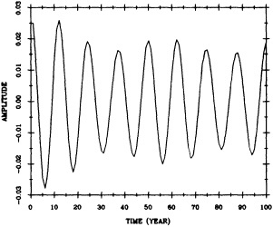
FIGURE 1
Response over the last century of the globally averaged temperature to sunspot-cycle forcing as computed by the Kim-North-Huang (1992) model. The variation of sunspot number is converted to a variation in solar constant using the last solar cycle. The Kim-North-Huang model is an energy-balance model of the surface temperature over land and the mixed-layer temperature over ocean atop an upwelling-diffusion deep ocean.
does appear to be a small oscillation of the solar constant that is consistent with a modulation by the sunspot number. The amplitude of the oscillation appears to be about 0.1 percent. If we use this one cycle as a calibrator and ask what the temporal variation over the last century would have been, we can proceed to compute the climatic response of the earth. Figure 1 shows the curve of the global average temperature as computed by the Kim-North-Huang model. The response is a disturbed 11-year cycle with an amplitude of about 0.02°C, a very faint signal considering that the standard deviation of one-year averages for natural variations is about 10 times larger. This simple exercise suggests a signal-to-noise ratio of about 0.1, implying that the signal is virtually undetectable. On the other hand, if we use more information, which is fortunately at our disposal (at least from the model simulations), we can do much better.
Next we show the results of optimal filtering of the data to detect the surface-temperature response to the sunspot cycle. Figure 2 shows the geographical pattern of response to an 11-year periodic solar forcing in this model. When this pattern is included along with the precise phase and amplitude information represented in Figure 2, the signal-to-noise ratio squared can be plotted as a function of the number of fdTOFs included as shown in Figure 3. A monotonic increase in the signal-to-noise ratio can be seen as more fdTOFs are included. Hence, we have shown that the method is capable of improving signal-to-noise ratio through
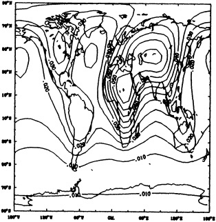
FIGURE 2
Geographical signature of the amplitude of the surface-temperature response for solar-constant oscillations of 0.1 percent at a period of 11 years, as computed in the Kim-North- Huang model.
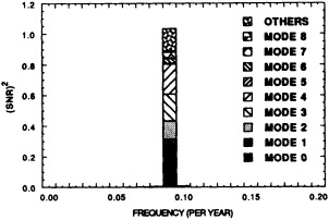
FIGURE 3
Theoretical signal-to-noise ratio squared for the sunspot-forcing problem. The bar graph shows contributions from different frequencies. Within each bar is the partitioning of contributions from different spatial EOFs at that frequency. One sees that the contribution from spatial-pattern recognition is significant.
the inclusion of geographical, frequency, and phase information in the filter. The signal-to-noise value of the order of unity is still short of acceptable for purposes of detection, but the sunspot cycle is used here mainly for illustration (although we think more can be done with the sunspot problem). Significant degradation will occur when we start to use real data instead of simulated data.
GREENHOUSE-WARMING DETECTION
Confirming the existence of greenhouse warming consists of detecting a ramp-like increase of temperature over the last century. Our simulations show that the differences between the 1980 and the 1880 surface temperature fields should look like the map shown in Figure 4, which clearly shows the land-leading effect. If we expand our ramp-like response into sine and cosine harmonics of 100 years and into the fdEOFs at these frequencies, we can estimate the signal-to-noise ratio squared, as we did in the sunspot case. The result is shown in Figure 5. We find that greenhouse-warming detection is not helped as much by the addition of pattern recognition as sunspot-cycle detection, but the signal is large enough to be detected with considerable confidence. Thus, if our assessment of the low-frequency variance in the model is correct, either the greenhouse-warming ramp is real, or a very rare natural fluctuation with a positive slope of 0.5°C per century is occurring. (By a rare natural fluctuation we mean one that is 0.25°C above normal and lasts for a century.)
CONCLUSIONS
Signal-processing methods can significantly enhance our ability to detect forced climate response. It is important to
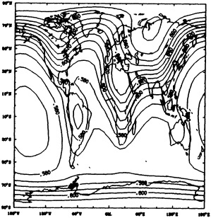
FIGURE 4
Temperature-difference map for 1980 to 1890, as computed by the Kim-North-Huang model.
note that the word "detect" can be misleading. We do not mean that we show that such a signal is present or not present. Our procedure aims to measure the strength of the signal, given its waveform in space and time. We need a good model of the signal beforehand, and we need a good understanding of the lagged covariances so that we can compute the fdEOFs—or more likely the fdTOFs, since long enough strings of data will not be available. It is especially important to have good low-frequency fdTOFs. Once these quantities are in place, we can construct an optimal filter for the data stream. It is possible to relax some of these requirements, such as the need to have perfect knowledge of the signal. We may know only its probability distribution, for example. This kind of statistical information can also be used to construct an optimal filter at the cost of some reduction of the signal-to-noise ratio.
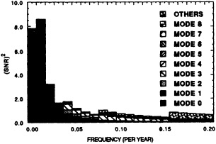
FIGURE 5
The square of the theoretical signal-to-noise ratio, as in Figure 3, for the greenhouse-warming problem. The signal is a (repeating) ramp upward of 100 years' duration.
We feel that it will be possible to use the techniques just mentioned to construct filters capable of achieving a signal-to-noise ratio greater than 10 for simulated data. Moving to the inclusion of real data is a large leap, however. First, the actual data are imperfect, coming as they do from a sparse network that is itself time dependent. The effects of variations in the observational network can be included in the filter formalism, and we intend to test some of them in the near future. Second, we lack complete knowledge of the signal. We hope to show the consequences of poor signal knowledge through modeled examples in future papers.
Finally, it must be re-emphasized that our method depends on the assumption that signals (whose waveform is calculable a priori) and stationary random fluctuations can be linearly separated. These components do not depend upon each other in our formulation. It is likely that none of these assumptions holds strictly for the climate system, but it would seem unwise to take a more complicated approach until the proposed one has been demonstrated to fail.
Discussion
GHIL: Aren't you actually trying to distinguish between two kinds of signal, one anthropogenic and one that could be called a deterministic part of natural variability? It seems to me, furthermore, that singular spectrum analysis, which is a data-adaptive version of the Wiener-Kolmogorov filter, does some of the same things rather better. Myles Allen at Oxford has developed a test like the one Dick Lindzen wants, and when he applied it to a long time series for central England he got interdecadal natural-variability peaks.
NORTH: Perhaps I didn't explain carefully enough that I have termed the natural variability "noise" with respect to the anthropogenic "signal". Also, I see no reason to adopt fancy techniques to deal with a stationary time series.
LINDZEN: I think we need to address the physics of these primitive models you and Tom Wigley have used, which have a forcing function that pulses.
MOREL: I recently had the opportunity to see the results obtained by the Hamburg group. They have run four different globalwarming experiments at 30-year intervals, with widely differing responses. In fact, their warming curves are so different it is impossible to distinguish between variability and warming.
NORTH: Our empirical orthogonal functions suggest that we have nailed down the eigenvalue spectrum extremely well. Also, when we used the model on the NCAR data set, we found that the pattern of variance was totally dominated by the land-sea contrast. At lower frequencies the El Niño signal begins to appear, which seems to me to be a good indicator of usefulness.
Constraining Possibilities Versus Signal Detection
RICHARD S. LINDZEN1
ABSTRACT
Rather than concentrate on the problem of greenhouse signal detection, one can exploit the intimate relation of climate sensitivity to length of ocean delay in order to constrain possibilities. It is noted that the observed record of surface temperature is "broadly" consistent with equilibrium sensitivity to CO2 doubling of between 0°C and 4.8°C—provided that the ocean delay for the higher sensitivity is of the order of 160 years. If ocean delay can be independently established as being shorter, then one must reduce the maximum consistent sensitivity. It is suggested that volcanic responses can be used to estimate ocean delay. Preliminary results suggest very short delays.
REMARKS
As noted in the papers in this section by North and Kim (1995) and by Wigley and Raper (1995), simple box-diffusion-upwelling models yield useful insights into the issues of the seasonal and long-term delay in climate response to changes in geophysical forcing quantities that results from the ocean's heat capacity. The point, quite simply, is that the more rapidly heat is mixed downward into the ocean, the greater the ocean's effective heat capacity and the longer the delay. Also evident is the fact that the delay itself is time dependent and is different for each transient problem and for the annual cycle.
The geometry of simple energy-balance box-diffusion-upwelling models is shown in Figure 1. No attempt will be made here to repeat the mathematical development of such a model. However, certain points are worth noting. The equilibrium response to forcing, ΔS, is ΔTeqbm = ΔS/a. Also, the intensity of the coupling of the atmospheric climate system to the ocean is given by a. As noted by Hansen et al. (1985), the larger ΔTeqbm is for a given ΔS, the smaller a must be, and with the weaker coupling, the ocean delay will be longer.
Reasonable parameter choices are h = 75 m, k = 1.5 cm2 sec−1, and upwelling, which limits downward diffusion to about H = 400 m. A common choice for a is 1.55 W m−2 deg−1 (viz., Sellers, 1969; North and Kim use a somewhat different value, but for our purposes the small differences are not of consequence). Other values involve negative or positive feedbacks in the atmospheric climate system. If we refer to the original choice of a as ao, then
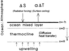
FIGURE 1
Schematic of the geometry of the box-diffusion-upwelling model used in these remarks.
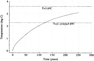
FIGURE 2
Temperature versus time for the impulsive doubling of CO2 at t = 0 in a model with ![]() = 3.6°C.
= 3.6°C.
a = ao/g, where g = system gain, and the relation between g and total feedback, f, is g = 1/(1 − f). Negative f's lead to g < 1, while f > 1 implies an unstable system. If we associate a doubling of CO2 with a ΔS (at the surface as opposed to the ''top of the atmosphere") of 1.8 W m−2, then, in the absence of feedbacks, ΔT = 1.2°C. Models that yield ΔT2×CO2 = 4°C involve a gain of 3.3 (or f = 0.7). An idea of the nature of ocean delay can be seen in Figure 2, where we consider the transient response to an impulsive doubling of CO2 in a system where ΔT = 3.6°C. Clearly, the approach to equilibrium is not simply exponential. However, for simplicity of discussion, we will identify a response with a time scale τ, corresponding to the time it takes ΔT to reach to within (1 − 1/e) of its equilibrium value when the system is impulsively forced. Figure 3 shows how τ varies with g. Over the range of interest, the dependence is almost linear. (As Hansen et al. (1985) note, the relation becomes quadratic as H → ∞.)
A main point of these remarks is that in dealing with these simple models, it is occasionally useful to consider τ rather than g, and ΔT2×CO2 rather than ΔS2×CO2 as variables to focus on. Doing so will suggest constraints on both τ and ΔT2×CO2, which can be determined from considering responses to both volcanos and increasing greenhouse gases. It must be emphasized that it is just as useful to use data to constrain the likely response to doubled CO2 as it is to detect the actual response (which might prove small).
Figure 4 shows T vs. t for the IPCC "business as usual" (BAU) emissions scenario (which leads to a quadrupling of "effective" CO2 by 2100; viz., Houghton et al., 1990). The different curves correspond to various choices of equilibrium ![]() . We see (consistent with IPCC results) that expectations for current warming range from 0.15°C for
. We see (consistent with IPCC results) that expectations for current warming range from 0.15°C for ![]() = 0.24°C to 0.8°C for ΔT2×CO2 = 4.8°C. The observed warming over the past century of 0.45°C ± 0.15°C (viz., Figure 5) corresponds to about
= 0.24°C to 0.8°C for ΔT2×CO2 = 4.8°C. The observed warming over the past century of 0.45°C ± 0.15°C (viz., Figure 5) corresponds to about ![]() = 1.2°C,2 but given the natural variability in T, it is difficult to rule out any of the choices on the basis of the observed global
= 1.2°C,2 but given the natural variability in T, it is difficult to rule out any of the choices on the basis of the observed global
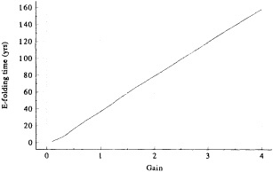
FIGURE 3
Characteristic ocean delay (τ) versus gain (g). See text for discussion.
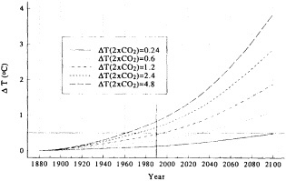
FIGURE 4
Temperature change since 1880 for IPCC "business as usual" emissions scenario and various model sensitivities.
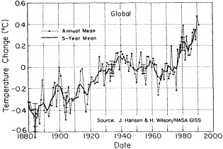
FIGURE 5
Global mean temperature since 1880 (Hansen and Wilson, personal communication).
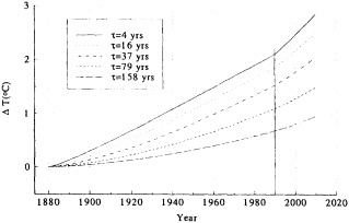
FIGURE 6
Temperature changes since 1880 for IPCC "business as usual" emissions scenario and ΔT2×CO2 = 4°C for various choices of characteristic ocean delay.
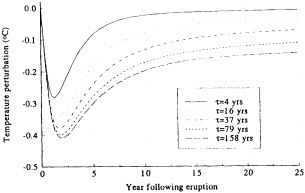
FIGURE 7
Response of global temperature to Krakatoa-type eruption for various choices of characteristic ocean delay.
warming. It is also worth pointing out that none of the choices of ![]() leads to more than 3.5"C of warming by the year 2100—despite the fact that effective CO2 is assumed to have quadrupled, and hence for
leads to more than 3.5"C of warming by the year 2100—despite the fact that effective CO2 is assumed to have quadrupled, and hence for ![]() = 4.8°C the equilibrium warming in 2100 would be 9.6°C. This dramatically illustrates the importance of ocean delay.
= 4.8°C the equilibrium warming in 2100 would be 9.6°C. This dramatically illustrates the importance of ocean delay.
The question we deal with is whether we can do better than the above in constraining expectations. We wish to suggest that the answer may well be yes. Figure 6 shows T vs. t for ![]() = 4°C and various choices of τ (again using the IPCC BAU scenario). Here we see that for
= 4°C and various choices of τ (again using the IPCC BAU scenario). Here we see that for ![]() = 4°C to be compatible with the observed warming, τ must be greater than 100 years. The point is that natural variability is unlikely to cancel out more than about 0.5°C of warming over relatively short periods. There are, indeed, model results that suggest both
= 4°C to be compatible with the observed warming, τ must be greater than 100 years. The point is that natural variability is unlikely to cancel out more than about 0.5°C of warming over relatively short periods. There are, indeed, model results that suggest both ![]() = 4°C and short τ's (Manabe et al., 1991), but as we see here, such suggestions are highly problematic.
= 4°C and short τ's (Manabe et al., 1991), but as we see here, such suggestions are highly problematic.
We finally turn to volcanos. Wigley and Raper (1995) note that atmospheric response to volcanic dust is largely independent of τ because of the short time scales involved. These claims are true only for the first year or two after eruption. For longer times, there are significant dependencies. We represent the forcing from a volcano as ΔS = kt for t ≤ 3 months, and ΔS = S0e−t/d for t > 3 months, where S0 = k × 3 months = 9.3 W m−2, and d = 13 months. These values are crudely chosen to correspond to Krakatoa (Oliver, 1976). Figure 7 shows the response to a single eruption for various choices of τ (or, equivalently, of gain, using Figure 2). We see that we can expect a cooling of 0.25-0.35°C within a year or two of eruption, regardless of climate gain.3 However, for large τ (or system gain) long-term behavior is very different. For short τ's (τ < 16 years or g < 0.5) the cooling maximizes by t = 1 year and decays to relatively undetectable levels within less than 10 years. However, for longer τ's almost half the maximum cooling persists for many years. Also, the maximum cooling seems to occur at t = 2 years rather than 1 year. Neither of these features has been much remarked on. What is going on is that the short-term volcanic cooling is disequilibrating the surface temperature vis-à-vis both the atmosphere and the ocean. For long τ'S, the atmospheric coupling is weak and the ocean delay plays a larger role. Detecting such differences for a single volcano is likely to be non-trivial. Figure 8, from Hansen et al. (1992), shows predicted responses to Pinatubo in a general-circulation model with different assumed greenhouse-warming scenarios. The upper panel clearly shows that Pinatubo leaves
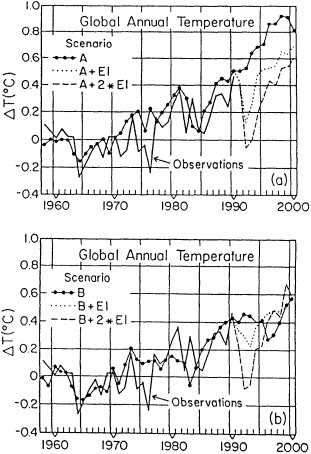
FIGURE 8
Response to Pinatubo for various scenarios calculated by Hansen et al. (1992). See text for details. (From Hansen et al., 1992; reprinted with permission of the American Geophysical Union.)
global temperature cold compared to the expected warming for a long time; however, the lower panel fails to show this persistence in a model where expected greenhouse warming is reduced. A reading of the text of Hansen et al. (1992)
TABLE 1 Ersatz Distribution of Volcanic Eruptions
|
Year of Eruption |
Actual Volcano(s) |
Relative Magnitude |
|
1883 |
Krakatoa |
1.000 |
|
1885 |
Falcon Island |
0.100 |
|
1886 |
Tarawera, Niafu |
0.500 |
|
1888 |
Bandai San, Ritter Island |
0.375 |
|
1892 |
Bogoslav (1890), Awu |
0.150 |
|
1902 |
Una Una (1898), Mt. Pelée, Soufrière |
0.400 |
|
1903 |
Santa Maria, Minami Iwoshima (1904) |
0.630 |
|
1907 |
Shtyubelya Sopka |
0.150 |
|
1912 |
Taal (1911), Katmai, Sakurashima (1914) |
0.185 |
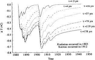
FIGURE 9
Calculated response to all volcanos between Krakatoa and Katmai for various choices of model gain (expressed in terms of characteristic ocean delay).
shows that this scenario also included an additional volcanic eruption in 1995!
There would appear to be some possibility of distinguishing different t's by considering sequences of volcanos, since larger t's imply cumulative effects for a sequence of volcanos while smaller t's imply largely independent responses to each individual volcano within a sequence.
These considerations should be relevant to the period 1883-1912 (Krakatoa to Katmai), when there were a number of major eruptions whose total dust production was about three times that of Krakatoa alone (Oliver, 1976). This period was followed by a relative absence of eruptions until about 1950. We have modeled the volcanism of the period 1883-1912 by an ersatz distribution in which various closely spaced eruptions are combined. This is described in Table 1. Figure 9 shows the response to this distribution of volcanism for various choices of t. Clearly, for larger t's (greater than 16 years) each eruption adds cooling to the response of successive volcanos, leading to cumulative, long-lasting cooling following the period 1883-1912, while for smaller t's (less than 16 years) the response has little cumulative character, although the large number of eruptions leaves the temperature depressed for the period 1883-1912.
On the whole, the temperature record shows no evidence of a cumulative effect of volcanism (viz., Figure 5),4 suggesting that appropriate t's are less than 16 years, while Figure
6 suggests that t < 100 years is incompatible with ![]() = 4°C.5 Indeed, reference to Figure 3 suggests that t < 16 years corresponds roughly to g 0.5 and
= 4°C.5 Indeed, reference to Figure 3 suggests that t < 16 years corresponds roughly to g 0.5 and ![]() < 0.6°C.
< 0.6°C.
Certainly, these matters require more careful analysis. However, the present remarks suggest that consideration of a variety of known climate-forcing perturbations as probes of the climate system may allow the use of a simple methodology for constraining our expectations for greenhouse warming. For example, if responses to volcanos imply short characteristic ocean delays, then we would also expect small climate responses to increasing CO2. One will of course want to understand in detail the physics determining climate sensitivity. However, this hardly justifies ignoring the possibility that it may be possible to bypass these details in approaching the issue of sensitivity directly.
ACKNOWLEDGMENTS
I should like to acknowledge the support of the National Science Foundation under Grant 8520354-ATM and of the National Aeronautics and Space Administration under Grant NAGW-525.
|
5 |
Conceivably, support for this conclusion might also emerge if the climate response to volcanos tends to peak at one year rather than two years after eruption (viz., Figure 7). |
Modeling the Possible Causes of Decadal-to-Millennial-Scale Variability1
DAVID H. RIND2 AND JONATHAN T. OVERPECK3
ABSTRACT
There are at least five possible causes of decade-to-century-scale climate variability: inherent ("random") variability in the atmosphere (i.e., no external forcing); inherent or forced variability in the atmosphere-ocean system (e.g., North Atlantic Deep Water fluctuations); solar variability (e.g., the Maunder Minimum); variability in volcanic aerosol loading of the atmosphere (e.g., Tambora); and atmospheric-trace-gas variability (e.g., CO2, methane). Modeling experiments conducted for each of these potential mechanisms show that they have somewhat different signatures, which may allow for discrimination between them in the climate record. The necessary magnitudes of forcing required from the different mechanisms to produce the past climate variations also allow us to estimate the likelihood of their affecting future global change. We conclude that none of them can be dismissed, and we should be prepared for the possibility that several have acted in concert to produce the variability seen in the climate record.
INTRODUCTION
The paleoclimate record contains many examples of apparently significant decade-to-century-scale climate variability, including variations in both temperature and moisture balance (Overpeck, 1991; Bradley and Jones, 1992a). The last millennium appears to have featured at least two widespread cool periods lasting a century or more, beginning approximately A.D. 1275 and A.D. 1510, respectively (Bradley, 1990). Shorter cool periods arose in the decades of the 1590s to 1610s, 1690s to 1710s, 1800 to 1810s and 1880s to 1900s, while prolonged warm periods occurred in the 1650s, 1730s, 1820s, 1930s to 1940s, and 1980s (Bradley, 1990). The global synchronicity of these temperature trends, and their geographic distribution, are in many cases not clear, especially for the earlier time periods. Nor are the causative factors understood in most cases. This state of affairs clearly hinders our ability to predict the anthropogenic climate signature, since its magnitude is likely to be similar to that of these past perturbations, at least for the next few decades.
There are at least five potential explanations for global-scale decadal to millennial climate variations. Natural, unforced variability, associated with either atmospheric dynamics or interactions within the climate system (without including ocean circulation changes), is one candidate; this potential explanation obviates the need to search for "causative" factors of the observed climate changes, and simply relies on the mechanisms inherent to the system. Extending this concept to include ocean circulation changes broadens the range of possibilities. Fluctuations in the atmosphere-ocean system are observed to occur today and might be a natural characteristic over longer time scales, although they could equally well come into existence as a response to changes in climate forcing. Solar variability exists as a favorite "wild card" possibility, legitimized to some extent by recent observations of solar irradiance changes during the most recent solar cycle. Volcanic aerosol injections appear to cool the climate, and a clustering of such events, or the lack of such events, would likely lead to a change in mean climate. Finally, variations in greenhouse trace-gases such as CO2 and methane have been observed to occur over the last several hundred years, with cumulative climate impact.
Given the lack of quantitative measurements of some of these forcings over time, one approach to estimating the cause(s) of decade-to-century-scale variability is to model each of these perturbations in a generic sense and compare the results to climate reconstructions. The model used for experiments done specifically for this paper is the GISS general circulation model (GCM) (Hansen et al., 1983b), run at 8° × 10° resolution, with sea surface temperatures either prescribed or calculated, as indicated in Table 1. This model has a sensitivity of 4.2°C warming for 2 × CO2 (or an increase of 2 percent in the solar constant) (Hansen et al., 1984), with a high-latitude/low-latitude sensitivity of about a factor of 2. The quantitative calculations given below are a function of this model sensitivity. Calculations from other GCMs are noted where appropriate.
The model results indicate that each of the potential explanations of climate variability listed above has its own characteristic signature that may provide a basis for discrimination in the climate record. In the subsequent sections we will discuss evidence suggestive of the various forcings, as well as relevant modeling studies depicting the possible nature of the climatic response. We concentrate mostly on temperature, since it is this parameter that is most often recoverable in the paleoclimatic data on these time scales. In the discussion section, we will briefly review what evidence is needed to decide on which causes are most likely.
NATURAL VARIABILITY
Natural variability suggests an unforced oscillation in climate parameters. It can arise primarily from atmospheric dynamics or from atmospheric thermodynamics. In either mode it must alter the net heating of the surface, either locally, if that is all that is involved, or globally. For oscillations of multidecadal scale to be set in motion, portions of the system with large heat capacities or time constants (ocean, cryosphere) must be involved, or interactions setting in motion positive feedbacks (water vapor, cloud cover), which ultimately reverse direction, must arise. The ocean mixed layer by itself has an e-folding time constant of a few years, with an impact that can be lengthened via other feedback processes (Hansen et al., 1985). An example of the "reversing-direction" process, somewhat analogous to the mechanism proposed by Ramanathan and Collins (1991) although operating on a longer time scale, could be as follows: Warmer sea surface temperatures lead to an increase in high-level clouds and thus to a further greenhouse amplification of sea surface temperatures; eventually the clouds become sufficiently optically thick to reduce incoming solar energy, which set in motion a cooling of the surface and additional water-vapor feedbacks. Wigley and Raper (1990) suggested that high-frequency climate forcing, perhaps associated with clouds, could extend to a century-scale oscillation of a few tenths of a degree Celsius via the ocean's thermal inertia.
TABLE 1 GCM Experiments Discussed in the Text
|
Experiment |
Duration |
Ocean Temperatures |
|
Unforced variability |
100 years |
Calculated SSTs, with mixed-layer depth (MLD) averaging 125 m |
|
Reduced North Atlantic SSTs |
6 years |
Prescribed colder North Atlantic SSTs, 1/5 full ice-age cooling |
|
Reduced solar inputs of -0.25% or -2% |
55 years each |
Calculated SSTs with MLD of 65 m |
|
Added volcanic aerosols t = 0.15 |
55 years |
Calculated SSTs with MLD of 65 m |
We begin with the possibility of dynamically induced climate changes. Inherent variability in the atmosphere, possibly associated with non-linear dynamics, is thought to be capable of generating intraseasonal variability. Hansen and Sutera (1986) utilized a planetary-wave activity index to resolve two modes of Northern Hemisphere winter 500 mb height distributions, one with low and one with high amplitudes. The differences between the height fields are centered over the Aleutians, north central Canada, and western Europe. If these two modes represent interannual tendencies that might be selectively activated, they could conceivably set in motion climate feedbacks (snow, sea ice, ocean mixed-layer depth) with climate implications and longer time scales. It is not known whether the modes are forced or simply the result of non-linear dynamics. This type of "natural" variability must be considered speculative when applied to the climate domain. Additional decadal variability may be found in meridional modes of the coupled ocean-atmosphere system that propagate from pole to pole over 3- to 20-year time periods (see, e.g., Mehta, 1992). Their relationship to climate variability is also unproven.
Hansen et al. (1988) ran a GCM with a mixed-layer ocean for 100 years (Table 1). The model produced an oscillation of 0.5°C (peak to peak) over that interval without any external forcing (Figure 1, top). As emphasized by Barnett et al. (1992), an inversion and slight time shift of
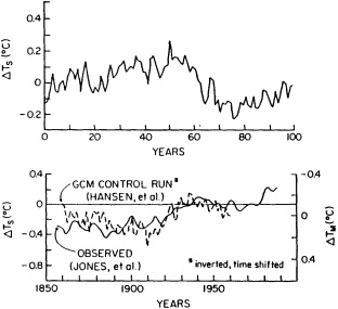
FIGURE 1
Top: Global-mean (unforced) surface air temperature variations in a 100-year control run with an atmospheric GCM and mixed-layer ocean model. (From Hansen et al., 1988; reprinted with permission of the American Geophysical Union.) Bottom: An inversion and time shift of the results shown in the top figure, compared with observed temperature changes over the past 100 + years. (From Barnett et al., 1992; reprinted with permission of the American Geophysical Union.)
this record results in matches to a number of the features in the observed temperature record from 1850 to 1950 (Figure 1, bottom). The implication is that the system is capable of producing such temperature oscillations without the need for causative factors (i.e., forcing).
As analyzed by Barnett et al. (1992), the primary contributions to the temperature oscillation occurred in the tropics (Figure 2); over 90 percent of the variability was located within 30° latitude of the equator. The oscillation was largely the result of a cloud cover/sea surface temperature correlation: Low clouds increase as the ocean cools, further reducing the net heating of the surface. At least part of this correlation was due to the sub-grid-scale temperature parameterization used in the GCM. In contrast to these results, the observed variability over the last century has been dominated by high-latitude contributions (Hansen et al., 1983a). Thus there is good reason to doubt that the variability found in the GISS GCM 100-year run is a convincing indicator of the natural variability in the climate system. The inclusion of additional processes, such as ocean dynamics, variations in cloud optical thickness, and the heat exchange with the ocean below the mixed layer would improve the model's realism (Barnett et al., 1992).
Manabe et al. (1991) produced similar-looking temperature global variations in a 100-year simulation with a fully coupled atmosphere-ocean GCM. The greatest persistence was found in the polar oceans of both hemispheres, due to their weaker thermal damping (reduced surface and radiative heat fluxes) and deep mixing. The relevance of this run to real-world oscillations is limited by the continuously specified input of heat and salinity to the ocean; while this input does not vary from year to year, its very existence will perturb the model's own natural variability, and the necessity for incorporation of these fluxes raises doubts about the model's accuracy.
In yet another unforced 100-year simulation with a coarse-resolution model and a mixed-layer ocean, Houghton et al. (1991) found decadal and longer-time-scale variability in sea surface temperatures; in fact, the sea surface temperature at low and middle latitudes had a distinctly red spectrum. The percentage of variance in the low-frequency range (4 to 100 years) showed a small increase with latitude, with high-latitude effects associated with decadal-scale sea-ice variability (as has been noted by Mysak et al. (1990) in the Greenland and Labrador seas). The simulated global surface air temperature did not display significant multidecadal-scale variability, mainly because little such variability arose in the tropical middle-latitude domain (in contrast to the GISS model results). Cloudiness was not allowed to change in these experiments, which it could in the GISS model.
In summary, the unforced decade-to-century-scale oscillations of global temperature that characterize the natural climate system may well be on the order of several tenths
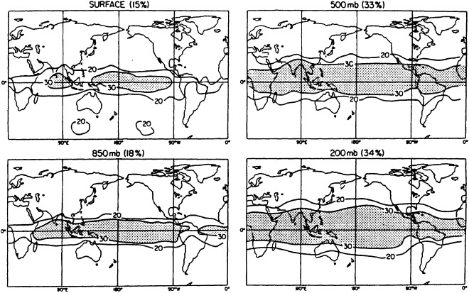
FIGURE 2
Geographical distribution of the first empirical orthogonal function (EOF) of the surface air temperature changes from Figure 1. The percentage of variance represented by this EOF is given for the different levels. (From Barnett et al., 1992; reprinted with permission of the American Geophysical Union.)
of a degree Celsius, although this has not been proven satisfactorily. At the very least, the model results imply that oscillations of this magnitude may be expected to occur without changes in external forcing.
VARIABILITY OF THE OCEAN-ATMOSPHERE SYSTEM
The El Niño/Southern Oscillation (ENSO) phenomenon represents a well-studied example of atmosphere-ocean oscillations. The ability of this type of localized forcing to alter global patterns of temperature and precipitation indicates that it could have an effect on globally averaged climate (Ropelewski and Halpert, 1987), and the El Niño occurrence itself is generally associated with a global mean temperature change of about 0.1 to 0.2°C. The prevalence of El Niños during the past several decades and the lack of pronounced La Niñas undoubtedly have influenced global temperatures (Trenberth, 1990). A key question is whether the frequency of El Niño occurrences fluctuates with time. The results of analysis are equivocal; for example, there are some indications that fewer events took place during the period from the 1920s to the 1950s (Cooper et al., 1989), while others claim that 1925 to 1932 was a period of unusual activity (Quinn et al., 1987). Cole (1992) has investigated the variance of ENSO activity as reflected in coral records for the past century and found that the dominant frequencies have changed significantly. This observation serves to emphasize that ocean-atmosphere oscillations may themselves be the result of external forcing, a subject we will return to below.
Changes in the ocean heat transport, associated with changes in the wind-driven circulation or the large-scale thermohaline circulation, represent an obvious method of inducing climate variability (see, e.g., Weyl, 1968; Watts, 1985; Rind and Chandler, 1991). The "Great Salinity Anomaly" in the North Atlantic was apparently associated with colder temperatures during the late 1960s and 1970s and reduced deep-water formation (Brewer et al., 1983; Lazier, 1980). The Younger Dryas cooling event (from ca. 11,000 to 10,000 years B.P.) is a much-cited example of North Atlantic Deep Water (NADW) reduction that led to cooling, at least in the region of the North Atlantic (e.g., Broecker et al., 1985). The same type of process may have played
a role in the Little Ice Age, judging from the pattern of cold, dry winters over Europe (Pfister, 1992). As in the case of altered El Niños, variations in deep-water production could be a natural characteristic of the system, or they might be forced by other mechanisms; the Younger Dryas event may have been initiated by melting of land ice associated with the general deglaciation (Broecker et al., 1988), while the Great Salinity Anomaly could have been a random perturbation on decadal time scales.
How cold was the Little Ice Age, and how much would ocean heat transports have had to be reduced to produce the observed cooling? Mountain glaciers advanced by some 100 to 200 m (Porter, 1975; Broecker and Denton, 1989), equivalent to about one-fifth of their reduction since the full ice age (Rind and Peteet, 1985). If the cooling was also one-fifth as large, we can reduce the North Atlantic sea surface temperatures by one-fifth their full glacial reduction and use a GCM to estimate the resulting regional and global changes in atmospheric temperature. The temperature perturbation associated with this North Atlantic cooling (Table 1), which is reminiscent of a reduction in NADW formation, is shown in Figure 3. Cooling is basically constrained to downstream locations in Eurasia, and immediately upstream in the vicinity of the eastern United States. Note that if sea surface temperatures in other parts of the ocean had been involved (e.g., the North Pacific) the cooling would have been more widespread. Other aspects of the model simulation also appear realistic: Associated with the colder sea surface temperatures there is higher pressure and lower precipitation over Europe, in good agreement with reconstructions for the Little Ice Age (Pfister, 1992).
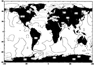
FIGURE 3
Annual average surface-temperature change in the GISS GCM due to colder North Atlantic sea surface temperatures. Temperatures were reduced by one-sixth of the full glacial cooling for the North Atlantic, in accordance with the relative reductions in alpine glaciers for the two time periods, from 30°N to the pole, consistent with the location of observed sea surface temperature changes in the Younger Dryas (Rind et al., 1986). (From Rind and Overpeck, 1994; reprinted with permission of Pergamon Press.)
The ocean heat-transport reduction necessary to produce this cooling is given in Figure 4. Peak reductions are 25 percent in the North Atlantic, concurrent with increased poleward heat transport in the South Atlantic. For the North Atlantic as a whole, poleward heat transports are reduced by 20 percent; this can be contrasted with estimates of North Atlantic transport reduction during the full ice age of some 70 percent (Miller and Russell, 1989). If the heat transport changes are at all proportional to changes in NADW production, it would imply a Little Ice Age change in NADW production two-sevenths the magnitude of the full ice age reduction, a fraction somewhat similar to that of the advance of the ice lines in the Little Ice Age compared with the advance in the full ice age.
SOLAR VARIABILITY
The hypothesis of solar forcing of weather and climate is at least a century old (Blanford, 1891). The relationships between sunspots and various weather phenomena have been described in numerous publications, some implying statistical significance. The percentage of variance explained increased dramatically when sunspot-cycle effects were partitioned according to the phase of the equatorial zonal wind, the quasi-biennial oscillation (QBO) (van Loon and Labitzke, 1988). While the reality of this effect is still being debated (e.g., Barnston and Livezey, 1989; Baldwin and Dunkerton, 1989), its existence could have climatic implications to the extent that it would heighten the sensitivity of the troposphere to perturbations (i.e., ultraviolet radiation fluctuations) that directly affect the stratosphere.
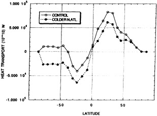
FIGURE 4
Implied Atlantic Ocean poleward heat transports, between longitudes 70°W and 10°E for the current climate control run, and the experiment with reduced North Atlantic sea surface temperatures. Ocean heat transports are calculated from the net energy forcing at the ocean surface, as described in Miller and Russell (1989). (From Rind and Overpeck, 1994; reprinted with permission of Pergamon Press.)
Investigations of solar forcing of climate variability have focused on longer-term periodicities associated with the near-absence of sunspot cycles (e.g., Stuiver et al., 1991). Sunspot records have been deduced from observations, although they are quite uncertain prior to 1800, and from variations in carbon and beryllium isotopes. In periods of high solar activity, the stronger solar wind deflects cosmic rays and decreases the production of cosmogenic isotopes, so solar activity is typically thought to be responsible for much of the natural decade-to-century-scale changes in 14C and 10Be (Stuiver et al., 1991; Stuiver and Braziunas, 1988). Long-term 14C variations can be determined by comparing 14C dates with dates obtained from analyses of tree rings, whereas records of 10Be variations are obtained from ice cores. Although care needs to be taken in interpreting 14 C changes, since they are affected by the intensity of the geomagnetic-field polar dipole and carbon-cycle/climate variations, the covariation between 14C and 10Be suggests strong solar control of isotope production for the time scales of concern here (Stuiver et al., 1991).
Spectral analyses of the 14C record indicate apparent fluctuations in periods ranging from decades up to several thousand years, including the 11- and 22-year (Hale) cycles, the 88-year (Gleisberg) cycle, and approximately 200-year and approximately 2500-year cycles (see, e.g., Damon and Linick, 1986; Stuiver et al., 1991). Hints of these cycles have also been identified in the climate record, e.g., the 2500-year cycle in marine, glacier, and polar ice core records (Pestiaux et al., 1987; Denton and Karlen, 1973; Wigley and Kelly, 1990; Dansgaard et al., 1984), and the 88- and 200-year cycles in varved sediments (Halfman and Johnson, 1988; Peterson et al., 1991; Anderson, 1992). Whether these are truly periodic in nature is doubtful, and the relationship of the geologic indicators to climate is itself uncertain, but the similarities in periodicities are indicative of a general coincidence of apparently reduced 14C production and colder temperatures (de Vries, 1958; Eddy, 1976), with the Maunder Minimum/Little Ice Age being the most recent example.
To quantify this connection, it is necessary to know the magnitude of the possible solar irradiance variations. Recent observations during the last solar cycle (solar cycle 21) indicated close to 0.1 percent peak-to-peak change from solar maximum to solar minimum (e.g., Willson and Hudson, 1991). What these observations imply about past solar irradiance variations is a more difficult question. Various indicators of insolation changes have been generated. These include 10Be and 14C variations, indicative of solar activity (Beer et al., 1988, 1990; Stuiver et al., 1991); solar-radius variations, thought to be representative of solar luminosity (Ribes et al., 1987); the envelope of the sunspot cycle, perhaps representative of solar irradiance and apparently correlated with decade-to-century-scale sea surface temperature variations (Reid, 1991); and the length of the solar cycle, also seemingly correlated (Friis-Christensen and Lassen, 1991). These latter correlations have been used to suggest the possibility of solar dominance of climate variability over the last several centuries. In recent publications, Kelly and Wigley (1992) and Schlesinger and Ramankutty (1992) both found that including solar irradiance variations related to the length of the solar cycle improved their reconstruction of global temperature changes for the last 150 years. Nevertheless, it is difficult to translate these solar properties into absolute irradiance changes and prove the causal connection.
Another approach to understanding solar variations has been to observe other stars that have a nature similar to the sun's. Decadal-scale stellar-activity variations are apparent (Radick et al., 1990), including the complete absence of "sunspot" conditions (Baliunas and Jastrow, 1990). Accompanying variations in luminosity are as much as 0.4 percent, or somewhat higher than the variation recorded in solar cycle 21. While the relevance of these observations to solar irradiance variations is uncertain, they do serve to provide some constraint on the magnitude of likely changes.
Lean et al. (1992) estimate that the Maunder Minimum reduction in solar insolation was on the order of 0.25 percent, due to changes in sunspots, faculae, and network radiation. Current GCMs give a climate sensitivity of approximately 4°C for a 2 percent change in solar constant (Hansen et al., 1984); whether the 0.25 percent reduction is sufficient depends on how cool the Little Ice Age was. Estimates range from 0.5°C (Wigley and Kelly, 1990) to 1°C to 1.5°C (Crowley and North, 1991). The nominal value we have used above, about one-fifth the cooling of the full glacial age, implies values of 0.7°C to 1.0°C (e.g., see Rind and Peteet (1985) for estimates of the full ice-age cooling of 3.5°C to 5°C). A GCM simulation with the GISS model, using the 0.25 percent reduction, produced a global annual-average cooling of about 0.45°C, which is probably somewhat smaller than would be required to explain the Little Ice Age if solar variability were acting alone. Of course, if the climate sensitivity were greater or the global temperature change smaller than indicated, the required solar variability would be reduced.
The geographical variation of the temperature change generated by the 0.25 percent reduction (Table 1) is shown in Figure 5. Significant cooling occurs in the tropics, and there is no obvious high-latitude amplification of the climate change. Note that not all regions are cooler than they are today; the forcing is small enough that regional changes in advection patterns can produce local warming. A similar response occurred in the colder-North-Atlantic experiment, which produced advective warming over the Arctic (Figure 3). These results imply too that advection changes may also alter the sources of water vapor sufficiently to confound isotope/temperature reconstructions when the cooling is of such small magnitude (Cole et al., 1992).
The low-latitude cooling led to a reduction in the intensity
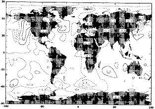
FIGURE 5
Annual average surface air temperature changes resulting from a flat spectrum decrease in the solar irradiance of 0.25 percent in the GISS GCM. Results are for years 46 to 55 of the simulation. (From Rind and Overpeck, 1994; reprinted with permission of Pergamon Press.)
of the tropical portion of the Hadley circulation by 5 to 10 percent. Because reductions in Hadley-cell intensity are a possible cause of ENSO events, this result is qualitatively consistent with the Enfield and Cid (1991) correlations of strong El Niños and low solar activity. As will be discussed below, volcanic aerosol could also play this role, perhaps more efficiently.
An additional problem is the wavelength distribution of the radiation fluctuations. During the last solar cycle, 20 percent of the observed solar irradiance variations have been in the ultraviolet range, having wavelengths short of 300 nm, with magnitudes as presented in Figure 6 (Lean, 1987; Cebula et al., 1992). This radiation is all absorbed in the middle and upper atmosphere, above the tropopause. In a
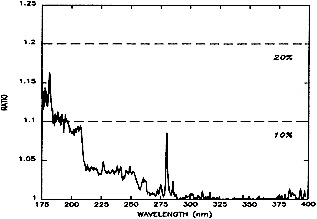
FIGURE 6
Solar ultraviolet irradiance variability as observed in solar cycle 21 (Lean, 1992, personal communication). (From Rind and Overpeck, 1994; reprinted with permission of Pergamon Press.)
GCM experiment with an increase in total solar radiation of 0.5 percent, but with all wavelengths restricted to less than 300 nm, we found that there was no increase in solar heating at levels below the tropopause. Thus, the ability of solar irradiance variations to replicate observed climate variability will depend on the frequency of the radiation affected, in addition to its magnitude. A change in UV radiation absorbed in the stratosphere might conceivably be able to influence climate if the impact on tropospheric dynamics described by van Loon and Labitzke (1988) proves to be real.
VOLCANIC AEROSOLS
Previous studies (Lamb, 1970; Bray, 1974; Porter, 1981; Grove, 1988) have suggested that the trends in global climate observed during the years A.D. 1000 to 1800 could largely be explained by variations in volcanic aerosol forcing. Porter (1986) related acidity records in the Greenland ice cores to alpine glacial fluctuations in the Northern Hemisphere and found a reasonably good correlation, with increased acidity during periods of glacial advance. It is recognized that high-latitude ice cores may overemphasize mid- and high-latitude volcanic eruptions (Bradley and Jones, 1992b), which should be less effective in altering global climate than low-latitude eruptions. Furthermore, cold periods with low precipitation may have higher acidity concentrations because there has been less dilution from snowfall. Nevertheless, as the recent estimates of a 0.5°C cooling associated with Mt. Pinatubo (Hansen et al., 1992) suggest, volcanic aerosols (primarily sulfuric acid) have the capability to significantly alter the global climate (Rampino and Self, 1984).
What magnitude and frequency of volcanic eruptions are required to produce the cooling estimated for the Little Ice Age? We can use several recent GCM experiments with Mt. Pinatubo (Hansen et al., 1992; Rind et al., 1992; Pollack et al., 1993) to provide estimates. Aerosol radiative forcing depends on geographical distribution, optical depth, size distribution, composition, and altitude; however, as shown by Lacis et al. (1992), the forcing of tropospheric climate is primarily a function of aerosol-column optical depth, assuming a global distribution. In a study of transient volcanic aerosol, a volcanic eruption with a peak global optical thickness of 0.18 (on the order of what has been observed for Mt. Pinatubo) and an e-folding time of 12 months (so that in 3.5 years 97 percent of the aerosols will have been removed) produced a peak cooling of 0.5°C in year 2, and a three-year average cooling of 0.3°C (Hansen et al., 1992). In another experiment, with one-half the optical thickness and the same residence time, the cooling was reduced by a factor of 2. If this linearity holds for increased optical thickness values as well, it implies that to produce a global cooling of some 0.5°C to 1.0°C on a three-year average, via a transient volcanic eruption, would require a volcanic-
aerosol injection of 2 to 3 times the magnitude of Mt. Pinatubo's. The Tambora eruption of 1815 may have been of this magnitude (Rampino and Self, 1982).
However, if volcanic aerosols were maintained continuously in the atmosphere, i.e., their climate forcing remained relatively constant, then the ocean would have sufficient time to respond to them and to initiate positive feedbacks amplifying the cooling. With an optical thickness of 0.15 (equivalent to a 2 percent decrease in solar constant), the GISS model produces an equilibrium cooling of some 4.7°C after 50 years (Rind et al., 1992; Pollack et al., 1993). To produce a 0.5°C to 1°C cooling would take an optical thickness approximately one-sixth as large, or 0.025. This is some five times larger than the ''non-volcanic" background that existed during much of the time from 1900 to 1960, and it could be achieved by the eruption of a Mt. Pinatubo once every eight years, or, equivalently, of an El Chichon every fifth year. Over the last 100 years, we have had two events of the latter magnitude (Mt. Agung and El Chichon), and one of approximately twice this magnitude (Mt. Pinatubo). Thus, volcanic-aerosol-induced cooling of the appropriate magnitude would require a substantial increase in large volcanic injections. (Also, to be effective globally, they would have to originate in low latitudes, although a big high-latitude eruption might have a significant regional or hemispheric impact.)
Is there any way to distinguish global volcanic-aerosol cooling from reduced solar insolation? We have run two experiments with the GISS GCM and GCMAM (the version of the model that extends up to 85 km altitude). In one, the solar constant was reduced by 2 percent; in the other, the volcanic-aerosol optical depth was increased to 0.15, which is equivalent to a 2 percent reduction in solar energy reaching the surface (Table 1). The relevant differences between the results from the two experiments are given in Table 2. A primary difference is that the reduction in solar irradiance cools the lower stratosphere, while volcanic aerosols induce warming in that region, via short-wave and long-wave absorption (Rind et al., 1992). In conjunction with the slightly greater sea surface cooling in the tropics from the aerosol experiment, volcanoes appear to increase the static stability at low and subtropical latitudes more than does a simple solar energy reduction. With increased stability, the Hadley cell is weakened more in the volcano experiment, and the precipitation gradient between the tropics and Northern Hemisphere subtropics is somewhat reduced. (For example, if a record of precipitation for the Little Ice Age were available at these latitudes, such a change in gradient (about 20 percent) might be observable.) Wetter subtropical deserts might occur more easily with volcanic-aerosol forcing than with a solar irradiance reduction; however, both types of forcing appear to weaken the Hadley circulation somewhat.
In this section we have been concerned with the influence of volcanic aerosols, but tropospheric aerosols may well have increased over the past few centuries, thus cooling the climate (Charlson et al., 1992). The increase in aerosol-cooling effect through time does not allow for any obvious influence on earlier cold oscillations, but if the magnitude of the reduction in solar irradiance is as large as hypothesized in the IPCC (1992) report, aerosols would counter much of the effect of trace-gas variations, discussed below. There is still much uncertainty concerning historical variations in the direct global effect of tropospheric aerosol scattering, and even more uncertainty in aerosols' influence on cloud cover.
TRACE-GAS VARIATIONS
Ice-core evidence of trace-gas concentrations during the last several centuries has indicated that CO2 levels were at approximately 270 ppm for some time prior to this century (Neftel et al., 1985) (they are currently close to 360 ppm), and that methane has increased from around 0.8 ppmv to its current value of 1.72 ppmv (Rasmussen and Khalil, 1984). Such variations in greenhouse gases undoubtedly have had an effect on the climate system. They complicate the issue of the Little Ice Age cooling because they can add a linear trend to whatever fluctuations might have occurred—that is, the cooling that would be required to reduce current temperatures to Little Ice Age values is increased due to the trace-gas-induced warming over the last several hundred years.
To estimate the influence that these trace-gas variations may have had, two facts need to be known: The equilibrium response of the system, and the response that has occurred so far. The equilibrium response can be calculated with the formulae presented in Hansen et al. (1988). For CO2, the global-average radiative surface-temperature change due to a change in gaseous concentration X (in ppm) can be calculated as
where
A CO2 reduction from 315 to 270 ppm thus gives a ΔT (radiative) of 0.30°C.
The equilibrium feedback factor to radiative perturbations in GCMs is between 3 and 4 (Hansen et al., 1984). Therefore, in equilibrium the CO2 change would provide for a cooling of about 1°C.
For methane, the equilibrium temperature change to a change in methane (in ppmv) can be calculated as
TABLE 2 Differences Between Experiment with Volcanic Aerosal Optical Depth Increased to 0.15 and Experiment with Solar Irradiance Reduced by 2 Percent
|
Latitude (degrees) |
T (68 mb) |
Surf Temp., Global (°C) |
Surf Temp., Land (°C) |
Precip., Global (mm/day) |
Precip., Land (mm/day) |
|
90 |
-1 |
0.8 |
0 |
-0.1 |
0 |
|
82 |
-1 |
0.3 |
-0.7 |
-0.1 |
-0.1 |
|
74 |
- |
0 |
-0.5 |
0 |
-0.1 |
|
67 |
0 |
0 |
0 |
0 |
0 |
|
59 |
0 |
0.1 |
-0.3 |
0 |
0 |
|
51 |
1 |
-0.4 |
-0.6 |
0 |
-0.1 |
|
43 |
1 |
-0.1 |
-0.6 |
0 |
0 |
|
35 |
2 |
-0.3 |
-0.8 |
0 |
0 |
|
27 |
2 |
-0.5 |
-0.6 |
0 |
0 |
|
20 |
2 |
-0.6 |
-0.7 |
0 |
-0.1 |
|
12 |
3 |
-0.6 |
-0.7 |
0 |
-0.1 |
|
4 |
3 |
-0.7 |
-0.9 |
-0.1 |
-0.4 |
|
-4 |
3 |
-0.7 |
-0.9 |
-0.3 |
-0.4 |
|
-12 |
3 |
-0.8 |
-0.6 |
-0.3 |
-0.1 |
|
-20 |
2 |
-0.8 |
-0.2 |
0 |
-0.2 |
|
-27 |
1 |
-0.4 |
-0.5 |
-0.2 |
-0.1 |
|
-35 |
1 |
-0.4 |
0.1 |
0 |
0 |
|
-43 |
1 |
-0.4 |
0.7 |
-0.1 |
0 |
|
-51 |
1 |
0.8 |
0.2 |
0 |
0.2 |
|
-59 |
0 |
1 |
-0.2 |
0 |
0.1 |
|
-67 |
0 |
0.3 |
0 |
0 |
0 |
|
-74 |
0 |
-0.1 |
0.3 |
0 |
-0.1 |
|
-82 |
-1 |
0 |
0 |
0 |
0 |
|
-90 |
-1 |
0.3 |
0 |
0 |
0 |
|
GLOBAL |
1.4 |
-0.34 |
-0.45 |
-0.04 |
-0.08 |
where
A methane reduction from 1.5 ppmv to 0.7 ppmv corresponds to a radiative temperature change of 0.08°C. With the estimated feedback, this gives an equilibrium temperature change of close to 0.3°C.
The observed variation in CO2 and methane in an equilibrium calculation would thus correspond to a temperature change over the last several hundred years of about 1.3°C, with the currently estimated feedback factors. This alone would be sufficient to account for much of the Little Ice Age cooling, without the additional forcing generated by recently added trace-gases (e.g., CFCs). (However, this correspondence also ignores the potential impact of increases in tropospheric aerosols, which, as noted above, may have acted to force the system in the opposite direction, with a magnitude similar to that of the trace-gas effect.) It therefore raises the question of what fraction of this equilibrium response has been observed, i.e., what the response time of the system is. Hansen et al. (1985) discuss the various estimates for this value, noting that it is a function of both ocean mixing (which determines the effective heat capacity of the system) and climate sensitivity (which is indicative of the magnitude of the feedbacks that must come gradually into play; note that if there are no feedbacks, then all the forcing arises instantaneously from the initial perturbation, reducing the delay in system response).
With an effective vertical diffusion through the base of the mixed layer on the order of 1.5 cm2 s-1, as implied by transient ocean tracers (Broecker et al., 1980), and a feedback factor of the magnitude noted above, the CO2-induced warming from 1850 to 1980 amounts to approximately one-third of the equilibrium response (Hansen et al., 1985). For an approximately similar phasing of methane changes, as indicated by the above references, the proportion of equilibrium warming should be similar. Thus we might conclude that only one-third of the equilibrium trace-gas response has been realized, or approximately 0.4°C to 0.5°C. Nevertheless, if the Little Ice Age was 1°C cooler than today, half of this could be a trace-gas effect, with most of the related warming occurring in the twentieth century. Since the trace-gases are globally distributed, the climate changes
they induce would be similar to those shown for solar radiation reduction (Figure 5), since doubled CO2 and a 2 percent solar constant increase yield similar patterns of model response (Hansen et al., 1984).
DISCUSSION
The different forcings and natural variability discussed above have in many cases different geographical expressions (see, e.g., Figures 2, 3, and 5, and Table 1). For example, the forcing that is of radiative importance globally, such as reduced insolation or continual volcanic-aerosol injections, has a larger impact at inland locations away from the moderating influence of the ocean. In contrast, changes in ocean heat transport and NADW production have maximum influence in coastal locations. The former type of forcing would therefore imply maximum Little Ice Age cooling in central Eurasia, decreasing toward the Atlantic coast, whereas the opposite would prevail if NADW-formation changes were acting alone.
It might therefore appear to be possible to distinguish between them through reference to paleoclimatic data for the last several centuries. A joint NSF/NOAA project, Analysis of Rapid and Recent Climate Change (ARRCC), has begun reconstructing the geographical climate distribution for several time periods during the last few hundred years, with this goal in mind. Worldwide distributions of temperature and precipitation changes will be needed for this purpose. Whether the data are sufficiently comprehensive and accurate remains to be seen.
A complementary approach involves reconstructing the potential climate forcing for this time period, whether it be solar irradiance, volcanic aerosols, trace-gases, or ocean circulation. As noted above, there are many empirical estimates of solar irradiance variations, but they need to be quantified on the basis of physical principles. The actual volcanic-aerosol properties are similarly difficult to constrain (Bradley and Jones, 1992b). It may be possible to deduce ocean-circulation changes through biological/ geochemical studies in high-resolution sediment and coral cores, but that is not yet certain.
With both the climate response and climate forcing somewhat ambiguous for these time periods, in this paper we have had to rely on current climate models to suggest possible links. The major problem here is that we cannot be sure that the models have the proper climate sensitivity, either globally or locally. Analysis of climate forcing on the time scale of glacial/interglacial epochs suggests that we probably know the global sensitivity to within a factor of 2 (Lorius et al., 1990). The shorter-term response is hard to calibrate, and its latitudinal expression is likewise somewhat uncertain, beyond the relative certainty that there is a greater thermal response at high latitudes, especially in winter.
Given the above uncertainties, it does not appear as though we can rule out any of the proposed mechanisms for forcing climate fluctuations on the decade-to-century time scale, although there is so far little proof that any of them has a magnitude sufficient to strongly influence global temperatures. The radiative forcing due to the observed trace-gas increase is the climate perturbation that can be quantified best; our ability to quantify its historical effect is limited by uncertainty in the climate response time, and the potential offsetting influence of increased tropospheric aerosols. From the perspective of recent observations in the current century, it is perhaps more likely that a sustained insolation reduction of 0.25 percent could have occurred (associated with the Maunder Minimum) than that volcanic eruptions on the order of El Chichon could have arisen every five years. However, we do not know how typical this last century is, nor do we know what portion of the estimated larger insolation variations might have occurred at visible wavelengths capable of penetrating to the troposphere. While the unforced variations that arose in the GISS GCM may not ultimately prove to be physically realistic, this does not imply that unforced fluctuations are not possible, with perhaps some feedback involving ocean temperatures that operate on a longer time scale. The results also indicate that global cooling on the order of 0.5°C to 1°C is not sufficient to guarantee cooler temperatures everywhere, since advective changes, perhaps caused by the climate perturbation, can dominate the local response. Therefore, the possibility of global-scale forcings should not be dismissed if local regions of warming are uncovered.
Finally, it is certainly possible to have several of these effects working together. Reductions in high-latitude temperatures associated with volcanic aerosols or diminished insolation, if they are sufficiently large, might have initiated changes in high-latitude deep-water formation, especially in the North Atlantic; however, such variations could simply arise naturally, in conjunction with random atmospheric forcing. The lower concentrations of CO2 and methane found prior to the current anthropogenically influenced levels must have affected the climate system, perhaps preconditioning high-latitude regions, or at least acting in concert with other cooling mechanisms. The search for "the cause" of decade-to-century-scale variability may ultimately uncover a system that responds to a variety of forcings and exhibits unforced variability. The climate record of the past several centuries may be difficult to decipher if we explore it with a strictly linear cause/effect approach.
ACKNOWLEDGMENTS
Modeling studies done in conjunction with the ARRCC project have been supported by the National Science Foun-
dation and the National Oceanographic and Atmospheric Administration. Climate modeling at GISS is supported by the NASA Climate Program Office. We thank R. Healy and P. Lonergan for help with model experiments; J. Hansen, R. Bradley, M. Hughes, G. Jacoby, and L. Thompson for discussions or critical comments on the manuscript; and J. Lean for providing estimates of solar variability. J.M. Wallace provided substantial comments in review.
Commentary on the Paper of Rind and Overpeck
JOHN M. WALLACE
University of Washington
Drs. Rind and Overpeck have given us a very interesting and informative summary of a coordinated series of climate sensitivity experiments designed to investigate the potential importance of five sources of climate variability: (1) inherent (random) variability of the climate system, not taking into account variability in the ocean circulation, (2) coupled atmosphere-ocean interactions, including phenomena such as the ENSO cycle and the thermohaline circulation, (3) variability in solar output, (4) forcing due to episodic injections of volcanic aerosols, and (5) increases in greenhouse gases. I was struck by the fact that they had independently chosen nearly the same categories that I had used in interpreting the observational record in my paper. This coincidence serves to illustrate that many of us share a common view as to the nature and probable causes of interdecadal climate variability.
Climate modeling is such a broad topic that no single paper of this length can hope to be comprehensive, but I think that the numerical experiments discussed in their review are well chosen and provide a great deal of food for thought. They may be viewed as a first step toward a quantitative assessment of the relative importance of various proposed mechanisms that contribute to climate variability on the interdecadal time scale.
The authors conclude that none of the five interpretations of interdecadal climate variability that they considered should be categorically discounted at this point. I agree that we need to be open to the possibility that any of these interpretations might ultimately prove to be relevant, but I also agree with the earlier suggestion that we have a duty to try to assess the relative importance of the various climate forcing mechanisms. I believe the modeling evidence reviewed by Drs. Rind and Overpeck does, in fact, suggest that some mechanisms are more important than others.
To start with, I think it can be argued that solar variability should be near the bottom of the list. In order to elicit a significant response to solar variability on the time scale of the sunspot cycle in the experiments that they described, it was necessary to artificially inflate the solar forcing of the troposphere by treating the observed temporal variability in the solar output as if it were independent of wavelength, whereas in reality it involves only ultraviolet radiation, which is absorbed in the upper atmosphere. I would also place aerosols injected by volcanic eruptions near the bottom of the list because, in order to elicit a significant interdecadal signal, it is necessary to invoke changes in aerosol loading on time scales much longer than the typical 1- to 2-year residence times observed in association with recent eruptions.
Another mechanism that I would be inclined to dismiss is decadal-scale changes in the ENSO cycle. I would do so not on the basis of the numerical experiments but on the basis of the observational evidence presented in my paper, which indicates that there is very little temporal correlation between the ENSO signal in the tropics and the observed interdecadal variability and mean temperature of the extratropical regions of the globe. And it is mainly in extratropical latitudes that one finds the large interdecadal variability in paleoclimate records.
That leaves us with greenhouse gases, the final topic discussed in Dr. Rind's paper, and inherent (random) variability of the climate system, including variations in North Atlantic deep-water formation, which might account for the dip in Northern Hemisphere temperatures during the 1960s and 1970s. I suppose that aerosols generated by sources other than volcanic eruptions (e.g., industry) might also be important. I propose this priority list for our discussion.
Discussion
RIND: Well, for solar variability we could look at sunspot cycle length and variations in the sun's radius. During the last solar cycle people actually did try to measure this, but they couldn't relate it to the observed solar radiance variations. As for volcanos, we could claim that the acidity in ice cores indicates a change in eruption frequency. The forcing is not well constrained in this area, so it's very difficult to confirm or discount an apparent correlation.
MCWILLIAMS: In your categorization, you apologized for declaring the ocean variability to be external. How about declaring the greenhouse gases to be external variability too? Aren't they both really part of the internal variability?
RIND: Yes, in the sense that you can change nothing in the model and still get those fluctuations in the global surface air temperature. That's internal to the model rather than to the system, though.
SHUKLA: In a paper several years ago Lorenz showed that with his smallest GCM he could reproduce 100-year records simply as a result of the internal dynamics of the system. On what basis can we distinguish between his model and our complex GCMs, and what criteria can we use to decide how much to believe the results?
RIND: With something like the NSF/NOAA ARRCC program, which has both a modeling and an observational component, it's hard to tell whether the forcing is wrong or the model is poor when the results don't agree with the observations. A complicated 3-D model can at least show geographic distributions you can relate to what happened.
LEHMAN: One thing that seems to be diagnostic of your ocean cooling experiment is the appearance of warming over the Eurasian Arctic. I think that might be in part an artifact of the limitations of the 18-ka climate data set, which you take a fifth of an increment of to apply to your model. There is no resolution of SST variability between the Norwegian Sea and the Eurasian Arctic in the data set. Looking at deglaciation and the Holocene, we find that if the import of ocean deep water into the Norwegian Sea is cut back by just a small amount the Barents Sea fills it rapidly. The downstream effects of cooling over the northeast Atlantic might be offset by local cooling of the sea surface in the Barents Sea. Now I might be tempted to use this warming as diagnostic, but I wanted to introduce this reservation about the climate data set.
RIND: Have you any data set that will tell you what happened to the Norwegian Sea during the Little Ice Age?
LEHMAN: Yes, we see evidence for a reduction in the inflow of warm Atlantic water. Our SST proxy records are not very sensitive, though, so we can't put a number of degrees on the amount of cooling that occurred.
RIND: Would you relate this to actual changes in North Atlantic Deep-Water production at that time?
LEHMAN: We can find records with resolution sufficient to capture these sorts of changes in the trajectory of surface currents, but when we look for similar records of the changes in abyssal circulation we run into the problem of ocean-sediment deposition rates—4 cm for 1000 years. We have not yet found a suitable location for making such measurements.
LINDZEN: One comment on Jim Hansen's volcano simulation: Remember that was superimposed on his nominal greenhouse warming. I think our results are actually pretty close. Also, a propose of the forcing, the interannual variabilities turn out to be so huge that I wonder whether we shouldn't ask how the system remains as stable as it does, rather than looking for the very small forcings we call external.
RIND: Indeed, if the interannual variability and net forcing are as large in the models, we should try to diagnose why it remains stable.
Natural And Forced Variability In The Climate Record
JOHN M. WALLACE1
ABSTRACT
Extended records of surface air temperature at land stations and tropospheric temperature are examined, with emphasis on horizontal structure, seasonality, and detection of specific signals such as El Niño and volcanic eruptions. Interdecadal trends in hemispheric mean temperature show up clearly in data for summertime and the transition seasons, even without any filtering of monthly mean data. In wintertime they tend to be obscured by large local temperature fluctuations associated with regional teleconnection patterns. A distinctive El Niño/Southern Oscillation (ENSO) signature is evident in averages over the tropical belt, where surface- and upper-air temperatures exhibit a remarkably consistent pattern of interannual variability. However, the ENSO cycle is not evident in time series of spatially averaged temperatures in the extratropical regions of the globe. The El Chichon and Pinatubo eruptions show up clearly in globally averaged lower-stratospheric temperatures based on MSU Channel 4 data, but they tend to be obscured by dynamical phenomena in hemispheric averages or averages over particular latitude belts. Short-lived cooling signatures of a few of the major volcanic eruptions are evident in the mean summertime land surface air temperatures of the Northern Hemisphere extratropics. Eruptions that took place in high northern latitudes during spring and summer produced the strongest signatures. The warming that has been observed in surface air temperatures in both hemispheres since the late 1970s is not as clearly evident in temperatures aloft. The observed pattern of temperature trends is suggestive of a secular decrease in the mean static stability of the extratropical regions of both hemispheres, perhaps in response to an increase in the optical thickness of the atmosphere.
INTRODUCTION
Much of the empirical work on interdecadal climate variability has been directed toward the production of time series of surface-air temperature and sea surface temperature averaged over the globe and over the Northern and Southern Hemispheres separately. Through an extended effort at data collection and quality control, the reliability of these time series has been substantially improved, and the record length has been extended beyond a century. Gridded analyses of
these data are now available to the research community (Jones et al., 1985, 1986a).2 Efforts are under way to extend the climate record back further into the past, by combining the few available direct measurements with a selection of much longer proxy records, as described elsewhere in this volume. These efforts are complemented by statistical studies aimed at determining the minimum spatial sampling requirements for obtaining reliable global and hemispheric means (North and Kim, 1995).
The surface data are supplemented by a continuous record of satellite-based microwave temperature soundings, beginning in 1979, which provide global coverage (Spencer and Christy, 1990, 1992, 1993). Monthly mean gridded data are available for Channels 2 and 4 of the microwave sounding unit (MSU). The former (MSU-2) provide a measure of the mean temperature of the troposphere (surface to 300 hPa) and the latter (MSU-4) the mean temperature of the lower stratosphere centered near the 70 hPa level.
Although spatial patterns have been examined in a few studies (e.g., Jones and Briffa, 1992; Jones and Kelley, 1983; van Loon and Williams, 1976), hemispheric or global mean temperatures have been the focal point for most of the empirical work on interdecadal temperature variations. The emphasis on hemispheric means is justified by the structure of the leading empirical orthogonal function (EOF) of annual mean surface temperature, which is of the same sign throughout most of the Northern Hemisphere (Barnett, 1978). Even more impressive in this respect is the marked similarity between time series of hemispheric means computed separately for land areas, sea surface temperature, and nighttime marine air temperature (Folland et al., 1990) and the time series of Bradley et al. (1987), presented in Figure 1; these series indicate that on the interdecadal time scale, as China goes, so goes the Northern Hemisphere and vice versa. The same is true of other regions of comparable size (see, e.g., Diaz and Bradley, 1995).
The foregoing evidence of spatial consistency notwithstanding, there still remain questions concerning the interpretation of hemispheric temperature trends in surface air temperature. In this brief review, we will consider the following issues:
-
Are the unseasonably warm wintertime temperatures over the high-latitude continents during the past decade entirely responsible for the observed warming trend in the Northern Hemisphere, or are they a consequence of a persistent pattern of wintertime circulation anomalies, superimposed on a more fundamental warming trend that is affecting the entire hemisphere during all seasons?
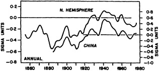
FIGURE 1
Time series of normalized annual mean surface air temperature averaged over China and the entire Northern Hemisphere. (After Bradley et al., 1987; reprinted with permission of Springer-Verlag.)
-
Is the zonally averaged temperature signature associated with the El Niño/Southern Oscillation (ENSO) largely a tropical phenomenon, or is it felt globally?
-
Are the interdecadal trends in surface air temperature and temperatures aloft virtually identical, or is there evidence of systematic trends in the static stability of the troposphere?
STRUCTURE AND SEASONALITY OF VARIATIONS IN SURFACE AIR TEMPERATURE
The variability of wintertime temperatures over the high-latitude continents (specifically western Canada and Siberia) is substantially larger than anywhere else in the hemisphere, and anomalies in these two regions are influenced by the Pacific-North American (PNA) teleconnection pattern (Gutzler et al., 1988). Wintertime and springtime warming over these regions has been implicated in the recent rise in the mean surface air temperature during the 1980s (Trenberth, 1990; Folland et al., 1990, 1992; Jones and Briffa, 1992). Indeed, the spatial signature of the PNA pattern is clearly evident in the field of 1,000 to 500 hPa thickness anomalies for the 1980s, shown in Figure 2. Comparison of the wintertime mean and the more bland annual mean fields in Figure 2 suggests that this regional pattern is largely a wintertime phenomenon.
Lest the significance of the high-latitude continents be overstated, it should be noted that trends in the PNA pattern and wintertime temperatures over the high-latitude continents do not always determine the sign of the trend in the mean surface air temperature over the Northern Hemisphere. A notable example is the period of the late 1950s and early 1960s, when the mean temperature of the Northern Hemisphere extratropics fell slightly, even though wintertime temperatures over western Canada rose substantially in connection with a reversal in the predominant polarity of the PNA pattern (van Loon and Williams, 1976; Wallace and Zhang, 1993).
Perhaps as a result of regional features such as the PNA
TABLE 1 Temporal Correlation Between Area-Weighted, Normalized Seasonal-Mean Surface-Air Temperature over China, and All Northern Hemisphere Land Masses (after Bradley et al., 1987)
|
|
Spring |
Summer |
Autumn |
Winter |
Annual |
|
Unsmoothed data |
0.66 |
0.67 |
0.68 |
0.54 |
0.81 |
|
Smoothed (as in Figure 1) data |
0.92 |
0.93 |
0.90 |
0.68 |
0.95 |
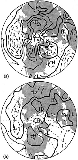
FIGURE 2
Difference in thickness of the 1000-500 hPa layer, 1981-1990 minus the period 1951-1980. (a) Wintertime means, (b) annual means. Contour interval 10 m (0.5K). Negative values are dashed. (After Wallace et al., 1993; reprinted with permission of the American Meteorological Society.)
pattern, local wintertime temperatures generally tend to be less coherent with the mean temperature of the Northern Hemisphere than those observed during other seasons. For example, in the EOF analysis of Barnett (1978) cited in the previous section, the leading mode of wintertime surface air temperature is dominated by regional-scale features reminiscent of the PNA pattern, in sharp contrast to the monopolar structure of the leading mode of annual mean temperature. And when the annual mean time series shown in Figure 1 are broken down by season (Table 1), strong positive correlations are observed between the China series and the hemispheric mean series for every season except winter.
Since the low-frequency variability during the warm season is less strongly influenced by circulation anomalies, hemispheric mean temperatures observed during the warm season should be of particular interest from the standpoint of detecting thermodynamically induced hemispheric or global trends. Seasonal mean time series of hemispheric mean surface air temperature presented by Jones and Briffa (1992) are suggestive of a more favorable "signal-to-noise ratio" for the detection of interdecadal variability in the plots for the warm season. This distinction is brought out clearly in Figures 3 and 4, which show time series of monthly mean surface air temperature anomalies averaged over the extratropical Northern and Southern Hemispheres,3 respectively, with the months May to October and November to April plotted separately. These figures, and several of the subsequent figures in this paper, are based on the data set compiled by Jones et al. (1985, 1986a) under the sponsorship of the U.S. Department of Energy. The "DOE" identifier on individual curves also refers to these data. Analogous plots (not shown) based on 3-month means (May-through-July and August-through-October versus November-through-January and February-through-April) also exhibit substantially more scatter during the cold seasons.
Hence, it can be concluded that the recent upward trend in surface air temperature averaged over the Northern Hemisphere is a reflection of a genuine, year-round hemispheric warming. The more dramatic rises in wintertime temperatures over western Canada and Siberia are of considerable interest in their own right, but it seems unlikely that they are the fundamental cause of the hemispheric warming, which shows up just as clearly in the warm-season time series as in the cold-season time series.
The choice of how to define the hemispheric averages in Figures 3 and 4 is, of course, rather arbitrary. In this particular case it does not make much difference whether one considers the entire hemisphere, the extratropics poleward of 20° latitude, or a smaller polar-cap region. As one moves the outer boundary poleward, the interdecadal trends become somewhat larger, but so does the sampling noise associated with regional and short-term variability, so one's overall impression of the "signal-to-noise ratio" does not change a great deal.
THE SIGNAL OF EL NIÑO/SOUTHERN OSCILLATION IN THE GLOBAL TEMPERATURE FIELD
Walker and Bliss (1932) showed that their Southern Oscillation Index (SOI)4 modulates surface air temperature, averaged over the tropics, as well as over certain regions of higher latitudes, such as southwestern Canada. This result was confirmed by the later studies of Newell and Weare (1976), Angell and Korshover (1978), Newell (1979), and Horel and Wallace (1981), which showed that the ENSO signature is evident in time series of mean tropical tropospheric temperature, lagged by about a season or two relative to sea surface temperatures in the equatorial Pacific. This effect is clearly evident in time series of the radiance in Channel 2 of the MSU carried aboard the TIROS satellites (an indicator of the mean temperature of the 1,000 to 300 hPa layer) shown in Figure 5. The upper time series is unsmoothed monthly mean sea surface temperature (SST) averaged over the equatorial Pacific from 160°E to the South American coast and from 5°N to 5°S, which shows clearly the signature of the three most recent warm episodes (19821983, 1986-1988, and 1991-1992). The corresponding MSU-2 time series, averaged over the latitude belt from 20°S to 20°N shown just below it, exhibits the same features, some of them lagged by about a season, as noted in the studies cited above. A remarkably similar signature is evident in the mean surface air temperature of the tropics based on gridded data from land stations, shown in the lowest curve. The much larger amplitude of the SST time series and the phase lag between SST and the other time series are consistent with the notion that the ENSO signature in tropical tropospheric temperature is a forced response to local perturbations in the heat balance at the air-sea interface in the equatorial eastern Pacific. The fact that the ENSO signature is virtually identical in the MSU-2 and land-
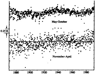
FIGURE 3
Scatterplot of the time series of monthly mean surface air temperature anomalies, averaged over all land gridpoints in the Northern Hemisphere extratropics (25° to 90°), based on the U.S. Department of Energy data set, plotted separately for the calendar months May to October and November to April, as indicated. One small tick mark on the vertical scale is equivalent to 0.5K.
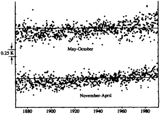
FIGURE 4
Temperature anomaly time-series scatterplot as in Figure 3, but for the Southern Hemisphere extratropics.
surface temperature time series, but slightly larger in the former, suggests that it is transmitted from the equatorial Pacific to the remainder of the tropics via thermally direct circulations in the free atmosphere.
A strong correspondence between equatorial Pacific SST and surface air temperature averaged over the tropical belt is also evident in the longer time series shown in Figure 6. Because of the slight phase lag between the SST anomalies and the land-surface temperature anomalies, the correlation coefficient between the two time series is only about 0.5; nonetheless, the correspondence between warm and cold phases of the ENSO cycle and tropical tropospheric
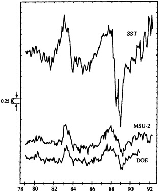
FIGURE 5
Three time series. Upper series: equatorial Pacific sea surface temperature anomalies for the region 160°E to 90°W, 5°N to 5°S, which corresponds to the regions included in Niño 3 and Niño 4 in the Climate Diagnostic Bulletin. Middle series: tropospheric temperature anomalies, as sensed by the Microwave Sounding Unit (MSU-2) carried aboard the TIROS N satellites, averaged over the tropical belt (20°N to 20°S). Lower series: surface air temperature over all land grid points within the tropical belt (20°N to 20°S). The temperature scale is the same for all three curves: one small tick mark is equivalent to 0.25K. MSU data courtesy of Roy Spencer, NASA Marshall Space Flight Center, Huntsville, Ala.. (After Yulaeva and Wallace, 1994; reprinted with permission of the American Meteorological Society.)
temperature anomalies is unmistakable. A correlation coefficient of about 0.8 can be obtained by performing a transformation on the SST time series, using it as the input for a stochastically forced climate model based on the formulation of Hasselmann (1976) (see also Frankignoul, 1985, Eq. 20). This formulation contains only two free parameters. One is analogous to a characteristic damping time of the forced climate system, which can be determined from the Stefan-Boltzmann Law, under the assumption that tropospheric temperature anomalies are radiatively damped. The other is analogous to a heat capacity (in this case, that of the troposphere and perhaps some part of the oceanic mixed layer in the passive regions of the tropics). This coefficient can be determined empirically to optimize the agreement between the output of the model and the tropospheric time series. The output of the model, shown as the middle curve in Figure 6, captures most of the features in the land-surface temperature time series immediately above it. For further details, see Yulaeva and Wallace (1994).
Vestiges of the same warm and cold episodes are evident in global mean MSU-2 time series shown in Figure 7, but the ENSO signal is diluted by about a factor of 3 by being combined with unrelated features in the extratropical time series, which are also shown in the figure. Time series of 850 to 300 hPa thickness based on zonal averages of longer records of rawinsonde observations for selected latitude belts also give the impression that the ENSO signal is largely confined to the tropical belt (Angell, 1988). It is evident from Figure 7 that the interannual variability of tropical tropospheric temperatures in association with the ENSO cycle is much larger than that of extratropical tropospheric temperatures. One obtains similar impressions from the results of EOF analysis of cosine-weighted, zonally averaged temperature anomalies derived from MSU-2 instruments. The leading mode is largely confined to the tropics and symmetric about the equator (Yulaeva and Wallace, 1994).
Figure 8 shows longer records of land surface air temperature for the same latitude belts. As in the previous figure, the temperature scales for all four curves are the same, but in this case a 3-month running mean filter has been applied to suppress the high-frequency variability in the extratropi-
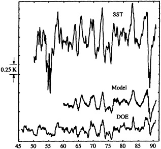
FIGURE 6
Time series of (upper) equatorial Pacific SST, as in Figure 5, (lower) surface air temperature over all land gridpoints within the tropical belt (20°N to 20°S), and (middle) simulated tropical tropospheric response to the SST time series, based on a simple thermodynamic model as described in Yulaeva and Wallace (1994). One small tick mark on the vertical scale is equivalent to 0.5K.
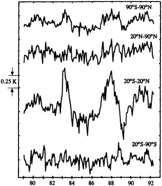
FIGURE 7
Tropospheric temperatures based on the MSU-2 data averaged over the entire globe, the extratropical Northern Hemisphere (poleward of 20°N), the tropical belt 20°S to 20°N, and the extratropical Southern Hemisphere (poleward of 20°S). The temperature scale is the same for all four curves: one small tick mark is equivalent to 0.25K. (After Yulaeva and Wallace, 1994; reprinted with permission of the American Meteorological Society.)
cal time series. The relationships pointed out in the previous paragraph appear to be valid during earlier decades. In particular, note the weak coupling between the tropical and extratropical time series on the interannual time scale.
It has been suggested that the prevalence of the warm phase of the ENSO cycle during the late 1970s and 1980s has contributed to the global warming observed during this period (e.g., see Trenberth, 1990; Trenberth and Hurrell, 1995). Inspection of Figure 8 suggests that some of the warming observed within the tropical belt from the late 1970s onward could be attributed to the absence of a well-defined cold phase of the ENSO cycle between 1976 and 1987. On the other hand, this feature could equally well be interpreted as a gradual upward temperature trend that is independent of the ENSO variability. The latter interpretation is supported by the fact that equatorial Pacific SST (Figure 6) was substantially colder during 1988 than at any time since the early 1950s, yet tropical land-surface temperatures (Figure 8), although cool relative to other periods during the 1980s, were not as cool as those observed on a number of occasions during the 1960s and early 1970s.
The time series of extratropical Northern and Southern
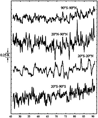
FIGURE 8
Land-surface temperatures based on the DOE data set averaged over the entire globe, the extratropical Northern Hemisphere (poleward of 20°N), the tropical belt 20°S to 20°N, and the extratropical Southern Hemisphere (poleward of 20°S). The temperature scale is the same for all four curves: one small tick mark is equivalent to 0.25K.
Hemisphere surface air temperature in Figure 8 are not particularly well correlated with one another. The only common element is the upward trend during the past decade. Since the ENSO signal is common to the northern and southern tropics, it contributes to the correlation between the two hemispheres when the spatial average is extended all the way to the equator, as in many published time series (e.g., Spencer and Christy, 1992, Figure 12). It is evident from our figure that when the tropical belt is excluded in defining the hemispheric means, the correlation between the hemispheric time series drops dramatically.
Hence, we can conclude that the interannual variations in zonally averaged temperature associated with the ENSO cycle are largely restricted to the tropics, even though the ENSO signal is apparent in global mean temperature.
TRENDS IN SURFACE-AIR TEMPERATURE VERSUS TEMPERATURES ALOFT
Low-frequency variability in temperatures aloft over the extratropical Northern Hemisphere exhibits the same type of structural characteristics and seasonality as variability in
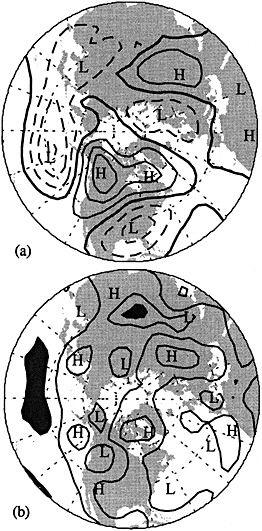
FIGURE 9
Leading EOFs of (a) wintertime (December to February) and (b) summertime (June to August) mean hemispheric (poleward of 20°N) 1000-500 hPa thickness field based on NMC analyses for the period 1946 to 1989, scaled such that they represent the thickness perturbations corresponding to an amplitude of unity for the corresponding expansion coefficient contour interval 0.2. Negative values are dashed; regions of negative values are shaded in the lower panel. The numbers at the upper right are the percentages of the hemispherically integrated variance explained by that mode. Courtesy of Yuan Zhang, Department of Atmospheric Sciences, University of Washington.
temperatures at the earth's surface (Wallace et al., 1993). The wintertime variability of the 1,000 to 500 hPa thickness field, a measure of the mean temperature of the lower troposphere, is dominated by a PNA-like pattern (Figure 9, upper panel). The summertime variability is dominated by a relatively featureless ''background field" (Figure 9, lower panel) whose expansion coefficient is highly correlated with the time series of hemispheric mean thickness. Even though the wintertime mode exhibits higher amplitude, the leading EOF of annual mean thickness closely resembles the leading summertime pattern, which explains a higher percentage of the hemispherically integrated variance than its wintertime counterpart, and is evidently present year round. For fluctuations with periods of 5 years or longer, variations in hemispheric mean thickness account for half the hemispherically integrated variance of the local thickness time series.
There is some evidence of systematic differences in the long-term trends in surface air temperature versus temperatures aloft. Figure 10 compares hemispherically averaged temperature time series based on (a) surface air temperature over land, (b) mean tropospheric temperature as sensed by Channel 2 of the MSU, and (c) mean virtual temperature of the 1,000 to 500 hPa layer based on the operational analyses of the National Meteorological Center (NMC), all for the area poleward of 20°N. All three time series have been smoothed by taking 3-month running means, and the DOE climatology has been adjusted to eliminate the annual march in the 1979 to 1990 period of record. Neither of the upper-air time series exhibits as pronounced a warming trend as that evident in the time series of surface air temperature, nor do the hemispheric mean time series of Angell (1988) or Oort and Liu (1993), which are based on radiosonde data. The corresponding MSU-2 time series of
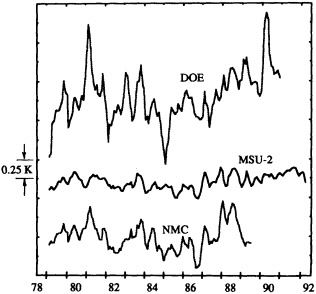
FIGURE 10
Time series of 3-month running means of (upper) surface air temperature over land, based on the DOE data set, (middle) tropospheric temperature based on MSU-2, and (lower) mean virtual temperature of the 1000-500 hPa layer based on the NMC operational analyses, all averaged over the Northern Hemisphere poleward of 20°N. The climatology for the DOE data is based on the 1979-1990 reference period. The temperature scale is the same for all three curves: one small tick mark is equivalent to 0.25K.
tropospheric temperature in the extratropical Southern Hemisphere also fails to reproduce the pronounced warming that is evident in the surface air temperature record, as shown in Figure 11.
Figure 12 shows a comparison of the same surface air temperature and NMC upper-air temperature time series for the extratropical Northern Hemisphere, based on a longer period of record. Other discrepancies are evident around 1955 and 1963, when the mean 1,000 to 500 hPa temperature in the NMC analyses dropped substantially, while the surface temperatures cooled by a lesser amount. Lambert (1990) has suggested that both these features are reflections of changes in analysis procedures, while Shabbar et al.
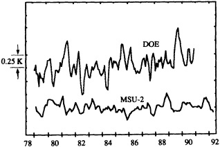
FIGURE 11
Series as in the two top curves of Figure 10, but for the Southern Hemisphere poleward of 20°S. The temperature scale is the same for both curves: one small tick mark is equivalent to 0.1K.
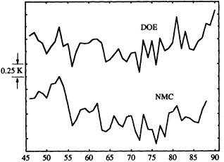
FIGURE 12
Series as in the top and bottom curves in Figure 10, but of annual means based on the calendar year. The temperature scale is the same for both curves: one small tick mark is equivalent to 0.25K.
(1990) have linked the second to a change in climate regimes.
There are many reasons to be suspicious of the sharp downward temperature trend during the late 1950s and early 1960s indicated by the NMC analyses. Changes in radiosonde sensors, reporting times, and analysis procedures that occurred during this period could have introduced spurious trends or discontinuities in the record. Yet in view of the marked differences between temperature trends in the MSU-2 and DOE data sets during the 1980s, it would be imprudent to dismiss the possibility that the cooling aloft might have been somewhat more pronounced than that at the earth's surface. A tendency toward stronger cooling aloft than at the surface would be indicative of a long-term decrease in the stratification of the lower troposphere.
A contributing factor may be the shift in the predominant polarity of the wintertime PNA pattern between the early 1950s and the 1980s. This change was marked by cooling of several degrees aloft over the North Pacific and warming by a comparable amount at the earth's surface over western Canada and much of Siberia (Gutzler et al., 1988; Wallace et al., 1993). Since this effect was observed only during the cold season over limited regions of the hemisphere, it seems unlikely that it could be the main reason for the difference between the time series of surface air temperature and temperatures aloft over the Northern Hemisphere. Of course, it also would not account for the difference between the recent temperature trends in the MSU-2 and DOE time series in the Southern Hemisphere, which is in the same sense.
A downward trend in static stability is also suggested by the marked difference between the long-term trends in daily maximum and daily minimum temperatures since the 1940s (Plantico et al., 1990; Karl et al., 1995). Minimum temperature exhibits a pronounced upward trend relative to maximum temperature, resulting in a decrease of several percent in the mean diurnal temperature range during this period of record. The decrease is observed during all seasons and over most geographical regions. Higher daily minimum surface air temperatures could be an indication of weaker nighttime inversions, which would contribute to a decrease in the mean static stability of the lower troposphere.
LOWER STRATOSPHERIC TEMPERATURE
Figure 13 shows the time series of lower stratospheric temperatures based on Channel 4 of the MSU, whose level of unit optical depth is near 70 hPa. The global curve is the same as the one published by Spencer and Christy (1993). Consistent with earlier studies based on radiosonde data (Newell, 1970; Angell and Korshover, 1978), it shows distinct signatures of the two major volcanic eruptions during this period (El Chichon in April 1982 and Pinatubo in June 1991) whose plumes reached stratospheric levels. The
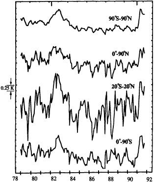
FIGURE 13
Time series of lower stratospheric temperature anomalies, relative to the 1979-1991 reference period, as sensed by the stratospheric channel of the microwave sounding unit (MSU4). Curves show the average over the entire globe, the average over the Northern Hemisphere (0° to 90°N), the average over the tropics (20°N to 20°S), and the average over the Southern Hemisphere (0° to 90°S). The times of the El Chichon and Pinatubo eruptions are indicated near the top of the figure. One small tick mark on the vertical scale is equivalent to 0.25K. Data courtesy of Roy Spencer, NASA Marshall Space Flight Center, Huntsville, Ala. (After Yulaeva et al., 1994; reprinted with permission of the American Meteorological Society.)
volcanic signature shows up much more clearly in the globally averaged time series than in the time series for the tropical belt or for individual hemispheres. Over a wide range of frequencies, much of the large, dynamically induced temperature variability involves compensating warming and cooling in different latitude belts. For example, the correlation between month-to-month temperature changes in the tropics (20°N to 20°S) and extratropics is -0.79 (-0.86 when the 3 months subsequent to the Pinatubo eruption are excluded). The dynamically induced temperature perturbations are almost entirely filtered out by the global averaging, leaving only the smaller radiatively induced perturbations (Yulaeva et al., 1994).
During the period of record 1979 through 1992, the globally averaged MSU-2 and MSU-4 time series are virtually uncorrelated. In the presence of the large ENSO signal in tropospheric temperatures, the cooling signatures associated with the El Chichon and Pinatubo eruptions do not stand out clearly in Figures 5 and 7. As pointed out by Bradley (1988) and Mass and Portman (1989), the Katmai eruption in the Aleutians in June 1912 was followed by a pronounced dip in Northern Hemisphere monthly mean temperatures during the warm season (Figure 3, upper plot). There was an analogous, although somewhat weaker, dip following the eruption of Ksudach (also in the Aleutians) three years earlier. There is no clear signature of the ENSO cycle in the global-mean stratospheric time series, although Randel and Cobb (1994) and Yulaeva and Wallace (1994) have shown evidence of a geographically localized signature.
DISCUSSION
The ENSO and volcanic signatures are reflections of natural variability in the earth system: The former is generated by processes within the more limited atmosphere-ocean climate system, and the latter is externally forced. The remaining variability in the climate record is predominantly interdecadal in time scale. It is not clear how much of it is due to natural causes and how much is a consequence of anthropogenic influences. Depending on whether aerosols or greenhouse gases predominate, and the strength and polarity of various feedbacks, anthropogenic influences might serve either to warm or to cool the troposphere. Hence, the absence of a pronounced upward trend in tropospheric temperatures as sensed by the MSU-2 instrument during the past decade does not necessarily preclude the possibility that a detectable anthropogenic signal exists. A gradual increase in the optical thickness of the atmosphere is, in fact, suggested by the secular decrease in static stability observed over the course of the past 40 years in the Northern Hemisphere extratropics and over at least the past decade in the Southern Hemisphere extratropics, coupled with the marked increase in nighttime temperatures relative to daytime temperatures at many land stations. Increases in greenhouse gases and aerosols could both be contributing in the same sense to these trends. Such a signature would be consistent with the results of many general-circulation models' simulations of the response to increasing CO2, which show the largest temperature rises at the earth's surface at higher latitudes, in regions subject to frequent low-level temperature inversions.
The sharp rise in Northern Hemisphere surface air temperatures from 1920 to 1940 (Figures 3 and 4) coincided with a northward shift of the Gulfstream (Bjerknes, 1959; Deser and Blackmon, 1995). The subsequent dip during the 1960s and 1970s may be related to a reduction in the salinity of the surface waters of the subpolar North Atlantic that was observed during this period (Dickson et al., 1988; Delworth et al., 1995; Dickson, 1995; Mysak, 1995), which might have tended to suppress the thermohaline circulation,
thereby reducing the poleward heat transport. It has also been suggested that increasing concentrations of sulfate aerosols over the Northern Hemisphere might have been responsible for the cooling during that period (Charlson et al., 1991, 1992). Hence, there is no shortage of mechanisms that may have contributed to the observed interdecadal variability in the climate record. The problem is to quantify the arguments, through the use of climate models, so that the dominant mechanisms can be identified (Battisti, 1995; Rind and Overpeck, 1995).
The results presented in the foregoing sections serve to illustrate the need for a flexible, pragmatic approach toward the smoothing of monthly mean data, and stratifying of data by season and by latitude belt. For example, in displaying tropospheric data, a three-way partitioning into means for the tropics and Northern and Southern Hemisphere extratropics appears to be more informative than the more commonly used two-way partitioning by hemisphere, because it isolates the tropical ENSO signal. For stratospheric data it may be best not to do any partitioning at all, since global averaging tends to filter out spurious, dynamically induced temperature fluctuations.
ACKNOWLEDGMENTS
I would like to thank Yuan Zhang and Elena Yulaeva for providing material from their graduate research projects, and Clifford Watson for assistance with the preparation of the figures. Clifford Mass offered a number of helpful comments. The work was supported by the National Science Foundation under Grant 9215512.
Commentary on the Paper of Wallace
HENRY F. DIAZ
NOAA/Environmental Research Laboratories
Before we begin a discussion, I just want to encapsulate some of the primary conclusions or at least principal points Dr. Wallace discussed. First, I think that the ENSO is manifested primarily in tropical temperatures. When you look at global indices or hemispheric indices, what you are seeing is essentially the folding of the tropical signal into the overall record. A very important point that we should consider in the context of the previous talks and the slides that Professor Lindzen showed is that the volcanic temperature signal on the hemispheric temperature record is relatively short-lived. It seems to me that we are talking about thermal relaxation on the order of 3 to 5 years from the time when a major volcanic eruption takes place, through the drop in the temperatures, to the recovery. In that sense, I think that we are not talking about decades but less than a decade.
The volcanic effect also says something about the sensitivity of climate to greenhouse perturbations. There is something interesting about the difference between the Northern and Southern Hemispheres' temperature responses. Even in the 1979-to-present record, the atmospheric response is quite rapid, and there are clear differences between the two hemispheres. We should try to discover whether they are due primarily to the fact that the Southern Hemisphere reflects the ocean damping effects, and whether the Antarctic ice cap has something to do with the difference. Also, the lower stratosphere has a much more spatially homogenous response than the troposphere, and perhaps long-term monitoring of lower stratospheric temperatures would turn out to be a useful tool. Large temperature changes in the lower stratosphere have been projected, and I think we should consider how the observations and the predictions are coming together.
Dr. Wallace mentioned that interdecadal temperature signals are different for surface and upper air indices. This is suggested by data for the last decade, although the record is not really long enough that we can say so with certainty. The correlation between, say, Jim Angell's 63-station radiosonde network and temperatures at the surface is sufficiently high to explain about 50 percent of the variance. For comparison, the correlation between that radiosonde network and the MSU data is about 0.8 or higher.
Discussion
TRENBERTH: Let me comment a moment on the trend aspect of our analysis of the MSU data. Our paper comparing it with the IPCC data set for surface temperature will be in the September issue of the Journal of Climate, by the way. Over North America, the MSU Channel 2 data has about 0.2°C per decade less trend than the surface record. My best guess is that this results from the way in which all the differences between the satellites getting the TOVS series of data are taken out.
WALLACE: That indeed is a point to be taken seriously, but I don't think we should dismiss the possibility that these differences might prove to be real. Another five years of data should settle the matter.
TRENBERTH: Yes, that's true; there are real physical differences. Over North America the correlation is better than 0.9, whereas over the rest of the world it's not that good.
SHUKLA: I had the impression from various Oort papers that a large part of the vertically integrated three-dimensional temperature for the Northern Hemisphere is the ENSO signal.
WALLACE: Yes, I think his results are consistent with what I have indicated—that the ENSO signal shows up clearly in the globally averaged temperature time series, but not in the time series for extratropical latitudes.
KAROLY: I've actually performed a correlation of SST with upper-air temperatures, stratified by latitude and elevation. It's very strong up to 25° north and south, being dominated by direct tropical SST, but between 25° and the poles you get structures that vary in sign in different latitude bands, and the correlation is negligible.
RASMUSSON: What about the differences between land and sea surface temperatures, though both seem to have been increasing in the last couple of decades?
WALLACE: The low-frequency interdecadal trends exhibit the same signature in land-based and marine data sets, as can be seen from the IPCC report's figures. But I suspect that those two data sets show quite different scatter around the trend lines for individual months or seasons, year by year. I think that if you found a point in the time series for land that was way below the trend line, the corresponding one for the marine series would be way above the trend line.
RASMUSSON: Different parts of the ocean certainly have different temporal responses; the tropical temperatures have ramped up very quickly since the mid-1970s.
LINDZEN: I think you made a crucial point, Mike, about the difference between detection and interpretation. For example, data reflecting crustal movement languished for years before the concept of plate tectonics gave them meaning. Also, when we talk about detection, we should be careful not to equate detection of CO2 increase with detection of climate change. Some of the measures of CO2 change have to do with radiative flux, which varies strongly with the time of day. Also, one thing I would very much like to see done is further work comparing measurements made at surface level with those made at 500 millibars, particularly as regards lapse-rate variability. Some of Oort's recent work suggests that surface temperature changes are amplified at 500 mb globally, while some of the MSU data indicate that the integral changes over a certain region may be reduced.
KEELING: As I remember, Oort found a substantial signal, about 6 months delayed from the tropical signal, at 200 mb, which he used as a proxy for integrated temperature.
KAROLY: There is a very strong 200-mb signal, but if you average around the hemisphere the latitudinally averaged signal in the extratropics is weak.
GHIL: I'd like to make two remarks. The first is about the spatial patterns. It's quite clear that signals such as the so-called ENSO interannual signal have associated spatial patterns. Since this signal is relatively homogeneous throughout the tropics, which is a large part of the globe, it will dominate any global average. Also, spatial patterns of various signs outside the tropics are going to cancel each other out if you do zonal averages.
My second remark relates to Dick Lindzen's point about the volcanic signal and its two-part decay. Mike showed us clusters of colder months that disappeared after a year or two, that being the fast-decay part. I wonder whether interdecadal variability might not be masking the slow-decay part.
RIND: It would be interesting to clarify the nature of the system's long response time. A volcanic eruption is such a quick signal that you might observe a much shorter response than a system with so many feedbacks would otherwise exhibit; the longer responses could be drowned in the rest of the variability.
TRENBERTH: I'd like to pick up on one of Michael Ghil's points. The Pacific is not in fact coherent with the ENSO signal; the western Pacific tends to have a sign opposite to the eastern Pacific's. The tropics are not necessarily a coherent whole either. However, the ENSO signal is so large in the eastern Pacific that it is twice as high as the standard deviation and four times or more the variance.
WALLACE: There's more on this issue in my paper, but for the purposes of this discussion, I think the tropics can be divided into the 'active' eastern Pacific, where SST is directly influenced by equatorial upwelling, and the 'passive' remainder. I think the ENSO signal is also present, with smaller amplitude and lagged by about a season, in the passive region. Furthermore, I believe that stations in that region, which includes nearly all the land stations in the DOE data set, all exhibit very similar ENSO-related time variability.
We have performed some experiments with a thermodynamic model of the type used by Klaus Hasselmann. With this simple model you can transform an SST time series that is representative of the active region into a time series that looks a lot like the DOE time series for the tropical land stations. So I believe the relationship between the interannual temperature variabilities in different parts of the tropics is much simpler than those for other variables like precipitation and cloudiness.
GROISMAN: I wanted to say that I completely agree that there has to be more than one decay time, and neither the initial decay time nor a sustained signal is an acceptable approximation of the long decay times. And second, don't forget how much global temperature variance differs by season. And sometimes just a change in the Y-axis scale will make a trend look good.
WALLACE: It's only the shorter-term variability—the "noise"— that's larger in winter; the interdecadal component appears to be the same for both. That's why the scatter plots for the summer months look better.
Atmospheric Modeling Reference List
Adem, J. 1964. On the physical basis for the numerical prediction of monthly and seasonal temperatures in the troposphere-ocean-continent system. Mon. Weather Rev. 92:91-104.
Allen, M.R., and L.A. Smith. 1994. Investigating the origins and significance of low-frequency climate modes of variability. Geophys. Res. Lett. 21:883-886.
Anderson, R.Y. 1992. Possible connection between surface winds, solar activity and the Earth's magnetic field. Nature 358:51-53.
Andrews, D.G., C. Leovy, and J.R. Holton. 1987. Middle Atmosphere Dynamics. Academic Press, Orlando, Florida, 489 pp.
Angell, J.K. 1988. Variations and trends in tropospheric and stratospheric global temperature, 1958-87. J. Climate 1:1296-1313.
Angell, J.K., and J. Korshover. 1978. Estimate of global temperature variations in the 100-30 mb layer between 1958 and 1977. Mon. Weather Rev. 106:1422-1432.
Baldwin, M.P., and T.J. Dunkerton. 1989. Observations and statistical simulations of a proposed solar cycle/QBO/weather relationship. Geophys. Res. Lett. 16:863-866.
Baliunas, S., and R. Jastrow. 1990. Evidence for long-term brightness changes of solar-type stars. Nature 348:520-523.
Barnett, T.P. 1978. Estimating variability of surface temperature in the northern hemisphere. Mon. Weather Rev. 106:1353-1367.
Barnett, T.P. 1986. Detection of changes in the global tropospheric temperature field induced by greenhouse gases. J. Geophys. Res. 91:6659-6667.
Barnett, T. 1991. An attempt to detect the greenhouse-gas signal in a transient GCM simulation. In Greenhouse-Gas-Induced Climatic Change: A Critical Appraisal of Simulations and Observations. M.E. Schlesinger (ed.). Elsevier, Amsterdam, pp. 559-568.
Barnett, T.P., A.D. Del Genio, and R. Ruedy. 1992. Unforced decadal fluctuations in a coupled model of the atmosphere and ocean mixed layer. J. Geophys. Res. 97:7341-7354.
Barnola, J.M., D. Raynaud, Y.N. Korotkevitch, and C. Lorius. 1987. Vostok ice-core provides 160,000-year record of atmospheric CO2. Nature 329:408-414.
Barnston, A.G., and R.E. Livezey. 1989. A closer look at the effect of the 11-year solar cycle and the quasi-biennial oscillation in the Northern Hemisphere 700 mb height and extra tropical North American surface temperature. J. Climate 2:1295-1313.
Battisti, D.S. 1995. Decade-to-century time-scale variability in the coupled atmosphere-ocean system: Modeling issues. In Natural Climate Variability on Decade-to-Century Time Scales. D.G. Martinson, K. Bryan, M. Ghil, M.M. Hall, T.R. Karl, E.S. Sarachik, S. Sorooshian, and L.D. Talley (eds.). National Academy Press, Washington, D.C.
Beer, J., U. Siegenthaler, G. Bonani, R.C. Finkel, H. Oeschger, M. Suter, and W. Wolfli. 1988. Information on past solar activity and geomagnetism from "Be in the Camp Century ice core". Nature 332:675-679.
Bell, T.L. 1982. Optimal weighting of data to detect climatic change: Application to the carbon dioxide problem. J. Geophys. Res. 87:11161-11170.
Bell, T.L. 1986. Theory of optimal weighting of data to detect climatic change. J. Atmos. Sci. 43:1694-1710.
Bjerknes, J. 1959. The recent warming of the North Atlantic. In Atmosphere and Sea in Motion, the Rossby Memorial Volume. B. Bolin (ed.). Rockefeller Inst. Press in association with Oxford Press, New York, pp. 65-73.
Blanford, H.F. 1891. The paradox of the sun-spot cycle in meteorology. Nature 43:583-587.
Bloomfield, P., and D. Nychka. 1992. Climate spectra and detecting climatic change. Climatic Change 22:275-288.
Bradley, R.S. 1988. The explosive volcanic eruption signal in northern hemisphere continental temperature records. Climatic Change 12:221-243.
Bradley, R.S. 1990. Pre-instrumental climate: How has climate varied during the past 500 years? In Greenhouse Gas-Induced Climatic Change: A Critical Appraisal of Simulations and Observations. M. Schlesinger (ed.). Elsevier, Amsterdam, pp. 391-412.
Bradley, R.S. 1992. Instrumental records of past global change: Lessons for the analysis of noninstrumental data. In Global Changes of the Past. R.S. Bradley (ed.). UCAR/Office of Interdisciplinary Earth Studies, Boulder, Colo., pp. 103-116.
Bradley, R.S., and P.D. Jones (eds.). 1992a. Climate Since A.D. 1500. Routledge, New York, 679 pp.
Bradley, R.S., and P.D. Jones. 1992b. Records of explosive volcanic eruptions over the last 500 years. In Climate Since A.D. 1500. R.S. Bradley and P.D. Jones (eds.). Routledge, New York, pp. 606-622.
Bradley, R.S., H.F. Diaz, P.D. Jones, and P.M. Kelly. 1987. Secular fluctuations in temperature over northern hemisphere land areas and mainland China since the mid-nineteenth century. In The Climate of China and Global Climate. Ye D., Fu C., Chao J., and M. Yoshino (eds.). China Press and Springer-Verlag, pp. 77-87.
Bray, J.R. 1974. Glacial advance relative to volcanic activity since A.D. 1500. Nature 248:42-43.
Brewer, P.G., W.S. Broecker, W.J. Jenkins, P.B. Rhines, C.G. Rooth, J.H. Swift, T. Takahashi, and R.T. Williams. 1983. A climatic freshening of the deep Atlantic (north of 50°N) over the past 20 years. Science 222:1237-1239.
Broecker, W.S., and G.H. Denton. 1989. The role of ocean-atmosphere reorganizations in glacial cycles. Geochim. Cosmochim. Acta 53:2465-2501.
Broecker, W.S., T.H. Peng, and R. Engh. 1980. Modeling the carbon system. Radiocarbon 22:565-598.
Broecker, W.S., D.M. Peteet, and D. Rind. 1985. Does the ocean-atmosphere system have more than one stable mode of operation? Nature 315:21-26.
Broecker, W.S., M. Andree, W. Wolflie, H. Oeschger, G. Bonani, J. Kennett, and D. Peteet. 1988. The chronology of the last deglaciation: Implications to the cause of the Younger Dryas event. Paleoceanography 3:1-19.
Broomhead, D.S., and G.P. King. 1986. Extracting qualitative dynamics from experimental data. Physica D 20:217-236.
Budyko, M.I. 1969. The effect of solar radiation variations on the climate of the Earth. Tellus 21:611-619.
Cebula, R.P., M.T. DeLand, and B.M. Schlesinger. 1992. Estimates of solar variability using the solar backscatter ultraviolet (SBLTV) 2 Mg 11 Index from the NOAA 9 satellite. J. Geophys. Res. 97:11613-11620.
Cess, R.D. 1976. Climate change: An appraisal of atmospheric feedback mechanisms employing zonal climatology. J. Atmos. Sci. 33:1831-1843.
Charlson, R.J., J. Lagner, H. Rodhe, C.B. Leovy, and S.G. Warren. 1991. Perturbations of the northern hemisphere radiative balance by backscattering from anthropogenic sulfate aerosols. Tellus 43AB:152-163.
Charlson, R.J., S.E. Schwartz, J.M. Hales, R.D. Cess, J.A. Coakley Jr., J.E. Hansen, and D.J. Hofmann. 1992. Climate forcing by anthropogenic aerosols. Science 255:423-430.
Charney, J.G., and J.G. DeVore. 1979. Multiple flow equilibria in the atmosphere and blocking. J. Atmos. Sci. 36:1205-1216.
Cole, J.E. 1992. The spectrum of recent variability in the southern oscillation: Results from a Tarawa atoll coral . Ph.D. Thesis, Columbia University, 302 pp.
Cole, J.E., D. Rind, and R. Fairbanks. 1992. Isotopic responses to climate variability in the GISS GCM: Interannual vs. glacial/ interglacial mechanisms. EOS, spring supplement (abstract), p. 151.
Cook, E.R., B.M. Buckley, and R.D. D'Arrigo. 1995. Interdecadal temperature oscillations in the Southern Hemisphere: Evidence from Tasmanian tree rings since 300 B.C. In Natural Climate Variability on Decade-to-Century Time Scales. D.G. Martinson, K. Bryan, M. Ghil, M.M. Hall, T.R. Karl, E.S. Sarachik, S. Sorooshian, and L.D. Talley (eds.). National Academy Press, Washington, D.C.
Cooper, N.S., K.D.B. Whysall, and G.R. Bigg. 1989. Recent decadal climate variations in the tropical Pacific. J. Climate 9:221-242.
Crowley, T.J., and G. North. 1991. Paleoclimatology. Oxford University Press, New York, 339 pp.
Cubasch, U., K. Hasselmann, H. Höck, E. Maier-Reimer, U. Mikolajewicz, B.D. Santer, and R. Sausen. 1992. Time-dependent greenhouse warming computations with a coupled ocean-atmosphere model. Climate Dynamics 8:55-69.
Damon, P.E., and T.W. Linick. 1986. Geomagnetic-heliomagnetic modulation of atmospheric radiocarbon production. Radiocarbon 28:266-278.
Dansgaard, W., S.J. Johnson, H.B. Clausen. D. Dahl-Jensen, N. Gundestirup, C.H. Hammer, and H. Oeschger. 1984. North Atlantic oscillations revealed by deep Greenland ice cores. Geophys. Monogr. 29:288-298.
Delworth, T., S. Manabe, and R.J. Stouffer. 1995. North Atlantic interdecadal variability in a coupled model. In Natural Climate Variability on Decade-to-Century Time Scales. D.G. Martinson, K. Bryan, M. Ghil, M.M. Hall, T.R. Karl, E.S. Sarachik, S. Sorooshian, and L.D. Talley (eds.). National Academy Press, Washington, D.C.
Denton, G.H., and W. Karlen. 1973. Holocene climatic variations—Their pattern and possible causes. Quat. Res. 3:155-205.
Deser, C., and M.L. Blackmon. 1995. Surface climate variations over the North Atlantic Ocean during winter: 1900 to 1989. In Natural Climate Variability on Decade-to-Century Time Scales. D.G. Martinson, K. Bryan, M. Ghil, M.M. Hall, T.R. Karl, E.S. Sarachik, S. Sorooshian, and L.D. Talley (eds.). National Academy Press, Washington, D.C.
de Vries, H. 1958. Variations in concentration of radiocarbon with time and location on Earth. Proc. Koninkl. Nederl. Adak. Wet. Ser B. 61:94-102.
Diaz, H.F., and R.S. Bradley. 1995. Documenting natural climatic variations: How different is the climate of the twentieth century from that of previous centuries? In Natural Climate Variability on Decade-to-Century Time Scales. D.G. Martinson, K. Bryan, M. Ghil, M.M. Hall, T.R. Karl, E.S. Sarachik, S. Sorooshian, and L.D. Talley (eds.). National Academy Press, Washington, D.C.
Dickson, R.R. 1995. The local, regional and global significance of exchanges through the Denmark Strait and Irminger Sea. In Natural Climate Variability on Decade-to-Century Time Scales. D.G. Martinson, K. Bryan, M. Ghil, M.M. Hall, T.R. Karl, E.S. Sarachik, S. Sorooshian, and L.D. Talley (eds.). National Academy Press, Washington, D.C.
Dickson, R.R., J. Meincke, S.A. Malmberg, and A.J. Lee. 1988. The "great salinity anomaly" in the northern Atlantic 1968-82. Prog. Oceanogr. 20:103-151.
Eddy, J.A. 1976. The Maunder Minimum. Science 192:1189-1202.
Enfield, D.B., and S. Luis Cid. 1991. Low-frequency changes in El Niño/Southern Oscillation. J. Climate 4:1137-1146.
Folland, C.K., T.R. Karl, and K.Ya. Vinnikov. 1990. Observed climate variations and change. In Climate Change: The IPCC Scientific Assessment. J.T. Houghton, G.J. Jenkins, and J.J. Ephraums (eds.). Prepared for the Intergovernmental Panel on Climate Change by Working Group I. Cambridge University Press, Cambridge, pp. 195-238.
Folland, C.K., T.R. Karl, N. Nicholls, B.S. Nyenzi, D.E. Parker, and K.Ya. Vinnikov. 1992. Observed climate variability and change. In Climate Change 1992: The Supplementary Report to the IPCC Scientific Assessment. J.T. Houghton, B.A. Callander, and S.K. Varney (eds.). Prepared for the Intergovernmental Panel on Climate Change by Working Group I. Cambridge University Press, Cambridge, pp. 135-170.
Frankignoul, C. 1985. Sea-surface temperature anomalies, planetary waves and air-sea feedbacks in the middle latitudes. Rev. Geophys. 23:357-390.
Friis-Christensen, E., and K. Lassen. 1991. Length of the solar cycle: An indicator of solar activity closely associated with climate. Science 254:698-700.
Gaffin, S.R., M.I. Hoffert, and T. Volk. 1986. Nonlinear coupling between surface temperature and ocean upwelling as an agent in historical climate variations. J. Geophys. Res. 91:3944-3950.
Ghil, M. 1976. Climate stability for a Sellers-type model. J. Atmos. Sci. 33:3-20.
Ghil, M., and S. Childress. 1987. Topics in Geophysical Fluid Dynamics: Atmospheric Dynamics, Dynamo Theory and Climate Dynamics. Springer-Verlag, New York, N.Y., 485 pp.
Ghil, M., and R. Vautard. 1991. Interdecadal oscillations and the warming trend in global temperature time series. Nature 350:324-327.
Ghil, M., M. Kimoto, and J.D. Neelin. 1991. Nonlinear dynamics and predictability in the atmospheric sciences. Rev. Geophys., Supplement (U.S. National Report to the IUGG 1987-1990), pp. 46-55.
Goswami, B.N., and J. Shukla. 1984. Quasi-periodic oscillations in a symmetric general circulation model. J. Atmos. Sci. 41:20-37.
Grove, J.M. 1988. The Little Ice Age. Methuen, London, 498 pp.
Gutzler, D.S., D. Richard, D.A. Salstein, and J.P. Peixoto. 1988. Patterns of interannual variability in the northern hemisphere wintertime 850 mb temperature field. J. Climate 1:949-964.
Halfman, J.D., and T.C. Johnson. 1988. High-resolution record of cyclic climatic change during the past 4 ka from Lake Turkana, Kenya. Geology 16:496-500.
Hansen, A.R., and A. Sutera. 1986. On the probability density distribution of planetary-scale atmospheric wave amplitude. J. Atmos. Sci. 43:
Hansen, J., D. Johnson, A. Lacis, S. Lebedeff, P. Lee, D. Rind, and G. Russell. 1983a. Climatic effects of atmospheric carbon dioxide—A response. Science 220:874-875.
Hansen, J.E., G. Russell, D. Rind, P. Stone, A. Lacis, S. Lebedeff, R. Ruedy, and L. Travis. 1983b. Efficient three-dimensional global models for climate studies: Models I and II. Mon. Weather Rev. 111:609-662.
Hansen, J., A. Lacis, D. Rind, G. Russell, P. Stone, I. Fung, R. Ruedy, and J. Lerner. 1984. Climate sensitivity: Analysis of feedback mechanisms. In Climate Processes and Climate Sensitivity. J.E. Hansen and T. Takahashi (eds.). Geophys. Monogr. Ser. 29:130-163.
Hansen, J., G. Russell, A. Lacis, I. Fung, D. Rind, and P. Stone. 1985. Climate response times: Dependence on climate sensitivity and ocean mixing. Science 229:857-859.
Hansen, J., I. Fung, A. Lacis, D. Rind, S. Lebedeff, R. Ruedy, and G. Russell. 1988. Global climate changes as forecast by Goddard Institute for Space Studies three-dimensional model. J. Geophys. Res. 93:9341-9364.
Hansen, J., A. Lacis, R. Ruedy, and M. Sato. 1992. Potential climate impact of Mount Pinatubo eruption. Geophys. Res. Lett. 19:215-218.
Harvey, L.D.D. 1992. A two-dimensional ocean model for long-term climatic simulations: Stability and coupling to atmospheric and sea ice models. J. Geophys. Res. 97:9435-9453.
Hasselmann, K. 1976. Stochastic climate models. I. Theory. Tellus 28:473-485.
Hasselmann, K. 1979. On the signal-to-noise problem in atmospheric response studies. In Meteorology over the Tropical Oceans. D.B. Shaw (ed.). Royal Meteorological Society, Bracknell, Berkshire, England, pp. 251-259.
Held, I.M., and M.J. Suarez. 1974. Simple albedo feedback models of the icecaps. Tellus 36:613-628.
Hoffert, M.I., and C. Covey. 1992. Deriving global climate sensitivity from paleoclimate reconstructions. Nature 360:573-576.
Hoffert, M.I., A.J. Callegari, and C.-T. Hsieh. 1980. The role of deep sea heat storage in the secular response to climatic forcing. J. Geophys. Res. 85:6667-6679.
Horel, J.D., and J.M. Wallace. 1981. Planetary-scale atmospheric phenomena associated with the Southern Oscillation. Mon. Weather Rev. 109:813-829.
Houghton, D.D., R.G. Gallimore, and L.M. Keller. 1991. Stability and variability in a coupled ocean-atmosphere climate model: Results of 100-year simulations. J. Climate 4:557-577.
Hyde, W., J.T. Crowley, K.-Y. Kim, and G.R. North. 1989. Comparison of GCM and energy balance model simulations of seasonal temperature changes over the past 18000 years . J. Climate 2:864-887.
IPCC. 1990. Climate Change: The IPCC Scientific Assessment. J.T. Houghton, G.J. Jenkins, and J.J. Ephraums (eds.). Prepared for the Intergovernmental Panel on Climate Change by Working Group I. WMO/UNEP, Cambridge University Press, 365 pp.
IPCC. 1992. Climate Change 1992: The Supplementary Report to the IPCC Scientific Assessment. J.T. Houghton, B.A. Callander, and S.K. Varney (eds.). Prepared for the Intergovernmental Panel on Climate Change by Working Group I. WMO/UNEP, Cambridge University Press, 200 pp.
Jenkins, G.M., and D.G. Watts. 1968. Spectral Analysis and its Applications. Holden-Day, San Francisco, 525 pp.
Jones, P.D., and K.R. Briffa. 1992. Global surface air temperature variations over the twentieth century. Part I. Spatial, temporal, and seasonal details. The Holocene 2:165-179.
Jones, P.D., and P.M. Kelly. 1983. The spatial and temporal characteristics of northern hemisphere surface air temperature variations. J. Climatol. 3:243-252.
Jones, P.D., S.C.B. Raper, B.D. Santer, B.S.G. Cherry, C.M. Goodess, P.M. Kelly, T.M.L. Wigley, R.S. Bradley, and H.F.
Diaz. 1985. A Grid Point Surface Air Temperature Data Set for the Northern Hemisphere. Technical Report TR022, U.S. Department of Energy, Carbon Dioxide Research Division, 251 pp.
Jones, P.D., S.C.B. Raper, B.S.G. Cherry, C.M. Goodess, and T.M.L. Wigley. 1986a. A Grid Point Surface Air Temperature Data Set for the Southern Hemisphere. Technical Report TR027, U.S. Department of Energy, Carbon Dioxide Research Division, 73 pp.
Jones, P.D., T.M.L. Wigley, and P.B. Wright. 1986b. Global temperature variations between 1861 and 1984. Nature 322:430-434.
Jones, P.D., P.M. Kelly, G.B. Goodess, and T.R. Karl. 1989. The effect of urban warming on the northern hemisphere temperature average. J. Climate 2:285-290.
Karl, T.R., P.D. Jones, R.W. Knight, G. Kukla, N. Plummer, V. Razuvayev, K.P. Gallo, J.A. Lindesay, and R.J. Charlson. 1995. Asymmetric trends of daily maximum and minimum temperature: Empirical evidence and possible causes. In Natural Climate Variability on Decade-to-Century Time Scales. D.G. Martinson, K. Bryan, M. Ghil, M.M. Hall, T.R. Karl, E.S. Sarachik, S. Sorooshian, and L.D. Talley (eds.). National Academy Press, Washington, D.C.
Kaye, J. 1987. Analysis of the effect of zonal averaging on reaction rate calculations in two-dimensional atmospheric models. J. Geophys. Res. 92:11965-11970.
Keeling, C.D., and T.P. Whorf. 1995. Decadal oscillations in global temperature and atmospheric carbon dioxide. In Natural Climate Variability on Decade-to-Century Time Scales. D.G. Martinson, K. Bryan, M. Ghil, M.M. Hall, T.R. Karl, E.S. Sarachik, S. Sorooshian, and L.D. Talley (eds.). National Academy Press, Washington, D.C.
Kelly, P.M., and T.M.L. Wigley. 1992. Solar cycle length, greenhouse forcing and global climate. Nature 360:328-330.
Kheshgi, H.S., and B.S. White. 1993. Does recent global warming suggest an enhanced greenhouse effect? Climatic Change 23:121-139.
Kiehl, J.P., and B.P. Briegleb. 1993. The relative roles of sulfate aerosols and greenhouse gases in climate forcing. Science 260:311-314.
Kim, K.-Y., and G.R. North. 1991. Surface temperature fluctuations in a stochastic climate model. J. Geophys. Res. 96:18573-18580.
Kim, K.-Y, and G.R. North. 1992. Seasonal cycle and second-moment statistics of a simple coupled climate system. J. Geophys. Res. 97:20437-20448.
Kim, K.-Y., and G.R. North. 1993. EOF analysis of surface temperature field in a stochastic climate model. J. Climate 6:1681-1690.
Kim, K.-Y., G.R. North, and J. Huang. 1992. On the transient response of a simple coupled climate system. J. Geophys. Res. 97:10069-10081.
Kolmogorov, A. 1941. Interpolation and extrapolation of stationary time series. Bull. Acad. Sci. USSR, Ser. Math. 5:3-14. (in Russian)
Kuo, C., C. Lindberg, and D.J. Thompson. 1990. Coherence established between atmospheric carbon dioxide and global temperature. Nature 343:709.
Lacis, A., J. Hansen, and M. Sato. 1992. Climate forcing by stratospheric aerosols. Geophys. Res. Lett. 19:1607-1610.
Lamb, H.H. 1970. Volcanic dust in the atmosphere; with a chronology and assessment of its meteorological significance. Philos. Trans. Roy. Soc. London A226:425-533.
Lambert, S.J. 1990. Discontinuities in the long-term Northern Hemisphere 500-millibar dataset. J. Climate 3:1479-1484.
Lazier, J.R.N. 1980. Oceanographic conditions at ocean weather ship Bravo, 1944-1974. Atmos.-Ocean 18:227-238.
Lean, J. 1987. Solar ultraviolet irradiance variations: A review. J. Geophys. Res. 92:839-868.
Lean, J., A. Skumanich, and O. White. 1992. Estimating the sun's radiative output during the Maunder Minimum. Geophys. Res. Lett. 19:1591-1594.
Legras, B., and M. Ghil. 1985. Persistent anomalies, blocking and variations in atmospheric predictability. J. Atmos. Sci. 42:433-471.
Lindzen, R.S. 1995. Constraining possibilities versus signal detection. In Natural Climate Variability on Decade-to-Century Time Scales. D.G. Martinson, K. Bryan, M. Ghil, M.M. Hall, T.R. Karl, E.S. Sarachik, S. Sorooshian, and L.D. Talley (eds.). National Academy Press, Washington, D.C.
Lorius, C., J. Jouzel, D. Raynaud, J. Hansen, and H. Le Treut. 1990. The ice-core record: Climate sensitivity and future greenhouse. Nature 347:139-145.
Manabe, S., and R.T. Wetherald. 1967. Thermal equilibrium of the atmosphere with a given distribution of relative humidity. J. Atmos. Sci. 24:241-259.
Manabe, S., and R.T. Wetherald. 1975. The effects of doubling the CO2 concentration on the climate of a general circulation model . J. Atmos. Sci. 32:3-15.
Manabe, S., K. Bryan, and M.J. Spelman. 1990. Transient response of a global ocean-atmosphere model to a doubling of atmospheric carbon dioxide. J. Phys. Oceanogr. 20:722-749.
Manabe, S., R.J. Stouffer, M.J. Spelman, and K. Bryan. 1991. Transient responses of a coupled ocean-atmosphere model to gradual changes of atmospheric CO2. Part I: Annual mean response. J. Climate 4:785-818.
Manley, G.Q. 1974. Central England temperatures: Monthly means 1659 to 1973. Quart. J. Roy. Meteorol. Soc. 100:389-405.
Mann, M.E. and J. Park. 1993. Spatial correlations of interdecadal variation in global surface temperatures. Geophys Res. Lett. 20:1055-1058.
Mass, C.F., and D.A. Portman. 1989. Major volcanic eruptions and climate: A critical evaluation. J. Climate 2:566-593.
McDermott, D., and E.S. Sarachik. 1995. Thermohaline circulations and variability in a two-hemisphere sector model of the Atlantic. In Natural Climate Variability on Decade-to-Century Time Scales. D.G. Martinson, K. Bryan. M. Ghil, M.M. Hall, T.R. Karl, E.S. Sarachik, S. Sorooshian, and L.D. Talley (eds.). National Academy Press, Washington, D.C
Mehta, V.M. 1992. Meridionally propagating interannual-to-interdecadal variability in a linear ocean-atmosphere model. J. Climate 5:330-342.
Mikolajewicz, U., and E. Maier-Reimer. 1990. Internal secular variability in an ocean general circulation model. Climate Dynamics 4:145-156.
Miller, J., and G. Russell. 1989. Ocean heat transport during the last glacial maximum. Paleoceanography 4:141-155.
Mysak, L.A. 1995. Decadal-scale variability in ice cover and cli-
mate in the Arctic Ocean and Greenland Sea. In Natural Climate Variability on Decade-to-Century Time Scales. D.G. Martinson, K. Bryan, M. Ghil, M.M. Hall, T.R. Karl, E.S. Sarachik, S. Sorooshian, and L.D. Talley (eds.). National Academy Press, Washington, D.C.
Mysak, L.A., D.K. Manak, and R.F. Marsden. 1990. Sea ice anomalies observed in the Greenland and Labrador seas during 1901-1984 and their relation to an interdecadal Arctic climate cycle. Climate Dynamics 5:111-133.
Mysak, L.A., T.F. Stocker, and F. Huang. 1993. Century-scale variability in a randomly forced, two-dimensional thermohaline ocean circulation model. Climate Dynamics 8:103-116.
Neftel, A., E. Moor, H. Oeschger, and B. Stauffer. 1985. Evidence from polar ice cores for the increase in atmospheric CO2 in the past two centuries. Nature 315:45-47.
Newell, R.E. 1970. Stratospheric temperature change from the Mt. Agung volcanic eruption of 1963. J. Atmos. Sci. 27:977-978.
Newell, R.E. 1979. Climate of the ocean. Am. Sci. 67:405-416.
Newell, R.E., and B.C. Weare. 1976. Ocean temperatures and large-scale atmospheric variations. Nature 262:40-41.
North, G.R. 1975. Analytical solution to a simple climate model with diffusive heat transport. J. Atmos. Sci. 32:1301-1307.
North, G.R. 1984. Empirical orthogonal functions and normal modes. J. Atmos. Sci. 41:879-887.
North, G.R., and K-Y. Kim. 1995. Detection of forced climate signals. In Natural Climate Variability on Decade-to-Century Time Scales. D.G. Martinson, K. Bryan, M. Ghil, M.M. Hall, T.R. Karl, E.S. Sarachik, S. Sorooshian, and L.D. Talley (eds.). National Academy Press, Washington, D.C.
North, G.R., J. Mengel, and D.F. Short. 1983. Simple energy balance model resolving the seasons and the continents: Application to the astronomical theory of the ice ages. J. Geophys. Res. 88:6576-6586.
North, G.R., K.-Y. Yip, R. Leung, and R. Chervin. 1992. Forced and free variations of the surface temperature field in a GCM. J. Climate 5:227-239.
North, G.R., K.-Y. Kim, S.S.P. Shen, and J.W. Hardin. 1995. Detection of forced climate signals. Part I: Theory. J. Climate 8:401-408.
Oliver, R.C. 1976. On the response of hemispheric mean temperature to stratospheric dust: An empirical approach. J. Appl. Meteorol. 15:933-950.
Oort, A.H., and H. Liu. 1993. Upper air temperature trends over the globe, 1958-1989. J. Climate 6:292-307.
Overpeck, J.T. 1991. Century-to-millennium scale climatic variability during the late Quaternary. In Global Changes of the Past. R. Bradley (ed.). UCAR/Office for Interdisciplinary Earth Studies, Boulder, Colo., pp. 139-173.
Parker, D.E., T.P. Legg, and C.K. Folland. 1991. A New Daily Central England Temperature Series, 1772-1991. Tech. Note CRTN11, Hadley Centre, Meteorological Office, Bracknell, Berks., U.K.
Pestiaux, P., J.C. Duplessy, and A. Berger. 1987. Paleoclimatic variability at frequencies ranging from 10-4 cycle per year to 10-3 cycle per year—Evidence for nonlinear behavior of the climate system. In Climate History, Periodicity, and Predictability. M.R. Rampino, J.E. Sanders, W.S. Newman, and L.K. Konigsson (eds.). Van Nostrand Reinhold, New York, pp. 285-299.
Peterson, L.C., J.T. Overpeck, N. Yipp, and J. Imbrie. 1991. A high-resolution Late-Quaternary upwelling record from the anoxic Cariaco Basin, Venezuela. Paleoceanography 6:99-119.
Pfister, C. 1992. Monthly temperature and precipitation in central Europe 1525-1979: Quantifying documentary evidence on weather and its effects. In Climate Since A.D. 1500. R.S. Bradley and P.D. Jones (eds.). Routledge, New York, pp. 118-142.
Piehler, H., and W. Bach. 1992. The potential role of an active deep ocean for climatic change. J. Geophys. Res. 97:15507-15512.
Plantico, M.S., T.R. Karl, G. Kukla, and J. Gavin. 1990. Is recent climate change across the United States related to rising levels of anthropogenic greenhouse gases? J. Geophys. Res. 95:16617-16637.
Plaut, G., M. Ghil, and R. Vautard. 1995. Interannual and interdecadal variability in 335 years of Central England temperature. Science 268:710-713.
Pollack, J.B., D. Rind, A. Lacis, and J. Hansen. 1993. GCM simulations of volcanic aerosol forcing. I: Climate changes induced by steady state perturbations. J. Climate 6:1719-1742.
Porter, S.C. 1975. Equilibrium-line altitudes of late Quaternary glaciers in the Southern Alps, New Zealand. Quat. Res. 5:27-47.
Porter, S.C. 1981. Recent glacier variations and volcanic eruptions. Nature 291:139-142.
Porter, S.C. 1986. Pattern and forcing of Northern Hemisphere glacier variations during the last millennium. Quat. Res. 26:27-48.
Preisendorfer, R.W. 1988. Principal Component Analysis in Meteorology and Oceanography. C.D. Mobley (ed.). Elsevier, New York, 425 pp.
Quinn, W.H., V.T. Neal, and S.E.A. de Mayolo. 1987. El Niño occurrences over the past four and a half centuries. J. Geophys. Res. 92:14449-14461.
Quon, C., and M. Ghil. 1992. Multiple equilibria in thermosolutal convection due to salt-flux boundary conditions. J. Fluid Mech. 245:449-483.
Radick, R.R., G.W. Lockwood, and S.L. Baliunas. 1990. Stellar activity and brightness variations: A glimpse at the Sun's history. Science 247:39-44.
Ramanathan, V., and J.A. Coakley. 1978. Climate modeling through radiative-convective models. Rev. Geophys. Space Phys. 16:465-489.
Ramanathan, V., and W. Collins. 1991. Thermodynamic regulation of ocean warming by cirrus clouds deduced from the 1987 El Niño. Nature 351:27-32.
Rampino, M., and S. Self. 1982. Historic eruptions of Tambora (1815), Krakatau (1883), and Agung (1963): Their stratospheric aerosols and climatic impact. Quat. Res. 18:127-143.
Rampino, M., and S. Self. 1984. Sulfur-rich volcanic eruptions and stratospheric aerosols. Nature 310:677-679.
Randel, W.J., and J.B. Cobb. 1994. Coherent variations of monthly mean total ozone and lower stratospheric temperature. J. Geophys. Res. 99D:5433-5447.
Rasmussen, R.A. and M.A.K. Khalil. 1984. Atmospheric methane in the recent and ancient atmospheres: Concentrations, trends, and interhemispheric gradient. J. Geophys. Res. 89:11599-11605.
Reid, G.C. 1991. Solar total irradiance variations and the global sea surface temperature record. J. Geophys. Res. 96:2835-2844.
Reinhold, B.B., and R.T. Pierrehumbert. 1982. Dynamics of weather regimes: Quasi-stationary waves and blocking. Mon. Weather Rev. 110:1105-1145.
Ribes, E., J.C. Ribes, and R. Barthalot. 1987. Evidence for a larger Sun with a slower rotation during the seventeenth century. Nature 326:52-55.
Rind, D., and M. Chandler. 1991. Increased ocean heat transports and warmer climate. J. Geophys. Res. 96:7437-7461.
Rind, D., and J. Overpeck. 1994. Hypothesized causes of decade-to-century-scale climate variability: Climate model results. Quat. Sci. Rev. 12:357-374.
Rind, D.H., and J.T. Overpeck. 1995. Modeling the possible causes of decadal-to-millennial-scale variability. In Natural Climate Variability on Decade-to-Century Time Scales. D.G. Martinson, K. Bryan, M. Ghil, M.M. Hall, T.R. Karl, E.S. Sarachik, S. Sorooshian, and L.D. Talley (eds.). National Academy Press, Washington, D.C.
Rind, D., and D. Peteet. 1985. Terrestrial conditions at the last glacial maximum and CLIMAP sea surface temperature estimates: Are they consistent? Quat. Res. 24:1-22.
Rind, D., D. Peteet, W.S. Broecker, A. McIntyre, and W. Ruddiman. 1986. The impact of cold North Atlantic sea surface temperatures on climate: Implications for the Younger Dryas cooling (11-10K). Climate Dynamics 1:3-33.
Rind, D., N.K. Balachandran, and R. Suozzo. 1992. Climate change and the middle atmosphere. Part 11: The impact of volcanic aerosols. J. Climate 5:189-208.
Ropelewski, C.F., and M.S. Halpert. 1987. Global and regional scale precipitation patterns associated with the El Niño/Southern Oscillation. Mon. Weather Rev. 115:1606-1626.
Röthlisberger, S.C. 1986. 10,000 Jahre Gletschergeschichte der Erde. Verlag Sauerländer, Aarau, Switzerland, 416 pp.
Saltzman, B. 1978. A survey of statistical-dynamical models of the terrestrial climate. Adv. Geophys. 20:183-304.
Saltzman, B. 1983. Climatic systems analysis. Adv. Geophys. 25:173-233.
Saltzman, B., and A.D. Vernekar. 1971. An equilibrium solution for the axially symmetric component of the earth's macroclimate. J. Geophys. Res. 76:1498-1524.
Schlesinger, M. (ed.). 1991. Greenhouse-Gas Induced Climate Change: A Critical Appraisal of Simulations and Observations. Elsevier, Amsterdam, 615 pp.
Schlesinger, M.E., and N. Ramankutty. 1992. Implications for global warming of intercycle solar irradiance variations. Nature 330:330-333.
Schneider, S.H. 1972. Cloudiness as a global climatic feedback mechanism: The effects on the radiation balance and surface temperature variations in cloudiness. J. Atmos. Sci. 29:1413-1422.
Schneider, S.H., and R.E. Dickinson. 1974. Climate modeling. Rev. Geophys. Space Phys. 12:447-493.
Sellers, W.D. 1969. A global climatic model based on the energy balance of the earth-atmosphere system. J. Appl. Meteorol. 8:392-400.
Shabbar, A., K. Higuchi, and J.L. Knox. 1990. Regional analysis of northern hemisphere 50 kPa geopotential heights from 1946 to 1985. J. Climate 3:543-557.
Simmons, A.J., and G.J. Hoskins. 1979. The downstream and upstream development of unstable baroclinic waves. J. Atmos. Sci. 36:1239-1254.
Slepian, S. 1978. Prolate spheroidal wave functions, Fourier analysis and uncertainty. V: The discrete case. Bell Syst. Tech. J. 1371-1430.
Spencer, R.W., and J.R. Christy. 1990. Precise monitoring of global temperature trends from satellites. Science 247:1558-1562.
Spencer, R.W., and J.R. Christy. 1992. Precision and radiosonde validation of satellite gridpoint temperature anomalies. Part II. A tropospheric retrieval and trends during 1979-90. J. Climate 5:858-866.
Spencer, R.W., and J.R. Christy. 1993. Precision lower stratospheric monitoring with the MSU: Technique, validation and results 1979-1991. J. Climate 6:1194-1204.
Stocker, T.F., and L.A. Mysak, 1992. Climatic fluctuations on the century time scale: A review of high-resolution proxy data and possible mechanisms. Climatic Change 20:227-250.
Stuiver, M., and T.F. Braziunas. 1988. The solar component of the atmospheric 14C record. In Secular Solar and Geomagnetic Variations in the Last 10,000 Years. F.R. Stephenson and A.S. Wolfendale (eds.). Kluwer Academic Publishers, Dordrecht, pp. 245-266.
Stuiver, M., and T.F. Braziunas. 1989. Atmospheric 14C and century-scale solar oscillations. Nature 338:405-408.
Stuiver, M., T.F. Braziunas, B. Becker, and B. Kromer. 1991. Climatic, solar, oceanic, and geomagnetic influences on late-Glacial and Holocene atmospheric 14C/12C change. Quat. Res. 35:1-24.
Thompson, D.J. 1982. Spectrum estimation and harmonic analysis. Proc. IEEE 70:1055-1096.
Trenberth, K.E. 1990. Recent observed interdecadal climate changes in the northern hemisphere. Bull. Amer. Meteorol. Soc. 71:988-993.
Trenberth, K.E., J.R. Christy, and J.W. Hurrell. 1992. Monitoring global monthly mean surface temperatures. J. Climate 5:1405-1423.
Trenberth, K.E., and J.W. Hurrell. 1995. Decadal climate variations in the Pacific. In Natural Climate Variability on Decade-to-Century Time Scales. D.G. Martinson, K. Bryan. M. Ghil, M.M. Hall, T.R. Karl, E.S. Sarachik, S. Sorooshian, and L.D. Talley (eds.). National Academy Press, Washington, D.C.
van Loon, H., and K. Labitzke. 1988. Association between the 11-year solar cycle, the QBO, and the atmosphere. Part II: Surface and 700 mb in the Northern Hemisphere in winter. J. Climate 1:905-920.
van Loon, H., and J. Williams. 1976. The connection between the trends of mean temperature and circulation at the surface: Part I: Winter. Mon. Weather Rev. 104:365-380.
Vautard, R., and M. Ghil. 1989. Singular spectrum analysis in nonlinear dynamics, with applications to paleoclimatic time series. Physica D 35:395-424.
Vautard, R., P. Yiou, and M. Ghil. 1992. Singular spectrum analysis: A tool kit for short, noisy, chaotic signals . Physica D 58:95-126.
Walker, G.T., and E.W. Bliss. 1932. World Weather V. Mem. Roy. Meteorol. Soc. 4:53-84.
Wallace, J.M. 1992. Effect of deep convection on the regulation of tropical sea-surface temperature. Nature 357:230-231.
Wallace, J.M. 1995. Natural and forced variability in the climate record. In Natural Climate Variability on Decade-to-Century Time Scales. D.G. Martinson, K. Bryan, M. Ghil, M.M. Hall, T.R. Karl, E.S. Sarachik, S. Sorooshian, and L.D. Talley (eds.). National Academy Press, Washington, D.C.
Wallace, J.M., Y. Zhang, and K.-H. Lau. 1993. Structure and seasonality of interannual and interdecadal variability of the geopotential height and temperature fields in the northern hemisphere troposphere. J. Climate 6:2063-2082.
Washington, W.M., and G.A. Meehl. 1989. Climate sensitivity due to increased CO2: Experiments with a coupled atmosphere and ocean general circulation model. Climate Dynamics 4:1-38.
Washington, W.M., and C.L. Parkinson. 1986. An Introduction to Three-Dimensional Climate Modeling. Oxford Univ. Press, Oxford/New York, 422 pp.
Watts, R.G. 1985. Global climate variations due to fluctuations in the rate of deep water formation. J. Geophys. Res. 90:8067-8070.
Weaver, A.J., E.S. Sarachik, and J. Marotzke. 1991. Nature 353:836-838.
Wetherald, R.T., and S. Manabe. 1975. The effect of changing the solar constant on the climate of a general circulation model. J. Atmos. Sci. 32:2044-2059.
Weyl, P.K. 1968. The roles of ocean in climate change. A theory of the ice ages. Meteor. Monogr. 8:37-62.
Wiener, N. 1949. Time Series. MIT Press, Cambridge, 163 pp.
Wigley, T.M.L. 1989. Possible climatic change due to SO2-derived cloud condensation nuclei. Nature 339:365-367.
Wigley, T.M.L., and P.M. Kelly. 1990. Holocene climatic change: 14 C wiggles and variations in solar irradiance. Philos. Trans. Roy. Soc. London A330:547-560.
Wigley. T.M.L., and S.C.B. Raper. 1987. Thermal expansion of seawater associated with global warming. Nature 330:127-131.
Wigley, T.M.L., and S.C.B. Raper. 1990. Natural variability of the climate system and detection of the greenhouse effect. Nature 344:324-327.
Wigley, T.M.L., and S.C.B. Raper. 1991. Internally generated natural variability of the climate system and detection of the greenhouse effect. In Greenhouse-Gas-Induced Climatic Change: A Critical Appraisal of Simulations and Observations. M.E. Schlesinger (ed.). Elsevier Science Publishers, Amsterdam, pp. 471-482.
Wigley, T.M.L., and S.C.B. Raper. 1992. Implications for climate and sea level of revised IPCC emissions scenarios. Nature 357:293-300.
Wigley, T.M.L., and S.C.B. Raper. 1995. Modeling low-frequency climate variability: The greenhouse effect and the interpretation of paleoclimatic data. In Natural Climate Variability on Decade-to-Century Time Scales. D.G. Martinson, K. Bryan, M. Ghil, M.M. Hall, T.R. Karl, E.S. Sarachik, S. Sorooshian, and L.D. Talley (eds.). National Academy Press, Washington, D.C.
Willson, R.C., and H.S. Hudson. 1991. The sun's luminosity over a complete solar cycle. Nature 351:42-44.
Yiou, P., C. Genthon, M. Ghil, J. Jouzel, H. Le Treut, J.M. Barnola, C. Lorius, and Y.N. Korotkevitch. 1991. High-frequency paleo-variability in climate and CO2 levels from Vostok ice-core records. J. Geophys. Res. 96:20365-20378.
Yulaeva, E., and J.M. Wallace. 1994. The signature of ENSO in global temperature fields derived from the microwave sounding unit. J. Climate 7:1719-1736.
Yulaeva, E., J.R. Holton, and J.M. Wallace. 1994. On the cause of the annual cycle in tropical lower stratospheric temperatures. J. Atmos. Sci. 51:169-174.
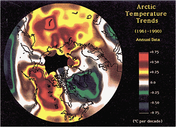
WALSH, FIGURE 4
Trends of temperature (°C per decade) computed using linear regression onto annual temperatures for 1961-1980. A Cressman analysis with a 400 km radius of influence has been applied to the computed trends. (From Chapman and Walsh, 1992; reprinted with permission of the American Meteorological Society.)
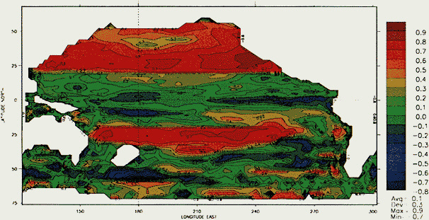
CAYAN ET AL., FIGURE 5a
Map of local correlations between ![]() and net heat-flux term on the right-hand side of Equation 4. Note that in the tropical strip ( ± 20° latitude), a Newtonian heat-flux parameterization is invoked and observed heat-flux anomalies are excluded.
and net heat-flux term on the right-hand side of Equation 4. Note that in the tropical strip ( ± 20° latitude), a Newtonian heat-flux parameterization is invoked and observed heat-flux anomalies are excluded.
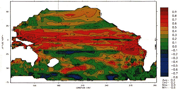
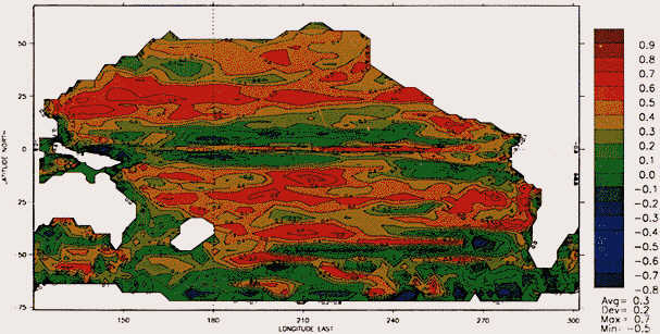
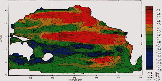
CAYAN ET AL., FIGURE 7
Map of local correlation coefficients between model and observed SST anomalies for all months, 1970-1988. Note that in the tropical strip (± 20° latitude), a Newtonian heat-flux parameterization is invoked and observed heat-flux anomalies are excluded.
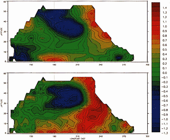
CAYAN ET AL., FIGURE 9
Difference fields of SST (°C) for the winters of 1976-77 through 1981-82 minus those of 1970-71 through 1975-76, for the model (top) and observations (bottom).
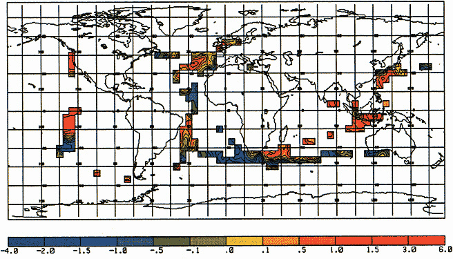
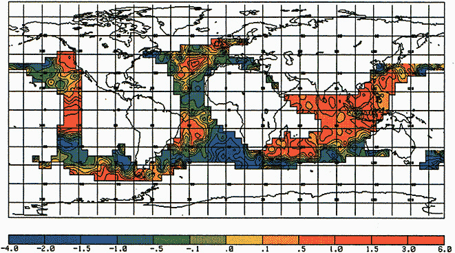
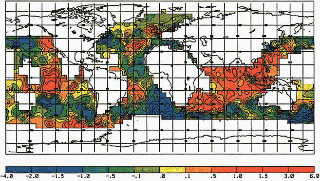
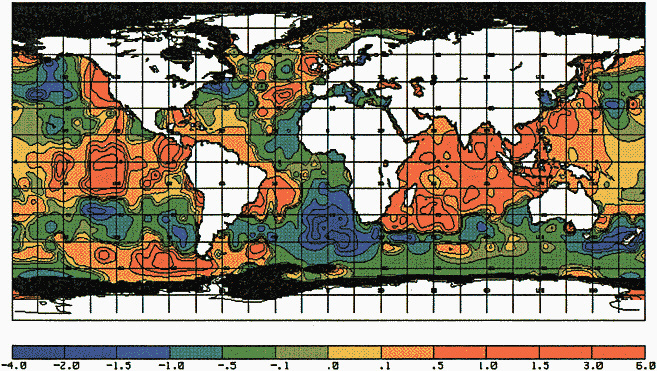
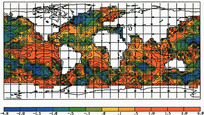
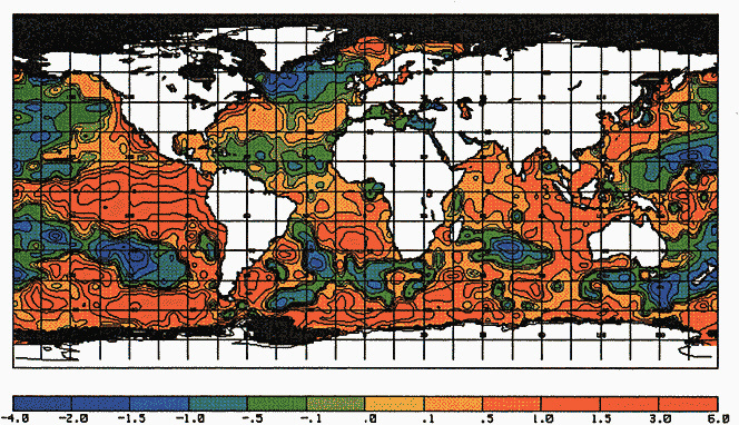
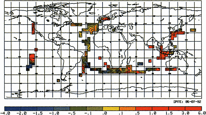
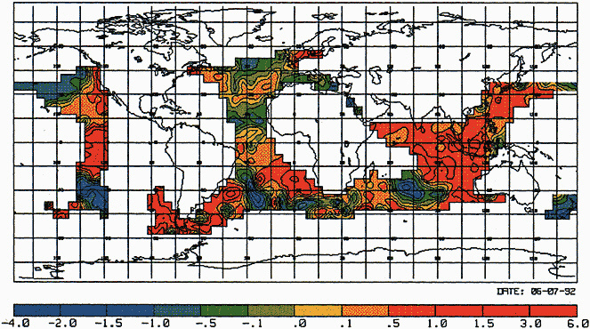
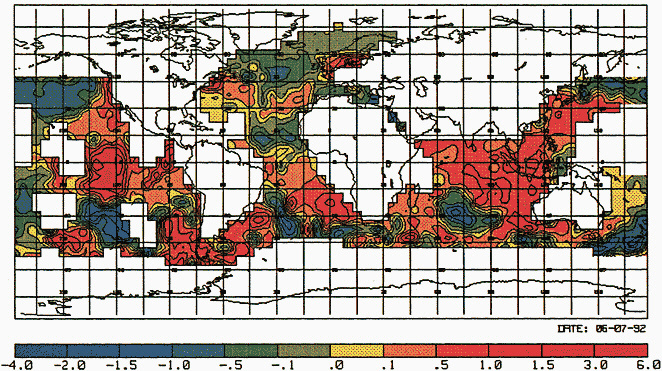
PARKER ET AL., FIGURE 4c
Enhanced MOHSST5 anomalies (°C), January 1983, with coverage of input data limited to that of 1877-1878.
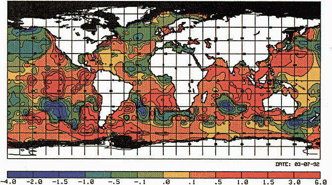
PARKER ET AL., FIGURE 4d
Globally complete SST anomalies (°C) and sea ice, January 1983, with coverage of input SST data limited to that of 1877-1878. Sea ice is shaded black.
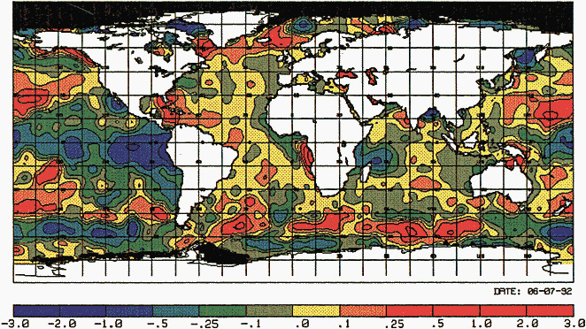
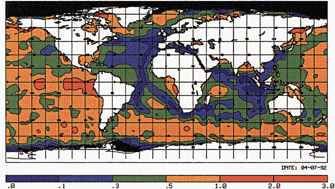
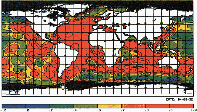
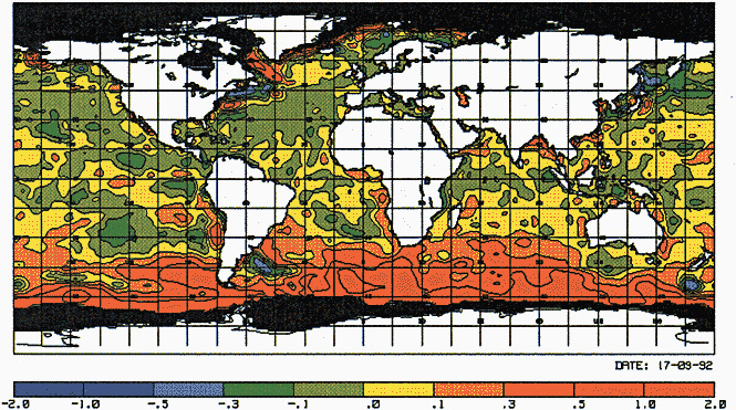
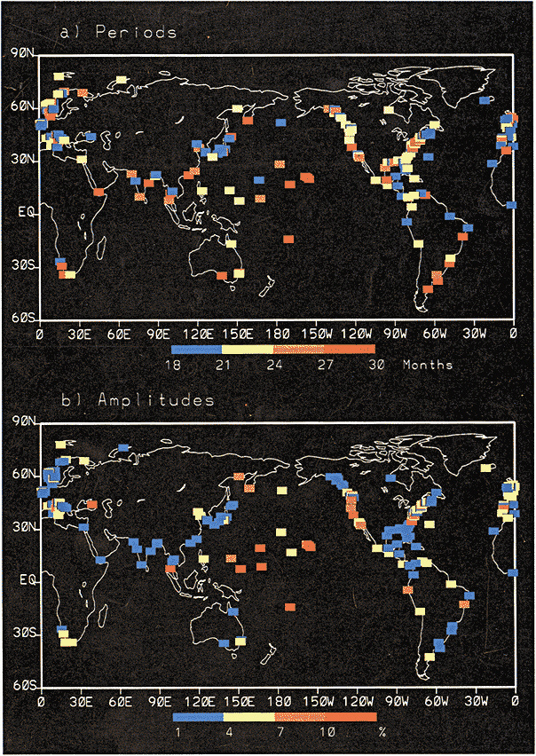
GHIL, COMMENTARY ON DOUGLAS, FIGURE 1
Distribution of stations that show an oscillatory feature with periods from 18 to 30 months. (a) distribution of period; (b) distribution of the amplitudes of the quasi-biennial oscillation, as a percentage of the total variance at each station (courtesy of Y. Sezginer-Unal).
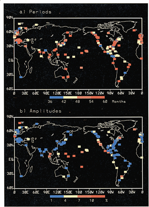
GHIL, COMMENTARY ON DOUGLAS, FIGURE 2
Distribution of the stations that show an oscillatory feature with periods from 36 months to 60 months. (a) distribution of the period; (b) distribution of the amplitudes of the low-frequency ENSO signal, as a percentage of the total variance at each station (courtesy of Y. Sezginer-Unal).
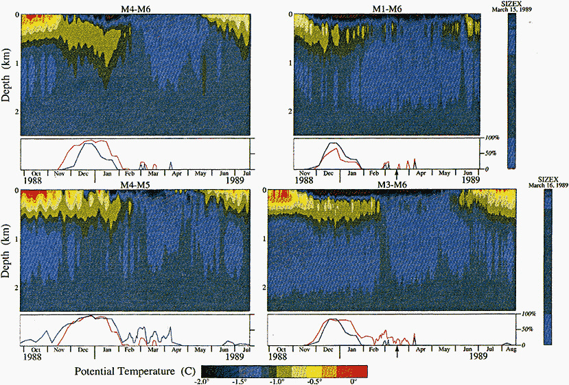
MUNK, DISCUSSION FOLLOWING LAZIER PAPER, FIGURE 1
Time series of range-averaged potential temperature profiles along four paths of the tomogra Total ice concentration in percent (from SSMM/I data) at the path endpoints are plotted below the images. Range-averaged profiles, computed from Seasonal Ice Zone E (SIZEX) data obtained on 15-16 March 1989 between moorings 1 and 6 and moorings 3 and 6 are given for comparison. (From SIZEX group, 1989; reprinted with permis Nauseu Remote Sensing Center.)
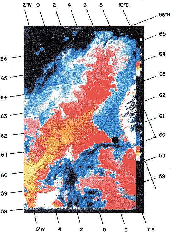
LEHMAN, FIGURE 8
Advanced VHR radiometer image of the eastern Norwegian Sea, showing the entry of warm Atlantic waters (warm colors) between the Faeroe and Shetland islands and the mixing of Atlantic waters into the North Sea. The site of Troll 3.1 is marked (![]() ). The dark, northeast-arching swath near the core site reflects cloud cover. (From Johannessen, 1986: reprinted with permission of Springer-Verlag.)
). The dark, northeast-arching swath near the core site reflects cloud cover. (From Johannessen, 1986: reprinted with permission of Springer-Verlag.)


